Bull. Sci. math.125, 6-7 (2001) 623–640

2001 Éditions scientifiques et médicales Elsevier SAS. All rights reserved

S0007-4497(01)01102-2/FLA

GROUND STATE ESTIMATIONS IN GAUGE THEORY

BY

ANA-BELA CRUZEIROa, PAUL MALLIAVIN b,SETSUO TANIGUCHI c

aDet. de Matematica I.S.T. and Grupo de Fisica-Matematica, Av. Prof. Gama Pinto 2,1649-003 Lisboa, Portugal

b10 rue St Louis en l’Ile, 75004 Paris, FrancecFaculty of Mathematics, Kyushu University, Fukuoka 812-8581, Japan

ABSTRACT. – The lowest eigenvalueλ(F) of a vector bundleF over a compactRiemannian manifoldM is estimated in terms of the curvature ofM and of theconnectionΓ onF . 2001 Éditions scientifiques et médicales Elsevier SAS

Introduction

Given a compact Riemannian manifoldM and an Euclidean vectorbundleF → M , we choose an Euclidean connectionΓ overF . Then theLaplace–Beltrami operator of M is lifted through the connectionΓinto an elliptic operator operating on the sections ofF . We shalldiscuss in this paper the problem of estimating the lowest eigenvalueλ(F ) in terms of the curvature ofM and ofΓ . The first part is devoted tothe majoration of the ground state under an assumption of Ricci positivityof the base manifoldM ; we shall get such a majoration in the caseof abelian gauge group; on the contrary a counter example using spinrepresentation will show that such majoration does not remain true in thecase of non abelian gauge group.

The second part will establish a universal minoration, which validseven if M is non-simply connected, and in non-abelian gauge theory.We shall develop this estimate at the level of frame bundle; but ourmethodology can be applied to the case where the gauge is an arbitraryprincipal bundle overM .

624 A.-B. CRUZEIRO ET AL. / Bull. Sci. math. 125 (2001) 623–640

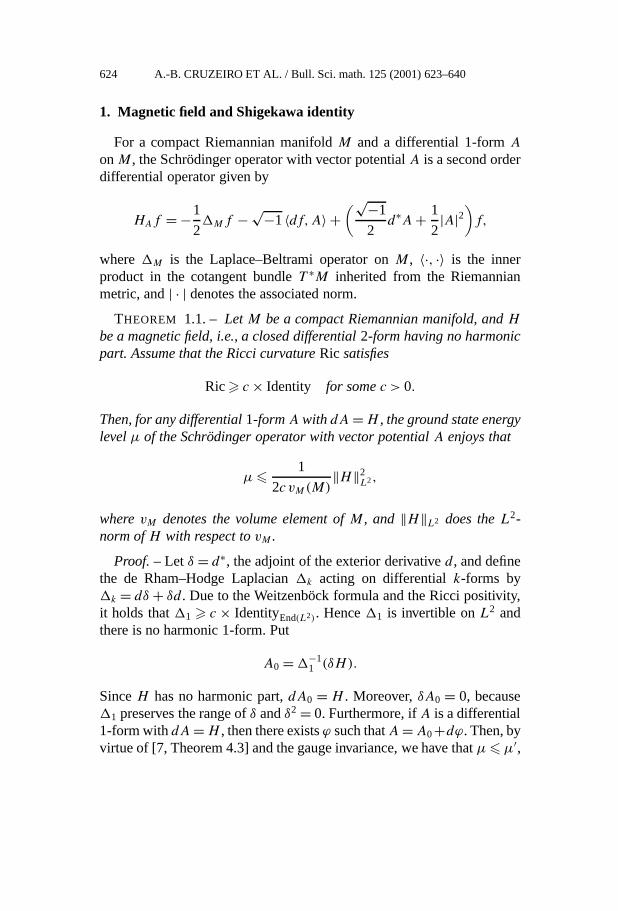
1. Magnetic field and Shigekawa identity

For a compact Riemannian manifoldM and a differential 1-formAonM , the Schrödinger operator with vector potentialA is a second orderdifferential operator given by

HAf = −1

2Mf − √−1〈df,A〉 +

(√−1

2d∗A + 1

2|A|2

)f,

whereM is the Laplace–Beltrami operator onM , 〈·, ·〉 is the innerproduct in the cotangent bundleT ∗M inherited from the Riemannianmetric, and| · | denotes the associated norm.

THEOREM 1.1. – Let M be a compact Riemannian manifold, andH

be a magnetic field, i.e., a closed differential2-form having no harmonicpart. Assume that the Ricci curvatureRic satisfies

Ric c × Identity for somec > 0.

Then, for any differential1-formA with dA = H , the ground state energylevelµ of the Schrödinger operator with vector potentialA enjoys that

µ 1

2c vM(M)‖H‖2

L2,

wherevM denotes the volume element ofM , and ‖H‖L2 does theL2-norm ofH with respect tovM .

Proof. –Let δ = d∗, the adjoint of the exterior derivatived, and definethe de Rham–Hodge Laplaciank acting on differentialk-forms byk = dδ + δd. Due to the Weitzenböck formula and the Ricci positivity,it holds that1 c × IdentityEnd(L2). Hence1 is invertible onL2 andthere is no harmonic 1-form. Put

A0 = −11 (δH).

SinceH has no harmonic part,dA0 = H . Moreover,δA0 = 0, because1 preserves the range ofδ andδ2 = 0. Furthermore, ifA is a differential1-form withdA = H , then there existsϕ such thatA = A0+dϕ. Then, byvirtue of [7, Theorem 4.3] and the gauge invariance, we have thatµ µ′,

A.-B. CRUZEIRO ET AL. / Bull. Sci. math. 125 (2001) 623–640 625

whereµ′ is the smallest eigenvalue of the operator120 + 1

2‖A0(·)‖2,‖A0(x)‖ being the norm ofA(x) in T ∗

x M . The eigenvalueµ′ correspondsto minimizing the Dirichlet form∫

M

‖dφ(x)‖2 + 1

2‖A0(x)‖2|φ(x)|2

vM(dx)

over φ ∈ C∞(M) with ‖φ‖L2 = 1. Hence, substituting a test functionφ ≡ 1/

√vM(M), we obtain

µ′ ‖A0‖2L2

2vM(M).(1.1)

Due to the Weitzenböck formula and the Ricci positivity, we obtain that

‖H‖2L2 = ‖dA0‖2

L2 =∫M

⟨A0(x),1A0(x)

⟩T ∗x M

vM(dx) c‖A0‖2L2.

Plugging this into (1.1) we obtain the desired estimation.Remark1.1. – Lévy’s formula implies that, onR2, the constant

magnetic fieldH = λdx ∧ dy of intensity λ ∈ R has the ground stateenergy level|λ|/2. By Theorem 1.1, in the case of compact manifoldwith positive Ricci curvature, we get an asymptotic behaviour of orderO(λ2) asλ → 0.

The Aharonov–Bohm effect appears in a solenoidal circuit, whichcomes out of the Ricci positivity.

2. Flat spin bundle with a positive ground state

Let Q be the skew field of quaternion numbers. It is generated bye, i, j , andk, e being the unit element, and the algebraic operations aregiven by

(te + xi + yj + zk) + (t ′e + x′i + y′j + z′k)= (t + t ′)e + (x + x′)i + (y + y′)j + (z + z′)k,

ij = k, jk = i, ki = j, i2 = j2 = k2 = −e.

626 A.-B. CRUZEIRO ET AL. / Bull. Sci. math. 125 (2001) 623–640

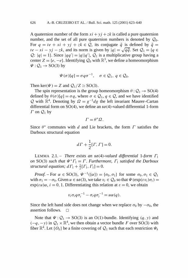
A quaternion number of the formxi +yj + zk is called a pure quaternionnumber, and the set of all pure quaternion numbers is denoted byQ0.For q = te + xi + yj + zk ∈ Q, its conjugateq is defined byq =te − xi − yj − zk, and its norm is given by|q| = √

qq. SetQ1 = q ∈Q: |q| = 1. Since|qq ′| = |q||q ′|, Q1 is a multiplicative group having acenterZ = e,−e. IdentifyingQ0 with R

3, we define a homeomorphismΨ :Q1 → SO(3) by

Ψ (σ )[q] = σqσ−1, σ ∈ Q1, q ∈ Q0.

Then ker(Ψ ) = Z andQ1/Z SO(3).The spin representation is the group homeomorphismθ :Q1 → SO(4)

defined byθ(σ )[q] = σq, whereσ ∈ Q1, q ∈ Q, and we have identifiedQ with R

4. Denoting byΩ = g−1dg the left invariant Maurer–Cartandifferential form on SO(4), we define anso(4)-valued differential 1-formΓ onQ1 by

Γ = θ∗Ω.

Sinceθ∗ commutes withd and Lie brackets, the formΓ satisfies theDarboux structural equation

dΓ + 1

2[Γ,Γ ] = 0.

LEMMA 2.1. – There exists anso(4)-valued differential1-form Γ1

on SO(3) such thatΨ ∗Γ1 = Γ . Furthermore,Γ1 satisfied the Darbouxstructural equation;dΓ1 + 1

2[Γ1,Γ1] = 0.

Proof. –For α ∈ SO(3), Ψ −1(α) = σ0, σ1 for someσ0, σ1 ∈ Q1

with σ1 = −σ0. Givenu ∈ so(3), we takevi ∈ Q0 so thatΨ (exp(εvi)σi) =exp(εu)α, i = 0,1. Differentiating this relation atε = 0, we obtain

viσiqσ−1i − σiqσ

−1i = uα(q).

Since the left hand side does not change when we replaceσ0 by −σ0, theassertion follows.

Note thatΨ :Q1 → SO(3) is an O(1)-bundle. Identifying(q, y) and(−q,−y) in Q1 × R

4, we then obtain a vector bundleF over SO(3) withfiberR

4. Let Ok be a finite covering ofQ1 such that each restrictionΨk

A.-B. CRUZEIRO ET AL. / Bull. Sci. math. 125 (2001) 623–640 627

of Ψ to Ok is injective. PutΩk = Ψ (Ok) and consider the trivial vectorbundleFk = Ok × R

4 overOk . Then, via the reciprocal image(Ψ −1k )∗Fk ,

we get a coherent family of vector bundles overΩk , which determinesthe vector bundleF over SO(3) as above.

Let E = Q1 × R4 be the trivial bundle overQ1. The space of smooth

sectionsΓ ∞(E) of the vector bundleE overQ1 can be identified withC∞(Q1;R

4). Under this identification, the covariant derivative∇(1) isdefined by∇(1)s = ds + Γ · s, s ∈ C∞(Q1;R

4). By the definition of thevector bundleF over SO(3), denoting byΓ ∞(F ) the smooth sections ofF , we have the identification

Γ ∞(F ) = s ∈ C∞(Q1;R

4): s(−q) = −s(q), q ∈ Q1.(2.1)

By Lemma 2.1, we see that the covariant derivative∇(1) admits arestriction toΓ ∞(F ), say∇F , and that the curvature associated with∇F

vanishes.Under the identification betweenQ andR

4, Q1 is identified with the3-sphereS3. Hence it is equipped with the Riemannian metric inheritedfrom the standard flat metric ofR4. ThenQ1 is a compact manifold withpositive Ricci curvature. The Riemannian metric onQ1 induces that onSO(3). Consider the Brownian loopmω(t) on SO(3) starting and endingat the identity at time 0 andT , respectively. It is lifted to the processqωonQ1 with qω(0) = e andqω(T ) ∈ Z = ±e. Let νT be the law ofqω(T )

onZ.

LEMMA 2.2. – There existsC,c > 0, which is independent ofT , suchthat

0< νT (e) − νT (−e) C exp(−cT ).(2.2)

Proof. –Let p(t, q, q ′) be the heat kernel associated with the Laplace–Beltrami operator onQ1. Then we have

νT (e) = p(T , e, e)

p(T , e, e) + p(T , e,−e),

νT (−e) = p(T , e,−e)

p(T , e, e) + p(T , e,−e).

(2.3)

Due to the Ricci positivity ofQ1, there existsC,c > 0 such that

628 A.-B. CRUZEIRO ET AL. / Bull. Sci. math. 125 (2001) 623–640

supq∈Q1

∣∣∣∣∫Q1

f (r)p(T , q, v)vQ1(dv) − 1

vQ1(Q1)

∫Q1

f (v)vQ1(dv)

∣∣∣∣(2.4)

C‖df ‖∞e−cT

for anyT > 0 andf ∈ C∞(Q1), wherevQ1 stands for the volume elementof Q1 and ‖ · ‖∞ does the uniform norm onQ1. For example, see [8,Theorem 6.22]. Substitutingp(1, ·, e) − p(1, ·,−e) andp(1, ·, e) for f

in (2.4), we obtain that∣∣p(T +1, e, e)−p(T +1, e,−e)∣∣ C

∥∥d[p(1, ·, e)−p(1, ·,−e)]∥∥∞e−cT

and

supq∈Q1

∣∣∣∣p(T + 1, e, q) − 1

vQ1(Q1)

∣∣∣∣ C∥∥d[p(1, ·, e)]∥∥∞e−cT(2.5)

for anyT > 0. In conjunction with (2.3), these imply the upper estimationin (2.2).

To see the lower estimation in (2.2), letq ′ω(t) be the Brownian motion

onQ1 starting ate andmω(t) = Ψ (q ′ω(t)). Denoting byP the underlying

probability measure, we obtain

νT (e) = P(q ′(T ) = e | m′(T ) = Id

),

νT (−e) = P(q ′(T ) = −e | m′(T ) = Id

).

SetΛ = inft 0: q ′(t) ∈ Q0 ∩ Q1. By virtue of the Markov propertyand the symmetry of the Brownian motion onQ1, we have

P(q ′(T ) = e,Λ< T | m′(T ) = e

)= P(q ′(T ) = −e,Λ< T | m′(T ) = e

).

SinceP(q ′(T ) = −e,Λ T | m′(T ) = Id) = 0, we arrive at

νT (e) − νT (−e) = P(q ′(T ) = e,Λ T | m′(T ) = Id

)> 0.

Thus the lower estimation in (2.2) has been verified.THEOREM 2.1. – The bundleF with the covariant derivative∇F as

described above has a null curvature, and the base manifoldSO(3) has astrictly positive Ricci curvature. Moreover, the ground stateλ(F ) of thecovariant Laplacian associated with∇F satisfiesλ(F ) c, wherec > 0is the constant which appeared in Lemma2.2.

A.-B. CRUZEIRO ET AL. / Bull. Sci. math. 125 (2001) 623–640 629

Proof. –Let k(t,m,m′) be the heat kernel for the covariant Laplacianassociated with∇F . As in the previous lemma, we denote byq ′

ω(t) theBrownian motion onQ1 and setq ′

ω(t, q) = q ′ω(t)q for q ∈ Q1. Define

eω(t, q) ∈ SO(4) by

deω(t, q) = −Γ(q ′ω(t, q)

)eω(t, q) dq ′

ω(t, q), eω(0, q) = Id.

Then, by the identification (2.1), forq, q ′ with Ψ (q) = m andΨ (q ′) =m′, we have

k(t,m,m′) = E[eω(t, q)

−1δq ′(q ′ω(t, q)

)− δ−q ′(q ′ω(t, q)

)],

whereδq(· · ·) stands for Watanabe’s pullback of the Dirac function viaq ′ω(t, q). This yield that

k(t,m,m) = E[eω(t, q)

−1δe(q ′ω(t)

)− δ−e

(q ′ω(t)

)].

Thus we obtain⟨ξ, k(t,m,m)ξ

⟩= |ξ |2p(t, e, e) + p(t, e,−e)

νT (e) − νT (−e)for anyξ ∈ R

4, which, in conjunction with Lemma 2.2 and (2.5), impliesthe desired estimation ofλ(F ). 3. Anticipative tangent process and transversal analytic

hypoellipticity

3.1. Calculus of variation on O(M)

Let X be the Wiener space of thed-dimensional Brownian motion andµ be the Wiener measure on it. An anticipating tangential process is aprocessζ onX of the form

dζ α(τ) = aαβ (τ) dx

β(τ) + cα(τ) dτ,

where aαβ = −aβ

α , ααβ(0) = 0, cα(0) = 0, E[∫ 1

0 |c|2 dτ ] < ∞, and aαβ

may not be adapted, and hence the integral should be understood asa Skorohod stochastic integral (the standard summation convention hasbeen used).

630 A.-B. CRUZEIRO ET AL. / Bull. Sci. math. 125 (2001) 623–640

Let O(M) be the the orthonormal frame bundle overM . ThenO(M)

admits the canonical parallelization; i.e., there exists a differential 1-formΘ = (Θ, Θ) with values inRd ×so(d) such that, for everyr ∈ O(M), Θr

is an isomorphism ofTrO(M) onto Rd × so(d). Using this parallelism,

we can define, the horizontal Brownian motionrx(τ, r0) on O(M)

starting atr0, which defines a horizontal flowUxτ←0(r0) := rx(τ, r0).

Denoting byR andΩ the Ricci curvature and the curvature tensor ofthe Riemannian manifoldM , we link two tangent processesζ andζ ′ bythe relation

dζ = dζ ′ + 1

2R(ζ ′) dτ + ρ dx(τ),(3.1.1)

dρ = Ω(dx, ζ ′),(3.1.2)

where R and Ω are both scalarized with the framer ∈ O(M), andevaluated atr(τ, r0).

To handle the stochastic calculus of variation for anticipating tangentprocesses, we generalize the result for adapted tangent processes obtainedin [1].

PROPOSITION 3.1.1. – Let ζ, ζ ′ be as above. Then, an infinitesimalvariation x !→ x + εζ of x ∈ X induces a variation of the horizontalflow Ux , which is represented in terms of the canonical parallelismof O(M) as follows: (

ζ ′(∗), ρ(∗)).(3.1.3)

Proof. –It is sufficient to treat the casedξ ′α = φaα,β dx

β with a adaptedand φ a smooth functional, the stochastic integral being a Skorohodintegral. We denotedξ ′

α = φaα,β dxβ , then

ξ ′α(τ) = φ

τ∫0

aα,β dxβ − h′

α(τ)

with h′α(τ) = ∫ τ

0 (Dη,βφ)aα,β dη. For a smooth functionalF on the pathspace,

(Dξ ′F) I = (φ I )Dξ (F I ) − Dh(F I ),

where

dξ = dξ ′ − ρ dx, dρ = Ω(ξ ′,dx)

A.-B. CRUZEIRO ET AL. / Bull. Sci. math. 125 (2001) 623–640 631

and

dh = dh′ − ρ dx, dρ = Ω(h′,dx).We have(φ I )ξα(τ ) = ξ ′

α(τ) + h′α(τ) − ζα(τ), where

ζα(τ) =τ∫

0

[ η∫0

Ωγ,αλ,δ

(φξ ′)λ dxδ

] dxγ

and

(Dξ ′F) I = (Dξ + D∫ .

0ρdx − Dζ)(F I ) = Dξ(F I ),

dξ = dξ − ρ∗ dx, dρ∗α = −ρα dx +

( τ∫0

Ω.,αλ,δ

(φξ ′)λ dxδ

) dx.

Sincedρ∗α = ∫ τ

0 (Ω.,αλ,δ(φξ

′ − h′)λ dxδ) = ∫ τ

0 Ωα(ξ ′,dx), the result isproved.

COROLLARY 3.1.1. – Define

Φβ(x, τ) =τ∫

0

Ωα,β dxα,

whereΩ is again the scalarization of the curvature tensor atrx(τ, r0),which is thought of as a mapping ofR

d × Rd → so(d), andΩα,β is the

evaluation of this map at(eα, eβ), eα being the standard coordinateof R

d . If ζ ′(t) = 0, then

ρ(t) = −t∫

0

Φβ(τ) dζ ′β(τ).

Proof. –The assertion follows by applying an integration by parts inthe variableτ . 3.2. A variance analysis

Denote byεγ,δ;1 γ < δ d the canonical basis ofso(d), andsimply we writeθ for (γ, δ). The functionalΦβ defined in Corollary 3.1.1

632 A.-B. CRUZEIRO ET AL. / Bull. Sci. math. 125 (2001) 623–640

takes values inso(d) and is expressed asΦβ = ∑θ Φ

βθ εθ . Fixing t ∈

(0,1), for a functionΨ on [0,1], we set #Ψ = 1t

∫ t

0 Ψ and Ψ = Ψ −#Ψ . Throughout the remainder of this section, we do not indicate thedependence ont explicitly to keep the notation simple, while mostquantities appearing later depend ont . Define acovariance matrixby

σ θ ′θ =∑

β

t∫0

Φβθ (τ )Φ

βθ ′(τ ) dτ.(3.2.1)

PROPOSITION 3.2.1. – Let A ∈ so(d). If σ defined in (3.2.1) isinvertible, thencβ defined by

cβ(τ) =∑θ

aθ Φβθ (τ ), whereaθ =∑

θ ′

[σ−1]θ ′

θAθ ′,(3.2.2)

satisfy

∑β

t∫0

Φβθ (τ )cβ(τ) dτ = Aθ .(3.2.3)

Proof. –Substituting (3.2.2) into the left hand side of (3.2.3), we obtain∑θ

σ θθ ′aθ = Aθ ′,

which implies the assertion.Using the abovecβ ’s, we define a tangent processζ ′ by ζ ′

β(τ) =∫ τ

0 cβ(s) ds. Then ζ ′(t) = 0, and, by Corollary 3.1.1,ρ(t) = A. ByLemma 3.1.1, the corresponding infinitesimal variation is due toζ

defined by (3.1.1) with theseζ ′ andρ.The processΦβ itself is adapted, and the non-adaptedness comes

from #Φβ andσ−1.

3.3. Stochastic calculus of variation for small time

We would like to estimate the behavior ofσ−1 ast → 0. We first noticethat

E[σ θ ′θ

]= t2

2Γ θ ′

θ (r0) + o(t2) (t → 0),(3.3.1)

A.-B. CRUZEIRO ET AL. / Bull. Sci. math. 125 (2001) 623–640 633

whereΓ θ ′θ (r0) =∑

α,β Ωα,β;θ (r0)Ωα,β;θ ′(r0), but the identity (3.3.1) givesno a.s. estimation ofσ−1. To obtain an estimation ofσ−1, we needan assumption on the curvature tensor. To state this, note that, atevery pointr ∈ O(M), the curvature tensorΩ determines a symmetricendomorphism ofΛ2(Rd), the space of differential 2-forms onRd . Toemphasize that this endomorphism is considered, we write(Ω) or (Ω)rwith parentheses. Under the invertibility assumption of(Ω), we obtainthe estimation ofσ−1.

LEMMA 3.3.1. – Suppose that(Ω)r is invertible for everyr ∈ O(M).Then, for everyp > 1, there exist constantsCp(Ω) > 0 such that

E[‖σ−1‖p

] Cp(Ω)t−2p for any t ∈ (0,1].(3.3.2)

Proof. –Let rt (τ, x) be the horizontal Brownian motion onO(M) timechanged byt ; drt = √

tLα(rt ) dxα , whereLα is the system of the

canonical horizontal vector fields. Set

Ψβθ (τ) =

τ∫0

Ωα,β;θ(rt (s)

) dxα(s).

Then, by the time change argument, we obtain

σ θ ′θ = t2

∑β

1∫0

Ψβθ (τ )Ψ

β

θ ′ (τ ) dτ.

Put

σ θ ′θ =∑

β

1∫0

Ψβθ (τ )Ψ

β

θ ′ (τ ) dτ.

Since(Ω) is invertible, we have

infr∈O(M),A∈Λ2(Rd);‖A‖=1

∥∥(Ω)r [A]∥∥> 0.

634 A.-B. CRUZEIRO ET AL. / Bull. Sci. math. 125 (2001) 623–640

Hence there are a positive numberε > 0, an open coveringUiNi=1of O(M), and indices 1 β1, . . . , βN d such that

∑α

∣∣∣∣∑θ

Ωαβi ;θ(r)Aθ

∣∣∣∣2 ε

for any r ∈ Ui, A ∈ Λ2(Rd) with ‖A‖ = 1, andi = 1, . . . ,N . Then, inrepetition of the standard argument to show the nondegeneracy of theMalliavin covariance for the solution to an SDE with elliptic diffusioncoefficients (cf. [9]), we obtain

supt∈(0,1]

E[∥∥σ−1∥∥p]< ∞ for anyp > 1.

Thus the assertion has been shown.3.4. Approximate stochastic calculus of variations

We denote byΩ0 the curvature tensor frozen at the pointr0, andapproximateΦβ(x, τ) by ∑

α

Ω0α,βx

α(τ).

Introduce a Gaussian process

xα(τ ) = xα(τ) − 1[0,t )(τ )t∫

0

xα(s)ds

t.(3.4.1)

ThenΦβ is approximated by∑

α Ω0α,β xα(τ ), and the covariance matrixσ

is done by

σ0 = ∑α,α′,β

Ω0α,βΩ

0α′,βγα,α′(t),(3.4.2)

where

γα,α′(t) =t∫

0

xα(τ )xα′(τ ) dτ.

A.-B. CRUZEIRO ET AL. / Bull. Sci. math. 125 (2001) 623–640 635

LEMMA 3.4.1. – The symmetric matrixt−2γ (t) is a.s. positive defi-nite and has a law which is equal to the law ofγ (1). Furthermore, thereexistsc > 0, which can be explicitly computed, such that

µ(∥∥γ (t)−1∥∥>Mt−2) exp(−cM).

Proof. –The assertion can be found in [5] and [4].Thecβ in (3.2.2) are now approximated by

c0β =∑

α,θ

a0αΩ

0α,β;θ xα, wherea0

θ =∑θ ′

[σ−1

0

]θ ′θAθ ′ .

3.5. Estimating the divergence of a variation on the Wiener space

Using the above approximation method, we can estimate the diver-genceδ(ζ ) of ζ given in (3.1.1) withζ ′ andρ as described at the end ofthe Section 3.2. Settingλ(t) = √

γ (t), we have

σ0 = (Ω)r0 (λ ⊗ 1)

(Ω)r0 (λ ⊗ 1)

∗.(3.5.1)

THEOREM 3.5.1. – The divergenceδ(ζ ) satisfies

limt→0

tE[|δ(ζ )|] cd

∥∥(Ω)−1∥∥‖A‖,(3.5.2)

wherecd is a universal positive constant depending only on the dimen-siond, and can be computed.

For the proof, we prepare a lemma;

LEMMA 3.5.1. – Let xt denote the Brownian motion on[0, t] and(u(xt ))(η) = 1√

txt (tη) the isometry between the corresponding Wiener

spaces. Ifφ is a differentiable functional ofx1 thenF t(xt ) = φ(x) isdifferentiable and the following rescaling property holds:

DτFt(xt)= 1√

tDτ

tφ(x1).

In particular, it holds that

t E(DZt

0F t(xt))= E

(DZ1

0φ(x1)).

636 A.-B. CRUZEIRO ET AL. / Bull. Sci. math. 125 (2001) 623–640

Proof. –We shall prove the lemma for cylindrical smooth functionalsφ, the result being obtained by closure.

If φ(x1) = φ(x1(τ1), . . . , x1(τm)),

DtτF

t(xt)=∑

k

1τ<tτk ∂kφ

(xt (tτ1)√

t, . . . ,

xt (tτm)√t

)

=∑k

1τt <τk

1√t∂φ(x1(τ1), . . . , x

1(τm))

= Dτt

1√tφ(x1).

Since the matrixσ t0 = Ωα,βΩα′,β

∫ t

0 xtα(η)x

tα′(η) dη rescales asσ t

0 = t2σ 10 ,

we have

E(DZt

0F t(xt))

= E

[ t∫0

DtτF

t(xt)[σ t

0

]−1xt (τ ) dτ

]

= E

[ t∫0

1√tDτ

tφt−2[σ 1

0

]−1

(√tx1(τ

t

)− 1

t

t∫0

√tx

(s

t

)ds

)dτ

]

= E

[ 1∫0

Dλφt−2[σ 1

0

]−1x1(λ) t dλ

].

Proof of Theorem 3.5.1. –We shall estimate theL2 norms of thedivergence of the vector fields by using the equality

E[|δZ|2]= E

[∫|Z|2

]+ E

[∫ ∫DτZ(η).DηZ(τ)

].

Working with the curvature tensor frozen atr0 and at timet = 1 wehave the following estimate for theL2 norm of the correspondingapproximating vector fieldζ0:

E

[ 1∫0

∑β

∣∣[σ−10

]θ ′θAθ ′Φβ

θ (η)∣∣2 dη]

A.-B. CRUZEIRO ET AL. / Bull. Sci. math. 125 (2001) 623–640 637

= E

[ 1∫0

∑β

[σ−1

0

]θ ′θAθ ′Φβ

θ (η)[σ−1

0

]θ ′1θ1Aθ ′

1Φ

βθ1(η) dη

]

= E([σ−1

0

]θ ′θAθ ′[σ−1

0

]θ ′1θ1

[σ0]θ1θ Aθ ′

1

)= E

(⟨[σ−1

0

]A,A

⟩) E

∥∥σ−10

∥∥‖A‖2.

We now compute the derivatives ofσ and ofΦ; we have

Dτ,αΦβθ (η) =Dτ,α

∑α′

Ωθα′,β

(xα′(η) −

1∫0

xα′

)

=Ωα,βθ(1τ<η − (1− τ)

)and

[Dτ,ασ0]θ ′θ =

[Dτ,α

( ∑γ,γ ′,δ

Ωθγ,δΩ

θ ′γ ′,δ

1∫0

xγ (η)xγ ′(η) dη

)]

=∑γ,δ

(Ωθ

γ,δΩθ ′α,δ + Ωθ

α,δΩθ ′γ,δ

) 1∫0

xγ (η)(1τ<η − (1− τ)

)dη.

Therefore

E

[ 1∫0

1∫0

∑α,β

|Dτ,αcβ(η)|2 dτ dη

]

2E

[ 1∫0

1∫0

∑α,β

∣∣[σ−10

]θ ′θAθ ′Ωθ

α,β

(1τ<η − (1− τ)

)∣∣2dτ dη

]

+ 2E

[ 1∫0

1∫0

∑α,β

∣∣([σ−10

]Dτ,ασ0

[σ−1

0

])θ ′θAθ ′Φβ

θ (η)∣∣2dτ dη

]

2E[∥∥σ−1

0

∥∥2‖A‖2‖Ω‖2]+ 2cE[∥∥σ−1

0

∥∥4‖A‖2‖Ω‖4].The final result follows from (3.5.1), Lemma 3.5.1, which shows that

tδ(ζ t0) = δ(ζ 1

0 ), where the superscriptt and 1 is used to indicate thedependence ont explicitly, and the convergence

limt→0

tE[∥∥δ(ζ t − ζ t

0

)∥∥] limt→0

t∥∥ζ t − ζ t

0

∥∥W2

1= 0.

638 A.-B. CRUZEIRO ET AL. / Bull. Sci. math. 125 (2001) 623–640

The last convergence is a consequence of a.e. convergence of theintegrands and anLp, p > 1, uniform boundedness int of them. Namely,from the estimates of the expectations of stochastic integrals, we have

t2E∥∥ζ t∥∥2 t2

E

t∫0

∥∥σ−1AΦ(η)∥∥2

t2‖A‖2(E∥∥σ−1∥∥4)1/2

(E

[ t∫0

∥∥Φ(η)∥∥2

]2)1/2

C4(Ω)1/2‖A‖2,

where we have dropped the indices for the sake of simplicity.Concerning the first order term, we have

t2E∥∥Dζ t

∥∥2 2t2E

( t∫0

t∫0

∥∥σ−1ADτΦ(η)∥∥2

dη

)1/2

+ 2t2E

( t∫0

t∫0

∥∥σ−1∥∥2‖Dτσ‖2∥∥σ−1∥∥2‖A‖2∥∥Φ∥∥2dη

)1/2

.

This term is much more messy but can be treated in an analogous way,as long as we can rely on the Lemma 3.3.1. Indeed, by the expressionfor the derivation of stochastic integrals, the matricesDτσ has the samedependence ont asσ itself, which makes the estimation of all terms verymuch alike. 3.6. Transversal analyticity

Let (Ω)r be the endomorphism ofΛ2(Rd) defied by the curvaturetensorΩ at r ∈ O(M), and set

cΩ = supr∈O(M)

∥∥[(Ω)r ]−1∥∥ ∞.

Suppose thatcΩ < ∞, i.e. (Ω)r is invertible at everyr ∈ O(M). LetLα be the system of the canonical horizontal vector fields onO(M).Then [Lα,Lβ] is vertical andΩα,β;θ = −Θθ ([Lα,Lβ]), Θ being thesecond component of the canonical parallelismΘ on O(M). Thus the

A.-B. CRUZEIRO ET AL. / Bull. Sci. math. 125 (2001) 623–640 639

invertibility of (Ω)r implies thatLα satisfies the Hörmander condition,and hence there exists the heat kernel corresponding toO(M)/2, whereO(M) =∑

α(Lα)2 is the horizontal Laplacian onO(M).

THEOREM 3.6.1. – Let πt(r0, r) be the heat kernel associated withO(M)/2, the half of the holizontal Laplacian onO(M). Then, for anyr0 ∈ O(M) andA ∈ so(d), it holds that

lim supt→0

t

‖A‖∫

O(M)

|∂Aπt(r0, r)|vO(M)(dr) cdcΩ,(3.6.1)

where∂A stands for the vertical differentiation in the directionA, vO(M)

is the volume element ofO(M), andcd is a universal constant dependingonly on the dimensiond of M . Furthermore, the functionO(d) % g !→πt(r0, gr) possesses a holomorphic extension to the open set

Ot = γ ∈ SGL(Cd): γ = g exph, g ∈ SO(d), ‖h‖ < t/(ecdcΩ)

.

Proof. –Applying an integration by parts on the Wiener space andTheorem 3.5.1, we obtain (3.6.1). To show that the second assertionfollows from (3.6.1), see [6]. 4. Asymptotic estimate of ground state

Following the method of [6], the transversal analyticity obtained inTheorem 3.6.1, implies asymptotic bounds for the ground states of fiberbundles associated with representations of the orthogonal groups withlarge dominant weights.

REFERENCES

[1] Cruzeiro A.B., Malliavin P., Renormalized differential geometry on path space:structural equation, curvature, J. Funct. Anal. 139 (1996) 119–181.

[2] Cruzeiro A.B., Malliavin P., Nonperturbative construction of invariant measurethrough confinement by curvature, J. Math. Pures Appl. 77 (1998) 527–537.

[3] Cruzeiro A.B., Malliavin P., A class of anticipative tangent processes on the Wienerspace, C. R. Acad. Sci. Paris 333 (2001) 353–358.

[4] Kusuoka S., Stroock D.W., Applications of the Malliavin calculus, II, J. Fac. ScienceUniv. Tokyo 32 (1985) 1–76.

640 A.-B. CRUZEIRO ET AL. / Bull. Sci. math. 125 (2001) 623–640

[5] Malliavin P.,Ck hypoellipticity with degeneracy, in: Friedman A., Pinsky M. (Eds.),Stochastic Analysis, Academic Press, 1978, pp. 327–340.

[6] Malliavin P., Analyticité transverse d’opérateurs hypoelliptiquesC3 sur des fibrésprincipaux. Spectre équivariant et courbure, C. R. Acad. Sci. Paris 301 (1985) 767–770.

[7] Shigekawa I., Eigenvalue problems for the Schrödinger operators with the magneticfield on a compact Riemannian manifold, J. Funct. Anal. 75 (1987) 92–127.

[8] Stroock D.W., An Introduction to the Analysis of Paths on a Riemannian Manifold,AMS, 2000.

[9] Watanabe S., Stochastic Differential Equations and Malliavin Calculus, Tata Inst.Lect. Notes, Springer-Verlag, 1984.