arX

iv:h

ep-t

h/04

0707

6v2

19

Oct

200

9

N = (1, 1) super Yang–Mills theory in 1+1dimensions at finite temperature

John R. Hiller

Department of Physics

University of Minnesota Duluth

Duluth MN 55812

Yiannis Proestos, Stephen Pinsky, and Nathan Salwen

Department of Physics

Ohio State University

Columbus OH 43210

Abstract

We present a formulation of N = (1, 1) super Yang–Mills theory in1+1 dimensions at finite temperature. The partition function is con-structed by finding a numerical approximation to the entire spectrum.We solve numerically for the spectrum using Supersymmetric DiscreteLight-Cone Quantization (SDLCQ) in the large-Nc approximation andcalculate the density of states. We find that the density of states growsexponentially and the theory has a Hagedorn temperature, which weextract. We find that the Hagedorn temperature at infinite resolutionis slightly less than one in units of

√

g2Nc/π. We use the densityof states to also calculate a standard set of thermodynamic functionsbelow the Hagedorn temperature. In this temperature range, we findthat the thermodynamics is dominated by the massless states of thetheory.

1 Introduction

In N = 4 super Yang–Mills theory at largeNc, there is a known mismatch be-tween weak and strong coupling by a factor of 3/4 in the free energy [1]. Theweak-coupling result is calculable in perturbation theory; the strong-couplingresult comes from black-hole thermodynamics. It would be interesting to beable to directly solve this theory at all couplings and see the transition be-tween the weak-coupling and strong-coupling limits [2]. Analytically this isgenerally not possible, although there have been a number of early discussionsof methods for finite-temperature solutions to supersymmetric quantum fieldtheory [3]. We will instead consider a numerical method based on Supersym-metric Discrete Light-Cone Quantization (SDLCQ) [4, 5], which preservesthe supersymmetry exactly. Currently this is the only method available fornumerically solving strongly coupled super Yang–Mills theories. Conven-tional lattice methods have difficulty with supersymmetric theories becauseof the asymmetric way that fermions and bosons are treated, and progress [6]in supersymmetric lattice gauge theory has been relatively slow.

Given that SDLCQ makes use of light-cone coordinates, with x+ = (x0 +x3)/

√2 the time variable and p− = (p0 − p3)/

√2 the energy, we must take

some care in defining thermodynamic quantities. The seemingly naturalchoice [7] of e−βLC

p− as the partition function has been shown by Alves andDas [8] to lead to singular results for well known quantities that are finitein the equal-time approach. They argue that using e−βLC

p− for the partitionfunction implies that the physical system is in contact with a heat bath thathas been boosted to the light-cone frame and that this is not equivalent tothe physics of a system in contact with a heat bath at rest.

A more direct way to see this is that, since the light-cone momentump+ = (p0 + p3)/

√2 is conserved, the partition function must include it in

the form Z = e−βLC(p−+µp+), with µ its chemical potential. The interpreta-

tion of the chemical potential is that of a rotation of the quantization axis.Thus µ = 1 corresponds to quantization in an equal-time frame, where theheat bath is at rest and the inverse temperature β =

√2β

LC, and µ 6= 1

corresponds to quantization in a boosted frame where the heat bath is notat rest. Thus µ corresponds to a continuous rotation of the axis of quanti-zation, and µ = 0 would correspond to rotation all the way to the light-coneframe. A rotation from an equal-time frame to the light-cone frame is not aLorentz transformation. It is known that such a transformation can give riseto singular results for physical quantities. This appears to be consistent with

1

the results found in [8]. A number of related issues have been extensivelydiscussed by Weldon [9]. The method has also recently been applied to theNambu–Jona-Lasinio model [10].

These difficulties are avoided if we compute the equal-time partition func-tion Z = e−βp

0

, as was proposed much earlier by Elser and Kalloniatis [11].The computation may, of course, still use light-cone coordinates. Elser andKalloniatis did this with ordinary DLCQ [12, 13] as the numerical approxi-mation to (1+1)-dimensional quantum electrodynamics. Here we will followa similar approach using SDLCQ to calculate the spectrum of N = (1, 1)super Yang–Mills theory in 1+1 dimensions [14]. Though this calculationis done in 1+1 dimensions, it is known that SDLCQ can be extended in astraightforward manner to higher dimensions [15, 16, 17].

We have discussed the SDLCQ numerical method in a number of otherplaces, and we will not present a detailed discussion of the method here; for areview, see [5]. For those familiar with DLCQ [12, 13], it suffices to say thatSDLCQ is similar; both have discrete momenta and cutoffs in momentumspace, x− ∈ [−L,L]. In 1+1 dimensions the discretization is specified by asingle integer K = (L/π)P+, the resolution, such that longitudinal momen-tum fractions are integer multiples of 1/K. However, SDLCQ is formulatedin such a way that the theory is also exactly supersymmetric. Exact super-symmetry brings a number of very important numerical advantages to themethod; in particular, theories with enough supersymmetry are finite. Wehave also seen greatly improved numerical convergence in this approach.

In Sec. 2 we briefly review super Yang–Mills theory in 1+1 dimensions.The discussion in Sec. 3 describes the method we use to extract the density ofstates from the numerical spectrum. The calculation of the density of statesis presented in Sec. 4. We fit the data to smooth analytical functions, and wefind that the theory has a Hagedorn temperature TH [18], which we calculate.In Sec. 5, we use the analytic fit to the density of states to calculate the freeenergy, the energy, and the specific heat, up to the Hagedorn temperature.Section 6 contains a discussion of our results and the prospects for futurework using these methods.

2

2 Super Yang–Mills theory

We will start by providing a brief review of N = (1, 1) supersymmetricYang–Mills in 1+1 dimensions. The Lagrangian of this theory is

L = Tr(

−1

4FµνF

µν + iΨ̄γµDµΨ)

. (1)

The two components of the spinor Ψ = 2−1/4(ψχ) are in the adjoint represen-

tation, and we will work in the large-Nc limit. The field strength and the co-variant derivative are Fµν = ∂µAν−∂νAµ+ig[Aµ, Aν ] and Dµ = ∂µ+ig[Aµ, ].The most straightforward way to formulate the theory in 1+1 dimensions isto start with the theory in 2+1 dimensions and then simply dimensionallyreduce to 1+1 dimensions by setting φ = A2 and ∂2 → 0 for all fields. In thelight-cone gauge, A+ = 0, we find

Q− = 23/4g∫

dx−Tr

(

i[φ, ∂−φ]1

∂−ψ + 2ψψ

1

∂−ψ

)

. (2)

The mode expansions in two dimensions are

φij(0, x−) =

1√2π

∫ ∞

0

dk+

√2k+

[

aij(k+)e−ik+x− + a†ji(k

+)eik+x−

]

,

ψij(0, x−) =

1

2√π

∫ ∞

0dk+

[

bij(k+)e−ik+x− + b†ji(k

+)eik+x−

]

. (3)

To obtain the spectrum, we solve the mass eigenvalue problem

2P+P−|ϕ〉 =√

2P+(Q−)2|ϕ〉 = M2|ϕ〉. (4)

This theory has two discrete symmetries, besides supersymmetry, thatwe use to reduce the size of the Hamiltonian matrix we have to calculate.S-symmetry, which is associated with the orientation of the large-Nc stringof partons in a state [19], gives a sign when the color indices are permuted

S : aij(k) → −aji(k), bij(k) → −bji(k). (5)

P -symmetry is what remains of parity in the x2 direction after dimensionalreduction

P : aij(k) → −aij(k), bij(k) → bij(k). (6)

3

All of our states can be labeled by the P and S sector in which they appear.We convert the mass eigenvalue problem 2P+P−|M〉 = M2|M〉 to a ma-

trix eigenvalue problem by introducing a discrete basis where P+ is diagonal.We will always state M2 in units of g2Nc/π. In SDLCQ the discrete basis isintroduced by first discretizing the supercharge Q− and then constructing P−

from the square of the supercharge: P− = (Q−)2/√

2. To discretize the the-ory, we impose periodic boundary conditions on the boson and fermion fieldsalike and obtain an expansion of the fields with discrete momentum modes.We define the discrete longitudinal momenta k+ as fractions nP+/K of thetotal longitudinal momentum P+, where K is an integer that determines theresolution of the discretization and is known in DLCQ as the harmonic reso-lution [12]. Because light-cone longitudinal momenta are always positive, Kand each n are positive integers; the number of constituents is then boundedby K. The continuum limit is recovered by taking the limit K → ∞.

In constructing the discrete approximation, we drop the longitudinal zero-momentum mode. For some discussion of dynamical and constrained zeromodes, see the review [13] and previous work [20]. Inclusion of these modeswould be ideal, but the techniques required to include them in a numeri-cal calculation have proved to be difficult to develop, particularly becauseof nonlinearities. For DLCQ calculations that can be compared with ex-act solutions, the exclusion of zero modes does not affect the massive spec-trum [13]. In scalar theories it has been known for some time that con-strained zero modes can give rise to dynamical symmetry breaking [13], andwork continues on the role of zero modes and near zero modes in these the-ories [21, 22, 23, 24, 25].

3 Density of states

The thermodynamic functions will be written as sums over the spectrum{Mn} of the theory. The most convenient way to calculate such sums is torepresent each sum as an integral over a density of states ρ(M2),

∞∑

n=1

→∫

ρ(M2)dM2. (7)

From our numerical solutions we can approximate the density of states bya continuous function. The remaining integrals in the thermodynamic func-

4

tions are then done by standard numerical integration techniques, which arefast and convenient.

We can look at the density for a series of increasing resolutions K in theSDLCQ approximation and thereby discuss the convergence of the densityin the limit K → ∞. The maximum mass that we can reach in the SDLCQapproximation increases as we increase the resolution. We report results for11 ≤ K ≤ 17.

Convenient functions to extract from the spectral data [26] are the cu-mulative distribution function (CDF) N(M2, K) and the normalized cumu-lative distribution function (NCDF) f(M2, K,M2

r ). The CDF is the numberof massive states at or below M2 at resolution K, and the NCDF is thisnumber divided by the total number of massive states below an arbitrarynormalization point M2

r , again at resolution K:

f(M2, K,M2r ) =

N(M2, K)

N(M2r , K)

. (8)

The function f turns out to be very smooth and can be fit by a single smoothanalytic form. By definition, the density of states is given by

ρ(M2, K) =dN (M2, K)

dM2. (9)

It is also convenient to define a normalized density of states [26]

ρ̃(M2, K,M2r ) =

df (M2, K,M2r )

dM2. (10)

It is well known that if the density of states grows exponentially with themass of the state,

ρ(M2) ∼ exp(M/TH), (11)

the theory will have a Hagedorn temperature, TH [18]. Above the tempera-ture TH , the thermodynamic integrals diverge.

4 Numerical results for the density of states

The numerical results presented in this section are the first from our newcode, which was rewritten to run on clusters. Most of these results wereproduced on our six-processor development cluster. While this cluster was

5

sufficient for this problem, we expect to be able to handle larger problems bymoving to larger clusters. In fact, it is now so easy to generate the Hamilto-nian up to resolution K = 17, that we only used one node in our cluster forthat purpose. What made this calculation challenging numerically was thatwe needed to extract a large number of eigenvalues. For the largest values ofthe resolution, this was done with a specially tuned Lanczos diagonalizationcode based on the techniques of Cullum and Willoughby [27]. We should notethat, prior to the development of the new matrix-generation code, the highestresolution results presented for this theory were for resolution K = 10 [14].Here we will present only resolutions K ≥ 11. All our earlier results are nowtrivially reproduced.

(a) (b)

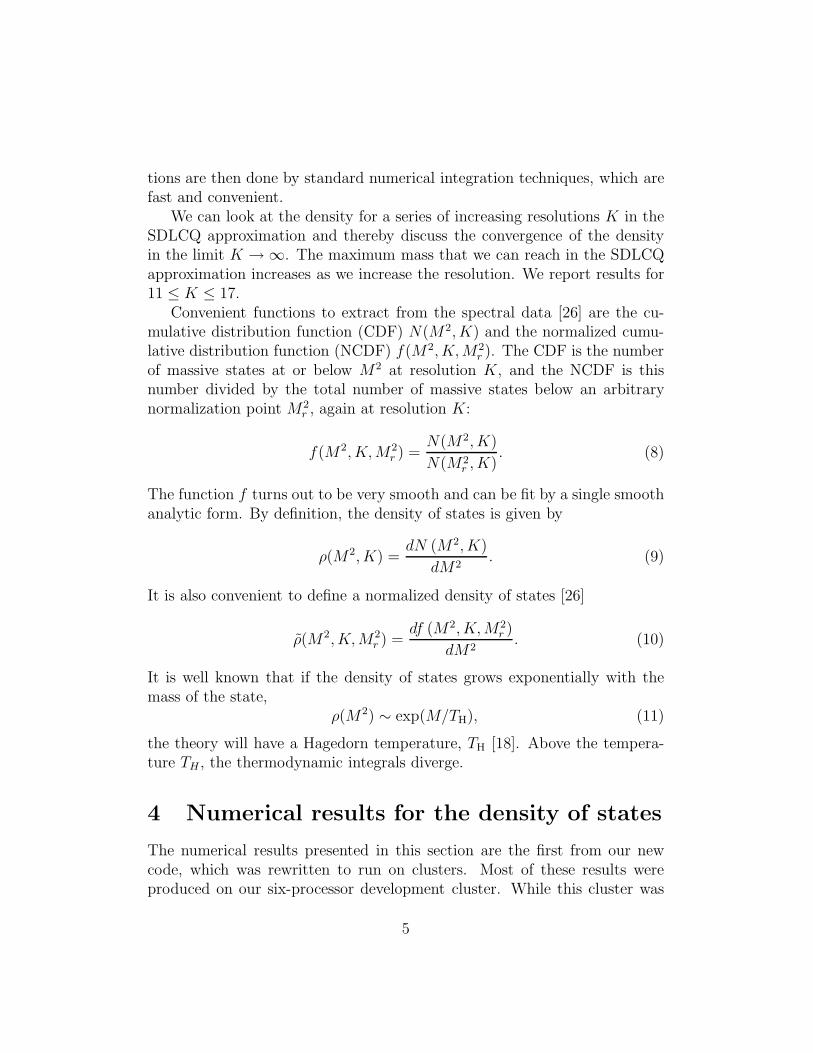
Figure 1: The distribution functions (a) N(M2, K) for K = 12 and (b)f(M2, K, 100) for K = 12, 14, and 17, as functions of M2 in units of g2Nc/π.In (a) we also show the error-function fit a erf(b(x − c)) + d, and in (b), apolynomial fit.

In the SDLCQ approximation, the portion of the spectrum that we cansee at any finite resolution will naturally be cut off. As we approach thecutoff, the approximation limits the number of states that are available anddistorts the density of states. In Fig. 1a, we present the data for the CDFat resolution K = 12, where we can diagonalize the entire Hamiltonian.We clearly see evidence of this distortion. By the midpoint, the cutoff isalready diminishing the number of states available in the approximation.Interestingly, we can find a fit to this data with a simple universal functionof the form a erf(b(x − c)) + d. Clearly the fit shown is excellent; the fit isso good that one cannot separately see the data and the fitted curve on thisscale.

6

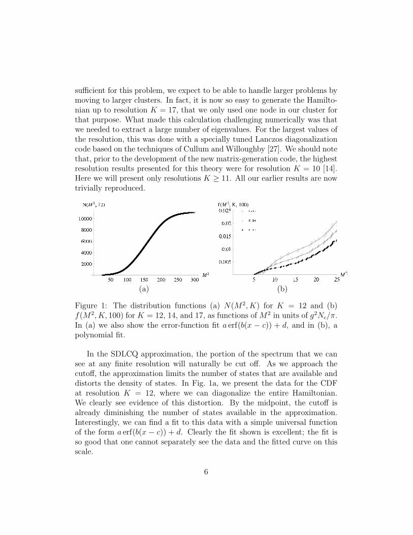
(a) (b)

Figure 2: The normalized density of states (a) for M2 ≤ 100 and (b) extrap-olated to all masses. The data points are a convenient way of displaying thecontinuous functions calculated from the fits to the CDF.

At low masses, there is a mass gap, which has been discussed elsewhere [5].The mass gap closes linearly with 1/K. For very small values of M2, thedecrease of the mass gap with increasing resolution adversely affects thequality of the universal fit, and it is convenient in that region to improve thequality of the fit by using a polynomial function of the form

f(x,K, 100) =p(K)∑

p=0

αp xδK+pΘ(x− xmin(K)). (12)

In Fig. 1b we show the fit to the NCDF for some representative values of theresolution K. We have only shown the data at resolutions K = 12, 14, and17 to keep the figure uncluttered. One can see how the endpoints tend tolower values as the mass gap closes with increasing K.

At larger values of K it is difficult to completely diagonalize the entireHamiltonian. We have limited ourselves to states with M2 ≤ 100. However,once we know the universal form of the function that fits the CDF, we canfit just the region M2 ≤ 100 and extrapolate to all masses. At large M2,the CDF approaches the total number of bound states. The total number ofstates in the SDLCQ approximation at any resolution, and, in any symmetrysector in the large-Nc approximation, is exactly calculable; the general resultswill be discussed elsewhere. We use this asymptotic value of the CDF, inaddition to the behavior for M2 ≤ 100, in making the fits. We have donethis at all resolutions up to K = 17. In Fig. 2a we show the normalizeddensity of states calculated from the NCDF, for M2 ≤ 100. In Fig. 2b we

7

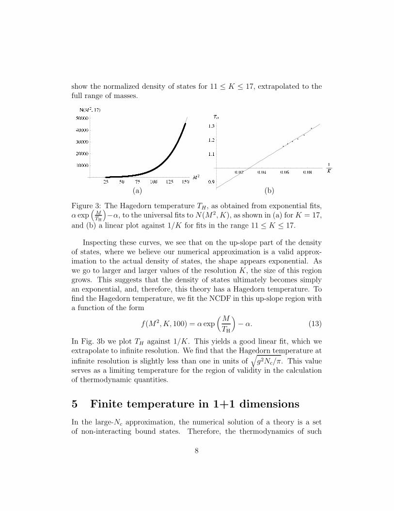
show the normalized density of states for 11 ≤ K ≤ 17, extrapolated to thefull range of masses.

(a) (b)

Figure 3: The Hagedorn temperature TH , as obtained from exponential fits,α exp

(

MTH

)

−α, to the universal fits to N(M2, K), as shown in (a) forK = 17,

and (b) a linear plot against 1/K for fits in the range 11 ≤ K ≤ 17.

Inspecting these curves, we see that on the up-slope part of the densityof states, where we believe our numerical approximation is a valid approx-imation to the actual density of states, the shape appears exponential. Aswe go to larger and larger values of the resolution K, the size of this regiongrows. This suggests that the density of states ultimately becomes simplyan exponential, and, therefore, this theory has a Hagedorn temperature. Tofind the Hagedorn temperature, we fit the NCDF in this up-slope region witha function of the form

f(M2, K, 100) = α exp(

M

TH

)

− α. (13)

In Fig. 3b we plot TH against 1/K. This yields a good linear fit, which weextrapolate to infinite resolution. We find that the Hagedorn temperature at

infinite resolution is slightly less than one in units of√

g2Nc/π. This valueserves as a limiting temperature for the region of validity in the calculationof thermodynamic quantities.

5 Finite temperature in 1+1 dimensions

In the large-Nc approximation, the numerical solution of a theory is a setof non-interacting bound states. Therefore, the thermodynamics of such

8

supersymmetric theories is simply the thermodynamics of a gas of a largenumber of species of degenerate bosons and fermions. In principle, one couldgo beyond the calculation of the standard set of the thermodynamic functionsand calculate a variety of matrix elements. These calculations would requirethe wave functions of the bound states, which can be calculated as part of theSDLCQ calculation. We will, however, not exploit this detailed informationhere. We will focus on the calculation of standard thermodynamic quantitiesthat can be obtained from the density of states. The light cone plays norole beyond the calculation of the density; the thermodynamics is that of asystem at rest.

Let us now briefly review the thermodynamics of free bosons and fermions.We assume that our system has constant volume V and is in contact with aheat bath of constant temperature T . The free energy in units with kB = 1is

F(T, V ) = −T lnZ. (14)

The contribution of a single bosonic oscillator to the free energy FB is

FB = 2V T∫ ∞

0

dp3

2πln(

1 − e−p0/T)

, (15)

where p0 =√

M2 + p23 and the factor of 2 compensates for integrating over

only positive values of p3. It is convenient to change variables from p3 to p0:

dp3 =p0

√

p20 −M2

dp0. (16)

The limits of integration are changed from 0 ≤ p3 <∞ to M ≤ p0 <∞. Wemay also use the following representation for the logarithm that appears inthe integrand

ln(

1 − e−p0/T)

= −∞∑

j=1

e−jp0/T

j, (17)

since p0 is positive and 0 ≤ e−p0/T < 1. Finally, we obtain an expression forthe total bosonic free energy just by summing over the energy spectrum

FB = −V Tπ

∞∑

n=1

∞∑

j=1

∫ ∞

Mn

dp0p0

√

p20 −M2

n

(

e−jp0/T

j

)

. (18)

The calculation of the fermionic contribution to the free energy proceedsanalogously, and we find the identical result with the exception that there is

9

a factor of (−1)j inside the summation. We can separate out the masslessstates from these expressions and calculate their contribution explicitly. Weknow that for resolution K there are (K − 1) massless bosons and (K − 1)massless fermions. Thus the contribution to the free energy from masslessstates is

F0B = −(K − 1)π

6V T 2, F0

F = −(K − 1)π

12V T 2. (19)

After doing the integral over p0, we find for the total free energy

F(T, V )

V T 2= −(K − 1)π

4− 2

Tπ

∞∑

n=1

∞∑

l=0

Mn

K1

(

(2l + 1)Mn

T

)

(2l + 1). (20)

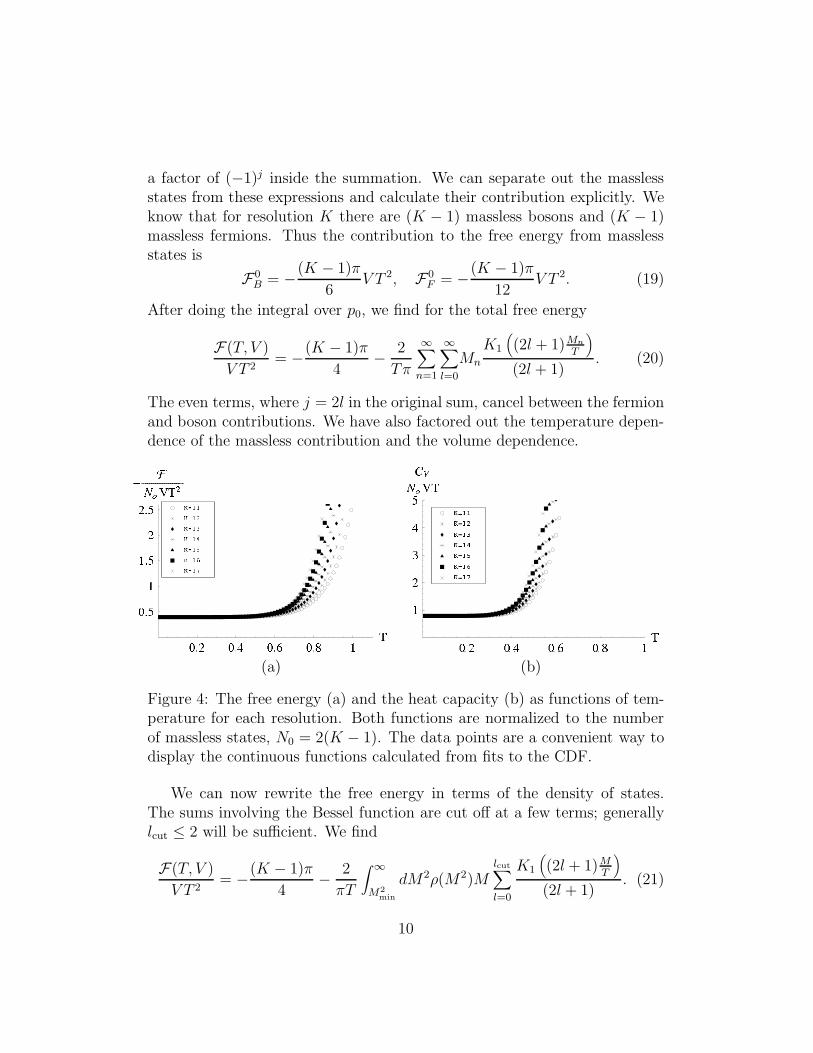
The even terms, where j = 2l in the original sum, cancel between the fermionand boson contributions. We have also factored out the temperature depen-dence of the massless contribution and the volume dependence.

(a) (b)

Figure 4: The free energy (a) and the heat capacity (b) as functions of tem-perature for each resolution. Both functions are normalized to the numberof massless states, N0 = 2(K − 1). The data points are a convenient way todisplay the continuous functions calculated from fits to the CDF.

We can now rewrite the free energy in terms of the density of states.The sums involving the Bessel function are cut off at a few terms; generallylcut ≤ 2 will be sufficient. We find

F(T, V )

V T 2= −(K − 1)π

4− 2

πT

∫ ∞

M2min

dM2ρ(M2)Mlcut∑

l=0

K1

(

(2l + 1)MT

)

(2l + 1). (21)

10

The free energy may now be used to calculate all the thermodynamicfunctions. The internal energy and heat capacity are given by,

E(T, V ) = T 2

(

∂lnZ

∂T

)

V

, CV(T, V ) =

(

∂E∂T

)

V

. (22)

It is straightforward, given the density of states, to calculate the thermo-dynamic functions. Fig. 4a shows the free energy, and Fig. 4b shows the heatcapacity. We expect the free energy to diverge as N2

c and therefore mustnormalize our results to extract a finite number. In most of the region belowthe Hagedorn temperature the thermodynamic functions are totally domi-nated by the massless states. It therefore seems appropriate to normalizethe thermodynamic functions to the total number of massless bound states,which is a function of the resolution and is 2(K−1). Alternatively, we couldnormalize by the number of states in any region. It is conceivable that at veryhigh resolutions, where the mass gap is significantly less than one, that themassive states may make an important contribution to the thermodynamics.In that case we would not choose to normalize by the massless states.

6 Discussion

The large-Nc SDLCQ solution of N = (1, 1) super Yang–Mills theory in1+1 dimensions gives a set of non-interacting bound states. From this set ofbound states it is in principle possible to calculate the thermodynamics of thistheory. Central to this calculation is the calculation of the density of states.At resolutions K = 12 and below, where we can completely diagonalize theHamiltonian, we find that the entire cumulative distribution function can befit with a single erf function. From the cumulative distribution function, itis straightforward to calculate the density of states. For K larger than 12,it is difficult to calculate the entire spectrum; therefore, our calculations areconfined to a fixed range of masses, M2 ≤ 100 g2Nc/π. Using the knownform of the distribution, we only need to fit a section of the cumulativedistribution function to get a very good fit to the entire distribution. Weknow analytically the total number of bound states at any resolution, andthis information can also be used in conjunction with a fit to a section of thedistribution to produce the fit to the entire distribution.

The density of states that are found by this procedure grow sharply atsmall masses, then level off and decrease at larger masses. The peak of the

11

density of states grows as we increase the resolution. Our understandingof this behavior is that the cutoff of the theory is forcing the density ofstates to level off, turn over, and then decrease. The true behavior of thedensity of states is reflected in the region of the density of states that israpidly increasing, because it is this region that is increasing in size with theresolution K.

It appears that the cumulative distribution function, and, therefore, thedensity of states, are growing exponentially with the mass. To confirm thisand find the asymptotic values of this growth, we fit the cumulative distri-bution function with an exponential at each K. We extrapolate these resultsto infinite resolution to find the asymptotic behavior of the density of states.The coefficient of the exponential growth is the reciprocal of the Hagedorn

temperature. We find that this temperature is about 0.854√

g2Nc/π/kB.The thermodynamic functions calculated from this data are expected to pro-duce valid results up to a temperature that is around TH.

It is now straightforward to calculate a standard set of thermodynamicfunctions from this density of states. The best estimate of the thermodynam-ics is obtained by using the exponential fits to the density of states. Whatwe see is that, for resolutions up to K = 17, all of the massive bound statesare well above the Hagedorn temperature. The thermodynamics below THis therefore controlled by the K − 1 massless boson bound states and K − 1massless fermion bound states.

We can speculate on what will happen as the resolution goes to infinity.We have seen that the mass gap closes linearly with 1/K. So, for a reso-lution of order 100, there will be massive bound states below the Hagedorntemperature. This, of course, assumes that the estimate of the Hagedorntemperature is not changed by the higher resolution calculations. We found,however, that the actual number of massive bound states in a fixed massrange may grow slowly. For resolutions 11 to 17 we are able to find excellentfits with both exponential and linear growth as a function of the resolutionK for masses with M2 ≤ 100. If the number of massive states grows onlylinearly with K, the contribution to the thermodynamic functions below THmight become significant but not dominant.

These calculations indicate that N = (1, 1) super Yang–Mills theoryin 1+1 dimensions has a Hagedorn temperature of about one in units of√

g2Nc/π/kB. More generally, we found that SDLCQ can be used to find in-teresting properties of finite-temperature supersymmetric field theories. The

12

extension of this method to theories with more supersymmetry and in higherdimensions appears to be straightforward but may be computationally chal-lenging.

Acknowledgments

This work was supported in part by the U.S. Department of Energy and bythe Minnesota Supercomputing Institute.

References

[1] S. S. Gubser, I. R. Klebanov, and A. W. Peet, Phys. Rev. D 54, 3915(1996) [arXiv:hep-th/9602135].

[2] M. Li, JHEP 9903, 004 (1999) [arXiv:hep-th/9807196]; A.A. Tseytlinand S. Yankielowicz, D3-brane Nucl. Phys. B 541, 145-162 (1999)[arXiv:hep-th/9809032]; A. Fotopoulos and T.R. Taylor, at finite tem-perature,” Phys. Rev. D 59, 061701 (1999) [arXiv:hep-th/9811224].

[3] A. Das and M. Kaku, Phys. Rev. D 18, 4540 (1978).

[4] Y. Matsumura, N. Sakai, and T. Sakai, Phys. Rev. D 52, 2446 (1995)[arXiv:hep-th/9504150].

[5] O. Lunin and S. Pinsky, AIP Conf. Proc. 494, 140 (1999)[arXiv:hep-th/9910222].

[6] A. G. Cohen, D. B. Kaplan, E. Katz, and M. Unsal,[arXiv:hep-lat/0302017]; A. Feo, to appear in the proceedings ofthe 20th International Symposium on Lattice Field Theory (LATTICE2002), Boston, Massachusetts, 24-29 Jun 2002, [arXiv:hep-lat/0210015];I. Montvay, Nucl. Phys. B 466, 259 (1996) [arXiv:hep-lat/9510042].

[7] S. J. Brodsky, Nucl. Phys. Proc. Suppl. 108, 327 (2002)[arXiv:hep-ph/0112309].

[8] V. S. Alves, A. Das, and S. Perez, Phys. Rev. D 66, 125008 (2002)[arXiv:hep-th/0209036]; A. Das and X. X. Zhou, Phys. Rev. D 68,065017 (2003) [arXiv:hep-th/0305097]; A. Das, arXiv:hep-th/0310247.

13

[9] H. A. Weldon, Phys. Rev. D 26, 1394 (1982); 67, 085027 (2003)[arXiv:hep-ph/0302147]; 67, 128701 (2003) [arXiv:hep-ph/0304096].

[10] M. Beyer, S. Mattiello, T. Frederico, and H. J. Weber,[arXiv:hep-ph/0310222].

[11] S. Elser and A. C. Kalloniatis, Phys. Lett. B 375, 285 (1996)[arXiv:hep-th/9601045].

[12] H.-C. Pauli and S.J. Brodsky, Phys. Rev. D 32, 1993 (1985); 32, 2001(1985);

[13] S.J. Brodsky, H.-C. Pauli, and S.S. Pinsky, Phys. Rep. 301, 299 (1998)[arXiv:hep-ph/9705477].

[14] F. Antonuccio, O. Lunin, and S. S. Pinsky, Phys. Lett. B 429, 327 (1998)[arXiv:hep-th/9803027]. F. Antonuccio, O. Lunin, and S. Pinsky, Phys.Rev. D 58, 085009 (1998) [arXiv:hep-th/9803170].

[15] F. Antonuccio, O. Lunin, and S. Pinsky, Phys. Rev. D 59, 085001 (1999)[arXiv:hep-th/9811083].

[16] P. Haney, J. R. Hiller, O. Lunin, S. Pinsky, and U. Trittmann, Phys.Rev. D 62, 075002 (2000) [arXiv:hep-th/9911243].

[17] J. R. Hiller, S. Pinsky, and U. Trittmann, Phys. Rev. D 64, 105027(2001) [arXiv:hep-th/0106193].

[18] R. Hagedorn, Nuovo Cimento Suppl. 3, 147 (1965); R. Hagedorn, NuovoCimento 56A, 1027 (1968).

[19] D. Kutasov, Phys. Rev. D48, 4980 (1993) [arXiv:hep–th/9306013].

[20] F. Antonuccio, O. Lunin, S. Pinsky, and S. Tsujimaru, Phys. Rev. D60, 115006 (1999) [arXiv:hep-th/9811254].

[21] J. S. Rozowsky and C. B. Thorn, Phys. Rev. Lett. 85, 1614 (2000)[arXiv:hep-th/0003301].

[22] S. Salmons, P. Grange, and E. Werner, Phys. Rev. D 65, 125014 (2002)[arXiv:hep-th/0202081].

14

[23] T. Heinzl, arXiv:hep-th/0310165.

[24] A. Harindranath, L. Martinovic, and J. P. Vary, Phys. Lett. B 536, 250(2002); V. T. Kim, G. B. Pivovarov, and J. P. Vary, Phys. Rev. D 69,085008 (2004) [arXiv:hep-th/0310216].

[25] D. Chakrabarti, A. Harindranath, L. Martinovic, and J. P. Vary, Phys.Lett. B 582, 196 (2004) [arXiv:hep-th/0309263].

[26] O. Lunin and S. Pinsky, Phys. Rev. D 63, 045019 (2001)[arXiv:hep-th/0005282].

[27] J. Cullum and R.A. Willoughby, in Large-Scale Eigenvalue Problems,eds. J. Cullum and R.A. Willoughby, Math. Stud. 127 (Elsevier, Ams-terdam, 1986), p. 193.

15