Centro V. VolterraUniversita di Roma Tor Vergata

1

Yang–Mills equations and Levy-laplacians

Luigi Accardi

30 luglio 2015

Sommario

We discuss some recent developements concerning the Levy lapla-cian: its connections with the Yang–Mills equations, with the II1–factor, with the singular traces of Dixmier type; the associated classi-cal and quantum Brownian motion and Ornstein–Uhlenbeck process;various approximation properties for the process itself and the as-sociated semigroup; spectral properties; Cameron–Martin–Girsanovformulae; Dirichlet forms; ...

1 (0.) Introduction

The present work reports on a line of research motivated by quantumprobability and begun in collaboration with Igor Volovich, Paolo Gi-bilisco, Lu Yun Gang and developed in collaboration with the sameauthors and with Oleg G. Smolyanov, Paolo Roselli, Nobuaki Obata,Vladimir Bogachev. The main results obtained along this line are thefollowing.

The starting point is the result that a parallel transport is asso-ciated to a connection satisfying the (euclidean) Yang–Mills equationsif and only if, when considered as a functional defined on the spaceof piecewise smooth paths, it is an harmonic function for the Levylaplacian, i.e. it satisfies the corresponding Laplace equation [AcGi-Vo1], [AcGiVo2]. This fact, together with the derivation propertyof the Levy laplacian, provides an algebraic tool to obtain new solu-tions of the YM equations by composing previously known solutions.The proof of this result has lead to the introduction of an infinite

2

hierarchy of exotic Laplacians, generalizing the Levy Laplacian, andtherefore to a remeditation of the very notion of laplacian (in infinitedimensions). The result of this is the proposal to set up a one-to-onecorrespondence between laplacians and traces on ∗-algebras of opera-tors [AcSmo1]: the Volterra laplacian corresponds to the trace classoperators; the Levy laplacian to the hyperfinite II1–factor [AcOba2];the exotic laplacians, to ∗-algebras of unbounded operators with exo-tic traces. The analogue, for exotic laplacians, of the characterizationof the Levy laplacian as ergodic average of the second derivatives, isestablished [Ros]. Several examples are discussed.

An existence and uniqueness theorem for the heat equation asso-ciated to the Levy laplacian is proved by means of an explicit formulafor its fundamental solution. The associated Levy heat semigroup isused to construct a classical Markov process called the Levy Brownianmotion [AcRoSmo].

The corresponding Ornstein–Uhlenbeck process is constructed bya finite dimensional approximation procedure and associated to a Diri-chlet form which is intrinsically infinite dimensional, in the sense thatit vanishes identically on the cylindrical functions [AcBo].

The notions of Levy trace and Levy determinant are introduced(the latter illustrates the general theory of determinants in von Neu-mann algebras due to Fuglede and Kadison [FuKa] – cf. also [Arv])and used to prove a trace formula for gaussian measures which, incase of adapted processes, generalizes the Cameron–Martin–Girsanovformula [AcSmo2].

A Fock space realization of the Levy Brownian motion is obtai-ned and this allows to construct the corresponding quantum process[AcOba2].

2 (1.) The Yang–Mills equations

In the following we shall use the term manifold as equivalent of smoothmanifold; map as equivalent of smooth map, . . .

Definition 1 Let V be a vector space. A vector bundle H over Mwith fiber V is a triple:

H, π,M ≡ H

such that

3

i) H,M are manifolds.

ii) π : H →M is a surjective map.

iii) For each x ∈ M there is an open set U ⊆ M , containing x, andan isomorphism (also called a local frame or a fiber coordinate)

gU (x) : V → Hx := π−1(x) ⊆ H

such that the map (ξ, x) ∈ V ×M 7→ gU (x)ξ ∈ H is smooth.

In the case of interest for us, in the following, V shall be a (real orcomplex) Hilbert space and each gV (x) a unitary isomorphism. Thesections are the maps S : M → H such that

π S = idM

The family of all sections shall be denoted

C(H) ≡ C(M ; H)

In the following we shall assume that M is an orientable RiemannianManifold and that H π→ M is an Hilbert bundle with N–dimensionalfiber Ho = V .

Definition 2 A covariant derivative 5 on H, is a map 5 : TM ×C(H)→ H such that

• i) 5 is local, i.e. for any section S:

5(TxM,S) ⊆ Ex ; ∀x ∈M

• ii) 5 is bilinear. We shall use the notation

5(v, S) =: 5vS

• iii) 5 satisfies the Leibnitz rule

5v(f · S)(m) = v(f) · S(m) + f(m)5v S

A local frame g ≡ (g(x), x ∈ U) identifies sections S to functionsξ : M → V by:

g(x)−1S(x) =: ξ(x)

4

In this identification, the covariant derivative is identified to a mapfrom vectors at x ∈ M to linear operators on V . More precisely, ifg(x)−1S(x) = ξ(x), then

5vS = g(x)[< dξ, v > + < Ag, v > ξ(x)] ; v ∈ TxM

which we write symbolically

5 = d+A , A =∑j

Aj(x)dxj , Aj ∈ Lie(SU(N))

where d is the exterior derivative. The matrix Ag is called the connec-tion matrix or the potential associated to the covariant derivative5. For any curve:

σ : [0, 1]→M ; σ(o) = x ∈M

there exists a unique map

s ∈ [0, 1] 7→ U5gs (σ) ∈ Iso (V )

characterized by the following property. For any local frame g, U5,gs (σ)is the unique solution of the equation:

d

dsU5,gs (σ) = − < Ag(σs), σ > U5,gs (σ) ; U5,go (σ) = idHx

The covariance property

U5,g′g

s (σ) = g(x)U5,g′

s (σ)g(xs)−1

shows that there exists a unique 1–parameter family of maps U5s (σ) ∈Iso(Hx, Hσs) which, in the local frame g, coincides with U5,gs (σ), for

each local frame g. The map U5s (σ) is called the parallel transportalong σ. In the following, we shall define

Loopx(M) = σ : [0, 1]→M : σ(0) = σ(1) = x

To every connection matrix A we associate its curvature F =(formally) 5A = dA+ [A,A]:

Fµν = ∂µAν − ∂νAµ − [Aµ, Aν ] = dA+A ∧A

The Yang Mills Equations are:

5

5∗F = 0⇐⇒ d(∗F ) + [A, ∗F ] = 0

where ∗ denotes the Hodge involution. In coordinates:

5λFλµ = 0

where 5λ := 5µgµλ and g = (gµν) denotes the metric tensor.

The self dual connections are characterized by the condition ∗F = F .For such connections the Yang–Mills equations become equivalent todF + [A,F ] = 5F = 0, which is the Bianchi identity. So, for selfdual connections, the Yang–Mills equations are identically satisfied.This means that the description of the space of self-dual connectionssatisfying some smoothness conditions is equivalent to the descriptionof a subclass of solutions of the Yang–Mills equations with correspon-ding regularity properties. In [AHDM] it was shown that the space ofself-dual connections is a manifold whose dimension can be expressedby topological invariants of the bundle H.

From the analytical point of view this geometric approach has twomain limitations:

• - It gives scarse information on non self-dual solutions

• - Only very smooth solutions can be dealt with.

Moreover the unknown, in the equations, is the connection matrix A,which is not a geometrical i.e. intrinsic (physical) object as opposedto F or to the parallel transport associated to the connection matrix.

Under regularity conditions (which we shall not specify here), toevery connection form one can associate a parallel transport and con-versely. The correspondence which to every potential A = (Aµ) asso-ciates its parallel transport, is called the path ordered exponential. Insymbols:

A ≡ (Aµ(x))→ Uγ = P exp

∫γA = P exp

∫ 1

oAµ(γs)γsds (1)

where the right hand side of (1.1) is defined by the iterated series.So, under regularity conditions, to assign a potential A ≡ (Aµ) isequivalent to assign a functional U on the paths (continuous curves)on the space time

U : γ ∈ Paths(M)→ Uγ ∈ n× n Matrices

6

Moreover, by Driver’s Theorem, having fixed an isomorphism: uo :V → Hx

u−1o U5(σ)uo := U(σ) ; U : σ ∈ Loopx(M)→ U(σ) ∈ GL(V )

one can establish an equivalence

H,5 ←→ U : Loopx(M)→ GL(V )

between pairs H,5 (bundle–connections pairs) and maps U : Loopx(M)→GL(V ) satisfying

• - U(στ) = U(σ)U(τ)

• - U is parametrization invariant

• - U is strongly continuous

In other words:

Theorem 1 [Driver] The restriction of the parallel transport on loops(more precisely the maps U) allows to reconstruct both:

• - the bundle H

• - the covariant derivative 5 uniquely up to isomorphisms if U isstrongly continuous.

This suggests the programme of an invariant formulation of the Yang-Mills equations based on the notion of parallel transport. This pro-gramme has a long history which has been reviewed in [AcGiVo2]where the following theorem has been proved:

Theorem 2 Let Ω be the space of piecewise smooth paths [0, 1] →Rn and let U : γ ∈ Ω→ U(γ) ∈ GL(d,C) be a parallel transport anddenote Fλµ the associated curvature tensor (c.f. Section of (4.) ). Thefollowing statements are equivalent:

• (i) The curvature tensor Fλµ satisfies the (euclidean) Yang Millsequations

5λFλµ = 0 (2)

• (ii) The functional U satisfies the Laplace equation

∆LU(γ) = 0 (3)

where ∆L denotes the Levy laplacian.

7

In [AcGiVo2] only the euclidean, flat case has been considered, ho-wever the techniques developed by Driver [Driv2] allow to extend theresult to manifolds. From a formal point of view there is no differencebetween the derivation for the Levy laplacian and the Levy D’Alam-bertian (cf. [AcGivo]), therefore also the rstriction to the euclideanregion does not seem to be essential.

Notice that, in the above statement of the theorem, there is nodistinction between self–dual and non self–dual solutions, in fact acharacterization of self–dual solution in terms of parallel transportseems to be missing at the moment. This suggests that the invariantformulation of the YM equations could be used to study non self–dualsolutions. Moreover the connection between probability theory andpotential theory, well known and widely studied in the case of theclassical laplacian, suggests a probabilistic approach to the study ofthe potential theory for the Levy laplacian.

More precisely, a natural heuristic idea to find nontrivial solutionsUγ of the Levy Laplace equation

∆LUγ = 0

is to exploit the starting point of the probabilistic approach to poten-tial theory, i.e. the correspondence

∆LU = 0⇐⇒ et∆LU = U

between harmonic functions for a laplacian and fixed points of thecorresponding Markovian semi–group. This leads to the study of thesolutions of the heat equation

∂tut = ∆Lu ; u(o, x) = uo(x)

and of the corresponding Brownian motion, in the hope that this mightyield informations on solutions of the Laplace equation (more generallyon the spectrum of ∆L).

The choice of a space where ∆L is defined corresponds to the choiceof a boundary condition.

The first step of such a program is the consruction of the Brownianmotion for the Levy laplacian and the study of its properties. In thefollowing sections some recent progresses in this direction are reported.

8

3 (2.) Heuristic introduction to the

Levy laplacian

An intuitive way to introduce the Levy laplacian is to think of it asthe generator of an infinite dimensional diffusion process, obtainedas a limit of finite dimensional diffusions whose diffusion coefficientare inversely proportional to the space dimension. More concretely,consider an orthonormal basis (ej) in Rn. Then the n–dimensionallaplacian in the coordinates detemined by that basis looks like:

∆n =∂2

∂x21

+ . . .+∂2

∂x2n

(4)

and the associated diffusion, with diffusion coefficient 1/n is

∂

∂tψt = − 1

n∆nψt (5)

As n tends to infinity, Rn approximates a separable Hilbert space H,with an orthonormal basis (ej) and the formal limit of equation (2.2)looks like

∂

∂tψt = −limn→∞

1

n

n∑n=1

∂2

∂x2j

ψt (6)

The formal differential operator at the right hand side of (2.3), i.e.

∆L := limn→∞1

n

n∑j=1

∂2

∂x2j

(7)

is the so called the Levy laplacian on H, associated to the orthonormalbasis (ej).

The rigorous theory of the Levy laplacian has been developed byT. Hida and his school, and is strictly related to notion such as whitenoise calculus, Hida distributions, . . .. For the moment I shall notdiscuss the rigorous theory, but I limit myself to an heuristic remark:a particle performing a diffusion, for example a Brownian particle,can be thought of a a particle whose trajectory is perturbed by somenoise: the noise is so much larger as the diffusion coefficient is larger.Thus, if the diffusion coefficient decreases as 1

n we expect that thenoise decreases with the number of dimensions and that the in limitone should expect a kind of deterministic behaviour. This intuition is

9

confirmed, in an abstract way by the so-called derivation property ofthe Levy laplacian:

∆L(f.g) = (∆Lf) · g + f(∆Lg) (8)

which formally implies that the associated semigroup is a semigroupof automorphisms of the algebra of the smooth functions on H.

We shall see that this derivation property shall yield some nontri-vial information on the structure of the solutions of the Yang Millsequations, at least of those solutions which are smooth enough forproperty (2.5) to hold (cf. Section (3.) below).

Also from the point of view of quantum mechanics the Levy lapla-cian has a natural interpretation: interpreting the qj , pj operators asrelated to the degrees of freedom of a quantum system (e.g. a gas ora field), one has that

p2j = − ∂2

∂x2j

represents the kinetic energy of the j −−th particle (unit mass is as-sumed). Thus the Levy laplacian can be interpreted as kinetic energydensity of a system with infinitely many degrees of freedom.

4 (3.) An algebraic structure on the

solutions of the Yang–Mills equations

Before giving a closer look at the solutions of the (Levy) Laplaceequation, we shall discuss an interesting consequence of the possibilityof formulating the Yang–Mills equations as a (Levy) Laplace equation,Following the approach of [AcGi1], we look at parallel transports as

representations of the groupoid of curves on a manifold (better: onthe diffeomorphisms group of the manifold). Being representations itmakes sense to speak of their tensor product and, from the derivationproperty of the Levy laplacian, one easily deduces that

∆L(Uγ ⊗ Vγ) = ∆LUγ ⊗ Vγ + Uγ ⊗∆LVγ

It follows that the tensor product of two solutions is still a solution.Thus, even if the Yang–Mills equations are nonlinear, there is a na-tural structure of ring on the family of their solutions (with sufficientsmoothness). Clearly the direct sum (tensor product) of two solutions

10

shall live on the direct sum (tensor product) of the correspondingbundles. If we want to use this remark to construct new solutions ofthe Yang–Mills equations, on a given single bundle, out of given ones,it is convenient to introduce the notion of an irreducible solution ofthe Yang–Mills equation. This can be done as follows (we discuss onlythe case of Rn).

By Driver’s theorem [Driv], a parallel trasport is uniquely deter-mined by its restriction to the loops. Therefore we can restrict ourattention to the loops starting at the origin in Rn. They form a groupunder concatenation and path reversal: the loop group (at the ori-gin) denoted Loopo (Rn). By standard arguments the loop groups atdifferent points are isomorphic, whenever the path space contains suf-ficiently many curves to connect 2 arbitrary points in Rn. The imageof the loop group under a parallel transport is called the holonomygroup of the parallel trasport and denoted Hol (U). If the fiber at theorigin is identified to Cd, then Hol (U) becomes identified to a sub-group of SU (d). Let Ho (U) denote the closure of this subgroup: it isa compact subgroup of SU (d).

Consequently (and in obvious notations) Hol (U)⊗Hol (V ) isa compact sub-group of SU(dU )⊗ SU (dV ) (where dU and dV denoterespectively the dimensions of the representations U and V ).

We can therefore write CdU ⊗CdV as a direct sum of irreduciblesubspaces

CdU ⊗CdV = ⊕mj=1Kj

where Kj is isomorphic to Cdj and d1 + · · ·+ dm = dU · dV .By construction, for any loop γ at the origin in Rn, any of the

subspaces Kj gives a representation of the loop group on Kj , which

shall be denoted Wjo (j = 1, · · · ,m).

Repeating the above argument for every point x ∈ Rn, we obtaina new Hilbert bundle Kj : this follows immediately from the isomor-phism of the groups Hol x (U) for all x ∈ Rn. Since they are clearlycontinuous, because U an V are supposed to be such, we can applyDriver’s theorem and deduce the existence of a parallel transport stilldenoted Wk, on the bundle Kj . Finally, let us denote

Pj : CdU ⊗CdV −→ Kj

the orthogonal projection. Then clearly

∆LPj = Pj∆L

11

and therefore, for any γ in the loop group

∆LWjγ = ∆LPjUγ ⊗ VγPj = Pj∆L(Uγ ⊗ Vγ)Pj = 0

Therefore each Wj defines a connection satisfying the Yang–Millsequations. Summing up, the above discussion suggests to introducethe following definition:

Definition 3 A solution of the Yang–Mills equation is called irredu-cible if the associated parallel transport has an irreducible holonomyrepresentation.

Given two irreducible solutions of the Yang–Mills equations which cor-respond to the same dimension d of the fiber, one can decompose thetensor product U ⊗ V into irreducibles. If among these ones there isexactly one of dimensions d, then we say that the associated connec-tion is obtained by composition from the connections associated to Uand V .

For a general gauge group, such a composition law need not to bedefined, either because in the decomposition of U⊗V into irreducibles,there might be no term of dimension d, or, because there might bemore than one. However, for special choices of the gauge group thecomposition law might be defined for any pairs of irreducibles.

5 (4.) Lebesgue-free approach to the

heat equation

As a motivation for our approach, we shall rephrase the finite di-mensional scalar case in such a way that the infinite dimensionalgeneralization becomes quite natural.

Starting from

∂tψ(t, x) =1

n∆nψ(t, x) ; ψ(o, x) = ψo(x)

and taking the x–Fourier transform of both sides we find:

∂tψ(t, k) = − 1

nk2ψ(t, k) ; ψ(o, k) = ψo(k) (9)

12

where ϕ denotes Fourier transform with respect to the Lebesgue mea-sure

F+ϕ(k) = ϕ(k) =

∫ei<k,x>ϕ(x)dx ; x ∈ Rn

The obvious solution in Fourier space is:

ψ(t, k) = e−tk2n ψo(k) ; k2 =

n∑j=i

k2j

Going back to the x–space by inverse Fourier transform one finds

ψ(t, x) = [F−1ψ(t, ·)](x)

The correspondence

F+ : Functions −→ Functions

requires a privileged (Lebesgue) measure and it is difficult to invertin the ∞–dimensional case where there is no such measure. The factthat the intrinsic correspondence is:

F+ : Measures −→ Functions

whose inversion in∞–dimensions is controlled by theorems of KSMG(Kolmogorov - Sazonov - Minlos - Gross)–type, suggests that, in ∞-dimensions, equation (4.1) should be interpreted as an equation onmeasures.

6 (5.) Exotic laplacians

The usual laplacian is the trace of the second derivative. This suggeststhat to every trace one should associate the corresponding laplacianand this leads to a natural connection between the theory of von Neu-mann algebras and infinite dimensional analysis. The framework ofvon Neumann algebras however is too narrow to include several in-terestin examples, which involve unbounded operators, therefore in[AcSmo1] the following notion of laplacian was introduced.

Definition 4 Let H be a Hilbert space; A a ∗-algebra of operatorsdefined on a common invariant subspace HV ⊆ H ; τ a trace on A.Denote

CnA(H) ; n ∈ N ∪ ∞ (10)

13

the space of Cn - functions f : H → R such that for each x ∈H, f ′′(x) ∈ A. For each f ∈ C2

A(H), the (A, τ)-laplacian (sometimessimply called the τ -laplacian ) of f is defined by:

∆A,τf(x) = ∆τf(x) = τ(f ′′(x)) ; ∀x ∈ H (11)

The following example shows that there are natural traces on alge-bras of differential operators and also corrects an error contained inTheorem (4.8) in [AcSmo1] (there is only one natural trace on thealgebra described in the example below, and not infinitely many, aserroneously stated in [AcSmo1]). Example(5.2) Let Ao denote thealgebra of compact operators on H = L2(R) and A1 the algebra ofmultipication by C∞–functions. The algebraic direct sum

A := ⊕n≥oAn = Ao ⊕A1 ⊕A1∂ ⊕ . . .⊕A1∂n ⊕ . . . (12)

is a ∗-algebra and the sum in (5.3) is direct. A simple computationshows that the linear functional τ on A, defined by

τ(ao +

∞∑n=1

an∂n−1) :=

∫Ran(s)ds ; n ≥ 1 (13)

where n is the largest integer such that an 6= 0, is a trace on A.

The example above is strictly related to another natural class ofexamples of nonstandard laplacians which can be constructed by con-sidering function whose second derivatives are operators with an in-tegral kernel which can be decomposed in a unique way as a sum ofincreasingly singular distributions. The usual laplacian shall corre-spond to the case when the second derivative is trace class; the Levylaplacian, to the case when the second derivative is a trace class plusa multiplication operator; the so–called exotic laplacians correspondto integral kernels of higher degree of singularity. For concreteness letus fix the Hilbert space to be

H = L2(0, 1)

The notion of derivative depends on the space of admissible variations.Here, as variation space, we choose:

HV = D(0, 1)

14

i.e. the space of C∞ - functions with compact support in (0, 1). Givena function f : H → R we assume that its second Frechet derivativeexists at every point and, with the identification

〈f ′′(x), h1 ⊗ h2〉 = 〈f ′′(x)h1, h2〉 = 〈h1, f′′(x)h2〉 ; h1, h2 ∈ HV

can be identified to a symmetric operator on H having HV in its do-main. Futhermore we suppose that the operator f ′′(x) has an integralrepresentation of the form:

〈h1, f′′(x)h2〉 =

∫f ′′V (x; s, t)h1(s)h2(t)dsdt+

∫f ′′L(x; s)h1(s)h2(s)ds

+∞∑n=1

∫f ′′S,n(x; s)h

(n)1 (s)h

(n)2 (s)ds (14)

where h(n) denotes the n-th derivative.

h(n) =dnh

dtn

The integral operator

(f ′′V (x)h)(s) =

∫f ′′V (x; s, t)h(t)dt ; h ∈ HV (15)

is called the Volterra part of f ′′(x).If f ′′V (x, ·, ·) ∈ L1(0, 1)∩C(0, 1) then f ′′V (x) is a trace class operator,

hence compact. The multiplication operator f ′′L(x) :

(f ′′L(x)h)(s) = f ′′L(x; s)h(s) (16)

is called the Levy part of f ′′(x). Introducing, for each n ∈ N, themutiplication operator

(f ′′S,n(x)h)(s) = f ′′S,n(x; s)h(s) ; h ∈ HV (17)

and denoting ∂ the derivation operator:

∂ : h ∈ HV → ∂h = h′ =dh

dt(18)

since the elements of HV vanish on the boundary of (0, 1), the operatorcorresponding to the n-th term of the series in (5.4) can be written

∂+nf ′′S,n(x)∂n (19)

15

where ∂+ denotes the adjoint of ∂ on the domain HV . With thesenotations, the operator f ′′(x) can be expressed in the form:

f ′′(x) = f ′′V (x) + f ′′L(x) +∞∑n=1

∂+nf ′′S,n(x)∂n (20)

The operator (5.10) is called the n-th singular part of f ′′(x). Clearlythe decomposition (5.4) does not exhaust all possibilities, in the sensethat one could keep going adding further terms for example of theform ∫

f ′′V,k(x; s, t)h(n)1 (s)h

(n)2 (t)dsdt (21)

But in the present note we restrict ourselves to the decomposition(5.11). We shall moreover assume that the right hand side of (5.11)belongs to the algebra A, defined by (5.3); this is equivalent to assu-me that for each x, the function s 7→ f ′′S,n(x, s) is smooth. In thesenotations and assumptions, let τo denote the usual trace on Ao anddenote with the same letter the trivial Hahn–Banach extension of itto all of B(H) which puts to zero everything else (one easily checksthat this is still a trace). The Volterra laplacian is defined by

∆V f(x) := τo(f′′(x)) = Tr(f ′′V (x)) =

∫f ′′V (x; s, s)ds (22)

Fixing an o.n. basis (ej) of H; denoting Pj the rank one projectioncorresponding to ej and defining

∂if(x) = 〈f ′(x), ej〉 (23)

∂2j f(x) = 〈f ′′(x), ej ⊗ ej〉 = 〈ej , f ′′(x)ej〉 (24)

one finds

∆V f(x) = Tr(f ′′V (x)) =∑j

〈ej , f ′′(x)ej〉 =∑j

∂2j f(x) (25)

This form of the Volterra laplacian was introduced by Gross. Onecould now invert the procedure and take (5.16) as definition of lapla-cian (with respect to a given basis): this is the Gross laplacian.

The Levy laplacian, as originally introduced by P. Levy is:

(∆Lf)(x) =

∫f ′′L(x; s)ds = τ1(f ′′L(x)) = lim

n→∞

1

n

r∑k=1

∂2ekF (x) (26)

16

where τ1 is the trace, on the algebra A1, defined by (5.4). P. Levyalso proved that, for some particular classes of orthonormal bases (ej)(the so-called equally dense, uniformly bounded bases) one has

(∆LF )(x) = limn→∞

1

n

r∑k=1

(F ′′(x)ek, ek) (27)

The following is an analogue of the Levy result, for the exotic lapla-cians [AcSmo1]. The generalization of this result to general Hilbertspaces is due to Roselli [Ros].

Proposition 1 If F is a real-valued functional on L2(0, 1) and

(F ′′(x)ϕψ) =

∫ 1

o

∫ 1

oKV (x, z1, z2)ϕ(z1)ψ(z2)dz1 dz2 + (28)

+

∫ 1

oKL(x, z)ϕ(z)ψ(z)dz +

r∑m=1

∫ 1

oKmS (x, z)ϕ(m)(z)ψ(m)(z)dz

then

limn→∞1

n2r+1

n∑k=1

(F ′′(x)ek, ek) =

=π2r

2r + 1(∆τF )(x) =

π2r

2r + 1

∫ 1

0KrS(x; t)dt (29)

in the sense that the limit on the left hand side of (5.20) exists andthe equality holds.

An interesting open problem is the following: how do the heat semi-groups of the exotic laplacians look like?

7 (6.) The heat equation for measures

Starting from equation (4.1):

∂tψ(t, k) = − 1

nk2ψ(t, k) ; ψ(0, k) = ψo(k) (30)

formal multiplication of both sides by dk gives

∂tψ(t, k)dk = − 1

nk2ψ(t, k)dk ; ψ(0, k)dk = ψo(k)dk (31)

17

Now writeψ(t, k)dk = ψ(t, dk)

So ψ(t, dk) is a measure on the space Rn dual of Rn) and (6.2) becomes

∂tψt = − 1

np2ψt ; ψo = ψo (32)

where ψt, ψo ∈MeasRn and

p2 =n∑j=1

p2j

where pj denotes the j–th componen (in the canonical basis) of themomentum operator on measures, defined by

(pjµ)(dk) = kjµ(dk) , k = (k1, · · · , kn) ∈ Rn

So now (6.3) makes sense and (6.2) is (6.3) restricted to the measureswhich are absolutely continuous with respect to the Lebesgue measure.The solution of (6.3) is

ψt = e−tn p2ψo ⇐⇒ ψt(dk) = e−

tn

∑nj=1 k

2j ψo(dk)

Notice that ψt is absolutely continuous with respect to ψo (ψt ≺ ψo)and that the inverse Fourier transform :

ψt(x) = ψ(t, x): = F−(ψt)(x) = ψt(e−i<P,x>) =

∫Rn

ψt(dk)e−i<k,x>

satisfies the n–dimensional heat equation with diffusion coefficent 1/n.

8 (7.) Infinite dimensions: passage to

n→∞Let be given a standard triple [Hid]

E ⊆ H ⊆ E∗

To make a bridge with the physical intuition we can interpret E asthe configuration (or position) space of an infinite dimensional system(e.g. a field) and E∗ as the corresponding momentum space. In the fol-lowing, unless otherwise specified, by measure we mean a σ–additive,

18

positive, finite measure. We shall denote M(E∗) the complex linearspan of all the measures on E∗ and

M2(E∗) := ν ∈M(E∗):∀x ∈ E,∫E∗| < k, x > |2ν(dk) < +∞

i.e. the space of measures ν with finite second moments. Finally let

(ej) ≡ e ⊆ E

denote a fixed o.n. basis of H, contained in E, and define

kj : =< k, ej > , k ∈ E∗

With these notations we can introduce the n-dimensional approxima-tion to the Levy-Laplace equation in Fourier (momentum) space:

∂tψ(n)t = −

1

n

n∑j=1

k2j

ψt ; ψ(0) = ψo

and its solution

ψ(n)t (dk) = e−

tn

∑nj=1 k

2j ψo(dk)

One would like to interpret the real Levy-Laplace equation in Fourier(momentum) space as the limit:

∂tψt = −

limn

1

n

n∑j=1

k2j

ψt ; ψ(0) = ψo ∈M(E∗)

however there is no hope that such a limit exists for arbitrary initialcondition ψo because one has no control on the growth of the kj ’s. Away out to this problem was proposed in [AcSmo1] and is based onthe introduction of the notion of stationariety with respect to the (ej)basis .

9 (8.) The Levy heat semigroup in

momentum space

Let e ≡ (ej) ⊆ E ⊆ H ⊆ E∗ be as in the previous Section andintroduce the function Fej defined by

Fej : k ∈ E∗ −→< k, ej >

19

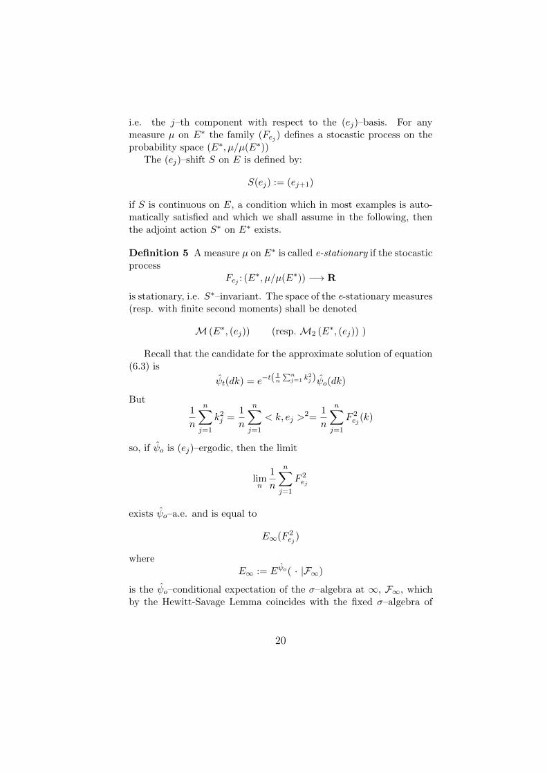
i.e. the j–th component with respect to the (ej)–basis. For anymeasure µ on E∗ the family (Fej ) defines a stocastic process on theprobability space (E∗, µ/µ(E∗))

The (ej)–shift S on E is defined by:

S(ej) := (ej+1)

if S is continuous on E, a condition which in most examples is auto-matically satisfied and which we shall assume in the following, thenthe adjoint action S∗ on E∗ exists.

Definition 5 A measure µ on E∗ is called e-stationary if the stocasticprocess

Fej : (E∗, µ/µ(E∗)) −→ R

is stationary, i.e. S∗–invariant. The space of the e-stationary measures(resp. with finite second moments) shall be denoted

M (E∗, (ej)) (resp.M2 (E∗, (ej)) )

Recall that the candidate for the approximate solution of equation(6.3) is

ψt(dk) = e−t(1n

∑nj=1 k

2j )ψo(dk)

But1

n

n∑j=1

k2j =

1

n

n∑j=1

< k, ej >2=

1

n

n∑j=1

F 2ej (k)

so, if ψo is (ej)–ergodic, then the limit

limn

1

n

n∑j=1

F 2ej

exists ψo–a.e. and is equal to

E∞(F 2ej )

whereE∞ := Eψo( · |F∞)

is the ψo–conditional expectation of the σ–algebra at ∞, F∞, whichby the Hewitt-Savage Lemma coincides with the fixed σ–algebra of

20

the adjoint action S∗, on (E∗, ψo), of the (ej)–shift. the (ej)–shift Son E, defined by:

S(ej) := (ej+1)

(to be sure of the existence of this adjoint action, one has to assumethat S is continuous on E, a condition which, in most examples, isautomatically satisfied). In conclusion [AcRoSmo], [Ro]:

Theorem 3 For an (ej)-stationary initial measure ψo, the limit of the

approximate solutions exists ψo–a.e.. If ψo has finite second moments,the limit is finite ψo–a.e..

One can prove [AcOb2] that there exists a function

k ∈ E∗ −→ ||k|| ∈ (0,+∞)

(the norm on H is denoted | · |) such that for any ψo ∈M2 (E∗, (ej))

||k||2 = Eψo∞ (F 2ej )(k) = lim

n

1

n

n∑j=1

< k, ej >2 , ψo − ∀k

From the explicit form, it follows that k → ||k||2 is a quadratic formwhose associated bilinear symmetric form can be written

(h|k) = limn

1

n

n∑j=1

< h, ej >< ej , k >

where < ·, · > denotes the scalar product in H which is compatiblewith the duality < E∗, E >. Notice that, by Parseval identity, thescalar product (· | ·) is identically zero on the Hilbert space H.

Theorem 4 The Levy-laplacian in momentum space is the linearoperator ∆L , from M2 (E∗, (ej)) to M (E∗, (ej)), defined by:

∆L = limn

1

n

n∑j=1

p2j ; (pjψo)(dk) =< k, ej > ψo(dk)

The associated heat semigroup is

P tψo(dk) = et∆Lψo(dk) = e−tEψo∞ (F 2

e1)ψo(dk) (33)

21

Remark The semigroup P t is Markovian in the sense that (i) posi-tive measures are mapped into positive measures and (ii) the identity(for the convolution among measures) is mapped into the identity

P tδo = δo

where δo denotes the atomic probability measure at 0.

As a corollary of this result, we obtain the eigenvalues and eigen-vectors of the Levy laplacian on M (E∗, (ej)).

Theorem 5 A measure ψo is an eigenvector of ∆L if and only if it isergodic. In this case the corresponding eigenvalue is minus the meanvalue of F 2

e1 (second moment of Fe1)

Eψo(F 2e1) =

∫E∗

F 2e1(k)ψo(dk) =

∫E∗

< k, e1 >2 ψo(dk)

Proof

P tψo(dk) = e−t||k||2ψo(dk) = et∆Lψo(dk) =

= e−t 1

nlimn

∑nj=1 F

2ej

(k)ψo(dk) = e−tE

ψo (F 2e1

)ψo(dk)

Differentiating in t one gets the resultRemark The above result shows that Spec(∆L) =⊇ (−∞, 0). In

fact one can show that on M (E∗, (ej)), Spec(∆L) = (−∞, 0]. Thisfollows froom the explicit formula (8.1) and from the fact that P t

decreases the variation norm.Remark The spectrum is highly degenerate: if ψ,ϕ are eigenvec-

tors corresponding respectively to the eigvalues λ1 , λ2 then, by thederivation property of ∆L

∆L(ψϕ) = (∆Lψ)ϕ+ ψ(∆Lϕ) = (λ1 + λ2)ψϕ

Thus the sufficiently smooth eigenvectors are an algebra graded by thesemigroup [0,∞).

Remark Connection with the Obata-Hida results on eigenvalues.Remark Since the Levy–heat semigroup in momentum space is

given by the explicit formula (8.1), it can obviously be analyticallycontinued to the right half–plane Re(z) ≥ 0 and its boundary valueon the imaginary axis is invertible and satisfies the Levy-Schrodinger

22

equation. Since to any given (classical) Markov semigroup on a com-

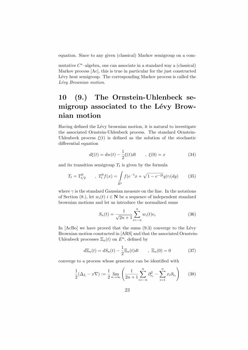
mutative C∗–algebra, one can associate in a standard way a (classical)Markov process [Ac], this is true in particular for the just constructedLevy heat semigroup. The corresponding Markov process is called theLevy Brownian motion.

10 (9.) The Ornstein-Uhlenbeck se-

migroup associated to the Levy Brow-

nian motion

Having defined the Levy brownian motion, it is natural to investigatethe associated Ornstein-Uhlenbeck process. The standard Ornstein-Uhlenbeck process ξ(t) is defined as the solution of the stochasticdifferential equation

dξ(t) = dw(t)− 1

2ξ(t)dt , ξ(0) = x (34)

and its transition semigroup Tt is given by the formula

Tt = T 0t/2 , T 0

t f(x) =

∫R1

f(e−tx+√

1− e−2ty)γ(dy) (35)

where γ is the standard Gaussian measure on the line. In the notationsof Section (8.), let wi(t) i ∈ N be a sequence of independent standardbrownian motions and let us introduce the normalized sums

Sn(t) =1√

2n+ 1

n∑i=−n

wi(t)ei (36)

In [AcBo] we have proved that the sums (9.3) converge to the LevyBrownian motion constucted in [ARS] and that the associated Ornstein-Uhlenbeck processes Ξn(t) on En, defined by

dΞn(t) = dSn(t)− 1

2Ξn(t)dt , Ξn(0) = 0 (37)

converge to a process whose generator can be identified with

1

2(∆L − x∇) :=

1

2limn→∞

(1

2n+ 1

n∑i=−n

∂2ei −

n∑i=1

xi∂ei

)(38)

23

this is the Levy Ornstein–Uhlenbeck process. More precisely: Theorem

1. (i) For any fixed t ≥ 0 the operators T(n)t and P

(n)t converge stron-

gly, i.e. pointwise in sup norm on F , to bounded operators Tt and Ptrespectively. The families Ttt≥0 and Ptt≥0 are strongly continuousMarkov semigroups on F , hence on C.

(ii) The semigroups Tt and Pt give rise to two Markov processesΞ(t) and W (t) with state space S. Moreover, these processes are re-spectively the limits in distribution of the finite-dimensional processesΞn(t) and Sn(t).

(iii) The law Λ1 of W (1) is an invariant probability of the processΞ(t).

(iv) The process with initial distribution Λ1 is symmetric.

11 (10.) The Cesaro algebra

The results in the following sections have been obtained in collabora-tion with N.Obata [AcOba2]. In the following, if (an) is a sequence ofreal or complex numbers, we define

κN ((an)) :=1

N

N∑j=1

aj

if the limit

limN→∞1

N

N∑n=1

an = limN→∞κN ((an)) =: κo((an))

exists, it is called the Cesaro mean of (an). Let `(c)(N) denote the

space of sequences (an) of complex numbers such that

limsup1

n

n∑j=1

|an|ν < +∞ ; ∀ν ∈ N (39)

Clearly `(c)(N) contains `∞(N) and, by Holder’s inequality, `(c)(N) isa ∗−algebra, called, in the following, the Cesaro algebra. The Cesaromean κo is defined on a linear subspace of `(c)(N). The functionp : `(c)(N) → R+ defined by

p(h)2: = limsupn1

n

n∑j=1

< h, ej >2

24

is a seminorm on `(c)(N) (in particular it is everywhere finite on`(c)(N)). The Cesaro mean is continous for this seminorm in the sensethat, if the sequence (an) admits a Cesaro mean then, denoting 1 theconstant sequence equal to 1, one has

|κN ((an))| = |κN (1 · (an))| ≤ κN (1)1/2κN (|(an)|2)1/2 = κN ((|a2n|))1/2

which implies

limsupN |κN ((an))| = |κo((an))| ≤ p((an))

So the restriction of the Cesaro mean on its natural domain is conti-nuous for the p-seminorm.

Theorem 6 The Cesaro mean κo has a positive Hahn-Banach ex-tension κ to all of `(c)(N) continuous with respect to the seminormp.

Proof This follows from the Hahn–Banach theorem for positivefunctionals (cf. [Schaffer ] pg.76 and 86). In the following E ⊆ H ⊆ E∗

shall denote a standard triple [Hid].

Lemma 1 Suppose that µ ∈ M(E∗, e) has moments of any order.Then the set of k ∈ E∗ such that for every ν ∈ N the limit

limn1

n

n∑j=1

< k, ej >ν (40)

exists finite, has µ−measure one. Moreover, the set E∗e of all k ∈ E∗such that

limsupn1

n

n∑j=1

| < k, ej > |ν < +∞ ; ∀ν ∈ N (41)

is a measurable linear subspace of E∗ which has µ-measure 1 for anyµ ∈M(E∗, e) with moments of all orders. As a consequence of Lemma

(10.2) above, there exists a pre-scalar product, denoted (·|·)o, on E∗ewith the following property: for any pair of vectors h, k ∈ E∗e suchthat the limit

limn1

n

n∑j=1

< h, ej >< k, ej > (42)

exists, this limit is equal to (h|k)o.

25

Definition 6 Denote η = ηe the quotient map from E∗e to its quotientE∗e/(·|·)o, by the elements of zero (·|·)o − norm; He the completion ofE∗e/(·|·)o for the induced scalar product and (· | ·) the scalar productHe. The space He shall be called the Cesaro Hilbert space of the pairE∗, e = (ej).

12 (11.) Algebras of operator valued

measures

The space M(E∗) of bounded signed measures on E∗. is an abe-lian algebra under convolution. The Fourier transform establishes anisomorphism of M(E∗) with a closed subalgebra B(E), of Cb(E)–thecontinuous bounded functions on E with pointwise multiplication andsup norm – called the Fourier-Stiltjes algebra of E. By the infinitedimensional version of Bochner’s theorem, the elements of B(E) areprecisely the continuous positive definite functions on E. Let

M :=M∞(E∗, e) (43)

denote the family of all measures µ ∈ M(E∗, e) with finite momentsof all orders. M is a closed subalgebra ofM(E∗) and its image underFourier transform shall be denoted B. The structure of C∗–algebra onCb(E) is induced on B and transported toM by Fourier transform. Bythe infinite dimensional version of Bochner’s theorem, the elements ofB(E) are precisely the continuous positive definite functions on E.

SinceM, defined by (11.0) is abelian, if H is a Hilbert space, thenthere is a unique C∗-cross norm on the algebraic tensor productM⊗(o)

B(H) [Sak] and we denoteM⊗B(H) the closure of this algebraic tensorproduct by this norm.

A B(H)-valued measure on E∗ is a map

ν:A ⊆ E∗ −→ ν(A) ∈ B(H)

from measurable subsets of E∗ to B(H) such that, for any normalstate ϕ on B(H), the map A 7→ ϕ(ν(A)) is countably additive. Ifν ∈ M(E∗) and F :E∗ → B(H) is a strongly continuous uniformlybounded function, then the map

A ⊆ E∗ 7→∫AF (k)ν(dk)

26

where the integral is meant in the ultraweak topology, is an exampleof B(H)-valued measure. We use the map

ν ⊗ b ∈M⊗(o) B(H) 7→ ν(·)b (44)

to identify any M⊗B(H)-valued function of the form

k ∈ E∗ 7→ ν ⊗ F (k)

(ν ∈ M(E∗), F - a B(H)−valued, strongly continuous, boundedfunction) to the B(H)-valued measure

A ⊆ E∗ 7→∫AF (k)ν(dk) (45)

moreover we shall often use equivalently the notations

F (k)ν(dk) ; ν ⊗ F (·) (46)

to mean the measure (11.2).Let Γ ≡ Γ(L2(R+)⊗He) denote the Fock space over L2(R+)⊗He ≡

L2(R+;He) ; W (F ) (F ∈ L2(R+;He)) the Weyl operators on Γ; Φ thevacuum vector in Γ. We recall that for each t ∈ R+, Γ is canonicallyisomorphic to

Γ(L2([o, t];He))⊗ Γ(L2([t,+∞);He))

and in this isomorphism the Fock vacuum Φ is identified to the tensorproduct of the corresponding Fock vacua, denoted Φt]⊗Φ[t. We shalluse the notations

Γt]: = Γ(L2(o, t]⊗He)⊗Φ[t ; Γ[t: = Φt]⊗Γ(L2(t2 +∞]⊗He) (47)

more generally, for an interval [a, b] ⊆ R, we write

Γ[a,b] := Φa] ⊗ Γ(L2(a, b)⊗He)⊗ Φ[b (48)

Finally St shall denote the time shift in L2(R+;He), St: = Γ(St) itssecond quantization acting on Γ(L2(R+;He)) and

uot : = Ad St = St(·)S∗t (49)

the time-shift endomorphism on B(Γ(L2(R+, He))).

27

Definition 7 Let A be ∗-algebra and (uot ) a 1-parameter endomor-phism group of A such that any uot has a left inverse denoted uo−t.

Let, for each t ≥ 0, be given a sub-algebra D(t) ⊆ A and a mapjt:D(t) −→ A. The family jt, D(t) (t ≥ o) is called an (uot ) −cocycle if for any s, t ≥ o:

js uos jt uo−s = js+t (50)

the equality being meant on D(t + s) and in the sense that, on thisdomain, both sides are well defined and the identity holds.

If moreover the algebra A admits a past and a future filtrationbased on R+, denoted respectively (At]), (At]) and each jt (t ≥ 0)satisfies the conditions

jt(at b[t) = jt(at)b[t ; ∀at ∈ D(t) ; ∀b[t ∈ D(t) ∩ A[t (51)

jt(D(t) ∩ At]) ⊆ At] (52)

then the family jt, D(t) is called a Markovian cocycle.

Lemma 2 In the notations of Definition (10.3) the 1-parameter fa-mily of maps

jt:M(E∗) −→M(E∗)⊗ B(Γt]) ⊆M(E∗)⊗ B(Γ)

defined by

jt(ν): = ν ⊗W (χ[o,t] ⊗ η(·)) = W (χ[o,t] ⊗ η(k))ν(dk) (53)

and extended to M(E∗)⊗ B(Γ[t) by

jt(ν ⊗ b[t): = jt(ν)b[t ; b[t ∈ B(Γ[t) (54)

is a Markovian cocycle.

By the quantum Feynman-Kac formula [Ac] the Markovian cocycle(jt) defines a Markovian semigroup on M.

Lemma 3 The Markovian semigroup on M, defined by the Marko-vian cocycle (jt) has the form:

(P tν)(dk) = e−t2||η(k)||2ν(dk) (55)

In particular, the extension of P t on M2(E∗, e) coincides with theLevy heat semigroup in momentum space.

28

13 (12.) Identification of the Levy Bro-

wnian motion

In the notations of the previous Section, recall that the Fourier tran-sform defines a continuous ∗-isomorphism of M onto the subalgebraof Cb(E), denoted B whose elements are the Fourier transforms of thee-stationary bounded measures on E∗. Using this isomorphism weidentify M with B moreover we define

(F ⊗ ıB) jt (F−1 ⊗ ıB) = : jt :B → B ⊗ B(Γ) (56)

where ıB is the identity map on B(Γ), and

F P t F−1 =: P t : B → B (57)

DenotingA: = B ⊗ B(Γ) (58)

ϕo, the state on B(Γ) defined by the vacuum vector, i.e.

ϕo(b) =< Φ, bΦ > ; b ∈ B(Γ) (59)

and mo an arbitrary state on B, we obtain

Theorem 7 The classical algebraic stochastic process A, ϕ: = mo⊗ϕo, (jt) with state algebra B is a classical stochastic process stochasti-cally isomorphic to the Levy Brownian motion constructed in Section(8.) with initial state mo.

References

[Ac] Accardi L.: On the quantum Feynmann-Kac formula. Rendi-conti del seminario Matematico e Fisico, Milano 48(1978) 135-180.

[AcGi] Accardi L., Gibilisco P.: The Schrodinger representation onHilbert bundles. in: Probabilistic Methods in Mathematical Physics,eds. F.Guerra, M.Loffredo, World Scientific 1993

[AcGiVo] L. Accardi P. Gibilisco, I.V. Volovich; The Levy laplacianand the Yang-Mills equations. Rendiconti dell’Accademia dei Lincei,1993

[AcGiVo2] L. Accardi P. Gibilisco, I.V. Volovich; Yang–Mills gaugefields as harmonic functions for the Levy Laplacian, Russian Journalof Mathematical Physics (1994)

29

[AcSmo1] L. ACCARDI, D. SMOLYANOV, On laplacians and tra-ces, Rendiconti Seminario Matematico, Bari, Ottobre 1993, PreprintVolterra.

[AcSmo2] Luigi Accardi, Paolo Roselli, Oleg G. Smolyanov TheBrownian Motion Generated by the Levy-Laplacian MatematicheskieZametki, 54 (1993) 144–148

[AcBo] L. Accardi, V. I. Bogachev, The Ornstein-Uhlenbeck pro-cess and the Dirichlet Form Associated to the Levy laplacian VolterraPreprint, September (1994)

[AcOba1] Luigi Accardi, Nobuaki Obata, Derivation property ofthe Levy laplacian in: White noise analysis and quantum probability,N.Obata (ed.), RIMS Kokyuroku 874, Publications of the ResearchInstitute for Mathematical Sciences, Kyoto (1994) 8–19

[AcOba2] Luigi Accardi, Nobuaki Obata, On the Fock space reali-zation of the Levy Brownian motion, Volterra Preprint (1994)

[Arv] Arvesom W.B., Analyticity in operator algebras, Am. J.Math. 89(1967)578

[AHDM] Atiyah M.F., V.G.Drinfeld. N.J.Hitchin, Yu.I.Manin:Construction of instantons, Phys. Lett. 65 A (1978) 425–461

[Driv1] Driver B., Loop space, curvature and quasi-invariance,Volterra Preprint N.123, October 1992.

[Driv2] Driver B., JFA. 83 (1989) 185-231 Driver B.K., Classifi-cations of bundle connection pairs by parallel translation and lassos,J.Func. Anal. 83 (1989) 185 231.

[FuKa] Fuglede B., Kadison R.V., Determinant theory in finitefactors, Ann. of Math. 55(1952) 520–530

[FuLu] Fuchsteiner B., W.Luxemburg (eds.) Geometry and analy-sis, volume dedicated to D.Langwitz. Birkhauser (1992)

[Hida1] Hida T., Analysis of Brownian functional Carleton Mathe-matics Lecture Notes, vol.13, 1975; 2nd ed., 1978

[Hida2] Hida T., The impact of classical functional analysis onwhite noise calculus, Preprint Centro V.Volterra, n.90, (1992) Rome

[Ros] Paolo Roselli, Laplaciani in spazi a infinite dimensioni eapplicazioni. Tesi, Universita di Roma La Sapienza, (1992)

[Sak] Sakai S.: C∗-algebras and W ∗-algebras. Ergebr.d.math. 60Springer Verlag Berlin 1971.

[Scha] H.H.Schaefer, Banach lattices and positive operators, Springer-Verlag, (1974).

30