arX

iv:h

ep-t

h/98

0805

3v1

10

Aug

199

8

hep-th/9808053 ITP–UH–15/98

String-induced Yang-Mills coupling to self-dual gravity ∗

Chandrashekar Devchand

Max-Planck-Institut fur Mathematik in den Naturwissenschaften

Inselstraße 22-26, 04103 Leipzig, Germany

E-mail: devchand@mis.mpg.de

Olaf Lechtenfeld

Institut fur Theoretische Physik, Universitat Hannover

Appelstraße 2, 30167 Hannover, Germany

http://www.itp.uni-hannover.de/˜lechtenf/

Abstract

By considering N=2 string amplitudes we determine the (2+2)-dimensional target

space action for the physical degrees of freedom: self-dual gravity and self-dual Yang-

Mills, together with their respective infinite towers of higher-spin inequivalent picture

states. Novel ‘stringy’ couplings amongst these fields are essential ingredients of an

action principle for the effective target space field theory. We discuss the covariant

description of this theory in terms of self-dual fields on a hyperspace parametrised

by the target space coordinate and a commuting chiral spinor.

∗ supported in part by the Deutsche Forschungsgemeinschaft; grant LE-838/5-2

1 Introduction

We have recently presented a covariant description of the physical degrees of freedom of the

N=2 open string in terms of a self-dual Yang-Mills theory on a hyperspace parametrised by the

coordinates of the (2+2)-dimensional target space x±.α together with a commuting chiral spinor

η± [1]. The infinite tower of massless string degrees of freedom, corresponding to the inequiva-

lent pictures (spinor ghost vacua) of this string [2], are compactly represented by a hyperspace

generalisation of the prepotential originally used by Leznov [3, 4] to encode the dynamical de-

gree of freedom of a self-dual Yang-Mills (SDYM) theory. The generalised hyperspace Leznov

Lagrangean yields an action describing the tree-level N=2 open string amplitudes [1]. This

description reveals the symmetry algebra of the space of physical states to be the Lie-algebra

extension of the Poincare algebra [5] obtained from the N=1 super-Poincare algebra by chang-

ing the statistics of the Grassmann-odd (fermionic) generators. Picture-raising [6, 7] is thus

interpreted as an even variant of a supersymmetry transformation.

The purpose of this paper is to investigate whether closed strings allow incorporation into

the above picture. The physical centre-of-mass mode is well-known to describe self-dual gravity

(SDG) in (2 + 2) dimensions [8]. The effect of inequivalent picture states has, however, hitherto

not been taken into account. As for the open case, the closed sector physical state space

consists of an infinite tower of massless picture-states of increasing spin [9, 10]. In particular the

scattering of open strings with closed strings determines a particular coupling of the SDG tower

of picture states with the SDYM tower [11]. Motivated by our previous results for the open

string sector [1], we first (in section 2) set up the general framework of curved-hyperspace self-

duality, in the expectation that it underlies the full (open + closed) N=2 string dynamics. This

involves a generalisation of the formalism previously developed to study self-dual gravity [12]

and self-dual supergravity [13] to the hyperspace introduced in [1]. Our formalism is basically

a field-theoretical variant of the twistor construction. The dynamical degrees of freedom of

hyperspace self-duality are seen to be encoded in a hyperspace variant of Plebanski’s ‘heavenly’

equation [14].

Gauge covariantising the construction yields a curved hyperspace variant of the Leznov

equation as well. These two equations, however, do not provide a complete description of the

effective N=2 string dynamics, for perusal of string scattering amplitudes (section 3) reveals

further couplings between the gravitational and gauge degrees of freedom. Taking these into

account yields an effective target space action (section 4) for the two infinite towers of target

space fields. We discuss the hyperspace-covariant description of this action and write down

homogeneous hyperspace equations of motion. Finally, a consistent truncation is performed

(section 5) to multiplets of 9 fields from the Plebanski tower and 5 from the Leznov tower.

Their combined action is rather reminiscent of the maximally helicity-violating projection of

(non-self-dual) light-cone N=8 supergravity plus N=4 super Yang-Mills, with the replacement

of the fermionic chiral superspace coordinate by a commuting spinor.

1

2 Self-dual gravity picture album

Consider a self-dual chiral hyperspace M+ with coordinates {xα.

µ, ηα}, where ηα is a commuting

spinor and xα.

µ are standard coordinates on R2,2. As for self-dual superspaces, only half the

global tangent space group SO(2, 2) ≃ SL(2, R)× SL(2, R) is gauged. One of the world indices

is therefore identical to the corresponding tangent index (denoted by early Greek indices α, β, γ,

etc.) and only the dotted index has ‘world’ and ‘tangent’ variants. The components of the

spinor ηα therefore do not transform under space diffeomorphisms. Covariant derivatives in the

chiral hyperspace therefore take the form

Dα = ∂α + Eβ.

µα ∂

β.

µ+ ωα , D

α.

α= Eβ

.

µ

α.

α∂

β.

µ+ ω

α.

α, (2.1)

with the partial derivatives ∂α ≡ ∂∂ηα and ∂

α.

µ≡ ∂

∂xα.

µ. The components of the spin connection

(ωα, ωα.

α) are determined in terms of the vielbein fields in virtue of zero-torsion conditions. We

choose them in a self-dual gauge, ωα = (ωα).

γ.

βΓ.

β.

γand ω

α.

α= (ω

α.

α).

γ.

βΓ.

β.

γ, i.e. taking values in

the Lie algebra of the gauged SL(2, R). They therefore act on dotted tangent space indices.

Thus restricting the local part of the tangent space group to half of the Lorentz group is (gauge)

equivalent to imposing self-duality on the corresponding curvatures, viz.,

[Dα,Dβ] = ǫαβR

[Dα,Dβ.

β] = ǫαβR.

β

[Dα.

α,D

β.

β] = ǫαβR

.

α.

β.

(2.2)

With the undotted indices thus ‘de-gauged’, we can proceed in analogy to the Yang-Mills case

[1] and enlarge M+ to a harmonic space with coordinates {x±.µ, η±, u±α }, where x±.µ = u±

α xα.

µ,

and η± = u±α ηα.

The equations (2.2) are equivalent to the following curvature constraints:

[D+,D+.

β] = 0 , [D+

.

α,D+

.

β] = 0 (2.3)

[D−,D−.

β] = 0 , [D−

.

α,D−

.

β] = 0 (2.4)

[D+,D−] = R , [D+,D−.

β] = [D+

.

β,D−] = R.

β, [D+

.

α,D−

.

β] = R

.

α.

β. (2.5)

These allow, by the usual Frobenius argument, the choice of an analytic Frobenius frame in

which D+,D+.

βare flat. In this frame, diffeomorphism and Lorentz invariances are determined

in terms of analytic (independent of x+.

µ, η+) degrees of freedom. We do not transform the

harmonic variables u±α . This facilitates the application to N=2 string theory, which requires a

fixing of the complex structure and the use of corresponding light-cone variables. Moreover, let

us choose the transformation parameters to be independent of the spinorial variables η±. We

thus consider the following action of the local group of infinitesimal diffeomorphisms

δ x+.

µ = λ+.

µ(x+.

µ, u±) , δ x−.µ = λ−.µ(x+.

µ, x−.µ, u±) , δ η± = 0 . (2.6)

2

The gauge choice D+ = ∂+ and D+.

β= ∂+

.

βis tantamount to the following relationship between

the non-analytic parameter λ−.µ and the analytic parameter of local sl(2, R) transformations

λ.

β.

α= λ

.

β.

α(x+

.

µ, u±):

∂+.

αλ−.µ = −λ

.

µ.

α. (2.7)

In this frame the covariant derivatives take the form

D+ = ∂+

D+.

α= ∂+

.

α

D− = −∂− + E.

µ∂−.

µ+ E−−.µ∂+

.

µ+ ω−

D−.

α= −E

.

µ.

α∂−.

µ+ E−−.µ

.

α∂+.

µ+ ω−

.

α,

(2.8)

where the vielbein fields transform as:

δ E.

µ = E.

ν∂−.

νλ+

.

µ

δ E−−.µ = D−λ−.µ

δ E.

µ.

α= D−

.

αλ+

.

µ + λ.

β.

αE.

µ.

β

δ E−−.µ.

α= D−

.

αλ−.µ + λ

.

β.

αE−−.µ.

β.

(2.9)

We note that the fields E.

µ and E.

µ.

αhave transformations depending only on analytic transfor-

mation parameters. Moreover, in virtue of (2.4) and (2.5) these fields are analytic, satisfying

the set of equations

∂+E.

µ = 0 = ∂+.

αE.

µ

∂+E.

µ.

β= 0 = ∂+

.

αE.

µ.

β

D−E.

µ.

α+ D−

.

αE.

µ = 0

D−[.

βE.

µ.

γ]= 0 .

(2.10)

We may therefore choose x+.

µ such that E.

µ = 0 and E.

µ.

α= δ

.

µ.

α. In this gauge, the relation (2.7)

is supplemented by

∂−.

αλ+

.

µ = λ.

µ.

α. (2.11)

All diffeomorphisms are thus effected by residual Lorentz transformations, allowing world indices

to be freely replaced by tangent indices with an action of the Lorentz group. In this gauge, the

last two equations in (2.10) yield the conditions

(ω−).

δ.

γ= 0 , (ω−

[.

β).

δ.

γ]= 0 . (2.12)

The former condition is consistent with the η-independence of the Lorentz parameters λ.

β.

α.

Clearly, the curvature constraints R = 0 = R.

αfollow. The non-trivial covariant derivatives

3

therefore take the simpler form

D− = −∂− + E−−.µ∂+.

µ

D−.

α= −∂−

.

α+ E−−.µ

.

α∂+.

µ+ ω−

.

α.

(2.13)

For the vielbeins appearing here, the torsion constraints implicit in (2.4) and (2.5) yield the

equations,

∂+E−−.µ = 0 = ∂+.

αE−−.µ (2.14)

∂+E−−.µ.

β= 0 (2.15)

∂+.

αE−−.γ.

β= (ω−

.

β).

γ.

α. (2.16)

The latter, together with (2.12) and the tracelessness of sl(2, R) matrices (viz. (ω−.

β).

α.

α= 0), yield

an expression for the connection component ω−.

αand vielbein E−−.µ

.

α,

(ω−.

α

).γ.

β= ∂+

.

αE−−.γ.

β= ∂+

.

α∂+

.

γ∂+.

βF−−−− , (2.17)

where the prepotential F−−−− is η−-independent, ∂+F−−−− = 0 , so as to satisfy (2.15). The

η+-dependence of E−−.µ.

αyields the remaining vielbein, which satisfies the linear equation

D−.

αE−−

.

β = − ∂−E−−.

β.

α. (2.18)

The torsion constraint from (2.4),

D−[.

βE−−.µ.

γ]= 0 , (2.19)

yields, on using an analytic pre-gauge invariance of F−−−−, the extended Plebanski equation,

∂−.α∂+.

αF−−−− = 1

2 ∂+.

α∂+.

βF−−−− ∂+.

α∂+.

βF−−−− . (2.20)

Since F−−−− is η−-independent and transforms in an η-independent fashion, it can be thought

of as a Laurent expansion in η+. This equation therefore encapsulates an infinite tower of

equations. Its Lagrangean is of the compact Plebanski form, with a potential term of the cubic

Monge-Ampere type:

L(−8)P = 1

2 ∂−.αF−−−− ∂+.

αF−−−− + 1

6 F−−−− ∂+.

α∂+.

βF−−−− ∂+.

α∂+.

βF−−−− . (2.21)

So far we have just considered pure self-dual gravity in (2+2)-dimensional chiral hyperspace.

Let us now add self-dual Yang-Mills degrees of freedom by gauge covariantising the curvature

constraints (2.5). In the analytic gauge (A+ = 0 = A+.

α), this is achieved by ‘minimally coupling’

Yang-Mills potentials to the negatively charged covariant derivatives, with coupling constant g,

D− → D− = D− + gA−

D−.

α→ D−

.

α= D−

.

α+ gA−

.

α.

(2.22)

4

The components of the gauge potentials take values in the Lie algebra of the gauge group and

have the gauge transformations

A− → ΛA− Λ−1 − 1g D−ΛΛ−1

A−.

α→ ΛA−

.

αΛ−1 − 1

g D−.

αΛΛ−1 ,

(2.23)

with analytic parameter Λ = Λ(x+, η+, u) taking values in the gauge group.

The coupled gravity-Yang-Mills self-duality conditions thus take the form of the curvature

constraints

[D−.

α, D−

.

β] = 0 (2.24)

[D−, D−.

α] = 0 (2.25)

[∂+, D−] = F , [∂+, D−.

α] = [∂+

.

α, D−] = F.

α(2.26)

[D+.

α, D−

.

β] = R

.

α.

β+ F

.

α.

β. (2.27)

Here, F.

α.

β(x, η), resp. R

.

α.

β(x, η), are symmetric and have the corresponding R

2,2 Yang-Mills,

resp. Weyl, self-dual curvatures as their evaluations at η = 0. The fields F , F.

αand F

.

α.

βtake

values in the gauge algebra.

In virtue of (2.26) and (2.27) we have the expressions

A− = ∂+Φ−− , A−.

α= ∂+

.

αΦ−− (2.28)

F = ∂+∂+Φ−− , F.

α= ∂+∂+

.

αΦ−− , F

.

α.

β= ∂+

.

β∂+.

αΦ−− (2.29)

in terms of a generalised Leznov prepotential Φ−−. These expressions maintain their flat space

forms [1] since in the analytic gauge the positively-charged derivatives remain ‘flat’ in both

gauge and gravitational senses. The Plebanski prepotential F−−−− is a scalar under the gauge

group; its equation remains unmodified by the Yang-Mills coupling. This is consistent with the

stress-free self-dual Yang-Mills field not providing any source for the gravitational field. The

equation for Φ−−, on the other hand, is a generally covariant version of the Leznov equation

obtained from the gauge-algebra valued part of (2.24),

D−.α∂+.

αΦ−− + g

2

[∂+

.

αΦ−− , ∂+.

αΦ−−

]= 0 . (2.30)

More explicitly,

∂−.α∂+.

αΦ−− = ∂+

.

α∂+.

βF−−−− ∂+.

α∂+.

βΦ−− + g

2

[∂+

.

αΦ−− , ∂+.

αΦ−−

]. (2.31)

This is the equation which determines the effective dynamics on R2,2 of the residual vector

potential A−.

α= ∂+

.

αΦ−−. The remaining equation for Φ−−, the one arising from the gauge-

algebra part of (2.25), determines the η+-evolution of A−.

αfrom its η+ = 0 ‘initial data’, namely,

∂−A−.

α= ∂−

.

α∂+Φ−− + E−−

.

β ∂+.

α∂+.

βΦ−− − E−−

.

β.

α∂+∂+

.

βΦ−− + g

[∂+Φ−− , ∂+

.

αΦ−−

]. (2.32)

5

It may be noted that the combined system of equations (2.20) and (2.31) cannot be derived from

an action principle, since their mutual coupling appears only in (2.31). In the next section, we

shall see that new string-induced couplings provide a remedy.

The hyperspace fields F−−−−(x, η) and Φ−−(x, η) can clearly be thought of as R2,2 fields,

taking values in the infinite-dimensional algebra spanned by polynomials of ηα. Such algebras

have been investigated in [15]. In particular, consistent higher-spin free-field equations were

shown to arise as components of zero-curvature conditions for connections taking values in such

algebras. It remains to be seen whether our equations allow interpretation as interacting variants

of these free-field equations.

3 Open and closed string amplitudes

Having obtained the dynamical equations (2.20) and (2.31) for the self-dual hyperspace grav-

itational and gauge degrees of freedom, we are ready to ask whether these provide a correct

description of N=2 string dynamics. By considering scattering amplitudes, we shall see that

these naive equations require modification which, moreover, yields equations derivable from an

action principle. The required modification includes ‘stringy’ contributions which vanish in the

infinite string tension limit.

Since we would like to describe in particular the coupling of self-dual Yang-Mills to self-dual

gravity (in 2+2 dimensions), let us consider a general (mixed) scattering amplitude involving nc

closed and no open N=2 strings. Each such amplitude has a topological expansion in powers

of the open string coupling g and in powers of a phase given by the angle θ of the spectral

flow. The expansion is governed by the world-sheet instanton number c ∈ Z and the world-sheet

Euler number χ = 2 − 2h − b − x in the presence of h handles, b boundaries and x cross-caps.

Introducing the ‘spin’

J = 2nc + no − 2χ = 2nc + no − 4 + 4h + 2b + 2x (3.1)

one finds [16, 2, 1] for any given choice of (nc, no), the amplitude,

A =∑

J

gJ AJ =∑

J,c

(2J

J+c

)gJ sinJ−c θ

2 cosJ+c θ2 AJ,c (3.2)

where AJ,c is a correlator of vertex operators V on a world-sheet of fixed topology, integrated

over all moduli. Clearly, J runs upwards in steps of two, starting from Jmin = 2nc+no−2−2δno,0.

Due to unbalanced spinor ghost zero modes, the instanton sum is constrained to |c| ≤ J . In four

dimensions, the open-string coupling g is just the (dimensionless) Yang-Mills gauge coupling,

while the closed-string coupling g2 is related to the (dimensionful) gravitational coupling κ via

κ ∼√

α′g2 (3.3)

where α′ denotes the inverse string tension.

6

The string coupling g and the θ angle change under global SO(2, 2) tangent space transfor-

mations of the target space [4, 9, 1]. We may therefore set g = 1 and θ = 0 for convenience.1

As a consequence, only the top instanton number, c = J , contributes, i.e.

A =∑

J

AJ,J (3.4)

with AJ,J carrying helicity J .2 Each partial amplitude AJ,J contains an integral over four moduli

spaces Mi , corresponding to the world-sheet supergravitational non-gauge degrees of freedom

of the metric, the two gravitini, and the Maxwell field. The respective real dimensions are

dimRMmetric = 2nc + no − 3χ = J − χ

dimRM±gravitino = 2nc + no − 2χ ± c = J ± c

c=J−→{

2J (+)

0 (−)(3.5)

dimRM±Maxwell = 2nc + no − χ = J + χ

The gravitini modular integral can be performed and yields 2J picture-raising insertions P+ in

the path integral [7, 10]. For χ > 0, the Maxwell modular integral is trivial due to spectral flow

invariance. Likewise, the metric moduli for positive χ reduce to the world-sheet positions of

the vertex operators. The final matter-plus-ghost path integral is a superconformal correlation

function of antighost zero modes, picture-raisers, and (canonical) local vertex operators which

create the string states from the vacuum.

Which string states are to be scattered? It is known from the relative BRST cohomology of

the open N=2 string that its spectrum consists of a single massless physical state at each value of

the picture charge (π+, π−) labelling inequivalent spinor ghost vacua [17]. An internal symmetry

group G is incorporated by requiring these states to carry Chan-Paton adjoint representation

indices of G. The difference π+−π− changes continuously under the action of spectral flow.

Since the Maxwell modular integration entails an averaging over the parameter ρ of spectral

flow, one must identify the equivalent sectors (π+, π−) ∼ (π++ρ, π−−ρ). We shall use the

π+=π− representative. The total picture number π ≡ π++π− takes integral values, and the

helicity of the state is j = 1+π/2 ∈ 12Z. For states of non-zero momentum k, picture-changing

can be used to implement an equivalence relation among all pictures [17]. In this case, a single

open string state interacts with itself, unless the Chan-Paton group G is abelian. Such an

identification, however, ruins target space covariance, because picture-raising by P+ increases

not only π by one, but also the helicity j by half a unit. It is therefore advantageous to

distinguish the unique physical states in different pictures π. The canonical (j=0) open string

state resides at π= − 2. The corresponding (canonical) vertex operators V oπi=−2(ki) are located

on the world-sheet boundaries and feed in target space momenta ki .

The scattering amplitude does not depend on the positions of the 2J picture-raisers P+; this

is the statement of picture equivalence [6]. Hence, we are free to arbitrarily fuse the picture-

raisers with some of the vertex operators which raises their picture assignments, V o−2 → V o

π>−2.1 The dependence on g and θ may easily be restored by performing an appropriate SO(2, 2) transformation.2 We split so(2, 2) = sl(2)⊕ sl(2)′. ‘Helicity’ is the eigenvalue of the non-compact generator of sl(2) which we

choose to diagonalise.

7

In this way we arrive at a correlation function of the form 3

⟨V o

π1(k1) V o

π2(k2) . . . V o

πno(kno

)⟩

(3.6)

with the picture or helicity selection rule

πtot =∑no

i=1 πi = −2no + 2J = −4χ

jtot =∑no

i=1 ji = 122J = J .

(3.7)

The first line follows from the second since π = −2+2j. Since the correlator (3.6) is invariant

under picture-changes, its value cannot depend on the distribution of {πi} (or {ji}), provided

the selection rules (3.7) hold. A preferred arrangement of picture charges is

⟨V o−4χ(k1) V o

0 (k2) . . . V o0 (kno

)⟩

(3.8)

corresponding to ji = 1 − 2χδi1.

In order to repeat this analysis for the closed string, we note that the semi-relative BRST

cohomology of the closed N=2 string also consists of a single massless (now, color-singlet) phys-

ical state at any value of the picture charge (π+, π−) [17]. In principle, one could consider

independent left- and right-moving picture charges; however, they need to be identified in the

semi-relative construction. Moreover, since the coupling to open strings via world-sheet bound-

aries enforces a left–right relation for global properties, there exists only a single set of picture

charges. Compared to the open string case, the only alteration then is a different canonical

picture for the physical excitation, namely π=− 4 with j=0. This modifies the picture–helicity

relation to π = −4+2j but does not change the selection rules (3.7). Of course, closed-string

vertex operators V cπ are to be inserted in the interior of the world-sheet. A convenient distribu-

tion of picture charges among the vertex operators inside a closed-string correlator is obtained

from (3.8) by replacing the labels ‘o’ by ‘c’.

Any theory of open strings generates intermediate closed strings at the loop level. The most

general setup contains them already at tree level, i.e. as external closed-string states. Thus, it is

of interest to consider mixed amplitudes, which describe scattering processes involving open as

well as closed string external states. Having already allowed for handles, boundaries and cross

caps of the world sheet, we simply consider both kinds of vertex operators simultaneously. The

selection rule

πtot = −4χ resp. jtot = J (3.9)

for a mixed correlator

Ao...o c...cJ,J ∼

⟨no∏

i=1

V oπi

(ki)no+nc∏

j=no+1

V cπj

(kj)

⟩(3.10)

3 We suppress the additional appearance of J−χ conformal antighost and J+χ Maxwell antighost insertions,

which balance the ghost charges of the local vertex operators and are used to transform them to integrated ones.

8

remains in effect; and we may again choose all but one external state in the π=0 picture. Using

(3.9), we see that, for a given set {j1, . . . , jno; jno+1, . . . , jno+nc

} of external state helicities, the

amplitude (3.4) only receives contributions from topologies with fixed Euler number

χ = (2nc + no − J)/2 (3.11)

where J =∑

i ji. Because ji ∈ 12Z, there are infinitely many picture-equivalent and therefore

identical amplitudes even at tree level (χ>0). Since not much is known yet about loop amplitudes

of N=2 strings, let us collect the results on the χ=2 and χ=1 amplitudes.

χ = 2

The only topology is the sphere, and it does not admit open string legs. The external helicities

sum to J = 2nc−4. It has been shown [18] that all these amplitudes vanish, except for the

three-point function (J=2) 4

Anc=3,no=0 = Accc2,2 =

√α′

(k++12

)2. (3.12)

Here,

k++ij = k+

.

αi k+

.

βj ǫ

.

α.

β= κ+

i κ+j χij = −k++

ji (3.13)

for lightlike target space momenta

kα.

αi = κα

i χ.

αi ∈ R

2,2 and χij = χ.

αi χ

.

βj ǫ

.

α.

β= −χji . (3.14)

Note that

k++12 = k++

23 = k++31 (3.15)

for massless three-point kinematics since k1+k2+k3 = 0. Thus, (3.12) is totally symmetric

in the external legs, although every helicity assignment (for example, (−2, 2, 2)) is necessarily

asymmetric. The inverse string tension, α′, must enter (3.12) on dimensional grounds.

χ = 1: three-point

This situation admits a single boundary or a cross-cap, and is therefore still interpreted as tree

level. The cross cap leads to the real projective plane, which only appears for (unoriented)

closed string scattering, i.e. in Accc. The boundary case is the familiar disk or, equivalently,

upper half plane, which contributes to all three-string amplitudes. The results are (see also [11]

for the c=0 parts)

Aooo1,1 = fa1a2a3 k++

12 (3.16)

Aooc2,2 = δa1a2

√α′

(k++12

)2(3.17)

Aocc3,3 = 0 (3.18)

Accc4,4 = γ

√α′3

(k++12

)4(3.19)

4 Refs. [8, 11] computed the Accc2,0 component; the full result was obtained in [16, 19].

9

where ai is the adjoint representation Chan-Paton label of the ith string leg, fa1a2a3 are structure

constants of the Lie algebra of G, and γ is a finite numerical constant depending on G.5

It is important to note that for the N=2 string, in contrast to bosonic and ordinary (N=1)

superstrings, the ‘higher-order tree’ corrections to closed-string scattering are finite. In the limit

of the boundary shrinking to a point, the integrand of Accc should yield a (diverging) dilaton

propagator at zero momentum multiplying Acccc(k4=0) on the sphere. Obviously, the finiteness

of Accc on the disk is consistent with the vanishing of the four-point function! Hence, we do not

seem to be forced to take G = SO(2d/2) in order to cancel infrared divergences. Nevertheless,

it would be interesting to know whether γ can be made to vanish for some distinguished choice

of Chan-Paton group.

As expected, Accc2,2 ∼ (Aooo

1,1 )2. It is instructive to apply an SO(2, 2) transformation and

restore the generic θ dependence; for instance

Aooo1 ∼ cos2 θ

2 k++12 + 2cos θ

2 sin θ2 ik+−

12 + sin2 θ2 k−−

12 , (3.20)

with the obvious definition for kαβ12 . This shows again that the interacting N=2 string lives in a

broken phase of target space SO(2, 2) symmetry. The Goldstone modes of the SO(2, 2) → U(1, 1)

breaking are precisely the spacetime dilaton and axion fields [9]. Due to the identity

k++ij k−−

ij = k+−ij k−+

ij (3.21)

for lightlike momenta, the χ=2 three-point amplitude indeed factorises:

Accc2 ∼ cos4 θ

2 k++12 k++

12 + 4cos3 θ2 sin θ

2 ik+−12 k++

12 + 6cos2 θ2 sin2 θ

2 k−−12 k++

12

+ sin4 θ2 k−−

12 k−−12 + 4cos θ

2 sin3 θ2 ik−−

12 k+−12

∼ (Aooo1 )2 .

(3.22)

Apparently, the question [10] of whether one has a single (joint left-right) instanton number, or

two independent ones (left and right), is irrelevant.

χ = 1: beyond three-point

Tree-level four-point functions are the first place to see ‘stringy’ dynamics, but they are not easy

to compute for mixed (i.e. open plus closed string) cases. Calculations (see [11] for the c=0

piece) have revealed that

Aoooo2,2 = 0

Aoooc3,3 = 0

Aoocc4,4 = 0?

Aoccc5,5 = 0

Acccc6,6 = 0?

(3.23)

where the question marks denote conjectured vanishing amplitudes. As argued below, these

follow from the assumption that the target space field theory requires no fundamental quartic

vertex, an expectation from self-dual Yang-Mills plus gravity. Beyond four-point functions, we

only know that the pure open-string disk amplitude, Aoo...ono−2,no−2, vanishes [18].

5 The disc contribution to Accc involves a Chan-Paton factor of tr1 coming from the boundary, which the real

projective plane does not have.

10

4 String target space actions

Knowledge of the χ>0 three-point string amplitudes allows us to read off the cubic couplings of

the target space action for the massless open and closed N=2 string excitations. We associate

string states (resp. their vertex operators) with space-time fields or their Fourier representatives,

V oπ (k) ⇔ ϕ(j)(k) = ϕ

2j times︷ ︸︸ ︷− − · · · −(k)

V cπ (k) ⇔ f(j)(k) = f

2j times︷ ︸︸ ︷−− · · · −(k) ,

(4.1)

remembering that j = 1+π/2 for open (and j = 2+π/2 for closed) string states. Fourier

transforming to coordinate space (and dropping the tildes) we find that the χ>0 three-point

functions (3.12) and (3.19) are reproduced by the target-space Lagrangean density

L∞ = − 12

∑

j∈Z/2

f(−j) f(+j) +√

α′

6

∑

J=2

f(j1) ∂+.

α∂+.

βf(j2) ∂+.

α∂+.

βf(j3)

+ γ√

α′3

6

∑

J=4

f(j1) ∂+.

α∂+.

β∂+.

γ∂+.

δf(j2) ∂+.

α∂+.

β∂+.

γ∂+.

δf(j3)

+ Tr

{−1

2

∑

j∈Z/2

ϕ(−j) ϕ(+j) + 16

∑

J=1

ϕ(j1)

[∂+

.

αϕ(j2) , ∂+.

αϕ(j3)

]

−√

α′

2

∑

J=2

∂+.

α∂+.

βf(j1) ∂+.

αϕ(j2) ∂+

.

βϕ(j3)

}(4.2)

where J ≡ j1+j2+j3 in the sums, and = ∂−.α∂+.

α. A field of helicity j carries a mass dimen-

sion equal to 1−j, so that L∞ has dimension four as required. The fundamental interactions

among {ϕ(j), f(j)} are purely cubic and of three types, which may be called three-graviton, three-

gluon, and gluon-graviton couplings, respectively. Furthermore, the couplings are independent

of the external helicities as long as these sum to J .

The conjectured vanishing of the higher n-point tree-level string amplitudes (see (3.23)) must

be reflected in the target space field theory. In other words, if∫L∞ is the complete space-time

action, it must imply the on-shell vanishing of all tree-level amplitudes beyond the three-point

functions. A non-trivial check, for example, is that iterating the fundamental cubic vertices of

(4.2) yields zero for the on-shell four-point functions. This was in fact verified for the pure gluon

and the pure graviton cases in [8, 19]. Moreover, it is straightforward to extend these results to

the mixed four-point functions as well, with the help of the kinematic relations,

k++12 k++

34

s12=

k++23 k++

14

s23=

k++31 k++

24

s31

k++12 k++

34 + k++23 k++

14 + k++31 k++

24 = 0 ,

(4.3)

where sij = k[+−]ij , sii = 0 and

∑4i=1 ki = 0. An inductive argument shows [20] that as a

consequence all higher tree-level n-point functions also vanish. Thus, the absence of higher than

11

cubic vertices in L∞ corresponds perfectly with the tree-level string amplitudes computed so

far.

Of course, our Lagrangean density L∞ contains infinitely many terms. It affords, neverthe-

less, a compact representation in terms of the hyperspace functional

L = 1α′ L(−8) + Tr L(−4)

= 1α′

(− 1

2F−−−− F−−−− + 16F−−−− ∂+

.

α∂+.

βF−−−− ∂+.

α∂+.

βF−−−−

+ γα′

6 (η+)−4 F−−−− ∂+.

α∂+.

β∂+.

γ∂+.

δF−−−− ∂+.

α∂+.

β∂+.

γ∂+.

δF−−−−

)

+ Tr(−1

2Φ−− Φ−− + 16Φ−− [∂+

.

αΦ−− , ∂+.

αΦ−−]

− 12∂+

.

α∂+.

βF−−−− ∂+.

αΦ−− ∂+

.

βΦ−−

). (4.4)

The 1α′ coefficient of L(−8) represents the dimensional difference between the gravitational and

the gauge couplings.

We now claim that the Lagrangean density L∞ is precisely the zero-charge homogeneous

projection, L|0, of this inhomogeneous combination of the modified Plebanski functional L(−8)

and the modified Leznov functional L(−4). Specifically, since the field F−−−− is independent of

η−, we may think of it as a Laurent expansion in η+,

1√α′

F−−−− = . . .+η+f−−−−−+f−−−−+(η+)−1f−−−+(η+)−2f−−+ . . .+(η+)−8f+++++ . . .

(4.5)

On the other hand, for Φ−−, the essential data is that at η+ = 0. We therefore consider an η−

expansion of Φ−− evaluated at η+ = 0,

Φ−− = . . .+(η−)−1ϕ−−−+ϕ−−+η−ϕ−+(η−)2ϕ+(η−)3ϕ++(η−)4ϕ+++(η−)5ϕ++++. . . (4.6)

The projection |0 then, is to the respective homogeneous (i.e. zero-charge) terms in (4.4):

coefficients of (η+)−8 for L(−8) and coefficients of (η−)p/(η+)q , for all p, q ≥ 0 such that

p+q = 4, for the remaining terms. This charge-homogenising projection yields the homogeneous

component Lagrangean (4.2) from the inhomogeneous hyperspace functional L.

Although the hyperspace functional L is not U(1)-charge homogeneous, the question of

whether a covariant hyperspace action exists remains open. Nevertheless, having the above

projection in mind, we may indeed write down homogeneous equations of motion. Varying

Φ−− yields the generalised Leznov equation (2.31) unmodified, whereas varying F−−−− yields

a modification of the hyperspace Plebanski equation (2.20),

∂−.α∂+.

αF−−−− = 1

2 ∂+.

α∂+.

βF−−−− ∂+.

α∂+.

βF−−−−

+ γα′

2 (η+)−4(∂+

.

α∂+.

β∂+.

γ∂+.

δF−−−− ∂+.

α∂+.

β∂+.

γ∂+.

δF−−−−

)

− α′

2 (η−)4 Tr ∂+.

α∂+.

βΦ−− ∂+.

α∂+.

βΦ−− . (4.7)

12

Inserting the expansions (4.5) and (4.6) yields the infinite set of Euler-Lagrange equations for

L∞ on comparing coefficients of equal charge.

Both γFFF and FΦΦ terms in L are of higher order in α′ and have the homogeneity of

the generalised Leznov functional L−4, rather than the generalised Plebanski functional L−8

entering the hyperspace Lagrangean (4.4). Although the contribution of the FΦΦ term to

the generalised Leznov equation (2.31) is basically the ‘curving’ of the flat hyperspace Leznov

equation, both terms yield novel contributions to the generalised Plebanski equation (4.7). These

contributions are proportional to two topological densities: the square of the self-dual Weyl

curvature C.

α.

β.

γ.

δC.

α.

β.

γ.

δand the trace of the self-dual field-strength squared Tr F

.

α.

βF.

α.

β. The

appearance of the latter term was actually foreseen by early considerations of Marcus [11].

The ‘stringy’ α′-dependent terms do not appear to afford a fully hyperspace-covariant for-

mulation, although these terms are of manifestly geometric character, being proportional to

the second Chern class of the hyperspace structure bundle and that of the Yang-Mills bundle

respectively. These terms have the structure of torsion contributions, with the ∂+.

ν -derivative

of (4.7) taking the form

D−.αE−−.ν.

α= α′ T−−−.ν . (4.8)

The full coupled system (2.31) and (4.7) shares with each of the uncoupled equations a

conserved-current form,

∂+.

αJ (−3).

α= 0 , ∂+

.

αJ(−5).

α= 0 , (4.9)

with the currents being expressible in terms of higher prepotentials Y(−4) and Y (−6) thus:

J (−3).

α= ∂+

.

αY(−4) = ∂−

.

αΦ−− − 1

2 [∂+.

αΦ−− , Φ−−] − ∂+

.

α∂+

.

βF−−−− ∂+.

βΦ−−

J(−5).

α= ∂+

.

αY (−6) = ∂−

.

αF−−−− − 1

2 ∂+.

α∂+

.

βF−−−− ∂+.

βF−−−−

+ α′

2 (η−)4 Tr ∂+.

α∂+

.

βΦ−− ∂+.

βΦ−−

− γα′

2 (η+)−4(∂+.

α∂+

.

β∂+.

γ∂+.

δF−−−− ∂+.

β∂+.

γ∂+.

δF−−−−

). (4.10)

The action of ∂−.α on these equations yields wave equations for the higher prepotentials Y(−4)

and Y (−6). These have conserved-current form as well, yielding, in turn, higher prepotentials

in the fashion of the uncoupled systems [3, 21]. The towers of higher prepotentials also encode

the dynamics of the higher spin fields. However, here we shall not pursue the relationship

between the description they provide and that offered by the coefficients in the η-expansions of

the hyperspace fields F−−−− and Φ−− of present interest.

5 Truncated actions

Just as for the ‘flat’ pure-Yang-Mills picture album discussed in [1], there exist various consistent

truncations of L∞ to systems of finite numbers of fields.

13

The ‘maximal’ consistent truncation has the 9 f -type fields with |j| ≤ 2 coupled to the 5

ϕ-type fields with |j| ≤ 1. This collection of fields is obtained by Taylor-expanding F−−−− in

powers of 1/η+ and Φ−− in powers of η−, and truncating at orders (η+)−8 and (η−)4 respectively.

Inserting in (4.4) yields a homogeneous Lagrangean for a multiplet of 9 Plebanski fields coupled

to 5 Lie-algebra-valued Leznov fields, with helicities ranging in half-integer steps from +2 to −2

and +1 to −1 respectively. Setting α′=1 for simplicity, we obtain

L9+5 = − f++++ f−−−− − f+++ f−−− − f++ f−− − f+ f− − 12f f

+ 12 f++++∂+

.

α∂+.

βf−−−−∂+.

α∂+.

βf−−−− + f+++∂+

.

α∂+.

βf−−−∂+.

α∂+.

βf−−−−

+ f++∂+.

α∂+.

βf−−∂+.

α∂+.

βf−−−− + 1

2 f++∂+.

α∂+.

βf−−−∂+.

α∂+.

βf−−−

+ f+∂+.

α∂+.

βf−∂+.

α∂+.

βf−−−− + f+∂+

.

α∂+.

βf−−∂+.

α∂+.

βf−−−

+ 12 f ∂+

.

α∂+.

βf ∂+.

α∂+.

βf−−−− + γ

2 f∂+.

α∂+.

β∂+.

γ∂+.

δf−−−−∂+.

α∂+.

β∂+.

γ∂+.

δf−−−−

+ 12 f ∂+

.

α∂+.

βf−−∂+.

α∂+.

βf−− + γ f−∂+

.

α∂+.

β∂+.

γ∂+.

δf−−−∂+.

α∂+.

β∂+.

γ∂+.

δf−−−−

+ f ∂+.

α∂+.

βf− ∂+.

α∂+.

βf−−− + γ

2 f−−∂+.

α∂+.

β∂+.

γ∂+.

δf−−∂+.

α∂+.

β∂+.

γ∂+.

δf−−−−

+ 12 f− ∂+

.

α∂+.

βf− ∂+.

α∂+.

βf−− + γ

2 f−−∂+.

α∂+.

β∂+.

γ∂+.

δf−−−∂+.

α∂+.

β∂+.

γ∂+.

δf−−−

+ Tr

{− ϕ++ ϕ−− − ϕ+ ϕ− − 1

2 ϕ ϕ

+

(ϕ++ǫ

.

β.

α − 12 ∂+

.

α∂+.

βf

)∂+.

αϕ−−∂+

.

βϕ−−

+

(2ϕ+ǫ

.

β.

α − ∂+.

α∂+.

βf−)

∂+.

αϕ−∂+

.

βϕ−−

+

(ϕ ǫ

.

β.

α − 12 ∂+

.

α∂+.

βf−−)

∂+.

αϕ−∂+

.

βϕ−

+

(ϕ ǫ

.

β.

α − ∂+.

α∂+.

βf−−)

∂+.

αϕ ∂+

.

βϕ−−

− ∂+.

α∂+.

βf−−−(

∂+.

αϕ+∂+

.

βϕ−− + ∂+

.

αϕ ∂+

.

βϕ−

)

− ∂+.

α∂+.

βf−−−−(

∂+.

αϕ++∂+

.

βϕ−− + ∂+

.

αϕ+∂+

.

βϕ− + 1

2 ∂+.

αϕ ∂+

.

βϕ

)}.(5.1)

This truncated Lagrangean is remarkable in that it describes a one-loop exact theory; it is not

hard to see that its Feynman rules do not support higher-loop diagrams. Further, this is the

largest consistent subtheory of L∞ with this property and with finitely many fields. Any attempt

to include further fields necessarily requires the inclusion of the infinite set in order to obtain a

14

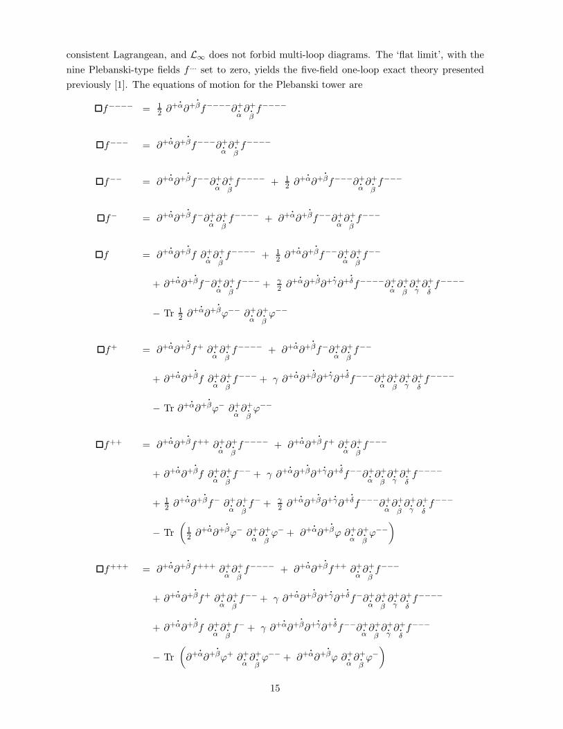
consistent Lagrangean, and L∞ does not forbid multi-loop diagrams. The ‘flat limit’, with the

nine Plebanski-type fields f ... set to zero, yields the five-field one-loop exact theory presented

previously [1]. The equations of motion for the Plebanski tower are

f−−−− = 12 ∂+

.

α∂+.

βf−−−−∂+.

α∂+.

βf−−−−

f−−− = ∂+.

α∂+.

βf−−−∂+.

α∂+.

βf−−−−

f−− = ∂+.

α∂+.

βf−−∂+.

α∂+.

βf−−−− + 1

2 ∂+.

α∂+.

βf−−−∂+.

α∂+.

βf−−−

f− = ∂+.

α∂+.

βf−∂+.

α∂+.

βf−−−− + ∂+

.

α∂+.

βf−−∂+.

α∂+.

βf−−−

f = ∂+.

α∂+.

βf ∂+.

α∂+.

βf−−−− + 1

2 ∂+.

α∂+.

βf−−∂+.

α∂+.

βf−−

+ ∂+.

α∂+.

βf−∂+.

α∂+.

βf−−− + γ

2 ∂+.

α∂+.

β∂+.

γ∂+.

δf−−−−∂+.

α∂+.

β∂+.

γ∂+.

δf−−−−

− Tr 12 ∂+

.

α∂+.

βϕ−− ∂+.

α∂+.

βϕ−−

f+ = ∂+.

α∂+.

βf+ ∂+.

α∂+.

βf−−−− + ∂+

.

α∂+.

βf−∂+.

α∂+.

βf−−

+ ∂+.

α∂+.

βf ∂+.

α∂+.

βf−−− + γ ∂+

.

α∂+.

β∂+.

γ∂+.

δf−−−∂+.

α∂+.

β∂+.

γ∂+.

δf−−−−

− Tr ∂+.

α∂+.

βϕ− ∂+.

α∂+.

βϕ−−

f++ = ∂+.

α∂+.

βf++ ∂+.

α∂+.

βf−−−− + ∂+

.

α∂+.

βf+ ∂+.

α∂+.

βf−−−

+ ∂+.

α∂+.

βf ∂+.

α∂+.

βf−− + γ ∂+

.

α∂+.

β∂+.

γ∂+.

δf−−∂+.

α∂+.

β∂+.

γ∂+.

δf−−−−

+ 12 ∂+

.

α∂+.

βf− ∂+.

α∂+.

βf− + γ

2 ∂+.

α∂+.

β∂+.

γ∂+.

δf−−−∂+.

α∂+.

β∂+.

γ∂+.

δf−−−

− Tr

(12 ∂+

.

α∂+.

βϕ− ∂+.

α∂+.

βϕ− + ∂+

.

α∂+.

βϕ ∂+.

α∂+.

βϕ−−

)

f+++ = ∂+.

α∂+.

βf+++ ∂+.

α∂+.

βf−−−− + ∂+

.

α∂+.

βf++ ∂+.

α∂+.

βf−−−

+ ∂+.

α∂+.

βf+ ∂+.

α∂+.

βf−− + γ ∂+

.

α∂+.

β∂+.

γ∂+.

δf−∂+.

α∂+.

β∂+.

γ∂+.

δf−−−−

+ ∂+.

α∂+.

βf ∂+.

α∂+.

βf− + γ ∂+

.

α∂+.

β∂+.

γ∂+.

δf−−∂+.

α∂+.

β∂+.

γ∂+.

δf−−−

− Tr

(∂+

.

α∂+.

βϕ+ ∂+.

α∂+.

βϕ−− + ∂+

.

α∂+.

βϕ ∂+.

α∂+.

βϕ−

)

15

f++++ = ∂+.

α∂+.

βf++++ ∂+.

α∂+.

βf−−−− + ∂+

.

α∂+.

βf+++ ∂+.

α∂+.

βf−−−

+ ∂+.

α∂+.

βf++ ∂+.

α∂+.

βf−− + ∂+

.

α∂+.

βf+ ∂+.

α∂+.

βf−

+ 12 ∂+

.

α∂+.

βf ∂+.

α∂+.

βf + γ

2 ∂+.

α∂+.

β∂+.

γ∂+.

δf−−∂+.

α∂+.

β∂+.

γ∂+.

δf−−

+ γ ∂+.

α∂+.

β∂+.

γ∂+.

δf−∂+.

α∂+.

β∂+.

γ∂+.

δf−−−

+ γ ∂+.

α∂+.

β∂+.

γ∂+.

δf∂+.

α∂+.

β∂+.

γ∂+.

δf−−−− − Tr

(∂+

.

α∂+.

βϕ++ ∂+.

α∂+.

βϕ−−

+ ∂+.

α∂+.

βϕ+ ∂+.

α∂+.

βϕ− + 1

2 ∂+.

α∂+.

βϕ ∂+.

α∂+.

βϕ

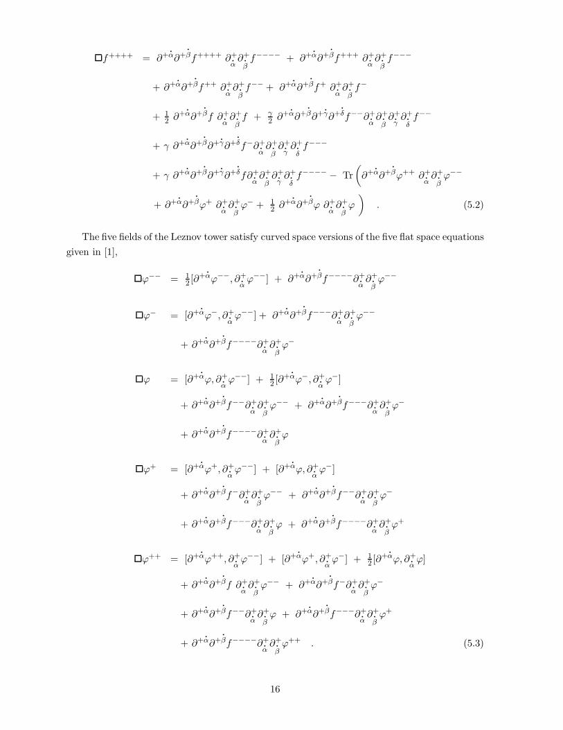
). (5.2)

The five fields of the Leznov tower satisfy curved space versions of the five flat space equations

given in [1],

ϕ−− = 12 [∂+

.

αϕ−−, ∂+.

αϕ−−] + ∂+

.

α∂+.

βf−−−−∂+.

α∂+.

βϕ−−

ϕ− = [∂+.

αϕ−, ∂+.

αϕ−−] + ∂+

.

α∂+.

βf−−−∂+.

α∂+.

βϕ−−

+ ∂+.

α∂+.

βf−−−−∂+.

α∂+.

βϕ−

ϕ = [∂+.

αϕ, ∂+.

αϕ−−] + 1

2 [∂+.

αϕ−, ∂+.

αϕ−]

+ ∂+.

α∂+.

βf−−∂+.

α∂+.

βϕ−− + ∂+

.

α∂+.

βf−−−∂+.

α∂+.

βϕ−

+ ∂+.

α∂+.

βf−−−−∂+.

α∂+.

βϕ

ϕ+ = [∂+.

αϕ+, ∂+.

αϕ−−] + [∂+

.

αϕ, ∂+.

αϕ−]

+ ∂+.

α∂+.

βf−∂+.

α∂+.

βϕ−− + ∂+

.

α∂+.

βf−−∂+.

α∂+.

βϕ−

+ ∂+.

α∂+.

βf−−−∂+.

α∂+.

βϕ + ∂+

.

α∂+.

βf−−−−∂+.

α∂+.

βϕ+

ϕ++ = [∂+.

αϕ++, ∂+.

αϕ−−] + [∂+

.

αϕ+, ∂+.

αϕ−] + 1

2 [∂+.

αϕ, ∂+.

αϕ]

+ ∂+.

α∂+.

βf ∂+.

α∂+.

βϕ−− + ∂+

.

α∂+.

βf−∂+.

α∂+.

βϕ−

+ ∂+.

α∂+.

βf−−∂+.

α∂+.

βϕ + ∂+

.

α∂+.

βf−−−∂+.

α∂+.

βϕ+

+ ∂+.

α∂+.

βf−−−−∂+.

α∂+.

βϕ++ . (5.3)

16

Picture-raising induces a derivation Q+ on the set of target space fields,

Q+ : f−−−− 7→ f−−− 7→ 2 f−− 7→ 3! f− 7→ 4! f 7→ 5! f+ 7→ . . . 7→ 8! f++++

Q+ : ϕ−− 7→ ϕ− 7→ 2 ϕ 7→ 3! ϕ+ 7→ 4! ϕ++ .(5.4)

The five-equation system (5.3) follows from the ϕ−− equation on successive application of Q+.

This property, displayed for the corresponding flat space equations in [1], therefore survives the

coupling to the five f -type fields occurring in (5.3). For the nine-equation tower (5.2), successive

application of Q+ on the ‘top’ (f−−−−) equation yields all the ‘non-stringy’ terms, namely those

not depending on the suppressed α′. On the other hand, these ‘stringy’ terms follow on successive

application of Q+ to the two topological densities inserted in the neutral f equation. However,

the relative normalisations of these two sets of terms are not suited to the consideration of the

f equation as the ‘top’ equation for the positively charged equations.

The fourth-order (γ-dependent) ‘stringy’ terms of the Lagrangean L9+5 are seen to affect

only the equations for the gravitational ‘multiplier’ fields fj≤0 and do not enter the Plebanski

equations for the positive-helicity (negatively-charged) fields. In the high string tension limit,

α′ → 0, these terms in any case disappear and we recover equations which arise on expanding

(2.20). The above 9+5 field system, apart from the α′-dependent deformation, is indeed some-

what similar to self-dual N=8 supergravity [22] plus N=4 self-dual super Yang-Mills [23, 24],

with adjustments made for the difference in statistics of the spinorial fields. We note however,

that whereas the five fields of the Φ−− multiplet are in one-to-one correspondence with the com-

ponents of the N=4 SDYM multiplet [1], the N=8 supermultiplet of [22] has eleven component

fields.

Starting from the 9+5 field truncation, smaller consistent Lagrangean theories may be con-

structed by ignoring any selection of pairs of fields from {(fj , f−j), (ϕj , ϕ−j)}. Any such trunca-

tion of the ‘maximal model’ may easily be seen to be one-loop finite. We note that the ‘minimal

model’, containing only the standard Plebanski and Leznov fields, f−−−− and ϕ−−, together

with their respective multipliers, f++++ and ϕ++, does not even contain a ‘γ-term’.

6 Conclusions

We have seen that the classical curved-space self-duality equations in (2, 2) hyperspace describe

the interaction of open and closed N=2 strings, at least on topologies with χ>0 , up to stringy

torsion-like modifications which vanish in the high tension limit. Since massive N=2 string

excitations do not exist, these α′-corrections are actually unexpected. They owe their appearance

to the picture degeneracy of the massless level, which also forms the basis of the hyperspace

extension of self-duality. The second order α′-terms, moreover, are seen to be indispensable

for the formulation of a unified action principle for the coupled self-dual Einstein-Yang-Mills

system.

In the hyperspace formulation of our coupled system (4.4), the stringy modifications de-

pend explicitly on the spinorial hyperspace coordinates (η±) and do not seem to afford a fully

17

hyperspace-covariant reformulation. This difficulty is actually related to the ‘wrong’ statistics

of the spinorial coordinate. In superspace, the difference in dimension of the two integration

measures, d4θ for the Yang-Mills terms and d8θ for the gravitational ones, makes it possible to

construct a covariant combined action.

The existence of the higher conserved currents and potentials (section 4) seems to indicate

that the α′-deformation introduced here does not affect the integrability of the coupled model.

The full system described by (4.2) therefore deserves further study in this light. Relaxing the

string-enforced requirement of a fixed complex structure, we may recover full Lorentz invariance

in harmonic space, with the {u±α } of section 2 treated as genuine coordinates. It remains to be

seen whether such a reformulation provides an α′-deformation of the Penrose twistor transform.

Acknowledgment

We thank Jurgen Schulze for discussions concerning the relation of string theory to field theory

amplitudes.

References

[1] C. Devchand and O. Lechtenfeld, Extended self-dual Yang-Mills from the N=2 string,

hep-th/9712043, Nucl. Phys. B516 (1998) 255.

[2] O. Lechtenfeld and W. Siegel, N=2 worldsheet instantons yield cubic self-dual Yang-Mills,

hep-th/9704076, Phys. Lett. B405 (1997) 49.

[3] A.N. Leznov, On equivalence of four-dimensional selfduality equations to continual analog

of the main chiral field problem, Theor. Math. Phys. 73 (1988) 1233;

A.N. Leznov and M.A. Mukhtarov, Deformation of algebras and solution of selfduality

equation, J. Math. Phys. 28 (1987) 2574.

[4] A. Parkes, A cubic action for self-dual Yang-Mills,

hep-th/9203074, Phys. Lett. B286 (1992) 265.

[5] D.V. Alekseevsky and V. Cortes, Classification of N -(super)-extended Poincare algebras

and bilinear invariants of the spinor representation of Spin(p, q),

Commun. Math. Phys. 183 (1997) 477.

[6] D. Friedan, E. Martinec and S. Shenker,

Conformal invariance, supersymmetry and string theory, Nucl. Phys. B271 (1986) 93.

[7] J. Bischoff, S.V. Ketov and O. Lechtenfeld,

The GSO projection, BRST cohomology and picture-changing in N=2 string theory,

hep-th/9406101, Nucl. Phys. B438 (1995) 373.

[8] H. Ooguri and C. Vafa, Geometry of N=2 strings, Nucl. Phys. B361 (1991) 469;

Selfduality and N=2 string magic, Mod. Phys. Lett. A5 (1990) 1389.

[9] J. Bischoff and O. Lechtenfeld, Restoring reality for the self-dual N=2 string,

hep-th/9608196, Phys. Lett. B390 (1997) 153.

18

[10] J. Bischoff and O. Lechtenfeld, Path-integral quantization of the (2,2) string,

hep-th/9612218, Int. J. Mod. Phys. A12 (1997) 4933.

[11] N. Marcus,The N=2 open string, hep-th/9207024, Nucl. Phys. B387 (1992) 263;

A tour through N=2 strings, hep-th/9211059.

[12] C. Devchand and V. Ogievetsky, Self-dual gravity revisited,

hep-th/9409160, Class. Quant. Grav. 13 (1996) 2515.

[13] C. Devchand and V. Ogievetsky, Self-dual supergravities,

hep-th/9501061, Nucl. Phys. B444 (1995) 381.

[14] J.F. Plebanski, Some solutions of complex Einstein equations,

J. Math. Phys. 16 (1975) 2395.

[15] M.A. Vasiliev, Consistent equations for interacting massless fields of all spins in the first

order in curvatures, Ann. Phys. 190 (1989) 59.

[16] N. Berkovits and C. Vafa, N=4 topological strings ,

hep-th/9407190, Nucl. Phys. B433 (1995) 123.

[17] K. Junemann and O. Lechtenfeld,

Chiral BRST cohomology of N=2 strings at arbitrary ghost and picture number,

hep-th/9712182.

[18] R. Hippmann, Tree-Level Amplituden des N=2 String, diploma thesis ITP Hannover,

September 1997, http://www.itp.uni-hannover.de/˜lechtenf/Theses/hippmann.ps.

[19] O. Lechtenfeld, Integration measure and spectral flow in the critical N=2 string,

hep-th/9512189, Nucl. Phys. (Proc. Suppl.) B49 (1996) 51.

[20] M. Marquart and J. Schulze, private communication.

[21] C. P. Boyer and J.F. Plebanski, An infinite hierarchy of conservation laws and nonlinear

superposition principles for self-dual Einstein spaces, J. Math. Phys. 26 (1985) 229.

[22] W. Siegel, Self-dual N=8 supergravity as closed N=2(4) strings,

hep-th/9207043, Phys.Rev. D47 (1993) 2504.

[23] W. Siegel, N=2(4) string theory is selfdual N=4 Yang-Mills theory,

hep-th/9205075, Phys. Rev. D46 (1992) 3235.

[24] G. Chalmers and W. Siegel, The selfdual sector of QCD amplitudes,

hep-th/9606061, Phys. Rev. D54 (1996) 7628.

19