arX

iv:h

ep-t

h/04

1208

2v3

1 F

eb 2

005

FTPI-MINN-04/41, UMN-TH-2327/04

NSF-KITP-04-125, ITEP-TH-46/04

IHES-52/04

Non-Abelian Meissner Effect in Yang–Mills

Theories at Weak Coupling

A. Gorsky a,b,c, M. Shifmanb,c and A. Yunga,b,d

aInstitute of Theoretical and Experimental Physics, Moscow 117259, Russia

bWilliam I. Fine Theoretical Physics Institute, University of Minnesota,

Minneapolis, MN 55455, USA

cKavli Institute for Theoretical Physics, UCSB, Santa Barbara, CA 93106, USA

dPetersburg Nuclear Physics Institute, Gatchina, St. Petersburg 188300, Russia

Abstract

We present a weak-coupling Yang–Mills model supporting non-Abelian magnetic flux

tubes and non-Abelian confined magnetic monopoles. In the dual description the mag-

netic flux tubes are prototypes of the QCD strings. Dualizing the confined magnetic

monopoles we get gluelumps which convert a “QCD string” in the excited state to that

in the ground state. Introducing a mass parameter m we discover a phase transition

between the Abelian and non-Abelian confinement at a critical value m = m∗ ∼ Λ.

Underlying dynamics are governed by a ZN symmetry inherent to the model under

consideration. At m > m∗ the ZN symmetry is spontaneously broken, resulting in

N degenerate ZN (Abelian) strings. At m < m∗ the ZN symmetry is restored, the

degeneracy is lifted, and the strings become non-Abelian. We calculate tensions of the

non-Abelian strings, as well as the decay rates of the metastable strings, at N ≫ 1.

Contents

1 Introduction 2

2 In search of non-Abelian strings and monopoles 6

3 The world-sheet theory for the elementary string moduli 11

3.1 Derivation of the CP (N − 1) model . . . . . . . . . . . . . . . . . . . 11

3.2 Penetration of θ from the bulk in the world-sheet theory . . . . . . . 15

4 Dynamics of the world-sheet theory 17

5 Fusing strings 24

6 Kinks are confined monopoles 25

6.1 Breaking SU(N)diag . . . . . . . . . . . . . . . . . . . . . . . . . . . . 25

6.2 Evolution of monopoles . . . . . . . . . . . . . . . . . . . . . . . . . . 28

7 Abelian to non-Abelian string phase transition 30

8 The SU(2)×U(1) case 34

9 Dual picture 38

10 Conclusions 41

1

1 Introduction

Ever since ’t Hooft [1] and Mandelstam [2] put forward the hypothesis of the dual

Meissner effect to explain color confinement in non-Abelian gauge theories people

were trying to find a controllable approximation in which one could reliably demon-

strate the occurrence of the dual Meissner effect in these theories. A breakthrough

achievement was the Seiberg-Witten solution [3] of N = 2 supersymmetric Yang–

Mills theory. They found massless monopoles and, adding a small (N = 2)-breaking

deformation, proved that they condense creating strings carrying a chromoelectric

flux. It was a great success in qualitative understanding of color confinement.

A more careful examination shows, however, that details of the Seiberg-Witten

confinement are quite different from those we expect in QCD-like theories. Indeed,

a crucial aspect of Ref. [3] is that the SU(N) gauge symmetry is first broken, at

a high scale, down to U(1)N−1, which is then completely broken, at a much lower

scale where monopoles condense. Correspondingly, the strings in the Seiberg-Witten

solution are, in fact, Abelian strings [4] of the Abrikosov–Nielsen–Olesen (ANO) type

which results, in turn, in confinement whose structure does not resemble at all that of

QCD. In particular, the “hadronic” spectrum is much richer than that in QCD [5, 6].

Thus, the problem of obtaining the Meissner effect in a more realistic regime in

theories which are closer relatives of QCD remains open. A limited progress in this

direction was achieved since the 1980’s [7]; the advancement accelerated in recent

years [8, 9, 10, 11, 12, 13, 14]. Our task is to combine and distill these advances to

synthesize a relatively simple non-Abelian model exhibiting at least some features of

bona fide non-Abelian confinement in a controllable setting.

What do we know of color confinement in QCD? At a qualitative level surpris-

ingly much. We know that in the Yang–Mills theory chromoelectric flux tubes are

formed between the probe heavy quarks (more exactly, between the quark and its an-

tiquark), with the fundamental tension T1 proportional to the square of the dynamical

2

scale parameter, which does not scale with N at large N ,

T1 ∼ Λ2QCD .

If one pulls together N such flux tubes they can annihilate. This clearly distinguishes

QCD flux tubes from the ANO strings. We know that for k-strings 1 (with k > 1)

excitations lie very close to the ground state. For instance, if one considers two-index

symmetric and antisymmetric sources, the corresponding string tensions T[2] and T{2}

are split [15] by Λ2/N2. The decay rate of the symmetric string into antisymmetric

(per unit length of the string per unit time) is

Γ→

∼ Λ2 exp(

−γ N2)

, (1)

where γ is a positive constant of order one. We would like to model all the above

features at weak coupling, where all approximations made can be checked and ver-

ified. After extensive searches we found seemingly the simplest Yang–Mills model

which does the job, at least to an extent. Our model seems to be minimal. It is

non-supersymmetric. It supports non-Abelian magnetic flux tubes and non-Abelian

confined magnetic monopoles at weak coupling. In the dual description the mag-

netic flux tubes are prototypes of the QCD strings. Dualizing the confined magnetic

monopoles we get gluelumps (string-attached gluons) which convert a “QCD string”

in the excited state to that in the ground state. The decay rate of the excited string

to its ground state is suppressed exponentially in N .

It is worth noting that strings in non-Abelian theories at weak coupling were

found long ago [16] — the so-called ZN strings associated with the center of the

SU(N) gauge group. However, in all these constructions the gauge flux was always

directed along a fixed vector in the Cartan subalgebra of SU(N), and no moduli which

would make the flux orientation a dynamical variable in the group space were ever

found. Therefore, these strings are, in essence, Abelian.1Operationally, k-strings are defined as flux tubes attached to probe sources with k fundamental

or k antifundamental indices.

3

Recently, non-Abelian strings were shown to emerge at weak coupling [10, 11, 13,

14] in N = 2 and deformed N = 4 supersymmetric gauge theories (similar results in

three dimensions were obtained in [9]). The main feature of the non-Abelian strings

is the presence of orientational zero modes associated with the rotation of their color

flux in the non-Abelian gauge group, which makes such strings genuinely non-Abelian.

This is as good as it gets at weak coupling.

In this paper we extend (and simplify) the class of theories in which non-Abelian

strings are supported. To this end we consider a “minimal” non-supersymmetric

gauge theory with the gauge group SU(N)×U(1). Our model is still rather far from

real-world QCD. We believe, however, that our non-Abelian strings capture basic

features of QCD strings to a much greater extent than the Abelian ANO strings.

Striking similarities between four-dimensional gauge theories and two-dimensio-

nal sigma models were noted long ago, in the 1970’s and 80’s. We continue reveal-

ing reasons lying behind these similarities: in fact, two-dimensional sigma models

are effective low-energy theories describing orientational moduli on the world sheet

of non-Abelian confining strings. A particular direct relation was found previously

in N = 2 supersymmetric theories [17, 18, 11, 13] where the BPS kink spectrum

in two-dimensional CP (N − 1) model coincides with the dyon spectrum of a four-

dimensional gauge theory given by the exact Seiberg-Witten solution. Pursuing this

line of research we reveal a similar relationship between non-supersymmetric two- and

four-dimensional theories. The physics of non-supersymmetric sigma models signif-

icantly differs from that of supersymmetric ones. We find interpretations of known

results on non-supersymmetric CP (N − 1) models in terms of non-Abelian strings

and monopoles in four dimensions.

In particular, in parallel to the supersymmetric case [12, 11, 13], we interpret

the confined monopole realizing a junction of two distinct non-Abelian strings, as a

kink in the two-dimensional CP (N − 1) model. The argument is made explicit by

virtue of an extrapolation procedure designed specifically for this purpose. Namely,

4

we introduce mass parameters mA (A = 1, ..., Nf , and Nf = N is the number of bulk

flavors) for scalar quarks in four dimensions. This lifts the orientational moduli of

the string. Now the effective world-sheet description of the string internal dynamics

is given by a massive CP (N − 1) model. In this quasiclassical limit the matching

between the magnetic monopoles and kinks is rather obvious. Tending mA → 0 we

extrapolate this matching to the quantum regime.

In addition to the four-dimensional confinement, that ensures that the magnetic

monopoles are attached to the strings, they are also confined in the two-dimensional

sense. Namely, the monopoles stick to anti-monopoles on the string they are attached

to, to form meson-like configurations. The two-dimensional confinement disappears

if the vacuum angle θ = π. Some monopoles become deconfined along the string.

Alternatively, one can say that strings become degenerate.

With non-vanishing mass terms of the type

{mA} −→ m{

e2πi/N , e4πi/N , ..., e2(N−1)πi/N , 1}

,

a discrete ZN symmetry survives in the effective world-sheet theory. In the domain

of large m (large compared to the scale of the CP (N − 1) model) we have Abelian

strings and essentially the ’t Hooft-Polyakov monopoles, while at small m the strings

and monopoles we deal with become non-Abelian. We show that these two regions are

separated by a phase transition (presumably, of the second order) which we interpret

as a transition between the Abelian and non-Abelian confinement. We show that

in the effective CP (N − 1) model on the string world sheet this phase transition

is associated with the restoration of ZN symmetry: ZN symmetry is broken in the

Abelian confinement phase and restored in the non-Abelian confinement phase. This

is a key result of the present work which has an intriguing (albeit, rather remote)

parallel with the breaking of the ZN symmetry at the confinement/deconfinement

phase transition found in lattice QCD at non-zero temperature.

Next, we consider some special features of the simplest SU(2)×U(1) case. In

5

particular, we discuss the vacuum angle dependence. CP (1) model is known to

become conformal at θ = π, including massless monopoles/kinks at θ = π.

Finally, we focus on the problem of the multiplicity of the hadron spectrum in

the general SU(N)×U(1) case. As was already mentioned, the Abelian confinement

generates too many hadron states as compared to QCD-based expectations [5, 6, 19].

In our model this regime occurs at large mA.

2 In search of non-Abelian strings and monopoles

A reference model which we suggest for consideration is quite simple. The gauge group

of the model is SU(N)×U(1). Besides SU(N) and U(1) gauge bosons the model

contains N scalar fields charged with respect to U(1) which form N fundamental

representations of SU(N). It is convenient to write these fields in the form of N ×N

matrix Φ = {ϕkA} where k is the SU(N) gauge index while A is the flavor index,

Φ =

ϕ11 ϕ12 ... ϕ1N

ϕ21 ϕ22 ... ϕ2N

... ... ... ...

ϕN1 ϕN2 ... ϕNN

. (2)

Sometimes we will refer to ϕ’s as to scalar quarks, or just quarks. The action of the

model has the form 2

S =∫

d4x

{

1

4g22

(

F aµν

)2+

1

4g21

(Fµν)2

+ Tr (∇µΦ)† (∇µΦ) +g22

2

[

Tr(

Φ†T aΦ)]2

+g21

8

[

Tr(

Φ†Φ)

− Nξ]2

2Here and below we use a formally Euclidean notation, e.g. F 2

µν = 2F 2

0i + F 2

ij , (∂µa)2 =

(∂0a)2 + (∂ia)2, etc. This is appropriate since we are going to study static (time-independent)

field configurations, and A0 = 0. Then the Euclidean action is nothing but the energy functional.

6

+i θ

32 π2F a

µνFaµν

}

, (3)

where T a stands for the generator of the gauge SU(N),

∇µ Φ ≡(

∂µ − i√2N

Aµ − iAaµ T a

)

Φ , (4)

(the global flavor SU(N) transformations then act on Φ from the right), and θ is

the vacuum angle. The action (3) in fact represents a truncated bosonic sector of

the N = 2 model. The last term in the second line forces Φ to develop a vacuum

expectation value (VEV) while the last but one term forces the VEV to be diagonal,

Φvac =√

ξ diag {1, 1, ..., 1} . (5)

In this paper we assume the parameter ξ to be large,3

√

ξ ≫ Λ4, (6)

where Λ4 is the scale of the four-dimensional theory (3). This ensures the weak

coupling regime as both couplings g21 and g2

2 are frozen at a large scale.

The vacuum field (5) results in the spontaneous breaking of both gauge and

flavor SU(N)’s. A diagonal global SU(N) survives, however, namely

U(N)gauge × SU(N)flavor → SU(N)diag . (7)

Thus, color-flavor locking takes place in the vacuum. A version of this scheme of

symmetry breaking was suggested long ago [20].

Now, let us briefly review string solutions in this model. Since it includes a

spontaneously broken gauge U(1), the model supports conventional ANO strings [4]

in which one can discard the SU(N)gauge part of the action. The topological stability

of the ANO string is due to the fact that π1(U(1)) = Z. These are not the strings we

are interested in. At first sight the triviality of the homotopy group, π1(SU(N)) = 0,

3The reader may recognize ξ as a descendant of the Fayet–Iliopoulos parameter.

7

implies that there are no other topologically stable strings. This impression is false.

One can combine the ZN center of SU(N) with the elements exp(2πik/N) ∈U(1)

to get a topologically stable string solution possessing both windings, in SU(N) and

U(1). In other words,

π1 (SU(N) × U(1)/ZN) 6= 0 . (8)

It is easy to see that this nontrivial topology amounts to winding of just one element

of Φvac, say, ϕ11, or ϕ22, etc, for instance,4

Φstring =√

ξ diag(1, 1, ..., eiα(x)) , x → ∞ . (9)

Such strings can be called elementary; their tension is 1/N -th of that of the ANO

string. The ANO string can be viewed as a bound state of N elementary strings.

More concretely, the ZN string solution (a progenitor of the non-Abelian string)

can be written as follows [10]:

Φ =

φ(r) 0 ... 0

... ... ... ...

0 ... φ(r) 0

0 0 ... eiαφN(r)

,

ASU(N)i =

1

N

1 ... 0 0

... ... ... ...

0 ... 1 0

0 0 ... −(N − 1)

(∂iα) [−1 + fNA(r)] ,

AU(1)i =

1

N(∂iα) [1 − f(r)] , A

U(1)0 = A

SU(N)0 = 0 , (10)

where i = 1, 2 labels coordinates in the plane orthogonal to the string axis and r and α

are the polar coordinates in this plane. The profile functions φ(r) and φN(r) determine

4As explained below, α is the angle of the coordinate ~x⊥ in the perpendicular plane.

8

the profiles of the scalar fields, while fNA(r) and f(r) determine the SU(N) and U(1)

fields of the string solutions, respectively. These functions satisfy the following rather

obvious boundary conditions:

φN(0) = 0,

fNA(0) = 1, f(0) = 1 , (11)

at r = 0, and

φN(∞) =√

ξ, φ(∞) =√

ξ ,

fNA(∞) = 0, f(∞) = 0 (12)

at r = ∞. Because our model is equivalent, in fact, to a bosonic reduction of the N =

2 supersymmetric theory, these profile functions satisfy the first-order differential

equations obtained in [21], namely,

rd

drφN(r) − 1

N(f(r) + (N − 1)fNA(r))φN(r) = 0 ,

rd

drφ(r) − 1

N(f(r) − fNA(r))φ(r) = 0 ,

−1

r

d

drf(r) +

g21N

4

[

(N − 1)φ(r)2 + φN(r)2 − Nξ]

= 0 ,

−1

r

d

drfNA(r) +

g22

2

[

φN(r)2 − φ2(r)2]

= 0 . (13)

These equations can be solved numerically. Clearly, the solutions to the first-order

equations automatically satisfy the second-order equations of motion. Quantum cor-

rections destroy fine-tuning of the coupling constants in (3). If one is interested in

calculation of the quantum-corrected profile functions one has to solve the second-

order equations of motion instead of (13).

The tension of this elementary string is

T1 = 2π ξ . (14)

9

As soon as our theory is not supersymmetric and the string is not BPS there are

corrections to this result which are small and uninteresting provided the coupling

constants g21 and g2

2 are small. Note that the tension of the ANO string is

TANO = 2π N ξ (15)

in our normalization.

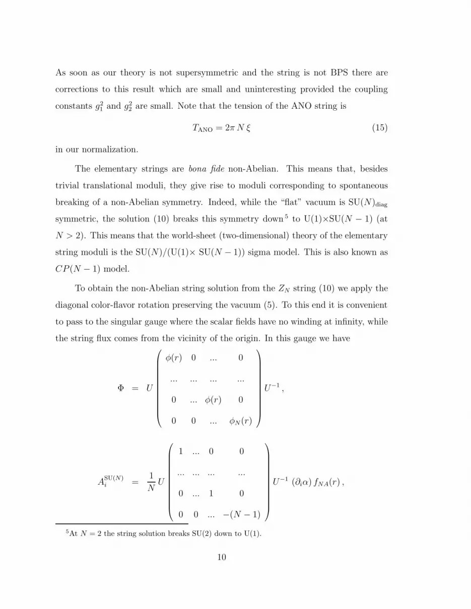
The elementary strings are bona fide non-Abelian. This means that, besides

trivial translational moduli, they give rise to moduli corresponding to spontaneous

breaking of a non-Abelian symmetry. Indeed, while the “flat” vacuum is SU(N)diag

symmetric, the solution (10) breaks this symmetry down 5 to U(1)×SU(N − 1) (at

N > 2). This means that the world-sheet (two-dimensional) theory of the elementary

string moduli is the SU(N)/(U(1)× SU(N − 1)) sigma model. This is also known as

CP (N − 1) model.

To obtain the non-Abelian string solution from the ZN string (10) we apply the

diagonal color-flavor rotation preserving the vacuum (5). To this end it is convenient

to pass to the singular gauge where the scalar fields have no winding at infinity, while

the string flux comes from the vicinity of the origin. In this gauge we have

Φ = U

φ(r) 0 ... 0

... ... ... ...

0 ... φ(r) 0

0 0 ... φN(r)

U−1 ,

ASU(N)i =

1

NU

1 ... 0 0

... ... ... ...

0 ... 1 0

0 0 ... −(N − 1)

U−1 (∂iα) fNA(r) ,

5At N = 2 the string solution breaks SU(2) down to U(1).

10

AU(1)i = − 1

N(∂iα) f(r) , A

U(1)0 = A

SU(N)0 = 0 , (16)

where U is a matrix ∈ SU(N). This matrix parametrizes orientational zero modes

of the string associated with flux rotation in SU(N). The presence of these modes

makes the string genuinely non-Abelian. Since the diagonal color-flavor symmetry is

not broken by the vacuum expectation values (VEV’s) of the scalar fields in the bulk

(color-flavor locking) it is physical and has nothing to do with the gauge rotations

eaten by the Higgs mechanism. The orientational moduli encoded in the matrix U

are not gauge artifacts. The orientational zero modes of a non-Abelian string were

first observed in [9, 10].

3 The world-sheet theory for the elementary string

moduli

In this section we will present derivation of an effective low-energy theory for the

orientational moduli of the elementary string and then discuss underlying physics.

We will closely follow Refs. [10, 11] where this derivation was carried out for N = 2

which leads to the CP (1) model. In the general case, as was already mentioned, the

resulting macroscopic theory is a two-dimensional CP (N − 1) model [9, 10, 11, 13].

3.1 Derivation of the CP (N − 1) model

First, extending the supersymmetric CP (1) derivation of Refs. [10, 11], we will derive

the effective low-energy theory for the moduli residing in the matrix U in the problem

at hand. As is clear from the string solution (16), not each element of the matrix U

will give rise to a modulus. The SU(N − 1)×U(1) subgroup remains unbroken by the

string solution under consideration; therefore, as was already mentioned, the moduli

11

space isSU(N)

SU(N − 1) × U(1)∼ CP (N − 1) . (17)

Keeping this in mind we parametrize the matrices entering Eq. (16) as follows:

1

N

U

1 ... 0 0

... ... ... ...

0 ... 1 0

0 0 ... −(N − 1)

U−1

l

p

= −nln∗p +

1

Nδlp , (18)

where nl is a complex vector in the fundamental representation of SU(N), and

n∗l n

l = 1 ,

(l, p = 1, ..., N are color indices). As we will show below, one U(1) phase will be

gauged in the effective sigma model. This gives the correct number of degrees of

freedom, namely, 2(N − 1).

With this parametrization the string solution (16) can be rewritten as

Φ =1

N[(N − 1)φ + φN ] − (φ − φN)

(

n · n∗ − 1

N

)

,

ASU(N)i =

(

n · n∗ − 1

N

)

εijxi

r2fNA(r) ,

AU(1)i =

1

Nεij

xi

r2f(r) , (19)

where for brevity we suppress all SU(N) indices. The notation is self-evident.

Assume that the orientational moduli are slowly-varying functions of the string

world-sheet coordinates xα, α = 0, 3. Then the moduli nl become fields of a (1+1)-

dimensional sigma model on the world sheet. Since nl parametrize the string zero

modes, there is no potential term in this sigma model.

To obtain the kinetic term we substitute our solution (19), which depends on

the moduli nl, in the action (3), assuming that the fields acquire a dependence on

12

the coordinates xα via nl(xα). In doing so we immediately observe that we have to

modify the solution including in it the α = 0, 3 components of the gauge potential

which are no more vanishing. In the CP (1) case, as was shown in [11], the potential

Aα must be orthogonal (in the SU(N) space) to the matrix (18) as well as to its

derivatives with respect to xα. Generalization of these conditions to the CP (N − 1)

case leads to the following ansatz:

ASU(N)α = −i [∂αn · n∗ − n · ∂αn∗ − 2n · n∗(n∗∂αn)] ρ(r) , α = 0, 3 , (20)

where we assume the contraction of the color indices inside the parentheses,

(n∗∂αn) ≡ n∗l ∂αnl ,

and introduce a new profile function ρ(r).

The function ρ(r) in Eq. (20) is determined through a minimization procedure

[10, 11] which generates ρ’s own equation of motion. Now we derive it. But at first

we note that ρ(r) vanishes at infinity,

ρ(∞) = 0 . (21)

The boundary condition at r = 0 will be determined shortly.

The kinetic term for nl comes from the gauge and quark kinetic terms in Eq. (3).

Using Eqs. (19) and (20) to calculate the SU(N) gauge field strength we find

FSU(N)αi = (∂αn · n∗ + n · ∂αn∗) εij

xj

r2fNA [1 − ρ(r)]

+ i [∂αn · n∗ − n · ∂αn∗ − 2n · n∗(n∗∂αn)]xi

r

d ρ(r)

dr. (22)

In order to have a finite contribution from the term Tr F 2αi in the action we have to

impose the constraint

ρ(0) = 1 . (23)

Substituting the field strength (22) in the action (3) and including, in addition, the

kinetic term of the quarks, after a rather straightforward but tedious algebra we arrive

13

at

S(1+1) = 2β∫

dt dz{

(∂α n∗∂α n) + (n∗∂α n)2}

, (24)

where the coupling constant β is given by

β =2π

g22

I , (25)

and I is a basic normalizing integral

I =∫ ∞

0rdr

(

d

drρ(r)

)2

+1

r2f 2

NA (1 − ρ)2

+ g22

[

ρ2

2

(

φ2 + φ2N

)

+ (1 − ρ) (φ − φN)2

]}

. (26)

The theory in Eq. (24) is in fact the two-dimensional CP (N − 1) model. To

see that this is indeed the case we can eliminate the second term in (24) by virtue of

introduction of a non-propagating U(1) gauge field. We review this in Sect. 4, and

then discuss the underlying physics of the model. Thus, we obtain the CP (N − 1)

model as an effective low-energy theory on the world sheet of the non-Abelian string.

Its coupling β is related to the four-dimensional coupling g22 via the basic normalizing

integral (26). This integral can be viewed as an “action” for the profile function ρ.

Varying (26) with respect to ρ one obtains the second-order equation which the

function ρ must satisfy, namely,

− d2

dr2ρ − 1

r

d

drρ − 1

r2f 2

NA (1 − ρ) +g22

2

(

φ2N + φ2

)

ρ − g22

2(φN − φ)2 = 0 . (27)

After some algebra and extensive use of the first-order equations (13) one can show

that the solution of (27) is given by

ρ = 1 − φN

φ. (28)

This solution satisfies the boundary conditions (21) and (23).

Substituting this solution back in the expression for the normalizing integral (26)

one can check that this integral reduces to a total derivative and is given by the flux

14

of the string determined by fNA(0) = 1. Therefore, we arrive at

I = 1 . (29)

This result can be traced back to the fact that our theory (3) is a bosonic reduction

of the N = 2 supersymmetric theory, and the string satisfies the first-order equations

(13) (see [11] for the explanation why (29) should hold for the BPS non-Abelian

strings in SUSY theories). The fact that I = 1 was demonstrated previously for

N = 2, where the CP (1) model emerges. Generally speaking, for non-BPS strings,

I could be a certain function of N (see Ref. [14] for a particular example). In the

problem at hand it is N -independent. However, we expect that quantum corrections

slightly modify Eq. (29).

The relation between the four-dimensional and two-dimensional coupling con-

stants (25) is obtained at the classical level. In quantum theory both couplings

run. So we have to specify a scale at which the relation (25) takes place. The two-

dimensional CP (N − 1) model (24) is an effective low-energy theory good for the

description of internal string dynamics at small energies, much less than the inverse

thickness of the string which is given by√

ξ. Thus,√

ξ plays the role of a physical

ultraviolet (UV) cutoff in (24). This is the scale at which Eq. (25) holds. Below this

scale, the coupling β runs according to its two-dimensional renormalization-group

flow, see the next section.

3.2 Penetration of θ from the bulk in the world-sheet theory

Now let us investigate the impact of the θ term that is present in our microscopic

theory (3). At first sight, seemingly it cannot produce any effect because our string

is magnetic. However, if one allows for slow variations of nl with respect to z and

t, one immediately observes that the electric field is generated via A0,3 in Eq. (20).

Substituting Fαi from (22) into the θ term in the action (3) and taking into account

the contribution from Fαγ times Fij (α, γ = 0, 3 and i, j = 1, 2) we get the topological

15

term in the effective CP (N − 1) model (24) in the form

S(1+1) =∫

dt dz

{

2β[

(∂α n∗∂α n) + (n∗∂α n)2]

− θ

2πIθ εαγ (∂α n∗∂γ n)

}

, (30)

where Iθ is another normalizing integral given by the formula

Iθ = −∫

dr

{

2fNA(1 − ρ)dρ

dr+ (2ρ − ρ2)

df

dr

}

=∫

drd

dr

{

2fNA ρ − ρ2 fNA

}

. (31)

As is clearly seen, the integrand here reduces to a total derivative, and the inte-

gral is determined by the boundary conditions for the profile functions ρ and fNA.

Substituting (21), (23) and (12), (11) we get

Iθ = 1 , (32)

independently of the form of the profile functions. This latter circumstance is perfectly

natural for the topological term.

The additional term (30) in the CP (N − 1) model that we have just derived is

the θ term in the standard normalization. The result (32) could have been expected

since physics is 2π-periodic with respect to θ both in the four-dimensional microscopic

gauge theory and in the effective two-dimensional CP (N − 1) model. The result (32)

is not sensitive to the presence of supersymmetry. It will hold in supersymmetric

models as well. Note that the complexified bulk coupling constant converts into the

complexified world-sheet coupling constant,

τ =4π

g22

+ iθ

2π→ 2β + i

θ

2π.

The above derivation provides the first direct calculation proving the coincidence

of the θ angles in four and two dimensions.

Let us make a comment on this point from the brane perspective. Since the model

under consideration is non-supersymmetric, the usual brane picture corresponding to

16

minimal surfaces in the external geometry is complicated and largely unavailable at

present. However, a few statements insensitive to details of the brane picture can be

made — the identification of the θ angles in the microscopic and microscopic theories

above is one of them. Indeed, in any relevant brane picture the θ angle corresponds

to the distance between two M5 branes along the eleventh dimension in M-theory

[22]. The four-dimensional theory is defined on the world-volume of one of these M5

branes, while an M2 brane stretched between M5 branes corresponds to the non-

Abelian string we deal with. It is clear that the θ angles are the same since it is

just the same geometrical parameter viewed from two different objects: M5 and M2

branes (see also Footnote 7 in Ref. [13]).

4 Dynamics of the world-sheet theory

The CP (N −1) model describing the string moduli interactions can be cast in several

equivalent representations. The most convenient for our purposes is a linear gauged

representation (for a review see [23]). At large N the model was solved [24, 25].

In this formulation the Lagrangian is built from an N -component complex field

nℓ subject to the constraint

n∗ℓ nℓ = 1 , (33)

The Lagrangian has the form

L =2

g2

[

(∂α + iAα) n∗ℓ (∂α − iAα)nℓ − λ

(

n∗ℓn

ℓ − 1)]

, (34)

where 1/g2 ≡ β and λ is the Lagrange multiplier enforcing (33). Moreover, Aα is an

auxiliary field which enters the Lagrangian with no kinetic term. Eliminating Aα by

virtue of the equations of motion one arrives at Eq. (30).

At the quantum level the constraint (33) is gone; λ becomes dynamical. More-

over, a kinetic term is generated for the auxiliary field Aα at the quantum level, so

that Aα becomes dynamical too.

17

Vacuum energy

k0−1−2 1 2

Figure 1: The vacuum structure of CP (N − 1) model at θ = 0.

As was shown above, the θ term which can be written as

Lθ =θ

2πεαγ∂

αAγ =θ

2πεαγ∂

α(

n∗ℓ∂

γnℓ)

(35)

appears in the world-sheet theory of the string moduli provided the same θ angle is

present in the bulk (microscopic) theory.

Now we have to discuss the vacuum structure of the theory (34). Basing on a

modern understanding of the issue [26] (see also [27]) one can say that for each θ

there are infinitely many “vacua” that are stable in the limit N → ∞. The word

“vacua” is in the quotation marks because only one of them presents a bona fide

global minimum; others are local minima and are metastable at finite (but large) N .

A schematic picture of these vacua is given in Fig. 1. All these minima are entangled

in the θ evolution. If we vary θ continuously from 0 to 2π the depths of the minima

“breathe.” At θ = π two vacua become degenerate (Fig. 2), while for larger values of θ

the global minimum becomes local while the adjacent local minimum becomes global.

The splitting between the values of the consecutive minima is of the order of 1/N ,

while the the probability of the false vacuum decay is proportional to N−1 exp(−N),

see below.

As long as the CP (N − 1) model plays a role of the effective theory on the

world sheet of non-Abelian string each of these “vacua” corresponds to a string in

the four-dimensional bulk theory. For each given θ, the ground state of the string is

18

Figure 2: The vacuum structure of CP (N − 1) model at θ = π.

described by the deepest vacuum of the world-sheet theory, CP (N − 1). Metastable

vacua of CP (N − 1) correspond to excited strings.

As was shown by Witten [24], the field nℓ can be viewed as a field describing

kinks interpolating between the true vacuum and its neighbor. The multiplicity of

such kinks is N [28], they form an N -plet. This is the origin of the superscript ℓ in

nℓ.

Moreover, Witten showed, by exploiting 1/N expansion to the leading order,

that a mass scale is dynamically generated in the model, through dimensional trans-

mutation,

Λ2 = M20 exp

(

− 8π

Ng2

)

. (36)

Here M0 is the ultraviolet cut-off (for the effective theory on the string world sheet

M0 =√

ξ) and g2 = 1/β is the bare coupling constant given in Eq. (25). The

combination Ng2 is nothing but the ’t Hooft constant that does not scale with N .

As a result, Λ scales as N0 at large N .

In the leading order, N0, the kink mass Mn is θ-independent,

Mn = Λ . (37)

θ-dependent corrections to this formula appear only at the level 1/N2.

The kinks represented in the Lagrangian (34) by the field nℓ are not asymptotic

states in the CP (N − 1) model. In fact, they are confined [24]; the confining po-

19

n

k=0

n

k=0

*

k=1������

������

���������

���������

Figure 3: Linear confinement of the n-n∗ pair. The solid straight line represents the

string. The dashed line shows the vacuum energy density (normalizing E0 to zero).

tential grows linearly with distance 6, with the tension suppressed by 1/N . From the

four-dimensional perspective the coefficient of the linear confinement is nothing but

the difference in tensions of two strings: the lightest and the next one, see below.

Therefore, we denote it as ∆T ,

∆T = 12πΛ2

N. (38)

One sees that confinement becomes exceedingly weak at large N . In fact, Eq. (38)

refers to θ = 0. The standard argument that θ dependence does not appear at

N → ∞ is inapplicable to the string tension, since the string tension itself vanishes

in the large-N limit. The θ dependence can be readily established from a picture of

the kink confinement discussed in [14], see Fig. 3, which is complementary to that of

[24]. This picture of the kink confinement is schematically depicted in this figure.

Since the kink represents an interpolation between the genuine vacuum and a

false one, the kink–anti-kink configuration presented in Fig. 3 shows two distinct

regimes: the genuine vacuum outside the kink–anti-kink pair and the false one inside.

As was mentioned, the string tension ∆T is given by the difference of the vacuum

energy densities, that of the the false vacuum minus the genuine one. At large N ,

the k dependence of the energy density in the “vacua” (k is the excitation number),

6Let us note in passing that corrections to the leading-order result (38) run in powers of 1/N2

rather than 1/N . Indeed, as well-known, the θ dependence of the vacuum energy enters only through

the combination of θ/N , namely E(θ) = NΛ2f(θ/N) where f is some function. As will be explained

momentarily, ∆T = E(θ = 2π) − E(θ = 0). Moreover, E , being CP even, can be expanded in even

powers of θ. This concludes the proof that ∆T = (12πΛ2/N)(1 +∑∞

k=1ckN−2k).

20

k=1

n *

k=0

n

k=1������

������

���������

���������

Figure 4: Breaking of the excited string through the n-n∗ pair creation. The dashed

line shows the vacuum energy density.

as well as the θ dependence, is well-known [26],

Ek(θ) = −6

πN Λ2

1 − 1

2

(

2πk + θ

N

)2

. (39)

At θ = 0 the genuine vacuum corresponds to k = 0, while the first excitation to

k = −1. At θ = π these two vacua are degenerate, at θ = 2π their roles interchange.

Therefore,

∆T (θ) = 12πΛ2

N

∣

∣

∣

∣

∣

1 − θ

π

∣

∣

∣

∣

∣

. (40)

Note that at θ = π the string tension vanishes and confinement of kinks disappears.

This formula requires a comment which we hasten to make. In fact, for each

given θ, there are two types of kinks which are degenerate at θ = 0 but acquire

a splitting at θ 6= 0. This is clearly seen in Fig. 5 which displays E0,±1 for three

minima: the global one (k = 0) and two adjacent local minima, k = ±1 (the above

nomenclature refers to |θ| < π). Let us consider, say, small and positive values of

θ. Then the kink described by the field n can represent two distinct interpolations:

from the ground state to the state k = −1 (i.e. the minimum to the left of the global

minimum in Fig. 1); then

∆E =12πΛ2

N

(

1 − θ

π

)

.

Another possible interpolation is from the ground state to the state k = 1 (i.e. the

minimum to the right of the global minimum in Fig. 1). In the latter case

∆E =12πΛ2

N

(

1 +θ

π

)

.

In the first scenario the string becomes tensionless 7, i.e. the states k = 0,−1 degen-

erate, at θ = π. The same consideration applies to negative values of θ. Now it is7Note that in Witten’s work [24] there is a misprint in Eq. (18) and subsequent equations; the

21

k=0

θ/π

k= 1k=1

-2 -1 1 2

1

2

3

4

5

Figure 5: The function 1 + E0,±1/[(6N Λ2)π−1] in the units π2/(2N2) versus θ/π.

the vacua k = 0, 1 that become degenerate at θ = −π, rendering the corresponding

string tensionless. In general, it is sufficient to consider the interval |θ| ≤ π.

What will happen if we interchange the position of two kinks in Fig. 3 , as

shown in Fig. 4? The excited vacuum is now outside the kink-anti-kink pair, while

the genuine one is inside. Formally, the string tension becomes negative. In fact, the

process in Fig. 4 depicts a breaking of the excited string. As was mentioned above, the

probability of such breaking is suppressed by exp(−N). Indeed, the master formula

from Ref. [29] implies that the probability of the excited string decay (through the

n-n∗ pair creation) per unit time per unit length is

Γ =∆T

2πexp

(

−πM2n

∆T

)

=6Λ2

Ne−N/12 (41)

at θ = 0. At θ 6= 0 the suppression is even stronger.

To summarize, the CP (N − 1) model has a fine structure of “vacua” which are

split, with the splitting of the order of Λ2/N . In four-dimensional bulk theory these

“vacua” correspond to elementary non-Abelian strings. Classically all these strings

have the same tension (14). Due to quantum effects in the world-sheet theory the

factor θ/2π should be replaced by θ/π. Two types of kinks correspond in this equation to x > y and

x < y, respectively.

22

degeneracy is lifted: the elementary strings become split, with the tensions

T = 2πξ − 6

πN Λ2

1 − 1

2

(

2πk + θ

N

)2

. (42)

Note that (i) the splitting does not appear to any finite order in the coupling constants;

(ii) since ξ ≫ Λ, the splitting is suppressed in both parameters, Λ/√

ξ and 1/N .

Let us also note that the identification of the θ terms and topological charges in

two and four dimensions (see Sect. 3.2) allows us to address the issue of CP symmetry

in four dimensions at θ = π, and confront it with the situation in two dimensions, see

Ref. [30]. In this work it was shown, on the basis of strong coupling analysis, that

there is a cusp in the partition function of the CP (N − 1) model at θ = π, implying

that the expectation value of the two-dimensional topological charge does not vanish

at this point. This tells us that CP -invariance is dynamically spontaneously broken

at θ = π.

The above result is in full agreement with Witten’s picture of the vacuum family

in the CP (N − 1) model, with N states — one global minimum, other local ones

— entangled in the θ evolution. At θ = π two minima are degenerate, but they are

characterized by opposite values of the topological charge VEV’s,

〈εαγ∂αn∗

ℓ ∂γnℓ〉 = ±Λ2 .

The kink (confined monopole) can be viewed as a barrier separating two domains

(two degenerate strings) carrying opposite CP .

On the other hand, the bulk four-dimensional theory is weakly coupled, and for

each given θ the bulk vacuum is unique. There is no spontaneous CP violation in

the four-dimensional bulk theory at θ = π. One can easily check this assertion by

carrying out a direct instanton calculation.

23

5 Fusing strings

As has been already mentioned, in QCD one can consider not only basic strings, but

2-strings, 3-strings, ... , k-strings, and their excitations. k-strings are composite flux

tubes attached to color sources with N -ality k. Moreover, the N -string ensembles

— i.e. N -strings — can decay into a no-string state. It is natural to ask how these

phenomena manifest themselves in the model under consideration.

If the ansatz (9) defines a basic string, it is not difficult to generalize this defini-

tion to get an analog of 2-strings, 3-strings, etc., for instance,

Φ2−string =√

ξ diag (eiα(x), eiα(x) , 1, ..., 1) , x → ∞ . (43)

The solution (43) breaks SU(N) symmetry down to U(1)×SU(2)×SU(N − 2) (at

N > 3). This means that the world-sheet (two-dimensional) theory of the string

moduli is the SU(N)/(U(1)×SU(2)×SU(N − 2)) sigma model. This is also known as

the Grassmannian G2,N model. At large N it has more fields, by a factor of 2, than

the CP (N − 1) model; other features are quite similar.

The statement that in our model the world-sheet theory for k-strings is the

Grassmannian Gk,N model has a clear-cut indirect confirmation. Indeed, the k-string

ansatz of the type indicated in Eq. (43) tells us that the number of distinct classical

strings is

ν(k, N) = CNk =

N !

k!(N − k)!, (44)

since k phase factors eiα can be distributed arbitrarily in N positions. From the

two-dimensional perspective this number should match the number of distinct vacua

of the world-sheet theory. The latter was calculated in supersymmetric Gk,N model

in Ref. [31], where it was shown to be CNk , as in Eq. (44). In supersymmetric Gk,N

model all these vacua are degenerate, i.e. we have degenerate strings. Introducing

supersymmetry breaking we move away from the degeneracy. In non-supersymmetric

Gk,N model, the number ν(k, N) = CNk gives the number of states in the vacuum

24

family: the genuine vacuum plus metastable ones entangled with the genuine vacuum

in the θ evolution.

As soon as string tensions in our model are classically determined by their U(1)

charges the tension of k-string is given by

Tk = 2π k ξ + O(Λ2), (45)

where corrections of order of Λ2 are induced by the quantum effects in the effective

world sheet theory.

If we add up N strings, the resulting conglomerate is connected to the ANO

string.

6 Kinks are confined monopoles

The CP (N − 1) models are asymptotically free theories and flow to strong coupling

in the infrared. Therefore, the non-Abelian strings discussed in the previous sec-

tions are in a highly quantum regime. To make contact with the classical Abelian

strings we can introduce parameters which explicitly break the diagonal color-flavor

SU(N)diag symmetry lifting the orientational string moduli. This allows us to obtain

a quasiclassical interpretation of the confined monopoles as string junctions, and fol-

low their evolution from (almost) ’t Hooft–Polyakov monopoles to highly quantum

sigma-model kinks. In the supersymmetric case this was done in Refs. [12, 11, 13].

6.1 Breaking SU(N)diag

In order to trace the monopole evolution we modify our basic model (3) introducing,

in addition to the already existing fields, a complex adjoint scalar field aa,

S =∫

d4x

{

1

4g22

(

F aµν

)2+

1

4g21

(Fµν)2 +

1

g22

|Dµaa|2

25

+ Tr (∇µΦ)† (∇µΦ) +g22

2

[

Tr(

Φ†T aΦ)]2

+g21

8

[

Tr(

Φ†Φ)

− Nξ]2

+1

2Tr

∣

∣

∣aaT a Φ + Φ√

2M∣

∣

∣

2+

i θ

32 π2F a

µνFa µν

}

, (46)

where Dµ is a covariant derivative acting in the adjoint representation of SU(N) and

M is a mass matrix for scalar quarks Φ. We assume that it has a diagonal form

M =

m1 ... 0

... ... ...

0 ... mN

, (47)

with the vanishing sum of the diagonal entries,

N∑

A=1

mA = 0 . (48)

Later on it will be convenient to make a specific choice of the parameters mA, namely,

M = m × diag{

e2πi/N , e4πi/N , ..., e2(N−1)πi/N , 1}

, (49)

where m is a single common parameter, and the constraint (48) is automatically

satisfied. We can (and will) assume m to be real and positive.

In fact, the model (46) presents a less reduced bosonic part of the N = 2 super-

symmetric theory than the model (3) on which we dwelled above. In the N =

2 supersymmetric theory the adjoint field is a part of N = 2 vector multiplet. For

the purpose of the string solution the field aa is sterile as long as mA = 0. Therefore,

it could be and was ignored in the previous sections. However, if one’s intention is to

connect oneself to the quasiclassical regime, mA 6= 0, and the adjoint field must be

reintroduced.

For the reason which will become clear shortly, let us assume that, although

mA 6= 0, they are all small compared to√

ξ,

m ≪√

ξ ,

26

but m ≫ Λ. For generic non-degenerate values of mA the adjoint field develops

VEV’s,

〈a〉 = −√

2

m1 ... 0

... ... ...

0 ... mN

. (50)

The vacuum expectation values of the scalar quarks Φ remain intact; they are given

by Eq. (5). For the particular choice specified in Eq. (49)

〈a〉 = −√

2m diag{

e2πi/N , e4πi/N , ..., e2(N−1)πi/N , 1}

. (51)

Clearly the diagonal color-flavor group SU(N)diag is now broken by adjoint VEV’s

down to U(1)N−1 × ZN . Still, the solutions for the Abelian (or ZN) strings are the

same as was discussed in Sect. 2 since the adjoint field does not enter these solutions.

In particular, we have N distinct ZN string solutions depending on what particular

squark winds at infinity, see Sect. 2. Say, the string solution with the winding last

flavor is still given by Eq. (10).

What is changed with the color-flavor SU(N)diag explicitly broken by mA 6= 0,

the rotations (16) no more generate zero modes. In other words, the fields nℓ become

quasi-moduli: a shallow potential for the quasi-moduli nl on the string world sheet is

generated. This potential is shallow as long as mA ≪ √ξ.

This potential was calculated in the CP (1) case in Ref. [11]; the CP (N −1) case

was treated in [13]. It has the following form:

VCP (N−1) = 2β

∑

l

|ml|2|nl|2 −∣

∣

∣

∣

∣

∑

l

ml|nl|2∣

∣

∣

∣

∣

2

. (52)

The potential simplifies if the mass terms are chosen according to (49),

VCP (N−1) = 2β m2

1 −∣

∣

∣

∣

∣

N∑

ℓ=1

e2πi ℓ/N |nℓ|2∣

∣

∣

∣

∣

2

. (53)

This potential is obviously invariant under the cyclic substitution

ℓ → ℓ + k , nℓ → nℓ+k , ∀ ℓ , (54)

27

with k fixed. This property will be exploited below.

Now our effective two-dimensional theory on the string world sheet becomes a

massive CP (N − 1) model. The potential (52) or (53) has N vacua at

nℓ = δℓℓ0 , ℓ0 = 1, 2, ..., N . (55)

These vacua correspond to N distinct Abelian ZN strings with ϕℓ0ℓ0 winding at in-

finity, see Eq. (19).

6.2 Evolution of monopoles

Our task in this section is to trace the evolution of the confined monopoles start-

ing from the quasiclassical regime, deep into the quantum regime. For illustrative

purposes it will be even more instructive if we start from the limit of weakly con-

fined monopoles, when in fact they present just slightly distorted ’t Hooft-Polyakov

monopoles (Fig. 6). For simplicity, in this section we will set θ = 0. To further

simplify the subsequent discussion we will not treat N as a large parameter in this

section, i.e. we will make no parametric distinction between m and mN .

Let us start from the limit |mA| ≫√

ξ and take all masses of the same order,

as in Eq. (49). In this limit the scalar quark expectation values can be neglected,

and the vacuum structure is determined by VEV’s of the adjoint aa field. In the

non-degenerate case the gauge symmetry SU(N) of our microscopic model is broken

down to U(1)N−1 modulo possible discrete subgroups. This is the text-book situation

for occurrence of the SU(N) ’t Hooft-Polyakov monopoles. The monopole core size is

of the order of |m|−1. The ’t Hooft-Polyakov solution remains valid up to much larger

distances of the order of ξ−1/2. At distances larger than ∼ ξ−1/2 the quark VEV’s

become important. As usual, the U(1) charge condensation leads to the formation of

the U(1) magnetic flux tubes, with the transverse size of the order of ξ−1/2 (see the

upper picture in Fig. 6). The flux is quantized; the flux tube tension is tiny in the

28

scale of the square of the monopole mass. Therefore, what we deal in this limit is

basically a very weakly confined ’t Hooft-Polyakov monopole.

Let us verify that the confined monopole is a junction of two strings. Consider

the junction of two ZN strings corresponding to two “neighboring” vacua of the

CP (N − 1) model. For ℓ0-th vacuum nℓ is given by (55) while for ℓ0 + 1-th vacuum

it is given by the same equations with ℓ0 → ℓ0 + 1. The flux of this junction is given

by the difference of the fluxes of these two strings. Using (19) we get that the flux of

the junction is

4π × diag1

2{... 0, 1, −1, 0, ...} (56)

with the non-vanishing entries located at positions ℓ0 and ℓ0 + 1. These are exactly

the fluxes of N − 1 distinct ’t Hooft-Polyakov monopoles occurring in the SU(N)

gauge theory provided that SU(N) is spontaneously broken down to U(1)N−1. We

see that in the quasiclassical limit of large |mA| the Abelian monopoles play the role

of junctions of the Abelian ZN strings. Note that in various models the fluxes of

monopoles and strings were shown [32, 33, 21, 34, 35] to match each other so that

the monopoles can be confined by strings in the Higgs phase. The explicit solution

for the confined monopole as a 1/4 BPS junction of two strings was obtained in [11]

for N = 2 case in N = 2 supersymmetric theory. The general solution for 1/4 BPS

junctions of semilocal strings was obtained in [36].

Now, if we reduce |m|,Λ ≪ |m| ≪

√

ξ ,

the size of the monopole (∼ |m|−1) becomes larger than the transverse size of the

attached strings. The monopole gets squeezed in earnest by the strings — it becomes

a bona fide confined monopole (the lower left corner of Fig. 6). A macroscopic de-

scription of such monopoles is provided by the massive CP N−1 model, see Eq. (52)

or (53). The confined monopole is nothing but the massive sigma-model kink.

As we further diminish |m| approaching Λ and then getting below Λ, the size

29

Almost free monopole

<<Λ

ξ −1/2

<m < ξ1/2

Confined monopole,quasiclassical regime

Λ−1

m 0

Confined monopole,highly quantum regime

>> ξ 1/2m

ξ −1/2

Figure 6: Evolution of the confined monopoles.

of the monopole grows, and, classically, it would explode. This is where quantum

effects in the world-sheet theory take over. This domain presents the regime of highly

quantum world-sheet dynamics. While the thickness of the string (in the trans-

verse direction) is ∼ ξ−1/2, the z-direction size of the kink representing the confined

monopole in the highly quantum regime is much larger, ∼ Λ−1, see the lower right

corner in Fig. 6. In passing from m ≫ Λ to m ≪ Λ we, in fact, cross a line of the

phase transition from Abelian to non-Abelian strings. This is discussed in Sect. 7.

7 Abelian to non-Abelian string phase transition

In this section we will restrict ourselves to the choice of the mass parameters presented

in Eq. (49). Correspondingly, the potential of the massive CP N−1 model describing

the quasimoduli has the form (53).

At large m, m ≫ Λ, the model is at weak coupling, so the quasiclassical analysis

is applicable. N quasiclassical vacua are presented in Eq. (55). The invariance of

VCP (N−1) under the cyclic permutations (54) implies a ZN symmetry of the world-sheet

theory of the quasimoduli. In each given vacuum the ZN symmetry is spontaneously

broken. N vacua have strictly degenerate vacuum energies, which, as we already

30

know, leads to the kinks deconfinement. From the four-dimensional point of view this

means that we have N strictly degenerate Abelian strings (the ZN strings).

The flux of the Abelian ’t Hooft-Polyakov monopole equals to the difference of

the fluxes of two “neighboring” strings, see (56). Therefore, the confined monopole

in this regime is obviously a junction of two distinct ZN -strings. It is seen as a

quasiclassical kink interpolating between the “neighboring” ℓ0-th and (ℓ0+1)-th vacua

of the effective massive CP (N −1) model on the string world sheet. A monopole can

move freely along the string as both attached strings are tension-degenerate.

Now if we further reduce m tending it to zero, the picture changes. At m = 0

the global symmetry SU(N)diag is unbroken, and so is the discrete ZN of the massive

CP (N − 1) model with the potential (53). N degenerate vacua of the quasiclassical

regime give place to N non-degenerate “vacua” depicted in Fig. 1 (see Sect. 4). The

fact that 〈nℓ〉 = 0 in the quantum regime signifies that in the limit m → 0 the ZN

symmetry of the massive model gets restored. Now kinks are confined, as we know

from Sect. 4.

From the standpoint of the four-dimensional microscopic theory the tensions of

N non-Abelian strings get a split, and the non-Abelian monopoles, in addition to the

four-dimensional confinement (which ensures that the monopoles are attached to the

strings) acquire a two-dimensional confinement along the string: a monopole–anti-

monopole forms a meson-like configuration, with necessity, see Fig. 3.

Clearly these two regimes at large and small m are separated by the phase

transition at some critical value m∗. We interpret this as a phase transition between

the Abelian and non-Abelian confinement. In the Abelian confinement phase at large

m, the ZN symmetry is spontaneously broken, all N strings are strictly degenerate,

and there is no two-dimensional confinement of the 4D-confined monopoles. Instead,

in the non-Abelian confinement phase occurring at small m, the ZN symmetry is fully

restored, all N elementary strings are split, and the 4D-confined monopoles combine

with anti-monopoles to form a meson-like configuration on the string, see Fig. 3. We

31

..

.

m

Λ22π ξ

Tension

m*

Figure 7: Schematic dependence of string tensions on the mass parameter m. At

small m in the non-Abelian confinement phase the tensions are split while in the

Abelian confinement phase at large m they are degenerative.

show schematically the dependence of the string tensions on m in these two phases

in Fig. 7.

It is well known [37] that two-dimensional CP (N − 1) model can be obtained as

a low-energy limit of a U(1) gauge theory with N flavors of complex scalars nℓ and

the potential

e2β2(

|nℓ|2 − 1)2

, (57)

where e2 is U(1) gauge coupling. Classically the CP (N − 1) model corresponds to

the Higgs phase of this gauge theory. The potential (57) forces nℓ to develop VEV’s

breaking the U(1) gauge symmetry. Then the U(1) photon becomes heavy and can

be integrated out. Namely, in the low-energy limit the gauge kinetic term can be

ignored which leads us to the model (34).

To include the masses mA in this theory we add, following [37], a neutral complex

scalar field σ and consider the U(1) gauge theory with the potential

S(1+1) =∫

dt dz{

2β |∇α n|2 +1

4e2F 2

αγ +1

e2|∂ασ|2 ,

32

+ 4β

∣

∣

∣

∣

∣

(

σ − mℓ√2

)

nℓ

∣

∣

∣

∣

∣

2

+ 2e2β2(

|nℓ|2 − 1)2

, (58)

where ∇α = ∂α − iAα (Aα is the two-dimensional U(1) gauge potential).

At large mA this theory is in the Higgs phase. Moreover, quantum effects do not

destroy the Higgs phase because the coupling constant is small. Namely, σ develops

a VEV,

〈σ〉 = mℓ0 ,

while VEV’s of nℓ are given by (55). In this phase both the U(1) gauge field and

the scalar field σ become heavy and can be integrated out leading to the massive

CP (N − 1) model with the potential (52).

At small mA this theory is in the Coulomb phase. The VEV’s of nℓ vanish,

and the photon becomes massless. Since the Coulomb potential in two dimensions

is linear, the photon masslessness results in confinement of kinks [24]. Thus, the

phase transition which we identified above, separates the Higgs and Coulomb phases

of the two-dimensional U(1) gauge theory (58). The Higgs phase is characterized by

a broken ZN symmetry and degenerate vacua, while in the Coulomb phase the ZN

symmetry gets restored, and the vacua split. In four dimensions the former phase

is an Abelian confinement phase with degenerate Abelian strings and 2D deconfine-

ment of monopoles. The latter phase is a non-Abelian confinement phase with N split

non-Abelian strings and non-Abelian 2D-confined monopoles forming meson-like con-

figurations on these strings. Note that the description of the CP (N−1) theory on the

string world sheet as a U(1) gauge theory (58) was used in [13] in a supersymmetric

setting.

In particular, we expect that in the N = 2 case the massive CP (1) model is in the

same universality class as the two-dimensional Ising model. Therefore, we conjecture

that the phase transition from the Abelian confinement phase to the non-Abelian one

is of the second order, and is described (at N = 2) by conformal field theory with the

central charge c = 1/2, which corresponds to a free Majorana fermion.

33

To conclude this section we would like to stress that we encounter a crucial differ-

ence between the non-Abelian confinement in supersymmetric and non-supersymmet-

ric gauge theories. For BPS strings in supersymmetric theories we do not have a phase

transition separating the phase of the non-Abelian stings from that of the Abelian

strings [11, 13]. Even for small values of the mass parameters supersymmetric theory

strings are strictly degenerate, and the ZN symmetry is spontaneously broken. In

particular, at mA = 0 the order parameter for the broken ZN , which differentiates N

degenerate vacua of the supersymmetric CP (N − 1) model, is the bifermion conden-

sate of two-dimensional fermions living on the string world sheet of the non-Abelian

BPS string.

An example of the deconfinement phase transition at a critical mass is known [38]

in four-dimensional softly broken N = 2 SQCD; in this model the order parameter is

the Seiberg-Witten monopole condensate, and the collision of vacua happens in the

parameter space, which is absent in our model. Note, that in some two-dimensional

supersymmetric theories both Coulomb and Higgs branches are present and they

have distinct R symmetries and different renormalization group flows in the infrared

domain [39]. Interpolation between two branches is a rather delicate issue since the

transition region is described by a nontrivial geometry in the moduli space. A recent

analysis of the supersymmetric case [40] shows that the two phases can even coexist on

the world sheet and, moreover, integration over the form of the boundary is necessary

to make the theory self-consistent.

We do not expect such a picture in the non-supersymmetric case under consid-

eration.

8 The SU(2)×U(1) case

The N = 2 case is of special importance, since the corresponding world-sheet theory,

CP (1), is exactly solvable. In this section we discuss special features of this theory

34

in more detail. The Lagrangian on the string world sheet is

S(1+1) = 2β∫

dt dz{

(∂α n∗∂α n) + (n∗∂α n)2 + m2[

1 −(

|n1|2 − |n2|2)2]}

− θ

2π

∫

dt dz εαγ (∂α n∗ ∂γ n) , (59)

where in the case at hand the mass parameter m = m1 = −m2, see (49). In this theory

the mass term breaks SU(2)diag symmetry down to U(1)× Z2 since the potential is

invariant under the exchange n1 ↔ n2. It has two minima: the first one located at

n1 = 1, n2 = 0, and the second minimum at n1 = 0, n2 = 1.

Now let us discuss the m = 0 limit, i.e. non-Abelian strings, in more detail.

Setting N = 2 we arrive at a non-Abelian string with moduli forming a CP (1) model

on the world sheet. The very same string emerges in the supersymmetric model [14]

which supports non-BPS string solutions. It is instructive to discuss how the pattern

we have established for the CP (N − 1) string is implemented in this case.

Unlike CP (N − 1), the CP (1) model has only one parameter, the dynamical

scale Λ. The small expansion parameter 1/N is gone. Correspondingly, the kink-

anti-kink interaction becomes strong, which invalidates quasiclassical-type analyses.

On the other hand, this model was exactly solved [41]. The exact solution shows

that the SU(2) doublets (i.e. kinks and anti-kinks) do not show up in the physical

spectrum, and the only asymptotic states present in the spectrum are SU(2) triplets,

i.e. bound states of kinks and anti-kinks. (Note that there are no bound states of

the SU(2)-singlet type). As was noted by Witten [24] passing from large N to N = 2

does not change the picture qualitatively. In the quantitative sense it makes little

sense now to speak of the kink linear confinement, since there is no suppression of

the string breaking. The metastable vacuum entangled with the true vacuum in the

θ evolution, is, in fact, grossly unstable. Attempting to create a long string, one just

creates multiple kink-anti-kink pairs, as shown in Fig. 8. We end up with pieces of

broken string of a typical length ∼ Λ−1.

35

Λ

~

~

−1

−1

~2

����������

������������

���

���

Λ

Λ

��������

��������

������������

������������

��������

��������

��������

��������

������������

������������

��������

��������

Figure 8: Breaking of a would-be string through the kink-anti-kink pair creation in

CP (1). Thick solid line shows the energy density of the true vacuum, while dashed

one indicates the energy density of the “metastable” vacuum.

There is a special interval of θ where long strings do exist, however, and, hence,

we can apply the approach developed in the previous sections to obtain additional

information. The CP (1) model at θ = π turns out to be integrable [42, 43], much

in the same way as at θ = 0. From the exact solution [42, 43] it is known that at

θ = π there are no localized asymptotic states in the physical spectrum — the model

becomes conformal. The exact solution confirms the presence of deconfined kinks

(doublets) at θ = π and their masslessness. The S-matrix for the scattering of these

massless states has been found in [42, 43].

We will focus on a small interval of θ in the vicinity of θ = π. It is convenient

to introduce a new small parameter

ε = |π − θ| . (60)

If ε ≪ 1, our model again becomes two-parametric. We will argue that in this regime

the string tension in the CP (1) model is

∆TCP (1) ∼ Λ2 ε , (61)

while the kink mass and the string size scale as

Mn ∼ Λ ε1/2 , L ∼ Λ−1 ε−1/2 . (62)

The mass of the kink-anti-kink bound state also scales as

M ∼ Λ ε1/2 , (63)

36

so that at θ = π the string tension vanishes allowing the model to become conformal.

Let us elucidate the above statements starting from the string tension. In the

CP (1) model the vacuum family consists of two states: one true vacuum, and another

— local — minimum, a companion of the true vacuum in the θ evolution. This fact

can be confirmed by consideration of the supersymmetric CP (1) model which has

two degenerate vacua. Upon a soft SUSY breaking deformation, a small fermion

mass term, the above vacua split: one minimum moves to a higher energy while

another to a lower one. The roles of these non-degenerate minima interchange in the

process of the θ evolution from zero to 2π; at θ = π they get degenerate.

Returning to the the non-supersymmetric CP (1) model, it is not difficult to

derive that in the vicinity of θ = π the vacuum energy densities E1,2 of the two vacua

behave as

E1,2 = E0 ± Λ2 (θ − π) . (64)

This formula proves that the difference of the vacuum energy densities (a.k.a. the

string tension) scales as indicated in Eq. (61).

Now the validity of Eq. (62) can be checked with ease. Indeed, the kink mo-

mentum (which is ∼ L−1) is of the order of its mass. Therefore, the kink and the

anti-kink in the bound pair are right at the border of non-relativistic and ultrarela-

tivistic regimes. No matter which formula for their potential energy we use, we get

En ∼ Λε1/2, so that the potential energy of the bound state is of the order of the

kinetic energy of its constituents. The total mass of the bound state is then given

by Eq. (63). This is in full agreement with the fact [43] that the conformal theory

one arrives at in the limit θ = π has the Virasoro central charge c = 1. At c = 1 the

spectrum of the scaling dimensions is given by (1/4)×(integer)2.

It is easy to verify that any regime other than (62) is inconsistent. Here we note

in passing that our result contradicts the analyses of Refs. [44, 45]. In these papers a

deformation of the exact θ = π solution of the CP (1) model was considered, with the

37

conclusion that M ∼ Λ ε2/3. This scaling regime is in contradiction with our analysis.

An alternative analysis of the CP (1) model at generic θ can be carried out using

the quasiclassical picture developed by Coleman a long time ago [46]. Namely, in

the dual fermionic version of the model θ corresponds to the constant electric field

created by two effective charges located at the ends of the strings. The value of the

electric field experiences jumps at the kinks’ positions, since the kinks are charged

too. Generically the system is in 2D Coulomb phase, with the vanishing photon mass.

Coleman’s analysis is qualitatively consistent with the description of the CP (N − 1)

model as a Coulomb phase of the U(1) gauge theory (58) reviewed in Sect. 7 and with

the solution [24] of the CP (N − 1) models at large N .

9 Dual picture

It is instructive to compare properties of the QCD strings summarized at the end

of Sect. 1 with those emerging in the model under consideration. First of all, let us

mention the most drastic distinction. In QCD, the string tension, excitation energies,

and all other dimensionful parameters are proportional to the only scale of the theory,

the dynamical scale parameter ΛQCD. In the model at hand we have two mass scales,√

ξ and Λ. To ensure full theoretical control we must assume that ξ ≫ Λ2.

The transverse size of the string under consideration is proportional to 1/√

ξ.

Correspondingly, a large component in the string tension is proportional to ξ, see

Eq. (42). It is only a fine structure of the string that is directly related to Λ, for

instance, the splittings between the excited strings and the string ground state. The

decay rates of the excited strings are exponentially suppressed, ∼ exp(−γN2) in the

QCD case and ∼ exp(−γN) in our model. The confined monopoles in our model

are in one-to-one correspondence with gluelumps of QCD (remember, in the model

at hand we deal with the Meissner effect, while it is the dual Meissner effect that is

operative in QCD).

38

N strings in QCD can combine to produce a no-string state, while N non-Abelian

strings in our model can combine to produce an ANO string, with no structure at the

scale Λ. The only scale of the ANO string is ξ.

Moreover, confinement in our model should be thought of as dual to confinement

in pure Yang–Mills theory with no sources because there are no monopoles attached

to the string ends in our model. If we started from a SU(N + 1) gauge theory

spontaneously broken to SU(N)×U(1) at a very high scale, then in that theory there

would be extra very heavy monopoles that could be attached to the ends of our

strings. However, in the SU(N)×U(1) model per se these very heavy monopoles

become infinitely heavy. The SU(N) monopoles we have considered in the previous

sections are junctions of two elementary strings dual to gluelumps, rather than to the

end-point sources.

Our model exhibits a phase transition in m between the Abelian and non-Abelian

types of confinement. As well-known [5, 6], the Abelian confinement leads to prolifera-

tion of hadronic states: the bound state multiplicities within the Abelian confinement

are much higher than they ought to be in QCD-like theories.

In our model the Abelian confinement regime occurs at large m, (m ≫ Λ). In

this region we have N degenerate ZN strings with the tensions given in (14). If we

extend our model to introduce superheavy monopoles (see above) as the end-point

source objects, it is the N -fold degeneracy of the ZN strings occurring in this phase

that is responsible for an excessive multiplicity of the “meson” states.

Now, as we reduce m and eventually cross the phase transition point m∗, so

that m < m∗, the strings under consideration become non-Abelian. The world-sheet

CP (N−1) model becomes strongly coupled, and the string tensions split according to

Eq. (42). The splitting is determined by the CP (N −1) model and is ∼ Λ2/N . Thus,

(at θ = 0) we have one lightest string — the ground state — as expected in QCD.

Other N − 1 exited strings become metastable. They are connected to the ground-

state string through the monopole-anti-monopole pairs. At large N their decay rates

39

...

2πΝξ

4π ξ

...2π ξ

...

Tension

Figure 9: The string spectrum in the non-Abelian confinement phase. The k-strings

at each level are split.

are ∼ exp (−N).

Besides N elementary strings we also have k-strings which can be considered as

a bound states of k elementary strings. Their tensions are given in Eq. (45). At each

level k we have N !/k! (N − k)! split strings. The number of strings at the level k and

N − k are the same. At the highest level k = N we have only the ANO string. The

string spectrum in our theory is shown in Fig. 9.

The dual of this phenomenon is the occurrence of the k-strings in QCD-like

theories. If k ≫ 1 we have a large number of metastable strings, with splittings

suppressed by inverse powers of N , which are connected to the ground state string

through a gluelump.

At small N all metastable strings become unstable and practically unobservable.

40

10 Conclusions

Our main task in this work was developing a simple reference set-up which supports

non-Abelian strings and confined monopoles at weak coupling. We construct a simple

non-supersymmetric SU(N)×U(1) Yang–Mills theory which does the job. The ad-

vantages of the large-N limit (i.e. 1/N expansion) are heavily exploited. We discover,

en route, a phase transition between Abelian and non-Abelian confinement regimes.

We discuss in detail a dual picture where the confined monopoles turn into string-

attached gluelumps; these gluelumps separate excited strings from the ground state.

The non-Abelian strings we obtain in non-Abelian regime have many common fea-

tures with QCD k-strings; however, they have significant distinctions as well. At the

present level of understanding, this is as good as it gets on the road to quantitative

theory of QCD strings.

Acknowledgments

We are very grateful to Adam Ritz for stimulating discussions and communications.

We would like to thank G. Mussardo for pointing out an inaccuracy in referencing.

This work was carried out, in part, within the framework of the Workshop QCD

and String Theory at Kavli Institute for Theoretical Physics, UCSB, Santa Barbara,

CA, August 2 – December 17, 2004. A.G. and M.S. are grateful to colleagues and

staff of KITP for kind hospitality, and acknowledge financial support of the National

Science Foundation under Grant No. PHY99-07949. The work of M.S. was supported

in part by DOE grant DE-FG02-94ER408. The work of A. Y. was partially supported

by the RFBF grant No. 05-02-17360 and by Theoretical Physics Institute at the Uni-

versity of Minnesota. The work of A. G. was partially supported by the RFBF grant

No. 04-01-00646 and by Theoretical Physics Institute at the University of Minnesota.

He also thanks IHES where a part of the work was carried out, for kind hospitality

41

and support.

References

[1] G. ’t Hooft, Nucl. Phys. B 190, 455 (1981).

[2] S. Mandelstam, Phys. Rept. 23, 245 (1976).

[3] N. Seiberg and E. Witten, Nucl. Phys. B 426, 19 (1994), (E) B 430, 485 (1994)

[hep-th/9407087]; Nucl. Phys. B 431, 484 (1994) [hep-th/9408099].

[4] A. Abrikosov, Sov. Phys. JETP 32 1442 (1957) [Reprinted in Solitons and Par-

ticles, Eds. C. Rebbi and G. Soliani (World Scientific, Singapore, 1984), p. 356];

H. Nielsen and P. Olesen, Nucl. Phys. B61 45 (1973) [Reprinted in Solitons and

Particles, Eds. C. Rebbi and G. Soliani (World Scientific, Singapore, 1984), p.

365].

[5] M. R. Douglas and S. H. Shenker, Nucl. Phys. B 447, 271 (1995) [hep-

th/9503163].

[6] A. Hanany, M. J. Strassler and A. Zaffaroni, Nucl. Phys. B 513, 87 (1998) [hep-

th/9707244].

[7] M. Hindmarsh and T. W. B. Kibble, Phys. Rev. Lett. 55, 2398 (1985);

A. E. Everett and M. Aryal, Phys. Rev. Lett. 57, 646 (1986);

E. Witten, Nucl. Phys. B249, 557 (1985);

M. Hindmarsh, Phys. Lett. B 225, 127 (1989);

M. G. Alford, K. Benson, S. R. Coleman, J. March-Russell and F. Wilczek, Nucl.

Phys. B 349, 414 (1991);

M. A. C. Kneipp, Int. J. Mod. Phys. A 18, 2085 (2003); Phys. Rev. D 68, 045009

(2003) [hep-th/0211049]; Phys. Rev. D 69, 045007 (2004) [hep-th/0308086].

42

[8] M. Shifman and A. Yung, Phys. Rev. D 67, 125007 (2003) [hep-th/0212293];

Phys. Rev. D 70, 025013 (2004) [hep-th/0312257].

[9] A. Hanany and D. Tong, JHEP 0307, 037 (2003) [hep-th/0306150].

[10] R. Auzzi, S. Bolognesi, J. Evslin, K. Konishi and A. Yung, Nucl. Phys. B 673,

187 (2003) [hep-th/0307287].

[11] M. Shifman and A. Yung, Phys. Rev. D 70, 045004 (2004) [hep-th/0403149].

[12] D. Tong, Phys. Rev. D 69, 065003 (2004) [hep-th/0307302].

[13] A. Hanany and D. Tong, JHEP 0404, 066 (2004) [hep-th/0403158].

[14] V. Markov, A. Marshakov and A. Yung, Non-Abelian vortices in N = 1∗ gauge

theory, hep-th/0408235.

[15] A. Armoni and M. Shifman, Nucl. Phys. B 671, 67 (2003) [hep-th/0307020].

[16] H. J. de Vega and F. A. Schaposnik, Phys. Rev. Lett. 56, 2564 (1986); Phys.

Rev. D 34, 3206 (1986);

J. Heo and T. Vachaspati, Phys. Rev. D 58, 065011 (1998) [hep-ph/9801455];

P. Suranyi, Phys. Lett. B 481, 136 (2000) [hep-lat/9912023];

F. A. Schaposnik and P. Suranyi, Phys. Rev. D 62, 125002 (2000) [hep-

th/0005109];

M. A. C. Kneipp and P. Brockill, Phys. Rev. D 64, 125012 (2001) [hep-

th/0104171];

K. Konishi and L. Spanu, Int. J. Mod. Phys. A 18, 249 (2003) [hep-th/0106175].

[17] N. Dorey, JHEP 9811, 005 (1998) [hep-th/9806056].

[18] N. Dorey, T. J. Hollowood and D. Tong, JHEP 9905, 006 (1999) [hep-

th/9902134].

[19] A. I. Vainshtein and A. Yung, Nucl. Phys. B 614, 3 (2001) [hep-th/0012250].

43

[20] K. Bardakci and M. B. Halpern, Phys. Rev. D 6, 696 (1972).

[21] A. Marshakov and A. Yung, Nucl. Phys. B 647, 3 (2002) [hep-th/0202172].

[22] A. Hanany and K. Hori, Nucl. Phys. B 513, 119 (1998) [hep-th/9707192].

[23] V. A. Novikov, M. A. Shifman, A. I. Vainshtein and V. I. Zakharov, Phys. Rept.

116, 103 (1984).

[24] E. Witten, Nucl. Phys. B 149, 285 (1979).

[25] A. D’Adda, M. Luscher and P. Di Vecchia, Nucl. Phys. B 146, 63 (1978).

[26] E. Witten, Phys. Rev. Lett. 81, 2862 (1998) [hep-th/9807109].

[27] M. Shifman, Phys. Rev. D 59, 021501 (1999) [hep-th/9809184].

[28] B. S. Acharya and C. Vafa, On domain walls of N = 1 supersymmetric Yang–

Mills in four dimensions, hep-th/0103011.

[29] I. Y. Kobzarev, L. B. Okun and M. B. Voloshin, Yad. Fiz. 20, 1229 (1974) [Sov.

J. Nucl. Phys. 20, 644 (1975)]; M. B. Voloshin, False vacuum decay, Lecture

given at International School of Subnuclear Physics: Vacuum and Vacua: the

Physics of Nothing, Erice, Italy, July 1995, in Vacuum and vacua: the physics

of nothing, Ed. A. Zichichi (World Scientific, Singapore, 1996), p. 88–124.

[30] N. Seiberg, Phys. Rev. Lett. 53, 637 (1984).

[31] S. Cecotti and C. Vafa, Commun. Math. Phys. 158, 569 (1993) [hep-th/9211097].

[32] F. A. Bais, Phys. Lett. B 98, 437 (1981).

[33] J. Preskill and A. Vilenkin, Phys. Rev. D 47, 2324 (1993) [hep-ph/9209210].

[34] M. A. C. Kneipp, Phys. Rev. D 68, 045009 (2003) [hep-th/0211049]; Phys. Rev.

D 69, 045007 (2004) [hep-th/0308086].

44

[35] R. Auzzi, S. Bolognesi, J. Evslin and K. Konishi, Nucl. Phys. B686, 119 (2004)

[hep-th/0312233];

R. Auzzi, S. Bolognesi, J. Evslin, K. Konishi and H. Murayama, Nonabelian

monopoles, hep-th/0405070;

R. Auzzi, S. Bolognesi and J. Evslin, Monopoles can be confined by 0, 1 or 2

vortices, hep-th/0411074.

[36] Y. Isozumi, M. Nitta, K. Ohashi and N. Sakai, All Exact Solutions of a 1/4

Bogomol’nyi-Prasad-Sommerfield Equation, hep-th/0405129.

[37] E. Witten, Nucl. Phys. B 403, 159 (1993) [hep-th/9301042].

[38] A. Gorsky, A. I. Vainshtein and A. Yung, Nucl. Phys. B 584, 197 (2000) [hep-

th/0004087].

[39] E. Witten, JHEP 9707, 003 (1997) [hep-th/9707093].

[40] H. Ooguri and C. Vafa, Nucl. Phys. B 641, 3 (2002) [hep-th/0205297].

[41] A. Zamolodchikov and Al. Zamolodchikov, Ann. Phys. 120 (1979) 253.

[42] A. B. Zamolodchikov and A. B. Zamolodchikov, Nucl. Phys. B 379 (1992) 602.

[43] V. A. Fateev, E. Onofri and A. B. Zamolodchikov, Nucl. Phys. B 406 (1993)

521.

[44] I. Affleck and F. D. M. Haldane, Phys. Rev. B 36, 5291 (1987);

I. Affleck, Phys. Rev. Lett. 66, 2429 (1991).

[45] D. Controzzi and G. Mussardo, Phys. Rev. Lett. 92, 021601 (2004) [hep-

th/0307143].

[46] S. R. Coleman, Annals Phys. 101, 239 (1976).

45