Yang-Mills theory in three dimensions as a quantum gravity theory
35
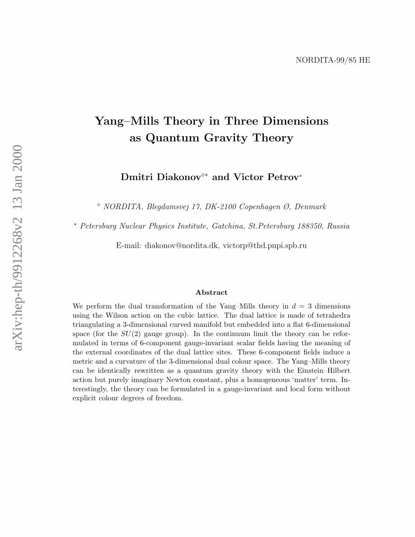
arXiv:hep-th/9912268v2 13 Jan 2000 NORDITA-99/85 HE Yang–Mills Theory in Three Dimensions as Quantum Gravity Theory Dmitri Diakonov ⋄∗ and Victor Petrov ∗ ⋄ NORDITA, Blegdamsvej 17, DK-2100 Copenhagen Ø, Denmark ∗ Petersburg Nuclear Physics Institute, Gatchina, St.Petersburg 188350, Russia E-mail: [email protected], [email protected] Abstract We perform the dual transformation of the Yang–Mills theory in d = 3 dimensions using the Wilson action on the cubic lattice. The dual lattice is made of tetrahedra triangulating a 3-dimensional curved manifold but embedded into a flat 6-dimensional space (for the SU (2) gauge group). In the continuum limit the theory can be refor- mulated in terms of 6-component gauge-invariant scalar fields having the meaning of the external coordinates of the dual lattice sites. These 6-component fields induce a metric and a curvature of the 3-dimensional dual colour space. The Yang–Mills theory can be identically rewritten as a quantum gravity theory with the Einstein–Hilbert action but purely imaginary Newton constant, plus a homogeneous ‘matter’ term. In- terestingly, the theory can be formulated in a gauge-invariant and local form without explicit colour degrees of freedom.
-
Upload
independent -
Category
Documents
-
view
0 -
download
0
Transcript of Yang-Mills theory in three dimensions as a quantum gravity theory
arX
iv:h
ep-t
h/99
1226
8v2
13
Jan
2000
NORDITA-99/85 HE
Yang–Mills Theory in Three Dimensions
as Quantum Gravity Theory
Dmitri Diakonov⋄∗ and Victor Petrov∗
⋄ NORDITA, Blegdamsvej 17, DK-2100 Copenhagen Ø, Denmark
∗ Petersburg Nuclear Physics Institute, Gatchina, St.Petersburg 188350, Russia
E-mail: [email protected], [email protected]
Abstract
We perform the dual transformation of the Yang–Mills theory in d = 3 dimensionsusing the Wilson action on the cubic lattice. The dual lattice is made of tetrahedratriangulating a 3-dimensional curved manifold but embedded into a flat 6-dimensionalspace (for the SU(2) gauge group). In the continuum limit the theory can be refor-mulated in terms of 6-component gauge-invariant scalar fields having the meaning ofthe external coordinates of the dual lattice sites. These 6-component fields induce ametric and a curvature of the 3-dimensional dual colour space. The Yang–Mills theorycan be identically rewritten as a quantum gravity theory with the Einstein–Hilbertaction but purely imaginary Newton constant, plus a homogeneous ‘matter’ term. In-terestingly, the theory can be formulated in a gauge-invariant and local form withoutexplicit colour degrees of freedom.
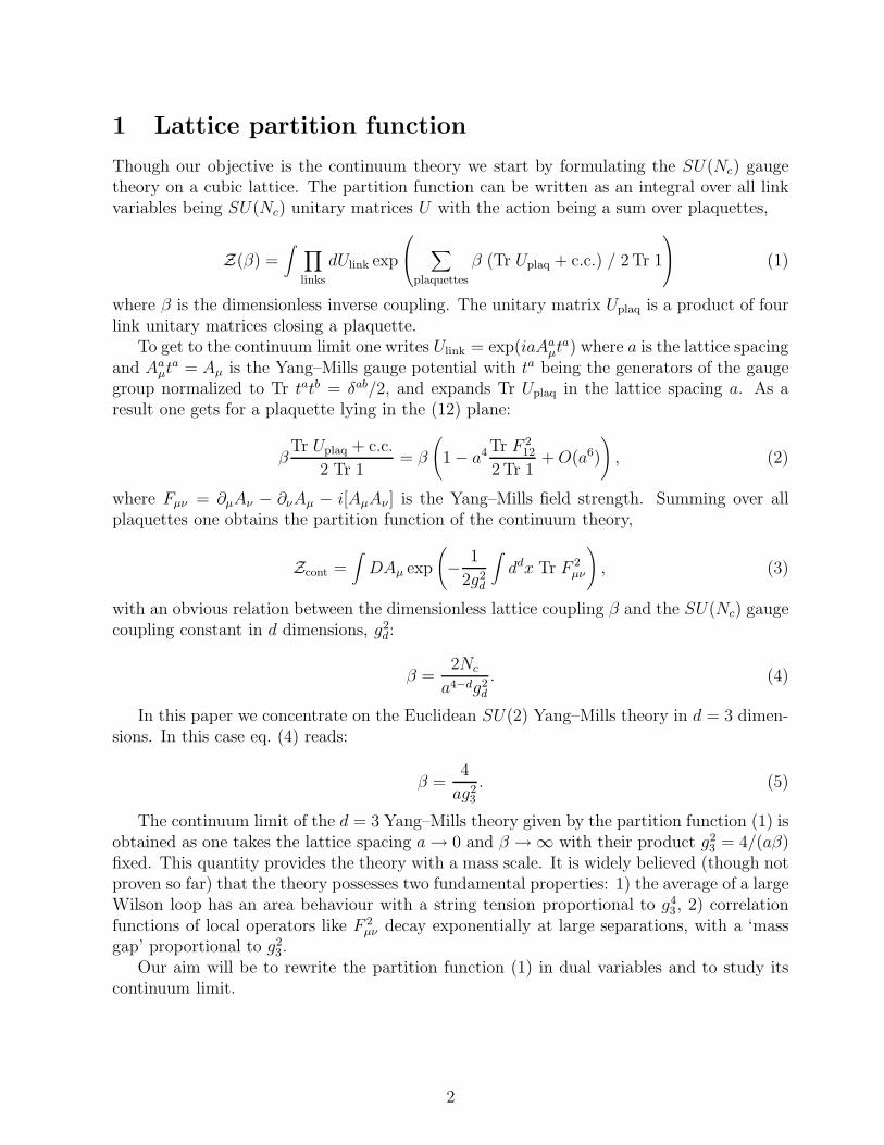
1 Lattice partition function
Though our objective is the continuum theory we start by formulating the SU(Nc) gaugetheory on a cubic lattice. The partition function can be written as an integral over all linkvariables being SU(Nc) unitary matrices U with the action being a sum over plaquettes,
Z(β) =∫
∏
links
dUlink exp
∑
plaquettes
β (Tr Uplaq + c.c.) / 2 Tr 1
(1)
where β is the dimensionless inverse coupling. The unitary matrix Uplaq is a product of fourlink unitary matrices closing a plaquette.
To get to the continuum limit one writes Ulink = exp(iaAaµt
a) where a is the lattice spacingand Aa
µta = Aµ is the Yang–Mills gauge potential with ta being the generators of the gauge
group normalized to Tr tatb = δab/2, and expands Tr Uplaq in the lattice spacing a. As aresult one gets for a plaquette lying in the (12) plane:
βTr Uplaq + c.c.
2 Tr 1= β
(
1 − a4Tr F 212
2 Tr 1+ O(a6)
)
, (2)
where Fµν = ∂µAν − ∂νAµ − i[AµAν ] is the Yang–Mills field strength. Summing over allplaquettes one obtains the partition function of the continuum theory,
Zcont =∫
DAµ exp
(
− 1
2g2d
∫
ddx Tr F 2µν
)
, (3)
with an obvious relation between the dimensionless lattice coupling β and the SU(Nc) gaugecoupling constant in d dimensions, g2
d:
β =2Nc
a4−dg2d
. (4)
In this paper we concentrate on the Euclidean SU(2) Yang–Mills theory in d = 3 dimen-sions. In this case eq. (4) reads:
β =4
ag23
. (5)
The continuum limit of the d = 3 Yang–Mills theory given by the partition function (1) isobtained as one takes the lattice spacing a → 0 and β → ∞ with their product g2
3 = 4/(aβ)fixed. This quantity provides the theory with a mass scale. It is widely believed (though notproven so far) that the theory possesses two fundamental properties: 1) the average of a largeWilson loop has an area behaviour with a string tension proportional to g4
3, 2) correlationfunctions of local operators like F 2
µν decay exponentially at large separations, with a ‘massgap’ proportional to g2
3.Our aim will be to rewrite the partition function (1) in dual variables and to study its
continuum limit.
2
2 Dual transformation
The general idea is to integrate over link variables Ulink in eq. (1) and to make a Fouriertransformation in the plaquette variables Uplaq. This will be made in several steps, one fora subsection.
2.1 Inserting a unity into the partition function
First of all, one needs to introduce explicitly integration over unitary matrices ascribed tothe plaquettes, Uplaq. This is done by inserting a unity for each plaquette into the partitionfunction (1):
1 =∏
plaquettes
∫
dUplaq δ(Uplaq , U1U2U3U4) (6)
where U1...4 are the link variables closing into a given plaquette. The δ-function is understoodwith the group-invariant Haar measure. A realization of such a δ-function is given by WignerD-functions:
δ(U, V ) =∑
J=0, 12,1, 3
2,...
(2J + 1)DJm1m2
(U †)DJm2m1
(V ). (7)
This equation is known as a completeness condition for the D-functions [1]. The mainproperties of the D-functions used in this paper are listed in Appendix A.
Eq. (7) should be understood as follows: if one integrates any function of a unitary matrixU with the r.h.s. of eq. (7) over the Haar measure dU one gets the same function but of theargument V :
∫
dU f(U) δ(U, V ) = f(V ). (8)
Using the multiplication law for the D-functions (see Appendix A, eq. (75)) one can writedown the unity to be inserted for each plaquette in the partition function (1) as
1 =∫
dUplaq
∑
J
(2J + 1) DJm1m2
(U †plaq)D
Jm2m3
(U1)DJm3m4
(U2)DJm4m5
(U3)DJm5m1
(U4) (9)
where U1...4 are the corresponding link variables forming the plaquette under consideration.
2.2 Integrating over plaquette variables
Integrating over plaquette unitary matrices Uplaq becomes now very simple. For each pla-quette of the lattice one has factorized integrals of the type
∫
dUplaq exp
βTr Uplaq + Tr U †
plaq
2 Tr 1
DJm1m2
(U †plaq) = δm1m2
2
βI1(β)TJ(β), (10)
where TJ(β) is the ratio of the modified Bessel functions [2],
3
TJ(β) =I2J+1(β)
I1(β)−→ exp
[
−2J(J + 1)
β
]
at β → ∞. (11)
The quantity TJ(β) is the ‘Fourier transform’ of the Wilson action; since in the latticeformulation the dynamical variables have the meaning of Euler angles and are thereforecompact, the Fourier transform depends on discrete values J = 0, 1/2, 1, 3/2, .... However,as one approaches the continuum limit (β → ∞) the essential values of the plaquette angularmomenta increase as J ∼ √
β and their discreteness becomes less relevant. Strictly speaking,the continuum limit is achieved at plaquette angular momenta J ≫ 1.
We would like to make a side remark on this occasion. The quantity TJ(β) gives theprobability that plaquette momenta J is excited, for given β. For a typical value used inlattice simulations β = 2.6 (in 4 dimensions) we find that the probabilities of having plaquetteexcitations with J = 0, 1/2, 1, 3/2 and 2 are 56%, 29%, 11%, 3% and 1%, respectively. Itmeans that lattice simulations are actually dealing mainly with J = 0, 1/2 and 1 with atiny admixture of higher excitations. It would be important to understand why and howcontinuum physics is reproduced by lattice simulations despite only such small values ofplaquette J ’s are involved.
We get, thus, for the partition function:
Z =
[
2
βI1(β)
]# of plaquettes∑
JP
∏
plaquettes
(2JP + 1) TJP(β)
×∏
links l
∫
dUl DJPm1m2
(U1) DJPm2m3
(U2) DJPm3m4
(U3) DJPm4m1
(U4) (12)
where U1−4 are link variables forming a plaquette with angular momentum JP .
2.3 Integrating over link variables
The difficulty in performing integration over link variables in eq. (12) is due to the factthat any link enters several plaquettes. In d = 2 dimensions every link is shared by twoplaquettes, hence one has to calculate integrals of the type
∫
dUDJ1
kl (U)DJ2
mn(U †) =1
2J1 + 1δJ1J2
δkn δlm (13)
for all links on the lattice. We shall consider this case later, in section 4.In d = 3 dimensions every link is shared by four plaquettes, hence the integral over link
variables is of the type∫
dUDJAm1m2
(U)DJBm3m4
(U)DJCm5m6
(U)DJDm7m8
(U) (14)
where JA,B,C,D are angular momenta associated with four plaquettes intersecting at a givenlink U , and m1−8 are ‘magnetic’ quantum numbers, to be contracted inside closed plaquettes.In d = 4 dimensions there will be six plaquettes intersecting at a given link but we shall notconsider this case here.
4
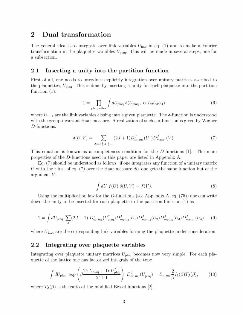
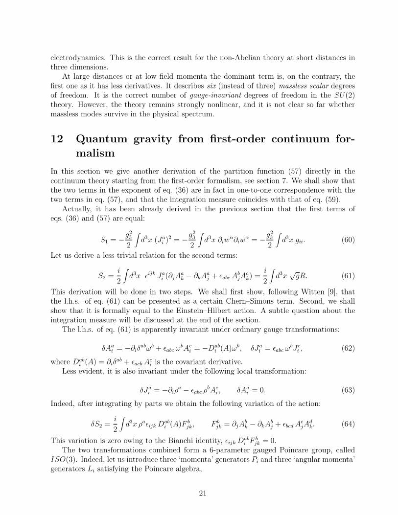
Figure 1: ‘Even’ cubes in checker board order.
The general strategy in calculating the link integrals (14) is (i) to divide by a certain rulefour D-functions into two pairs and to decompose the pairs of D-functions in terms of singleD-functions using eq. (82) of Appendix A, (ii) to integrate the resulting two D-functionsusing eq. (13) and, finally, (iii) to contract the ‘magnetic’ indices. Since all ‘magnetic’ indiceswill be eventually contracted we shall arrive to the partition function written in terms of theinvariant 3nj symbols.
There are several different tactics how to divide four D-functions into two pairs, even-tually leading to anything from 6j to 18j symbols. In this paper we take a route used inrefs.[3, 4], leading to a product of many 6j symbols, although on this route one looses certainsymmetries, and that causes difficulties later on. The gain, however, is that it is more easyto work with 6j symbols than with 12j or 18j symbols. Since important sign factors havebeen omitted in refs.[3, 4] and only final result has been reported there, we feel it necessaryto give a detailed derivation below.
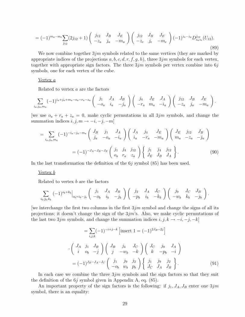
In d = 3 dimensions all plaquettes are shared by two adjacent cubes, therefore, it isnatural to divide all cubes of the lattice into two classes which we shall call ‘even’ and ‘odd’,and to attribute plaquettes only to even cubes. We shall call the cube even if its left-lower-forward corner is a lattice site with even coordinates, (−1)x+y+z = +1. It will be calledodd in the opposite case. The even and odd cubes form a 3-dimensional checker board, asillustrated in Fig.1, where only even cubes are drawn explicitly. The even cubes touch eachother through a common edge or link, as do the odd ones among themselves. The even andodd cubes have common faces or plaquettes. All plaquettes will be attributed to even cubesonly: that is the reason for the division of cubes into two classes.
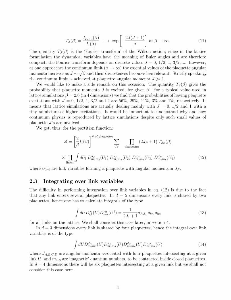
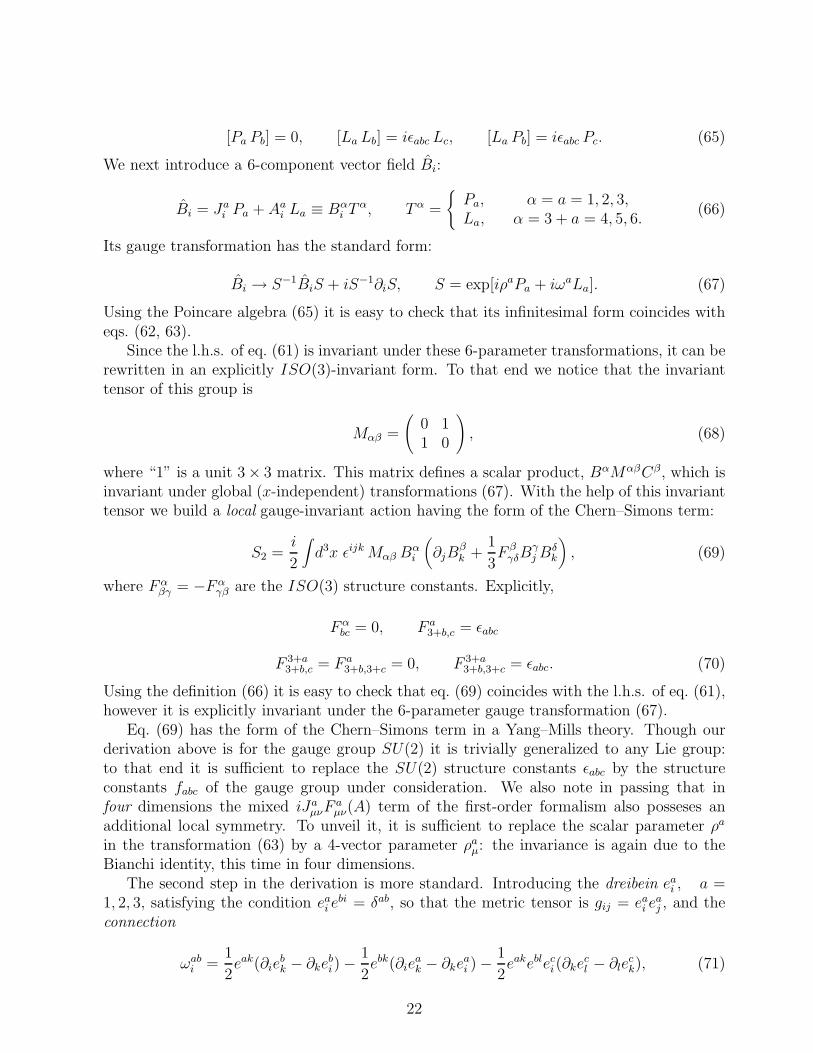
Let us consider an even cube shown in Fig.2.A, B, C, D, E, F denote its 6 faces, numbers from 1 to 12 denote its links or edges,
a, b, c, d, e, f, g, h denote its 8 vertices or sites. Correspondingly, we shall denote plaque-tte angular momenta by JA−F , link variables by U1−12, and the ‘magnetic’ numbers of theD-functions will carry indices a−h referring to the sites the D-functions are connecting.
One can write the traces of products of four D-functions over plaquettes in various ways.To be systematic we shall adhere to the following rule: Link variables in the plaquette are
5
AB
C
DE
F
a
b
c
d
e
f
g
h
1
2
34
5
6
78
9
10
11
12
Figure 2: Elementary even cube
taken in the anti-clock-wise order, as viewed from the center of the even cube to which the
given plaquette belongs. If the link goes in the positive direction of the x, y, z axes we ascribethe U variable to it; otherwise we ascribe the U † variable to it.
With these rules the six plaquettes of the elementary cube shown in Fig.2 bring in thefollowing six traces of the D-function products:
Cube =[
DJAiaib
(U1)DJAibic(U2)D
JAicid
(U †3)D
JAidia(U
†4)] [
DJBjbja
(U †1)D
JBjaje
(U12)DJBjejf
(U5)DJBjf jb
(U †9)]
[
DJC
kckb(U †
2)DJC
kbkf(U9)D
JC
kfkg(U6)D
JC
kgkc(U †
10)] [
DJD
ldlc(U3)DJD
lclg(U10)DJD
lglh(U †
7)DJD
lhld(U †
11)]
[
DJEmema
(U †12)D
JEmamd
(U4)DJEmdmh
(U11)DJEmhme
(U †8)] [
DJFnf ne
(U †5 )DJF
nenh(U8)D
JFnhng
(U7)DJFngnf
(U †6)]
.
(15)Each link variable U1−12 appears in this product twice: once as U , the other time as
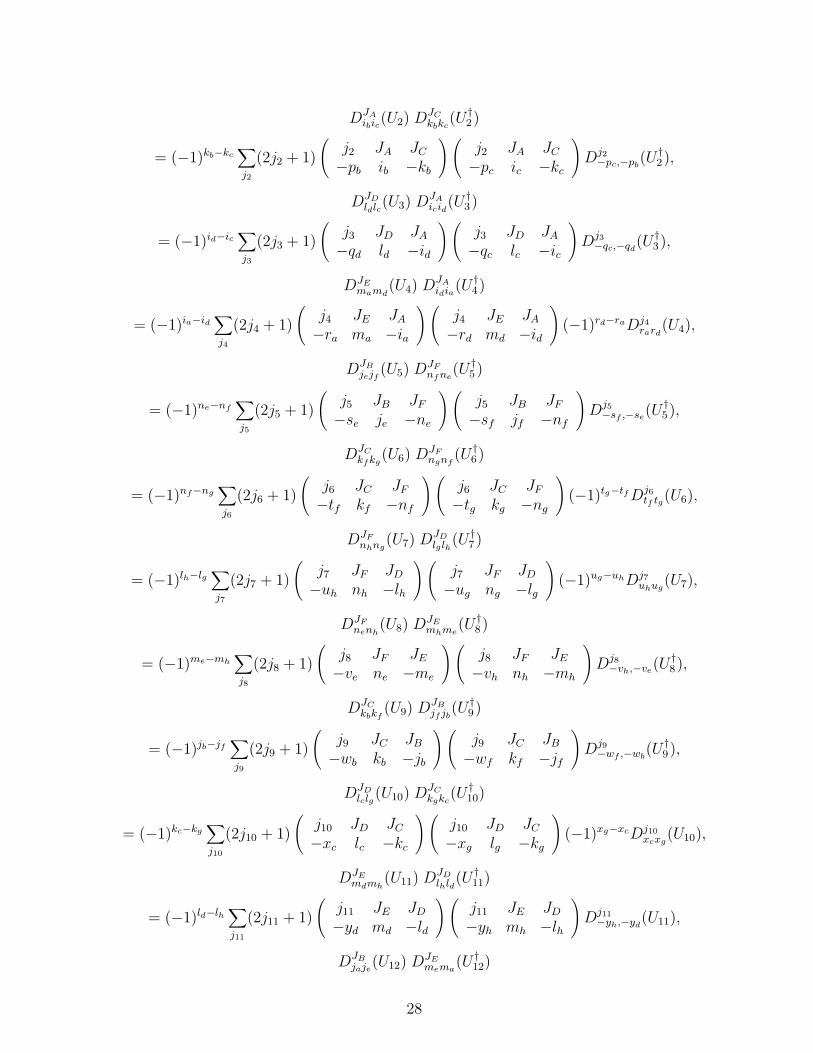
U †. For D(U †) we use eq. (77) of the Appendix A to write it in terms of D(U). Afterthat we can apply the decomposition rule (82) of that Appendix to write down pairs of D-functions in terms of one D-function and two 3jm symbols. The new D-functions correspondto the links and carry angular momenta which we denote by j’s. The 3jm symbols have‘magnetic’ indices which get contracted when all indices related to a given corner of the cubeare assembled together. Though this exercise is straightforward it is rather lengthy, and werelegate it to Appendix B. As a result we get the following expression which is identicallyequal to (15):
Cube =∑
j1...j12
(2j1 + 1)...(2j12 + 1)
Dj1oaob
(U1)Dj2−pc,−pb
(U †2)D
j3−qc,−qd
(U †3)D
j4rard
(U4)Dj5−sf ,−se
(U †5)D
j6tf tg(U6)
Dj7uhug
(U7)Dj8−vh,−ve
(U †8 )Dj9
−wf ,−wb(U †
9 )Dj10xcxg
(U10)Dj11−yh,−yd
(U †11)D
j12zaze
(U12)(
j1 j4 j12
oa ra za
)(
j1 j9 j2
−ob wb pb
)(
j2 j3 j10
pc qc −xc
)(
j4 j3 j11
−rd qd yd
)
(
j12 j8 j5
−ze ve se
)(
j6 j5 j9
−tf sf wf
)(
j6 j10 j7
tg xg ug
)(
j7 j11 j8
−uh yh vh
)
6
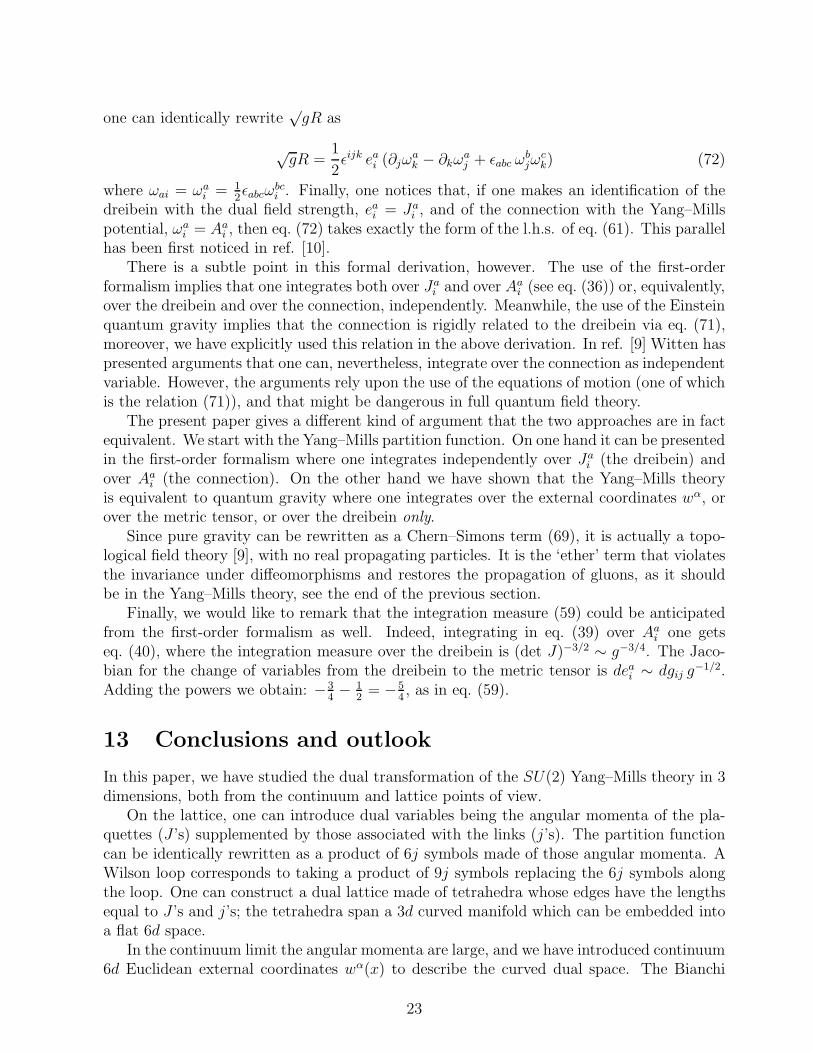
II
III
IV
VVI
I
a
b
c
d
e
f
g
h
12
34
56
78
9
10
11
12
1314
15
1617
18
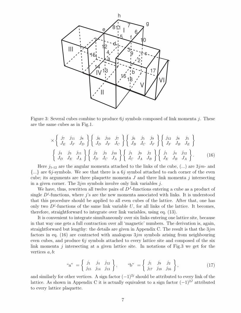
Figure 3: Several cubes combine to produce 6j symbols composed of link momenta j. Theseare the same cubes as in Fig.1.
×
j7 j11 j8
JE JF JD
j6 j10 j7
JD JF JC
j6 j5 j9
JB JC JF
j12 j8 j5
JF JB JE
j4 j3 j11
JD JE JA
j2 j3 j10
JD JC JA
j1 j9 j2
JC JA JB
j1 j4 j12
JE JB JA
. (16)
Here j1−12 are the angular momenta attached to the links of the cube, (...) are 3jm- and... are 6j-symbols. We see that there is a 6j symbol attached to each corner of the evencube; its arguments are three plaquette momenta J and three link momenta j intersectingin a given corner. The 3jm symbols involve only link variables j.
We have, thus, rewritten all twelve pairs of DJ-functions entering a cube as a product ofsingle Dj-functions, where j’s are the new momenta associated with links. It is understoodthat this procedure should be applied to all even cubes of the lattice. After that, one hasonly two Dj-functions of the same link variable U , for all links of the lattice. It becomes,therefore, straightforward to integrate over link variables, using eq. (13).
It is convenient to integrate simultaneously over six links entering one lattice site, becausein that way one gets a full contraction over all ‘magnetic’ numbers. The derivation is, again,straightforward but lengthy: the details are given in Appendix C. The result is that the 3jmfactors in eq. (16) are contracted with analogous 3jm symbols arising from neighbouringeven cubes, and produce 6j symbols attached to every lattice site and composed of the sixlink momenta j intersecting at a given lattice site. In notations of Fig.3 we get for thevertices a, b:
“a” =
j1 j4 j12
j15 j14 j13
, “b” =
j1 j9 j2
j17 j18 j16
, (17)
and similarly for other vertices. A sign factor (−1)2j should be attributed to every link of thelattice. As shown in Appendix C it is actually equivalent to a sign factor (−1)2J attributedto every lattice plaquette.
7
3 Lattice partition function as a product of 6j symbols
We summarize here the recipe derived in the previous section. One first divides all 3-cubesinto two classes, even and odd ones. They form a 3-dimensional checker board depicted inFig.1. All even cubes are characterized by their plaquette momenta J . The edges of evencubes have link momenta j; each link is shared by two even cubes.
To each of the eight corners of an even cube one attributes a 6j symbol of the type
j1 j2 j3
JA JB JC
(18)
where J ’s are plaquette and j’s are link momenta intersecting in a given corner of a cube.The rule is that link 1 is perpendicular to plaquette A, link 2 is perpendicular to plaquetteB and link 3 is perpendicular to plaquette C. Four triades, (j1JBJC), (j2JAJC), (j3JAJB)and (j1j2j3) satisfy triangle inequalities.
To each lattice site one attributes a 6j symbol of the type
j1 j2 j3
j4 j5 j6
(19)
where j’s are the six link momenta entering a given lattice site. The rule is that link 4 isa continuation of link 1 lying in the same direction, link 5 is a continuation of link 2 andlink 6 is a continuation of link 3. Four triades, (j1j2j3), (j1j5j6), (j2j4j6) and (j3j4j5) satisfytriangle inequalities.
Actually, each lattice site has five 6j symbols ascribed to it: four are originating fromthe corners of the even cubes adjacent to the site and are of the type (18), and one is of thetype (19).
The lattice partition function (1) or (12) can be identically rewritten as a product of the6j symbols described above. Independent summation over all possible plaquette momenta Jand all possible link momenta j is understood. We write the partition function in a symbolicform:
Z =
[
2
βI1(β)
]# of plaquettes∑
JP , jl
∏
plaquettes
(2JP + 1) TJP(β) (−1)2JP
∏
links
(2jl + 1)
×∏
even cubes corners
j j jJ J J
∏
lattice sites
j j jj j j
. (20)
The plaquette weights TJ(β) are given by eq. (11). Apart from the sign factor essentially thesame expression was given in refs. [3, 4] 1. The sign factor is equal to ±1 if the total numberof half-integer plaquettes J ’s is even (odd). Since plaquettes with half-integer momenta formclosed surfaces it may seem that the sign factor can be omitted. In a general case, however,when one consideres vacuum averages of operators this is not so, therefore, it is preferableto keep the sign factor.
1We are grateful to P.Pobylitsa who has independently derived eq. (20).
8
4 Simple example: d = 2 Yang–Mills
In a simple exactly soluble case of the 2-dimensional SU(2) theory every link is shared byonly two plaquettes. Therefore, the link integration is of the type given by eq. (13): itrequires that all plaquettes on the lattice have identical momenta J . The partition functionthus becomes a single sum over the common J :
Z =
[
2
βI1(β)
]# of plaquettes∑
J
[TJ(β)]# of plaquettes , (21)
the number of plaquettes being equal to V/a2 where V is the full lattice volume (full areain this case) and a is the lattice spacing.
A slightly less trivial exercise is to compute the average of the Wilson loop. Let theWilson loop be in the representation js. It means that one inserts Djs(U) for all linksalong the loop. One gets therefore integrals of two D-functions outside and inside the loop,and integrals of three D-functions for links along the loop. The first integral says that allplaquettes outside the loop are equal to a common J . The second integral says that allplaquettes inside the loop are equal to a common J ′. Integrals along the loop require thatJ, J ′ and js satisfy the triangle inequality. We have thus for the average of the Wilson loopof area S:
〈Wjs(S)〉 =
∑
J [TJ(β)]V
a2∑J+js
J ′=|J−js|[TJ ′(β) / TJ(β)]
S
a2
∑
J [TJ(β)]V
a2
. (22)
This is an exact expression for the lattice Wilson loop, however we wish to explore itscontinuum limit. It implies that V/a2 → ∞, S/a2 → ∞ but S ≪ V ; β → ∞, a → 0 butβa2 = 4/g2
2 fixed, where g22 is the physical coupling constant having the dimension of mass2,
see eq. (4).We take V/a2 → ∞ first of all, which requires that only the J = 0 term contributes to
the sum, with T0(β) ≡ 1; consequently all momenta inside the loop are that of the source,J ′ = js. Taking into account the asymptotics (11) of TJ(β) at large β we obtain
〈Wjs(S)〉 = [Tjs
(β)]S
a2 = exp
[
−g22
2js(js + 1) S
]
(23)
which is, of course, the well-known area behaviour of the Wilson loop with the string tensionproportional to the Casimir eigenvalue.
5 Dual lattice: tetrahedra and octahedra
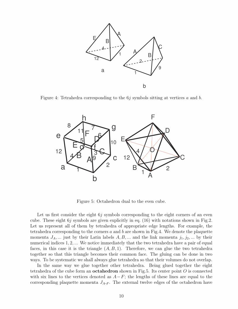
We now turn to the construction of the dual lattice.Each 6j symbol of the exact partition function (20) encodes four triangle inequalities
between the plaquette J ’s and the link j’s. It is therefore natural to represent all 6j symbolsby tetrahedra whose six edges have lengths equal to the six momenta of a given 6j symbol.Four faces of a tetrahedron form four triangles, so that the triangle inequalities for themomenta are satisfied automatically.
9
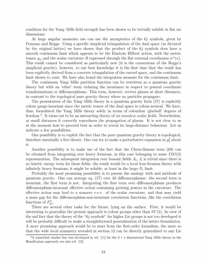
A
BE
AB
C
a
b
1
4
12
1
2
9
Figure 4: Tetrahedra corresponding to the 6j symbols sitting at vertices a and b.
AB
C
DE
F
a
b
c
d
e
f
gh
12
34
56
78
9
10
11
12
A
E
B
C
D
F
12
124 O
Figure 5: Octahedron dual to the even cube.
Let us first consider the eight 6j symbols corresponding to the eight corners of an evencube. These eight 6j symbols are given explicitly in eq. (16) with notations shown in Fig.2.Let us represent all of them by tetrahedra of appropriate edge lengths. For example, thetetrahedra corresponding to the corners a and b are shown in Fig.4. We denote the plaquettemomenta JA, ... just by their Latin labels A, B, ... and the link momenta j1, j2, ... by theirnumerical indices 1, 2, ... We notice immediately that the two tetrahedra have a pair of equalfaces, in this case it is the triangle (A, B, 1). Therefore, we can glue the two tetrahedratogether so that this triangle becomes their common face. The gluing can be done in twoways. To be systematic we shall always glue tetrahedra so that their volumes do not overlap.
In the same way we glue together other tetrahedra. Being glued together the eighttetrahedra of the cube form an octahedron shown in Fig.5. Its center point O is connectedwith six lines to the vertices denoted as A−F ; the lengths of these lines are equal to thecorresponding plaquette momenta JA−F . The external twelve edges of the octahedron have
10
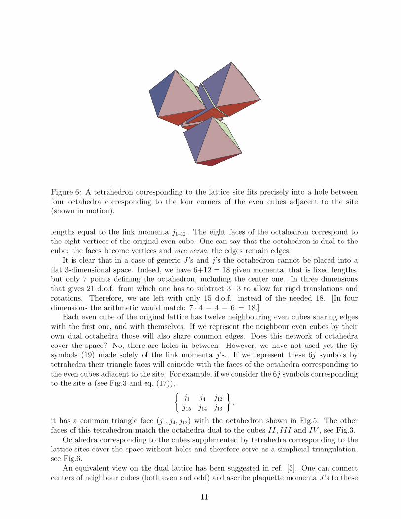
Figure 6: A tetrahedron corresponding to the lattice site fits precisely into a hole betweenfour octahedra corresponding to the four corners of the even cubes adjacent to the site(shown in motion).
lengths equal to the link momenta j1−12. The eight faces of the octahedron correspond tothe eight vertices of the original even cube. One can say that the octahedron is dual to thecube: the faces become vertices and vice versa; the edges remain edges.
It is clear that in a case of generic J ’s and j’s the octahedron cannot be placed into aflat 3-dimensional space. Indeed, we have 6+12 = 18 given momenta, that is fixed lengths,but only 7 points defining the octahedron, including the center one. In three dimensionsthat gives 21 d.o.f. from which one has to subtract 3+3 to allow for rigid translations androtations. Therefore, we are left with only 15 d.o.f. instead of the needed 18. [In fourdimensions the arithmetic would match: 7 · 4 − 4 − 6 = 18.]
Each even cube of the original lattice has twelve neighbouring even cubes sharing edgeswith the first one, and with themselves. If we represent the neighbour even cubes by theirown dual octahedra those will also share common edges. Does this network of octahedracover the space? No, there are holes in between. However, we have not used yet the 6jsymbols (19) made solely of the link momenta j’s. If we represent these 6j symbols bytetrahedra their triangle faces will coincide with the faces of the octahedra corresponding tothe even cubes adjacent to the site. For example, if we consider the 6j symbols correspondingto the site a (see Fig.3 and eq. (17)),
j1 j4 j12
j15 j14 j13
,
it has a common triangle face (j1, j4, j12) with the octahedron shown in Fig.5. The otherfaces of this tetrahedron match the octahedra dual to the cubes II, III and IV , see Fig.3.
Octahedra corresponding to the cubes supplemented by tetrahedra corresponding to thelattice sites cover the space without holes and therefore serve as a simplicial triangulation,see Fig.6.
An equivalent view on the dual lattice has been suggested in ref. [3]. One can connectcenters of neighbour cubes (both even and odd) and ascribe plaquette momenta J ’s to these
11
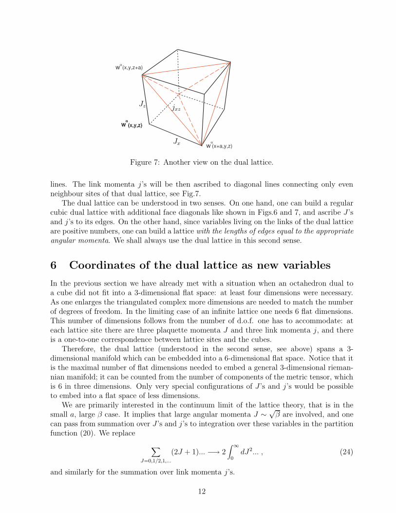
α
w (x,y,z)α
w (x,y,z)α
w (x,y,z)
w (x,y,z+a)α
α
(x+a,y,z)w
Jz
Jx
jxz
Figure 7: Another view on the dual lattice.
lines. The link momenta j’s will be then ascribed to diagonal lines connecting only evenneighbour sites of that dual lattice, see Fig.7.
The dual lattice can be understood in two senses. On one hand, one can build a regularcubic dual lattice with additional face diagonals like shown in Figs.6 and 7, and ascribe J ’sand j’s to its edges. On the other hand, since variables living on the links of the dual latticeare positive numbers, one can build a lattice with the lengths of edges equal to the appropriate
angular momenta. We shall always use the dual lattice in this second sense.
6 Coordinates of the dual lattice as new variables
In the previous section we have already met with a situation when an octahedron dual toa cube did not fit into a 3-dimensional flat space: at least four dimensions were necessary.As one enlarges the triangulated complex more dimensions are needed to match the numberof degrees of freedom. In the limiting case of an infinite lattice one needs 6 flat dimensions.This number of dimensions follows from the number of d.o.f. one has to accommodate: ateach lattice site there are three plaquette momenta J and three link momenta j, and thereis a one-to-one correspondence between lattice sites and the cubes.
Therefore, the dual lattice (understood in the second sense, see above) spans a 3-dimensional manifold which can be embedded into a 6-dimensional flat space. Notice that itis the maximal number of flat dimensions needed to embed a general 3-dimensional rieman-nian manifold; it can be counted from the number of components of the metric tensor, whichis 6 in three dimensions. Only very special configurations of J ’s and j’s would be possibleto embed into a flat space of less dimensions.
We are primarily interested in the continuum limit of the lattice theory, that is in thesmall a, large β case. It implies that large angular momenta J ∼
√β are involved, and one
can pass from summation over J ’s and j’s to integration over these variables in the partitionfunction (20). We replace
∑
J=0,1/2,1,...
(2J + 1)... −→ 2∫ ∞
0dJ2... , (24)
and similarly for the summation over link momenta j’s.
12
The next step is to ascribe a 6-dimensional Lorentz scalar field wα(x), α = 1, ..., 6 tothe centers of all cubes of the original lattice, see Fig.7. We shall call them coordinatesof the dual lattice. They are scalars because in three dimensions the cubes are scalars.The argument of the six-component scalar field is the coordinate of the center of the cubein question, however, we shall consider wα(x) as continuous functions. Since six functionsdepend only on three coordinates there are three relations between wα(x) at any point; theserelations define a curved 3-dimensional manifold whose triangulation is given by the set ofJ ’s and j’s.
We next define six-dimensional angular momenta as differences of wα(x) taken at thecenters of neighbour cubes:
Jαx
(
x +a
2, y, z
)
= wα(x + a, y, z) − wα(x, y, z) = a∂xwα +
a2
2∂2
xwα + ... ,
jαxz
(
x +a
2, y, z +
a
2
)
= wα(x + a, y, z) − wα(x, y, z + a)=a(∂x − ∂z)wα + O(a2), (25)
and so on. The lengths of these 6-vectors are, by construction, the lengths of the edges ofthe dual lattice.
The six functions wα(x) can be called external coordinates of the manifold; they inducea metric tensor of the manifold determined by
gij(x) = ∂iwα∂jw
α. (26)
As usual in differential geometry one can define the Christoffel symbol,
Γi,jk(x) =1
2(∂jgik + ∂kgij − ∂igjk) = ∂iw
α∂j∂kwα ≡ (wi · wjk), (27)
and the Riemann tensor,
Rijkl(x) =1
2(∂j∂kgil + ∂i∂lgjk − ∂j∂lgik − ∂i∂kgjl) + Γm,jkΓ
mil − Γm,jlΓ
mik
= [(wik · wjl) − gpq(wp · wik) (wq · wjl] − [k ↔ l]. (28)
The contravariant tensor is inverse to the covariant one,
gijgjk = δik, (29)
and can be used to rise indices, and for contractions. The determinant of the metric tensoris
g = det gij =1
3!ǫijk ǫlmn(wi · wl) (wj · wm) (wk · wn), (30)
and the contravariant metric tensor is
gij =1
2gǫiklǫjmn(wk · wm) (wl · wn). (31)
There is a useful identity for the antisymmetrized product of two contravariant tensors, validin 3 dimensions:
13

gikgjl − gilgjk = ǫijm ǫkln gmn / g. (32)
The scalar curvature is obtained as a full contraction:
R = gik gjl Rijkl =1
2(gik gjl − gil gjk) Rijkl
=1
2g2ǫijkǫi′j′k′
(wk ·wk′)[2g (wii′ ·wjj′)−ǫplmǫql′m′
(wp ·wii′)(wq ·wjj′)(wl ·wl′)(wm ·wm′)]. (33)
Recalling that wα is a 6-dimensional vector we can rewrite the scalar curvature in anotherform:
R =1
72 g2ǫαβγδεη ǫα′β′γ′δ′εη ǫijk ǫi′j′k′
ǫpll′ǫqmm′
wαi wα′
i′ wβj wβ′
j′ wγkwγ′
k′wδlmwδ′
l′m′wζpw
ζq . (34)
This form makes it clear that the scalar curvature is zero if wα has only three nonzerocomponents, which corresponds to a flat 3-dimensional manifold.
Finally, we would like to point out the Jacobian for the change of integration variablesfrom the set of the lengths of the tetrahedra edges, J2
i and j2i given at all lattice sites, to the
external coordinates wα. In the continuum limit this Jacobian is quite simple. It is given bythe determinant of a 6 × 6 matrix composed of the second derivatives:
∏
x
dJ2i (x) dj2
i (x) =∏
x
dwα(x) Jac(w), Jac(w) = det wαij. (35)
Since wαij = wα
ji there are actually six independent second derivatives. The Jacobian is zeroin the degenerate case when the triangulation by tetrahedra can be embedded in less than6 dimensions.
7 Continuum duality transformation and Bianchi iden-
tity
It is instructive at this point to compare the duality transformation on the lattice with thatin the continuum theory. The continuum partition function (3) can be written with the helpof an additional gaussian integration over the ‘dual field strength’, Ja
ij :
Z =∫
DJaij DAa
i exp∫
d3x
[
−g23
4J2
ij +i
2Ja
ij(∂iAaj − ∂jA
ai + ǫabcAb
iAcj)
]
. (36)
Eq. (36) is usually called the first-order formalism.In the Abelian case when the Ai commutator term is absent, integration over Ai results
in the δ-function of the Bianchi identity,
∂iJij = 0, or ǫijk∂iJk = 0, Jk =1
2ǫijkJij. (37)
Because of this identity, one can parametrize Jk = ∂kw, and get for the partition function:
14
Zabel =∫
Dw exp∫
d3x
[
−g23
2(∂kw)2
]
. (38)
It represents a theory of a free massless scalar field w. It is in accordance with that in a 3dAbelian theory there is only one physical (transverse) polarization. It is easy to check thatgauge-invariant correlation functions of field strengths coincide with those computed in theoriginal formulation.
In the non-Abelian case integration in Aai is more complicated, and there is no simple
Bianchi identity for Jak = (1/2)ǫijkJ
aij . However, one can formally perform the Gaussian
integration over Aai [5] resulting in:
Z =∫
DJai det
1
2 (J −1) exp∫
d3x
[
−g23
2(Ja
i )2 − i
2(ǫijm∂jJ
am) (J −1)ab
ik (ǫkln∂lJbn)
]
(39)
where J −1 is the inverse matrix,
(J −1)abik ǫbcdǫklmJd
m = δacδil; det(J −1) = (det Jak )−3. (40)
Notice that the second term in the exponent is purely imaginary; the full partition functionis real because for each configuration Ja
i (x) there exists a configuration with −Jai (x), which
adds a complex conjugate expression.We now turn to the discretized version of the dual theory. As explained above, we
need 6 flat dimensions to embed the dual lattice, and we have introduced 6-dimensionalmomenta Jα, see eq. (25). These momenta apparently satisfy, e.g., the identity (see Fig.7for notations):
Jαz
(
x, y, z +a
2
)
− Jαx
(
x +a
2, y, z
)
= wα(x, y, z + a) − wα(x + a, y, z)
= Jαz
(
x + a, y, z +a
2
)
− Jαx
(
x +a
2, y, z + a
)
, (41)
and similarly for other components. This is nothing but a discretized version of the Bianchiidentity,
ǫijk∂iJαk = 0, α = 1, ..., 6. (42)
Therefore, in 6 dimensions one recovers the simple (flat) form of the Bianchi identity forthe dual field strength. One can say that the complicated (nonlinear) form of the usualnon-Abelian Bianchi identity is a result of the projection of the flat Bianchi identity ontothe curved colour space.
8 Wilson loop
In this section we present the Wilson loop in the representation js,
Wjs=
1
2js + 1Tr P exp i
∮
dxiAai T
a, (43)
15
in terms of dual variables.In terms of the original lattice the Wilson loop corresponds to adding a product of the
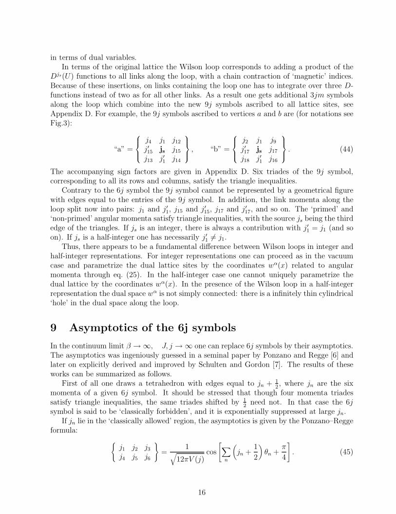
Djs(U) functions to all links along the loop, with a chain contraction of ‘magnetic’ indices.Because of these insertions, on links containing the loop one has to integrate over three D-functions instead of two as for all other links. As a result one gets additional 3jm symbolsalong the loop which combine into the new 9j symbols ascribed to all lattice sites, seeAppendix D. For example, the 9j symbols ascribed to vertices a and b are (for notations seeFig.3):
“a” =
j4 j1 j12
j′15 js j15
j13 j′1 j14
, “b” =
j2 j1 j9
j′17 js j17
j18 j′1 j16
. (44)
The accompanying sign factors are given in Appendix D. Six triades of the 9j symbol,corresponding to all its rows and columns, satisfy the triangle inequalities.
Contrary to the 6j symbol the 9j symbol cannot be represented by a geometrical figurewith edges equal to the entries of the 9j symbol. In addition, the link momenta along theloop split now into pairs: j1 and j′1, j15 and j′15, j17 and j′17, and so on. The ‘primed’ and‘non-primed’ angular momenta satisfy triangle inequalities, with the source js being the thirdedge of the triangles. If js is an integer, there is always a contribution with j′1 = j1 (and soon). If js is a half-integer one has necessarily j′1 6= j1.
Thus, there appears to be a fundamental difference between Wilson loops in integer andhalf-integer representations. For integer representations one can proceed as in the vacuumcase and parametrize the dual lattice sites by the coordinates wα(x) related to angularmomenta through eq. (25). In the half-integer case one cannot uniquely parametrize thedual lattice by the coordinates wα(x). In the presence of the Wilson loop in a half-integerrepresentation the dual space wα is not simply connected: there is a infinitely thin cylindrical‘hole’ in the dual space along the loop.
9 Asymptotics of the 6j symbols
In the continuum limit β → ∞, J, j → ∞ one can replace 6j symbols by their asymptotics.The asymptotics was ingeniously guessed in a seminal paper by Ponzano and Regge [6] andlater on explicitly derived and improved by Schulten and Gordon [7]. The results of theseworks can be summarized as follows.
First of all one draws a tetrahedron with edges equal to jn + 12, where jn are the six
momenta of a given 6j symbol. It should be stressed that though four momenta triadessatisfy triangle inequalities, the same triades shifted by 1
2need not. In that case the 6j
symbol is said to be ‘classically forbidden’, and it is exponentially suppressed at large jn.If jn lie in the ‘classically allowed’ region, the asymptotics is given by the Ponzano–Regge
formula:
j1 j2 j3
j4 j5 j6
=1
√
12πV (j)cos
[
∑
n
(
jn +1
2
)
θn +π
4
]
. (45)
16
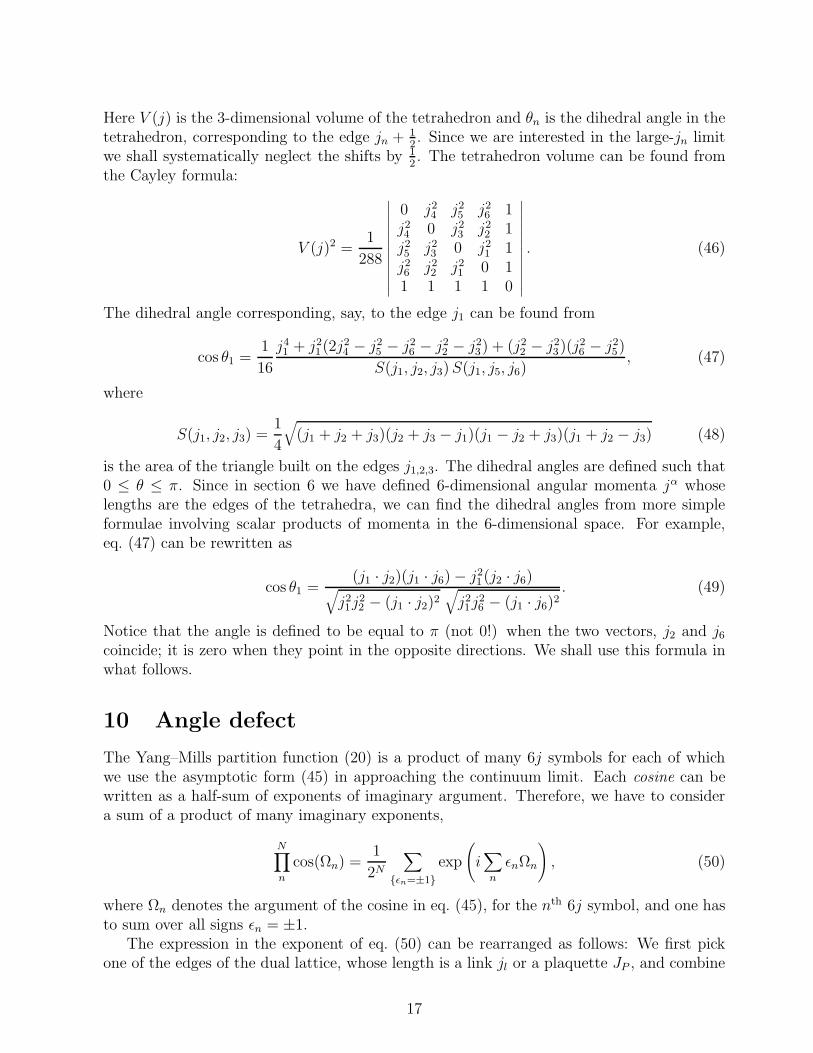
Here V (j) is the 3-dimensional volume of the tetrahedron and θn is the dihedral angle in thetetrahedron, corresponding to the edge jn + 1
2. Since we are interested in the large-jn limit
we shall systematically neglect the shifts by 12. The tetrahedron volume can be found from
the Cayley formula:
V (j)2 =1
288
∣
∣
∣
∣
∣
∣
∣
∣
∣
∣
∣
∣
0 j24 j2
5 j26 1
j24 0 j2
3 j22 1
j25 j2
3 0 j21 1
j26 j2
2 j21 0 1
1 1 1 1 0
∣
∣
∣
∣
∣
∣
∣
∣
∣
∣
∣
∣
. (46)
The dihedral angle corresponding, say, to the edge j1 can be found from
cos θ1 =1
16
j41 + j2
1(2j24 − j2
5 − j26 − j2
2 − j23) + (j2
2 − j23)(j
26 − j2
5)
S(j1, j2, j3) S(j1, j5, j6), (47)
where
S(j1, j2, j3) =1
4
√
(j1 + j2 + j3)(j2 + j3 − j1)(j1 − j2 + j3)(j1 + j2 − j3) (48)
is the area of the triangle built on the edges j1,2,3. The dihedral angles are defined such that0 ≤ θ ≤ π. Since in section 6 we have defined 6-dimensional angular momenta jα whoselengths are the edges of the tetrahedra, we can find the dihedral angles from more simpleformulae involving scalar products of momenta in the 6-dimensional space. For example,eq. (47) can be rewritten as
cos θ1 =(j1 · j2)(j1 · j6) − j2
1(j2 · j6)√
j21j
22 − (j1 · j2)2
√
j21j
26 − (j1 · j6)2
. (49)
Notice that the angle is defined to be equal to π (not 0!) when the two vectors, j2 and j6
coincide; it is zero when they point in the opposite directions. We shall use this formula inwhat follows.
10 Angle defect
The Yang–Mills partition function (20) is a product of many 6j symbols for each of whichwe use the asymptotic form (45) in approaching the continuum limit. Each cosine can bewritten as a half-sum of exponents of imaginary argument. Therefore, we have to considera sum of a product of many imaginary exponents,
N∏
n
cos(Ωn) =1
2N
∑
ǫn=±1
exp
(
i∑
n
ǫnΩn
)
, (50)
where Ωn denotes the argument of the cosine in eq. (45), for the nth 6j symbol, and one hasto sum over all signs ǫn = ±1.
The expression in the exponent of eq. (50) can be rearranged as follows: We first pickone of the edges of the dual lattice, whose length is a link jl or a plaquette JP , and combine
17
all dihedral angles θn related to this edge, as coming from the nth tetrahedron. We then sumover all edges of the dual lattice. Therefore, we can write:
∑
n
ǫnΩn =∑
P
JP
(
4∑
n=1
ǫnθn(JP )
)
+∑
l
jl
(
6∑
n=1
ǫnθn(jl)
)
, ǫn = ±1. (51)
As seen, e.g., from Fig.7, each plaquette J enters four tetrahedra, therefore the correspondingsum over n in eq. (51) goes from 1 to 4. Each link j enters six tetrahedra, therefore in thiscase the sum is over six dihedral angles θn(j), with appropriate signs ǫn.
Let us consider the contribution to eq. (50) when all signs ǫn = +1, and let us for amoment assume that the dual lattice spans a 3-dimensional Euclidean manifold. The sumof the dihedral angles about an edge is then equal to 4π − 2π = 2π in case of summing overfour tetrahedra, and equal to 6π − 2π = 4π in case of summing over six tetrahedra. In thefirst case we get exp(2πiJ) = (−1)2J ; in the second case we get exp(4πij) = (−1)4j = +1.Notice that the sign factor (−1)2J compensates exactly the same factor in the partitionfunction (20). We conclude that, if the configuration of the momenta is ‘flat’, there exists acontribution to the sum (50) that does not oscillate with varying J ’s and j’s. In fact, thereare exactly two such contributions corresponding to taking all signs ǫn = ±1 simultaneously.Contributions of any other choice of the signs are oscillating fast at large J ’s and j’s, andthus die out in the continuum limit.
A generic configuration of momenta cannot be embedded into a flat 3-dimensional space,however. Therefore, the sum of dihedral angles about the edges J and j will, generally, differfrom 2π and 4π, respectively. These differences are sometimes called angle deficiencies orangle defects (we shall use the second term). Let us denote them:
Θ(J) =4∑
n=1
θn(J) − 2π, (52)
Θ(j) =6∑
n=1
θn(j) − 4π. (53)
Our task is to point out contributions to eq. (50) that survive the continuum limit in ageneral case when the dual lattice is a curved 3-dimensional manifold. To be more precise,we have to consider the sum of all momenta on the lattice times their angle defects,
exp i
[
∑
P
JP Θ(JP ) +∑
l
jlΘ(jl)
]
, (54)
and to find the contribution of the order of a3 to this exponent, where a is the latticespacing. The O(a3) order is needed to compensate for the 1/a3 factor arising as one goesfrom summation over the lattice points to integration over the 3-dimensional space.
In the continuum limit we assume that the momenta are given by the gradients of a 6-component function wα(x) having the meaning of the 6-dimensional coordinates of the duallattice sites, see eq. (25). If we restrict ourselves to the first terms in the gradient expansionin eq. (25), the momenta will be expressed only through three vectors, ∂xw
α, ∂ywα and
∂zwα. Three vectors define a flat 3-dimensional space; therefore, the angle defects Θ are
18
zero in the first-derivative approximation. To get a non-zero angle defect it is necessary toexpand the momenta in eq. (25) up to the second derivatives of wα. We shall see that it isalso sufficient in three dimensions.
Since the angle defects Θ’s vanish if j’s are taken to the first approximation of the gradientexpansion, it means that the expansion of Θ’s starts from terms linear in the lattice spacinga. According to eq. (25) the expansion of the momenta also starts from terms linear ina. Therefore, one can expect that the expansion of the exponent in eq. (54) starts fromthe O(a2) terms. Were that so, the configuration would be too ‘ultraviolet’ and would notsurvive the continuum limit. Fortunately, there appears to be an exact cancellation of allO(a2) terms in the sum over several neighbour edges of the dual lattice, so that the exponentin eq. (54) proves to be finite in the continuum limit.
We next embark a rather tedious enterprise of calculating the angle defects about sixplaquette J ’s in a cube (each entering four tetrahedra), and about twelve link j’s beingedges of that cube (each involved in six tetrahedra, see section 5). Unluckily, it seems thatit is the minimal elementary group that is being repeated through the lattice. It meansthat we have to compute as much as 6 · 4 + 12 · 6 = 96 dihedral angles, expressing themthrough the first and second gradients of the 6-component function wα using eqs. (25, 49).This formidable calculation has been performed by heavily exploiting Mathematica. Theintermediate results are very lengthy and we do not present them here. However, the finalresult is beautiful. From a direct calculation we obtain:
exp i
[
∑
P
JP Θ(JP ) +∑
l
jlΘ(jl)
]
= exp i∑
points x
a3 1
2
√
g(w) R(w)
= expi
2
∫
d3x√
g(w) R(w), (55)
where g is the determinant of the induced metric tensor as given by eq. (30), and R is thecorresponding scalar curvature given by eq. (33). Actually, we obtain the expression for thel.h.s. of eq. (55) in the form of eq. (33) (written in components, 384 terms!) from where werecognize that we are dealing with the scalar curvature.
In fact this result is a concrete realization of a more general theory developed many yearsago by Regge [6, 8]. In these papers it was shown that the l.h.s. of eq. (55) should be equalto its r.h.s. for any simplicial triangulation, provided it has a smooth continuum limit. Norelation of the scalar curvature R to any concrete triangulation was given, though. We feelthat it is the first time that this ingenious relation has been derived explicitly for a concretetriangulation, and the continuum limit shown to exist.
11 Full partition function
Having dealt with the 6j symbols of the partition function (20) we now turn to the weightfactors TJ(β). According to eq. (11) at large β and J we have:
∏
plaquettes
TJ(β) = exp
−∑
plaquettes
2J2
β
19

= exp
[
−∫
d3x
a3
2 J2i
β
]
= exp
[
−∫
d3xg23
2∂iw
α∂iwα + O(a2)
]
, (56)
where the relation (5) between β and the physical coupling constant g23 has been used,
together with the gradient expansion for the angular momenta (25). Combining eqs. (55,56) and using ∂iw
α∂iwα = gii(w) we get finally for the Yang–Mills partition function:
Z =∫
Dwα(x) Jac(w) g(w)−5
4 exp∫
d3x
[
−g23
2gii +
i
2
√g R
]
. (57)
The second term is the Einstein–Hilbert action with a purely imaginary Newton constant;it is invariant under global 6-dimensional rotations of the external coordinates wα(x) and,more important, under local 3-dimensional diffeomorphisms wα(x) → wα(x′(x)).
The first term in eq. (57) can be viewed as a ‘matter’ source,
− g23
2
∫
d3x gii = −g23
2
∫
d3x√
g T ijgij , (58)
with the stress-energy tensor T ij√
g = δij violating the invariance under diffeomorphisms.Since it is homogeneous in space it can be called the ‘ether’.
The functional measure in eq. (57) arises from two sources. One factor is the Jacobianfor the change of variables from the tetrahedra edges J ’s and j’s to wα, see eq. (35). Theother factor arises from the tetrahedra volumes in the asymptotics of the 6j symbols (45).In the continuum limit the tetrahedron volume can be written as V (j) ∼ √
g, and there are5 tetrahedra per lattice site, see section 3.
Once the partition function is written in covariant terms one can forget the origin ofthe external coordinates wα (as the coordinates of the dual lattice) and consider the metrictensor gij as independent dynamical variables over which one integrates in eq. (57). TheJacobian for this change of variables can be easily worked out: in fact it is the inverse ofJac(w) introduced in eq. (35). As a result we get the integration measure for the partitionfunction (57):
∫
Dgij g− 5
4 , instead of∫
Dgij g−2, (59)
which would be the invariant measure in 3d. We shall get an independent check of the power−5
4in the next section. However, it is anyhow a local counterterm not affecting the physics.We stress that the partition function written in terms of the metric tensor does not
contain explicit colour degrees of freedom. Nevertheless, implicitly the theory doescontain three gluons at short distances.
Indeed, let us make a simple dimensional analysis of eq. (57). The dimension of the firstterm in eq. (57) is g2
3∂2w2 (we are just counting the number of derivatives and the overall
power of w); the dimension of the second term is ∂3w1. At short distances where quantumfluctuations of wα(x) vary fast, the second term dominates the first one. Meanwhile, thesecond term is a fast-oscillating functional at nonzero R. Therefore, the leading contributionto the functional integral arises from zero-curvature fluctuations of wα, that is essentiallyfrom the 3-dimensional wα. Being plugged into the first term, the three components ofwα describe three massless scalar fields. These fields correspond to three gluons of SU(2)with one physical (transverse) polarization. It should be paralleled to eq. (38) for free
20
electrodynamics. This is the correct result for the non-Abelian theory at short distances inthree dimensions.
At large distances or at low field momenta the dominant term is, on the contrary, thefirst one as it has less derivatives. It describes six (instead of three) massless scalar degreesof freedom. It is the correct number of gauge-invariant degrees of freedom in the SU(2)theory. However, the theory remains strongly nonlinear, and it is not clear so far whethermassless modes survive in the physical spectrum.
12 Quantum gravity from first-order continuum for-
malism
In this section we give another derivation of the partition function (57) directly in thecontinuum theory starting from the first-order formalism, see section 7. We shall show thatthe two terms in the exponent of eq. (36) are in fact in one-to-one correspondence with thetwo terms in eq. (57), and that the integration measure coincides with that of eq. (59).
Actually, it has been already derived in the previous section that the first terms ofeqs. (36) and (57) are equal:
S1 = −g23
2
∫
d3x (Jai )2 = −g2
3
2
∫
d3x ∂iwα∂iw
α = −g23
2
∫
d3x gii. (60)
Let us derive a less trivial relation for the second terms:
S2 =i
2
∫
d3x ǫijk Jai (∂jA
ak − ∂kA
aj + ǫabc Ab
jAck) =
i
2
∫
d3x√
gR. (61)
This derivation will be done in two steps. We shall first show, following Witten [9], thatthe l.h.s. of eq. (61) can be presented as a certain Chern–Simons term. Second, we shallshow that it is formally equal to the Einstein–Hilbert action. A subtle question about theintegration measure will be discussed at the end of the section.
The l.h.s. of eq. (61) is apparently invariant under ordinary gauge transformations:
δAai = −∂iδ
abωb + ǫabc ωbAci = −Dab
i (A)ωb, δJai = ǫabc ωbJc
i , (62)
where Dabi (A) = ∂iδ
ab + ǫacb Aci is the covariant derivative.
Less evident, it is also invariant under the following local transformation:
δJai = −∂iρ
a − ǫabc ρbAci , δAa
i = 0. (63)
Indeed, after integrating by parts we obtain the following variation of the action:
δS2 =i
2
∫
d3x ρaǫijk Dabi (A)F b
jk, F bjk = ∂jA
bk − ∂kA
bj + ǫbcd Ac
jAdk. (64)
This variation is zero owing to the Bianchi identity, ǫijk Dabi F b
jk = 0.The two transformations combined form a 6-parameter gauged Poincare group, called
ISO(3). Indeed, let us introduce three ‘momenta’ generators Pi and three ‘angular momenta’generators Li satisfying the Poincare algebra,
21
[Pa Pb] = 0, [La Lb] = iǫabc Lc, [La Pb] = iǫabc Pc. (65)
We next introduce a 6-component vector field Bi:
Bi = Jai Pa + Aa
i La ≡ Bαi T α, T α =
Pa, α = a = 1, 2, 3,La, α = 3 + a = 4, 5, 6.
(66)
Its gauge transformation has the standard form:
Bi → S−1BiS + iS−1∂iS, S = exp[iρaPa + iωaLa]. (67)
Using the Poincare algebra (65) it is easy to check that its infinitesimal form coincides witheqs. (62, 63).
Since the l.h.s. of eq. (61) is invariant under these 6-parameter transformations, it can berewritten in an explicitly ISO(3)-invariant form. To that end we notice that the invarianttensor of this group is
Mαβ =
(
0 11 0
)
, (68)
where “1” is a unit 3× 3 matrix. This matrix defines a scalar product, BαMαβCβ, which isinvariant under global (x-independent) transformations (67). With the help of this invarianttensor we build a local gauge-invariant action having the form of the Chern–Simons term:
S2 =i
2
∫
d3x ǫijk Mαβ Bαi
(
∂jBβk +
1
3F β
γδBγj Bδ
k
)
, (69)
where F αβγ = −F α
γβ are the ISO(3) structure constants. Explicitly,
F αbc = 0, F a
3+b,c = ǫabc
F 3+a3+b,c = F a
3+b,3+c = 0, F 3+a3+b,3+c = ǫabc. (70)
Using the definition (66) it is easy to check that eq. (69) coincides with the l.h.s. of eq. (61),however it is explicitly invariant under the 6-parameter gauge transformation (67).
Eq. (69) has the form of the Chern–Simons term in a Yang–Mills theory. Though ourderivation above is for the gauge group SU(2) it is trivially generalized to any Lie group:to that end it is sufficient to replace the SU(2) structure constants ǫabc by the structureconstants fabc of the gauge group under consideration. We also note in passing that infour dimensions the mixed iJa
µνFaµν(A) term of the first-order formalism also posseses an
additional local symmetry. To unveil it, it is sufficient to replace the scalar parameter ρa
in the transformation (63) by a 4-vector parameter ρaµ: the invariance is again due to the
Bianchi identity, this time in four dimensions.The second step in the derivation is more standard. Introducing the dreibein ea
i , a =1, 2, 3, satisfying the condition ea
i ebi = δab, so that the metric tensor is gij = ea
i eaj , and the
connection
ωabi =
1
2eak(∂ie
bk − ∂ke
bi) −
1
2ebk(∂ie
ak − ∂ke
ai ) −
1
2eakeblec
i(∂kecl − ∂le
ck), (71)
22
one can identically rewrite√
gR as
√gR =
1
2ǫijk ea
i (∂jωak − ∂kω
aj + ǫabc ωb
jωck) (72)
where ωai = ωai = 1
2ǫabcω
bci . Finally, one notices that, if one makes an identification of the
dreibein with the dual field strength, eai = Ja
i , and of the connection with the Yang–Millspotential, ωa
i = Aai , then eq. (72) takes exactly the form of the l.h.s. of eq. (61). This parallel
has been first noticed in ref. [10].There is a subtle point in this formal derivation, however. The use of the first-order
formalism implies that one integrates both over Jai and over Aa
i (see eq. (36)) or, equivalently,over the dreibein and over the connection, independently. Meanwhile, the use of the Einsteinquantum gravity implies that the connection is rigidly related to the dreibein via eq. (71),moreover, we have explicitly used this relation in the above derivation. In ref. [9] Witten haspresented arguments that one can, nevertheless, integrate over the connection as independentvariable. However, the arguments rely upon the use of the equations of motion (one of whichis the relation (71)), and that might be dangerous in full quantum field theory.
The present paper gives a different kind of argument that the two approaches are in factequivalent. We start with the Yang–Mills partition function. On one hand it can be presentedin the first-order formalism where one integrates independently over Ja
i (the dreibein) andover Aa
i (the connection). On the other hand we have shown that the Yang–Mills theoryis equivalent to quantum gravity where one integrates over the external coordinates wα, orover the metric tensor, or over the dreibein only.
Since pure gravity can be rewritten as a Chern–Simons term (69), it is actually a topo-logical field theory [9], with no real propagating particles. It is the ‘ether’ term that violatesthe invariance under diffeomorphisms and restores the propagation of gluons, as it shouldbe in the Yang–Mills theory, see the end of the previous section.
Finally, we would like to remark that the integration measure (59) could be anticipatedfrom the first-order formalism as well. Indeed, integrating in eq. (39) over Aa
i one getseq. (40), where the integration measure over the dreibein is (det J)−3/2 ∼ g−3/4. The Jaco-bian for the change of variables from the dreibein to the metric tensor is dea
i ∼ dgij g−1/2.Adding the powers we obtain: −3
4− 1
2= −5
4, as in eq. (59).
13 Conclusions and outlook
In this paper, we have studied the dual transformation of the SU(2) Yang–Mills theory in 3dimensions, both from the continuum and lattice points of view.
On the lattice, one can introduce dual variables being the angular momenta of the pla-quettes (J ’s) supplemented by those associated with the links (j’s). The partition functioncan be identically rewritten as a product of 6j symbols made of those angular momenta. AWilson loop corresponds to taking a product of 9j symbols replacing the 6j symbols alongthe loop. One can construct a dual lattice made of tetrahedra whose edges have the lengthsequal to J ’s and j’s; the tetrahedra span a 3d curved manifold which can be embedded intoa flat 6d space.
In the continuum limit the angular momenta are large, and we have introduced continuum6d Euclidean external coordinates wα(x) to describe the curved dual space. The Bianchi
23
condition for the Yang–Mills field strength has been shown to be trivially soluble in flat sixdimensions.
At large angular momenta one can use the asymptotics of the 6j symbols, given byPonzano and Regge. Using a specific simplicial triangulation of the dual space (as dictatedby the original lattice) we have shown that the product of the 6j symbols does have asmooth continuum limit which appears to be the Einstein–Hilbert action, with the metrictensor gij and the scalar curvature R expressed through the flat external coordinates wα(x).This result cannot be considered as particularly new (it is the cornerstone of the Regge’ssimplicial gravity), however, to our best knowledge it is the first time that the result hasbeen explicitly derived from a concrete triangulation of the curved space, and the continuumlimit shown to exist. We have also found the integration measure for the continuum limit.
The continuum Yang–Mills partition function can be rewritten as a quantum gravitytheory but with an ‘ether’ term violating the invariance in respect to general coordinatetransformations or diffeomorphisms. This term, however, revives gluons at short distances,in contrast to the topological pure gravity theory where no particles propagate.
The presentation of the Yang–Mills theory in a quantum gravity form (57) is explicitlycolour gauge-invariant since the metric tensor of the dual space is colour-neutral. We have,thus, formulated the Yang–Mills theory solely in terms of colourless ‘glueball’ degrees offreedom 2. It turns out to be an interacting theory of six massless scalar fields. Nevertheless,at small distances it correctly reproduces the propagation of gluons. It is not clear to usat the moment how to proceed best in order to reveal its large-distance behaviour. Let usindicate a few possibilities.
One possibility is to exploit the fact that the pure quantum gravity theory is topological,therefore essentially a free theory. One can try to make a perturbative expansion in g2
3 aboutit.
Another possibility is to make use of the fact that the Chern-Simons term (69) canbe obtained from integrating over heavy fermions, in this case belonging to some ISO(3)representation. The subsequent integration over bosonic fields Ai, Ji is trivial since there isno kinetic energy term for those fields: the result would be a local four-fermion theory withinfinitely heavy fermions; it might be soluble, at least in the large-Nc limit.
Probably the most promising possibility is to pursue the analogy with and methods ofquantum gravity. One can average eq. (57) over 3d diffeomorphisms: the second term isinvariant, the first term is not. Integrating the first term over diffeomorphisms producesdiffeomorphism-invariant effective action containing growing powers in the curvature. Theeffective action may lead to a nonzero v.e.v. of the scalar curvature, and that may yielda mass gap for the diffeomorphism-non-invariant correlation functions, like the correlationfunctions of F 2
µν .There are several other tasks for the future, lying on the surface. First, it would be
interesting to generalize the present approach to colour groups other than SU(2). In view ofthe sad fact that the theory of the “6j symbols” for higher Lie groups is not too developed itwill be probably difficult to make a straightforward generalization of the lattice formulation.A more promising approach would be to start from the first-order formalism, the more sothat the wide local symmetry revealed in section 12 can be directly generalized to any Lie
2A somewhat similar line was developed in ref. [11] for the 3 + 1 dimensional Yang–Mills theory in theHamiltonian approach; see also ref. [12].
24
group. Second, it would be interesting to make a transformation similar to that of this paperin d = 4. The lattice 6j symbols have been known for a while in this case [4] (for the SU(2)colour), however it again seems that the first-order formalism is a more promising start, dueto the additional gauge symmetry noticed in section 12.
We are grateful to Pavel Pobylitsa for many fruitful discussions. D.D. acknowledges a veryuseful conversation with Ben Mottelson. V.P. is grateful to NORDITA for the hospitalityextended to him in Copenhagen, in particular for a partial support by a Nordic Projectgrant. The work was supported in part by the Russian Foundation for Basic Research grant97-27-15L.
Appendix A. D-functions, 3jm, 6j and 9j symbols
Wigner D-functions are eigenfunctions of the square of the angular momentum operator(written in terms of, say, three Euler angles α, β, γ),
J2DJmn(α, β, γ) = J(J + 1)DJ
mn(α, β, γ), J = 0,1
2, 1,
3
2..., −J ≤ m, n ≤ +J, (73)
and can be said to be eigenfunctions of a spherical top; they are (2J + 1)2-fold degenerate.The ‘magnetic’ quantum numbers m, n have the meaning of the projections of the angularmomentum of a spherical top on the third axes in the ‘body-fixed’ and ‘lab’ frames. Onecan parametrize a 2 × 2 unitary matrix by Euler angles as
U = exp(iατ 3) exp(iβτ 2) exp(iγτ 3). (74)
It is convenient to use the unitary matrix U as a formal argument of the D-functions. Theirmain properties are:
• Multiplication law:
DJkl(U1U2) = DJ
km(U1)DJml(U2) (summation over repeated indices understood).
(75)
• Unitarity:
DJkl(U
†) =(
DJlk(U)
)∗(“ ∗ ” denotes complex conjugate). (76)
• Phase condition:(
DJlk(U)
)∗= (−1)l−kDJ
−l,−k(U), DJkl(1) = δ
(2J+1)kl . (77)
• Orthogonality and normalization:
∫
dUDJ1
kl (U†)DJ2
mn(U) =1
2J1 + 1δJ1J2
δkn δlm. (78)
25
Integration here is over the Haar measure:
∫
dU... =∫
d(SU)... =∫
d(US)...;∫
dU = 1. (79)
• Completeness (the δ-function is understood in the Haar measure sense):
δ(U, V ) =∑
J
(2J + 1)DJkl(U
†)DJlk(V ). (80)
• Matrix element:
∫
dUDJ1
a1b1(U)DJ2
a2b2(U)DJ3
a3b3(U) =
(
J1 J2 J3
a1 a2 a3
)(
J1 J2 J3
b1 b2 b3
)
, (81)
where (...) denote 3jm symbols.
• Decomposition of a direct product of ireps:
DJ1
a1b1(U)DJ2
a2b2(U) =
∑
J
(2J + 1)
(
J J1 J2
−c a1 a2
)(
J J1 J2
−d b1 b2
)
(−1)d−c DJcd(U).
(82)The last two factors may be replaced by DJ
−d,−c(U†) using eq. (77).
The 3jm symbols are symmetric under cyclic permutations of the columns. An inter-change of two columns gives a sign factor:
(
j1 j2 j3
k l m
)
= (−1)j1+j2+j3
(
j2 j1 j3
l k m
)
, etc. (83)
If one changes the signs of all ‘magnetic’ quantum numbers or projections, the 3jm symbolalso gets a sign factor:
(
j1 j2 j3
k l m
)
= (−1)j1+j2+j3
(
j1 j2 j3
−k −l −m
)
. (84)
A “practical” definition of the 6j symbol ... is via a contraction over projections inthree 3jm symbols:
∑
klm
(−1)j4−k+j5−l+j6−m
(
j5 j1 j6
l p −m
)(
j6 j2 j4
m q −k
)(
j4 j3 j5
k r −l
)
=
(
j1 j2 j3
−p −q −r
)
j1 j2 j3
j4 j5 j6
. (85)
The summation over projections k, l, m is such that p = m− l, q = k −m and r = l − k arekept fixed.
Another definition of the 6j symbol is via the full contraction of projections in four 3jmsymbols:
26
∑
klmnop
(−1)j4+n+j5+o+j6+p
(
j1 j2 j3
k l m
)(
j1 j5 j6
k o −p
)(
j4 j2 j6
−n l p
)(
j4 j5 j3
n −o m
)
=
j1 j2 j3
j4 j5 j6
. (86)
Since the three j’s of any 3jm symbol satisfy the triangle inequalities, e.g. |j1 − j2| ≤j3 ≤ j1 + j2, etc., the following four triades of the 6j symbols have to satisfy the triangleinequalities: (j1j2j3), (j1j5j6), (j2j4j6) and (j3j4j5); otherwise, the 6j symbol is zero.
The 6j symbols are symmetric under permutation of any of two columns and underinterchange of the upper and lower arguments simultaneously in any two columns, e.g.,
j1 j2 j3
j4 j5 j6
=
j1 j3 j2
j4 j6 j5
=
j4 j2 j6
j1 j5 j3
, etc. (87)
A full contraction of six 3jm symbols yields the 9j symbol:
∑
(
j1 j2 j3
k l m
)(
j4 j5 j6
n o p
)(
j7 j8 j9
q r s
)(
j1 j4 j7
k n q
)
×(
j2 j5 j8
l o r
)(
j3 j6 j9
m p s
)
=
j1 j2 j3
j4 j5 j6
j7 j8 j9
. (88)
9j symbol is symmetric under transposition and under even permutations of rows andcolumns; under odd permutations it acquires a sign factor (−1)j1+...+j9. As follows fromthe definition, six momenta triades corresponding to the rows and columns of the 9j symbolsatisfy triangle inequalities.
A convenient reference book on D-functions, 3jm, 6j and 9j symbols is ref.[1] from wherewe have borrowed the definitions.
Appendix B. 6j symbols in an ‘even’ cube
In this Appendix we make the decomposition of two plaquettes DJ-functions into a sum ofsingle Dj-functions labelled by link angular momenta j. Then we assemble the arising 3jmsymbols into 6j symbols attached to the corners of the even cubes. The notations are givenin Fig.2.
We find it convenient (though not necessary) to write the decomposition for the pairscontaining U1,4,12,6,7,10 (these are links sitting at lower left and upper right corners of thecube) in terms of D(U), and the rest in terms of D(U †).
Exploiting eq. (82) of Appendix A we get:
DJAiaib
(U1) DJBjbja
(U †1)
= (−1)ja−jb∑
j1
(2j1 + 1)
(
j1 JA JB
−oa ia −ja
)(
j1 JA JB
−ob ib −jb
)
(−1)ob−oaDj1oaob
(U1),
27
DJAibic(U2) DJC
kbkc(U †
2)
= (−1)kb−kc∑
j2
(2j2 + 1)
(
j2 JA JC
−pb ib −kb
)(
j2 JA JC
−pc ic −kc
)
Dj2−pc,−pb
(U †2),
DJD
ldlc(U3) DJAicid
(U †3)
= (−1)id−ic∑
j3
(2j3 + 1)
(
j3 JD JA
−qd ld −id
)(
j3 JD JA
−qc lc −ic
)
Dj3−qc,−qd
(U †3),
DJEmamd
(U4) DJA
idia(U†4)
= (−1)ia−id∑
j4
(2j4 + 1)
(
j4 JE JA
−ra ma −ia
)(
j4 JE JA
−rd md −id
)
(−1)rd−raDj4rard
(U4),
DJB
jejf(U5) DJF
nf ne(U †
5 )
= (−1)ne−nf∑
j5
(2j5 + 1)
(
j5 JB JF
−se je −ne
)(
j5 JB JF
−sf jf −nf
)
Dj5−sf ,−se
(U †5),
DJC
kfkg(U6) DJF
ngnf(U †
6)
= (−1)nf−ng∑
j6
(2j6 + 1)
(
j6 JC JF
−tf kf −nf
)(
j6 JC JF
−tg kg −ng
)
(−1)tg−tf Dj6tf tg(U6),
DJFnhng
(U7) DJD
lg lh(U †
7)
= (−1)lh−lg∑
j7
(2j7 + 1)
(
j7 JF JD
−uh nh −lh
)(
j7 JF JD
−ug ng −lg
)
(−1)ug−uhDj7uhug
(U7),
DJFnenh
(U8) DJEmhme
(U †8)
= (−1)me−mh∑
j8
(2j8 + 1)
(
j8 JF JE
−ve ne −me
)(
j8 JF JE
−vh nh −mh
)
Dj8−vh,−ve
(U †8),
DJC
kbkf(U9) DJB
jf jb(U †
9)
= (−1)jb−jf∑
j9
(2j9 + 1)
(
j9 JC JB
−wb kb −jb
)(
j9 JC JB
−wf kf −jf
)
Dj9−wf ,−wb
(U †9),
DJD
lclg(U10) DJC
kgkc(U †
10)
= (−1)kc−kg∑
j10
(2j10 + 1)
(
j10 JD JC
−xc lc −kc
)(
j10 JD JC
−xg lg −kg
)
(−1)xg−xcDj10xcxg
(U10),
DJEmdmh
(U11) DJD
lhld(U †
11)
= (−1)ld−lh∑
j11
(2j11 + 1)
(
j11 JE JD
−yd md −ld
)(
j11 JE JD
−yh mh −lh
)
Dj11−yh,−yd
(U11),
DJB
jaje(U12) DJE
mema(U †
12)
28
= (−1)ma−me∑
j12
(2j12 + 1)
(
j12 JB JE
−za ja −ma
)(
j12 JB JE
−ze je −me
)
(−1)ze−zaDj12zaze
(U12).
(89)We now combine together 3jm symbols related to the same vertices (they are marked by
appropriate indices of the projections a, b, c, d, r, f, g, h), three 3jm symbols for each vertex,together with appropriate sign factors. The three 3jm symbols per vertex combine into 6jsymbols, one for each vertex of the cube.
Vertex a
Related to vertex a are the factors
∑
ia,ja,ma
(−1)ia+ja+ma−oa−ra−za
(
j1 JA JB
−oa ia −ja
)(
j4 JE JA
−ra ma −ia
)(
j12 JB JE
−za ja −ma
)
.
[we use oa + ra + za = 0, make cyclic permutations in all 3jm symbols, and change thesummation indices i, j, m → −i,−j,−m]
=∑
ia,ja,ma
(−1)−ia−ja−ma
(
JB j1 JA
ja −oa −ia
)(
JA j4 JE
ia −ra −ma
)(
JE j12 JB
ma −za −ja
)
= (−1)−JA−JB−JE
(
j1 j4 j12
oa ra za
)
j1 j4 j12
JE JB JA
. (90)
In the last transformation the definition of the 6j symbol (85) has been used.
Vertex b
Related to vertex b are the factors
∑
ib,jb,kb
(−1)ob+kb
∣
∣
∣
ob=ib−jb
(
j1 JA JB
−ob ib −jb
)(
j2 JA JC
−pb ib −kb
)(
j9 JC JB
−wb kb −jb
)
.
[we interchange the first two columns in the first 3jm symbol and change the signs of all itsprojections; it doesn’t change the sign of the 3jm’s. Also, we make cyclic permutations ofthe last two 3jm symbols, and change the summation indices i, j, k → −i,−j,−k]
=∑
i,j,k
(−1)−i+j−k[
insert 1 = (−1)2JB−2j]
·(
JA j1 JB
i ob −j
)(
JB j4 JC
j −wb −k
)(
JC j9 JA
k −pb −i
)
= (−1)JB−JA−JC
(
j1 j9 j2
−ob wb pb
)
j1 j9 j2
JC JA JB
. (91)
In each case we combine the three 3jm symbols and the sign factors so that they suitthe definition of the 6j symbol given in Appendix A, eq. (85).
An important property of the sign factors is the following: if j1, JA, JB enter one 3jmsymbol, there is an equality:
29
(−1)±2j1±2JA±2JB = 1, (92)
where all signs are possible. This is because out of three momenta either zero or two momentsare half-integer. Another important property is that, if J is the momentum entering a certain3jm symbol, and m is its projection, then (−1)2J±2m = +1. This is because J and m areeither integer or half-integer, but simultaneously.
Below we cite without detailed derivation (which is quite similar to those above) theexpressions for other vertices of the cube.
Vertex c
= (−1)JA+JD−JC
(
j2 j3 j10
pc qc −xc
)
j2 j3 j10
JD JC JA
. (93)
Vertex d
= (−1)JA−JD−JE
(
j4 j3 j11
−rd qd yd
)
j4 j3 j11
JD JE JA
. (94)
Vertex e
= (−1)JE−JB−JF
(
j12 j8 j5
−ze ve se
)
j12 j8 j5
JF JB JE
. (95)
Vertex f
= (−1)JB+JC−JF
(
j6 j5 j9
−tf sf wf
)
j6 j5 j9
JB JC JF
. (96)
Vertex g
= (−1)JC+JD+JF
(
j6 j10 j7
tg xg ug
)
j6 j10 j7
JD JF JC
. (97)
Vertex h
= (−1)JE+JF−JD
(
j7 j11 j8
−uh yh vh
)
j7 j11 j8
JE JF JD
. (98)
Combining all these factors we get eq. (16) corresponding to the cube.
30
Appendix C. 6j symbols at the lattice sites
In this Appendix we show how integration over link variables in eq. (16) combine, togetherwith the 3jm factors, into 6j symbols composed of the link momenta j, one for each site ofthe lattice. The notations are given in Fig.3.
Let us consider integration over link variables U1,4,12,13,14,15 entering the vertex a shownin Fig.3. This vertex is an intersection of four even cubes denoted in Fig.3 as I, II, III andIV . Link 1 is common to the cubes I and II, link 4 is common to I and IV , and so on.
The analytical expression for the cube I is given by eq. (16). The factors relevant tovertex a are
Dj1oaob
(U1)Dj4rard
(U4)Dj12zaze
(U12)
(
j1 j4 j12
oa ra za
)
. (99)
It is not necessary to compute anew corresponding expressions for the cubes II − IV .It is sufficient to draw a correspondence between the links and the sites of other cubes withthose of the cube I. For example, link 1, as seen from the viewpoint of cube II, is analogousto link 7 of cube I; the vertex a from the viewpoint of cube II is analogous to vertex h ofcube I, and vertex b is analogous to vertex g. In the table below we give the list of the‘analogs’ of links in cubes II − IV to those of the cube I.
II I
1 713 1114 8a h
III I
12 1014 215 3a c
IV I
4 613 915 5a f
Having this table of correspondence we can immediately read off from eq. (16) the ex-pressions relevant to the vertex a, arising from the cubes II − IV :
from cube II : Dj′1
uaub(U1)D
j13−ya,−yβ
(U †13)D
j14−va,−vα
(U †14)
(
j′1 j13 j14
−ua ya va
)
, (100)
from cube III : Dj′12
xaxe(U12)D
j′14
−pa,−pα(U †
14)Dj15−qa,−qǫ
(U †15)
(
j′12 j′14 j15
−xa pa qa
)
, (101)
from cube IV : Dj′4
uaub(U4)D
j′15
−sa,−sǫ(U †
15)Dj′13
−wa,−wβ(U †
13)
(
j′4 j′15 j′13−ta sa wa
)
. (102)
Integrating over U1,4,12,13,14,15 we get:
∫
dU1Dj1oaob
(U1)Dj′1
uaub(U1) =
δj1j′1
2j1 + 1(−1)ub−uaδoa,−ua
δob,−ub, (103)
31
∫
dU4Dj4rard
(U4)Dj′4
tatd(U4) =δj4j′
4
2j4 + 1(−1)td−taδra,−taδrd,−td, (104)
∫
dU12Dj12zaze
(U12)Dj′12
xaxe(U12) =
δj12j′12
2j12 + 1(−1)xe−xaδza,−xa
δze,−xe, (105)
∫
dU13Dj13−ya,−yβ
(U †13)D
j′13
−wa,−wβ(U †
13) =δj13j′
13
2j13 + 1(−1)wa−wβδwa,−ya
δwβ ,−yβ, (106)
∫
dU14Dj14−va,−vα
(U †14)D
j′14
−pa,−pα(U †
14) =δj14j′
14
2j14 + 1(−1)pa−pαδpa,−va
δpα,−vα, (107)
∫
dU15Dj15−qa,−qǫ
(U †15)D
j′15
−sa,−sǫ(U †
15) =δj15j′
15
2j15 + 1(−1)sa−sǫδsa,−qa
δsǫ,−qǫ. (108)
The four 3jm symbols in eqs.(99-102) get now fully contracted over all indices. Thisresults in a 6j symbol according to eq. (86) of Appendix A. Indeed we have for vertex a:
“a” =∑
orqvyz
(−1)o+r+z−q−v−y
(
j1 j4 j12
o r z
)(
j1 j13 j14
o y v
)(
j12 j14 j15
z −v q
)(
j4 j15 j13
r −q −y
)
(109)
[we note that o+ r + z = 0; we change the summation variable y → −y, and interchange thelast two columns in the second 3jm symbol and the first two columns in the last two 3jmsymbols – that gives sign factors (−1)j1+j13+j14 , (−1)j12+j14+j15 and (−1)j4+j13+j15 . Finally,we insert two unities in the form of 1 = (−1)2v−2j14 and 1 = (−1)2q−2j15 ]
= (−1)j1+j4+j12+j13−j14−j15∑
orqvyz
(
j1 j4 j12
o r z
)(
j1 j14 j13
o v −y
)(
j15 j4 j13
−q r y
)(
j15 j14 j12
q −v z
)
= (−1)j1+j4+j12+j13−j14−j15
j1 j4 j12
j15 j14 j13
(110)
[since j12, j14 and j15 came from one 3jm symbol one can use the equation (see eq. (92))(−1)j12−j14−j15 = (−1)−j12+j14+j15 ]
= (−1)j1+j4−j12+j13+j14+j15
j1 j4 j12
j15 j14 j13
. (111)
This is the final result for the vertex a: the six angular momenta ascribed to the six linksentering this vertex combine to produce a 6j symbol.
Similarly, one can treat the vertex b, see Fig.3. Links labelled by numbers 1, 2, 9, 16, 17, 18enter this vertex; they are pair-wise shared by the cubes I, II, V and V I. The correspondencebetween the links viewed from the viewpoint of the cubes II, V, V I with those of the cubeI is given by the following table:
32
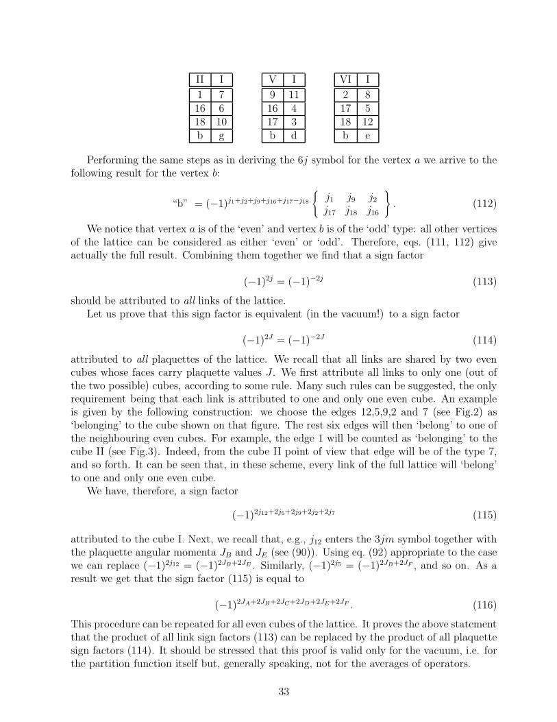
II I
1 716 618 10b g
V I
9 1116 417 3b d
VI I
2 817 518 12b e
Performing the same steps as in deriving the 6j symbol for the vertex a we arrive to thefollowing result for the vertex b:
“b” = (−1)j1+j2+j9+j16+j17−j18
j1 j9 j2
j17 j18 j16
. (112)
We notice that vertex a is of the ‘even’ and vertex b is of the ‘odd’ type: all other verticesof the lattice can be considered as either ‘even’ or ‘odd’. Therefore, eqs. (111, 112) giveactually the full result. Combining them together we find that a sign factor
(−1)2j = (−1)−2j (113)
should be attributed to all links of the lattice.Let us prove that this sign factor is equivalent (in the vacuum!) to a sign factor
(−1)2J = (−1)−2J (114)
attributed to all plaquettes of the lattice. We recall that all links are shared by two evencubes whose faces carry plaquette values J . We first attribute all links to only one (out ofthe two possible) cubes, according to some rule. Many such rules can be suggested, the onlyrequirement being that each link is attributed to one and only one even cube. An exampleis given by the following construction: we choose the edges 12,5,9,2 and 7 (see Fig.2) as‘belonging’ to the cube shown on that figure. The rest six edges will then ‘belong’ to one ofthe neighbouring even cubes. For example, the edge 1 will be counted as ‘belonging’ to thecube II (see Fig.3). Indeed, from the cube II point of view that edge will be of the type 7,and so forth. It can be seen that, in these scheme, every link of the full lattice will ‘belong’to one and only one even cube.
We have, therefore, a sign factor
(−1)2j12+2j5+2j9+2j2+2j7 (115)
attributed to the cube I. Next, we recall that, e.g., j12 enters the 3jm symbol together withthe plaquette angular momenta JB and JE (see (90)). Using eq. (92) appropriate to the casewe can replace (−1)2j12 = (−1)2JB+2JE . Similarly, (−1)2j5 = (−1)2JB+2JF , and so on. As aresult we get that the sign factor (115) is equal to
(−1)2JA+2JB+2JC+2JD+2JE+2JF . (116)
This procedure can be repeated for all even cubes of the lattice. It proves the above statementthat the product of all link sign factors (113) can be replaced by the product of all plaquettesign factors (114). It should be stressed that this proof is valid only for the vacuum, i.e. forthe partition function itself but, generally speaking, not for the averages of operators.
33
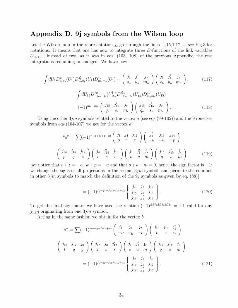
Appendix D. 9j symbols from the Wilson loop
Let the Wilson loop in the representation js go through the links ...,15,1,17,..., see Fig.3 fornotations. It means that one has now to integrate three D-functions of the link variablesU15,1,..., instead of two, as it was in eqs. (103, 108) of the previous Appendix, the restintegrations remaining unchanged. We have now
∫
dU1Dj1oaob
(U1)Dj′1
uaub(U1)D
js
mamb(U1) =
(
j1 j′1 js
oa ua ma
)(
j1 j′1 js
ob ub mb
)
, (117)
∫
dU15Dj15−qa,−qǫ
(U †15)D
j′15
−sa,−sǫ(U †
15)Djs
mbmǫ(U15)
= (−1)mǫ−ma
(
j15 j′15 js
qǫ sǫ mǫ
)(
j15 j′15 js
qa sa ma
)
. (118)
Using the other 3jm symbols related to the vertex a (see eqs.(99-102)) and the Kroneckersymbols from eqs.(104-107) we get for the vertex a:
“a” =∑
(−1)r+z+w+p−m
(
j1 j4 j12
o r z
)(
j′1 j13 j14
−u −w −p
)
(
j14 j15 j12
p q z
)(
j4 j′15 j13
r s w
)(
j1 j′1 js
o u m
)(
j15 j′15 js
q s m
)
(119)
[we notice that r + z = −o, w + p = −u and that o+u +m = 0, hence the sign factor is +1;we change the signs of all projections in the second 3jm symbol, and permute the columnsin other 3jm symbols to match the definition of the 9j symbols as given by eq. (88)]
= (−1)j′1−j4+j14+j15+js
j4 j1 j12
j′15 js j15
j13 j′1 j14
. (120)
To get the final sign factor we have used the relation (−1)±2j1±2j2±2j3 = +1 valid for anyj1,2,3 originating from one 3jm symbol.
Acting in the same fashion we obtain for the vertex b:
“b” =∑
(−1)−v−y−t−x+m
(
j1 j9 j2
−o −y −v
)(
j16 j18 j′1t x u
)
(
j16 j17 j9
t q y
)(
j18 j2 j′17x v s
)(
j1 j′1 so u m
)(
j17 j′17 js
q s m
)
= (−1)j′1−j2+j16+j17+js
j2 j1 j9
j′17 js j17
j18 j′1 j16
. (121)
34
References
[1] D.A.Varshalovich, A.N.Moskalev and V.K.Khersonskii, Quantum Theory of Angular
Momentum, World Scientific (1988)
[2] J.-M.Drouffe and J.-B.Zuber, Phys. Rep. 102 (1983) 1
[3] R.Anishety, S.Cheluvaraja and H.S.Sharatchandra, Phys. Lett. B314 (1993) 387
[4] I.G.Halliday and P.Suranyi, Phys. Lett. B350 (1995) 189
[5] M.B.Halpern, Phys. Rev. D16 (1977) 1798
[6] G.Ponzano and T.Regge, in: Spectroscopic and Group Theoretical Methods in Physics,ed. F.Bloch, North Holland, Amsterdam (1968)
[7] K.Schulten and R.G.Gordon, J. Math. Phys. 16 (1975) 1971
[8] T.Regge, Nuovo Cimento 19 (1961) 558
[9] E.Witten, Nucl. Phys. B311 (1988/89) 46
[10] F.A.Lunev, Phys. Lett. B295 (1992) 99
[11] P.E.Haagensen and K.Johnson, Nucl. Phys. B439 (1995) 597, hep-th/9408164;P.E.Haagensen, K.Johnson and C.S.Lam, Nucl. Phys. B477 (1996) 273, hep-th/9511226;R.Schiappa, Nucl. Phys. B517 (1998) 462, hep-th/9704206
[12] F.A.Lunev, J. Math. Phys. 37 (1996) 5351, hep-th/9503133
35