Cosmological observations in a modified theory of gravity (MOG

arX

iv:1

104.

2957

v2 [

astr

o-ph

.CO

] 4

Jan

201

2

January 5, 2012 1:10 WSPC/INSTRUCTION FILE ms

Cosmological observations in a modified theory of gravity (MOG)

J. W. Moffat1,2 and V. T. Toth11Perimeter Institute for Theoretical Physics, Waterloo, Ontario N2L 2Y5, Canada

2Department of Physics, University of Waterloo, Waterloo, Ontario N2L 3G1, Canada

Our modified gravity theory (MOG) is a gravitational theory without exotic dark matter,based on an action principle. MOG has been used successfully to model astrophysicalphenomena such as galaxy rotation curves, galaxy cluster masses, and lensing. MOG mayalso be able to account for cosmological observations. We assume that the MOG pointsource solution can be used to describe extended distributions of matter via an appro-priately modified Poisson equation. We use this result to model perturbation growth inMOG and find that it agrees well with the observed matter power spectrum at present.As the resolution of the power spectrum improves with increasing survey size, however,significant differences emerge between the predictions of MOG and the standard ΛCDMmodel, as in the absence of exotic dark matter, oscillations of the power spectrum inMOG are not suppressed. We can also use MOG to model the acoustic power spectrumof the cosmic microwave background. A suitably adapted semi-analytical model offersa first indication that MOG may pass this test, and correctly model the peak of theacoustic spectrum.

Keywords: Cosmology:theory — Large-scale structure of Universe — Gravitation.

1. Introduction

The preferred model of cosmology today, the ΛCDM model, provides an excellent

fit to cosmological observations, but at a substantial cost: according to this model,

about 95% of the universe is either invisible or undetectable, or possibly both1. This

fact provides a strong incentive to seek alternative explanations that can account

for cosmological observations without resorting to dark matter or Einstein’s cosmo-

logical constant.

For gravitational theories designed to challenge the ΛCDM model, the bar is set

increasingly higher by recent discoveries. Not only do such theories have to explain

successfully the velocity dispersions, rotational curves, and gravitational lensing of

galaxies and galaxy clusters, the theories must also be in accord with cosmolog-

ical observations, notably the acoustic power spectrum of the cosmic microwave

background (CMB), the matter power spectrum of galaxies, and the recent obser-

vation of the luminosity-distance relationship of high-z supernovae, which is seen

as evidence for “dark energy”.

Modified Gravity (MOG2) has been used successfully to account for galaxy

cluster masses3, the rotation curves of galaxies4,5, velocity dispersions of satellite

galaxies6, and globular clusters7. It was also used to offer an explanation for the

Bullet Cluster8 without resorting to nonbaryonic dark matter.

MOGmay also be able to meet the challenge posed by cosmological observations.

1

http://arxiv.org/abs/1104.2957v2


2

We investigate two sets of observations in particular: the matter power spectrum

that describes the spatial distribution of galaxies in the Universe, and the acoustic

spectrum of the cosmic microwave background (CMB) radiation.

In the next section, we review the key features of MOG. This is followed by

sections presenting detailed calculations for the galaxy power spectrum and the

acoustic power spectrum of the CMB. A concluding section summarizes our results

and maps out future steps.

2. Modified Gravity Theory

Modified Gravity (MOG) is a fully relativistic theory of gravitation that is derived

from a relativistic action principle2 involving scalar, tensor, and vector fields. MOG

has evolved as a result of investigations of Nonsymmetric Gravity Theory (NGT9),

and most recently, it has taken the form of Scalar-Tensor-Vector Gravity (STVG2).

In the weak field approximation, STVG, NGT, and Metric-Skew-Tensor Gravity

(MSTG10) produce similar results.

2.1. Scalar-Tensor-Vector Gravity

Our modified gravity theory is based on postulating the existence of a massive vector

field, φµ. The choice of a massive vector field is motivated by our desire to introduce

a repulsive modification of the law of gravitation at short range. The vector field is

coupled universally to matter. The theory, therefore, has three constants: in addition

to the gravitational constant G, we must also consider the coupling constant ω that

determines the coupling strength between the φµ field and matter, and a further

constant µ that arises as a result of considering a vector field of non-zero mass, and

controls the coupling range. The theory promotes G, µ, and ω to scalar fields, hence

they are allowed to run, resulting in the following action2,11.

S = SG + Sφ + SS + SM , (1)

where

SG = − 1

16π

∫

1

G(R+ 2Λ)

√−g d4x, (2)

Sφ = −∫

ω

[

1

4BµνBµν − 1

2µ2φµφ

µ + Vφ(φ)

]√−g d4x, (3)

SS =

∫

1

G

[

1

2gµν

(∇µG∇νG

G2+

∇µµ∇νµ

µ2−∇µω∇νω

)

− VG(G)

G2− Vµ(µ)

µ2− Vω(ω)

]√−g d4x. (4)

Here, SM is the “matter” action, while Bµν = ∂µφν − ∂νφµ, and Vφ(φ), VG(G),

Vω(ω), and Vµ(µ) denote the self-interaction potentials associated with the vector

field and the three scalar fields. The symbol ∇µ is used to denote covariant differen-

tiation with respect to the metric gµν , while the symbols R, Λ, and g represent the


3

Ricci-scalar, the cosmological constant, and the determinant of the metric tensor,

respectively. We define the Ricci tensor as

Rµν = ∂αΓαµν − ∂νΓ

αµα + Γα

µνΓβαβ − Γα

µβΓβαν . (5)

Our units are such that the speed of light, c = 1; we use the metric signature

(+,−,−,−).

The apparent “wrong” sign of the ∇µω∇µω term in the Lagrangian is of po-

tential concern; however, we found that in all the solutions (including numerical

solutions) considered to date, ω remains constant. Keeping ω as a dynamical scalar

field (with the “wrong” sign in the Lagrangian) allowed us to develop a parameter-

free solution11, but we anticipate that the ω field may disappear from the theory

as it is being further developed.

A direct numerical solution of the theory’s field equations in the spatially homo-

geneous, isotropic case (FLRW cosmology) yields an expanding universe. Choosing

a constant VG as one of the initial parameters of the solution, the age of the universe

can be adjusted to fit observation. As an alternative, we also considered changing

the overall sign of the kinetic terms in SS ; this solution, which violates several en-

ergy conditions, but keeps the energy density ρ positive, is a “bouncing” cosmology

(indeed, a classical bouncing cosmology requires that some or all of the energy con-

ditions be violated). In this cosmology, the age of the universe since the bounce and

the density of the universe at the time of the bounce can be tuned by choosing an

appropriate constant VG. Either way, a solution in which the age of the universe

is in agreement with observation can be obtained. These solutions are a subject of

further study, which will be reported elsewhere.

2.2. Point particles in a spherically symmetric field

For a point particle moving in the spherically symmetric field of a gravitating source,

a particularly simple solution for the acceleration is obtained12:

r = −GNM

r2[

1 + α− α(1 + µr)e−µr]

, (6)

where M is the source mass, while α determines the strength of the “fifth force”

interaction, and µ controls its range. In prior work, α and µ were considered free

parameters that were fitted to data. Our recent work11 allows us to determine α

and µ as functions of the source mass M :

α =M

(√M + E)2

(

G∞

GN− 1

)

, (7)

and

µ =D√M

. (8)

This solution can be seen to satisfy the field equations in the spherically symmet-

ric case either numerically or by deriving an approximate solution analytically11.


4

The numerical values for D and E are determined by matching the result against

galaxy rotation curves11:

D ≃ 6250 M1/2⊙ kpc−1, (9)

E ≃ 25000 M1/2⊙ . (10)

The value of G∞ ≃ 20GN is set to ensure that at the horizon distance, the effective

strength of gravity is about 6 times GN , eliminating the need for cold dark matter

in cosmological calculations, as described in the previous section.

2.3. The MOG Poisson Equation

The acceleration law (6) is associated with the potential,

Φ = −G∞M

r

[

1− α

1 + αe−µr

]

= ΦN +ΦY , (11)

where

ΦN = −G∞M

r(12)

is the Newtonian gravitational potential with G∞ = (1+α)GN as the gravitational

constant, and

ΦY =α

1 + αG∞M

e−µr

r(13)

is the Yukawa-potential. These potentials are associated with the corresponding

Poisson and inhomogeneous Helmholtz equations, which are given by Ref. 8:

∇2ΦN (r) = 4πG∞ρ(r), (14)

(∇2 − µ2)ΦY (r) = −4πα

1 + αG∞ρ(r). (15)

Full solutions to these potentials are given by

ΦN (r) = −G∞

∫

ρ(r)

|r− r| d3r, (16)

ΦY (r) =α

1 + αG∞

∫

e−µ|r−r|ρ(r)

|r− r| d3r. (17)

These solutions can be verified against Eqs. (12) and (13) by applying the delta

function point source density ρ(r) = Mδ3(r).

Strictly speaking, (17) is a valid solution only when α is approximately constant.

For inhomogeneous matter distributions, α is expected to vary as a function of

matter density, and as such, this naive application of the spherically symmetric,

static vacuum solution to model extended distributions of matter breaks down.

However, for small perturbations of a homogeneous background, we expect (17)

to remain valid; this expectation can be verified once generalized (approximate)

solutions of the theory in the presence of matter become available.


5

Combining Eq. (11) with Eqs. (14) and (15) yields

∇2Φ = 4πGNρ(r) + µ2ΦY (r) (18)

= 4πGNρ(r) + αµ2GN

∫

e−µ|r−r|ρ(r)

|r− r| d3r,

containing, in addition to the usual Newtonian term, a nonlocal source term on the

right-hand side.

3. MOG and the matter power spectrum

The distribution of mass in the universe is not uniform. Due to gravitational self-

attraction, matter tends to “clump” into ever denser concentrations, leaving large

voids in between. In the early universe, this process is counteracted by pressure.

The process is further complicated by the fact that in the early universe, the energy

density of radiation was comparable to that of matter.

3.1. Density fluctuations in Newtonian gravity

To first order, this process can be investigated using perturbation theory. Taking

an arbitrary initial distribution, one can proceed to introduce small perturbations

in the density, velocity, and acceleration fields. These lead to a second-order dif-

ferential equation for the density perturbation that can be solved analytically or

numerically. This yields the transfer function, which determines how an initial den-

sity distribution evolves as a function of time in the presence of small perturbations.

3.1.1. Newtonian theory of small fluctuations

In order to see how this theory can be developed for MOG, we must first review how

the density perturbation equation is derived in the Newtonian case. Our treatment

follows closely the approach presented by Ref. 13. We begin with three equations:

the continuity equation, the Euler equation, and the Poisson equation.

∂ρ

∂t+∇ · (ρv) = 0, (19a)

∂v

∂t+ (v · ∇)v = −1

ρ∇p+ g, (19b)

∇ · g = −4πGρ. (19c)

First, we perturb ρ, p, v and g. Spelled out in full, we get:

∂(ρ+ δρ)

∂t+∇ · [(ρ+ δρ)(v + δv)] = 0, (20a)

∂(v + δv)

∂t+ [(v + δv) · ∇](v + δv) = − 1

ρ+ δρ∇(p+ δp) + g+ δg, (20b)

∇ · (g + δg) = −4πG(ρ+ δρ). (20c)


6

Subtracting the original set of equations from the new set, using 1/(ρ + δρ) =

(ρ− δρ)/[ρ2 − (δρ)2] = 1/ρ− δρ/ρ2, and eliminating second-order terms, we obtain

∂δρ

∂t+∇ · (δρv + ρδv) = 0, (21a)

∂δv

∂t+ (v · ∇)δv + (δv · ∇)v =

δρ

ρ2∇p− 1

ρ∇δp+ δg, (21b)

∇ · δg = −4πGδρ. (21c)

A further substitution can be made by observing that δp = (δp/δρ)δρ = c2sδρ

where c2s = (∂p/∂ρ)adiabatic is the speed of sound. We can also eliminate terms

by observing that the original (unperturbed) state is spatially homogeneous, hence

∇ρ = ∇p = 0:

∂δρ

∂t+ v · ∇δρ+ δρ∇ · v + ρ∇ · δv = 0, (22a)

∂δv

∂t+ (v · ∇)δv + (δv · ∇)v = −c2s

ρ∇δρ+ δg, (22b)

∇ · δg = −4πGδρ. (22c)

Now we note that v = Hx, hence

∇ · v = H∇ · x = 3H,

(δv · ∇)v = (δv · ∇)(Hx) = H(δv · ∇)x = Hδv.

Therefore,

∂δρ

∂t+ v · ∇δρ+ 3Hδρ+ ρ∇ · δv = 0, (23a)

∂δv

∂t+ (v · ∇)δv +Hδv = −c2s

ρ∇δρ+ δg, (23b)

∇ · δg = −4πGδρ. (23c)

The next step is a change of spatial coordinates to coordinates comoving with the

Hubble flow:

x = a(t)q.

This means(

∂

∂t

)

q

=

(

∂

∂t

)

x

+ v∇x,

and

∇q = a∇x.


7

After this change of coordinates, our system of equations becomes

∂δρ

∂t+ 3Hδρ+

1

aρ∇ · δv = 0, (27a)

∂δv

∂t+Hδv = − c2s

aρ∇δρ+ δg, (27b)

∇ · δg = −4πaGδρ. (27c)

Now is the time to introduce the fractional amplitude δ = δρ/ρ. Dividing (27a)

with ρ, we get

δ +ρ

ρδ + 3Hδ +

1

a∇ · δv = 0. (28)

However, since ρ = ρ0a30/a

3, and hence ρ/ρ = −3a/a, the second and third terms

cancel, to give

−aδ = ∇δv. (29)

Taking the gradient of (27b) and using (27c) to express ∇ · δg, we get

∂

∂t(−aδ) +H(−aδ) = −c2s

a∇2δ − 4πGaρδ. (30)

Spelling out the derivatives, and dividing both sides with a, we obtain

δ + 2Hδ − c2sa2

∇2δ − 4πGρδ = 0. (31)

For every Fourier mode δ = δk(t)eik·q (such that ∇2δ = −k2δ), this gives

δk + 2Hδk +

(

c2sk2

a2− 4πGρ

)

δk = 0. (32)

The quantity k/a is called the co-moving wave number.

If k is large, solutions to (32) are dominated by an oscillatory term; for small k,

a growth term predominates.

A solution to (32) tells us how a power spectrum evolves over time, as a function

of the wave number; it does not specify the initial power spectrum. For this reason,

solutions to (32) are typically written in the form of a transfer function

T (k) =δk(z = 0)δ0(z = ∞)

δk(z = ∞)δ0(z = 0). (33)

If the initial power spectrum and the transfer function are known, the power

spectrum at a later time can be calculated (without accounting for small effects) as

P (k) = T 2(k)P0(k). (34)

P (k) is a dimensioned quantity. It is possible to form the dimensionless power

spectrum

∆2(k) = Ak3T 2(k)P0(k), (35)


8

where A is a normalization constant determined by observation. This form often

appears in the literature. In the present work, however, we are using P (k) instead

of ∆(k).

The initial power spectrum is believed to be a scale invariant power spectrum:

P0(k) ∝ kn, (36)

where n ≃ 1. A recent estimate1 on n is n = 0.963+0.014−0.015.

3.1.2. Analytical approximation

Eq. (32) is not difficult to solve in principle. The solution can be written as the

sum of oscillatory and growing terms. The usual physical interpretation is that

when pressure is sufficient to counteract gravitational attraction, this mechanism

prevents the growth of density fluctuations, and their energy is dissipated instead

in the form of sound waves. When the pressure is low, however, the growth term

dominates and fluctuations grow. Put into the context of an expanding universe,

one can conclude that in the early stages, when the universe was hot and dense, the

oscillatory term had to dominate. Later, the growth term took over, the perturbation

spectrum “froze”, affected only by uniform growth afterwards.

In practice, several issues complicate the problem. First, the early universe can-

not be modeled by matter alone; it contained a mix of matter and radiation (and,

possibly, neutrinos and cold dark matter.) To correctly describe this case even using

the linear perturbation theory outlined in the previous sections, one needs to re-

sort to a system of coupled differential equations describing the different mediums.

Second, if the perturbations are sufficiently strong, linear theory may no longer be

valid. Third, other nonlinear effects, including Silk-damping14, cannot be excluded

as their contribution is significant (indeed, Silk damping at higher wave numbers is

one of the reasons why a baryon-only cosmological model based on Einstein’s theory

of gravity without dark matter fails to account for the matter power spectrum.)

The authors of Ref. 15 addressed all these issues when they developed a semi-

analytical solution to the baryon transfer function. This solution reportedly yields

good results in the full range of 0 ≤ Ωb ≤ 1. Furthermore, unlike other approx-

imations and numerical software codes, this approach keeps the essential physics

transparent, allowing us to adapt the formulation to the MOG case.

In Ref. 15 the transfer function is written as the sum of a baryonic term Tb and

a cold dark matter term Tc:

T (k) =Ωb

ΩmTb(k) +

Ωc

ΩmTc(k), (37)

where Ωc represents the cold dark matter content of the universe relative to the crit-

ical density. As we are investigating a cosmology with no cold dark matter, we ignore

Tc. The baryonic part of the transfer function departs from the cold dark matter

case on scales comparable to, or smaller than, the sound horizon. Consequently, the


9

baryonic transfer function is written as

Tb(k) =

[

T0(k, 1, 1)

1 + (ks/5.2)2+

αbe−(k/kSilk)

1.4

1 + (βb/ks)3

]

sin ks

ks, (38)

with

T0(k, αc, βc) =ln (e+ 1.8βcq)

ln (e+ 1.8βcq) + Cq2, (39)

where

C =14.2

αc+

386

1 + 69.9q1.08, (40)

and

q = kΘ22.7

(

Ωmh2)−1

. (41)

The sound horizon is calculated as

s =2

3keq

√

G

Reqln

√1 +Rd +

√

Rd +Req

1 +√

Req

. (42)

The scale at the equalization epoch is calculated as

keq = 7.46× 10−2Ωmh2Θ−22.7. (43)

The transition from a radiation-dominated to a matter-dominated era happens at

the redshift

zeq = 25000Ωmh2Θ−42.7, (44)

while the drag era is defined as

zd = 1291(Ωmh2)0.251

1 + 0.659(Ωmh2)0.828[1 + b1(Ωmh2)b2 ], (45)

where

b1 = 0.313(Ωmh2)−0.419[1 + 0.607(Ωmh2)0.674], (46)

and

b2 = 0.238(Ωmh2)0.223. (47)

The baryon-to-photon density ratio at a given redshift is calculated as

R = 31.5Ωmh2Θ−42.7

1000

z. (48)

The Silk damping scale is obtained using

kSilk = 1.6(Ωbh2)0.52(Ωmh2)0.73[1 + (10.4Ωmh2)−0.95]. (49)

The coefficients in the second term of the baryonic transfer function are written as

αb = 2.07keqs(1 +Rd)−3/4F

(

1 + zeq1 + zd

)

, (50)


10

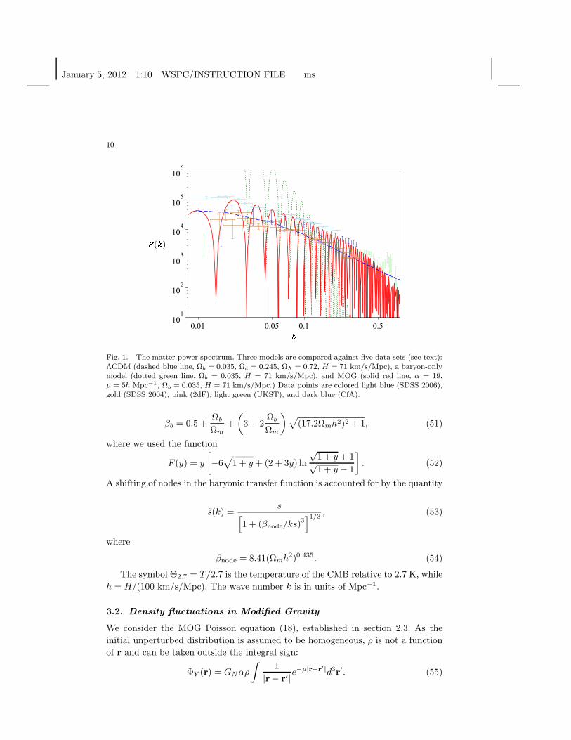
Fig. 1. The matter power spectrum. Three models are compared against five data sets (see text):ΛCDM (dashed blue line, Ωb = 0.035, Ωc = 0.245, ΩΛ = 0.72, H = 71 km/s/Mpc), a baryon-onlymodel (dotted green line, Ωb = 0.035, H = 71 km/s/Mpc), and MOG (solid red line, α = 19,µ = 5h Mpc−1, Ωb = 0.035, H = 71 km/s/Mpc.) Data points are colored light blue (SDSS 2006),gold (SDSS 2004), pink (2dF), light green (UKST), and dark blue (CfA).

βb = 0.5 +Ωb

Ωm+

(

3− 2Ωb

Ωm

)

√

(17.2Ωmh2)2 + 1, (51)

where we used the function

F (y) = y

[

−6√

1 + y + (2 + 3y) ln

√1 + y + 1√1 + y − 1

]

. (52)

A shifting of nodes in the baryonic transfer function is accounted for by the quantity

s(k) =s

[

1 + (βnode/ks)3]1/3

, (53)

where

βnode = 8.41(Ωmh2)0.435. (54)

The symbol Θ2.7 = T/2.7 is the temperature of the CMB relative to 2.7 K, while

h = H/(100 km/s/Mpc). The wave number k is in units of Mpc−1.

3.2. Density fluctuations in Modified Gravity

We consider the MOG Poisson equation (18), established in section 2.3. As the

initial unperturbed distribution is assumed to be homogeneous, ρ is not a function

of r and can be taken outside the integral sign:

ΦY (r) = GNαρ

∫

1

|r− r′|e−µ|r−r′|d3r′. (55)


11

Varying ρ, we get

∇ · δg(r) = −4πGNδρ(r)

−µ2GNαδρ

∫

1

|r− r′|e−µ|r−r′|d3r′. (56)

Accordingly, (31) now reads

δ + 2Hδ − c2sa2

∇2δ − 4πGNρδ − µ2GNαρδ

∫

e−µ|r−r′|

|r− r′| d3r′ = 0. (57)

The integral can be readily calculated. Assuming that |r − r′| runs from 0 to the

comoving wavelength a/k, we get

∫

e−µ|r−r′|

|r− r′| d3r′ = 2

π/2∫

0

2π∫

0

a/k∫

0

e−µr

rr2 sin θ dr dφ dθ

=4π

[

1− (1 + µa/k)e−µa/k]

µ2. (58)

Substituting into (57), we get

δ + 2Hδ − c2sa2

∇2δ − 4πGNρδ

− 4πGNα[

1−(

1 +µa

k

)

e−µa/k]

ρδ = 0, (59)

or

δ + 2Hδ − c2sa2

∇2δ (60)

−4πGN

1 + α[

1−(

1 +µa

k

)

e−µa/k]

ρδ = 0.

This demonstrates how the effective gravitational constant

Geff = GN

1 + α[

1−(

1 +µa

k

)

e−µa/k]

(61)

depends on the wave number.

Using Geff , we can express the perturbation equation as

δk + 2Hδk +

(

c2sk2

a2− 4πGeffρ

)

δk = 0. (62)

As the wave number k appears only in the source term(

c2sk2

a2− 4πGeffρ

)

,

it is easy to see that any solution of (32) is also a solution of (62), provided that k

is replaced by k′ in accordance with the following prescription:

k′2 = k2 + 4πa2(

Geff −GN

GN

)

λ−2J , (64)


12

where λJ =√

c2s/GNρ is the Jeans wavelength.

This shifting of the wave number applies to the growth term of the baryonic

transfer function (38). However, as the sound horizon scale is not affected by changes

in the effective gravitational constant, terms containing the product ks must remain

unchanged. Furthermore, the Silk damping scale must also change as a result of

changing gravity; this change is proportional to the 3/4th power of G, as demon-

strated bya Ref. 14, thus

k′Silk = kSilk

(

Geff

GN

)3/4

, (65)

(note also Eq. 49). Using these considerations, we obtain the modified baryonic

transfer function

T ′b(k) =

sin ks

ks

T0(k′, 1, 1)

1 + (ks/5.2)2+

αb exp(

−[k/k′Silk]1.4

)

1 + (βb/ks)3

. (66)

The effects of these changes can be summed up as follows. At low values of k,

the transfer function is suppressed. At high values of k, where the transfer function

is usually suppressed by Silk damping, the effect of this suppression is reduced. The

combined result is that the tilt of the transfer function changes, such that its peaks

are now approximately in agreement with data points, as seen in Figure 1.

Data points shown in this figure come from several sources. First and foremost,

the two data releases of the Sloan Digital Sky Survey (SDSS16,17) are presented.

Additionally, data from the 2dF Galaxy Redshift Survey18, UKST19, and CfA13020

surveys are shown. Apart from normalization issues, the data from these surveys are

consistent in the range of 0.01 h Mpc−1 ≤ k ≤ 0.5 h Mpc−1. Some surveys provide

data points outside this range, but they are not in agreement with each other.

3.3. Discussion

As a result of the combined effects of dampened structure growth at low values of

k and reduced Silk damping at high values of k, the slope of the MOG transfer

function differs significantly from the slope of the baryonic transfer function, and

matches closely the observed values of the matter power spectrum. On the other

hand, the predictions of MOG and ΛCDM cosmology differ in fundamental ways.

First, MOG predicts oscillations in the power spectrum, which are not smoothed

out by dark matter. These oscillations may be detectable in future galaxy surveys

that utilize a large enough number of galaxies, and sufficiently narrow window

functions in order to be sensitive to such fluctuations. However, the finite size of

samples and the associated window functions used to produce presently available

power spectra mask any such oscillations. To illustrate this, we applied the same

window function to the MOG prediction, which resulted in a smoothed curve, seen in

acf. Eq. (4.210) in Ref. 14; note that Ωh2∝ G.


13

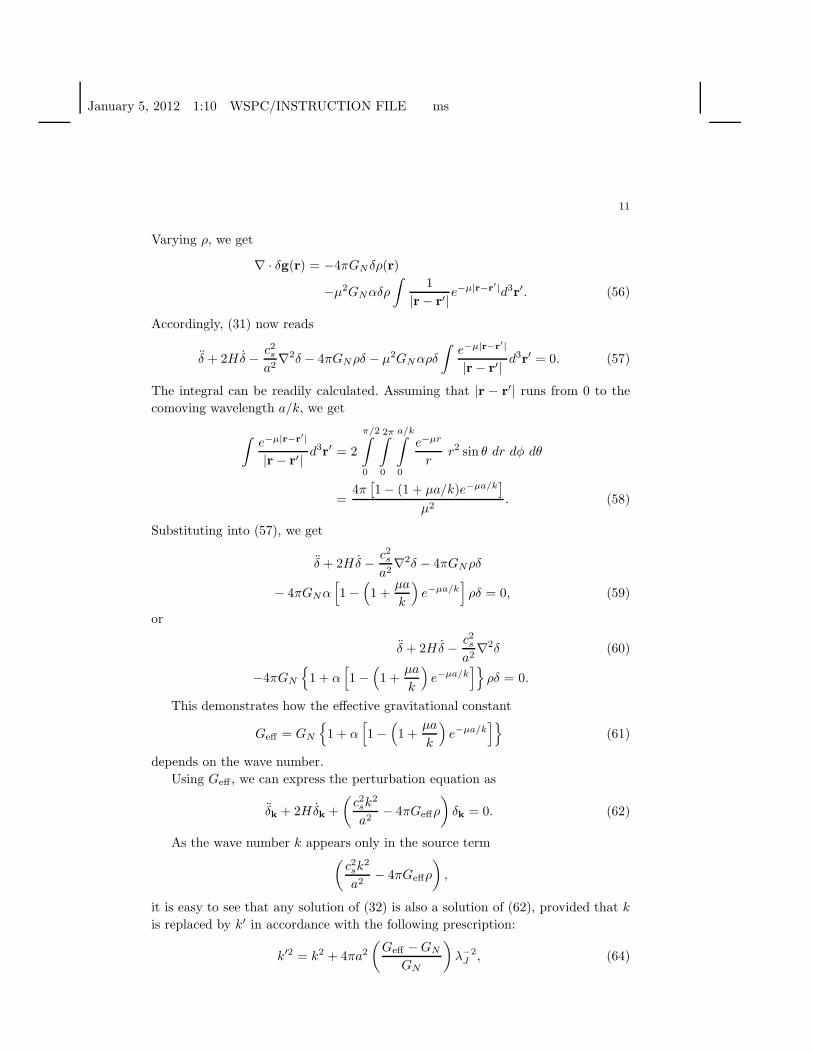
Fig. 2. The effect of window functions on the power spectrum is demonstrated by applying theSDSS luminous red galaxy survey window functions to the MOG prediction. Baryonic oscillationsare greatly dampened in the resulting curve (solid red line). A normalized linear ΛCDM estimateis also shown (thin blue line) for comparison.

Figure 2. A χ2 comparison actually suggests that MOG offers a better fit (χ2MOG =

0.03, χ2ΛCDM = 0.09 per degrees of freedom), although we must be cautious: the

ΛCDM approximation we used is not necessarily the best approximation available,

and the MOG result is dependent on the validity of the analysis presented in this

section, which was developed without the benefit of an interior solution.

Second, MOG predicts a dampened power spectrum at both high and low values

of k relative to ΛCDM. Observations at sufficiently high values of k may not be

practical, as we are entering sub-galactic length scales. Low values of k are a different

matter: as accurate three-dimensional information becomes available on ever more

distant galaxies, power spectrum observations are likely to be extended in this

direction.

In the present work, we made no attempt to account for the possibility of a non-

zero neutrino mass, and its effects on the power spectrum. Given the uncertainties

in the semi-analytical approximations that we utilized, such an attempt would not

have been very fruitful. Future numerical work, however, must take into account

the possibility of a non-negligible contribution of neutrinos to the matter density.

4. MOG and the CMB

The cosmic microwave background (CMB) is highly isotropic, showing only small

temperature fluctuations as a function of sky direction. These fluctuations are not

uniformly random; they show a distinct dependence on angular size, as has been

demonstrated by the measurements of the Boomerang experiment21 and the Wilkin-

son Microwave Anisotropy Probe (WMAP1).

The angular power spectrum of the CMB can be calculated in a variety of ways.


14

The preferred method is to use numerical software, such as CMBFAST22. Unfortu-

nately, such software packages cannot easily be adapted for use with MOG. Instead,

at the present time we opt to use the excellent semi-analytical approximation de-

veloped by Ref. 23. While not as accurate as numerical software, it lends itself more

easily to nontrivial modifications, as the physics remains evident in the equations.

What justifies the use of this semi-analytical approach is the fact that the phe-

nomenology of MOG vs. dark matter can be understood easily. Collisionless cold

dark matter interacts with normal matter only through gravity. In the late universe,

the ratio of cold dark matter vs. baryonic matter varies significantly from region to

region; this is why the results of the previous section are nontrivial and significant.

However, in the early universe (recombination era), the universe was still largely

homogeneous, and cold dark matter effectively acted as a “gravity enhancer”: its

effects can be mimicked by simply increasing the effective gravitational constant.

This may seem surprising in view of studies that have placed stringent con-

straints on the variability of G. For example, after substituting G → λ2G in the

Friedmann equation, the authors of Ref. 24 have shown that λ is constrained to 10%

or better by WMAP data. At first sight, this seems inconsistent with our assertion

that MOG, with Geff > GN , can successfully mimic the effects of dark matter on

the CMB acoustic spectrum. Yet that this is the case can be seen if one writes down

the Friedmann equation after incorporating λ:

H2 ∼ 8π

3λ2Gρ.

The full form of the substitution rule, therefore, is Gρ → λ2Gρ. In MOG, we sub-

stitute G → Geff and ρ → ρb (no CDM component), but (Gρ)ΛCDM = (Geffρb)MOG,

hence λ ≡ 1.

This discussion leads to a simple substitution rule that is applicable when the

universe is approximately homogeneous. When a quantity containing G appears

in an equation describing a gravitational interaction, Geff must be used. However,

when a quantity like Ωb is used to describe a nongravitational effect, the Newtonian

value of GN must be retained.

Our choice to use Mukhanov’s semianalytical approximation is motivated by the

fact that these substitutions can be made in the formulae in a straightforward and

unambiguous manner.

4.1. Semi-analytical estimation of CMB anisotropies

In Ref. 23 we find a calculation of the correlation function C(l), where l is the

multipole number, of the acoustic power spectrum of the CMB using the solution

C(l)

[C(l)]low l=

100

9(O +N), (67)


15

where l ≫ 1,O denotes the oscillating part of the spectrum, while the non-oscillating

part is written as the sum of three parts:

N = N1 +N2 +N3. (68)

These, in turn, are expressed as

N1 = 0.063ξ2[P − 0.22(l/lf)

0.3 − 2.6]2

1 + 0.65(l/lf)1.4e−(l/lf )

2

, (69)

N2 =0.037

(1 + ξ)1/2[P − 0.22(l/ls)

0.3 + 1.7]2

1 + 0.65(l/ls)1.4e−(l/ls)

2

, (70)

N3 =0.033

(1 + ξ)3/2[P − 0.5(l/ls)

0.55 + 2.2]2

1 + 2(l/ls)2e−(l/ls)

2

. (71)

The oscillating part of the spectrum is written as

O = e−(l/ls)2

√

π

ρl

×[

A1 cos(

ρl +π

4

)

+A2 cos(

2ρl +π

4

)]

, (72)

where

A1 = 0.1ξ(P − 0.78)2 − 4.3

(1 + ξ)1/4e

1

2(l−2

s −l−2

f )l2 , (73)

and

A2 = 0.14(0.5 + 0.36P )2

(1 + ξ)1/2. (74)

The parameters that occur in these expressions are as follows. First, the baryon

density parameter:

ξ = 17(

Ωbh275

)

, (75)

where Ωb ≃ 0.035 is the baryon content of the universe at present relative to the

critical density, and h75 = H/(75 km/s/Mpc). The growth term of the transfer

function is represented by

P = lnΩ−0.09

m l

200√

Ωmh275

, (76)

where Ωm ≃ 0.3 is the total matter content (baryonic matter, neutrinos, and cold

dark matter). The free-streaming and Silk damping scales are determined, respec-

tively, by

lf = 1300[

1 + 7.8× 10−2(

Ωmh275

)−1]1/2

Ω0.09m , (77)

ls =0.7lf

√

1+0.56ξ1+ξ + 0.8

ξ(1+ξ)

(Ωmh2

75)1/2

[

1+(1+ 100

7.8 Ωmh2

75)−1/2

]

2

. (78)


16

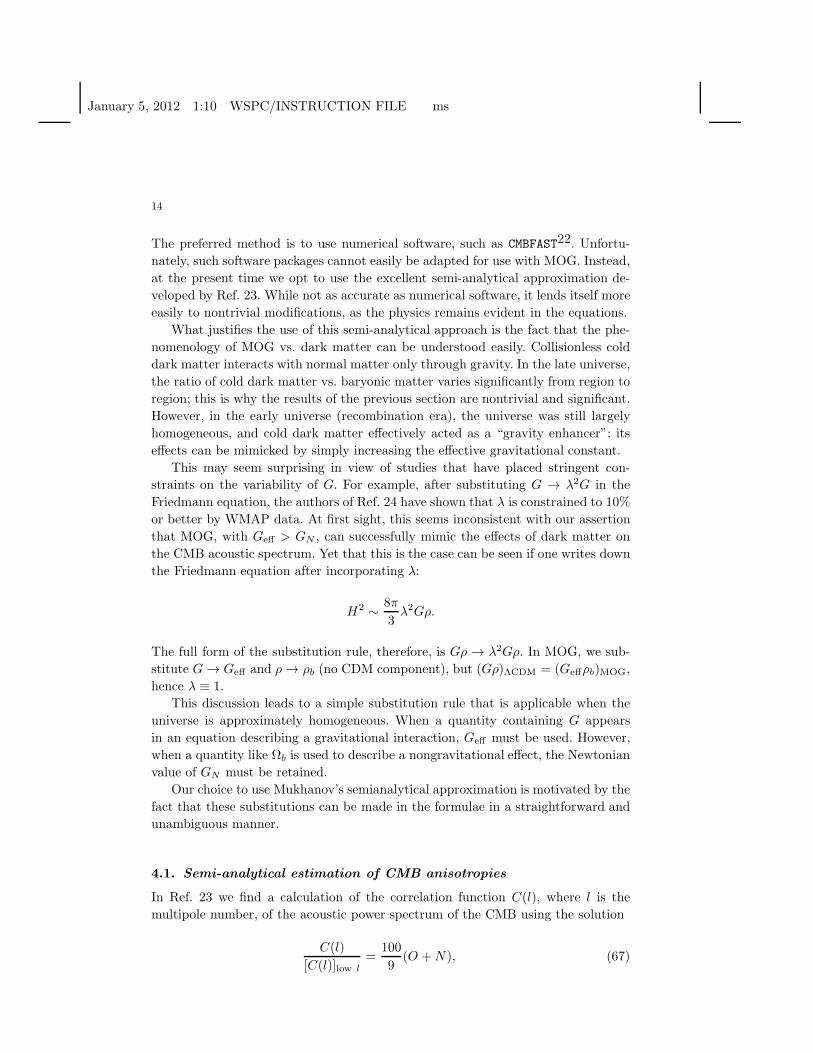
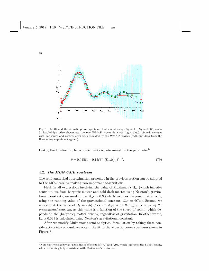
Fig. 3. MOG and the acoustic power spectrum. Calculated using ΩM = 0.3, Ωb = 0.035, H0 =71 km/s/Mpc. Also shown are the raw WMAP 3-year data set (light blue), binned averageswith horizontal and vertical error bars provided by the WMAP project (red), and data from theBoomerang experiment (green).

Lastly, the location of the acoustic peaks is determined by the parameterb

ρ = 0.015(1 + 0.13ξ)−1(Ωmh3.175 )

0.16. (79)

4.2. The MOG CMB spectrum

The semi-analytical approximation presented in the previous section can be adapted

to the MOG case by making two important observations.

First, in all expressions involving the value of Mukhanov’s Ωm (which includes

contributions from baryonic matter and cold dark matter using Newton’s gravita-

tional constant), we need to use ΩM ≃ 0.3 (which includes baryonic matter only,

using the running value of the gravitational constant, Geff ≃ 6GN ). Second, we

notice that the value of Ωb in (75) does not depend on the effective value of the

gravitational constant, as this value is a function of the speed of sound, which de-

pends on the (baryonic) matter density, regardless of gravitation. In other words,

Ωb ≃ 0.035 is calculated using Newton’s gravitational constant.

After we modify Mukhanov’s semi-analytical formulation by taking these con-

siderations into account, we obtain the fit to the acoustic power spectrum shown in

Figure 3.

bNote that we slightly adjusted the coefficients of (77) and (79), which improved the fit noticeably,while remaining fully consistent with Mukhanov’s derivation.


17

4.3. Discussion

As Figure 3 demonstrates, to the extent that Mukhanov’s formulation is applicable

to MOG, the theory achieves agreement with the observed acoustic power spectrum.

This result was obtained without fine-tuning or parameter fitting. The MOG con-

stant µ was assumed to be equal to the inverse of the radius of the visible universe.

Thereafter, the value of α is fixed if we wish to ensure ΩM ≃ 0.3. This was sufficient

to achieve consistency with the data.

5. Conclusions

In this paper, we demonstrated how MOG can account for key cosmological obser-

vations using a minimum number of free parameters. We applied the MOG point

source solution in a suitably modified form of the Poisson equation and re-derived

the equations of structure growth. We found that the result is in agreement with

presently available observational data.

Notably, we also found that as the available data sets grow in size, a significant,

and likely irreconcilable disagreement emerges between the predictions of MOG

and those of the ΛCDM concordance model. In ΛCDM, the presence of collisionless

exotic dark matter leads to a significant dampening of the baryonic oscillations in

the matter power spectrum: unit oscillations are suppressed, and appear only as a

slight modulation of the power spectrum at shorter wavelengths. In contrast, unit

oscillations are not suppressed in MOG. Presently, these oscillations are not seen

only because the resolution of the data is not high enough: when we apply the

appropriate bin sizes and window functions to a simulated data set, the resulting

curve is nearly smooth. As galaxy surveys grow in size, however, bin sizes will get

smaller and, if MOG is correct, the unit oscillations will emerge in the data.

We also investigated the acoustic power spectrum of the cosmic microwave back-

ground using MOG. Existing software codes, notably the program CMBFAST22 and

its derivatives, are ill suited for this investigation as it is difficult to disentangle

the use of quantities proportional to Gρ in gravitational vs. nongravitational con-

texts. Before embarking on what seems to be a formidable task, we turned to a

semi-analytical approximation23. While many of the approximations employed by

Ref. 23 are not physically motivated, but numerical fitting formulae, nonetheless

the role played by quantities proportional to Gρ can be clearly discerned, and the

formulae can be suitably adapted. While we recognize that this is not a conclusive

result, we find it nonetheless encouraging that the CMB acoustic power spectrum

was faithfully reproduced.

In conclusion, we have demonstrated that cosmological observations of the mat-

ter power spectrum and the CMB acoustic spectrum do not trivially rule out MOG

as a possible alternative to the standard ΛCDM model of cosmology.


18

Acknowledgments

The research was partially supported by National Research Council of Canada.

Research at the Perimeter Institute for Theoretical Physics is supported by the

Government of Canada through NSERC and by the Province of Ontario through

the Ministry of Research and Innovation (MRI).

References

1. E. Komatsu, J. Dunkley, M. R. Nolta, C. L. Bennett, B. Gold, G. Hinshaw, N. Jarosik,D. Larson, M. Limon, L. Page, D. N. Spergel, M. Halpern, R. S. Hill, A. Kogut, S. S.Meyer, G. S. Tucker, J. L. Weiland, E. Wollack, and E. L. Wright. Five-Year WilkinsonMicrowave Anisotropy Probe (WMAP) Observations: Cosmological Interpretation.ArXiv, 0803.0547, March 2008.

2. J. W. Moffat. Scalar-tensor-vector gravity theory. Journal of Cosmology and Astropar-

ticle Physics, 2006(03):004, 2006.3. J. R. Brownstein and J. W. Moffat. Galaxy cluster masses without non-baryonic dark

matter. Mon. Not. R. Astron. Soc., 367:527–540, April 2006.4. J. R. Brownstein and J. W. Moffat. Galaxy Rotation Curves without Nonbaryonic

Dark Matter. Astrophys. J., 636:721–741, January 2006.5. J. R. Brownstein. Modified Gravity and the Phantom of Dark Matter. ArXiv,

0908.0040 [astro-ph.GA], 2009.6. J. W. Moffat and V. T. Toth. Testing modified gravity with motion of satellites around

galaxies. ArXiv, 0708.1264 [astro-ph], August 2007.7. J. W. Moffat and V. T. Toth. Testing modified gravity with globular cluster velocity

dispersions. Astrophys. J., 680:1158, June 2008.8. J. R. Brownstein and J. W. Moffat. The Bullet Cluster 1E0657-558 evidence shows

modified gravity in the absence of dark matter. Mon. Not. R. Astron. Soc., 382 (1):29–47, November 2007.

9. J. W. Moffat. A new nonsymmetric gravitational theory. Physics Letters B, 355:447–452, February 1995.

10. J. W. Moffat. Gravitational theory, galaxy rotation curves and cosmology withoutdark matter. Journal of Cosmology and Astroparticle Physics, 2005(5):003, May 2005.

11. J. W. Moffat and V. T. Toth. Fundamental parameter-free solutions in Modified Grav-ity. Class. Quant. Grav., 26:085002, 2009.

12. J. W. Moffat and V. T. Toth. The bending of light and lensing in modified gravity.Mon. Not. R. Astron. Soc., 397:1885–1992, 2009.

13. S. Weinberg. Gravitation and Cosmology. John Wiley & Sons, 1972.14. T. Padmanabhan. Structure formation in the universe. Cambridge University Press,

1993.15. D. J. Eisenstein and W. Hu. Baryonic Features in the Matter Transfer Function.

Astrophys. J., 496:605–+, March 1998.16. M. Tegmark, M. R. Blanton, M. A. Strauss, F. Hoyle, D. Schlegel, R. Scoccimarro,

M. S. Vogeley, D. H. Weinberg, I. Zehavi, A. Berlind, T. Budavari, A. Connolly, D. J.Eisenstein, D. Finkbeiner, J. A. Frieman, J. E. Gunn, A. J. S. Hamilton, L. Hui,B. Jain, D. Johnston, S. Kent, H. Lin, R. Nakajima, R. C. Nichol, J. P. Ostriker,A. Pope, R. Scranton, U. Seljak, R. K. Sheth, A. Stebbins, A. S. Szalay, I. Szapudi,L. Verde, Y. Xu, J. Annis, N. A. Bahcall, J. Brinkmann, S. Burles, F. J. Castander,I. Csabai, J. Loveday, M. Doi, M. Fukugita, J. R. I. Gott, G. Hennessy, D. W. Hogg,Z. Ivezic, G. R. Knapp, D. Q. Lamb, B. C. Lee, R. H. Lupton, T. A. McKay, P. Kunszt,


19

J. A. Munn, L. O’Connell, J. Peoples, J. R. Pier, M. Richmond, C. Rockosi, D. P.Schneider, C. Stoughton, D. L. Tucker, D. E. Vanden Berk, B. Yanny, and D. G.York. The Three-Dimensional Power Spectrum of Galaxies from the Sloan DigitalSky Survey. Astrophys. J., 606:702–740, May 2004.

17. M. Tegmark, D. J. Eisenstein, M. A. Strauss, D. H. Weinberg, M. R. Blanton, J. A.Frieman, M. Fukugita, J. E. Gunn, A. J. S. Hamilton, G. R. Knapp, R. C. Nichol, J. P.Ostriker, N. Padmanabhan, W. J. Percival, D. J. Schlegel, D. P. Schneider, R. Scoc-cimarro, U. Seljak, H.-J. Seo, M. Swanson, A. S. Szalay, M. S. Vogeley, J. Yoo, I. Ze-havi, K. Abazajian, S. F. Anderson, J. Annis, N. A. Bahcall, B. Bassett, A. Berlind,J. Brinkmann, T. Budavari, F. Castander, A. Connolly, I. Csabai, M. Doi, D. P.Finkbeiner, B. Gillespie, K. Glazebrook, G. S. Hennessy, D. W. Hogg, Z. Ivezic,B. Jain, D. Johnston, S. Kent, D. Q. Lamb, B. C. Lee, H. Lin, J. Loveday, R. H.Lupton, J. A. Munn, K. Pan, C. Park, J. Peoples, J. R. Pier, A. Pope, M. Richmond,C. Rockosi, R. Scranton, R. K. Sheth, A. Stebbins, C. Stoughton, I. Szapudi, D. L.Tucker, D. E. V. Berk, B. Yanny, and D. G. York. Cosmological constraints from theSDSS luminous red galaxies. Phys. Rev. D, 74(12):123507–+, December 2006.

18. S. Cole, W. J. Percival, J. A. Peacock, P. Norberg, C. M. Baugh, C. S. Frenk, I. Baldry,J. Bland-Hawthorn, T. Bridges, R. Cannon, M. Colless, C. Collins, W. Couch, N. J. G.Cross, G. Dalton, V. R. Eke, R. De Propris, S. P. Driver, G. Efstathiou, R. S. Ellis,K. Glazebrook, C. Jackson, A. Jenkins, O. Lahav, I. Lewis, S. Lumsden, S. Maddox,D. Madgwick, B. A. Peterson, W. Sutherland, and K. Taylor. The 2dF Galaxy RedshiftSurvey: power-spectrum analysis of the final data set and cosmological implications.Mon. Not. R. Astron. Soc., 362:505–534, September 2005.

19. F. Hoyle, C. M. Baugh, T. Shanks, and A. Ratcliffe. The Durham/UKST GalaxyRedshift Survey - VI. Power spectrum analysis of clustering. Mon. Not. R. Astron.

Soc., 309:659–671, November 1999.20. C. Park, M. S. Vogeley, M. J. Geller, and J. P. Huchra. Power spectrum, correla-

tion function, and tests for luminosity bias in the CfA redshift survey. Astrophys. J.,431:569–585, August 1994.

21. W. C. Jones, P. A. R. Ade, J. J. Bock, J. R. Bond, J. Borrill, A. Boscaleri, P. Cabella,C. R. Contaldi, B. P. Crill, P. de Bernardis, G. De Gasperis, A. de Oliveira-Costa,G. De Troia, G. di Stefano, E. Hivon, A. H. Jaffe, T. S. Kisner, A. E. Lange, C. J.MacTavish, S. Masi, P. D. Mauskopf, A. Melchiorri, T. E. Montroy, P. Natoli, C. B.Netterfield, E. Pascale, F. Piacentini, D. Pogosyan, G. Polenta, S. Prunet, S. Ricciardi,G. Romeo, J. E. Ruhl, P. Santini, M. Tegmark, M. Veneziani, and N. Vittorio. AMeasurement of the Angular Power Spectrum of the CMB Temperature Anisotropyfrom the 2003 Flight of BOOMERANG. Astrophys. J., 647:823–832, August 2006.

22. U. Seljak and M. Zaldarriaga. A Line-of-Sight Integration Approach to Cosmic Mi-crowave Background Anisotropies. Astrophys. J., 469:437–+, October 1996.

23. Viatcheslav Mukhanov. Physical Foundations of Cosmology. Cambridge UniversityPress, 2005.

24. O. Zahn and M. Zaldarriaga. Probing the Friedmann equation during recombinationwith future cosmic microwave background experiments. Phys. Rev. D, 67(6):063002–+, March 2003.

Cosmological observations in a modified theory of gravity (MOG

Documents

Transcript of Cosmological observations in a modified theory of gravity (MOG