Downward continuation of Helmert’s gravityP. Vanıcek1,W. Sun1;�, P. Ong1, Z. Martinec2, M. Najafi1, P. Vajda1, B. ter Horst3

1Department of Geodesy and Geomatics Engineering, University of New Brunswick, Box 4400 Frederiction, N.B. Canada E3B 5A32Department of Geophysics, Charles University, Prague, Czech Republic3Faculty of Geodesy, Delft Technical University, Delft, The Netherlands�Present address: Department of Geodesy and Photogrammetry, Royal Institute of Technology, S-100 44 Stockholm, Sweden

Received 27 October 1995; Accepted 9 July 1996

Abstract. The aim of this contribution is to show thatmean Helmert’s gravity anomalies obtained at the earthsurface on a grid of a ‘reasonable’ step can betransferred to corresponding mean Helmert’s anomalieson the geoid. To demonstrate this, we take the 50 by 50

mean Helmert’s anomalies from a very rugged region,the south-western corner of Canada which contains thetwo main chains of the Canadian Rocky Mountains,and formulate the problem of downward continuationof Helmert’s anomalies for this region. This can be doneexactly because Helmert’s disturbing potential is har-monic everywhere outside the geoid, therefore evenwithin the topography. Then we solve the problemnumerically by transforming the Poisson integral to asystem of 53,856 linear algebraic equations. Since thematrix of this system is well conditioned, there is notheoretical obstacle to the solution. The correctness ofthe solution is then checked by back substitution and byevaluating the contribution of the downward continua-tion term to Helmert’s co-geoid. This contributioncomes out positive for all the points. We thus claimthat the determination of the downward continuation ofmean Helmert’s gravity anomalies on a grid of a‘reasonable’ step is a well posed problem with a uniquesolution and can be done routinely to any accuracydesired in the geoid computaion.

1. Introduction

In the standard Stokes formulation of the geodeticboundary value problem, the solution (the disturbingpotential T) is sought above the boundary, the geoid,while the observations (gravity values g) are available onthe surface of the earth (Heiskanen and Moritz, 1967).To obtain the boundary values, the observations thushave to be reduced from the earth surface onto thegeoid. This reduction is in geodetic literature called thedownward continuation.

The downward continuation may be applied toobserved gravity values g, gravity disturbances dg,disturbing potential T, or any combination of thesequantities. Once we know how to downward continue T,the downward continuation of the other quantities canbe also derived. The main problem is that the spacethrough which we want to reduce the desired quantitycontains (topographical) masses with an irregulardensity distribution. It is relatively easy to downwardcontinue a harmonic function, but it is very difficult todo so with a non-harmonic one since we would have totake into account the density of topographical masses.While T is harmonic outside the earth surface (dis-regarding the atmospheric density), it is certainly notharmonic within the topography.

The way this problem is usually treated is totransform it into a model space, where the disturbingpotential to be dealt with is harmonic between the earthsurface and the geoid. Two such models have been usedin geodesy: the free-air model and the Helmert model.The former is employed in the context of solving theMolodenskij problem (Moritz, 1980) and it consists of‘‘moving’’ topographical masses inside the geoid so asnot to change the external potential. The downwardcontinuation performed by means of this model thusconstitutes the downward continuation of the externalfield T inside the topography (Vanıcek and Martinec1994). The latter model uses Helmert’s ‘‘condensation’’of topography onto the geoid by means of one of thecondensation techniques, that may preserve either thetotal mass of the earth, or the location of the centre ofmass, or to be just an integral mean of topographicalcolumn density – see, e.g., (Wichiencharoen 1982).

The open question in both these approaches is theexistence of the harmonic downward continuation of themodel field. In the free-air model, the model fieldcoincides with the real field on the earth surface and assuch is very complicated, because it is affected by thedensity irregularities in the close proximity of the earthsurface, i.e., within the topography. It thus hasconstituents of all spatial frequencies with possibly largeamplitudes. Yet, the physics the gravitational attractionin a region of harmonicity requires that constituents ofdifferent wave numbers n be suitably attenuated (by anapproximate factor of ��R � H�=R�n� when going fromthe geoid to the earth surface of height H above theCorrespondence to: P. Vanıcek

Journal of Geodesy (1996) 71: 21–34

geoid. In other words, there probably does not exist adisturbing potential ‘‘corresponding to free-air anom-aly’’ in the sense of eqn. (2), harmonic between the geoidand the earth surface, which would have the value T atthe surface. This problem is usually overcome by somesmoothing of T such as the Residual Terrain Modelmethod (Forsberg 1984), called also ‘‘regularization’’, atthe earth surface, the physical interpretation of which isunclear.

In the Helmert model, T is transformed to theHelmert disturbing potential Th by the followingequation

Th� T ÿ V ; �1�

where V is the difference between the potential of thetopography and the potential of the Helmert condensa-tion layer (Vanıcek and Martinec 1994; Martinec andVanıcek, 1994). Helmert’s disturbing potential at theearth surface is thus made smoother than the actualdisturbing potential because the nearest ‘‘disturbingmasses’’ are now located on the geoid. To illustrate thispoint, we show in Figure 1 a profile of free-air anomaly,defined to a spherical approximation as (Heiskanen andMoritz, 1967)

Dgfat _�ÿ

@T@r

����tÿ

2R

Tt; �2�

at the earth surface t taken across a particularly ruggedpart of the Canadian Rocky Mountains and compare itwith the same profile depicting the Helmert anomalyVanıcek and Martinec 1994)

Dght _�ÿ

@Th

@r

����tÿ

2R

Tht ; �3�

given again to a spherical approximation. Even for the50 step the smoothing effect of the ‘‘Helmertization’’ isalready visible. The real difference would be seen at thehigh frequency part of the respective spectra, from wavenumber n � 6; 000 onwards. The investigation of thisdifference is, however, not pertinent here.

The problem with the Helmertization of thedisturbing potential is that the direct topographicaleffect V cannot be evaluated exactly; the densitydistribution within topography is not known veryaccurately and some density model has to be assumed.In the first approximation a constant topographicaldensity of 2.67 g/cm3 is normally used and this is thedensity model we have used in the experiment reportedin this paper.

We note that eqn. (3) can be written also as (cf. eqn.(1))

Dght _�Dgfa

t �

@V@r

����t�

2R

Vt; �4�

where the second term on the right hand side is the directtopographical effect on gravity at the earth surface andthe third term is called the secondary indirect to-pographical effect on gravity at the earth surface. Theyboth are functions of topographical height H andtopographical density q (Vanıcek and Martinec, 1994)and can be evaluated numerically once a density modelis assumed and a condensation technique adopted.

Fig. 1. Profile of free-air (– � – �) andHelmert (–)50 � 50 gravity anomalies forlatitude / � 50�:417

22

2. Application of Poisson’s theorem

Let us now discuss the problem of ‘‘downwardcontinuation’’ from the mathematical point of view.The standard mathematical apparatus used in studyingdownward as well as upward continuation is the Poissontheorem. The Poisson theorem states that from afunction f, known on a sphere of radius R and harmonicoutside this sphere, we can compute the functional valuef�r;X� anywhere outside the sphere, i.e., for r > R bythe following (Poisson) integral (Kellogg 1929; Mac-Millan 1930)

f�r;X� �1

4p

Z

X0

f�R;X0�K�r;w;R�dX0

; �5�

where K is the Poisson’s kernel

K�r;w;R� �X1

j�0

�2j � 1�Rr

� �j�1

Pj�cos w�

� Rr2ÿ R2

l3 ;

�6�

w is the angular distance between geocentric directions Xand X0 and l is the spatial distance between �r;X� and�R;X0

�. This theorem can be directly applied to Th, if wethink the approximation of the geoid by the sphere ofradius R is admissible; it guarantees an accuracy betterthan 1.3 * 10ÿ3 which seems reasonable here.

An expression similar to (5) can be derived also forthe radial derivative of a harmonic function f (Heiska-nen and Moritz 1967)

@f@r

����r;X�

R4pr

Z

X0

@f@r

����R;X0

K�r;w;R�dX0: �7�

Again, to a spherical approximation of the geoid, thisexpression can be directly applied to the radialderivative of Th. But the radial derivative of Th isnothing else but Helmert’s gravity disturbance (Heiska-nen and Moritz 1967) dgh and we can write for theunknown Helmert’s gravity anomaly on the geoid(subscript g)

Dghg � Dgh

t � dghg ÿ dgh

t ÿ2R�Th

g ÿ Tht �

� Dght ÿ Ddgh

ÿ DTh;

�8�

where Ddhg is the downward continuation of Helmert’s

gravity disturbance called Dgh in (Vanıcek andMartinec 1994) and DTh is the downward continuationof 2Th

=R:Denoting the difference Dgh

g ÿ Dght by DDgh and

calling it the downward continuation of Helmert gravityanomaly, we can write eqn. (8) as

DDgh� ÿDdgh

ÿ DTh: �9�

This equation shows that the only difference between thedownward continuation of gravity disturbance and thatof gravity anomaly is the term DTh. This term

DTh�X� �

2R

Thg �X�

ÿ

12pR

Z

X0

Thg �X

0�K�r;w;R�dX0

�10�

is of a much lower spatial frequency than the Ddgh term.For the degree n of the model equal to 180, themagnitude of Th drops by two orders compared to Dgh

:

It is also much smaller and can thus be adequatelyevaluated from a global model. This can be seen on theplot in Figure 2 showing the south-western corner ofCanada that includes several chains of the RockyMountains.

3. Setting up the recursive formula

Since the (Helmert) gravity anomaly at the earth surfaceis more readily obtained than the (Helmert) gravitydisturbance, we shall work with gravity anomalies ratherthan gravity disturbances.

From the Poisson integrals for Th and @Th=@r; and

eqn. (3) we can easily derive the following expression

Dght _�

R4pr

Z

X0

DghgK�r;w;R�dX0

� I�Dghg�;

�11�

good to the usual spherical approximation. The problemof downward continuation is then reduced to thesolution of the above integral equation of first kind:Dgh

t is known and Dghg is to be determined.

Up to the sperical approximation, the integralequation (11) is valid exactly since Th is harmonic abovethe geoid. Hence a unique solution Dgh

g to eqn. (11)exists if Th

g (on the geoid) is finite and Dght is exact. From

the physics of the problem it should be obvious thatindeed Th

g is finite but it may have large amplitudes forshort wavelength components. As the solution of ourintegral equation (of first kind) is inherently unstable,any errors in Dgh

t may get amplified by the solution.Generally, the shorter wavelength errors will getamplified more than the longer wavelength ones. Toaleviate this problem, we apply a stabilizing procedureconsisting of using mean anomalies rather than pointanomalies. (The application of Stokes’s formula can beregarded as another stabilization process, of course) Weshall return to this problem at the end of this section.First, we set up a simple recurrence process to solve theintegral equation iteratively.

Let us begin by denoting

Dght ÿ I�Dgh

g� � q; �12�

clearly, according to eqn. (11), this difference equals to 0.We can define

q�k�1�� Dgh

t ÿ I �Dghg�

�k�h i

; �13�

where the superscript in brackets denotes the iterationnumber, and start the iterative process with

23

�Dghg�

�0�� q�0� � Dgh

t : �14�

We note that this implies

q�1� � Dght ÿ I�Dgh

t �: �15�

The sought quantity �Dght � is given by

Dghg � Dgh

t �X1

j�1

q�j� �X1

j�0

q�j� �16�

and its iterative approximations are

�Dghg�

�k��

Xk

j�0

q�j�: �17�

The recursive formula for one point X then can bewritten as

q�k�1��X� � Dgh

t �X� ÿR

4pr

Z

X0

Xk

j�0

q�j�K�r;w;R�dX0

� Dght �X� ÿ I

Xk

j�0

q�j� !

:

�18�

This equation can be easily converted to an operationalrecursive formula for the individual differences whichreads

q�k�1��X� � q�k��X� ÿ I�q�k��

� q�k��X� ÿR

4pr

Z

X0

q�k�K�r;w;R�dX0:

�19�

When we want to solve for the Dghg�X� in a certain

area A, we start the process by taking the knownHelmert anomaly on the surface of the earth as thezeroth iteration (eqn. (14)) for all the points X in A anduse eqn. (19) to compute the successive iterations, again,for all the points in A, till even the largest differenceqk�1

�X� in A is in absolute value smaller than aprescribed limit. This limit can be set up to perhapssome 10lGal, which should ensure that the accuracy ofgeoid computed from so determined anomalies wouldnot be affected above the magic 1cm level (Vanıcek andMartinec 1994). Let us note here, that there exist better,i.e., faster converging schemes. A search for the bestsuited scheme was not considered necessary in this initialstage of our investigations. One such technique waspointed to us ‘‘after the fact’’ by Vermeer (1995,personal communication) and will be tested in sub-sequent investigations.

There are two problems with the process describedabove. The first one concerns the convergence of theiterative process – none of the discussion in this sectiongives us any hint as to the convergence of the process.This means that based on the discussion above, wecannot guarantee that the largest difference in A willever be smaller than the prescribed limit. The potentialnon-convergence of the iterative process is related to the

Fig 2. The downward continuation of 2T/R (lGal). Contour interval = 10 lGal

24

above mentioned lack of stability of the solution. Wewill have more to say about it in sections 5 and 6.

The second problem is related to the integralappearing in eqn. (19) – this integral is to be taken overthe whole earth and thus the differences q�k�1�

�X� haveto be computed over the whole earth. We shall discussthe second problem in the next section.

4. Selecting integration limits

Fortunately, the Poisson kernel

K�r;w;R� � K�R � H ;w;R� � KHR;w

� �

�20�

that dominates the behaviour of the sub-integralfunction in eqn. (19), vanishes rather quickly withgrowing angular distance w – see Figure 3. This meansthat the integration in eqn. (19) can be taken only over aspherical cap of a relatively small radius w0 (instead ofover the whole earth) and the error committed by doingso – the integration truncation error which we will becalling here simply the truncation error – remainsrelatively small. This behaviour is governed by theheight H of the point X: the higher the point, the slowerthe kernel vanishes.

We have tested different truncation radii w0 for theirtruncation errors and determined that a truncationradius of 1� gives a reasonably small error for our testarea in south-western Canada. Moreover, the truncationerror can be reduced by introducing a modification ofthe Poisson kernel. The technique invented by Molo-denskij, where the upper limit of the truncation error isminimized (Molodenskij et al. 1960; Sjoberg 1984; eqn.13), appears to be well suited to our purpose. We shallnow show, how this technique works in our context.

We begin by rewriting the integral in eqn. (19) asZ

X0

q�k�K�X;X0�dX0

�

Z

C0

q�k�K�X;X0�dX0

�

Z

X0ÿC0

q�k�K�X;X0�dX0

; �21�

where C0 denotes the spherical cap of radius w0. Clearly,the second term in eqn. (21) is the truncation error to beminimized and we shall denote it by DgT . Theminimization is carried out in the sense of minimizingthe upper bound of the absolute value of the truncationerror (Vanıcek and Sjoberg 1991 eqn. (15)) bysubtracting from the Poisson’s kernel an appropriatelyselected linear combination of spherical harmonicfunctions taken to a degree and order L. We haveselected this upper limit to equal to 20. To be able to usethe Molodenskij modification, we have to subtract firstthe low degree harmonics (� L) from the function to beconvolved with the modified Poisson kernel. The lowdegree harmonics DgL have to be determined separatelyfrom a global gravity model and added to the truncationerror DgT , which is also determined from a globalgravity model. The determination of the appropriatecoefficients of the modifying linear combination, some

Fig. 3. Poisson’s integration kernel for heights H � 1; 000 m andH � 1 m. Note that the plots close to the computation point are inlog. scale

25

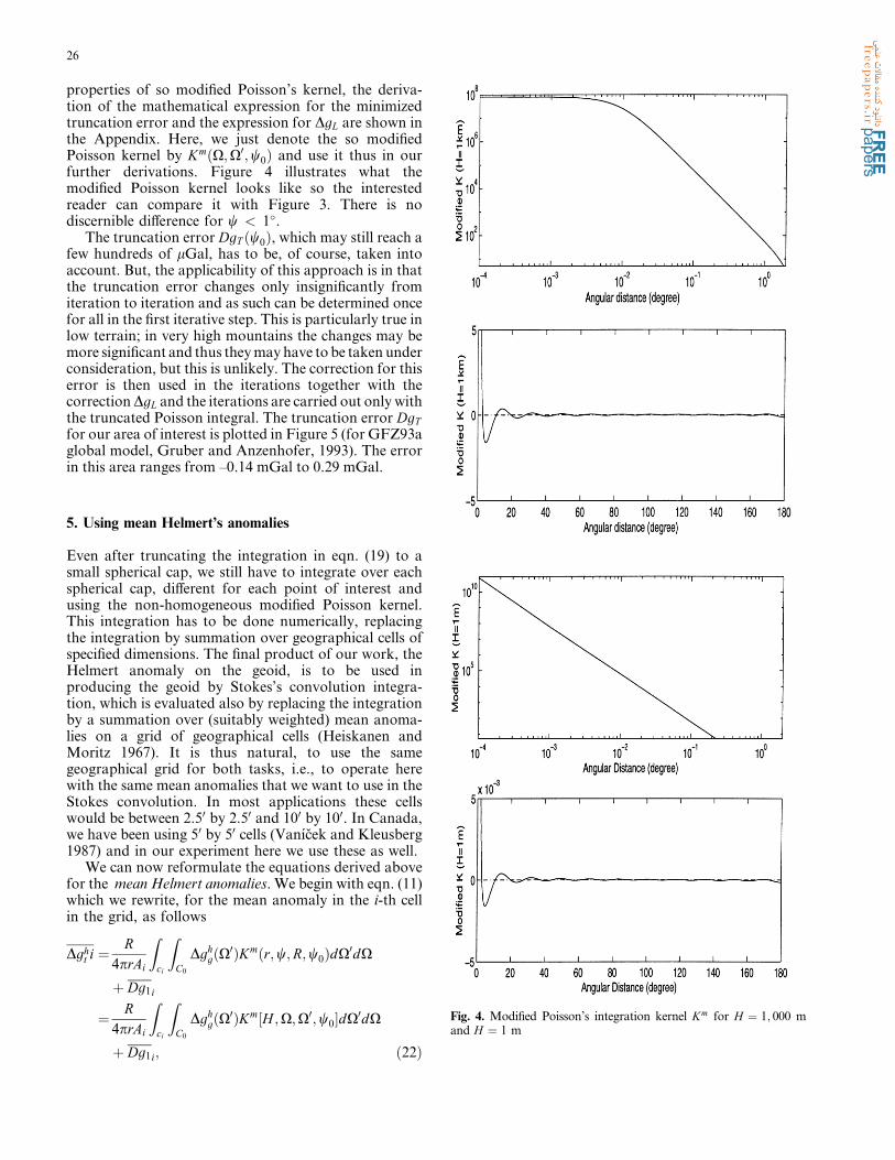
properties of so modified Poisson’s kernel, the deriva-tion of the mathematical expression for the minimizedtruncation error and the expression for DgL are shown inthe Appendix. Here, we just denote the so modifiedPoisson kernel by Km

�X;X0;w0� and use it thus in our

further derivations. Figure 4 illustrates what themodified Poisson kernel looks like so the interestedreader can compare it with Figure 3. There is nodiscernible difference for w < 1�.

The truncation error DgT �w0�, which may still reach afew hundreds of lGal, has to be, of course, taken intoaccount. But, the applicability of this approach is in thatthe truncation error changes only insignificantly fromiteration to iteration and as such can be determined oncefor all in the first iterative step. This is particularly true inlow terrain; in very high mountains the changes may bemore significant and thus they may have to be taken underconsideration, but this is unlikely. The correction for thiserror is then used in the iterations together with thecorrection DgL and the iterations are carried out only withthe truncated Poisson integral. The truncation error DgTfor our area of interest is plotted in Figure 5 (for GFZ93aglobal model, Gruber and Anzenhofer, 1993). The errorin this area ranges from –0.14 mGal to 0.29 mGal.

5. Using mean Helmert’s anomalies

Even after truncating the integration in eqn. (19) to asmall spherical cap, we still have to integrate over eachspherical cap, different for each point of interest andusing the non-homogeneous modified Poisson kernel.This integration has to be done numerically, replacingthe integration by summation over geographical cells ofspecified dimensions. The final product of our work, theHelmert anomaly on the geoid, is to be used inproducing the geoid by Stokes’s convolution integra-tion, which is evaluated also by replacing the integrationby a summation over (suitably weighted) mean anoma-lies on a grid of geographical cells (Heiskanen andMoritz 1967). It is thus natural, to use the samegeographical grid for both tasks, i.e., to operate herewith the same mean anomalies that we want to use in theStokes convolution. In most applications these cellswould be between 2.50 by 2.50 and 100 by 100. In Canada,we have been using 50 by 50 cells (Vanıcek and Kleusberg1987) and in our experiment here we use these as well.

We can now reformulate the equations derived abovefor the mean Helmert anomalies. We begin with eqn. (11)which we rewrite, for the mean anomaly in the i-th cellin the grid, as follows

Dght i �

R4prAi

Z

ci

Z

C0

Dghg�X

0�Km

�r;w;R;w0�dX0dX

� Dg1i

�

R4prAi

Z

ci

Z

C0

Dghg�X

0�Km

�H ;X;X0;w0�dX0dX

� Dg1i; �22�

Fig. 4. Modified Poisson’s integration kernel Km for H � 1; 000 mand H � 1 m

26

where ci denotes the i-th cell with area Ai and C0 denotesagain the spherical cap for the truncated integration.Note that since we use the modified Poisson kernelKm

�H ;w;w0�, the low frequency contribution is takenaway automatically from the first term of eqn. (22).Then the second term Dg1 in eqn. (22) is the correctioncombining the low frequency contribution DgL and thetruncation error DgT (see the Appendix for detail)averaged for the cell ci. Interchanging the twointegrations and denoting the mean value of themodified Poisson kernel by

Km�H�Xi�;Xi;X

0� �

1Ai

Z

ciKm

�H�X�;X;X0;w0�dX

� Kmi �X;w0�;

�23�

we get

Dght i �

R4pr

Z

C0

Dghg�X

0�Km

i �X0;w0�dX0

� Dg1i: �24�

Expressing the integral over the cap as

Z

C0

Dghg�X

0�Km

i �X0;w0�dX0

�

X

j

Z

cj

Dghg�X

0�Km

i �X0;w0�dX0

_�

X

j

Dghg�X

0

j�

Z

cjKm

i �X0;w0�dX0

�

X

j

�Dghg�j

Z

cjKm

i �X0;w0�dX0

�

X

j

�Dghg�j Km

ij ; �25�

where

Kmij �

1Ai

Z

ci

Z

cjKm

�H�Xi�;Xi;X0�dX0dX; �26�

is the doubly averaged modified Poisson kernel for thei-th and j-th cells and the summation is taken over allthe cells contained within the integration cap of radiusw0. Then eqn. (22) can be rewritten as

8i : Dght i �

R4p�R � Hi�

X

j

Kmij Dgh

gj � Dg1i ; �27�

which replaces the integral eqn. (11), valid for a point X,by a system of linear equations valid for all mean valuesof Helmert anomalies in the area of interest. It is thissystem of equations that has to be solved iteratively.

Fig. 5. Truncation error DgT (lGal). Contour interval = 50 lGal

27

In order to get the recursive formulation that we needfor the iterations, we simply replace the point Helmertanomalies in eqns. (12) to (15) by mean Helmertanomalies, ending up with the ‘‘mean difference’’recurrence equation

8i : q�k�1�i � q�k�i ÿ

R4p�R � Hi�

X

j

Kmij q�k�j �28�

with the initial values

8i : q�0�i � Dghti ÿ Dg1i : �29�

This is the final system that has to be iterated until allmean values q in A are in absolute value smaller than theprescribed limit. Note that both the gravity anomalyDgh

ti and the correction term Dg1i (the sum of thetruncation error and the low frequency contribution)only goes to the initial value (i.e., eqn. (29)), while forany k-th iteration �k 6� 0�; q�k� can be obtained from theprevious iteration q�kÿ1�

: The matrix of coefficients Kmij is

not symmetrical. It remains constant in the iterationsand has a nice banded structure with the dominantelements residing on the main diagonal. For small Hi thei-th row is composed of small elements (that tend to zerowhen Hi goes to zero) and 4p on the main diagonal. Thisreflects the fact that for the height equals to zero, thedownward continuation does not apply and theincrements q�k� are, starting from k � 1 all equal tozero. As the height Hi grows larger, the off-diagonal

elements grow larger and the Kronecker-like behaviourgets weaker and weaker.

We note, that the replacement of point Helmertanomalies by mean Helmert anomalies represents afurther smoothing of the anomaly field. Thus workingwith mean Helmert anomalies increases the chances thatthe iterative process will indeed converge. Let us recallhere that Bjerhammer (1962, 1976), in his famousformulation of the geodetic boundary value problem,proposed to carry out the downward continuation forpoint gravity anomalies. In Bjerhammar’s approach, theadditional smoothing by averaging over geographicalcells employed here is absent.

Once all the individual ‘‘mean difference’’ q�k�i arecalculated, we can obtain the final mean gravityanomalies Dgh

gi and the mean downward continutaionof gravity anomalies DDgi as

8i : Dghgi �

Xk

l�0

q�l�i �30�

8i : DDgi �Xk

l�1

q�l�i ÿ Dg1i : �31�

6. Results

In this section we report the results from our selectedarea (covering the southern part of the Canadian Rocky

Fig. 6. Topographical heights in Canadian Rocky Mountains (m)

28

Mountains, see Figure 6), delimited by latitudes 49� Nand 54� N, and longitudes 236� E and 246� E. The mean50 by 50 heights in this area range between 0 and 2974metres and the mean Helmert anomalies at the earthsurface are between –134.17 mGal and 185.63 mGal. Toreduce the effect of incomplete data coverage forintegration caps (of 1� radius) along the edges of thearea, we have increased the rectangular area by 6� ineach direction so that the area for which the downwardcontinuation is actually computed, is 17� by 22�, fromwhich only 5� by 10� is used at the end.

We have investigated numerically the convergence ofthe iterative process in Tchebyshev’s norm; the processconverges, albeit fairly slowly. The iterations convergealso in the quadratic norm, but this behaviour is only ofan academic interest. In the 6� border area the solutionis questionable, however, depending on the heights ofthe points outside the area of interest. (Experimentsconducted after the submission of this manuscript haveshown that the problematic border area is closer to 1�.)For instance, if all the points outside the extended areaof interest have zero heights – think of an island at sea –the q�1� and all the higher iterations will be also equal tozero. In this case the errors made in the border area byintegrating only over partial spherical caps wouldremain constant during the iterations and their effectwould not spread into the internal rectangle. On theother hand, if points adjacent to the extended borderhave large heights, the errors from using partialintegration areas (sections of the spherical caps) maybe significant. This behaviour can be observed in thesouth-east corner of our area of interest.

In our inner rectangle of interest, the ratio ofTchebyshev norms, max jqk�1

j=max jq�k�j, for any two

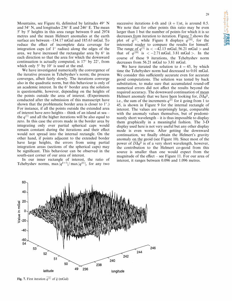
successive iterations k-th and �k � 1�st, is around 0.5.We note that for other points this ratio may be evenlarger than 1 but the number of points for which it is sodecreases from iteration to iteration. Figure 7 shows theplot of q�1�, while Figure 8 displays q�10�, for theinterested reader to compare the results for himself.The range of q�1� is < ÿ42:13 mGal; 56:21 mGal > andthat of q�10� is < ÿ2:71 mGal; 3:81 mGal >. In thecourse of these 9 iterations, the Tchebyshev normdecreases from 56.21 mGal to 3.81 mGal.

We have iterated the solution to k � 45, by whichtime the Tchebyshev norm had decreased to 0.01 mGal.We consider this sufficiently accurate even for accurategeoid computations. The solution was tested by backsubstitution, to make sure that accumulated round-offnumerical errors did not affect the results beyond therequired accuracy. The downward continuation of meanHelmert anomaly that we have been looking for, DDgh,i.e., the sum of the increments q�k� for k going from 1 to45, is shown in Figure 9 for the internal rectangle ofinterest. The values are surprisingly large, comparablewith the anomaly values themselves, but of predomi-nantly short wavelength – it is thus impossible to displaythem graphically in a meaningful fashion. The 3-Ddisplay used here is not very useful but any other displaymode is even worse. After getting the downwardcontinuation, we finally obtain the Helmert’s gravityanomaly on the geoid (see Figure 10). Since most of thepower of DDgh is of a very short wavelength, however,the contribution to the Helmert co-geoid from thissource is smaller than one would expect from themagnitude of the effect – see Figure 11. For our area ofinterest, it ranges between 0.096 and 1.096 metres.

Fig. 7. First iteration q�1� of q (mGal)

29

7. Conclusions

We had set out to investigate a specific question as towhether mean Helmert’s anomalies on the geoid can bederived from known mean Helmert’s anomalies at thesurface of the earth. In other words, we wanted toestablish if the so called ‘‘downward continuation’’ ofmean Helmert’s anomalies can be computed or not. Ourchoice of mean anomalies was dictated by a practicalconsideration stemming from the realization that mean

anomalies are the boundary values used in practice forsolving the geodetic boundary value problem. Ourchoice of Helmert’s anomalies came from the fact that:1) Helmert’s disturbing potential is harmonic outside thegeoid and thus also between the geoid and the earthsurface; 2) Helmert’s gravity anomalies at the earthsurface are by their nature smoother than the standardfree-air anomalies. We had also decided to use meananomalies for 50 by 50 geographical cells, because thesewere the ones we had readily at our disposal.

Fig. 8. Tenth iteration q�10� of q (mGal)

Fig. 9. Downward continuation DDgh

of 50 � 50 mean Helmert’s gravity anomalies (mGal)

30

We have selected a particularly rugged part ofCanada, the Rocky Mountains, in which to carry outour experiment. The reason for this choice should beobvious: if it turns out that the downward continuationcan be computed in the Rockies, with mountains over4,000 metres high, then there should be little troublecomputing it anywhere else in the world, with perhapsthe exception of the Himalayas.

When working with the Poisson problem, much likeworking with the Newton and Stokes problems, (i.e., theevaluation of the gravitational potential from Newton’sintegral and the evaluation of the geoid from Stokes’sintegral), one is supposed to evaluate a surfaceconvolution integral over the whole earth, which is animpractical requirement. We have overcome this tech-nical difficulty in much the same way as we overcome itin solving the other two problems, by splitting theintegration area into a small spherical cap – we havechosen a cap of radius equal to 1 arc-degree – aroundthe point of interest and the rest of the world. Thecontribution from the rest of the world is sufficientlysmall so that it can be evaluated to a sufficient accuracyusing one of the existing global gravity models. Tominimize this contribution further we also subtract thelow degree and order field – to degree and order 20, hasbeen our choice – from the observed mean Helmert’sanomalies at the earth surface and downward continuethis long wavelength part separately. Both thesecontributions (corrections) are evaluated in the spectraldomain from the global model GFZ93a and added to

the downward continuation of the higher degree andorder – above 20 – mean Helmert’s anomalies.

It turns out that the downward continuation of thehigher degree and order mean Helmert’s anomalies canbe obtained in a fairly simple manner. For our 17� by 22�

experimental area and the 50 by 50 mean anomalies, thePoisson integral equation is represented by 53,856 linearalgebraic equations. We have evaluated the conditionnumber for the corresponding matrix assembled forpoint values, rather than mean values. It is equal to 2,showing that the matrix is very well conditioned. (Ourmatrix, assembled for mean values, is probably some-what less well conditioned, judging from the number ofiterations needed.) There is thus no theoretical problemwith getting the inverse of this matrix.

Because the size of the matrix is daunting, we hadelected to solve the system by a simple iterative scheme.Table 1 shows how the iterations converge – to savespace, only every 5th iteration is shown – in bothTchebyshev’s and quadratic norms. It took 45 iterationsto get the Tchebyshev norm under 10 lGal, i.e., to makesure that the downward continuation is accurate to atleast 10 lGal for all the points in the area of interest.Interestingly, the quadratic norm of the iterated ‘‘meandifferences’’ q decreases by almost 9 orders of magnitudein the course of the 45 iterations. Some 22 iterationswould have sufficed if the mean threshold value of10 lGal were used.

For physical reasons unknown to us the effect of thedownward continuation of Helmert’s anomalies (i.e., of

Fig. 10. Helmert mean gravity anomaly �Dghg� on the geoid (mGal)

31

the difference between mean Helmert’s anomalies on theearth surface and on the geoid) on Helmert’s co-geoid(Vanicek and Martinec 1994) is everywhere positive –see Fig. 11. This is caused, mathematically, by the slightpositive long wavelength bias of the downward con-tinuation term. The high frequency variations of thedownward continuation do not seem to have much of an

effect on the co-geoid as Stokes’s integration effectivelydampens high frequency contributions.

We can thus claim that we have demonstrated thatmean Helmert’s anomalies can be successfully trans-ferred from the surface of the earth to the geoid, i.e.,that the downward continuation of mean Helmert’sanomalies on a 50 by 50 grid is a well posed and thereforesolvable problem. The natural smoothing (regulariza-tion) introduced by averaging the anomalies and thePoisson kernel over 50 by 50 (and possibly even muchsmaller) geographical cells is efficient enough toguarantee a unique solution of the downward continua-tion problem. Since in practical applications only meananomalies rather than point anomalies are used, webelieve that our results should put to rest the pervasiveuneasiness about the solvability of the downwardcontinuation problem. To be sure, there are still sometheoretical questions to be worked out, such as: Forwhat size of averaging cells will the solution show signsof breaking down, if at all? For what heights (averagedover the geographical cells) will the solution becomeunstable, if at all? Can a similar process be used for the

Fig. 11. Contribution to the Helmert co-geoid from the downward continuation of Helmert anomalies (m). Contour interval = 0.1 m

Table 1 Ranges and norms for every 5th iteration

n Range of the effect Tcheby. norm quadratic normPn

i�1 q�i� mGal of q�n� mGal of q�n� mGal2

1 () 42.13, 56.21) 56.21 0.2994E+25 () 94.60, 146.05) 13.49 0.5457E+010 ()118.68, 179.23) 3.81 0.2598E)115 ()124.99 189.09) 1.17 0.2187E)220 ()126.79, 192.16) 0.44 0.2566E)325 ()127.32, 193.13) 0.20 0.3853E)430 ()127.49, 193.44) 0.10 0.7013E)535 ()127.55 193.54) 0.05 0.1477E)540 ()127.56, 193.58) 0.03 0.3448E)645 ()127.57, 193.59) 0.01 0.8619E)7

32

downward continuation of mean free-air anomaliesencountered in Molodenskij’s approach and under whatcircumstances? How good is the Pellinen approxima-tion, which is normally used in the Molodenskijapproach? But these questions are, of course, beyondthe scope of this paper.

Acknowledgements. The research described in this contribution hasbeen supported by an NSERC of Canada operating grant to thesenior author and by a DSS contract with the Federal Governmentof Canada, Geodetic Survey Division (GSD) in Ottawa, let to theUniversity of New Brunswick; we wish to thank Mr. M. Veronneauof the GSD for providing us with all the data used here. We wish toacknowledge that Dr. Martinec’s stay in Canada, during the earlystages of this research was supported by an NSERC grant forInternational Scientific Exchange, while Dr. Sun’s presence on ourteam has been made possible by an NSERC InternationalFellowship grant. The senior author wishes to thank Dr. M.Vermeer for inspiring discussions conducted when he visited theFinnish Geodetic Institute earlier in 1994. Prof. Wm. R. Knight,UNB department of Mathematics and Statistics and department ofComputer Science, gave us some useful hints for solving our largesystem of equations. Thorough reviews of the earlier versions of themanuscript by M. Vermeer and 2 anonymous reviewers led to aconsiderable improvement of the manuscript. The authors are trulygrateful for the reviewers’ effort.

Appendix: Low frequency contributionand truncation error

To estimate the truncation error of the downwardcontinuation of gravity anomalies, we split the gravityanomaly on the geoid into two parts: low frequency part�Dgh

g�L and high frequency part �Dghg�

L:

Dghg � �Dgh

g�L � �Dghg�

L: �32�

Eqn. (11) can then be written as

Dght �

R4pr

Z

X0

DghgK�r;w;R�dX0

� DgL �R

4pr

Z

X0

�Dghg�

LK�r;w;R�dX0;

�33�

where

DgL �

R4pr

Z

X0

�Dghg�LK�r;w;R�dX0

�34�

is the low frequency part of gravity anomaly on theearth surface which can be calculated from a globalgravity model. To transform eqn. (34) into spectralform, we use the following expression for gravityanomaly as obtained from a global Helmert’s potentialmodel Th

jm

Dghg�X� � c

X1

j�2

�j ÿ 1�Xj

m�ÿj

ThjmYjm�X� �35�

and the orthogonality relations

4p2j � 1

Xj

m�ÿj

Y �

jm�X0�Yjm�X� � Pj�cosw�; �36�

Z

XY �

j1m1�X�Yj2m2�X�dX � dj1j2dm1m2 : �37�

Since the first term on the right hand side of eqn. (32)can be obtained from eqn. (35) as

�Dghg�L � c

XL

j�2

�j ÿ 1�Xj

m�ÿj

ThjmYjm�X�; �38�

the low frequency contribution DgL becomes

DgL �

Rc4pr

Z

X0

XL

ji�2

Xj1

m1�ÿj1

�j1 ÿ 1�Thj1m1

Yj1m1�X0�

�

X1

j2�0

�2j2 � 1�Rr

� �j2�1

�

4p2j2 � 1

Xj2

m2�ÿj2

Y �

j2m2�X0

�Yj2m2�X�dX0

� cXL

j�2

�j ÿ 1�Rr

� �j�2 Xj

m�ÿj

ThjmYjm�X�: �39�

The integration in the second term on the right handside of eqn. (33) can be truncated at spherical cap C0 sothat

R4pr

Z

X0

�Dghg�

LK�r;w;R�dX0

� �

R4pr

Z

C0

�Dghg�

LKm�H ;w;w0�dX0

�

R4pr

Z

X0ÿC0

�Dghg�

LKm�H ;w;w0�dX0

�

R4pr

Z

X0

�Dghg�

L�K ÿ Km

�dX0; �40�

where

Km�H ;w;w0� �K�H ;w�

ÿ

XL

j�0

2j � 12

tj�H ;w0�Pj�cos w� �41�

is the modified Poisson kernel with unknown coefficientstj. The second term on the right hand side of eqn. (41) isthe truncation error DgT to be minimized following theMolodenskij technique to minimize potential errorscoming from the employed global model. The thirdterm on the right hand side of eqn. (41) is equal to zero,because �Dgh

g�L is the high frequency �j > L� part of

gravity anomaly and �K ÿ Km� contains only the low

frequencies �j � L�. To get the unknown tj’s, we useSchwarz’s inequality:

33

Dg2T �

R4pr

Z

X0ÿC0

�Dghg�

LKm�H ;w;w0�dX0

� �2

<

R4pr

� �2Z

X0ÿC0

�Km�H ;w;w0��

2dX0

�

Z

X0ÿC0

��Dghg��

L�2dX0

: �42�

To minimize the upper bound of jDgT j we have tominimize

R

X0ÿC0

�Km�H ;w;w0��

2dX0, i.e.,

@

@tj

Z p

w0

Z 2p

0�Km

�H ;w;w0��2sin wdwda

� 2p@

@tj

Z p

w0

�Km�H ;w;w0��

2sinwdw � 0: �43�

Then the coefficients tj can be obtained from thefollowing system of equations:

XL

j�0

2j � 12

tj�H ;w0�eij�w0� � Qi�H ;w0�;

i � 0; 1; � � � ; L;

�44�

where

eij�w0� �

Z p

w0

Pi�cos w�Pj�cos w�sin wdw;

Qj�H ;w0� �

Z p

w0

K�H ;w�Pj�cos w�sin wdw :

�45�

Writing the modified Poisson kernel in a spectralform

Km�H ;w;w0� �

X1

j�0

2j � 12

Qj�H ;w0�Pj�cos w�; �46�

where

Qj�H ;w0� �

Z p

w0

Km�H ;w;w0�Pj�cos w�sin wdw; �47�

we obtain the truncation error DgT as

DgT �X� �

Rc4pr

Z

X0

X1

j1�2

Xj1

m1�ÿj1

�j1 ÿ 1�Thj1m1

Yj1m1�X0�

�

X1

j2�0

2j2 � 12

Qj2�H ;w0�

�

4p2j2 � 1

Xj2

m2�ÿj2

Y �

j2m2�X0

�Yj2m2�X�dX0

�

Rc2r

X1

j�2

�j ÿ 1�Qj�H ;w0�

�

Xj

m�ÿj

ThjmYjm�X�: �48�

Finally, eqn. (33) can be rewritten as

Dght �

R4pr

Z

C0

�Dghg�

LKm�H ;w;w0�dX0

� Dg1; �49�

where

Dg1 � DgL � DgT �50�

is the term to be used in eqns. (22)–(29) in the text. Wenote that it is only the higher frequency part of Dgh

g, i.e.,�Dgh

g�L, that is used in the solution of the Poisson

integral equation.

References

Bjerhammar, A., 1962, Gravity reduction to a spherical surface,Report of the Royal Institute of Technology, Geodesy Division,Stockholm.

Bjerhammar, A., 1976, A Dirac approach to physical geodesy,Zeitschrift fur Vermessungswesen, 101,41–44.

Forsberg, R., 1984, Gravity field terrain effect computations byFFT, Bull. Geod. 59, 342–360.

Gruber, T. and M. Anzenhofer, 1993, The GFZ 360 gravity fieldmodel, the European geoid determination, Proceedings ofsession G3, European Geophysical Society XVIII GeneralAssembly, Wiesbaden, May 3–7, 1993, published by thegeodetic division of KMS, Copenhagen. Eds. R. Forsberg andH. Denker.

Heiskanen, W.H., and H. Moritz, 1967, Physical Geodesy, W.H.Freeman and Co., San Francisco.

Kellogg, O.D. 1929, Foundations of Potential Theory. Springer,Berlin (reprinted 1967).

MacMillan, W.D., 1930, The Theory of the Potential. Doverreprint, 1958.

Martinec, Z. and P. Vanıcek, 1994, Direct topographical effect ofHelmert’s condensation for a spherical approximation of thegeoid, Manuscripta Geodaetica, 19, 257–268.

Molodenskij, M.S., V.F. Eremeev and M.I. Yurkina, 1960,Methods for Study of the External Gravitational Field andFigure of the Earth, English translation by Israel Programmefor Scientific Translations, Jerusalem, for Office of TechnicalServices, Department of Commerce, Washington, D.C., 1962.

Moritz, H., 1980, Advanced Physical Geodesy, H. WichmannVerlag, Karlsruhe.

Sjoberg, L.E., 1984, Least squares modification of Stokes’ andVening Meinesz’ formulas by accounting for truncation andpotential coefficient errors, Manuscripta Geodaetica, 9, 209–229.

Vanıcek, P. and E.J. Krakiwsky, 1986, Geodesy: the concepts, (2ndcorrected edition), North Holland, Amsterdam.

Vanıcek, P. and A. Kleusberg, 1987, The Canadian geoid –Stokesian approach, Manuscripta Geodaetica, 12, 86–98.

Vanıcek, P. and L.E. Sjoberg, 1991, Reformulation of Stokes’sTheory for Higher than Second-Degree Reference Field anda Modification of Integration Kernels, JGR 96 (B4), 6529–6539.

Vanıcek, P. and Z. Martinec, 1994, The Stokes-Helmert Schemefor the Evaluation of a Precise Geoid, Manuscripta Geodaetica,19, 119–128.

Wichiencharoen, C., 1982, The indirect effects on the computationof geoid undulations, Department of Geodetic Science, Rep.#336, Ohio State University, Columbus, Ohio, USA.

34