Introduction to Gravity Exploration Method
215
INTRODUCTION TO GRAVITY EXPLORATION METHOD First Edition Hamid N. Alsadi Former expert in Geophysics at Oil exploration Company, Iraq. Ezzadin N. Baban Professor in Geophysics at Department of Geology, University of Sulaimani. Sulaimaniyah, Kurdistan Region, Iraq, 2014 Kurdistan Region - Iraq Ministry of Higher Education and Scientific Research University of Sulaimani Faculty of science & Science Educations School of Science Department of Geology
-
Upload
sulaimaniu -
Category
Documents
-
view
0 -
download
0
Transcript of Introduction to Gravity Exploration Method

INTRODUCTION TO
GRAVITY EXPLORATION METHOD
First Edition
Hamid N. Alsadi Former expert in Geophysics at Oil exploration Company, Iraq.
Ezzadin N. Baban Professor in Geophysics at Department of Geology, University of Sulaimani.
Sulaimaniyah, Kurdistan Region, Iraq, 2014
Kurdistan Region - Iraq
Ministry of Higher Education and Scientific Research
University of Sulaimani
Faculty of science & Science Educations School of Science
Department of Geology

II
Copyright 2014 by Hamid N. Al-Saadi and Ezzadin N. Baban.
First Edition published 2014 by University of Sulaimani, Sulaimaniyah,
Kurdistan Region- Iraq.
Printed by Paiwand press, July 2014, Sulaimaniyah, Kurdistan Region, Iraq.
This work is subject to copyright. All Rights Reserved.
No part of this publication may be reproduced, stored in a retrieval system,
or transmitted, in any form or by any means, electronic, mechanical,
photocopying, recording, scanning or otherwise, without the permission in
writing of the publisher and the copyright owner.
Bibliography:
Includes index
Exploration- Gravity method
Hamid N. Al-Saadi and Ezzadin N. Baban
III
Content
PREFACE ..................................................................................................................... ix
ACKNOWLEDGMENT ............................................................................................. x
Chapter 1
INTRODUCTION ....................................................................................................... 1
2.1. General Review ............................................................................................ 1
2.2. Historical Review ......................................................................................... 2
2.3. The Earth Shape ........................................................................................... 4
1.3.1 The Ellipsoid ................................................................................................ 4
1.3.2 The Geoid ................................................................................................... 5
Chapter 2
THE EARTH GRAVITATIONAL FIELD ............................................................. 7
2.1. The Universal Law of Gravitation ........................................................ 7
2.2. The Gravitational Acceleration ............................................................ 8
2.3. Gravity Computations of Large Bodies ................................................ 9
2.4. The Acceleration Unit ........................................................................10
2.5. Gravity Gradients ...............................................................................11
2.6. Gravitational Field Intensity and Potential ........................................12
2.7. Concept of the Equipotential Surface ...............................................13
2.8. The Earth Gravity Variations..............................................................14
Chapter 3
THE GLOBAL GRAVITY VARIATIONS .......................................................... 17
3.1. The Shape Effect ........................................................................................17
3.2. The Rotation Effect ....................................................................................19
3.3. The Combined Effect .................................................................................19
3.4. Normal Gravity ..........................................................................................21

IV
Chapter 4
THE LOCAL GRAVITY VARIATIONS ............................................................. 23
4.1. Elevation Effect ..........................................................................................23
4.2. Excess-Mass Effect .....................................................................................25
4.3. The Topographic Effect ..............................................................................26
4.4. Geological Effects ......................................................................................26
4.5. Time-Variant Changes ...............................................................................27
Chapter 5
GRAVITY MEASUREMENTS ............................................................................. 29
5.1. Features of Gravity Measuring Instruments .............................................29
5.2. Methods of Measuring Gravity .................................................................30
5.2.1 Free-falling ................................................................................................30
5.2.2 Swinging Pendulum ..................................................................................31
5.2.3 Spring Gravimeter ....................................................................................33
5.3. Instrument Calibration ..............................................................................43
5.4. Instrumental Drift ......................................................................................43
Chapter 6
GRAVITY FIELD SURVEYING ........................................................................... 45
6.1. Land Gravity Surveying ..............................................................................45
6.1.1 The Gravity Field Data ..............................................................................45
6.1.2 The Base-station network ........................................................................46
6.1.3 The Survey Gravity Readings ....................................................................48
6.1.4 Station Locations and Elevations ..............................................................49
6.2. Marine Gravity Surveying ..........................................................................49
6.2.1 Sea-Floor Measurements .........................................................................50
6.2.2 Shipboard Measurements ........................................................................50
6.2.3 Eotvos Correction .....................................................................................51
6.3. Airborne Gravity Surveying .......................................................................53

V
6.4. Microgravity Surveying ..............................................................................54
Chapter 7
GRAVITY DATA PROCESSING ......................................................................... 55
7.1. Instrument Calibration and Drift Correction .............................................56
7.2. Latitude Correction ....................................................................................56
7.2.1 Rate of Change of Normal Gravity ............................................................57
7.3. Elevation Corrections ................................................................................59
7.3.1 Free-air Correction (FAC) ..........................................................................59
7.3.2 Bouguer Correction (BC) ...........................................................................60
7.3.3 Terrain Correction (TC) .............................................................................61
7.4. Isostatic Correction....................................................................................66
7.5. Data Reduction of Marine Gravity Data ....................................................67
7.5.1 Reduction of Shipboard Gravity Data .......................................................68
7.5.2 Reduction of Sea-Floor Gravity Data ........................................................69
7.6. Accuracy of Bouguer Gravity Data.............................................................69
Chapter 8
THE GRAVITY ANOMALY .................................................................................. 73
8.1. Concept of the Gravity Anomaly ...............................................................73
8.2. Computation of Gravity Anomalies ...........................................................74
8.3. Spherical Shapes ........................................................................................75
8.3.1 Point Mass ................................................................................................75
8.3.2 Spherical Shell...........................................................................................75
8.3.3 Solid Sphere ..............................................................................................77
8.4. Cylindrical Shapes ......................................................................................80
8.4.1 Horizontal Line Mass ................................................................................80
8.4.2 Horizontal Cylinder ...................................................................................81
8.4.3 Vertical Line Mass .....................................................................................84

VI
8.4.4 Vertical Cylinder .......................................................................................85
8.5. Sheets and Slabs ........................................................................................90
8.5.1 Horizontal Sheet .......................................................................................90
8.5.2 Horizontal Thin Slabs ................................................................................92
8.5.3 Horizontal Thick Slab ................................................................................92
8.6. Rectangular Parallelepiped........................................................................95
8.7. Bodies of Irregular Shapes .........................................................................96
8.7.1 Two-Dimensional Models .........................................................................97
8.7.2 Three-Dimensional Models ......................................................................99
Chapter 9
INTERPRETATION OF GRAVITY ANOMALIES ....................................... 101
9.1. Scope and Objective ................................................................................101
9.2. Role of Rock Density ................................................................................102
9.2.1 Densitiy Variations ..................................................................................103
9.2.2 Ranges of Rock Densities ........................................................................104
9.2.3 Density Determination Methods ............................................................107
9.3. Ambiguity in Gravity Interpretation ........................................................111
9.4. The Direct and Inverse Problems ............................................................111
9.5. Regional and Residual Gravity .................................................................113
9.6. Anomaly Separation Schemes .................................................................114
9.6.1 The Graphical Approach .........................................................................114
9.6.2 The Analytical Approach .........................................................................116
9.7. Interpretation Techniques .......................................................................128
9-7-1 Trial-and-Error model analysis ...............................................................128
9-7-2 Inversion Model Analysis .......................................................................131
Chapter 10
CRUSTAL STUDIES AND ISOSTASY ............................................................ 141
10.1. The Structural Model of the Earth .......................................................141

VII
10.2. The Structural Model of the Crust .......................................................142
10.3. Role of Gravity Data in Crustal Studies ................................................143
10.4. Concept of Isostasy ..............................................................................145
10.5. Isostasy-Density Relationship ..............................................................146
10.6. Hypotheses of Isostacy ........................................................................147
10.5.1 Pratt’s Hypothesis .................................................................................148
10.5.2 Airy’s Hypothesis ..................................................................................149
10.7. Modifications to the Isostatic Models ................................................150
10.8. The Isostatic Correction .......................................................................151
10.9. The Isostatic Anomaly .........................................................................152
10.10. State of Isostatic Compensation ..........................................................153
10.11. Deviations from Isostatic Equilibrium .................................................155
10.12. Testing for Isostatic Equilibrium ..........................................................155
10.13. Isostatic Rebound Phenomenon .........................................................156
10.14. Examples of Isostatic Deviation ...........................................................157
10.13.1 Gulf of Bothnia ...................................................................................157
10.13.2 Rift Valleys ..........................................................................................158
10.13.3 The Red Sea ........................................................................................159
10.13.4 Ocean Deeps and Island Arcs .............................................................159
10.13.5 Cyprus and Hawaii Islands ..................................................................160
Chapter 11
GRAVITY EXPLORATION RECENT DEVELOPMENTS ......................... 161
11.1. Airborne Gravity ..................................................................................161
11.1.1 Aerogravity Basic Principles .................................................................162
11.1.2 Aerogravity Main Objectives ................................................................163
11.1.3 Historical Development of Aerogravity ...............................................164
11.1.4 Advantages and Limitations of Airborne Gravimetry ...........................165
11.1.5 Accuracy and Spatial Resolution of Airborne Gravimetry ....................166
11.1.6 Processing of the Aerogravity Data ......................................................166

VIII
11.2. Borehole Gravity ..................................................................................169
11.2.1 Principles of Borehole Gravity ..............................................................169
11.2.2 Operational Considerations ..................................................................169
11.2.3 Advantages and Disadvantages of Borehole Gravity ...........................170
11.2.4 Scope of Applications ...........................................................................170
Chapter 12
CASE HISTORY OF GRAVITY SURVEYS ..................................................... 171
REFERENCES ........................................................................................................ 193
INDEX ....................................................................................................................... 199

IX
PREFACE This book is written mainly for university students taking a course on gravity as
one of the methods used in geophysical exploration. It is designed to be an
introductory text book that deals with the basic concepts underlying the
application of the Earth gravitational field in the exploration of the subsurface
geological changes and in prospecting of petroleum and other mineral deposits.
As it is familiar with the exploration geophysicists, this subject is fully dealt with
in many original authentic internationally-known text books. In this publication,
no new subjects were added to those found in the other standard books which are
well known in the geophysical library. In fact these and other related scientific
papers and research reports formed the solid references for the present work.
There is, however, a difference in the design and presentation approach. The
essential publications, used as references, are listed at the end of the book. The
main feature of this work is being concise and logically sequenced. The
objective was to present the subject in a simple and clear way avoiding excessive
descriptions and unnecessary lengthy comments. For this reason the text was
provided with numerous illustration figures for extra clarification.
The book consists of twelve chapters. The first five chapters cover the theoretical
aspect of the subject including the gravitational attraction, shape of the planet
Earth and nature of the gravity variations, which forms the basis for the
exploration capability of the method. The following five chapters deal with
measuring instruments, field surveying techniques, data processing, concept of
the gravity anomaly and interpretation. A closely associated with gravity
anomaly is the phenomenon of isostasy. This was presented in chapter 10. Some
modern aspects of the method were covered in chapter 11 and in the last chapter
12 actual gravity field-surveys were reviewed. The first case history is an actual
field survey conducted by one of the authors (Hamid Alsadi) in the south-west
England in 1965-1966 and the others (by Zuhair Al-Sheikh and Ezzadin N.
Baban) were carried out in Iraqi territories. These are included here to serve the
purpose of showing how a real gravity surveying is carried out in practice under
actual field and processing environments.
As always in any publication material, there is always a room for improvement if
extra time and effort has been allocated. From personal experience this is an
endless process. However, this book is no exception to this rule. With feed-backs
from future users of the book it is hoped to make the improvement changes
needed that will be incorporated in future editions.
Hamid N. Alsadi and Ezzadin N. Baban,
23 Jan. 2013

X
ACKNOWLEDGMENT
We would like to express my gratitude to the all people who support, offered
comments, evaluation and assisted in the editing, proofreading and design saw us
through this book;
We would like to thank professors Dr. Bakhtiar Kadir Aziz and Dr. Ali
Mahmood Surdashi for their scientific evaluation and Mr Ari Mohammed
Abdulrahman for language’s evaluation and their feedback on this book.
We wish to extend our sincere thanks to Professor Dr. Hamid Majid Ahmed
head of the Central Committee for books approving and publishing at Sulaimani
University for invaluable help, comments and approving in preparation of the
book.
We would like to thank Presidency of Sulaimani University, Faculty of Science
and Education Sciences, School of Science and Geology Department for
enabling us to publish this book.

Chapter 1
INTRODUCTION
2.1. General Review
The basic concept underlying gravity surveying is the variation of the Earth
gravitational field caused by lateral variation of subsurface rock-densities. In
other words, a given rock body whose density is different from its surrounding
medium (i.e. geological anomaly) produces a corresponding disturbance (gravity
anomaly) in the Earth gravity-filed. The form and amplitude of the created
anomaly depend on the subsurface geological anomaly such as a salt dome,
granite intrusion, buried valley, folded or faulted beds. The gravity anomaly
depends also upon large scale or regional structures such as regional dipping
strata, sedimentary basins, geosynclines and mountain roots
Gravity surveying involves measurements of the changes in gravitational
acceleration at a grid of points over a given area. The observation-data are then
subjected to a series of corrections and mathematical analyses in order to reduce
them to gravity values measured relative to a defined datum-plane, normally
taken at the mean sea level. These corrections ensure that the produced gravity
anomaly is that caused by the sub sea-level geological anomaly with all other
effects removed.
In the last stage of the survey, the obtained gravity anomaly is subjected to
further analysis with the aim of determination of the causing subsurface
geological anomaly. This gravity-to-geology process (interpretation) forms the
ultimate objective of any gravity-survey project.

2
2.2. Historical Review
The historical development of gravity exploration may be summarized as
follows:
Late 16th and early 17th centuries:
Galileo Galilei (1564-1642) discovered, in about 1590, that objects of
different masses fall to Earth surface at same constant acceleration. Johannes
kepler (1571-1630) derived three laws (Kepler Laws) which describe the
motions of planets in the solar system. These laws were later used by the English
physicist, Sir Isaac Newton (1642-1727), in formulating the universal law of
gravitation, giving the mathematical expression (F=Gm1m2/r2) for the force of
attraction, F (gravitational force) that exists between any two masses, m1 and m2
which are located at r distance apart. The law was published in 1687.
18th century:
A pioneering work was done by the French scientist Pierre Bouguer (1698-
1758), who had led an expedition in (1735-45) organized by the French
Academy of Sciences to conduct gravitational studies and other investigations
concerning the shape of the Earth. He derived the relationships connecting
gravity variation with elevation and latitude. The Bouguer gravity anomaly is
named after his name.
19th century:
The main development that took place then was the introduction in 1817, by
the English physicist, Henry Kater (1777-1835), of the compound pendulum
known now by his name, Kater pendulum which was used in gravity
measurements during the following century. Also the Hungarian physicist,
Roland von Eotvos (1848-1919), completed the torsion balance in 1890 with
which the spatial derivative of the gravity changes can be measured.
First half of the 20th century:
The first application of the torsion balance was made in gravity surveying
over an ice sheet of a lake in 1901 and the first torsion-balance survey for oil
3 Chapter 2 : Introduction
exploration (in California and Texas) was conducted in 1922. The portable
pendulum began to be used in the early 1920s. It (the pendulum) was used by F.
A. Vening Meinesz in 1923 in gravity measurements on board of submarine to
study the gravity variations over some oceanic areas.
Gravimeters were introduced and utilized in the search for oil and minerals.
In 1932, the gravimeter (stable type) was introduced as an exploration tool, and
in 1939, the LaCoste gravimeter (zero-length spring) appeared. In 1948, the
Worden and Atlas gravimeters, as improved portable instruments, became in
common use for gravity field-measurements.
Second half of the 20th century:
During the second half of the twentieth century, the gravity techniques have,
like other branches of science and technology, witnessed appreciable advances.
During the period 1940-1960, the techniques of mathematical computation of
gravity anomalies of simple geometrical shapes were developed. In the few years
around 1960, George Woollard (1908-1978) used Pendulum measurements to
establish a world-wide network of gravity base-stations. The digital computers
introduced in the 1960’s have facilitated gravity data processing and
interpretation capabilities. In particular, digital filtering by Fourier Transform,
model analysis and inversion techniques were applied in the analysis and
interpretation of gravity data.
In this period, gravimeters have been adopted to measurements in boreholes,
on sea-floors, on moving ships, and on aircrafts (La Fehr, 1980). Satellite orbital
paths furnished valuable knowledge on the detailed shape of the Earth (Kahn,
1983).
The Recent Developments
The main recent development that occurred in the gravity exploration
method was the practical application of the airborne gravity as an effective
exploration tool (Elieff, 2003; Hwang, et al, 2007; Alberts, 2009).
Satellite radar-based positioning technique, computer hardware, and
software systems and all other modern supporting technologies (based
principally on modern digital electronics) have collectively contributed to the
recent developments of the gravity method.

4
2.3. The Earth Shape
1.3.1 The Ellipsoid
The past geodetic and geophysical investigations coupled with the more
recent satellite data led to the conclusion that the Earth is approximately
ellipsoidal rather than being perfectly spherical. The model which is now
adopted for the Earth shape, is an ellipsoid of revolution whose surface is taken
to be the mean sea-level surface of the Earth. This model is called the reference
or normal ellipsoid. It is sometimes called the reference spheroid (Fig. 1-1).
In 1930, dimensions of the agreed-upon normal ellipsoid were adopted by an
organization called the International Union of Geodesy and Geophysics (IUGG).
By 1967, the numerical constants of the ellipsoidal model were updated to the
now- accepted values which are:
The equatorial radius (a) = 6378.160 km
The polar radius (b) = 6356.775 km
The difference (a-b) = 21.385 km
The flattening factor (a-b)/a = 1/298.25
The angular Rotation Speed (ω) = 7.292 * 10-5 radian/sec
a
Spheroid
Ellipsoid b
Fig. 1-1 The ellipsoidal model of the Earth

5 Chapter 2 : Introduction
1.3.2 The Geoid
In order to have a reference datum level to which measurements can be
related, a physical surface for the Planet Earth was defined. This surface is taken
to be the average sea-level over the oceans and over the sea-water if it were
extended in canals cut through the continents. This global surface is commonly
referred to as the geoid. The geoid surface is horizontal (i.e. perpendicular to
plumb line) at all its points (Fig. 1-2).
In general, the geoid surface does not coincide with that of the normal
ellipsoid. In fact, the deviation between the two surfaces can be as large as 100
meters. The reason for this discrepancy is that the geoid suffers from certain
surface deformations (geoid undulation) caused by small-scale and large-scale
density anomalies in the Earth crust.
A small-scale localized excess-mass anomaly would warp the geoid upward.
Under large-scale continental blocks, the geoid surface is warped upwards due to
rock material existing above it, and it is warped downwards over the oceans
because of the lower density of the water.
The geoid with its natural undulations presents a model closer to the actual
Earth than any other suggested models. It differs from the ellipsoid model which
is based upon a simplified theoretical Earth in which density is allowed to vary
vertically (with depth) but not laterally (Fig. 1-3).
Ellipsoid
b
a
Geoid
Fig. 1-2 The geoid with its undulations is defined by the mean sea-level.
The dotted line represents the Earth reference ellipsoid.

6
According to the geopotential concept, the undisturbed ocean surface is an
equipotential surface. This means that the geoid surface has, by definition, the
same gravitational potential as the mean ocean surface
The geoid surface is used as a reference (datum level) for local geodetic and
geophysical survey measurements. However, large-scale global measurements
(such as astronomical surveying) are made relative to the reference ellipsoid.
ρ1
ρ1
ρ2
ρ3
ρ3
ρ2
Fig. 1-3 Density distribution in the two models, the ellipsoid (A) and the geoid
(B) that are developed for the Earth.
(A) (B)

Chapter 2
THE EARTH GRAVITATIONAL FIELD
One of the principal potential fields existing in nature is the Earth
gravitational field. Within this field, a force of attraction occurs between any two
masses existing in universe. The basic physics has furnished mathematical laws
that govern the behavior of all the scalar and vector quantities associated with
this phenomenon. In this chapter, we shall present simple explanatory notes for
the scalar gravitational potential and for the gravitational vectors; force,
acceleration and gradients.
2.1. The Universal Law of Gravitation
Isaac Newton (1643-1727) formulated the universal law of gravitation which
evaluates the attraction force F that exists between two particles of masses m1
and m2 located at distance r apart (Fig. 2-1):
F = G m1 . m2 /r2
m1
m2
r
Fig. 2-1 Attraction force (F) between two masses; m1 and m2 at distance r
apart.

8
The constant G, called the Universal Gravitational Constant, was
experimentally determined and found to be of the value:
G = 6.673 10 8 (cm 3 .gm-1.sec-2)
or,
G = 6.673 10-11 (m 3 .kg-1.sec-2)
2.2. The Gravitational Acceleration
Newton's second law of motion states that any body of mass (m) under the
effect of force (F) moves with acceleration (a) where:
F = ma
Now, in the case of two particle-masses (m1 and m2), suppose one of them
(mass m2, say) is free to move, then this mass (m2), which is under the influence
of the attraction force due to the pull of the stationary mass m1, will move
towards m1 with acceleration a1.
By combining these two laws, equations 3-1 and 3-2 for the two-mass
system, the following relationship is readily obtained:
a1 = Gm1 / r2
Likewise, if m1 is the mass that is free to move, then it will move towards
the mass m2 with acceleration a2.
The acceleration a is directly proportional to the causing mass m and
inversely proportional to the square of the distance r. Thus, the vector quantity a,
which is the acceleration imposed, by a mass m, on a number of masses (m1, m2,
…) located at the same distance from m, will be the same regardless of their
individual masses (Fig. 2-2).

9 Chapter 2 : The earth gravitational field
2.3. Gravity Computations of Large Bodies
Equation 3-3 expresses the relationship between a particle-mass
(infinitesimal body) and the acceleration created at a point located at a defined
distance from it. A particle of mass Δm would create an acceleration Δg at an
observation point at r distance away is given by:
Δg = G Δm / r2
In gravity surveying work, two modifications need to be introduced. The
first is that the acceleration measured or computed is the vertical component, and
the second modification is that the gravity source is a finite body-mass and not
an infinitesimal particle. This is necessary since, in practice, all survey activities
are concerning large mass-bodies buried at certain depths below ground surface.
The approach (Fig. 2-3) for the computation of the vertical component of
acceleration (gz) for a mass-body of finite size is by considering the body as
being consisting of a large number of particles and then computing the vector
sum of the contributions (Δgz) of the constituent particles. For the nth particle
(Δmn) of a body buried at depth below the surface, the vertical component of its
acceleration (Δgn) at the observation point (P, Fig. 2-3) is given by:
Δgn = (G Δmn / rn2) cos θn
Fig. 2-2 Acceleration vectors (a) indicated by red arrows are due to the attraction
force imposed by the mass (m) upon masses (m1, m2 ,… , m5) which are at equal
distances from the causing mass (m). Vectors (a1, a2, …) are of equal magnitudes
regardless of the magnitude of these attracted masses.
m
m1
m2
m3
m4
m5

10
The net vertical component of acceleration (gz) due to the whole body is
obtained by summing the effects of the individual particles of the body, that is
the sum Σ Δgn , where:
gz = G Σ ( Δmn / rn2) cos θn
Using Cartesian coordinate system for a three dimensional body of constant
density (ρ), this equation may be re-expressed by the integral form:
gz = G ρ ∫∫∫ z (x2 + y2 + z2 )-3/2 dx dy dz
It should be noted here that the term gravity is used in the geophysical
literature to mean gravitational acceleration.
2.4. The Acceleration Unit
Normally the acceleration is measured by units having (in the cgs system)
the dimensions of cm/sec2
. This is called the gal after the Italian physicist
Galileo. This unit is too large for practical survey measurements and thus the
Fig. 2-3 The approach for computing the vertical component of acceleration
caused by a mass-body of a finite size. Two-dimensional body (lamina) is used
here to clarify the concept.
z
x P
θ
Δmn
11 Chapter 2 : The earth gravitational field
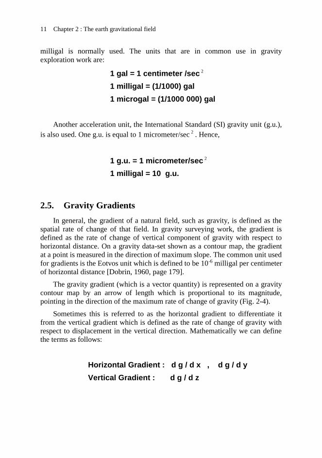
milligal is normally used. The units that are in common use in gravity
exploration work are:
1 gal = 1 centimeter /sec 2
1 milligal = (1/1000) gal
1 microgal = (1/1000 000) gal
Another acceleration unit, the International Standard (SI) gravity unit (g.u.),
is also used. One g.u. is equal to 1 micrometer/sec2
. Hence,
1 g.u. = 1 micrometer/sec 2
1 milligal = 10 g.u.
2.5. Gravity Gradients
In general, the gradient of a natural field, such as gravity, is defined as the
spatial rate of change of that field. In gravity surveying work, the gradient is
defined as the rate of change of vertical component of gravity with respect to
horizontal distance. On a gravity data-set shown as a contour map, the gradient
at a point is measured in the direction of maximum slope. The common unit used
for gradients is the Eotvos unit which is defined to be 10-6 milligal per centimeter
of horizontal distance [Dobrin, 1960, page 179].
The gravity gradient (which is a vector quantity) is represented on a gravity
contour map by an arrow of length which is proportional to its magnitude,
pointing in the direction of the maximum rate of change of gravity (Fig. 2-4).
Sometimes this is referred to as the horizontal gradient to differentiate it
from the vertical gradient which is defined as the rate of change of gravity with
respect to displacement in the vertical direction. Mathematically we can define
the terms as follows:
Horizontal Gradient : d g / d x , d g / d y
Vertical Gradient : d g / d z

12
2.6. Gravitational Field Intensity and Potential
In and around the Earth there exist a number of natural fields, such as the
magnetic, electric, and gravitational fields. Any of these fields is defined as
space in which the effect of force-source can be experienced. There are two main
parameters associated with the field. These are the field intensity (field strength)
and the field potential. Both of these parameters have measurable values at every
point in the space where the field exists.
It is to be noted here that the geophysical techniques applied in oil and
mineral explorations which utilize such natural fields (e.g. gravity, magnetic or
electric) are sometimes referred to as potential methods because they are all
having potential fields.
For the gravitational field, the field intensity at a given point is defined as
the force (or acceleration, g) a unit mass experiences when positioned at that
point. It is a vector quantity in the direction of the source of the field.
The second parameter is the potential of the gravity field (U). The
gravitational potential at a given point is defined as the work spent in moving a
unit mass from infinity to that point. Unlike the intensity, the potential is a scalar
quantity.
Fig. 2-4 Vector representation of the gravity gradient. Length of the
arrow is proportional to the magnitude of the gradient at the point of
measurement.
200 mgal
300 mgal
400 mgal

13 Chapter 2 : The earth gravitational field
By definition, the potential (U) at a point located at distance (r) from the
centre of the Earth (of mass M) is given by U(r) where,
U(r) = G M ∫(1/r2)dr
That is:
U(r) = - G M /r
Conversely, differentiating the function U(r) with respect to the distance (r)
gives the gravitational force (F), that is
F = dU/dr
Or:
F = G M /r2
This is the mathematical relationship between the two parameters, the scalar
(U) and the vector (F). It shows that the gravity force (F) or the acceleration (g)
at a point is proportional to the gradient of the potential (U) of the gravitational
field at that point.
The concept of potential can be used in gravity computations instead of the
gravity force or acceleration. The gravitational potential U(r) has the units of cm2
/ sec2.
2.7. Concept of the Equipotential Surface
The equipotential surface is defined as the surface existing within a potential
field on which the potential function U(r) is constant. This implies that there is
no force component acting long that surface. This also means that the force at
any point of the surface is always perpendicular to the equipotential surface at
that point.
Over a part of the Earth surface where the subsurface medium is
homogeneous, the gravitational equipotential surface of the gravity field will
have a curvature which is equal to that of the earth surface which locally appears
as horizontal to an observant. For the case of an anomalous mass existing below
surface, the equipotential surface shall warp in such a way as it becomes
perpendicular to the gravity direction (plumb line direction) at each of its points
(Fig 2-5). The warping is upward for a mass of surplus density and downward
for a deficient density.

14
The ocean surface (geoid surface) is in fact an equipotential surface. It is
horizontal surface in the sense that it is perpendicular to the plumb lines at all
points of the ocean surface.
2.8. The Earth Gravity Variations
As a matter of fact, the Earth gravitational field in space is not constant, but
varies from one point to another. There are several factors that bring about
gravity changes on and above the Earth surface. At an observation point, the
measured gravity force (or acceleration) represents the vector sum of the various
gravity components generated from different sources.
If the Earth were stationary, homogeneous and perfectly spherical in shape,
then the intensity of its gravitational field would have been of constant value
over its entire surface. In reality, however, the earth is not homogeneous and it is
neither stationary nor perfectly spherical. The earth is an ellipsoid of revolution
rotating about its polar axis. These two factors, in addition to the inhomogeneous
nature of the Earth crust, are the main causes for disturbing the uniformity of the
gravitational field.
The rotating flattened earth causes the gravity value to change according to
latitude position. Beside this uniform global variation of the earth gravity there is
another type of variations of local origins. The main cause for the local
(anomalous) gravity changes is the existence of lateral density variations found
Fig. 2-5 Effect of density variation on the generated equipotential surfaces;
(A) Case of no lateral density changes, (B) Case of an anomalous, surplus-
density body
(A) (B)
∞ ∞

15 Chapter 2 : The earth gravitational field
in the crust of the Earth. In fact, all local deviations in the Earth crust from the
uniform ellipsoidal-model would disturb the uniformity of the Earth gravitational
field. These detailed gravity changes that are of localized nature (caused by the
existence of anomalous geologic bodies) form the basis for oil and mineral
exploration by gravity surveying.
As shown in the following flowchart (Fig. 2-6), the Earth gravity-variations
may be subdivided into two main types. The first type is the global (general)
variation which is attributed to both rotation and flattening features of the earth.
This is expressed by a mathematical formula that describes what is called the
Normal Gravity of the Earth. Superimposed on this global type of variations, is
the local (detailed) variation caused by the geological and topographic
conditions prevailing in the neighborhood of any observation point used for the
measurement.
Fig. 2-6 Flowchart showing the two types of the Earth gravity variations; the
global and the local types of variations.
Local variations
Shape of Planet Earth
Rotation of Planet Earth
Gravity variations
Global variations
Space-Variant changes
terrain and geological effects
Time-Variant changes
tidal and instrumental-drift effects

16

Chapter 3
THE GLOBAL GRAVITY VARIATIONS
The earth is an ellipsoid of revolution rotating about its polar axis. These
two factors (ellipsoidal shape and rotation) disturb the uniformity of the global
gravitational field. Part of the effect is due to the Earth shape (shape effect) and
the other part is due to its rotation (rotation effect).
3.1. The Shape Effect
As we have presented in a previous discussion, the gravitational acceleration
(g), measured on the surface of a static homogeneous spherical Earth of mass M,
density ρ, and radius R, is given by:
g = G M / R2 = 4π G R3ρ/3R2
Hence,
g = 4π G R ρ/3
In this case, since R and ρ are constant, g will be constant all over the Earth
surface or over any other concentric spherical surface (Fig. 3-1).
R g
g
g
g
g
g
Fig. 3-1 Gravity field of a homogeneous spherical model of the Earth

18
In reality, the Earth is not a sphere but an ellipsoid of revolution with its
polar radius shorter than the equatorial radius by 21 km. In this case, the
distances of the surface-points vary from location to location and hence the
gravity value changes accordingly (Fig. 3-2).
The ellipsoidal shape of the Earth has the effect of increasing gravity as the
observation point gets nearer to the poles. In fact, the gravity value, measured at
any point on the mean sea level surface, is always higher than that measured at
the mean sea level surface at the equator. It reaches its maximum value at the
polar points (Fig. 3-3).
Fig. 3-2 Gravity field of a homogeneous ellipsoidal model of
the Earth.
b
g2
g1 a
g3
Fig. 3-3 Variation of the gravity vector (red arrows) over the
Earth surface due to its ellipsoidal shape. Length of arrow is
proportional to gravity magnitude.
g1
g2
g3

19 Chapter 3 : The global gravity variations
3.2. The Rotation Effect
A body on the surface of a rotating Earth experiences a centrifugal force that
acts in opposite direction to the gravitational attraction force. Because the Earth
is rotating about its polar axis, the developed centrifugal force attains its
maximum value at the equator where the rotation radius attains its maximum
length, rmax (Fig. 3-4).
The magnitude of the centrifugal acceleration of a body rotating at an
angular speed (ω) is equal to (ω2r), where r is the rotation radius. Thus, the
gravity-vector contributed due to rotation is maximum at the equator decreasing
gradually towards the poles (Fig. 3-5). It reaches zero-value at the polar points.
The reason for the change is that the rotation radius becomes less as the rotation
plane of a point at the earth surface gets nearer to the poles.
Development of the centrifugal force and the manner of its variation seem to
give the logical explanation for the cause of the flattening phenomenon of the
Earth. Accordingly, the flattening process is therefore, expected to continue with
time bringing further flattening in the future.
3.3. The Combined Effect
Because the Earth is ellipsoidal and rotating about its shorter (polar) axis,
its actual gravity is made up of the two vectors; the gravitational attraction
directed towards the Earth centre and the opposing centrifugal force in the
direction perpendicular to the polar axis (Fig. 3-6).
rmax
r
r
Fig. 3-4 Change of the rotation radius (r) with the location on the
Earth surface.

20
The measured acceleration vector at each point on the Earth surface is the
resultant (i.e. combined effect) of two components acting at that point. These are
the gravitational attraction of the Earth-mass and the centrifugal force due to the
Earth-rotation.
The gravity has its maximum value at the Equator and its minimum value at
the polar points. In fact, the observed gravity value at the poles exceeds that at
the equator by about 5200 mgal. This difference is found to be about half the
value expected from shape considerations only. The reduction is interpreted to
be caused by the subsurface mass in the equatorial bulge which creates an extra
gravity component that increases the equatorial value, giving the difference of
5180 (i.e. about 5200) mgal.
Fig. 3-5 Variation of the gravity-vector over the Earth surface due to
Earth rotation.
g
gc
gE
Fig. 3-6 Resultant gravity (g) of the two components; Earth-
mass gravity (gE) and centrifugal acceleration (gc).

21 Chapter 3 : The global gravity variations
It is worth noting that the net gravitational vector does not point to the
centre of the Earth except at the pole and at the equator. This is because at the
pole, there is only the mass effect (rotation effect is zero) and at the equator
where the two effects are collinear but in exactly opposite directions.
3.4. Normal Gravity
As it is mentioned above, the Earth reference-surface for gravity
computations is defined to be the surface of the ellipsoid which coincides with
the mean sea level. This is called the reference ellipsoid or the normal ellipsoid,
and the gravitational field determined over this surface is given the term Normal
Gravity.
The Normal Gravity (gN) is expressed as a mathematical function of latitude
(Φ), that is gN (Φ). It describes the global gravity variation which is attributed to
both of flattening and rotation of the Earth.
The first normal-ellipsoid model was defined in 1930 by the International
Union of Geodesy and Geophysics (IUGG). Based on the constants of this model
together with the measured gravity value at the equator, the first theoretical
formula for the Normal Gravity, gN(Φ), was formulated (see Nettleton, 1976,
p17). The measurements involved in the computations were adjusted to the
pendulum measurements made at the German city Potsdam in 1906. This
formula is normally referred to as the International Gravity Formula (IGF).
In 1963, the Society of Exploration Geophysicists (SEG) published the
results of a global gravity measurements by G.P. Woollard. The publication
includes the gravity values that were obtained from pendulum and gravimeter
measurements made at the worldwide network of observation stations, (now
called the International Gravity Standardization Net, 1971, IGSN71).
In about the year of 1965, accuracy of gravity measurements has largely
improved, attaining a tenth of the milligal. After this time, more accurate
measurements made by gravimeter and falling-mass methods revealed that the
Potsdam-based value is 14-mgal too high. In view of this finding the data
published by SEG in 1963 had to be corrected by subtracting 14 mgal.
In 1967, more accurate satellite data and more advanced measurement
technology led to revision by the IUGG of the normal ellipsoid model of the
Earth. The refined Normal Gravity formula based on this revised ellipsoid was
determined. This formula, which replaced the IGF, is called the 1967-Geodetic
Reference System (GRS67) formula and is expressed by:

22
gN (Φ) = 978.031846 (1 + 0.005278895 sin2 Φ + 0.000023462 sin4 Φ)
In 1980, the normal ellipsoid was subjected to further refinements. The
produced changes were too small to be of practical significance. Thus the
GRS67 formula stayed adequate for work in gravity exploration (Fig. 3-7).
NORMAL-GRAVITY CURVE
975
976
977
978
979
980
981
982
983
984
985
-100 -90 -80 -70 -60 -50 -40 -30 -20 -10 0 10 20 30 40 50 60 70 80 90 100
Latitude in degrees
Gra
vit
y v
alu
es
in
ga
lsl
Fig. 3-7 Plot of the Normal Gravity function (GRS67 formula), gravity in gals against
latitude in degrees, covering the latitude range of 0 to 90 degrees.
The Normal Gravity function, gN (Φ), expressed by the GRS67 formula
shows that the gravity value increases as the observation point approaches the
polar points. In fact, it attains a minimum value of 978.0318 gals at the equator
and a maximum value of 983.2178 at the polar points. This means that the polar
value exceeds that of the equator by 5186 milligals.
To summarize; the Normal Gravity of the Earth, expressed by the GRS 67
formula, expresses the large-scale global gravity variations on the mean sea level
surface of the rotating and flattened ellipsoidal Earth. Construction of the
formula is based on actual gravity measurements made at observation-points
distributed throughout the world. Special interpolation techniques were applied
in the computations assuming the earth to be of uniform lateral-density ellipsoid.

Chapter 4
THE LOCAL GRAVITY VARIATIONS
As it is mentioned, the rotating flattened Earth causes the gravity value to
change uniformly over the surface of the normal ellipsoid. The changes are
expressed by the Normal Gravity function gN (Ф). Another type of variations
which are of localized nature is superimposed on this uniform global variation of
the Earth gravity. The principal cause for the local gravity-changes (at sea-level)
is the existence of lateral-density variations found in the crust of the Earth.
These detailed gravity changes (gravity anomalies) that are caused by local
geological changes form the basis for oil and mineral exploration by gravity
surveying.
Here below the main factors which are of local nature, that affect gravity.
4.1. Elevation Effect
According to the universal law of gravitation, the Earth gravity decreases
with the increase of the distance between the center of the Earth and the
observation point. Thus, at an observation point P (Fig. 4-1), of elevation (h),
that is at height h above sea level, the gravity will reduce by ∆g where :
∆g = g0 – GM / (R+h)2 = g0 - g0 [R2 / (R + h) 2
∆g = g0 { 1 – [R2 / (R + h) 2] } = g0 {2hR + h2} / (R +h) 2
Hence,
∆g = 2g0 h/R , since h<< R
The same result for ∆g can be obtained from differentiating the equation of
the gravitational universal law (g0 = GM/R2) with respect to R.
dg0 / dR = - 2 GM / R3 = - 2g0 / R

24
Hence, for a finite increment h in R, and neglecting the minus sign:
∆g = 2g0 h / R
It is noted here that ∆g is dependant only on the Earth gravity (g0),
considering that the Earth radius (6370 km) being practically constant. From the
Normal Gravity formula, g0 is 983.2178 gal at the equator and 978.0318 at the
poles. These figures give:
∆g = 0.309 mgal per meter of elevation at the equator
∆g = 0.307 mgal per meter of elevation at the poles
Giving:
∆g = 0.308 mgal per meter of elevation as an average
∆g = 0.31 mgal per meter of elevation as an average
For practical application in gravity normal work the rate of 0.31 mgal per
meter of elevation change is considered adequate.
Fig. 4-1 Elevation effect: Decrease of gravity with the increase of
elevation (h) of the observation point (P) above the surface of the
normal ellipsoid.
h
p
Surface of the normal ellipsoid

25 Chapter 4 : The local gravity variations
4.2. Excess-Mass Effect
If the observation point is located on land surface which is rising by h
meters above sea level, the rock mass existing between observation point and sea
level has its own contribution to the gravity value measured at that point. For
computation purposes, the rock layer above sea level is approximated by an
infinite horizontal slab of thickness (h), tangent to the normal ellipsoid which is
the sea surface.
The gravity effect due to the excess-mass present above the sea level is
computed by assuming an infinite horizontal slab of rock-material, of thickness
(h), mean density (ρ), and of infinite extent (Fig. 4-2). The gravity effect of such
a slab is given by (see derivation in chapter-8):
∆g = 2 π G ρ h
This means that the gravity contribution of an infinite slab of material
(density, ρ) is given by ∆g = 0.0419 ρ mgal per meter
This model is used in the adjustment process, which reduces the measured
gravity at an observation point to what it would be if it located at the surface of
the normal ellipsoid (sea-level).
Fig. 4-2 Excess mass effect; increase of gravity at observation point (P) due to an
infinite horizontal rock-slab is considered to be tangent to the surface of the
normal ellipsoid.
h
Earth ellipsoid surface
p
sea level
land
surface

26
4.3. The Topographic Effect
In actual gravity surveys, observation points are not located on surface of
ideal horizontal slabs but on surfaces of irregular topography. This means that
the ideal slab has holes, valleys and hills. A rising hill in the neighborhood of an
observation point will reduce the gravity at the observation point. The same
effect (gravity reduction) is introduced by a hole or a valley since in this case the
contribution is to increase gravity value as the observation point had not the infill
of these holes been removed (Fig. 4-3).
4.4. Geological Effects
The main purpose of a gravity survey is to look for a subsurface geological
anomaly. Such an anomaly that affects gravity value at an observation point may
be a massive mineral body or a folded or faulted geological formation. As far as
gravity variation is concerned, a geological change that can create a gravity
anomaly is lateral density changes. In other words, gravity changes measured at
or reduced to a horizontal plane (usually taken at the sea-level) reflect density
contrasts among different geologic features that exist below the surface of the
normal ellipsoid, which is the sea-level.
A density contrast between the anomalous body and the surrounding
medium will cause a corresponding gravity anomaly. The created anomaly is a
gravity increase (relatively positive) for a density-surplus and gravity decrease
(relatively negative) for density deficiency. Thus for example a buried heavy
Fig. 4-3 Topographic effect; decreases of gravity due to topographic
irregularities (hills and valleys) are defined with respect to the top-surface
of the horizontal rock- slab that is tangent to the normal ellipsoid.
Earth ellipsoid surface
Land surface
Hole
p hill
h
Sea level

27 Chapter 4 : The local gravity variations
ore-body would create a positive gravity anomaly, whereas a buried salt dome of
relatively low density would give a negative anomaly (Fig. 4-4).
From computations at a number of points on a surface located above the
anomalous body, one can construct gravity-profiles over selected straight lines
(at a group of co-linear points). The so-obtained profile will show the variation
of the gravity effect due to that body along the selected line. The three-
dimensional variation may be shown as a contour map.
The gravity anomaly created by a buried geological body can be analytically
computed if it is in the form of a defined geometrical shape as it is explained in
chapter 9
4.5. Time-Variant Changes
Both of the sun and the moon exert attraction on the Earth. Because of its
near distance to Earth in comparison to that of the sun, the moon gravitational
attraction on earth surface is larger than that due to the sun. The combined
gravity effect due to sun and moon (which is periodic in nature) is called the
tidal gravity effect. Tidal variations are normally within few tenths of milligal,
and period of about 12 hours. It is considered to be of the same value if
Fig. 4-4 Geological effect; decrease or increase of gravity (profile) of a
geological anomalous-mass existing beneath the surface of the normal
ellipsoid.
+ 0
-
Ellipsoid surface
Gravity anomalies
(A) Iron-ore body (B) Anticline
+ +
+ + +
+
+
+ +
+
+
+
(C) Anticline

28
measurements are made at sites which are less than a few hundred kilometers
apart.
There is another type of time variant changes influencing gravity
measurements which is due to the change with time of the scale factor of the
measuring instrument. This effect (called the instrumental drift) is strictly
speaking not a change in the gravity field, but it is always there and incorporated
with the measured values. The instrumental drift caused as result of mechanical
changes of the gravimeter levers and springs is continuous with time. Various
measures are usually taken by manufacturers to minimize the effect but
nevertheless it is taken into consideration in survey work.
Measurements of the time-variant changes in gravity normally include both
the tidal effect and the instrumental drift combined together. The combined
effect of the tidal and instrumental drift can be determined by repeated
observations at the same site. These changes may be shown by a curve
(gravimeter-reading against time) from which one can sort out the cyclic tidal
variations from the non-cyclic instrumental drift (Fig. 4-5).
Fig. 4-5 Time-variant gravity variation. The cyclic (tidal) component
superimposed on the none-cyclic instrumental drift (the dotted line). The lower
curve represents the time-variant gravity variation (tidal component) with
instrument drift removed.
Tidal
component
Instrumental
drift
mil
lig
al
Time of day (hours)
6 12 18 24 6 12 18 24 6 12 18 24 6
0.6
0.4
0.2
0.0

Chapter 5
GRAVITY MEASUREMENTS
5.1. Features of Gravity Measuring Instruments
The Earth gravitational acceleration (g) and its changes are measured by
specially designed gravitymeters, or gravimeters as they are normally called.
Some of these instruments are designed to measure the absolute value of gravity,
while others are designed to suit relative gravity measurements. In geophysical
surveying work, measurements are mainly concerned with relative gravity
determinations. This involves measuring gravity differences between two
locations or between two different times at the same location. Measuring
differences can be used to determine the absolute gravity by measuring the
difference in gravity between an observation point and a base-station at which
the absolute gravity is precisely known.
The measured gravity value (g) or gravity-difference (Δg) are normally
expressed in milligal units or in SI gravity units (g.u.). Since the Earth gravity
(g) measured at sea-level is nearly equal to one killogal (103 cm.sec-2), one
milligal is estimated to be about one-millionth (10-6) of g.
Gravity changes, for which a gravity-measuring instrument is required to
detect, are normally found in the range of a few milligals to few tens of milligals.
Small-scale geological anomalies, such as deep structures or small subsurface
cavities, may give rise to gravity anomalies that are as small as 0.1 milligal or
even smaller. This means that a gravimeter is required to detect such small
gravity changes in g, which are in the order of a few parts in 107. Thus, an
accuracy of 0.1 mgal in measuring g would represent an accuracy of one part in
ten millions. This is equivalent to measuring a 100-km distance with an accuracy
of one centimeter.
Modern measurement techniques, such as the free-fall method, have attained
an accuracy of 0.01 milligal which can detect changes in the Earth gravity with
accuracy of 1 in 108. Any gravity-measuring instrument should, therefore, be
designed in such a way as to be capable in measuring gravity with this kind of
accuracy. In addition to being highly accurate, the measuring instrument is
required to be portable, stable, and fast to operate. For any gravity-measuring

30
instrument, these features are necessary in order to be a practical tool in
conducting an exploration gravity survey.
5.2. Methods of Measuring Gravity
There are four main methods which may be used in measuring gravity.
These are: Free-falling Mass, Swinging Pendulum, Spring Stretching, and
Vibrating Fiber.
5.2.1 Free-falling
A mass falling from a rest position of height (h) will cover the distance h
during time lapse (t) according to the equation:
h = (1 / 2) g t2
Although the physical principle of this method is simple, it is difficult in
practice to attain the kind of accuracy required. Thus, for a one meter fall, the
distance (h) and time (t) must be accurate within 10-5 cm and 10-8 sec
respectively. By the use of laser-interference devices, time and distance of
falling mass can be determined with this kind of accuracy. However, achieving
this standard of accuracy has not become available until after 1960 when laser
and the associated electronic technology were introduced.
The instrument design, based on the falling-mass principle, consists of two
corner-cube prisms and a laser-light source. The interference of reflected laser-
light beams is used to measure the time covered by the falling prism in covering
the pre-defined height (Fig. 5-1).
In practice, this instrument is not easy to operate as a portable instrument. It
is more suited for use in geophysical observatories where gravity is required to
be measured with an accuracy of 0.1 mgal or better.
The measurement-techniques based on use of falling mass instruments were
introduced during the 1960s. These measurements have contributed in providing
accurate gravity values at base stations of the world-wide network.

31 Chapter 5 : Gravity measurements
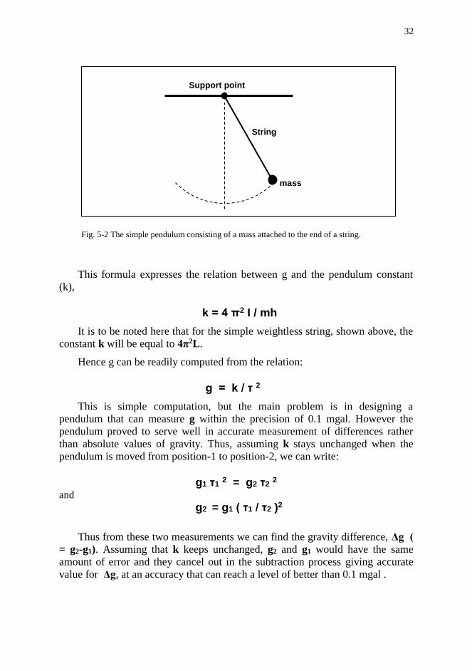
5.2.2 Swinging Pendulum
A pendulum is defined as an instrument consisting of a freely-swinging
mass which is suspended from a fixed point (Fig. 5-2). The pendulum swinging
period (τ) is the function of the pendulum constants and the earth gravity (g). For
the well-known simple pendulum, swinging with small amplitude, the period (T)
is given by the function:
τ = 2 π √ L / g
where L is the length of the string (considered to be weightless) which
connects a point mass to a suspension point. In general, τ is given by:
τ = 2 π √ I / mgh
τ2 = k / g ,
Where I is the moment of inertia about the suspension point, and h is the
distance from the suspension point to the center of pendulum mass (m).
Fig. 5-1 Sketch layout of the falling-prism instrument for measuring gravity
Falling prism
Beam splitter
Lens
Stationary
prism Laser
source
Detecting and
counting
system
32
This formula expresses the relation between g and the pendulum constant
(k),
k = 4 π2 I / mh
It is to be noted here that for the simple weightless string, shown above, the
constant k will be equal to 4π2L.
Hence g can be readily computed from the relation:
g = k / τ 2
This is simple computation, but the main problem is in designing a
pendulum that can measure g within the precision of 0.1 mgal. However the
pendulum proved to serve well in accurate measurement of differences rather
than absolute values of gravity. Thus, assuming k stays unchanged when the
pendulum is moved from position-1 to position-2, we can write:
g1 τ1 2 = g2 τ2 2
and
g2 = g1 ( τ1 / τ2 )2
Thus from these two measurements we can find the gravity difference, Δg (
= g2-g1). Assuming that k keeps unchanged, g2 and g1 would have the same
amount of error and they cancel out in the subtraction process giving accurate
value for Δg, at an accuracy that can reach a level of better than 0.1 mgal .
mass
String
Support point
Fig. 5-2 The simple pendulum consisting of a mass attached to the end of a string.

33 Chapter 5 : Gravity measurements
A standard portable pendulum, the Gulf Pendulum (Fig. 5-3), was used in
geophysical exploration during the 1930s. It consists of glass bar with wedge-
shaped supports on either side resting on glass plates which were attached to a
heavy frame. The swinging mass is attached to a wedge which is resting on a
stationary platform. The pendulum is encased in a vacuum chamber which is
thermostatically controlled to maintain stable temperature.
The Gulf Pendulum was used by G. P. Woolard (1908-1978) and his group
in establishing the world-wide network of gravity base-stations during the years
around 1960.
5.2.3 Spring Gravimeter
Unlike the falling weight and pendulum instruments gravimeters are
designed to measure gravity differences rather than absolute gravity values. In
principle, a gravimeter is a refined version of the spring balance. The extension
of the spring depends on the pulling force. As it is shown in Fig. 5-4, the
gravitational force (mg) is balanced by the spring upward force (kx). That is:
mg = kx
Fig. 5-3 Sketch showing the structure of the Gulf pendulum.
Fixed platform
Moving mass
Wedge

34
This means that any change in gravity (Δg) produces a corresponding
change (Δx) in the spring length. Since:
m Δ g = k Δ x
and
Δx/ Δg = m/k
It should be noted here that the spring balance differs from the beam balance
in that it determines weight (force) and not mass. That is why the spring balance
is used for gravity changes whereas beam balance is unable to detect such
changes.
In a gravimeter, a mass is attached at the end of a spring and when gravity
increases the spring is stretched by a proportional amount. Thus from direct
measurement of the change in the spring length (Δx) the gravity change (Δg) is
determined from Δg = k Δx/m.
A gravimeter is required to detect gravity changes of 0.1 mgal (one in ten
millions of the earth gravity). The spring of a gravimeter is about 30 cm-long,
which means that it is required to measure length change in the order of 0.03
microns (3x10⁻⁶ cm). For this reason, gravimeters employ magnification
processes based on either optical, electrical or mechanical techniques.
Fig. 5-4 Principles of the spring balance
x
Δx
kx
mg
k(x+Δx)
m(g+Δg)
m
m

35 Chapter 5 : Gravity measurements
It is worth noting that this type of a spring system (similar to a seismometer)
has a natural period (τ), when it is freely vibrating in vertical direction. τ is given
by:
τ = 2 π √ m/k Using the equation (Δx / Δg = m/k ), we get:
Δ x/ Δ g = (τ / 2 π)2
This means that, the system sensitivity (Δx/Δg), which is proportional to τ2,
can be increased by choosing the system-parameters in such a way as to get
larger natural period (τ). That is getting greater change in the spring length for a
given gravity change.
All gravimeters are sensitive to changes in temperature, pressure and to
earth seismic tremors, and all these effects are taken into consideration in the
construction-design.
According to their construction-designs, gravimeters are divided into stable
and unstable types:
5.2.3.1 The Stable Type of Gravimeters
A case of stable equilibrium is represented by a body that tends to return to
its rest position if it were slightly displaced. The unstable equilibrium case, on
the other hand, is the case where the body tends to move farther away from its
original rest position.
In the stable type of gravimeters, the spring used is of stiffness (k) which is
as low as possible to give highest possible sensitivity while at the same time it is
strong enough that can support the suspended mass (m). Examples of stable
gravimeters are Hartley and Gulf gravimeters.
The Hartley gravimeter is one of the simplest examples of the stable type of
gravimeters. The vertical motion of the mass is magnified about 50,000 times by
a system of mechanical and optical levers. It is the first gravity instrument that
used the principle of the null method by which the displacement is measured
through adjustment of an auxiliary spring (Fig. 5-5).

36
The accuracy of this gravimeter is only about one milligal which is not
sufficient for normal gravity exploration work.
The Gulf gravimeter consists of a mass attached to the lower end of a
helical spring which is made in the form of a helix with the flat surfaces always
parallel to the spring axis (Fig. 5-6).
When the gravity increases the spring is rotating as well as increasing in
length. In the Gulf gravimeter, the rotation is magnified by a system of mirrors
giving an accuracy of 0.02 mgal.
Fig. 5-5 Schematic representation of the Hartley gravimeter
Mass
Micrometer screw Eyepiece
Light beam
Mirror Beam
Hinge
Light source
mg
Ad
jus
tin
g s
pri
ng
Ma
in s
pri
ng

37 Chapter 5 : Gravity measurements
5.2.3.2 Unstable type of Gravimeters
In the design of this type of gravimeters, extra sensitivity is gained by
making the system unstable about the null position. A principle, called
astatization or labilization, is introduced to achieve this objective. In an astatized
system the gravitational force is kept in an unstable equilibrium with the
restoring (stabilizing) force. The instability feature is provided by an extra force
which acts in the same direction as the gravitational force and in opposition to
the restoring force. This extra force, called astatizing or labilizing force, is
created once the suspended gravimeter mass is shifted from the null
(equilibrium) position. The astatizing force acts as an agent that intensifies the
effect of the gravity change with respect to the equilibrium value. This feature
would greatly increase the measurement-sensitivity of the instrument.
One example of this unstable type of gravimeters is Thyssen gravimeter. As
illustrated in Fig 5-7, the astatizing force is provided by an auxiliary mass (m).
The main mass (M) which is suspended from one end of the gravimeter beam is
balanced against the spring stabilizing force (kx).
The auxiliary weight is put exactly above the pivot which is balanced in an
unstable equilibrium. A small change in g will cause the beam to tilt and the
mass
Fig. 5-6 Schematic representation of the Gulf gravimeter.
Heli
ca
l s
pri
ng
mg

38
auxiliary mass to move in the same direction, bringing about an additional
couple which reinforces that of the changed gravitational force. This causes an
additional increase in the spring length which is proportional to the change of
gravity. The precision of an observation achieved with this gravimeter is about
0.25 mgal.
LaCoste-Romberg Gravimeters
It consists of a hinged beam carrying a mass (M) which is supported by a
spring. As shown in Fig 5-8, the angle between the spring and the beam (θ1)
changes with the change in gravity (Δg). This change will cause the moment of
the spring on the beam to vary in the same sense as that of the moment created
by the gravitational change. This kind of design would provide the required
instability equilibrium (i.e. astatization effect) which magnifies the effect of
gravity change. Measurement of the changes is made by applying the null-
principle where an adjusting screw is turned to change the support position of the
main spring.
Fig. 5-7 Schematic representation of the Thyssen gravimeter.
Auxiliary
mass, m
Light
beam
mirror
Scale
Astatizing
force
Beam tilted at
g = g0 + Δg
M (g0 + Δg) Mg0
Main
mass, M Spring
Pivot
Beam horizontal at
g = g0

39 Chapter 5 : Gravity measurements
Fig. 5-8 Schematic representation of the LaCoste-Romberg gravimeter.
Adjusting
screw
Main spring
Beam
Hinge M(g0+Δg)
θ1
θ2
Mg0
Through electrical heating coils (thermostat device), the temperature of the
system is maintained within 0.002 C and its measurement accuracy can be up to
0.01 mgal.
The LaCoste-Romberg gravimeter has an additional feature which is the use
of the so called “zero length” spring. In the zero position of the gravimeter beam,
the main restoring spring is designed in such a way that the beam weight is
counteracted by an extra tension put into the spring when it is manufactured.
This means that the beam, in its null position, produces zero extension in the
spring. This kind of spring (called “zero length” spring) can be made by twisting
and coiling a wire at the same time. Effectively the extension of the zero-length
spring from equilibrium state caused by the beam weight in its null position is
counteracted by the extra tension put into the spring when manufactured.
The advantage of the zero-length spring is that the beam deflection will be
symmetrical about the equilibrium position. That is a positive reading and
negative reading for the same magnitude of gravity change will be equal.
Another advantage gained from the use of such springs is that the spring can be
shorter than normal length for the same amount of sensitivity (Dobrin, 1960).

40
There are different models of LaCoste-Romberg gravimeters. Fig. (5-9)
show two models (G and EG) of Romberg gravimeters.
Fig. 5-9 Show two models of LaCoste-Romberg gravimeters. Aliod G gravimeter (left side)
and EG gravimeter (right side).
The modification changes of LaCoste and Rumberg gravimeters leads the
mode of acquisition to a digital read-out and/or logging of the gravity
measurement and no longer necessity to read through the eye-piece, the accuracy
and repeatability of the instrument are much less subjective. Another
modification changes the battery pack to a lithium-ion rechargeable that is
located on the meter itself. The Gravition EG model specification are self-
leveling, all meter functions are fully automated, most sensitive, data resolution
24-bit less than 0.0001 mgal bit size. In addition it is provide with a
monochrome VGA LCD with backlight digital display, 32MB Flash RAM
Memory (up to 100,000 stations) and integrated data logger.
Worden Gravimeter
The Worden gravimeter (introduced in 1948) consists of a small beam
supported by a zero-length spring (Fig 5-9). The pointer is viewed through an
eyepiece to see that it is back to the null position when the micrometer screw is
turned. Differences in dial readings are converted into gravity units by use of the
scaling factor of the instrument. Thermal compensation is affected by the
differential expansion system which compensates temperature effect on the
spring.

41 Chapter 5 : Gravity measurements
The design of the instrument is similar to that of the Lacoste-Romberg
gravimeter. It is smaller (about 35cm high, 18cm in diameter and of weight less
than 4kg and it has the capability of measuring large gravity change reaching
more than 5200 mgal. Its accuracy reaches 0.01 mgal (Dobrin, 1960),
The Worden gravimeter became popular for its convenient size, weight and
easy manipulation. It has a temperature compensation mechanism and of highly
efficient thermal insulation. The instrument is entirely non-magnetic. It is read
by the null-method and requires no clamping.
Scintrex gravimeter
It consists of a mass-and-spring assembly put in a vacuum chamber.
Movement and null adjustment are made through electric transducer. The direct-
current, feed-back voltage is proportional to gravity changes which are stored in
the provided computer memory. Accuracy attained by this gravimeter is about
0.01 mgal (Robinson, 1988).
CG-5 Autograv Gravimeter
The new CG-5 Autograv system from Scintrex is one of the most versatile
and advanced gravity systems for mineral exploration, oil and gas exploration
and microgravity applications. The Autograv is a microprocessor-based
automated gravity meter that has a measurement range of over 8000 mGals
Fig 5-10 Schematic representation of the Worden gravimeter.
Po
inte
r
Ze
ro-l
en
gth
ma
in s
pri
ng
m
mg0
Ad
jus
tin
g s
pri
ng
Weight arm
m (g0 + Δg)
Hinge

42
without resetting and a reading resolution of 0.001 mGal. This enables the
Autograv to be used for both detailed field investigations and large scale
regional or geodetic surveys.
Accurate measurements are taken by
simply pressing a key and under most
conditions it takes under one minute to
complete the reading. A series of readings
of gravity measurements can be performed
by setting the Autograv in the auto-repeat
mode.
The individual readings are displayed
directly in mGals. The data is stored in
Flash memory and can be sent to a printer,
modem, recorder or PC. The station
positions are measured with the integrated
GPS capability; the internal GPS and
precise clock for X-Y positions and earth
tide corrections and external GPS input for
Z-position and altitude corrections and
real time free air and Bouguer corrections. Fig. 5-11 CG-5 Autograv gravimeter
The LaCoste-Romberg and the Worden gravimeters are examples of
unstable gravimeters that use zero-length springs.
Vibrating-String gravimeter
This type of gravimeters (Robinson,1988) uses the concept of dependence of
vibration-frequency (f) of a fiber string supporting a suspended mass (M) on
gravity (g). The relation is expressed by the following formula:
f = [Mg / 4x2m]1/2
Where m is the mass per unit length of the string and x is the string length.
Gravity changes are measured electronically. This type of gravimeters is still in
the research state and they may become the future surveying-gravimeter.

43 Chapter 5 : Gravity measurements
5.3. Instrument Calibration
Observations with a gravimeter are recorded in arbitrary scale
divisions. To convert these divisions to milligals, it is necessary to calibrate the
instrument that is to find a scale-division-to-milligal conversion factor. One
method is to measure gravity at two points where the gravity difference between
them is known, such as two base stations or top and bottom of a building with
allowance for the building contribution. Another method is the use of a tilt table.
In this method, gravity component (g cosθ) is varied by varying the table tilt,
where θ is the angle of tilt.
To illustrate the method assume that two readings were taken at the two
points A and B where the gravity at each of them is accurately known. For
example, let the readings be 120.53 mgal corresponding to 359.60 s.d. at station
(A) and 57.30 mgal corresponding to 233.14 s.d. at station (B). By dividing the
difference 63.23 mgal by the difference 126.46 s.d. we get the conversion factor
0.50 mgal per scale division.
5.4. Instrumental Drift
Gravimeters normally exhibit time-variant changes in their dial reading.
The continual variation in the instrument reading observed over a defined time
interval is caused mainly by the slow and continual creep of the gravimeter
springs as they are not perfectly elastic bodies. The phenomenon of time-variant
changes in the gravimeter reading, which are caused by mechanical and
temperature effects, is known as instrumental drift.
It so happened that a gravimeter reading is simultaneously affected by
another time-variant gravity changes. This is the tidal effect due to the sun and
moon gravitational attraction. The tidal effects make the measured gravity
fluctuate slightly with time introducing its own gravity component superimposed
upon the other instrumental-drift component. The combined time variant-
changes over a certain time interval are normally displayed in the form of a
graph. The separation of the two effects is facilitated by the fact that the tidal
component changes in a cyclic manner. The drift, on the other hand, changes
fairly linearly especially when the observation is made over short time-intervals
(Fig 5-10). The total tidal- and drift-effects is in the order of a fraction of a
milligal. An alternative way to separate the tidal fluctuation component is by use
of a special equation depending on sun and moon positions in relation to the
observation point.
In a field gravity survey the instrumental drift is determined for each point in
the survey area and corrected for accordingly.

44
The instrumental drift can be determined only by repeated observations at
the same site. Gravimeter drift may be of uniform variation where it is estimated
to be in the order of about less than one milligal per week, or irregular and high,
reaching one milligal per day. In normal surveying, a base station is reoccupied
at least once every three hours during a work session. This is a necessary
procedure for the establishment of a representative drift-characteristic curve for
the employed gravimeter.
Fig. 5-10 Example of a drift curve
9 10 11 12 01 02 03 04 05 06 07 08 09 10
AM Time of day PM
Mil
lig
al
0
+0.1
+0.2
-0.1
-0.2
-0.3

Chapter 6
GRAVITY FIELD SURVEYING
6.1. Land Gravity Surveying
Gravity surveying involves measuring the gravity values at defined locations
(the survey station-points or stations) which are distributed throughout the
assigned survey area. In addition, other measurements and pertinent data must be
made available. These are the supporting data which principally include location
coordinates (latitudes and elevations) and times of the readings. These data are
necessary for computing the gravity anomaly in a later processing stage.
6.1.1 The Gravity Field Data
The Earth gravitational acceleration (i.e. the gravity, g), measured at any
point on the Earth surface, is the vector sum of a number of gravity components.
The gravimeter reading changes with position (xyz coordinates), and with time
(t) to some extent. These changes, as it is explained in the chapters 3 and 4, are
due to a group of factors which are of global and local origins.
In gravity field surveying, the gravity values are measured over a defined
grid of points distributed over the survey area. The gathered gravimeter readings
at the grid points (observation stations) form the basic raw data from which the
gravity component caused by the subsurface geological anomaly is then isolated.
As it is with the case of seismic field surveying, gravity field data may be
divided into two types. These are:
The gravity values furnished by the gravimeter measurements (the gravity
readings).
The supporting data which cover all other data necessary for data reduction.
Most important of these are position and time coordinates (xyz and t) in addition
to the full picture of the surface terrain of the survey area.
A land gravity survey is normally conducted through two operation phases.
These are: establishment of the base-station network and documenting the
gravity readings at all of the station-points in the survey area. A location map
with an adequate scale must be first made available (Fig. 6-1).
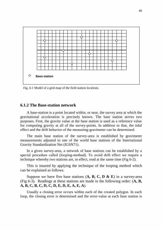
46
6.1.2 The Base-station network
A base-station is a point located within, or near, the survey area at which the
gravitational acceleration is precisely known. The base station serves two
purposes. First, the gravity value at the base station is used as a reference value
for computing gravity at all of the survey-points. In addition to that, the tidal
effect and the drift behavior of the measuring-gravimeter can be determined.
The main base station of the survey-area is established by gravimeter
measurements adjusted to one of the world base stations of the International
Gravity Standardization Net (IGSN71).
In a given survey-area, a network of base stations can be established by a
special procedure called (looping-method). To avoid drift effect we require a
technique whereby two stations are, in effect, read at the same time (Fig 6-2).
This is insured by applying the technique of the looping method which
can be explained as follows.
Suppose we have five base stations (A, B, C, D & E) in a survey-area
(Fig 6-3). Readings at these stations are made in the following order: (A, B,
A, B, C, B, C, D, C, D, E, D, E, A, E, A).
Usually a closing error occurs within each of the created polygon. In each
loop, the closing error is determined and the error-value at each base station is
Fig. 6-1 Model of a grid-map of the field station locations
Base-station

47 Chapter 6 : Gravity field surveying
re-adjusted by distributing the closing error over the observed gravity values.
The mathematical procedure is explained in chapter 9.
In a normal working day, a base station is reoccupied at least once every
about three hours. Base station reoccupation is the way to determine gravimeter
drift characteristics which shall be later used in the data reduction stage (Fig. 6-
4).
06 07 08 09 10 11 12 13 14 15 16 17 18 19 20 21 22
Gra
vit
y i
n m
illi
ga
ls
A1
A2
B2 B1
C2 C1
D1
D2
Fig. 6-2 Base station re-occupation technique for determining the short term tide-drift curves
which are used to establish the base-station network.
Fig. 6-3 Looping-method applied in the process of establishing a base-network made-up
of five base stations ( A, B, C, D, & E )
A
B C
D
E
C E D A A B

48
It is a good practice to determine the gravimeter drift characteristics before
the start of the survey. This is done by reading the gravimeter at a certain site
once, or few times, a day for several days. However, base-station reoccupation
procedure must always be followed during the normal daily survey work.
6.1.3 The Survey Gravity Readings
The most important pre-requisite in any gravity survey project is an
adequate location map. The survey design parameters (station locations and
spacing) depend on the survey objectives. Station spacing depends on whether
the survey is reconnaissance or detailed and whether it is regional or local.
Station locations are normally defined by the corner-points of a square grid in a
uniform grid map. The length of the side of the grid-cell is function of the size of
the anticipated geological anomaly. In oil exploration it is in the order of 0.5-1.0
km, while in mineral exploration, the side-length is in the range of 10-50 m. This
becomes in the order of 1-5 m. in microgravity surveys where the objective is to
locate small-scale features such as subsurface cavities, buried archaeological
objects or relatively shallow structures of engineering interests. Survey stations
may be irregularly spaced when a sufficient number of points, of known
coordinates, are available in the area.
The daily work is started by taking a reading at the nearest local base station.
This is followed by reading the rest of the survey stations. The process is
continued with reading of the base station at regular intervals of about 2-3 hours
throughout the working day. Each day is started by reading the base station and
concluded by reading that base station at the end of the day.
Gra
vit
y i
n m
illi
ga
ls
B
B
Survey station-point readings
Time of day (hours)
Base-station
reading Base-station
reading
Drift value
Fig. 6-4 Base station re-occupation during normal survey work

49 Chapter 6 : Gravity field surveying
The gravity reading and the time at which it is taken are systematically
tabulated in the field notebook. The xyz-coordinates are also noted alongside the
gravity and time readings. An example of a field data-sheet is shown in Fig. 6-5.
Station number
Longitude Latitude Elevation Time
hours & minutes
Gravimeter reading
Remarks
Base-stn.
Stn-1
Stn-2
Stn-3
Stn-4
Stn-5
Base-stn.
Stn-6
Stn-7
…….
Fig. 6-5 An example of a field data-sheet for documenting gravimeter readings and other
supporting data.
6.1.4 Station Locations and Elevations
Station locations and elevations may be determined from the location map
which is showing the elevation as numeric data or as contour topographic map.
Modern electronic satellite navigation systems can be applied for this purpose.
To get an accuracy of 0.1 mgal in relative-gravity measurements, elevation
difference from the datum level must be of an accuracy of within 30 cm. This is
deduced from the fact that the gravity change is 0.3 mgal per meter change in
height.
There are three basic ways to determine elevation. These are: the
conventional optical (rod and telescope) method, the use of the aneroid altimeter
and the use of topographic location maps.
6.2. Marine Gravity Surveying
There are two ways to conduct a gravity survey at water-covered areas.
These are done by using gravimeters placed at sea floor or on board of a ship.
The sea-floor measurement is done using gravimeters sealed in special water-
tight containers and operated by remote control systems. The on-board method,
which is less accurate and faster to operate, suffers from problems caused by the
ship movements.

50
6.2.1 Sea-Floor Measurements
This type of surveying is commonly conducted by use of the Lacoste-
Romberg gravimeter, kept in a water-tight container. It is lowered into sea from
a ship and operated through electric cables by remote-control system. This
includes instrument leveling, clamping and unclamping of the instrument.
Most of sea-floor gravity surveying is conducted on continental shelves
where water-depth is about 200 meters. The main difficulty this method faces is
the effect of sea-waves, which can cause disturbance to the instrument especially
in shallow water areas. In such environments measurement accuracy of about 0.2
mgal can be achieved in 10-15 minutes. The water depth of the observation point
is measured by an echo-sounder.
6.2.2 Shipboard Measurements
The shipboard gravity measurements are done by gravimeters with special
mountings that can provide the necessary protection for the gravimeter from
being disturbed by the ship rolling and pitching.
As the boat moves along a survey-traverse, the on-board gravimeter system
is made to output a continuous gravity record. This is achieved by an automatic
beam-adjusting system which detects any movement of the gravimeter beam,
and activates a mechanical device that restores the beam position. The gravity
value is recorded from measuring the electric current required for the beam
restoration.
Although it is relatively faster in covering a marine gravity survey, this
method suffers from some problems introduced as a result of the non-static
nature of the survey-ship. The on-board gravimeter responds to the resultant of
all of the gravitational changes including those created by the motion of the ship.
These are generated from three main sources:
- Pitch and roll of the ship that can tilt the gravimeter.
- Vertical motion (rise and fall) of the ship.
- Ship travel-motion over the curved sea-surface path.
To overcome the pitch and roll effects, the gravimeter platform is kept in
horizontal-level by free-swinging gimbals with additional gyroscopic
stabilization system.
The imposed vertical-acceleration effect is treated in two ways. First, the
gravimeter beam is designed in such a way as to be with a long-enough natural

51 Chapter 6 : Gravity field surveying
period (longer than sea-wave period) and by a damping device fitted to the
gravimeter-beam (Fig. 6-6).
For the third type of effects, the acceleration contribution from the ship
travel motion is function of the ship travel-velocity (speed and direction). This is
corrected for in the processing stage. The gravity correction which compensates
for ship-movement is called Eotvos Correction, after Baron Von Eotvos (1848-
1919).
6.2.3 Eotvos Correction
Marine gravity measurement made by a gravimeter on board of a moving a
ship is influenced by additional forces created as a result of the ship motion
during the measuring process. Unlike land surveying, where the gravimeter is
stationary during the measuring process, a shipboard gravimeter is moving with
a certain cruising velocity (speed and direction) while it is measuring. In its
motion, the ship (Fig. 6-7) moves over the sea surface along a curved path which
forms a segment of a great circle of the Earth. Thus a gravimeter on board of a
cruising ship would experience a centrifugal force (acceleration) due to its
motion over a circular path. In addition to that, there is another factor that
influences the gravimeter reading and that is the effect of the ship velocity on the
centrifugal force (centrifugal acceleration) created by the Earth rotation about the
Spring
Hinge Beam
Damping
system
mass
Fig. 6-6 Principle of beam-damping system fitted to shipboard gravimeter.

52
polar axis. As a result, the gravimeter will be measuring different values of
gravity from that detected by a stationary gravimeter located at the observation
point. The correction which is made to remove the effects due to ship motion
from the shipboard-gravimeter reading is known as Eotvos correction.
In case where the measuring instrument is moving with a certain velocity
while it is in the measuring process, it experiences centrifugal force due to this
motion. This will incur a change on the gravity value if it were measured while it
is at rest.
An eastward component of the ship velocity would add-up to the Earth
rotation-velocity causing increase of the centrifugal acceleration which in turn
causes the gravity reading to decrease. An opposite effect results from a
westward velocity-component. The gravity reading must therefore be corrected
for this effect. The correction is called Eotvos correction.
The Eotvos correction (EC) in milligals, due to the velocity of the ship
carrying the gravimeter, is given by Telford, et al ,(1996):
EC = 4.040 V cosΦ sin α + 0.001211 V2
Fig. 6-7 Generation of an additional centrifugal acceleration due to the motion
of the gravimeter-carrying ship over a segment of a great circle and at the same
time rotating about the Earth polar axis .
V
VN
VE
East
North
α
ø
Ship
Great
circle

53 Chapter 6 : Gravity field surveying
Where V in km/hour is the ship velocity, Φ is the latitude of the
measurement location, and α in degrees, represents the ship-path bearing which
is measured from the geographical North.
The value of EC is positive (to be added to the measured gravity-value)
when the ship is moving in westerly direction, i.e. when its velocity (V) has an
East to West component, and it is negative when the ship is moving in easterly
direction. The finally corrected value will be the value of gravity corresponding
to that obtained for a stationary observation point at that location.
In summary, marine surveying may be carried out through measurements of
gravity on sea floor or on sea surface. Each of these two methods has its own
merits and problems. The sea-floor method needs gravimeters enclosed in water-
tight casing and fitted with remote-control systems for their operation. This
method is of high sensitivity but it is slow because of the lengthy transportation
of the gravimeter between observation stations.
The other shipboard method is the more widely used technique where the
gravimeter is mounted on board of a moving ship. In this case, a specially
stabilizing instrument-base, must be provided to lessen the effect of ship due to
rolling and pitching movements caused by the sea waves. Another and more
important feature of this method is the gravity effect caused by the ship velocity
of travel. Thus an eastward velocity-component would add-up to the Earth
rotation-velocity causing increase of the centrifugal acceleration which in turn
causes the gravity reading to decrease. An opposite effect results from a
westward velocity-component. The measured gravity in this case must be
subjected to correction called Eotvos correction.
6.3. Airborne Gravity Surveying
As in the seaborne gravity surveying, airborne surveying suffers from the
non-static nature of the measuring instrument. Error values in the airborne
measurements are larger than those found in seaborne surveying due to more
rapid change in aircraft altitude and other types of motion.
Experimentation with the use of helicopter began 1971. Reduced flight-
speed in this case leads to improvements in the accuracy of both of Eotvos
correction and navigation data. In calm weather and careful navigation, the
accuracy in the range of few milligals can be obtained.
There are further two types of effects resulting from airborne gravity
measurements. These are the aircraft height above land surface and the terrain
gravity effects. Both of these factors lead to diminishing of the detected gravity

54
anomalies. Due to these problems, helicopter gravity surveying is used for
reconnaissance surveying where the accuracy is in the range of few milligals. In
such practices, the gravimeter is fitted with the appropriate devices that secure
stability and reduce external acceleration changes.
6.4. Microgravity Surveying
On the basis of the size of the objective exploration targets, a gravity
surveying may be rated as large-, medium-, or small-scale survey projects.
Large-scale gravity surveying projects aim at exploring features such as shape of
the Earth, crustal-thickness variation, and isostatic compensation. The medium-
scale surveying, on the other hand, includes studying geological structures such
as igneous intrusions, sedimentary basins, hydrocarbon traps, and ore bodies.
In the later years, gravity surveys were designed to detect and delineate
small scale structures of the type which serve engineering and archaeological
purposes. In particular, fracture zones, subsurface cavities and buried ancient
relics. Gravity surveying designed for this type of purpose is commonly referred
to as microgravity surveying. The type of gravimeter used in microgravity
surveys is one which is capable of detecting gravity changes as small as one
microgal (= 0.001 milligal).
The main features of a microgravity survey are the closely-spaced
observation points (1-5 meter) and the high measurement precision in detecting
gravity anomalies which are in the order of 0.001-0.002 milligal.
Interpretation of microgravimetric data is based on relative gravity
measurements and thus no need to have absolute gravity values for the
interpretation process.
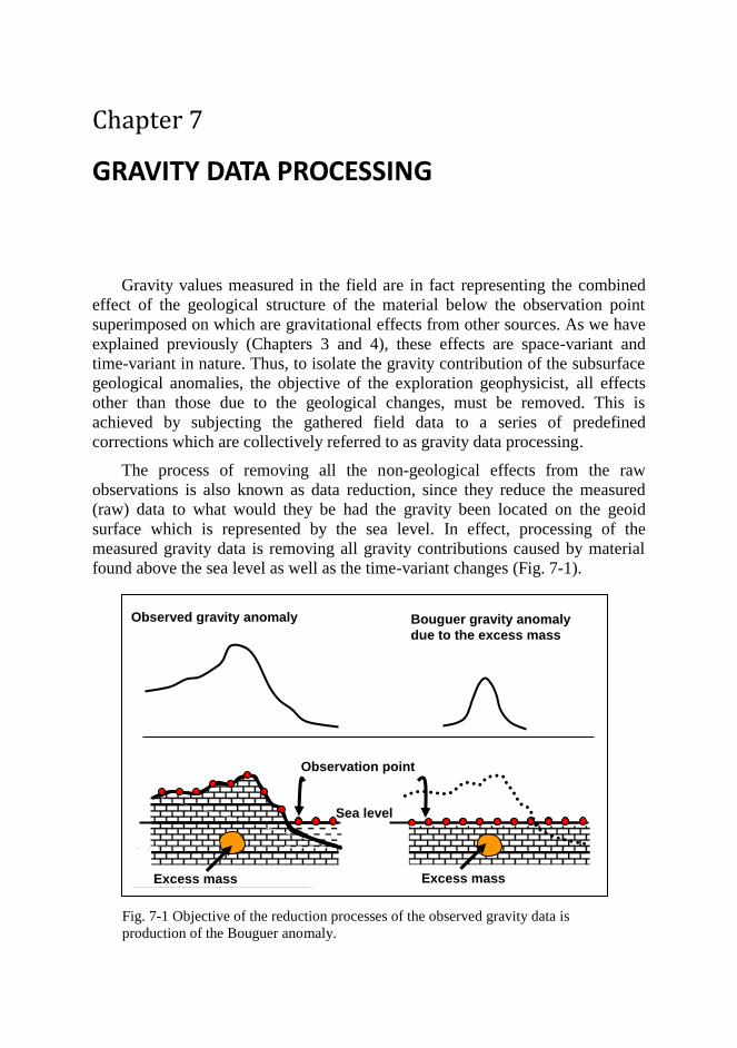
Chapter 7
GRAVITY DATA PROCESSING
Gravity values measured in the field are in fact representing the combined
effect of the geological structure of the material below the observation point
superimposed on which are gravitational effects from other sources. As we have
explained previously (Chapters 3 and 4), these effects are space-variant and
time-variant in nature. Thus, to isolate the gravity contribution of the subsurface
geological anomalies, the objective of the exploration geophysicist, all effects
other than those due to the geological changes, must be removed. This is
achieved by subjecting the gathered field data to a series of predefined
corrections which are collectively referred to as gravity data processing.
The process of removing all the non-geological effects from the raw
observations is also known as data reduction, since they reduce the measured
(raw) data to what would they be had the gravity been located on the geoid
surface which is represented by the sea level. In effect, processing of the
measured gravity data is removing all gravity contributions caused by material
found above the sea level as well as the time-variant changes (Fig. 7-1).
Fig. 7-1 Objective of the reduction processes of the observed gravity data is
production of the Bouguer anomaly.
Bouguer gravity anomaly
due to the excess mass
Observed gravity anomaly
Observation point
Sea level
Excess mass Excess mass

56
The processing steps which are normally carried out in processing of gravity
raw data are as follows:
7.1. Instrument Calibration and Drift Correction
Gravimeter measurements are usually quoted by the instrument scale-
divisions (sd.). Thus, the instrument reading must be converted into gravity units
which are usually the milligal units. This is done by multiplication of the reading
(in sd. units) by the instrument calibration factor which is normally determined
at the start of the survey. The calibration factor is expressed in (milligal/sd)
units.
During fieldwork the instrument is read at a certain base station regularly at
2 to 3 hour intervals. The gravimeter reading is plotted against time to obtain the
instrumental drift characteristics curve. From this curve, the instrument reading
can be determined at any time (between two consecutive points) by
interpolation, assuming that drift change is linear. As we have already explained
(Chapters 5 and 6), time-variant gravity changes include both of the instrumental
and tidal effects and their combined effect is expressed by the so-constructed
drift curve (Fig. 6-10).
Having constructed the drift curve, the gravimeter reading made at each
gravity station of the survey area is corrected for the instrumental-drift of the
gravimeter used in the survey.
7.2. Latitude Correction
There are two global related factors that cause the earth gravity to change
with latitude. These are the Earth flattening and its rotation about its polar axis.
This has led the Earth gravity to increase as the observation point moves from
the equator towards either of the two poles. For this reason, the Earth gravity,
measured at sea level, increases uniformly with the increase of latitude (Fig.
7.2).
Normally, the GRS67 formula in which gN(Φ) (shown in Fig 3-7) would
give the value of gravity (gN) at sea level at any point having latitude (Φ) over
the Earth surface. The value gN(Φ) is considered to be the universal reference
datum relative to which the final gravity anomaly is computed.
Latitude correction is achieved by subtracting the normal gravity (gN), from
the observed gravity value (g0) to obtain (Δg0) which is called the observed
gravity anomaly. Thus:

57 Chapter 7 : Gravity data processing
Δg0 = g0 - gN
It is important to note that if the gravity project contains mixed data in
which a data-set was corrected using the 1930-Formula and another set corrected
by GRS67 formula, unification of correction processes must be done. This is
performed using the following correction formula (Kearey and Brooks, 1987,
P151):
gN(1967) - gN(1930) = 13.6 sin2 Φ - 17.2 mgal.
7.2.1 Rate of Change of Normal Gravity
The gN value at any observation point of latitude (Φ), can be obtained from
the tables which are prepared from the GRS67 formula, or alternatively by
computing the value based on another known value (reference point), using the
formula for the rate of change of the normal gravity.
The rate of increase of the normal gravity with latitude ∆gN/∆Φ can be
obtained from differentiating the gN(Φ) equation. Within the accuracy of the
gravimeter measurements we can neglect the terms in sin4 Φ, as this will not
affect the result too much, to give:
Fig. 7-2 The Earth latitudes and longitudes serve as location
coordinates for station points in gravity surveying.
90
80
70
60
50
40
30
20
10
0 0 10 20 30 40 50
50 degrees East
60 d
eg
rees N
orth
Longitude
La
titu
de

58
∆gN / ∆Φ = 978.0327 * 0.005279 sin2Φ gal/radian
or, ∆gN / ∆Φ = 5163 sin2Φ mgal/radian or, ∆gN / ∆Φ = 90.11 sin2Φ mgal/degree
As these formulae indicate, the rate of change varies with the latitude. At
latitude of 45 degrees, the rate of change reaches its maximum value of 90.11
mgal/degree, and it is zero at the poles and at the equator (Fig. 7-3).
Since gN decreases in the direction of the equator, the gravity difference
between the observation point and the reference point must be added to that of
the observation value if the observation point is located at a latitude nearer to the
equator than that of the reference point.
Taking the Earth mean radius to be 6367.5 km which is the mean of the
equatorial radius (6378.160 km) and the polar radius (6356.775 km), the Earth
circumference becomes 40008 km and the distance corresponding to one degree
becomes 111.13 km (40008/360). The rate of change can therefore be given as
Fig. 7-3 Rate of change of the normal gravity value as function of latitude.

59 Chapter 7 : Gravity data processing
h
h
Sea level
Fig. 7-4 Free-air correction (FAC)
gravity change in milligals per one meter of the distance measured in the N-S
direction. That is:
∆gN / ∆s = 0.000811 sin2Φ mgal/meter
7.3. Elevation Corrections
Change in elevation causes a corresponding change in gravity. Change in
gravity that occurs as a result of change in elevation of the observation point is
function of thickness and density of the material found between the observation
point and the datum level, which is normally taken at mean sea level.
The correction may be divided into three parts; which are the free-air,
Bouguer, and terrain corrections.
7.3.1 Free-air Correction (FAC)
This corrects for the change in gravity due to change in the height of the
observation point. According to the universal law of gravity, gravity decreases as
the distance from the Earth center increases. The change in gravity due to change
in elevation is rated by 0.3086 mgal/meter (see chapter 4). Thus to reduce the
change in gravity to sea level, a gravity value measured at elevation (h) meter
must be done by increasing the observed gravity by 0.3086h milligal (Fig 7-4).
Correction of observed gravity to what it would be at sea level is called free-air
correction, FAC.

60
After correction we obtain an anomaly value ΔgFA called free-air gravity
anomaly expressed as:
ΔgFA = ΔgO + FAC
Hence
ΔgFA = gO - gN + 0.3086h
The correction is positive for observation points above sea level and
negative for observations which are below it.
7.3.2 Bouguer Correction (BC)
The FAC accounts only for change in elevation and no account is made for
the gravity change contributed by the rock-mass found between the sea level and
the observation point. This contribution is computed on the assumption that an
infinite horizontal rock slab of thickness equal to that of the material exists
between the observation point and sea level (explained in chapter 4).
The correction (called Bouguer correction, BC) is given by:
BC = 2πGρh = 0.0419ρh mgal,
where (h) is elevation in meters and (ρ) density in gm/cc (Fig 7-5).
Fig. 7-5 Bouguer correction (BC)
Density, ρ h
Sea level

61 Chapter 7 : Gravity data processing
It is to be noted here that the combined FAC and BC correction is forming
one correction normally referred to as the combined elevation correction (CEC)
which is defined by the combined formula:
CEC = (+0.3086-0.0419ρ ) h.
The Bouguer correction for sea surface measurements (BCSS) is equivalent
to replacement of the water layer (water-depth d and density ρW) by rock layer
(density ρR) giving for sea surface observations:
BCSS = 2πG (ρR - ρW)d
The Bouguer correction (BC) must be subtracted from the observed gravity
on land, whereas it must be added to the gravity values observed over sea
surfaces since it is representing replacement of the water layer by the more dense
rock material. Bouguer correction is therefore negative on land and positive over
seas.
After applying the Bouguer correction, we obtain Bouguer gravity anomaly
(ΔgB), in milligals, which is given by the expression:
ΔgB = ΔgFA - BC
Hence ΔgB = gO - gN + 0.3086h - 0.0419ρh
In general, Bouguer gravity values are negative over most of the continental
areas and positive over oceans. In and around coastal regions, Bouguer gravity
values are near zero-level. This is a common worldwide observation.
7.3.3 Terrain Correction (TC)
The Bouguer correction is computed on the assumption that the rock
material found between the observation point and the geoid surface is in the form
of a horizontal infinite slab. Since, in actuality this is not the case, a correction is
required to allow for the irregular topography of the earth surface around the
observation point.
Elevated ground (such as hills) near an observation point creates a vertical
component in gravity attraction reducing the gravity value at that point. Holes
and valleys on the other hand represent lack of material in parts of the assumed
horizontal rock-slab. In effect, these also create vertical components which
would reduce the gravity value. Thus, in normal situations, terrain correction

62
(TC) which is always positive is introduced to compensate for the topographic
irregularities existing around the observation point (Fig. 7-6).
The final Bouguer gravity anomaly which is including the terrain correction
(TC) will take the form:
ΔgB = gO - gN + 0.3086h - 0.0419ρh + TC
The classical method used in computing terrain correction is the use of the
special chart (invented by S. Hammer in 1939) with an associated set of tables.
Hammar chart consists of a set of concentric circles which are divided by radial
lines forming compartments of varying areas.
Terrain gravity contributions of the compartments are computed based on
the following computation approach:
Consider a solid cylindrical disc of thickness (d) and radius (r), (Fig. 7-7).
The gravity attraction of a solid disc (gD) calculated at the center of its flat
surface (see chapter 9 for derivation) is given by:
GD = 2π Gρ[d + r - (d2+r2)1/2]
where r is the disc radius, d is its height and ρ is its density.
Fig. 7-6 Terrain correction (TC).
h
sea level
TC
BC
TC
vertical
components

63 Chapter 7 : Gravity data processing
Now consider a ring-disc as being formed from subtraction of a solid
cylindrical disc (radius r1, say) from a larger disc (radius r2) having a common
axis with the smaller one (Fig. 7-8).
The gravity contribution (gr) at the center of the flat surface of the ring-disc
is obtained from subtracting the gravity effect of the small cylinder (radius r1)
from that of the larger cylinder (radius r2), thus:
Fig. 7-7 Cylindrical disc used as basis for computing the terrain correction.
d r
d r2
r1
Fig. 7-8 Cylindrical ring-disc is formed from subtracting two solid cylinders
of common axis

64
gr = 2πGρ[r2-r1 + (d2+r12)1/2 - (d2+r2
2)1/2]
Now, if the ring is divided into a number (N) of equal segments (Fig 7-9),
the gravity contribution (gN) of each segment (compartment) is given by:
gN = gr / N
Hammer tables (1939) give terrain correction values computed on the basis
of circular flat-topped cylinders made up of material of density (ρ) equal to 2.0
gm/cc (Fig. 7-10).
d
r2
r1
Fig. 7-9 Cylindrical ring-disc divided into eight equal sectors used to
derive the formula for gravity effect of a sector of a ring disc at the central
point (P).
P
r1
Fig. 7-10 Part of the Hammer chart. The complete chart consists of zones (B, C, D,
…, M) varying in radius from 2m for zone-B to 22km for zone-M (Kearey and
Brooks, 1987,pp 152-153)

65 Chapter 7 : Gravity data processing
One way to compute terrain corrections is by use of Hammer chart and
equation for gr; the one mentioned above. The computation procedure is done by
placing the center of Hammer chart over the observation point on the
topographic map of the area. The chart must be drawn at the same scale as the
topographic map. The average elevation of the topography within a segment is
estimated and the difference (call it Δh) in elevation of this average from that of
the observation point is obtained. Now the terrain correction for that segment is
found by substituting Δh for d in the expression for (gr) and dividing the result
by the number (n). The process is repeated for all other compartments in the
chart then the contributions of all compartments are summed up to give the total
terrain correction (TC) for that observation point. The density term (ρ) is
substituted by the mean density of the material covered by all the compartments
entering in the computation.
The more practical procedure than using Hammer chart and equation is by
using Hammer chart and the associated tables (Dobrin, 1960, Fig. 11.9 and Table
11.1). The chart is first printed on transparent plastic sheet at the same scale as
the topographic map of the survey area. The center of circles is placed over the
observation point and the average elevation within a compartment is estimated
from the contours seen through the chart-sheet. The difference in elevation (Δh)
between the estimated average and the station elevation is determined. With this
value the TC for that compartment can be read from the tables associated with
the chart (Fig. 7-11).
r
2
1
r
1
2
1
Fig. 7-11 The procedure followed in calculating terrain correction by use of the
Hammer chart. Average elevation of the yellow compartment is estimated from the
contours crossing it.

66
The terrain correction is slow and tedious work especially when it is done
manually as has been done in the olden days. Computer based computations, as
it is normally done nowadays, require digitization of the topographic elevation of
the survey area.
In area where the topography is nearly flat, terrain correction may not
exceed 1 mgal whereas in areas of rugged terrain containing mountains, steep
cliffs and valleys, the correction may reach appreciable levels. In certain cases
terrain corrections may be unnecessary especially when the computed values are
less than the desired accuracy of the Bouguer gravity values. Computation
decision is based on computation-tests which are conducted in certain parts of
the area to find out whether TC values are small enough to be neglected or not.
7.4. Isostatic Correction
A Bouguer anomaly value is obtained with a group of correction steps which
are in effect removing all effects of material existing above sea level and
replacing the ocean water with material of average crustal density. In doing that
we are assuming that there are no density variations below sea level except those
due to the relatively shallow geological structures which the exploration
geophysicists are looking for.
According to the isostatic theory there are, in certain parts of the Earth crust,
indications of lateral density variations on large scale-extent which would cause
corresponding changes in the Earth gravity. This is supported by the large and
negative Bouguer anomaly normally observed over continental blocks and some
mountainous areas.
Airy’s isostatic model for the Earth’s crust suggests that mountain ranges
(such as the Alps and the Rocky Mountains) have roots bulging through the
upper Mantle of the Earth. Such roots (being of lower density relative to its
surrounding) would cause the Bouguer anomaly to decrease by an amount
depending on the shape of the root and its density contrast. Thus according to the
structural model suggested for the Earth crust existing below the survey area,
gravity changes (due to these large-scale crustal features) can be determined and
the Bouguer anomaly is corrected for. In so doing, the effects of the lateral
density changes as predicted by the isostatic theory are removed (Fig. 7-12).
The isostatic anomaly (ΔgI) is thus defined to be the Bouguer anomaly (ΔgB)
added to which is the isostatic correction (IC), that is:
ΔgI = ΔgB + IC

67 Chapter 7 : Gravity data processing
Under-compensation and over-compensation of topographic features are
reflected by positive and negative isostatic anomalies respectively. A
topographic feature which is perfectly compensated is expected to give zero
isostatic anomaly (more details are found in chapter 9).
The basic correction processes usually followed in normal gravity surveying
can be summarized as shown in the following sketch (Fig. 7-12):
7.5. Data Reduction of Marine Gravity Data
There are two ways to conduct a gravity survey at sea. The more practical
and faster method is to measure gravity by a gravimeter mounted on a moving
ship. The other alternative method is to carry out the measurements by a
gravimeter resting on the sea-floor. As we have seen from the previous chapter
(Chapter 6) each of these two methods has its own advantages and
disadvantages. However in either case, the gravimeter readings must undergo
certain reduction processes in order to derive the Bouguer anomaly in a form
ready for the following interpretation work.
Fig. 7-12 Principle of isostatic correction.
Observed anomaly Bouguer anomaly Isostatic anomaly
Earth crust
Earth mantle
excess mass
Mountain
root
Earth crust
excess mass
Mountain
root
Earth mantle Earth mantle
Earth crust
excess mass

68
7.5.1 Reduction of Shipboard Gravity Data
For the case of gravity measurements made on board of a stationary ship, the
Bouguer gravity anomaly (gB) is computed in such a way as to compensate for
the sea water-body existing below the ship. To start with, no free-air elevation
correction is needed here since the measurements are located at sea level.
However, the Bouguer gravity anomaly (ΔgB) is computed according to the
following equation:
ΔgB = gO - gN + 0.0419 d (ρR - ρW)
Fig. 7-12 The processing sequence normally followed in gravity data-reduction.
gN
Δg
O
Δg
F
Δg
B
Δg
I
FA
C B
C
TC
IC
gO is gravity value in milligals observed (measured) at a gravity station location gN is normal gravity value, computed from GRS67 Formula ΔgO = gO - gN , Observed anomaly, ΔgF = gO - gN + 0.3086 h , Free-air anomaly, ΔgB = ΔgF - 0.0419 ρh + TC , Bouguer anomaly, ΔgI = ΔgB + IC , Isostatic anomaly,
FAC = 0.3086 h , Free air correction BC = - 0.0419 ρh , Bouguer correction TC = Terrain correction IC = Isostatic correction

69 Chapter 7 : Gravity data processing
Where gO and gN are respectively the measured and normal gravity in
milligals. Also ρR and ρW represent the density in gm/cc for rock and sea water
respectively, and (d ) in meters, is the sea-depth under the observation point.
This formula is derived on the basis of replacement of the sea water by rocks
of average crustal density. In practice, the values 2.67 gm/cc and 1.03 gm/cc are
used for ρR and ρW respectively.
In case gravimeter measurements are read during the ship motion, the
Eotvos correction (EC) must be introduced in the correction formula. The
correction is algebraically subtracted from the shipboard gravity measurement to
give:
ΔgB = gO - gN + 0.0419 (ρR -ρW)d - EC
Eotvos correction can result in sizeable errors in this computation due to
difficulty in controlling speed and direction of the ship movement. However, the
accuracy of Bouguer anomaly of a shipboard gravity is expected to be within one
to two milligals.
7.5.2 Reduction of Sea-Floor Gravity Data
For the sea-floor measurements, the observed gravity value (gO) is corrected
to get the corresponding Bouguer gravity anomaly (ΔgB) according to the
following equation:
ΔgB = gO - gN + 0.0419 d(ρR + ρW) - 0.3086d
Where ρW and ρR are density of water (=1.03 gm/cc) and rocks (about 2.67
gm/cc) respectively, and d in meters is the water depth at the observation site.
The quantities gB, gO and gN are all in milligals.
Derivation of this formula (Fig. 7-13) is based on computing gravity change
in moving the measurement point from the sea floor to the sea surface and
replacement of the water layer of density (ρW) by rock material of density (ρR).
7.6. Accuracy of Bouguer Gravity Data
The end product of the field gravity-measurement subjected to a set of data
reduction processes, is the final Bouguer anomaly map. This map will show the
variation in gravity caused by the subsurface geological structures which are
showing lateral density variations. The amplitude of the Bouguer anomaly

70
depends not only on the value of the density contrast but also on shape and depth
of the causing geological anomaly. Bouguer gravity maps are normally displayed
in the form of gravity contours drawn with an adequate contour interval.
Bouguer anomaly maps serve as the basic data used in the interpretation
phase to explore the subsurface geological structures such as anticlines, salt
domes, ore-bodies, or even subsurface empty cavities. Being dependent on
instrument measurements in the field data acquisition stage of the survey work
and on approximations in the following processing stage, Bouguer anomaly
value is expected to bear certain amount of error. In order to evaluate the
accuracy of these data on which our interpretation reliability depends, it is
important to identify the error sources and assess the extent of their effects.
(1) Error in Instrument Reading
Modern gravimeters which are carefully drift corrected can be read with
accuracy close to 0.01 mgal. This forms a measurement sensitivity in reading
changes in the Earth gravity reaching (10-8) which is adequate for normal gravity
surveys. In practice, the gravimeter gives the readings in scale-divisions which
are converted into milligals using the instrument calibration factor expressed in
milligals per scale division.
Fig. 7-13 Bouguer correction for the case of sea-floor gravity measurements
dh
Sea surface
Water density, ρw
Sea floor Rock density, ρR
Measurement location

71 Chapter 7 : Gravity data processing
(2) Error in Location
According to the normal gravity formula (gN), the rate of change of the Earth
gravity (ΔgN) with respect to distance (s), measured in the N-S direction, is given
by:
ΔgN / Δs = 0.811 sin 2Φ mgal/km
The maximum value of the change rate is at latitude of 45°, where it attains
a value of 0.811 mgal/ km, or 0.0008 mgal/m.
From this result it can be concluded that an error in location of an
observation point of one meter may introduce a corresponding error of 0.0008
milligals in the applied value of gN. Such an error becomes even smaller in
magnitude as the observation point moves towards the equator or towards the
poles. It is therefore apparent that location coordinates can tolerate a relatively
large error as far as latitude accuracy is concerned. Thus an error in location of
say 100 meter in the N-S direction would introduce less than 0.1 mgal.
(3) Error in Elevation
The equation for the elevation correction includes two parameters, the
contrast in density (ρ), and elevation (h). Thus considering ρ = 2.0 gm/cc, we
have for the combined elevation correction (CEC):
CEC = 0.3086 h - 0.0419 * 2.0*h = 0.2248 h
This formula shows that the error in elevation would cause a corresponding
error in the computed Bouguer-anomaly value of about 0.2 mgal/meter. Hence to
attain a Bouguer value to the accuracy of 0.1 mgal, elevation must be accurate to
within 50 cm.
(4) Error in Terrain Correction
The errors introduced in computing the terrain corrections come from the
rough estimation of the mean height of the topography and from the uncertainty
in the value of the rock density used for the correction. In general, this varies
from (0.05) to (0.30) mgals (Bott and Masson-Smith, 1957).

72

Chapter 8
THE GRAVITY ANOMALY
8.1. Concept of the Gravity Anomaly
As far as gravity data is concerned, a geological anomaly is defined as
any lateral change occurring in the subsurface geology of the area. This can
happen as a result of either change in density of a horizontal layer or change in
the horizontality of a constant-density layer (Fig. 8-1). In either case, such a
geological anomaly would create the corresponding disturbance in the gravity
field, known as the gravity anomaly. It is called regional gravity anomaly when
it describes large-scale geological changes and residual anomaly when the
changes are of localized nature.
Fig. 8-1 A gravity anomaly is created by a local geological anomaly with lateral changes
in depth or in density or with both.
ρ1
ρ3
ρ2
Depth lateral change Density lateral change Neither depth nor density
lateral change
Gravity anomaly No gravity anomaly Gravity anomaly
ρ
4

74
A gravity anomaly at an observation point is formally defined as the
deviation of the gravity value (corrected to the Earth ellipsoid) from the
theoretical value computed at that point. The type of anomaly depends on the
corrections made in the data reduction. The free-air anomaly is obtained if only
the free-air correction has been applied to the observed data. The Bouguer
anomaly is, on the other hand, obtained when both of free-air and Bouguer
corrections have been applied.
A Bouguer anomaly (non-zero gravity value) indicates lateral density
changes. If the density of the rock material below sea level varies only with
depth (i. e. no lateral variations), no Bouguer anomaly is created, that is the
anomaly is of zero value. Local density contrast (surplus or deficit) of the
material below sea level would give non-zero Bouguer anomaly.
8.2. Computation of Gravity Anomalies
Study of gravity anomalies associated with anomalous masses of simple
geometrical shapes is useful to gravity interpreters. Information on the
theoretical function of the gravity anomaly of certain geological models is very
useful since it gives indications on depth, shape, and density distribution of the
anomalous mass.
In the field measurements, gravimeters measure Δg which is the vertical
component of the gravitational acceleration due to an anomalous subsurface
mass. The vector quantity (Δg) is function of its depth, geometrical dimensions
and density contrast (ρ) which is the difference in specific gravity between the
material of the body and that of the surrounding medium.
Here-below, mathematical formula of the vertical component (Δg) for the
most common simple geometrical models are theoretically computed. Derivation
is based on Newton's Law of gravitation (F=G m1 m2 /r2) and Newton's second
law of motion which relates the acceleration vector (Δg) to the attracting mass of
the model.
The models dealt with here are presented under the following categories:
Spherical shapes
Cylindrical shapes
Sheets and Slabs
Rectangular parallelepipeds
Bodies of irregular shapes

75 Chapter 8 : The gravity anomaly
8.3. Spherical Shapes
8.3.1 Point Mass
The vertical component of gravity effect Δg of a point mass (Δm) buried at
depth (z) which is at distance (r) from an observation point (P) located on the
surface, is given by (Fig. 8-2):
Δg = G Δm cosθ / r2
or, since r = (x2 + z2)1/2
Δg = G Δm z / (x2 + z2)3/2
8.3.2 Spherical Shell
Consider a spherical shell (hollow sphere) of radius (R), density contrast
(ρ), and thickness (t). The gravitational attraction at a point located at distance
Fig. 8-2 The gravity anomaly due to a point-mass (A) and due to a sphere (B)
at depth z.
Z
X
(A) point-mass (B) sphere
X
Gravity
anomaly, ∆g
X
Z
X
R
r r
θ
θ
P P
0 0

76
(r) from its center is derived by considering an elementary ring (width δs = Rδθ)
cut from the sphere at right angles to the distance (r), as shown in Fig. 8-3.
Choosing the ring to be perpendicular to the line joining the observation
point (P) with the center of the spherical shell, insures that each point
(infinitesimal element) of the ring is at the same distance (s) from the point (P).
Thus, at (P), the gravity component [Δg]ring (which is acting along the distance
(r) towards the shell center) due to the elementary ring is given by:
[Δg]ring = (G. Rδθ. t. 2πRsinθ.ρ / s2 ) cosΦ
By making the substitutions:
cosθ = (R2 + r2 - s2) / 2Rr,
cosΦ = (s2 + r2 - R2) / 2sr,
sinθ dθ = s ds / Rr ,
and integrating with respect to the variable (s) from (s=r-R) to (s=R+r), we
get the gravity effect at the external point (P) for the whole shell. That is:
[Δg]sh = 4πGρtR2/r2
or
[Δg]sh = Gmsh/r2
where msh is the mass of the complete spherical shell.
s
r
Φ
θ
δθ R
P
Fig. 8-3 An elementary ring cut from a spherical shell.
Spherical shell
Elementary ring

77 Chapter 8 : The gravity anomaly
This result has shown that a spherical shell has the same gravity effect of a
point mass having the mass of the spherical shell located at its center. It can be
also shown that the gravity effect at a point located inside the shell is zero
regardless of the point-distance from the shell center. This can be proved by
carrying the integration from s=R-r to s=R+r,
8.3.3 Solid Sphere
By considering a solid (full) sphere to be consisting of infinite number of
elementary thin shells, the gravity effect of the sphere at an external point (P) at
distance (r) from its center is obtained from integrating the gravity effects of all
of the infinite number of shells considered to be making up the sphere (Fig 8-4).
Since the distance (r) is the same for all shells, the gravity effect (Δg) of the
solid sphere at (P) is obtained by multiplying the summation of the shell masses
(mass of the sphere, m) by G/r2. That is:
Δg = Gm/r2
This significant result tells that, as in the case of a spherical shell, the gravity
effect of a solid sphere, at an external point located at distance (r) from its
center, is the same as that due to a point-mass having the mass of the sphere and
located at the sphere center. In other words, the gravity effect of a sphere at an
external point (located outside the sphere) is the same as though the whole mass
of the sphere is concentrated at the sphere center.
Now, if the observation point (P) is located inside the sphere (r<R), the
gravity effect at P of a homogeneous sphere of density (ρ) will be given by:
[Δg]sphere = G (4π / 3) r3 ρ / r2
[Δg]sphere = G (4π / 3) ρr
In this case (observation point is inside the sphere) the gravity effect, which
is the vector acceleration (Δg) in the direction of the sphere center, is
proportional to distance (r) and not to (1/r2). The part of the sphere between
radius (r) and radius (R) can be considered to be made up of infinite numbers of
shells which have zero gravity effect at point (P) as shown above. This means
that Δg is of zero value at the center of a homogeneous solid sphere.

78
Gravity Anomaly of a Buried Sphere
In gravity surveying, the measuring instruments are designed to measure
only the vertical component of gravity effects of anomalous bodies that are
buried at certain depths below ground surface. Customarily, surveying is
conducted by measuring of the gravity effect over linear traverses. In other
words, the gravity variation is established as a function of horizontal distance on
the ground surface.
The gravity anomaly (vertical component of gravity, Δg) of a buried sphere
of mass (m), radius (R), and depth of its center-point (z) can be expressed as
function of distance (x) as follows (Fig. 8-5):
Δg = (G m / r2) . cosθ
Δg = 4πGρR3z / 3 (x2 + z2)3/2
and,
Δg = Δgmax ( 1 + x2 / z2 )-3/2 where,
Δgmax = Δg, at x = 0 That is, Δgmax = 4πGρR3/3z2 = 0.02794 R3ρ/z2 (R and z in meters)
Fig- 8-4 Principles of computing gravity effect of a solid sphere at a point (P) outside
or inside the sphere
Point (P) outside sphere
(r>R)
Point (P) inside sphere
(r<R)
P
r
R
P r
R

79 Chapter 8 : The gravity anomaly
As an example for application, a sphere with the radius of 500 m and density
contrast of 0.4 gm/cc having its center at 2km-depth will have a maximum value
of gravity directly above its center, [Δg]max = 0.349 mgals.
It is apparent from these formulae that [Δg]max will reduce by a factor of 1/4
when the depth of the sphere is doubled, and increase by a factor of 8 when the
radius is doubled. Another significant note is that the anomaly curve (Δg) is
symmetrical about the origin, and that the maximum amplitude of the anomaly
(Δgmax) varies inversely with the square of depth of the center. It is also
important to note that it is not possible to determine (ρ) and (R) separately from
a given gravity profile, since all concentric spheres having the same products
(R3ρ) would produce the same gravity profile.
The Half-Width Concept
It is useful to note here that these formulae can be used to determine the
depth of the sphere center (z) as well as its mass contrast (m). This can be
achieved by measuring the x-distance (call it x1/2) for the point on the anomaly
Fig. 8-5 The gravity anomaly due to a solid sphere.
Δg/Δgmax
X
z
R
0
1
X 0
1/2 X1/2

80
where the anomaly value (call it Δg1/2) is half the maximum value Δgmax (Fig 8-
5). By equating the ratio (Δg1/2 /Δgmax) to (1/2), the depth of the sphere center (z)
is calculated as follows:
Δg1/2 / Δgmax = 1/2
And from substituting Δg1/2 = Gmz / ( x2
1/2 + z2)3/2 and Δgmax = Gm / z2, we get:
1 + (x1/2 /z)2 = 41/3
Hence,
z = x1/2 / (41/3 - 1)1/2
z = 1.3 x1/2
This formula (called half-width formula) is used by interpreters in depth
determination of buried anomalous masses approximating to spherical shapes.
Also, it can be applied in computing the contrast mass (m) from substituting z =
1.3 x1/2 in the formula Δgmax = G m/z2.
8.4. Cylindrical Shapes
8.4.1 Horizontal Line Mass
Referring to Fig. 8-6, consider a horizontal line mass (y1 – y2) buried at
depth of (z) and at a distance (r) from an observation point (P). The xyz-
coordinate system is chosen such that its origin is at the observation point (P)
and the y-axis is parallel to the line mass.
Using the formula for the point mass, the vertical component of gravity (Δg)
of an elementary segment (Δy) of mass (Δm) located at distance (s) from the
observation point (P) is given by:
Δg = (G.Δm.cosθ) / s2
Δg = G.µΔy.z (y2 + r2)-3/2
where µ is mass per unit length of the line-mass and (r2 = x2 + z2)

81 Chapter 8 : The gravity anomaly
By integration with respect to (y) from (y1) to (y2) and putting Y1 = (r/y1)2,
Y2 = (r/y2)2:
Δg = (Gµz / r2) [(Y2 + 1)-1/2 - (Y1 + 1)-1/2]
For infinite length of the line-mass, (y1) and (y2) are extended to -∞ and +∞
respectively, we obtain:
Δg = 2Gµz / r2
or,
Δg = 2Gµ z / (x2 + z2)
8.4.2 Horizontal Cylinder
Like the case of the sphere, a thin homogeneous cylinder can be
approximated by a uniform line mass having the mass of the cylinder
concentrated in its axial line. Applying this concept to an infinite horizontal
cylindrical rod (Fig. 8-7) of the radius (d) and density (ρ), lying at depth (z). The
gravity anomaly (Δg) can be expressed as a profile along a line that extends in
the direction of the x-axis which is taken as perpendicular to that of the
cylinder’s axis. Substituting πd2ρ for µ: in the line mass formula gives:
Fig. 8-6 Principle of computing gravity for a horizontal line-mass
y
s
r
x
z
θ
P
y∆
y
z
y
1
2y

82
Δg = 2πGρd2z / r2
or:
Δg = 2πGρd2z / (x2 + z2)
As in the case of sphere, the maximum value of the anomaly (Δgmax) is
found at the point vertically above the rod's center. That is:
Δgmax = 2πGρd2 / z
and,
Δg = Δgmax (1 + x2 / z2 )
It is noted that the anomaly formula for the rod is the same as that due to the
line mass except for the change of µ to π d2ρ.
Comparing this anomaly with that of the sphere, it is noted that the anomaly
due to a buried rod having same density, same radius and buried at the same
depth of a sphere, is less sharp than that created by the sphere (Fig. 8-8).
∞ Δg
∞
0 x
Fig. 8-7 Horizontal cylinder is approximated by a thin long cylindrical rod.
z

83 Chapter 8 : The gravity anomaly
This is because the variable (x) appears with lower power in the
denominator of the rod's formula.
It is useful to note that the amplitude of the gravity anomaly due to the
infinite rod Δgmax decreases as the first power of depth (z), and that its value is
larger than that due to the sphere of same specifications and buried at the same
depth. This is logical since the infinitely long rod contains much more mass than
that of a sphere of the same radius and same density. The ratio of the gravity
amplitude due to the rod to that due to sphere is given by:
[Δgmax ]rod= 2πGρd2 / z
[Δgmax ]sphere= 4πGρd3 / 3 z2
[Δgmax ]rod / [Δgmax ]sphere = 1.5z/d
This comparison has shown that the ration has a minimum value of (1.5)
which increases with depth of burial (z) for a given radius.
∞
Δg/Δgmax
∞
0 x
Fig. 8-8 Anomaly due to an infinite cylindrical rod is less sharp than that of a
sphere of same radius and buried at the same depth.
z0
rod
sphere
1
Sphere
rod

84
8.4.3 Vertical Line Mass
Referring to Fig. 8-9, consider a vertical line mass with its ends buried at
depths (z1) and (z2) and located at a distance (x) from an observation point (P).
The xyz-coordinate system is chosen such that its origin is at the observation
point (P) and the z-axis is parallel to the line mass.
Using the formula for the point mass, the vertical component of gravity (Δg)
of an elementary segment (Δz) of mass (Δm) from the vertical line mass is given
by:
Δg = (G Δm cosθ) / r2
Δg = GµΔz.z / (x2 + z2)3/2
where (µ) is mass per unit length of the line-mass and r2 = x2 + z2.
By integration with respect to (z) from (z1) to (z2):
Δg = Gµ [(x2 + z12)-1/2 – (x2 + z2
2)-1/2]
z r
x
θ
P
z∆
y
z
1z
2z
Fig. 8-9 Principle of computing gravity for a vertical line-mass

85 Chapter 8 : The gravity anomaly
For an outcropping line-mass (z1 = 0) and of finite length (z2 = L):
Δg = Gµ [x-1 – (x2 + L2)-1/2]
When in this case the line-mass is of infinite length (L = ∞):
Δg = Gµ/x
8.4.4 Vertical Cylinder
The anomaly of a vertical cylinder at a point away from its axis cannot be
represented in a simple formula. However, the gravity effect at a point on the
axis of the vertical cylinder, which is the gravity maximum value, can be
computed. The approach followed in derivation is based on integrating gravity
effects of a series of elementary discs.
Consider an elementary cylindrical ring of radius (r), width (Δr), thickness
(Δz), and mass (Δm) as shown in Fig 8-10.
The vertical component of gravity (Δg) at a point (P) on the axis of the
elementary ring is given by:
[Δg]ring = G Δm cosθ / s2
[Δg]ring = G Δm cosθ / (r2 + z2)
[Δg]ring = G (2πr.Δr.Δz.ρ) z / (r2 + z2)3/2
This is the basic formula from which we may derive the gravity effects (at
axial points) of cylindrical discs and cylinders of finite dimensions. From this
formula, the following special cases can be reached at:
(i) Hollow Disc
By integrating of the formula for the elementary ring with respect to r from
R1 to R2, will give the gravity effect (Δg) of a hollow disc defined by the radii R1
and R2 :
Δg = 2πGρ.z.Δz [(R1
2+ z2)-1/2 - (R22+ z2)-1/2]

86
(ii) Full Disc
For full disc of thickness (Δz), put R1=0 and R2=R in this formula to obtain:
Δg = 2πGρ.Δz [1- z / (R2 + z2)1/2]
(iii) Horizontal Slab
For infinite radius (R = ∞), we get:
Δg = 2πGρ.Δz
This formula expresses the gravity effect of an infinite horizontal slab of
thickness (Δz), It is apparent that (Δg) is independent of the slab depth (z), but
dependant only on its thickness (Δz) and density contrast (ρ).
This formula is used in Bouguer correction as we have seen in chapter 7.
(iv) Hollow Cylinder
By integrating Δg for the hollow disc with respect to z from z1 to z2 we get
the formula for the vertical component of the gravity effect at a point on the axial
line of a hollow cylinder (Fig 8-11).
Fig. 8-10 Computation of gravity at a point (P) on the axis of an elementary cylindrical ring
and on a hollow disc of finite dimensions.
Disc of finite dimensions
R2 R1
P
∆z
θ
s z
r ∆r
Elementary cylindrical ring

87 Chapter 8 : The gravity anomaly
Δg = 2πGρ[(z22 + R1
2)1/2 - (z22 + R2
2)1/2 - (z12 + R1
2)1/2 + (z12 + R2
2)1/2]
(v) Outcropping Hollow Cylinder
Put z1 = 0 and z2 = H,
Δg = 2πGρ [R2 – R1 + (R1
2 + H2)1/2 - (R22 + H2)1/2]
The formula for a cylindrical sector defined by the radii R1 and R2 (Fig. 8-
12) having a central angle (θ) in radians is obtained by multiplying the Δg
formula for the outcropping hollow cylinder by the factor θ/2π:
Δg = Gρθ [R2 – R1 + (R1
2 + H2)1/2 - (R22 + H2)1/2]
Which is the formula used for computing the terrain correction.
(vi) Full Cylinder
The formula for a full cylinder (Fig 9-10) of the radius (R), height (H) and
buried at depth (Z) is obtained by putting R1=0, R2=R, z1 = Z, and z2 = Z+H in
the Δg formula for the hollow cylinder. Thus the gravity effect of a full cylinder
of radius (R), height (H), and buried at depth (Z) is:
z1
z2
H
Fig. 8-11 Computation of gravity at a point (P) on the axis of a vertical
hollow and full cylinders.
P
R2
R
1
Hollow cylinder Full cylinder
R
P

88
Δg = 2πGρ[ H + (R2 + Z2)1/2 - { R2 + (H + Z)2}1/2 ]
and for an outcropping solid cylinder (Z=0), we get:
Δg = 2πGρ[ H + R – (H2 + R2)1/2 ]
Gravity Profile of a Vertical Cylinder
So far all formulae for gravity effect of a vertical cylinder express the
gravity value at the point which is located directly above the cylinder center i.e.
at the cylinder vertical axis. For the gravity variation of a buried cylinder at
points shifted by x distance from cylinder axis, there is no simple formula to
express it. However, an approximate formula for the gravity contribution can be
derived assuming the cylinder mass (Fig. 8-13) to be compressed to its axial line
as shown in paragraph (9.4.3) above.
Based on the approximation made by representing a slim cylinder by a line
mass concentrated at its center, the following formula for the gravity effect (Δg)
is derived:
Δg = πGR2ρ [(x2 + z12)-1/2 – (x2 + z2
2)-1/2]
Fig. 8-12 cylindrical sector having inner radius R1, outer radius R2, height H,
and angle θ.
θ
H
R2
R1

89 Chapter 8 : The gravity anomaly
For outcropping thin rod (z1 = 0), this formula reduces to:
Δg = πGR2ρ [x-1 – (x2 + H2)-1/2]
It should be noted here that the approximation accuracy is improved the
smaller the radius of the cylindrical rod.
Another way to compute the gravitational attraction of a buried vertical
cylinder at a point off its axis is suggested by another approximate formula
(Dobrin 1960, P. 176). For derivation, first, we compute the gravity effect of a
cylindrical shell [Δg]SH at a point on its axis which is equal to the difference of
the coaxial cylinders, Δgo for the outer cylinder and Δgi for the inner cylinder.
That is: [Δg]SH = Δgo - Δgi
Referring to Fig 8-14, the gravity attraction of the small cylinder (radius d)
at a point (P), which is at distance (x) from its center, is obtained as follows:
P
Z1
R
Z2
x
Δg
Fig. 8-13 Gravity profile of a buried vertical cylinder, approximated
by a cylindrical thin rod (mass line).

90
The ratio of the gravity effect [Δg]SM , due to the small cylinder to that of the
shell [Δg]SH is equal to their respective cross-sectional areas. That is:
[Δg]SM = [Δg]SH . d2 / [(x+d)2 - (x-d)2]
8.5. Sheets and Slabs
In computing gravity expressions for sheets and slabs we are considering
that the anomalous bodies are two-dimensional. This implies that the third
dimension (taken to be along the y-axis) extends from minus infinity to plus
infinity. Computation results obtained for such infinitely long models can be
applied to long bodies of finite lengths. This approximation is justified because
distant parts of the model incur insignificant contribution to the gravity value at
the observation point.
8.5.1 Horizontal Sheet
As it is shown in paragraph 8.4.1, the vertical component of gravity (Δg) at a
point (P) of a horizontal line-mass of an infinite length and located at depth (z) is
given by:
Δg = 2Gµz / (x2 + z2)
Fig. 8-14 Principle of computing gravity profile of a buried vertical
cylinder using coaxial cylinders approach (after Dobrin, 1960)
P
d x

91 Chapter 8 : The gravity anomaly
Let this line mass be in the form of an elementary strip of width (Δx) which
is infinite in the y-direction (extending from -∞ to +∞) as shown in (Fig 8. 15).
With this form, the Δg formula, putting µ=σΔx, can be re- written as:
Δg= 2GσΔx.z / (x2 + z2)
where (σ) is the mass per unit area of the elementary strip.
By integrating over the finite width (x1-x2), the gravity effect (vertical
component at the observation point P) of the horizontal sheet extending from x1
to x2 which is subtending the angle θ (= θ2 - θ1) reduces to the following form:
Δg= 2Gσ (tan-1 x2/z - tan-1 x1/z)
or,
Δg = 2Gσ (θ2 - θ1) = 2Gσθ
For such a sheet which is extending from x = x1 to x = ∞, the formula will
be:
Δg= 2Gσ (π / 2 - tan-1 x1 / z)
or,
Δg= 2Gσ tan-1 z / x1
By substituting π for θ in Δg = 2Gσθ we get the gravity value for an infinite
sheet which is extending from x = -∞ to x = +∞, that is (Δg = 2πGσ).
X
1
z
z
X
2
Δx
+∞
-∞
y
x
2θ
1θ
P
θ
Fig. 8-15 Principle of computing gravity for a horizontal sheet from an elementary
strip of infinite length in the y-direction and of width (Δx)

92
8.5.2 Horizontal Thin Slabs
Sheet models can be used to approximate thin horizontal slabs with an error
of less than 2% when its depth is greater than twice its thickness (Telford, et al,
1996, P40). With so thin slabs the formulae derived above can be used to express
the gravity effect for slabs of thickness (Δz) and density (ρ) which is expressed
in mass per unit volume. Thus, with the substitution of µ = ρ Δz Δx in the
elementary line mass, or σ = ρ Δz in the elementary strip, the Δg formula for an
elementary line mass in a form of a rectangular rod of cross sectional area (Δz
Δx) can be re- written as:
Δg= 2G ρ Δz Δx z / (x2 + z2)
The three models of thin horizontal slabs corresponding to the sheet models
presented above are (Fig. 8-16):
(a) Δg = 2Gρ Δz (tan-1 x2/z - tan-1 x1/z) for a slab extending from x=x1 to
x=x2
(b) Δg = 2Gρ Δz (π/2 - tan-1 x1/z) for a slab extending from x=x1 to x=∞ (c) Δg = 2πGρ Δz for a slab extending from x = -∞ to x = +∞
8.5.3 Horizontal Thick Slab
Let us start with the formula for the elementary rectangular rod which is
infinite in length and lying horizontally at a given burial depth. Referring to (Fig.
8-17), the rod which is of cross sectional area (Δz Δx) is lying at depth (z) and
extending in the y-direction from (-∞) to (+∞). With the origin of coordinates
x1 x2
P P
x1 +∞
Fig. 8-16 Three models of horizontal thin slabs
+∞
P
0
-∞
(a) (b) (c)

93 Chapter 8 : The gravity anomaly
chosen to be at the observation point (P), the gravity effect (vertical component)
due to this rod can be readily computed.
The gravity effect due to the elementary rectangular rod (dealt with in
paragraph 8.5.2) is given by:
Δg= 2G ρ Δx Δz z / (x2 + z2)
For an infinitesimally thin rod, where Δx and Δz are allowed to approach
zero, the formula can be re-written as:
Δg= 2Gρz(x2 + z2)-1 dx dz
Now, the gravity effect (Δg) due to a horizontal slab of finite thickness can
be computed by mathematical integration of this expression over the variables x
and z.
One of the models which is of useful application in interpretation work is the
semi-infinite horizontal slab of a finite thickness. The gravity effect of this
model is obtained by integrating the formula Δg= 2Gρz(x2 + z2)-1 dx dz over x
from x=x1 to (x=∞) and over z from z=z1 to z=z2. By carrying out this definite
integral we get the Δg formula for the horizontal slab of thickness (z2 - z1),
shown in (Fig 8-18), with its vertical face at distance (x1) from the observation
point (P) we get:
Δg = 2Gρ [π(z2 - z1)/2 + z2Φ2 - z1Φ1 + x1 ln(r2/r1)]
By varying the distance (x1), that is using the variable x the gravity effect
(Δg) can be expressed as function of x :
Δg = 2Gρ [π(z2 - z1)/2 + z2Φ2 - z1Φ1 + xln(r2/r1)]
Where r1 = (x2 + z1
2)1/2 , r2 = (x2 + z22)1/2 , Φ1 = tan-1(x/z1) and
Φ2 = tan-1(x/z2) The gravity profile of the semi-infinite slab, drawn in Fig. 8-18, shows that the value
of Δg is increasing with x. In fact it attains its maximum value Δg = 2πGρ (z2 - z1) at
(x= +∞) and tends to zero as x approaches - ∞. At x=0, Δg = πGρ (z2 - z1). When the
slab is infinite in all directions, the gravity effect becomes constant at the value of
Δg = 2πGρ (z2-z1) and independent of x. This is recognized to be the formula used
in Bouguer correction.

94
Fig. 8-17 Principle of computing gravity for a horizontal slab from an
elementary rectangular rod of infinite length in the y-direction and of cross
sectional area Δx Δz
Δx Δz
x
y
z
P
+∞
+∞
-∞
x
z
Elementary rectangular rod
Fig. 8-18 A semi-infinite horizontal slab of thickness (z2 – z1) having its vertical
face at x1-distance from the observation point, P.
y
z
x
2 Φ
1 Φ
P
Φ 1z
+∞
1x
1r
2r
0 x
Δg
2z

95 Chapter 8 : The gravity anomaly
Another type of bodies which are of practical applications is the semi-
infinite slab with sloping edge-face. This type of bodies is particularly useful in
computing gravity anomalies of two-dimensional bodies having polygonal cross
sections. The formula is rather complicated and can be found in some other
publications (see for example Telford, et al, 1996, p.46)
8.6. Rectangular Parallelepiped
The gravity effect of a body in the shape of a rectangular parallelepiped can
be computed by summing up the gravity contributions of all of the mass
elements making up the bulk of the body.
Consider an elementary volume mass (ρΔx Δy Δz) taken within a buried
body having the shape of a parallelepiped (Fig 8-19). By making the origin of
the rectangular coordinate system to be coincident with the observation point (P)
the vertical component of the gravity at this point due to the elementary volume
mass located at distant (r) from (P) is given by:
Δg = G (ρΔx Δy Δz) cosΦ / r2
or,
Δg = G (ρΔx Δy Δz) z / (x2 + y2 + z2)3/2
x
y
z
r
Elementary volume
mass, ρΔx Δy Δz
Fig 8-19 A rectangular parallelepiped with the elementary volume mass
P
Φ

96
The gravity effect (Δg) for the parallelepiped at the point (P) is then
obtained by successive definite integration over the dimensions of the
parallelepiped, thus:
Δg =Gρ 2/3222 )( zyx
zdxdydz
For an irregular three dimensional mass, the computation may be carried out
based on numerical integration using the following summation formula:
Δg = G ρ Σ Σ Σ (∆x.∆y.∆z) z / (x2 + y2 + z2)3/2
8.7. Bodies of Irregular Shapes
The models considered so far (spheres, cylinders, sheets, slabs and
parallelepipeds) can serve for computing gravity effects of certain geological
bodies which can be approximated by such simple geometrical shapes. In
addition to that, the derived formulae of such models can serve in computing
effects for models of irregular shapes. This can be done through combination of
several regularly shaped models. If, for example a geological body can be
approximated by a gather of few spherical bodies, then the effect of this model is
calculated by summing the effects of the chosen spheres computed separately.
Another common example is a model consisting of a set of coaxial cylinders of
different radii (Fig. 8-20).
Fig. 8-20 An irregular body can be approximated by a combination of
models of regular shapes such as spherical and cylindrical models
Cylindrical
model
Spherical
model

97 Chapter 8 : The gravity anomaly
There are two types of irregularly shaped models for which gravity effects
can be computed. These are: two-dimensional (2D) and three-dimensional (3D)
models.
8.7.1 Two-Dimensional Models
A two-dimensional (2D) body is defined to be an infinitely long body
with a cross sectional area which is of a constant geometrical form throughout its
entire length. The cross section may be of a regular simple geometrical form or
of an arbitrary, non-regular form. As it was presented above (sections 8.4.2 and
8.5.2), the gravity profile, for models in the form of thin cylindrical or
rectangular rods is computed along a line which is perpendicular to the strike
direction of the body.
One of the 2D models, which is of a practical use in interpretation, is a
buried infinite horizontal body of polygonal cross section (Fig. 8-21).
Computation of gravity effect of such a 2D-model is based on considering
the body to be formed of horizontal thin rods which are infinitely-long. The net
gravity effect is obtained by integrating the effects of the individual elementary
rods. The derived expression can be included in a computer program to solve for
specific cases. The input needed to run the program is the xyz-coordinates of the
polygon vertices and its density contrast.
Elementary horizontal rod of infinite length
2D body of irregular cross section formed of infinite horizontal elementary rods
Fig. 8-21 Gravity anomaly of a buried horizontal 2D-body (of infinite length) of
polygonal cross-section, which is formed from a pack of elementary horizontal
rods of infinite lengths
z
y
x P
y
x P
z

98
It is quoted in the geophysical literature (Telford, et al, 1996, p.39) that
computed gravity effect based on infinitely long models is considered
representative (with tolerable error) when the length of the body in the strike
direction is about 20 times its geometrical dimensions including its width and
depth.
Use of Templates
A technique was developed (Hubbert, 1948) for graphical computation of
gravity effect of a 2D-body having an irregular cross section. This is
accomplished by using a specially designed template which is made up of two
systems of straight lines. The first system is made up of lines radiating from the
origin point and forming equal angles (ΔΦ) with each other. The other system
consists of equally-spaced horizontal lines with spacing of (Δz). In this way, the
resulting template will be consisting of trapezoidal cells, each of which will have
the same gravity effect at the origin point of the template (Fig. 8-22).
The theoretical basis for the construction of this template is explained as
follows:
Fig. 8-22 Template for Computing gravity anomaly of a 2D-body of arbitrary
cross-section.
∆θ ∆z
Cross section of
a 2D body

99 Chapter 8 : The gravity anomaly
For sake of computation, a 2D body having an arbitrary cross sectional area
is considered as being formed of elementary rectangular rods closely packed
together. Thus, the gravity profile of such a body can be obtained from summing
up the contributions of the constituent elementary rods. As it is explained in
section 8.4.2, the vertical component of gravity Δg due to a thin rectangular rod
of infinite length, which is extending in the y-direction, is expressed by:
Δg = 2G ρ ∆x ∆z z / (x2 + z2)
where the product ∆x.∆z represents the cross sectional area of the
elementary rod.
The gravity effect of a 2D body which is considered to be composed of a
pack of these rods is obtained from summing up the individual effects of the
elementary rods. That is:
Δg = 2G ρ Σ Σ (∆x∆z) z / (x2 + z2)
Δg = 2G ρ Σ Σ ∆z tan-1 (x/ z)
Δg = 2G ρ Σ Σ ∆z ∆θ
where ∆θ represents the angle subtending the rod-width (∆x) in the x-
direction.
In application, the template-origin is placed at the surface point where the
gravity is to be calculated, then from the number (N) of the trapezoidal cells
included in the cross-sectional area of the 2D-body the gravity value (Δg), in
milligals, is found from the following formula (Telford, et al, 1996, p.45):
Δg = 7.1 ρ N Δθ Δz .10-5 mgal
where Δz in meters.
8.7.2 Three-Dimensional Models
For the sake of computing gravity effect, an anomalous three dimensional
(3D) model can be assumed to be made up of a pile of horizontal polygonal
plates. Derivation of the gravity expression for the 3D body is based on
integrating the effects of the individual plates forming the model and the
computation is normally done by a computer program. The input in this case is
the xyz-coordinates of the vertices of each plate comprising the model together
with the density contrast.

100
The gravity effect of a three dimensional body having an arbitrary shape
may be calculated by dividing the body into a series of horizontal slices (plates)
and approximating each slice by a polygon (Fig 8-23). The gravity anomaly due
to a polygonal plate at a given observation point can be expressed by certain
mathematical relations. Such expressions are normally complicated, but can be
solved by computer programs to compute the gravity effect of a buried
horizontal plate of polygonal face and of a constant thickness. The input to the
program is the geometrical parameters of each plate which include the xyz-
coordinates of the plate vertices, its thickness, and density contrast. The gravity
effect of the whole body is then found by summing up the contributions of the
individual polygonal-plates.
In practice, the procedure consists of a series of steps. First, the model is
divided into horizontal slices by means of contours at a defined contour interval.
Then each contour closure is replaced by the best fitting polygon. Lastly, the
coordinates of each polygon-corner and other model parameters are input to the
computer which is programmed to calculate the gravity anomaly of the defined
model. The mathematical expressions for models of irregularly shaped 2D and
3D bodies can be found in (Robinson, 1988, p 297-299).
P
z
y
x
Fig. 8-23 A polygonal plate of constant thickness (Δz) is defined by the
xyz-coordinates of its vertices (v1 , v2 , v3 , …) and a three dimensional
model is approximated by a series of horizontal polygonal plates.
1V V4
5V 6V
V2 V3
Δz

Chapter 9
INTERPRETATION OF GRAVITY ANOMALIES
9.1. Scope and Objective
The basic principle underlying gravity data interpretation is the fact that any
subsurface change in density (i.e. density contrast) would have a corresponding
signature or imprint on the Earth gravity field. In fact, it is an inverse problem
where the interpreter aims at translating (interpreting) gravity data, normally
expressed by Bouguer gravity maps or gravity profiles, into the corresponding
geological structures (Fig. 9-1).
The interpreter should bear in mind that a measured gravity value is in fact
the resultant (vector sum) of the attraction forces from all subsurface and over
surface gravity effects. The Bouguer gravity image, resulting from processing of
the raw data, represents gravity variation caused only by the sub sea level
geological anomalies. The value of the Bouguer anomaly, which may be positive
or negative, is function of a number of factors. These are mainly the size, shape,
and depth as well as the value of the density contrast of the anomalous body in
respect to the surrounding medium.
Fig. 9-1 The objective of the gravity interpretation process is the translation of the Bouguer
gravity anomaly into the corresponding geological section.
Normal
fault
Bouguer gravity anomaly Geological section
Datum level
Salt
dome

102
To facilitate the interpretation process, the interpreter normally uses further
data analyses applied on the Bouguer anomalies in order to obtain more direct
evidence on the causing geological anomalies. Separation of the regional trend,
computing gradients, and modeling (using trial density and trial shapes and
depths) are all ways and means to determine the geological structure causing the
gravity anomaly.
9.2. Role of Rock Density
As we have seen in previous chapters, the gravitational attraction force of a
certain body is function of the total mass of that body. For a defined body shape,
the created gravity force (or acceleration) is directly proportional to the mass
distribution (i.e. density) within the body. Thus, density plays a principal role in
all the phases of the gravity surveying activities. Bouguer and terrain corrections
for instance depend on density of the rocks of the survey area.
Most important of all is that a gravity anomaly is caused by a density
contrast between the body and its surrounding material. The algebraic sign of the
gravity anomaly may be negative or positive depending on whether the
anomalous body has a density-deficiency or density-surplus in respect to the host
medium (Fig. 9-2).
ρ1 ρ2
0
Positive gravity anomaly
0
Negative gravity anomaly
Geological anomaly
Sea level
Fig. 9-2 The sign of the gravity anomaly depends on density contrast (ρ2 - ρ1)
of the anomalous mass (geological anomaly), where (ρ2 > ρ1). The positive
sign for density surplus and the negative sign for density deficiency
ρ1 ρ2

103 Chapter 9 : Interpretation of gravity anomalies
The interpreter must always remember that it is not the absolute value of
density that produces a gravity anomaly. What matters in this regard is the
contrast in density between the anomalous mass and its surrounding material.
The greater the contrast is the more pronounced the caused anomaly will be.
Naturally, geological conditions control density distribution in the
subsurface geological formations. Rock bulk-density depends on a number of
factors, most important of which are lithology, porosity, mineral composition,
and fluid content. It is commonly observed that the density of a sedimentary rock
increases with geological age and with depth of burial, due to increase of
compaction. As for igneous rocks, density increases with the increase from
acidic (e.g. granite) to basic and ultra basic rocks (as in gabbro and syanite).
9.2.1 Densitiy Variations
Like any other physical properties of rock media, density varies according to
rock type and the prevailing geological conditions under which the rock
specimen is existing. As regards rock type, the igneous rocks are generally of
higher densities than sedimentary rocks. Based on laboratory measurements of
samples from on-surface outcropping rocks and from subsurface rocks (core
samples), bulk densities for various types of rocks are made available. The mean
density values for the commonly known rock types are given in the following
table (Dobrin, 1960, p.251).
It is apparent that the density values cover a wide range of values and that
there is overlap between densities of various rock types. This property which is
common in rocks forms the main source of uncertainty in rock identification.
An important factor affecting density of a rock formation is the depth of
burial of the formation. Since compaction increase with the increase of depth, it
is expected that rock density increase with depth. Nettleton (1934) published the
result of a study based on combination of gravity data and theoretical analysis.
Rock Type Average Density -----------------------------------------------------------
Sandstone 2.32 Shale 2.42 Limestone 2.54 Acidic Igneous 2.61 Dolomite 2.70 Metamorphic 2.74
Basic Igneous 2.79

104
The result expressed in the form of a curve expresses the type of relationship
between density and depth of formations from the Gulf Coast area (Fig. 9-3).
9.2.2 Ranges of Rock Densities
As it is stressed, the gravity anomaly results from density differences
existing between the various subsurface rock formations. In fact, the success of
the interpretation process depends largely upon the accuracy of the available
knowledge of the subsurface density variations. It is therefore very useful for the
interpreter to have at hand some statistics about the bulk density of rocks and
minerals in nature. Ranges of density values for common rock types and
minerals are given in the following tables (Telford et al, 1996, p.16).
(A) Wet Sedimentary rocks
Rock type Density range
(gm/cc) Average (gm/cc)
Soil 1.20 - 2.40 1.92
Clay 1.63 - 2.60 2.21
Gravel 1.70 - 2.40 2.00
Sandstone 1.61 - 2.76 2.35
Shale 1.77 - 3.20 2.40
Limestone 1.93 - 2.90 2.55
Dolomite 2.28 - 2.90 2.70
Fig. 9-3 Density of Gulf Coast sediments as a function of depth (Nettleton,
1934, roughly re-drawn)
Density (gm/cc)
Depth (km)
1.5 3.0 4.5 6.0
2.0
2.2
2.4
26

105 Chapter 9 : Interpretation of gravity anomalies
(B) Igneous rocks
Rock type Density range
(gm/cc) Average (gm/cc)
Rhyolite 2.35 - 2.70 2.52
Andesite 2.40 - 2.80 2.61
Granite 2.50 - 2.81 2.64
Granodiorite 2.67 - 2.79 2.73
Porphyry 2.60 - 2.89 2.74
Quartz diorite 2.62 - 2.96 2.79
Diorite 2.72 - 2.99 2.85
Lavas 2.80 - 3.00 2.90
Diabase 2.50 - 3.20 2.91
Basalt 2.70 - 3.30 2.99
Gabbro 2.70 - 3.50 3.03
Peridotite 2.78 - 3.37 3.15
Acid igneous 2.30 - 3.11 2.61
Basic igneous 2.09 - 3.17 2.79
(C) Metamorphic rocks
Rock type Density range
(gm/cc) Average (gm/cc)
Quartzite 2.50 - 2.70 2.60
Schists 2.39 - 2.90 2.64
Greywacke 2.60 - 2.70 2.65
Marble 2.60 - 2.90 2.75
Serpentine 2.40 - 3.10 2.78
Slate 2.70 - 2.90 2.79
Gneiss 2.59 - 3.00 2.80
Amphibolite 2.90 - 3.04 2.96
Eclogite 3.20 - 3.54 3.37
(D) Metallic minerals
Oxides, carbonates
Rock type Density range
(gm/cc) Average (gm/cc)
Bauxite 2.30 - 2.55 2.45
Limonite 3.50 - 4.00 3.78
Siderite 3.70 - 3.90 3.83
Manganite 4.20 - 4.40 4.32
Chromite 4.30 - 4.60 4.36
Ilmenite 4.30 - 5.00 4.67
Magnetite 4.90 - 5.20 5.12
Hematite 4.90 - 5.30 5.18
Cuprite 5.70 - 6.15 5.92

106
Sulfides, arsenides
Rock type Density range
(gm/cc) Average (gm/cc)
Malachite 3.90 - 4.03 4.00
Chalcopyrite 4.10 - 4.30 4.20
Pyrrhotite 4.50 - 4.80 4.65
Molybdenite 4.40 - 4.80 4.70
Pyrite 4.90 - 5.20 5.00
Chalcocite 5.50 - 5.80 5.65
Cobaltite 5.80 - 6.30 6.10
Arsenopyrite 5.90 - 6.20 6.10
Galena 7.40 - 7.60 7.50
(E) Non-Metallic minerals
Rock type Density range
(gm/cc) Average (gm/cc)
Petroleum 0.60 - 0.90 -
Ice 0.88 - 0.92 -
Sea water 1.01 - 1.05 -
Lignite 1.10 - 1.25 1.19
Soft coal 1.20 - 1.50 1.32
Anthracite 1.34 - 1.80 1.50
Chalk 1.53 - 2.60 2.01
Graphite 1.90 - 2.30 2.15
Rock salt 2.10 - 2.60 2.22
Gypsum 2.20 - 2.60 2.35
Kaolinite 2.20 - 2.63 2.53
Orthoclase 2.50 - 2.60 -
Quartz 2.50 - 2.70 2.65
Calcite 2.60 - 2.70 -
Anhydrite 2.29 - 3.00 2.93
Biotite 2.70 - 3.20 2.92
Magnisite 2.90 - 3.12 3.03
Fluorite 3.01 - 3.25 3.14
Barite 4.30 - 4.70 4.47
As it is seen from these tables, the density values of the rock types are
falling within the small range of 2-3 gm/cc. It is also apparent that densities of
igneous rocks are generally tending to be higher than those of the sedimentary
rocks and densities of the metallic minerals are higher than those of the non-
metallic compounds.

107 Chapter 9 : Interpretation of gravity anomalies
9.2.3 Density Determination Methods
It is commonly known that the density of a certain rock type can be quite
variable. For this reason, an average density value may be obtained from many
repeated measurements. Another important point is the need for density
measurement for a rock specimen existing in its natural environment. Direct and
indirect methods are available for use in density determination. For the gravity
surveying work it is preferable to determine density of rocks in-situ since the
obtained values in this case give the more true representation of the gravity
causing bodies. Several techniques can be applied to determine rock bulk
density. These are:
(i) By Direct method
By this method, a sample is weighed in air and then in water and from the
difference the bulk density can be computed. If it is porous, then the specimen is
saturated with water beforehand and the obtained density value, in this case,
represents near realistic values of rocks existing under the water table.
(ii) By Underground Measurement
Two gravity readings are taken; one is taken at the surface of a rock slab and
the other reading is taken directly below the slab. This is possible if there is a
mineshaft or a cave opening that allows measuring gravity at the two faces of the
slab.
Referring to Fig. 9-4, let AB be an opening of depth (h) and gA and gB be the
gravity values (in milligals) measured at points (A) and (B) respectively.
density, ρ
Fig. 9-4 Principle of the method of density determination from under-ground
measurements
A
B
h

108
The difference (gB - gA) is related to the rock slab of thickness (h, in meters)
and density (ρ, in gm/cc) by:
gA + 0.3086 h – 0.0419 ρ h + TA = gB + 0.0419 ρ h + TB
giving,
gB - gA = (0.3086 - 0.0838ρ) h + ΔT
hence,
ρ = 3.68 - 11.93(gB - gA - ΔT) / h
where (ΔT) is the difference in terrain correction (TA-TB) which is needed to
be taken into consideration if cavities exist in the neighborhood of the shaft
opening.
(iii) From Borehole Measurements
Rock density can be measured in boreholes using a gamma-ray logger which
consists of a source of gamma-rays at one end of the logging tool and a detector
(usually a Geiger counter) at the other end. The intensity of the back-scattered
radiation from the rocks penetrated by the well is approximately proportional to
the electron concentration in the rocks which is proportional to the wall rock
density. A curve (density-log) is usually drawn showing the density variation
with depth. It should be noted here that, because of the penetration limitation,
density information given by this method expresses density variation of a rather
limited penetrated zone which is of less than half a meter in extent.
Another way of density determination from borehole measurements is by
use of borehole gravity meters (BHGM) method. The technique involves
lowering a special type of gravimeter through a borehole and measuring gravity
at different depths giving an estimate of the average density of the material
between any two measurement points inside the borehole.
The relation between density (ρ) and gravity difference (gB – gA) at two
points B and A is expressed by the equation (ρ = 3.68-11.93(gB – gA - ΔT)/h)
which has been derived in the previous paragraph.
The difference between gravity readings gA and gB at two different points
(A) and (B), which are (h) distance apart, would give the apparent density of the
material between the two points. Thus, dropping the Terrain-correction term
(ΔT) which is not necessary in borehole measurements we get:
ρ = 3.68-11.93 (gA and gB) / h

109 Chapter 9 : Interpretation of gravity anomalies
This shows that the density is determined from the vertical gradient of
gravity measurements made by the borehole gravimeter.
(iv) Nettleton’s Method
The well-known geophysicist L. L. Nettleton introduced a method for
density determination using gravity measurements (Nettleton, 1939).This
method involves measuring gravity along a line across an isolated prominent
topographical feature such as a small hill or valley. The raw gravity readings are
subjected to Bouguer and terrain corrections using a series of different trial
densities. The resulting gravity profiles are then drawn for each trial density
value. The real density value, representing that of the surveyed topographic
feature (a hill for example), is that one which yields a Bouguer profile which is
of least resemblance to the outlines of that feature (Fig. 9-5).
If an applied density value (ρ1) is smaller than the actual value (ρ0) of the
surveyed topographical feature, we get a computed Bouguer gravity value (ΔgB1)
higher than the optimum Bouguer value (ΔgB0). On the other hand, when the
applied density is greater than the actual density, the Bouguer values will be
lower than the optimum value.
The deviation of the computed Bouguer value from the optimum is
dependent on elevation. This means that the computed Bouguer profile will be of
a shape which resembles that of the surveyed topographic feature when the
applied trial density is smaller than the optimum density. However when the
applied density is greater than the optimum, the obtained Bouguer profile will
also resemble the shape of the topographic feature but inverted form. This can be
seen as follows:
Let the optimum density for the topographic feature be (ρ0) and the applied
trial density (ρ1) is less than (ρ0) by (Δρ) then we have for the computed
Bouguer anomaly:
ΔgB = gO - gN + 0.3086h - 0.0419 (ρ0 - Δρ) h
ΔgB1 = ΔgB0 + 0.0419 Δρh
This shows that the deviation (ΔgB1 - ΔgB0) is in direct proportionality with
the elevation (h) giving in this case, where ΔgB1 > ΔgB0, is the resemblance of the
Bouguer profile with the outlines of the topographic feature.
For the case (ρ1 > ρ0) we get ΔgB1 = ΔgB0 - 0.0419) Δρh which means that
ΔgB1< ΔgB0. Since the deviation (ΔgB1 - ΔgB0) is dependent on the elevation (h)
we get the inverted form of the Bouguer profile in this case.

110
The advantage of this method is that it gives an average value for the density
of material existing above the seal level with no need for extra tools and
measurements requirements as boreholes. The disadvantage is that the prominent
feature may not be representative sample for the rest of the survey area, or the
feature may be due to an isolated density-anomaly such as an igneous intrusion
or anomalous salt body. Ideally measurements should be made over a
homogeneous erosion feature which is not formed due to near-surface density
anomaly.
(v) From P-wave Velocity
This method is based on the empirical relationship existing between rock
density and the P-wave interval-velocity obtained from seismic data. Based on a
number of researches such as Nafe and Drake (1963), and Gardner et al (1974), a
number of empirical relationships between P-wave velocity and density have
been established. Plot of the empirical relationship connecting P-wave velocity
to rock bulk density is shown in Fig. 9-6.
This method is suitable for density determination for deep strata that are
inaccessible by directly measuring instruments. The accuracy of the density
determined by this method is estimated to be in the order of ±0.1 gm/cc (Kearey
and Brooks, 1987, p.157).
ρ1 < ρ0
Arbitrary datum
Elevation
Bouguer anomaly
Fig. 9-5 Schematic representation of the Nettleton’s method for density
determination
ρ1 > ρ0
ρ1 = ρ0
ρ0

111 Chapter 9 : Interpretation of gravity anomalies
9.3. Ambiguity in Gravity Interpretation
Interpretation of gravity data (and other potential field data such as magnetic
and electrical anomalies) suffers from the ambiguity phenomenon. A given
buried anomalous mass gives a unique gravity anomaly. On the other hand, a
given gravity anomaly can be created by an infinite number of possible density
distribution models. Thus, for instance, a number of concentric spheres of the
same mass but of different densities and volumes, or of different masses located
at different depths, can produce the same anomaly (Fig. 9-7).
9.4. The Direct and Inverse Problems
There are two alternative approaches followed in geophysical
interpretations. These are commonly known among geophysicists by the term;
direct (or forward) problem and the inverse-problem.
The direct problem approach involves computing the geophysical response
(the gravity anomaly, in this case), given the parameters (geometrical shape,
size, depth, and density distribution) of the causing anomalous body. The inverse
problem approach, on the other hand, involves determination of the body
parameters from the given gravity anomaly (Fig. 9-8).
Density, gm/cc
P-wave velocity
Km/sec
10
5
0 2 4 6
Fig. 9-6 Plot of the empirical function connecting P-wave velocity
to bulk density of rocks (Redrawn from Nafe and Drake, 1963).

112
As it is stated above, the ambiguity in gravity interpretation implies that an
anomalous body which produces a gravity anomaly is not unique. This means
that the inverse problem approach used in interpretation cannot, by itself, lead to
a single solution. In other words, with the inverse problem method it is not
possible to deduce the causing anomalous body with certainty. However, with
additional data, that is with additional constraints, this method becomes a
practical and successful tool in interpretation.
Fig. 9-8 Concept of the direct- and inverse-problems. Deduction of model
from gravity effect and vice versa.
Bouguer gravity anomaly
Geological model
Inverse modeling: determination of geological model, given the gravity anomaly
Direct modeling: determination of gravity anomaly, given the geological model
Fig. 9-7 Interpretation ambiguity, one gravity anomaly can be
produced by concentric spheres of the same mass and different
densities and different volumes.
Bouguer gravity anomaly
Sea level
ρ1
ρ2
ρ3
ρ3 > ρ2 > ρ1

113 Chapter 9 : Interpretation of gravity anomalies
9.5. Regional and Residual Gravity
The gravity field expressed by a Bouguer map is the sum of gravity effects
resulting from density changes (geological anomalies) existing in the subsurface
medium of the surveyed area. These changes, expressed by the gravity
anomalies, are produced from lateral changes in density. The amplitude of the
anomaly is function of both the density difference (density contrast) and the
depth of the responsible geological structure. In fact, the anomaly amplitude gets
larger with the increase of density contrast and with the decrease of the depth of
the anomalous body. For a given anomalous mass, the amplitude of the gravity
anomaly, its smoothness and width are governed by depth of the mass. As the
depth increases, the resulting gravity anomaly gets wider, weaker, and smoother.
This is schematically illustrated in Fig. 9-9.
A Bouguer anomaly-map normally shows gravity variations that consist of
two components. These are:
(i) Long wavelength (low wave number) variation, reflecting deep geological
anomalies which are of large and of regional extent. This component which
shows the general trend of variation is called the regional gravity.
(ii) Short wavelength (high wave number) variation reflects relatively shallow
geological anomalies which are of restricted or local nature. Because, this
component is normally obtained by removing the trend-component (the
z1
z3
Bouguer gravity anomalies
Anomalous bodies at different depths, z
Sea level
Fig. 9-9 Depth effect on the Bouguer gravity-anomaly of a body of density
(ρb) buried in host rocks of density (ρh) where ρb > ρh.
ρh
ρb
ρb
ρb
z2

114
regional) from the Bouguer map, it is normally referred to as the residual
gravity or just the residuals.
It should be remarked here that geophysicists sometimes use other terms like
low frequency and high-frequency components for the slow (long wavelength)
and fast (short wavelength) variations respectively.
9.6. Anomaly Separation Schemes
The first step in interpreting Bouguer gravity data is the isolation of the
residual anomalies by removing the regional anomaly from the original Bouguer
anomaly map (or profile). Separation of residual anomalies (sometimes called
residualizing process) can be achieved by one of several types of approach,
which can be grouped into two main types. These are graphical and analytical
types of approach.
9.6.1 The Graphical Approach
A Bouguer gravity variation may be expressed in the form of a profile (one-
dimensional function, f(x)) or in the form of a contour map (two-dimensional
function, f(x, y)). In the case of a profile, the smoothing process can be carried
out manually by drawing a linear or curvilinear curve that follows the general
trend of the anomaly variation. The drawn line is considered to be representing
the regional gravity which is then subtracted from the observed Bouguer gravity
values at each observation point. The result of this process is getting the residual
gravity variation along that profile (Fig. 9-10).
Estimated regional gravity
Bouguer gravity anomaly
Residual gravity anomaly
Fig. 9-10 Determination and separation of the residual anomaly by the graphical
method (case of a gravity profile).

115 Chapter 9 : Interpretation of gravity anomalies
For a Bouguer gravity map, a similar procedure is followed. In this case, the
gravity contours are smoothed by drawing lines expressing the general trends of
the contour lines (Fig. 9-11).
Another way of separation which can be applied in case of a Bouguer
gravity map is by constructing a set of gravity profiles from the given map. Each
profile is then smoothed as explained above to determine the regional trend
which is subtracted from the observed gravity to give the residual anomaly
variation along the profile. By posting the values from the processed profiles
onto the map, the final regional and residual maps can then be obtained.
The regional trend curve can be drawn in such a way that all the computed
residual anomalies are of positive values. In analytical methods, the average
value of the residual anomalies is usually set at zero. This will result in both
positive and negative residuals giving a residual gravity map in which each
anomaly is surrounded by neighboring anomalies of opposite algebraic sign.
Whether it is a profile or a contour map, the graphical smoothing technique
is basically dependent on personal judgment. For this reason, the computed
regional and residual variations may differ from one interpreter to another. The
extent of difference depends on the degree of complexity of the given Bouguer
gravity data and on the interpreter individual skill.
Fig. 9-11 Determination by the graphical method of residual gravity by
subtracting the regional gravity contours from the Bouguer contours (case of
a gravity contour map).
Contours of Bouguer gravity

116
9.6.2 The Analytical Approach
Analytical methods for separation involve numerical operations applied on
the Bouguer gravity map. This process requires the basic data to be known at
points organized in a uniform grid pattern. For this reason, the Bouguer gravity
values which are irregularly spaced are re-organized in such a way that the
gravity values become known on a square grid of points. This process, which is a
necessary pre-requisite for all analytical methods, is called gridding or digitizing
of the gravity data.
Several analytical methods exist for the separation process. These are: data
averaging, polynomial fitting, upward continuation, second derivatives and
wavelength filtering.
(i) Data Averaging
Griffin Method:
The simplest averaging technique is that suggested by Griffin in 1949. The
method serves as a direct way to compute residual gravity from a given Bouguer
gravity map. It involves averaging of the gravity values of a set of points on the
gravity map which are located at equal distances from the point at which the
residual is to be computed. The residual gravity value at a point (as point P in
Fig. 9-12) is equal to the observed Bouguer value (gP) at that point minus the
computed average of the gravity values at a set of points which are equally
spaced about the circumference of a circle of a suitable radius. The process is
repeated for all observation points in the survey area.
Running-Average Method:
Other methods based on the same principle (data averaging) may be
implemented to determine the regional gravity. One common way to achieve this
is by use of the running-average technique. The process carried out over a given
Bouguer profile will bring about a smoothing effect to that profile. This process
involves taking the average of a number of values taken at a set of points (called
the running set) in the neighborhood of a central point at which the average is to
be computed.
To illustrate the technique, let us consider computing the running average
for a Bouguer gravity profile from which gravity values can be read at a
sequence of observation points (g1, g2, g3, g4, g5, g6, g7, g8, …). Using a 5-point

117 Chapter 9 : Interpretation of gravity anomalies
running set, the value of the central point (g3) of the first running-set (g1, g2, g3,
g4, g5) is then replaced by the computed average of these five values. In the
second step, the running set is shifted forward by one point (that is for the points
g2, g3, g4, g5, g6). The central value (g4) is likewise replaced by the average of the
new running set. The shifting and averaging process is continued over all the
points in the profile from start-point right through to the end-point producing a
smoothed gravity profile.
It should be noted here that if instead of five points, fifteen points are used
for the running-set, we get more severe smoothing effect. The number of points
used in the running-set is decided upon after making several tests. Of course, the
larger the number of points taken in the average, the smoother the profile
becomes (Fig. 9-13). In all cases, the smoothing effect is incomplete at both ends
of profile due to decrease of the number of points in the running set at the two
ends of the profile.
The running average (called also moving average) would result in a
smoothed regional anomaly which is then subtracted from the Bouguer gravity to
obtain the residual (local) gravity anomaly.
The running average technique can be applied in the same way on a Bouguer
anomaly map, where the values are known over uniformly spaced grid points. In
Fig. 9-12 Computing residual gravity by Griffin method. The value gP of residual
gravity at a point (P) is calculated by subtracting the mean of Bouguer values, (g1
+ g2+ g3 +… + gN) / N, from the Bouguer value at that point. Then, Residual
gravity at point (P) is equal to gP - (g1 + g2 + g3 + g4 + g5 + g6 + g7 + g8) / 8.
P
g1
g2
g3
gN
gP

118
this case, the gravity value of each observation point in that map is replaced by
the average of all points in a square area whose center coincides with that point.
As in the profile case, the smoothing effect will be incomplete over the margins
of the survey area.
The Weighted Averages
In the simple Griffin method, the average is computed for values of points
which are at equal distances from a central point, and thus in this case a simple
arithmetic average is adequate. However when the gravity-values entering in the
adopted running-set belong to points of varying distances from the central point
of the set, weighted averaging becomes necessary. Since the contribution of a
point in the applied running-set is inversely proportional to its spacing-distance
from the central point, its value must be multiplied by an appropriate weighting
factor before being used in the average computation. The weighted average (gw)
is calculated by summing the value-by-weight products (gi wi) and dividing by
the sum of the weights (wi). That is:
gw = (g1 w1 + g2 w2 + g3 w3 + … + gN wN) / ( w1 + w2 + w3 + … + wN )
or:
gw = (Σ gi.wi) / Σ wi
Customarily, the weighting factors (wi) of the points in the running set are
inversely proportional to the point-spacing from the central point. One can
readily see that the simple average (gs) is a special case of the weighted average
and can be obtained by making all weight values be equal w1 = w2 = … = wN,
giving for N-points:
gs = ( g1 + g2 + g3 +… + gN ) / N or:
gw = (Σ gi) / N
The running set may be one-dimensional array (as in case of a profile) or
two-dimensional array as in case of gravity data given at a uniform grid map. To
clarify the concept of applying running average method on a given gravity map
where the gravity values are expressed in the form of a two-dimensional array,
consider the data set shown in Fig 9-14. The grid spacing in this example is
assumed to be 3m in the x-direction and 4m in the y-direction. By choosing a 9-
point (3 by 3 - array) for the running set and using the inverse-proportionality
principle, the weighting factors become 1/3, 1/4, 1/5 for the spacing of 3m, 4m,
and 5m respectively.

119 Chapter 9 : Interpretation of gravity anomalies
Fig. 9-13 Determination of regional gravity profile by running-average method. The
regional trend-line (black curve) is superimposed on the original Bouguer profile (red curve)
BOUGUER GRAVITY PROFILE
Running Average (21 points)
0
20
40
60
80
100
120
140
0 20 40 60 80 100 120
distance, km
grav
ity v
alue
, mga
l
BOUGUER GRAVITY PROFILE
Running Average (11 points)
0
20
40
60
80
100
120
140
0 20 40 60 80 100 120
distance, km
grav
ity v
alue
, mga
l
BOUGUER GRAVITY PROFILE
Running Average (5 points)
0
20
40
60
80
100
120
140
0 20 40 60 80 100 120
distance, km
grav
ity v
alue
, mga
lBOUGUER GRAVITY PROFILE
Running Average (21 Points)
BOUGUER GRAVITY PROFILE
Running Average (11 Points)
BOUGUER GRAVITY PROFILE
Running Average (6 Points)
Gra
vit
y v
alu
e m
gal
G
rav
ity
val
ue
mg
al
Gra
vit
y v
alu
e m
gal
Distance, km
Distance, km
Distance, km

120
The weighted average of the 9-point running-set at the central point (P) is
given by gP, where:
gP = (g1.1/5 + g2 .1/4 + g3 .1/5 + g4.1/3 + g5 .1 + g6 .1/3 + g7.1/5 + g8 .1/4 + g9 .1/5) /
(89/30)
The particular choice of weights taken in this example, gives more
importance to gravity variations near the central points. However, if it is required
that greater importance is to be given to gravity values at distant points (which is
not the normal case) a direct proportionality is used in the design of the weight-
factors. Thus, instead of the values (1/3, ¼ and 1/5) which have been used in the
above example, the weight-factors (3, 4 and 5) may be used. Choice of the
running average parameters (number of weight factors in the running set and
weight values) is decided upon by the interpreter according to his own judgment.
(ii) Polynomial Fitting
In this method, the Bouguer gravity profile (or map) is expressed by a low-
order polynomial such as the following:
g(x) = C0 + C1x + C2x2 + C3x3 + + C4x4 + C5x5 + … (for a profile)
g(x,y) = C0 + C1x + C2y + C3xy + + C4x2 + C5y2 + … (for a map)
* * * * * * * * *
* * * * * * * * * * * * * * * * * *
* * * * * * * * * gP = (g1.1/5 + g2 .1/4 + g3 .1/5 + g4.1/3 + g5 .1 + g6 .1/3 + g-
7.1/5 + g8 .1/4 + g9 .1/5)/(89/30)
Fig. 9-14 Use of weighted averages to smooth Bouguer gravity data-set is given
in the form of a uniform grid of points on a gravity map.
3
4 5
g1 g2 g3
g4 g5 g6
g7 g8 g9
P

121 Chapter 9 : Interpretation of gravity anomalies
The coefficients (C0, C1, C2, C3, … ) are determined by a least-squares
analysis. This will express the regional gravity which is subtracted from the
Bouguer values to obtain the residual. This procedure (polynomial fitting) may
be repeated several times to 1D-variation (gravity profile) or to 2D-variation
(gravity map) using different polynomial degrees. The final choice depends on
the degree of smoothing required by the interpreter (Fig. 9-15).
(iii) Upward Continuation
Mathematical theories have shown that a potential field, such as gravity and
magnetic fields, can be determined over an arbitrary surface if it is known over
an another surface below or above it (Peters, 1949). In other words, a Bouguer
gravity map can be mathematically projected upward or downward relative to an
adopted datum plane. This process, which is based on mathematical analyses, is
called upward continuation when the field is transformed into a plane above the
survey datum plane, and downward continuation when the transformation is to a
plane below that datum plane which is closer to the causing geological anomaly.
The important feature of this method is the fact that upward projection of the
gravity field introduces a smoothing effect to the observed Bouguer anomaly
map. With the increase of height of the projection, the gravity variations due to
shallow and local sources (residual gravity) diminish, while at the same time, the
regional anomalies become the more dominant.
The upward continuation transformation can be carried out using a formula
based on Stokes theorem but computation can be carried out numerically using
the following formula (Robinson, 1988, P. 307):
gP = ( g1 f1 + g2 f2 + … + gN fN ) / N
or,
gP = (Σ gi . fi) / N
where,
gP : Upward continuation transformed gravity at point (P)
gi : Bouguer gravity value of the basic data, (i = 1, 2, 3, …, N).
N : Total number of Bouguer values included in the computation of gP.
fi : Weighting factor ( = hi.AP / 2π ri 3 )
hi : Height of point (P) above the Bouguer anomaly plane.
AP : Area over which the utilized Bouguer gravity values are distributed
ri : Distance of the point (P) from the gravity value (gi)

122
BOUGUER ANOMALY PROFILE
with polynomial trend line
y = 0.0002x3 - 0.0453x
2 + 3.5262x
0
20
40
60
80
100
120
140
0 20 40 60 80 100 120
distance, km
grav
ity v
alue
, mga
l
BOUGUER ANOMALY PROFILE
with polynomial trend line
y = -0.009x2 + 1.8597x + 14.145
0
20
40
60
80
100
120
140
0 20 40 60 80 100 120
distance, km
gra
vity
val
ue,
mg
al
BOUGUER ANOMALY PROFILE
with polynomial trend line
y = -1E-07x5 + 5E-05x
4 - 0.0057x
3 + 0.2572x
2 - 2.2876x + 23.597
0
20
40
60
80
100
120
140
0 20 40 60 80 100 120
Distance, km
gra
vity
val
ue,
mg
al
Fig. 9-15 Use of polynomial fitting method to smooth Bouguer gravity profile. The regional
trend line (black curve) is superimposed on the original Bouguer profile (red curve).

123 Chapter 9 : Interpretation of gravity anomalies
These parameters are shown in Fig. 9-16. The area (AP in this example) is
made up of 5-by-5 cells with Bouguer gravity values (g1 , g2 , g3 , … , g25).
It is to be noted here that the weighting factors (fi) decrease with the increase
of (r), the distance of point (P) from each of the original Bouguer values.
Practically only a limited number of points (g1, g2, … , gN) are included in the
computation of one transformed value, since the weighting factors (fi) become
too small, and hence insignificant, for too-distant points on the Bouguer map.
(iv) Second Vertical Derivative (SVD)
The first vertical derivative (or the vertical gradient) of the gravity field, g is
mathematically expressed by g` (= dg/dz) and hence, the second vertical
derivative is given by g`` (= d2g/dz2). The quantity g` expresses the rate of
change of the gravity anomaly with elevation. If it is computed at each
Fig. 9-16 Definitions of the parameters used in the numerical computation of the upward
continuation formula.
P
g6 g7 g8 g9 g10
g11 g12 g13 g14 g15
g1 g2 g3 g4 g5
r5 h
g16 g17 g18 g19 g20
g21 g22 g23 g24 g25
The "upper continuation" anomaly plane
The basic Bouguer anomaly plane

124
observation point and contoured, a vertical gradient map will be obtained. If we
further derive the g``- map from the g`- map, we will obtain the second vertical
derivative map. Since this map (also called curvature map) expresses the degree
of sharpness of anomaly surface at each observation point, the regional anomaly
will be effectively removed leaving the enhanced residual anomaly which is
associated with shallow geological structures.
The basic theory of the method and its application techniques are presented
by Elkins (1951). In practice, the Bouguer gravity map can be transformed into a
second derivative map through a number of computational methods.
According to Dobrin (1962, P. 245-248), the second vertical derivative of
gravity at an observation point (P) is the slope at the origin of a curve
constructed by plotting the average of the gravity values (taken at points around
concentric circles centered at P) against the square of the circle’s radius. The
graphical procedure described by Dobrin involves construction of a special chart
(shown in Fig. 9-17) used together with a formula for computing the second
derivative anomaly.
It should be pointed out here that instead of the graphical method, a more
accurate method can be achieved through using a numerical coefficient
Fig. 9-17 Use of the circle-and-grid chart in computing the averages
over circles of different radii, as applied in the graphical method of
computing the SVD of a gravity map.
s
s
S√2
s
S√5

125 Chapter 9 : Interpretation of gravity anomalies
technique. Thus it is also possible to determine a set of weighting coefficients
that can be used in an equation similar to that used in the upward continuation
method to compute gradients (first derivatives) and curvatures (second
derivatives) from a Bouguer gravity map.
The numerical computation method is based on the fact that the gravity field
satisfies Laplace`s equation ²g=0, which allows computing the second vertical
derivative from the horizontal derivatives. Thus:
²g = ∂²g / ∂x² + ∂²g / ∂y² + ∂²g / ∂z² = 0
That is:
∂²g / ∂z² = -(∂²g / ∂x² + ∂²g / ∂y²)
When axes of coordinates are chosen such that contour lines become in the
direction of one of the map-axes, we get a one-dimensional form of variation.
Thus when x-axis is chosen to be perpendicular to contours, contour trend
becomes parallel to the y-axis (∂²g / ∂y² = 0) and the relation takes the form:
∂²g / ∂z² = -(∂²g / ∂x²)
This equation allows to compute the SVD (∂²g / ∂z²) from the horizontal
second derivative (∂²g / ∂x²) which can be readily computed from the Bouguer
gravity map. To clarify the principle, let us see how to derive (∂²g / ∂x²) at a
given point, based on an available gravity anomaly (Fig 9-18).The first
derivative (Δg/Δx) and second derivative (Δ(Δg/Δx)/Δx) of the gravity profile
(Fig 10-18a) are given by:
[Δg / Δx]1 = (g2 - g1) / Δx --------- at point P1
[Δg / Δx]2 = (g3 - g2) / Δx --------- at point P2
hence,
(∂²g / ∂x²) = Δ(Δg / Δx) / Δx = (2g2 -g1 - g3) / (Δx)2 ---- at point P
In the case of a gravity map (Fig 10-18b), the SVD can be computed using
the same principle followed in the profile case.
(∂²g / ∂x²) = [2g2 -g1 - g3]x /(Δx)2 ---- at point P, in the x-direction (∂²g / ∂y²) = [2g2 -g1 - g3]y / (Δy)2 ---- at point P, in the y-direction
giving,

126
(∂²g / ∂z²) = - [(∂²g/∂x²) + (∂²g / ∂y²)] = Σ[gi - 4g2]/(Δs)2
where, Δs = Δx = Δy
The resolving power of the SVD method in bringing out the local and
shallow-type of subsurface structures is greater than that brought about by
normal graphical techniques. As it is shown in Fig. 9-19, the residual gravity
map (Fig. 9-19, map-C) computed by the SVD method shows more details of the
gravity anomaly changes than the anomaly map (Fig. 9-19, map-B) computed by
conventional graphic techniques. Both of these maps were assumed to have been
derived from the same Bouguer gravity map (Fig. 9-19, map-A).
(v) Wavelength Filtering
As in normal frequency filtering, wavelength filtering is based on Fourier
Spectral-analysis theory. According to this theory, a function f(x), such as a
gravity profile, can be analyzed into a number of cyclic curves (sinusoids) where
each of them has its own wavelength ( λ ), amplitude (a), and phase shift (p)
which is defined by geophysicists to be the offset of the nearest peak from the
start-point of the profile (Fig. 9-20).
Fig. 9-18 A graphical method used in computing the second derivative of Bouguer gravity
in two cases: (a) gravity profile and (b) gravity map
g1
g3
g2 g3
g1
y-axis
x-axis
B) Gravity map
P
Δx x-axis
g1
g2
g3
P1
P2
P
(A) Gravity profile y-axis
Δx Δx

127 Chapter 9 : Interpretation of gravity anomalies
By special mathematical integral (Fourier Transform), the given Bouguer
gravity function can be transformed into the corresponding wave number
domain. In fact, the Bouguer gravity variation, whether it is a profile g(x), or a
map g(x,y), can be transformed into the corresponding Fourier spectrum which
shows the distribution of gravity value as function of wavelength (or wave-
number).
Wavelength filtering is a two-stage process. First the Bouguer data is
Fourier transformed into the spectrum domain. In the second stage, a certain
wavelength range is deleted (filtered out) from the spectrum image to obtain (by
inverse transform) the filtered gravity picture.
Fig. 9-19 Schematic representation of a hypothetical Bouguer gravity,
map (a) , residual gravity computed by a graphical method, map (b) , and
residual gravity computed by second derivative method, map (c).
Map (A) Map (B) Map (C)
λ
a
x-axis
p
Fig. 9-20 Parameters of a sinusoidal function, f(x) = a sin 2π(x-p)/λ
0

128
By deleting long-wavelength components of the spectrum, we obtain local
(residual) anomaly profile (or map). Similarly, the regional anomaly picture is
obtained by deleting short-wavelengths. Since the separation effect is not always
perfect, several trial parameters of the designed filter are done and, the
appropriate result can then be chosen according to the judgment of the
interpreter.
9.7. Interpretation Techniques
The end result of a gravity survey (data acquisition and processing) is the
Bouguer anomaly which is generally presented as a profile, g(x) or as a contour
map g(x,y). As we have previously mentioned, the Bouguer gravity anomaly is
created when a lateral change in the density (density contrast) occurs in the sub
sea level plane. Since a gravity anomaly represents local (residual) variations
superposed on a more extensive (regional) variation, then the separation of these
two types of effects is first done, leaving the residual anomaly which is subjected
to further analysis techniques for resolving the causing geological-anomaly. The
gravity-to-geology transformation processes (i.e. gravity data interpretation) aim
mainly at the determination of geometrical shape, location, depth, and mass of
the causing anomalous mass. These are the main objectives of the interpretation
process.
Gravity data Interpreters normally use two types of interpretation
techniques. These are the direct and indirect approaches of interpretation. As
explained previously (Fig 10-8), the direct (or forward) approach involves
calculating the geophysical response (gravity effect in this case) of a given
geological model. The indirect (inversion) approach involves calculating the
model parameters (shape, depth, mass, etc.) of a subsurface geological structure
that has created the gravity anomaly. Based on these two concepts, interpretation
of gravity data may use one or both of the following techniques: Trial-and-Error
model analysis approach and Inversion model analysis approach.
9-7-1 Trial-and-Error model analysis
This method involves testing several different models by trial and error until
the model which gives a gravity anomaly that best fits the observed anomaly.
Here the anomalous body is simulated and its gravity effect is theoretically
calculated and compared with that obtained from the actual gravity survey. The
model parameters (shape, size, depth and density contrast) are altered several
times until the computed gravity anomaly matches the observed anomaly which

129 Chapter 9 : Interpretation of gravity anomalies
is obtained from the survey. The proposed models are usually of simple
geometrical shapes which can be of 2D or 3D types. Bodies such as spheres,
cylinders, right rectangular prisms, slabs, elongated models of polygonal or
circular cross sections are mostly adopted in these computations.
In brief, the trial-and-error model analysis method consists of four steps:
Definition of the parameters (shape, size, depth and density contrast)
of the model
Computation of the gravity anomaly of the adopted model.
Comparison of the computed anomaly with the observed anomaly.
Changing of model parameters to minimize differences between
computed and observed anomalies aiming at getting best anomaly
matching.
This four-step procedure is iterative, repeated with different model
parameters several times until best fit between the observed and the computed
anomalies is obtained. Special computer programs are normally used to perform
the iteration automatically. Thus, model parameters (including body shape,
subsurface location and density contrast) are all allowed to vary within defined
limits. The program will automatically alter the parameter values (within the pre-
stated limits) producing successively improved resemblance between observed
and computed anomalies.
As an example for the application of this method let us assume that the
observed gravity profile is represented by the continuous curve shown in Fig. 9-
21.
As a first trial, an interpreter may suggest a spherical body (model M1)
buried at depth (Z1) below sea level. If this model gave a computed profile
which indicates that the model should be deeper, then a second deeper model
(M2) at depth (Z2) is tested. If the computed profile indicated too-deep body
then, the model parameters are appropriately changed in the subsequent trials
until the computed profile for the model (such as M at depth Z ), that fits best
the observed anomaly profile, is obtained. In this simple example only one
model parameter (burial depth) was tested. In more complicated cases, other
parameters (such as geometrical shape and density distribution) may need
altering before a final acceptable model is achieved.
It is very important to remember here that this process suffers from
ambiguity since a given gravity anomaly could be produced by an infinite
number of possible structural models. However, in the process of interpretation
using model analysis, the additional geological information will reduce the
ambiguity effect.

130
In simple model analysis, the most common simple geometrical shapes used
are spheres, cylinders, right rectangular prisms, slabs and sheets. On the other
hand, a compound model is made up of a number of bodies having arbitrary
shapes. Normally the model (reached at by trial-and-error method) is considered
as the final acceptable solution when it gives an anomaly that fits best the
observed anomaly.
Sometimes a model of simple geometrical form may furnish the adequate
interpretation solution. In other cases where the anomalies are complicated,
detailed data of the structural model need to be taken in consideration. In such
complicated models, it is more practical to use a compound model that consists
of several bodies of arbitrary shapes and densities. Commonly, the adopted
models are either compound 2D models made up of several elongated bodies or
compound 3D models made up of horizontal polygonal plates. Thus, with
additional knowledge (as for example from seismic data and from other
geological information) 2D bodies of defined polygonal cross sections, or 3D
models made up of a pile of polygonal plates, are used in building up of the
proposed compound models (Fig. 9-22). As it is mentioned above, the extent of
Fig. 9-21 Trial-and-error method applied in gravity interpretation. The model
(M2) at depth (z2) gave a gravity profile (dotted curve) which is of best match
with the observed Bouguer anomaly (continuous curve).
x-axis
Z1
Z2
Z3
M1
M2
M3
Depth, z
Sea level
Observed Bouguer anomaly
Computed Bouguer anomaly
0
Curve-1
Curve-2
Curve-3

131 Chapter 9 : Interpretation of gravity anomalies
success in the interpretation process depends on the amount of additional
geological information to be incorporated in the proposed model.
Definitions and derivations of the gravity anomaly (vertical component of
the gravitational acceleration) of the most common geological models are
presented in chapter 8.
9-7-2 Inversion Model Analysis
The inversion technique is a procedure in which the model parameters are
computed from the given observed gravity anomaly. This approach is normally
referred to as "inversion" because computation is in the reverse direction to the
process of nature where the buried mass creates the gravity anomaly.
The gravity anomaly, expressed as a mathematical function g(x), or g(x,y),
carries useful information about the causing anomalous body. The parameters of
a gravity profile g(x), normally used to extract such information, are:
- Anomaly maximum amplitude (gmax)
- Anomaly width (xw)
- Anomaly horizontal gradient (first derivative, g`)
Fig. 9-22 Trial-and-error method of interpretation of gravity anomalies using compound
2D and 3D structural models.
2D model 3D model
z
y x
Gravity contours Gravity profile
x
z

132
- Anomaly second horizontal derivative (g``)
Using measurements of the parameters (gmax, , g`, g`` and xw) of the gravity
anomaly, the inversion method can help to determine the model parameters (like
depth or mass) of the anomalous body.
9-7-2-1 Depth Determination
The relation of depth of a body to the amplitude of its gravity profile comes
from the fact that gravity value varies with the inverse square of the distance
between the source and observation point. Thus, as the body depth increases, its
anomaly amplitude decreases and vice versa.
Pioneering work by Bott and Smith (1958, 1959) led to mathematical
formulae connecting depth of the body to the parameters of its gravity anomaly
(maximum values of amplitude, gradient and second derivative). The depth
which is given by these formulae is the maximum depth at which the top of the
anomalous body is located. This is also called (the limiting depth) of the
anomalous body. The principle is applicable on anomalous bodies whose density
contrast with respect to the host material is either entirely positive or entirely
negative; a restriction which is normally satisfied in almost all cases met with in
the exploration work.
The following depth determination methods are in common use:
(i) Anomaly Width Method
One way of using the anomaly width is the half-width parameter (x1/2) which
is defined to be the horizontal distance found between the maximum-point of the
anomaly and the point at which the gravity is half of its maximum value (Fig. 9-
23).
As an example let us consider the anomaly of a point-mass. The gravity
profile, g(x), is given by:
g(x) = G mz / ( x2 + z2 )3/2
gmax = G m / z2 Thus at the point where g(x1/2) / gmax = 1/2, we get the relation:
z = (x1/2) / (41/3 - 1)1/2 = 1.305 x1/2

133 Chapter 9 : Interpretation of gravity anomalies
In case of a spherical body (which has the same form of anomaly as the
point mass), the depth z from surface to the top of the spherical body (i.e.
limiting depth) is always less than depth to its center. That is:
z 1.305 x1/2
For an anomaly g(x) = 2G µ z / ( x2 + z2 ) caused by an infinite horizontal
line mass, a similar procedure would give the depth (z) to be equal to the half-
width (x1/2). That is:
z = x1/2
Again when the 2D body is not an idealized line mass, z would represent the
limiting value of the depth to the top of the 2D body. Hence:
z x1/2
Fig. 9-23 Anomaly parameters used in inversion analysis used in depth estimation.
Δg : Gravity anomaly, Δgmax : anomaly maximum value,
Δg / Δgmax
X
z
0
1
X
1/2 X1/2
Sea level
Xw

134
It should be noted here that by assuming a simple relation between an
anomaly arbitrary width (xw), defined in Fig 10-23, and depth (z) the
corresponding value for the g(xw)/gmax ratio can be calculated. Thus for example,
by taking xw = z for the case of a point-mass anomaly, we get :
g(xw) / gmax = z3 / (2z2)3/2 = 0.354
Thus at the point where g(xw)/gmax = 0.354, the depth (z) is equal to the
anomaly width (xw) measured at that point.
(ii) Anomaly Gradient Method
By definition, the gradient (dg/dx) of a function g(x) expresses the rate of
change of the function g(x) with respect to the horizontal distance (x). This
parameter (also called horizontal gradient, g`) of gravity anomaly bears a
mathematical relation to depth of the causing anomalous body. By considering
the line-mass and point-mass to be representing shapes of a 2D- and spherical
3D-models respectively, it is possible to derive estimates of their limiting depths
from the expressions that relate the maximum amplitude of the anomaly (gmax) to
the maximum value of its gradient (g`max).
Taking the case of an infinite horizontal line mass, the gravity anomaly g(x),
its gradient g`(x) and second horizontal derivative g`` (x) are given by:
g(x) = 2G µ z / ( x2 + z2 )
`(x) = -4G µ zx / ( x2 + z2 )2
g`` (x) = -4G µ z (z2 -3x2) / ( x2 + z2 )3
where the first and second horizontal derivatives g`(x) and g`` (x) express
the rate of change of anomaly g(x) and gradient g`(x) with respect to horizontal
distance (x).
Solving g``= 0 for x, we get z2 - 3x2 = 0, giving z = ±x.3 which means that
the second horizontal derivative (g``) is equal to zero at the two points (x =
+z/3) and (x = -z/3) and it has a negative sign between these two points and
positive sign outside them. This implies that at the two points (x = ±z/3) the
gradient g`(x) attains the maximum value of:
g`max = 33G µ / 4z2

135 Chapter 9 : Interpretation of gravity anomalies
and from the anomaly maximum value (gmax = G m/z2 ), we can form the ratio:
gmax / g`max = 8z/33 = z / 0.65.
Thus for a 2D body, the limiting depth [z]2D can be computed from the ratio
of maximum value of its anomaly (gmax) to the maximum value of its gradient
(g`max). That is:
[z]2D 0.65 gmax / g`max
Similar mathematical analysis for the 3D body (approximated by a sphere),
gives the following corresponding formula:
[z]3D 0.86 gmax / g`max
and for a semi-infinite horizontal sheet, the gravity anomaly (g) and its gradient (g`)
are given by:
g = 2Gρt ( / 2 + tan-1(x/z)), gmax = 2Gρt
g` = 2Gρtz / (x2 + z2), g`max = 2Gρt/z
From these relations the limiting depth (z) of the sheet is therefore given by:
z (1/) gmax / g`max
Again, by assuming a simple relation (for example, xw=z) between an
anomaly arbitrary width (xw) and depth (z) the ratio g(x)/g`(x) can be used to
calculate the limiting depth, thus:
[z]LINE MASS 1.0 [g / g` ]
[z]SPHERE 1.5 [g / g` ]
[z]SHEET (2/3) [g / g` ]
It is worth noting that on comparing the gradient value g`max ( = G µ.33/4
z2) with gmax ( = 2G µ /z), we find that the gradient of the anomaly falls off with
depth more rapidly than the anomaly itself by one degree of power. This implies
that the gradient (g`max) is more sensitive in indicating depth changes than the
anomaly (gmax) and g`` (x) has the effect of getting rid of the constant gradient

136
(i.e. constant-dip regional) anomaly, since in this case (where g` = constant) its
derivative is equal to zero.
9-7-2-2 Layer Thickness Determination
By making use of the formula for the infinite horizontal slab, it is possible to
calculate a rough estimate of the thickness (t) from its gravity anomaly (g =
2Gρt):
t = g / 2Gρ
Since, in practical application g is computed for a defined model which is of
restricted and not infinitely extensive model, the calculated thickness is always
under estimated.
9-7-2-3 Basin-Shape Determination
In general, a sedimentary basin is characterized by its inward dipping
contacts whereas a granite intrusion, for example, has its edges dipping outward.
The Bouguer gravity profiles of these types of structures show inflection points
where the horizontal second derivative is of maximum value.
The position of inflection points on the gravity profile can be used as an
indication guide for discriminating the type of structure of the anomalous body.
The inflection points on the gravity anomaly are found near the uppermost part
of the anomaly in case of a sedimentary basin and near the lowermost part of the
anomaly in the case of a granitic body. Identification of these points becomes
easier and clearer on the second horizontal derivative (g``(x)) where the points
are located at the maximum values of the g``-profile (Kearey & Brooks, 1987, P.
162).
9-7-2-4 Mass Determination
As in the case of depth determination, the inversion approach can furnish
information about the total mass of the anomalous body. Since the gravity
anomaly is function of the density contrast (and not of the actual body-density),
the mass of the anomalous body, computed from its gravity anomaly, will
represent mass contrast rather than actual mass. The mass contrast (normally
referred to as excess mass, Me) is defined to be the difference in mass between
the body’s actual mass (Ma) of density (ρa) and the mass of the host medium of
density (ρh) filling the same volume occupied by the body. Since, by definition

137 Chapter 9 : Interpretation of gravity anomalies
Ma/ρa is equal to Me/(ρa- ρh) which is equal to the volume of the anomalous
body, the actual mass Ma is computed from the relation:
Ma = Me . ρa / (ρa - ρh)
Derivation of the formula used to compute the excess mass (and then the
actual mass) from the gravity anomaly is based on Gauss’s flux theorem. The
flux of a vector field (F) through an elementary area (dS) is defined to be the
normal component of the field (F cos) multiplied by the traversed area (dS),
and the total flux (Φ) through the whole of a defined area (S) is given by the
surface integral:
Φ = F cos dS
Gauss’s flux (or divergence) theorem states that the total flux of a vector
field (Φ) through a closed surface is proportional to the total strength of the
enclosed field source (Fig 9-24). This relation holds regardless of the surface
shape, size, and position of the enclosed field source.
According to Gauss’s theorem, the normal component of the gravity field
(gM) due to an anomalous body of mass (M) located inside a sphere of radius (R)
and surface area (4R2), is given by:
gM . dS = - (G M/R2) . 4R2 = - 4G M
F
F cos
dS
Field source
Closed surface, S
Fig. 9-24 Definition of the flux of a vector field (F) generated by a field source
located inside a closed surface (S), Fcos is normal to surface.

138
The minus sign indicates that gM is in opposite direction to the outward
pointing normal. The enclosing spherical surface is taken to be of a radius (R)
which is large enough to the extent that allows using the gravity formula for the
point-mass model.
To find an estimate of excess mass (Me) of a 3D-body causing a gravity
anomaly g(x,y), let the body be enclosed by a hemisphere for which the plane
(z=0) forms the flat part of its surface. For this model, the value of the surface
integral for the hemisphere is half that of the whole sphere, and hence the surface
integral of the plane surface (xy-plane) will be given in Fig. 9-25:
g(x,y) dx dy = - 2G M
Hence the excess mass (Me) is given by:
Me = (1 / 2G) g(x,y) dx dy
In practice, the integration is replaced by summation over the survey area
which is the xy-plane. This involves dividing the area into square cells of area
ΔS (= Δx Δy) each, and measuring anomaly value (gM) for each of these squares.
The excess mass (Me) is then computed from the following summation formula:
Fig. 9-25 Computation concept of excess mass from gravity anomaly, using
Gauss’s theorem.
R
M Hemisphere
surface
Plane z=0
Anomalous mass
x
y
x-y plane
G (x,y)
z

139 Chapter 9 : Interpretation of gravity anomalies
Me = (1/2G) Σ gM Δx Δy
The excess mass (Me) in metric tons, obtained from the numerical
summation, where the residual gravity (gS) is in milligals and distances (Δx and
Δy) are in meters, is given by Telford et al (1990, p 48):
Me = 26.3 Σ gM Δx Δy
The actual mass (Ma) is then found from the relation:
Ma = Me . ρa / (ρa - ρh)
Since the summation is taken over a finite area, which is not infinite as
required by the theorem, the calculated mass is always underestimated.
In applying this formula, the residual anomaly (gM) must be free from any
regional trends or other noises. The advantage of the method is that it is
applicable regardless of the shape and position of the enclosed model.
In certain cases where the buried anomalous masses are of simple
geometrical shape, there are faster ways of estimating excess masses. These are
based on measurements of the maximum value of the gravity anomaly. For a
spherical body of excess mass (Me) at depth (z), for instance, the maximum
value of anomaly (gmax) is equal to GMe/z2 and hence the excess mass (Me) is
given by:
Me = z2 gmax / G
Where the depth (z) is determined from gmax/g`max ratio as shown above.
For a given density contrast (ρa - ρe), the radius (R) and size of the sphere
can be obtained from:
Me = 4R3 (ρa - ρe) / 3

140

Chapter 10
CRUSTAL STUDIES AND ISOSTASY
10.1. The Structural Model of the Earth
Earthquake seismology was the principal source of information that led to
the discovery of the Earth internal structure. From reflection and refraction
seismic waves generated by earthquakes, it is inferred that the Earth is made up
of three main zones. These are a central spherical body (the Core) surrounded by
a thick solid mantle covered by the surface relatively thin crust (Fig. 10-1).
The Core is found to be made up of a solid nucleus (the Inner Core)
surrounded by a liquid zone called the Outer Core. These zones are separated by
discontinuity surfaces. The surface separating the Core from the Mantle is called
Crust Mantle
35 km
2900 km
5000 km
6370 km
Fig. 10-1 Structural model of the planet earth
Core

142
Gutentberg Discontinuity and that separating the Mantle from the Crust is called
Mohorovicic, or just Moho Discontinuity.
The Earth zones are characterized by their own physical properties. In
particular the mean values of density and seismic propagation velocity have been
determined for each zone. Statistics of the densities and velocities are given in
the following table.
10.2. The Structural Model of the Crust
From seismological and other geophysical studies, it became apparent that
the Earth Crust under continents is of thickness (30-60) km. made up of felsic
(SiAl) rocks of density 2.6 - 2.8 gm/cc and mafic (SiMa) rocks of density 2.8-3.0
gm/cc. At the base of the crust there is the Mohorovicic (Moho) discontinuity
which separates the crustal rocks from the underlying homogeneous ultra basic
(ultramafic) denser rocks of the Mantle whose density exceeds 3.3 gm/cc. The
crust beneath the oceans is of thickness 5-10 km and consists mainly of mafic
rocks of the SiMa type. The SiAl is believed to be missing under the oceans.
CRUST Mean thickness 35 km Density = 2.7 – 2.9 gm/cc
(Mohorovicic, 1909)
DISCONTINUITY EARTH ZONE
MANTLE Thickness = 2900 km Density = 3.3 – 5.7 gm/cc VP = 8.0 – 13.6 km/sec (Gutenberg, 1914)
Depth = 2900 km
OUTER CORE Thickness = 2100 km Density = 10.0 gm/cc VP = 10.3 km/sec
(Lehman, 1936) Depth = 5000 km INNER CORE
Density = 15.0 gm/cc , Vp = 11.2 km/sec
EARTH CENTRE At Depth = 6372 km
Summary of density and seismic velocity characteristics of the Earth different zones

143 Chapter 10 : Crustal studies and Isostasy
Another important feature of the crustal zone is that it is thicker under the
elevated continental land blocks and thinner under oceans. Seismological data
(supported by gravity data) indicated that the crustal thickness near coastal areas
is about 30 km increasing to about 60 km under mountain ranges (mountain
roots) and decreasing to about 5 km below ocean floors (Fig. 10-2).
10.3. Role of Gravity Data in Crustal Studies
In 1735, an expedition headed by Pierre Bouguer was setup by the French
Academy of Science to collect information for studying the shape of the Earth.
In his studies of the Andes mountain range in Peru, Bouguer noted that the
measured gravitational attraction is smaller than that expected from those
mountains. More than a century later, Pratt in 1855, working in a plain south of
Anatomy of the Earth Crust
1
4
10 Oceanic Deep (5-8 km deep)
5
9
7
8
6
Mountain Range Continental Platform Continental Shelf Continental Slope Ocean Floor (typically 5 km deep)
Conrad discontinuity
11
14
12
Moho discontinuity (about 35km below continental platforms and 10 km under ocean surfaces) Mountain root (Over 60-60 km deep)
Basement (typically 15 km deep)
13
2
3
4 14
5
6
7 8
9 10 11
12
13
Sea Level
Fig. 10-2 Schematic representation of the anatomy of the Earth crust
2
Surface rock cover (Sedimentary, Igneous & Metamorphic)
3
1
SIAL (acidic rocks of granitic type composed of 65% Si + 35% Al, density (2.6-2.8) gm/cc ) SIMA (basic rocks of basaltic type composed of 50% Si + 50% Al, density (2.8-3.0) gm/cc) MANTLE (density (3.3 gm/cc)

144
the Himalayas, found that the observed plumb line deflection angle (5.23
seconds) is less than one-third the theoretical value (15.885 seconds).
Both of Bouguer and Pratt observations have led Airy in 1855 (shortly after
Pratt’s observation) to the inference that mountain ranges have roots. The
mountain material filling the depression of the Moho discontinuity caused by the
sinking crustal block represents the mountain root. This ice-berg like model
assumes that a mountain (including its root) is composed of relatively low-
density material of Sialic type extending down in the denser medium of the
Upper Mantle. Seismological information showed that the depth of the Moho
under the Alps in South Germany, for instance, increases from 30 km to about
50-60 km in the Central Alps (G. Dohr, 1975, p176).
In correspondence to lateral variations of thickness and density of the Crust,
Bouguer gravity is expected to change over the Earth surface. In actuality,
Bouguer anomalies are commonly found to be of large and negative values over
thick (mountainous) crust, near zero-value over coastal regions, and large and
positive over thin (sub oceanic) crust (Fig. 10-3).
Fig. 10-3 Large-scale variations of Bouguer anomaly due to Earth major structural changes.

145 Chapter 10 : Crustal studies and Isostasy
The zero value of the Bouguer anomaly found at coastal areas represents
gravity effect of a crust having uniform thickness and density. In general terms,
deviations from the zero value are due to density changes in the crustal material
below the geoid surface. Decrease of the Bouguer anomaly, which is observed in
practice, is related to density deficit under elevated areas, whereas the increase is
due to density surplus under oceanic crust.
Thus the Bouguer gravity computed at an observation point located over an
elevated continental area becomes lower than that found over normal coastal
areas where Bouguer anomaly is zero. Similarly, the Bouguer value over an
oceanic region where the crust is thin (having greater share of high-density
mantle material) becomes larger than the normal coastal crust. This kind of
behavior is explained by the fact that, in computation, no allowance is made to
the existence of mountain roots and of sub oceanic antiroots. The root model
furnished an adequate interpretation for the negative Bouguer gravity anomaly
commonly found over elevated continental blocks.
In practice, Bouguer gravity over the normal Earth crust is found to be in the
range of -20 to +20 mgal, averaging to about zero over coastal areas. However,
over elevated areas where the crustal thickness reaches 60 km, the Bouguer
value decreases to less than -200 mgal, whereas over oceans, where the solid part
of the crust reaches a thickness of about 5 km, the corresponding value becomes
greater than +200 mgal.
10.4. Concept of Isostasy
The term isostasy was introduced by C.E. Dotton in 1889 to describe the
phenomenon which expresses the state of hydrostatic balance of the Earth Crust
which is resting on the Mantle. According to the isostasy concept, the structural
model of the Crust consists of continental blocks “floating” on effectively liquid
Mantle-medium and the balancing states of these blocks are governed by block
thicknesses and density distribution within them.
For a system of crustal blocks at hydrostatic equilibrium, the exerted
cumulative pressure at a point within the mantle is function of the density by
height product of the rock column extending from that point to the top of the
block. A datum-plane (normally taken at the deepest level of the crustal base
where the pressure is constant (isopiestic plane) is called compensation level and
its depth below sea level is called depth of compensation (Fig. 10-4).
The equilibrium state (referred to as isostatic equilibrium) is achieved when
the crustal blocks are in hydrostatic balance with each other and each block is
perfectly compensated by the denser material of the Mantle.

146
Deviation from the free float equilibrium conditions occurs when the crustal
parts have some elastic strength causing partial support to these parts and
consequently leading to incomplete hydrostatic equilibrium. Thus, with the
presence of material having elastic strength, topography can be partially
supported by the near-by crustal parts leading to the state of incomplete
compensation. Conversely, those parts of the crust where compensation is not
perfectly achieved (i.e. incomplete isostatic equilibrium) exhibit a state of
material under stress conditions.Perfect hydrostatic balance (i.e. full
compensation) occurs at those parts of the crust where they effectively have no
elastic strength.
10.5. Isostasy-Density Relationship
Since isostasy is based on the condition of hydrostatic balance of crustal
blocks, it is therefore mainly governed by the density factor. Strictly speaking,
the rise or fall of a certain crustal block under an isostatic effect is dependent
upon the density contrast between the moving block and that of the surrounding
Mantle medium. In other words, the isostasy phenomenon is governed by mass
surplus (high-density) and mass deficiency (low-density) of the Earth crustal
blocks resting on the Mantle. Thus, according to the buoyancy principles, the
higher the density (ρ) of a crustal block the deeper it will sink into the Mantle
(Fig. 10-5).
Mountain ranges
Crust
Low density
ρC
Mantle
Sea Level
Mountain
Root
Fig. 10-4 Definition of depth of compensation concept associated with the Earth Crust
under hydrostatic equilibrium. At the level of depth of compensation the cumulative
pressure (∑ghρ ) is constant .
ghCρC + ghMρM = constant
hC
hM
High density
ρM
Depth of Compensation
Compensation level (equal pressure)

147 Chapter 10 : Crustal studies and Isostasy
The direct relationship between isostatic balancing-state of the different
crustal blocks and rock-density distribution within these blocks forms the basis
for making the gravitational measurements as the appropriate tool for isostasy
investigation.
There are two proposed models concerning density distribution within the
isostatically balanced masses of the Earth Crust. These are the Pratt-model
(blocks of different densities) and Airy-model (blocks of equal densities). It is
worth noting here that gravity data have supported the isostasy phenomenon but
cannot differentiate between the two proposed models. Geological and
seismological information supports Airy’s model more than Pratt’s.
10.6. Hypotheses of Isostacy
In the year 1855, two hypotheses for the isostatic models were suggested by
two British scientists; the geodesist J. H. Pratt (1809 - 1871) and the astronomer
G. B. Airy (1809 - 1892). Both of these hypotheses are based on the “free-float”
model where large-scale crustal blocks are assumed to be resting on the lower
heavier medium (the earth Mantle). The crustal masses are at hydrostatic balance
where the weight of these masses is balanced by the force (created due to the
Elevation
Depth of
compensation
block-1
density
ρ1
block-2
density
ρ2
block-3
density
ρ2
Sea level
Compensation level
Mantle density, ρM
ρ1 < ρ2 < ρ3 < ρM
Fig. 10-5 Isostatic sinking movement of crustal blocks as function of density contrast with
respect to the Mantle.

148
displaced material below) which is tending to elevate them. The extent of a
block-sinking is function of both of the density and thickness of the block.
Basically, the two hypotheses are built upon the floating-block model where
by the Earth lithosphere (crustal material) is at a gravitational equilibrium with
the heavier rock medium below (asthenosphere). The difference fundamental
difference between the two hypotheses is in the density distribution of the
moving blocks.
The two hypotheses are briefly described here below:
10.5.1 Pratt’s Hypothesis
J. H. Pratt, in 1859, postulated that the upper part of the Earth crust is lighter
than that of the supporting lower medium. The proposed model consists of a
crust of variable elevation but having constant thickness below sea-level. In
other words, depth of compensation is taken to be coincident with a base-level
which is common to all of the crustal blocks. At this level (the compensation
level), the hydrostatic pressure exerted by the mountain system as well as ocean
trenches will be the same. The rock density of the different blocks varies in such
a way as to keep hydrostatic pressure constant at the compensation level
regardless of the surface elevation (Fig 10-6).
In the oceanic areas, this theory demands higher density of sub-sea rocks to
compensate for the lower density of water in those parts of the crust. The
mountains, on the other hand, are compensated by density deficiency. This
implies that the rock density (ρ) of the whole mountainous block (from surface
down to the compensation level) is in inverse proportionality to its surface
elevation (E). For two blocks of densities (ρ1 and ρ2) which are hydrostatically
balanced, we can write:
ρ 1 (E1 + D) = ρ2 (E2 + D)
that is:
ρ1/ ρ2 = (E2 + D) / (E1 + D)
This formula says that the outcropping part of a crustal block is inversely
proportional to its density. In other words, the higher the elevation (E) of the
block the lower density (ρ) of its constituent material will be.

149 Chapter 10 : Crustal studies and Isostasy
10.5.2 Airy’s Hypothesis
From a triangulation survey in India, J. H. Pratt observed in 1855 that the
Himalaya Mountains have deflected the plumb line by an angle of 5 seconds
instead of 15 seconds as theoretical calculations demanded. Less than two
months later, G. B. Airy put a hypothesis to explain Pratt’s observation. He
suggested the existence of the mountain-root which is formed of material having
the same density as that of the outcropping part of the mountain which is floating
on a “liquid” substratum of greater density.
Airy’s hypothesis states that the Earth crust is a rigid shell floating on the
liquid-like Mantle material which is of greater density. Thus, under high
mountains, the base of the crust is pushed into the Upper Mantle deeper than that
of non-elevated plane-land such as coastal areas (Fig. 10-7).
Depth of compensation is taken to be at the depth of the deepest part in the
crust. At this level (the compensation level), the hydrostatic pressure exerted by
the mountain system and ocean trenches is constant. Crustal blocks which are
under hydrostatic equilibrium, as this hypothesis demands, will give rise to
“roots” under mountains and “anti-roots” under oceanic deeps. The amplitude of
the mountain root is directly proportional to the mountain elevation. Referring to
(Fig. 11-7), we can write (approximating the root-depth by the depth of
compensation, D):
ρC (E + D) = D ρM
Fig. 10-6 Isostatic equilibrium model according to Pratt’s hypothesis
Elevation
(E)
Depth of compensation
(D)
ρ1 ρ2 ρ3
Sea level
Compensation level
Mantle density, ρM
Prattt’s model ρ1 > ρ2 > ρ3
E1
E2

150
D = ρC E / (ρM - ρC)
In worldwide calculations, a density of ρC = 2.8 is used as an average value
for the whole Crust and ρM = 3.27 for the material below the Moho discontinuity
(Gutenberg, 1959, p. 50). From the substitution of these values in this equation,
it becomes apparent that the depth of a mountain root is about six times greater
than the mountain elevation.
It is apparent that Airy’s model differs from that of Pratt in the assumption
that in Airy’s model the rock density of the crustal block is constant while the
depth of compensation level below the surface of the crustal block varies in such
a way as to bring about the necessary hydrostatic equilibrium.
10.7. Modifications to the Isostatic Models
Both of the two hypotheses have been subjected to modifications. J. H.
Hayford (1868-1925) has done modification to Pratt’s hypothesis and W. A.
Heiskanen (1895-1971) has introduced modifications to Airy’s hypothesis.
Heiskanen modification of the Airy hypothesis allows some of the balance to be
accommodated laterally by the surrounding medium in addition to the vertical
buoyancy-created forces.
Airy’s model ρ1 = ρ2 = ρ3 = ρC
Fig. 10-7 Isostatic equilibrium-model according to Airy’s hypothesis
Elevation (E)
Depth of compensation
(D)
ρc
Sea level
Compensation level
Mantle density, ρM
E
ρc ρc
ρc

151 Chapter 10 : Crustal studies and Isostasy
In the gravitational anomaly studies, an isostatic anomaly depends on the
type of the crustal model (Airy’s or Pratt’s) adopted in the reduction
computations.
The problem of how much of isostasy in a given region is a consequence of
depth variation (Airy’s model) and how much of it is due to density variation
(Pratt’s model). This subject is extensively discussed by many geophysicists
(Gutenberg, 1959, p46-59).
Two main modifications to the original models were introduced for getting
more realistic results. These are:
(i) Pratt-Hayford Isostatic System
Hayford (1910) modified the Pratt model by assuming that the depth of
compensation to be taken as being measured from the Earth’s physical surface
and not from the sea level. This implies that the compensation level is not
constant but varies with measurement location (Gutenberg, 1959, p49).
(ii) Airy-Heiskanen Isostatic System
Heiskanen (1936) suggested using a crustal model that consists of a number
of layers having thickness and density values inferred from other independent
sources (as from seismic data). Heiskanen modification to Airy’s model allows
density to vary compensating 2/3 of the topography with roots. The crustal
blocks, due to their finite strength, are not perfectly free floating bodies. The
icebergs like mountains have roots which start at sea-level and extend deeply
into the Upper Mantle.
Vening Meinesz (1887-1966) suggested that some of the balance is
accommodated laterally by the surrounding region rather than being balanced in
the vertical direction only. The “radius of regionality” is of the order of 200 km.
(Sheriff, 1973, p117).
10.8. The Isostatic Correction
As mentioned, the Earth Crust is, in general, thicker under elevated regions,
getting thinner towards coastal areas and under oceans. The lateral variation in
thickness and density of the crustal material is one of the prevailing physical
characteristics of the crust. The isostatic models for the crust provided evidence

152
for the large-scale variations in thickness and density like mountain roots and
sub oceanic anti-roots as presented above. These changes are supported by the
computed Bouguer regional gravity, which is found to be of large and negative
values over thick (mountainous) crust, near-zero over coastal regions, and large
and positive over thin sub oceanic crust (see Fig 11-3). The explanation for these
variations of the Bouguer anomaly is that, in the corrections, no allowance is
made for the changes demanded by the isostatic model of the Crust. Thus, to
remove the gravity contribution of the isostatic changes, the Bouguer gravity
needs to be further corrected for the effect of the isostatic model.
The isostatic correction is defined to be the gravitational effect of lateral
density and thickness variations of the major crustal blocks. The computation
method depends on the adopted type of the isostatic model; Pratt’s, Airy’s, or
that modified by Heiskanen and Meinesz. In calculating the isostatic correction,
the Earth surface surrounding the observation point is divided into zones (as in
terrain correction) and the total isostatic correction is obtained by adding up the
contributions of the individual zones. To facilitate calculation, tables and maps
were compiled to be used for the corrections.
10.9. The Isostatic Anomaly
The isostatic anomaly expresses the gravity value at sea level in which
gravity contribution, from all of the material found between observation point
and the sea-level, is removed. In addition to that is removing the effect of the
isostatic density-model as mountain roots and sub-ocean anti-roots.
Thus the isostatic anomaly is obtained by adding the isostatic correction
(IC) to the Bouguer anomaly (ΔgB). The formal definition of the isostatic
anomaly (ΔgI) would therefore take the following form:
ΔgI = ΔgB + IC
hence,
ΔgI = gO + FAC - BC + TC - gN + IC
Where gO is the measured gravity, gN the Normal gravity, FAC, BC and TC
are the free-air, Bouguer and Terrain corrections respectively.

153 Chapter 10 : Crustal studies and Isostasy
10.10. State of Isostatic Compensation
The state of isostatic compensation of the various parts of the earth crust can
be inferred from gravity anomalies. Because the root material has lower density
than the adjacent Mantle rocks, the gravity effect due to the root body is negative
and hence the isostatic correction (IC) will be positive. As given above, the
isostatic anomaly (ΔgI) is defined as the Bouguer anomaly corrected for the low-
density root zone. That is:
ΔgI = ΔgB + IC
ΔgI = ΔgFA - BC + IC
Where ΔgFA is the Free-Air anomaly, ΔgB Bouguer anomaly, and BC is
Bouguer correction.
In general, Bouguer anomalies are negative over elevated parts of the Crust
and positive over oceanic areas. These observations confirm that continental
topographies and ocean basins are compensated by the deep parts which are of
negative and positive density contrasts respectively.
The isostatic anomaly may be negative, zero, or positive, depending on the
value of the isostatic correction relative to the computed Bouguer anomaly.
These cases can be interpreted as follows (Fig 10-8):
Over compensation
ΔgI < 0
Perfect compensation
ΔgI = 0
Under compensation
ΔgI > 0
Inferred root size Real root size
Fig. 10-8 The three types of compensation state

154
(i) Negative Isostatic Anomaly (case of over compensation)
A negative isostatic anomaly indicates a case of over compensation. This
occurs when a land-high is reduced (as by erosion) faster than density-deficiency
is readjusted to bring about the necessary condition for regaining the isostatic
equilibrium. In this case, the isostatic anomaly suggests a root body which is
smaller than the real root size, so, ΔgB , reflecting real root size, is negative and
numerically larger than the computed isostatic correction (IC) . Thus, adding the
positive anomaly of the smaller-than-real root to the large and negative Bouguer
anomaly leaves a negative isostatic anomaly (ΔgI < 0).
When this is the case, the topographic feature is expected to be rising to
regain isostatic balance.
(ii) Zero Isostatic Anomaly (case of perfect compesation)
Zero isostatic anomaly expresses that a topographic feature, such as a
mountain range, is in hydrostatic equilibrium with its root zone. In this case, the
Bouguer anomaly (ΔgB) and the isostatic correction (IC) are equal in magnitude
but opposite in algebraic sign giving zero-value for the isostatic anomaly (ΔgI =
0). perfect isostatic compensation.
(iii) Positive Isostatic Anomaly (case of under compensation)
With the case of under compensation state, an elevated topographic feature
suggests a root-body which is larger than the real root size. In this case, the
Bouguer anomaly (ΔgB) caused by the real root-body, which is smaller than the
predicted size, is negative and numerically smaller than the computed isostatic
correction (IC).By adding the larger isostatic correction (IC) to the smaller
negative Bouguer anomaly () we obtain a positive isostatic anomaly (ΔgI > 0).
The case of under compensation occurs when an elevated topographic
feature is supported wholly or partially by an external force (as the rigidity of the
crust) rather than being supported only by the buoyancy effect created by the
density-deficiency of the root-zone. If, for any reason, the external force ceased
to be effective then that feature is expected to be involved in the sinking process.
It is apparent from the above discussion that determination of the isostatic
anomaly depends on the type of assumption (Pratt’s- or Airy’s-model) adopted
for the computation. isostatic anomaly investigations gave stronger support to
Airy’s hypothesis as they gave results that are supported by seismological

155 Chapter 10 : Crustal studies and Isostasy
information as regards the crustal structure. In general, the isostatic anomalies
are found to be of large negative values reaching -200 mgal along some ocean
deeps as in East and West Indies. On the other hand, they are as large as +100
mgal on under-compensated areas as for example, on Cyprus (Dobrin, 1960,
p196). In general, the continents are in near-equilibrium giving near-zero
isostatic anomalies.
The isostatic anomaly is not usually needed when the interest is focused on
small and local anomalies. This is because isostatic anomalies give information
on large-scale continental and oceanic features of the earth crust. Thus, it is not
needed in geophysical exploration activities oriented to detailed relatively
shallow geological structures.
10.11. Deviations from Isostatic Equilibrium
A crustal block is in isostatic equilibrium when it can freely move in a
vertical direction under the effect of the Earth gravitational force. The block is
considered to be deviating from isostatic equilibrium when it is uplifted or
down-pulled by any cause other than the gravitational force. For perfect isostasy
we must have a rigid block freely floating over liquid medium. This is not the
case in reality since crustal blocks are not perfectly separated masses and the
mantle material is not an ideal liquid medium. Deviations from the ideal isostatic
equilibrium have been cited in certain parts of the earth crust. Examples of such
isostatic deviations are presented here below (paragraph 11.13).
Isostatic gravity anomalies can provide indications on the nature of
deviation from the ideal isostatic equilibrium. Thus large-scale elevated regions
of the crust which have actual roots (anomalous crustal sagging creating perfect
isostatic equilibrium) lead to negative Bouguer anomaly and zero-value isostatic
anomaly. Cases where the elevated areas have no roots will give zero Bouguer
anomaly and positive isostatic anomaly. If, however, the root is still there after
the overburden deposits (elevated topographies) have been removed, both of the
Bouguer and isostatic anomalies become negative.
10.12. Testing for Isostatic Equilibrium
To test for the isostatic equilibrium, consider a block of topographic
elevation (E) and density (ρC), which is having a root of thickness (R). For Airy-
type of compensation, we can write:

156
ΔgI = ΔgFA – BC + IC
Since,
ΔgI = ΔgB + IC and ΔgB = ΔgFA – BC.
The root is normally broad compared with its thickness and thus can be
considered as a slab as far as computation of its gravity contribution (IC). Using
this approximation we can write (as in computation of Bouguer correction (BC)
presented in 8.3.2):
IC = 2πG (ρM - ρC) R
BC = 2πGρCE
But, from Airy’s isostatic model, isostatic equilibrium (see paragraph
10.5.2) the root thickness (R) is given by:
R = ρC E / (ρM - ρC)
hence,
ΔgI = ΔgFA
The final conclusion is that the isostatic anomaly (ΔgI) of an Airy-type
isostatic model (in perfect isostatic equilibrium) is equal to the free-air anomaly
(ΔgFA). This result furnishes a simple method for testing the state of isostatic
equilibrium.
10.13. Isostatic Rebound Phenomenon
Geological processes which are going on throughout the geological
history bring about material redistribution in the earth crust. These processes
cause upsetting of the isostatic equilibrium among the different parts of the
crust. Loaded zones of the crust start to sink and the unloaded zones to rise.
This readjustment process leads to a restoration process of the original
isostatic equilibrium.
Recovery of isostatic equilibrium after removal of the load is known as
isostatic rebound. It is controlled by the size and density distribution of the
concerned crustal block and the viscosity of the asthenosphere in which the
block is sinking. The rate of isostatic rebound movement can therefore
provide some assessment of the viscosity of the Upper mantle.
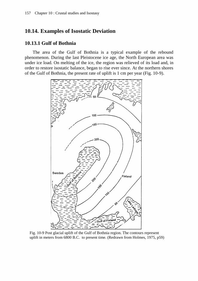
157 Chapter 10 : Crustal studies and Isostasy
10.14. Examples of Isostatic Deviation
10.13.1 Gulf of Bothnia
The area of the Gulf of Bothnia is a typical example of the rebound
phenomenon. During the last Pleistocene ice age, the North European area was
under ice load. On melting of the ice, the region was relieved of its load and, in
order to restore isostatic balance, began to rise ever since. At the northern shores
of the Gulf of Bothnia, the present rate of uplift is 1 cm per year (Fig. 10-9).
Fig. 10-9 Post glacial uplift of the Gulf of Bothnia region. The contours represent
uplift in meters from 6800 B.C. to present time. (Redrawn from Holmes, 1975, p59)

158
The isostatic anomaly over this area is found to be of negative value
reaching about -50 mgal at its centre. As it is explained above, this represents the
case of overcompensation which implies that the present size of the root is larger
than it is inferred from the elevation of the surface topography. The subsidence
caused by the ice-load was accompanied by lateral movement of the sub-crustal
material and the ice removal seems to have occurred too fast to an extent
whereby the readjustment process was not keeping pace with the ice removal
rate.
10.13.2 Rift Valleys
Rift valleys or grabens are tectonic features formed as result of a faulting
process creating a long strip of a subsided block bounded by normal faults. The
Great Rift Valley of East Africa, the Rhine Graben, the Mid-Atlantic Ridge Rift
are typical examples of such large-scale tectonic structures. These are thought to
be formed as a result of regional uplift associated with tension and rifting, a
process similar to that taking place with uplifted formations pushed by a growing
salt dome. The end result is a graben in which the inner sinking block is forming
a “root-like” mass-deficiency structure. This model furnishes adequate
interpretation for the negative isostatic anomalies normally found over these rift
valleys.
The African Rift Valley extends from the Zambezi northwards passing
through the Red Sea and the Dead Sea depressions. Across certain parts of this
Rift Valley it is found that the isostatic anomaly is of large negative values over
the central zone and small positive values over the surrounding rims. This
indicates that a density-deficient “root structure” must exist underneath the Rift
Valley at those locations (Fig. 10-10).
Fig. 10-10 Profiles across four of the African rift valleys with the corresponding gravity
isostatic anomalies determined by E. C. Bullard (1936). Redrawn from Fig. 773 in
Holmes, 1975. p. 1062.

159 Chapter 10 : Crustal studies and Isostasy
10.13.3 The Red Sea
Due to ocean floor spreading and crustal separation phenomenon, Arabia is
moving away from Africa forming an intervening gap which is the Red Sea
structural depression. The Red Sea is considered to be an extension to the
African Rift Valley since it is a graben-form depression bounded by normal
faults. However it differs from the African Rift in that it shows positive gravity
anomaly over its central part. From seismic data it was inferred that the Sialic
layer is missing in the zone bellow the Red Sea and it is replaced by intrusive
basic rocks which are of a higher density. Thus the presence of such high-density
rocks near the surface instead of the lighter Sialic rocks explains the positive
isostatic anomaly over the trough of the Red Sea (Fig. 10-11).
10.13.4 Ocean Deeps and Island Arcs
Large negative isostatic anomalies (less than –200 mgal) are found over a
belt that parallels approximately the ocean deeps near the East Indies,
Philippines Islands and Aleutian Islands. On both sides of the belts of the large
negative anomalies, positive isostatic anomalies are usually observed, especially
Fig. 10-11 Profile across the Red Sea (near its southern end) with the corresponding
gravity isostatic anomaly determined by R. W. Girdler (1958), redrawn from Fig. 787 in
Holmes, 1975. p. 1080.

160
on the side facing towards the continents. The amplitudes of these positive
anomalies are usually smaller than those of the negative anomaly belts.
10.13.5 Cyprus and Hawaii Islands
Large positive isostatic anomalies are observed over some restricted zones
of the earth crust. Examples of such zones are Cyprus (exceeding +150 mgal),
portions of Hawaii (exceeding +100 mgal) and Armenia (exceeding +100 mgal).
These represent cases of under compensation. This means that these structures
have no roots which are evidently supported by the rigidity of the crust rather
than being supported by the buoyancy effect.

Chapter 11
GRAVITY EXPLORATION RECENT DEVELOPMENTS
Throughout the 20th century, the classical geophysical exploration methods,
including the gravity method, were extensively applied in the search for mineral
and hydrocarbon deposits. Geophysical research has led to great progress in
instrument technology as well as in the other basic exploration elements.
Satellite radar-based positioning technique, computer hardware, and software
systems and all other modern supporting technologies (based principally on
modern digital electronics) have collectively contributed to the development of
the gravity method.
The main developments that occurred in the gravity exploration method
were in the airborne gravity, borehole gravity, and in geodetic studies. It is
useful to know that satellite-borne instruments cannot measure acceleration
while the satellite is in free fall. Satellite-based gravity information can be
indirectly inferred from the satellite altitude and its orbit shape.
Here-below, we shall give brief presentation on the basic fundamentals of
the airborne gravity and borehole gravity since these have their principal
application in the field of petroleum and mineral deposits.
11.1. Airborne Gravity
Airborne gravity measurements (or aerogravity, as it is referred to
sometimes) are concerned with measuring the acceleration due to the Earth’s
force of gravitational attraction by instruments carried by a moving airplane or
helicopter. In essence, the aerogravity observation includes measurements of the
acceleration vector, location, velocity vector, and altitude of the aircraft.
The main difficulties met with in airborne gravity surveys are introduced by
the too large and rapid changes in the measured gravity values caused by the
aircraft complex motion. During flight, this may experience a side-way, head-
way, and latitude changes. These effects are similar to those found in ship-borne

162
gravimetry, but with much slower changes. Compensation of these changes is
usually done in the processing stage.
Processing of the observational data involves compensation for aircraft
vertical motion, gravimeter platform velocity changes, Eotvos effect, free-air,
and latitude corrections. Residual random noise can be removed by applying a
low-pass filter. The processed data are usually downward continued to the
ground surface or to the sea level for interpolation and/or comparison with
conventionally recorded gravity data (Dobrin and Savit, 1988, p 556).
11.1.1 Aerogravity Basic Principles
In the stationary type of environment as in the case of land gravity
measurements, the measured gravity would be the effective acceleration vector
sensed at that position. In the airborne gravity, the sensed gravity is a
combination of the Earth gravitational acceleration component, in the direction
of the measuring gravimeter-axis, and all acceleration components created from
the aircraft motion. In the geophysical literature, these two types of acceleration
are usually termed the gravitational and the kinematic accelerations respectively.
Due to the aircraft complex motion, two problems need to be solved. These are
the gravimeter stabilization and isolation of the gravitational acceleration from
that created by the kinematic motion.
Schwartz and Li, (1997) and Wei, (1999) classified airborne gravimetry in
general into three types. These are:
- Scalar gravimetry
- Vector gravimetry
- Gravity gradiometry
(i) Scalar gravimetry
In scalar gravimetry, only the magnitude of the gravity vector is determined.
One way to accomplished this is with the use of the so-called Strapdown Inertial
Navigation System (SINS). This approach, called the Strapdown INS Scalar
Gravimetry (SISG) System, is concerned with measuring only the vertical
component of the gravity vector.
Another approach is based on the use of a triad of three orthogonal
accelerometers from which the gravity magnitude is determined by subtracting
the acceleration vector due to the aircraft motion from the measured acceleration

163 Chapter 11 : Gravity Exploration recent developments
vector. This system is normally referred to as the Rotation Invariant Scalar
Gravimetry (RISG) system.
(ii) Vector gravimetry
This type of gravimetry is concerned with determination of the full gravity
vector. This is accomplished by using inertial platform system, with which each
of the three components; one vertical and two horizontal components (Jekeli and
Kwon, 1999).
(iii) Gravity gradiometry
An arrangement of two gravimeters aligned on a common vertical axis can
give the vertical gradient of the gravitational field at the measurement location.
In airborne gravity gradiometry, the first derivative of the acceleration vertical
component (= the second derivative of the gravity potential) is measured.
Gravity-gradient measurement is normally evaluated in Eotvos units, where one
Eotvos is equal to 10-6 mgal/cm.
Gradiometry measuring instruments in common use (like the Falcon gravity
gradiometer) proved to be of higher accuracy and resolution compared with the
scalar and vector gravimetry, gradiometers. In an actual airborne gravity survey,
the flight was conducted along a grid of orthogonal flight-tracks spaced at about
2-5 km apart at an altitude of about (200-500) m above the mean terrain level
(Jekeli, 1993).
A comprehensive overview of gravity gradiometry is found in Bell et al,
(1997).
11.1.2 Aerogravity Main Objectives
Airborne gravity surveying aims at two main objectives. These are the
geodetic and geologic exploration studies of the Earth surface, based on the
airborne gravity measurements.

164
(i) Geodesy (local geod exploration)
The geoid (defined to be the equipotential surface of the gravity field) can be
represented by the mean sea level. Airborne gravity data have proved to give
highly accurate information on the local geodetic changes.
(i) Geology (regional geologic exploration)
In geophysical studies, airborne gravity is extensively applied in mapping
geological changes especially on the large-scale (regional) changes. The gravity
maps obtained from aerogravity surveys are compared and tied up with existing
conventional gravity data and interpreted to determine subsurface geological
structures. Structural and stratigraphic anomalies, with mineral and hydrocarbon
contents, can be explored by this fast, accurate, and cost effective technique.
11.1.3 Historical Development of Aerogravity
The first reported test of airborne gravity measurements was conducted in
the mid-1950s (Lundberg, 1957), where a system based on gravity gradiometry
was applied. Due to lack of the accurate navigation system and insufficient
technical control available then to avoid gravity interferences, the airborne
gravity, as an exploration tool, did not develop until the 1980s, when the
Differential Global Positioning System (GPS) was introduced. Since then, the
technique has experienced continuous improvements in both measurement-
accuracy and spatial resolution.
The major problems met with in the early experiments of airborne gravity
surveying were the aircraft navigation control, and lack of a gravimeter capable
of accurate measurements of acceleration changes in a dynamic environment.
However it is found that better accuracy is obtainable when using large aircraft
smoothly flying at high altitudes.
The tests carried out in the early 1960s were based on gravimeters installed
in fixed-wing aircrafts. In those experiments, the gravimeters used were
modified sea-gravimeters (developed by LaCoste and Romberg for ship-borne
gravity measurments) that use gimbal suspension to handle horizontal
acceleration changes. The first successful gravity measurement from a helicopter
was performed in 1965. In the following year, a more accurate helicopter-borne
test (of about 3 milligal) has been successfully performed. This test has led to the
development of a complete helicopter-borne gravity measuring system (HGMS).
The main advantages of a helicopter over a fixed-wing aircraft are lower altitude
and slower flight which are increase the spatial resolution.

165 Chapter 11 : Gravity Exploration recent developments
The break-through in the development of the aerogravity as an effective
exploration tool came at the end of the 1980s when the DGPS technology was
introduced. This highly advanced navigation system helped in accurate
measurement location and in developing gravimeter stabilization systems to
overcome those turbulences affecting the gravity measurements during flight.
One of the first large-scale airborne gravity surveys, with the application of these
developments, was conducted over Greenland in 1991 and 1992 by joint
cooperation between U.S Naval Research Laboratory and the Danish National
Survey. Other examples of such surveys were the airborne gravity surveys of
Switzerland in 1992 and over the West Antartic ice sheet in (1991-1997). After
these pioneering works many airborne gravity surveys were conducted with
reported accuracies of 1.5-2.0 milligal at 5-6 km spatial resolution. Examples of
these surveys are done over Malaysia (2002-2003), Mongolia (2004-2005),
Ethiopia (2006-2007), and Taiwan (2007). The information cited above is based
on the more detailed account presented by Alberts (2009, p7).
11.1.4 Advantages and Limitations of Airborne Gravimetry
The main advantages of airborne gravity exploration are the following: (i) Fast exploration tool, as it is possible to cover thousands of line kilometers in few
weeks survey-time. It is, therefore, suited for reconnaissance (regional
coverage) surveying rather than for detailed local investigations.
(ii) Capable of surveying inaccessible areas and territories which are hard to survey
with the conventional measuring tools, such as rugged mountains and iceberg
covered areas.
(iii) Providing uniform coverage of the gravity field measurements, where the
reading locations are independent of the terrain nature of the survey area.
(iv) Cost-effective exploration-technique in surveying large areas, due to being fast,
efficient, and using fully automated field procedure.
Corresponding to these advantages, airborne gravimeter surveys suffer from
a number of limitations. The principal limitation of the method is its need for
highly sophisticated equipment carried by a fixed-wing airplane or a helicopter.
This feature made the use of the technique restricted to a few number of
specialized exploration companies. The second important limitation is its
relatively low spatial-resolution that makes the technique more suited for large-
scale (regional) surveying rather than for detailed (local) geophysical
investigations.

166
11.1.5 Accuracy and Spatial Resolution of Airborne Gravimetry
In the geophysical literature, it is stated that acceleration changes due to
aircraft flight disturbances may reach as much as 0.1G (= 100 000 mgal). An
airborne gravimeter is required to measure gravity to better than one milligal. In
this noisy environment, a sufficiently accurate value for the vertical acceleration
is extracted by the appropriate measures taken in the design of the measuring
system.
In the early 1980s, measurement accuracy attained in airborne gravity was
estimated to be of 5 milligals (Brozena, 1984). With the more modern airborne
gravimetry systems, an accuracy of 1-2 milligals, at a 2-km spatial resolution has
been attained (Alberts, 2009). Airborne gravity measurements are of accuracy
and spatial resolution which are insufficient for detailed mineral exploration.
This limitation is believed to stay unresolved hindrance for being applied as a
detailed mineral exploration tool (van Kann, 2004).
The attainable resolution depends upon flight speed, survey-line grid,
elevation, sampling period, and type of the applied filter. Airborne gravity
surveys seem to be controversial; some geophysicists believe that for regional-
type surveys, airborne gravity can yield usable results. Others have reported that
inconsistent results were obtained when airborne and ground surveys were
compared after allowance was made for elevation differences. The magnitude of
this error was greater than the internal precision of most airborne gravity systems
(Dobrin and Savit, 1988, p 557).
11.1.6 Processing of the Aerogravity Data
In essence, processing of the aerogravity measurement data is to remove all
non-gravitational acceleration components from the total gravimeter
measurement acceleration. Due to the complex aircraft motion, the computation
of the non-gravitational components becomes much more complicated than that
involved in the case of the traditional ground gravity surveying data. Especially
designed software systems are applied in the data processing.
The Main Corrections
The main corrections done for the gravimeter reading involve subtraction of
acceleration components due to aircraft motion, Eotvos correction, tilt correction
due to non-level position of the measuring system, and the normal gravity. For
the free-air gravity, a term, which is a function of the elevation and geoid

167 Chapter 11 : Gravity Exploration recent developments
undulation, is added. Finally, the Bouguer anomaly is computed based on the
available density model.
Over the survey time, a number of airborne base readings are normally made
to construct the gravimeter drift function which is used for the drift correction. A
land-based gravimeter, tied to absolute gravity stations, is used to establish the
reference gravity values. Certain measures are applied to determine the
calibration factor of the measuring accelerometers.
Data Filtering
Airborne gravity measurements are made in very dynamic operation
conditions in which high-frequency, large-energy levels are introduced in the
readings. Typically, noise-to-signal ratios of 1000 or more can be observed
(Schwartz and Li, 1997). In such an environment, resolving of the gravity signal
forms a serious problem in aerogravity surveying. To extract the useful gravity
signal from such a high-noise record, a low-pass filter is usually applied.
Low-pass filtering forms an important feature of the airborne gravity
processing. The main purpose of the filtering is to remove the high frequency
gravity noise which is usually present in the gravity measured record, obscuring
the gravity anomaly signal. Low-pass filtering forms an important feature of the
airborne gravity processing. The main purpose of the filtering is to remove the
high frequency gravity noise which is usually present in the gravity measured
record, obscuring the gravity anomaly signal.
Modern gravity-data interpretation work is mostly using inverse and forward
modeling techniques (Jacobi and Smilde, 2009)
Airborne Gravity versus Land Gravity
Comparison of the airborne gravity data with the traditional land-surface
gravity data can give an evaluation measure to aerogravity as a geophysical
exploration tool. In general, it is found that a small constant offset-shift is
existing between the airborne gravity map and the corresponding ground gravity
map. For comparison purposes, this offset is removed by a bulk-shift of the
airborne data.
There are two ways to tie airborne- and ground- gravity maps. The simple
way is to add the average of the gravity differences found at the grid points to
the airborne gravity map, and the other way is to upward continue of the ground

168
gravity data to the aircraft mean flying level. By subtraction, the mean difference
between the two types of survey can be calculated.
To assess the accuracy of airborne gravity surveying, a comparative study is
made on an area for which airborne gravity and ground gravity data are available
(Elieff, 2003). In this study, a comparison was made between the airborne
gravity data with the upward continued ground data, giving a standard deviation
of 0.62 mgal (for the differences between air gravity and ground readings) at
flight level, in addition to a constant offset-shift of 1.4 mgal between the air- and
ground-data.
At present, airborne gravity surveying is claimed to achieve accuracies of
about 0.5 mgal with spatial resolution of 2-4 km, and is compared favorably with
most ground gravity data sets. The following figure (published by Fugro on its
web site) shows the correspondence between the results of traditional ground
gravimetry (A), the airborne conventional gravimetry (B), and the airborne
gravity gradiometry (C).
It is clear from this example that the airborne gravity map is in remarkable
coincidence with the ground-gravity map. The almost perfectly matching results
of the airborne gravity map, compared with that obtained from the standard
ground gravity surveying, strongly support the reliability and compatibility of
the modern aerogravity. Further, the gradiometry map shows, as expected,
A Ground Gravimetry 500 m to 5 km stations
B Airborne Gravimeter 4 km Line spacing
C Airborne Gravity
Gradiometry 1 km Line spacing

169 Chapter 11 : Gravity Exploration recent developments
improved resolution-power compared with the airborne and conventional ground
gravity measurements.
11.2. Borehole Gravity
Borehole gravity is concerned with measuring the gravity variation down a
drilled hole. The measurement instrument is a specially designed gravity logging
sonde (the borehole gravity meter, BHGM) which can measure the gravity
variation with depth. The BHGM technology, considered to be part of the micro-
gravity exploration, was developed by the well known LaCoste & Romberg Inc.
into an efficient and reliable geophysical exploration tool capable of detecting
changes in density and porosity of geological formations in addition to reservoir
monitoring and mapping of structural anomalies such as salt domes and reef
deposits.
As early as 1950s, scientific papers were published in the geophysical
literature dealing with the borehole gravity in detail, as for example, (Smith,
1950) and (LaFehr, 1983).
11.2.1 Principles of Borehole Gravity
The geophysical principles of this method are based on the direct
relationship connecting the gravity changes with the density contrast. The
measured change in density is a function of the vertical gradient of gravity. Thus,
a density measurement requires measuring gravity at two different depths. Since
the expected changes in gravity are very small, the borehole gravity sensor is
required to be very sensitive measuring instruments. Accuracy of the produced
density values depends on the accuracy of the corresponding gravity and depth
readings.
11.2.2 Operational Considerations
The measuring meter is effectively, a very sensitive spring balance which
measures changes in gravitational force acting on the mass attached to its spring.
Since the sensing mass is constant, the changes are expressing the gravity
(acceleration) changes.
Logging operation is similar to the procedure followed in well velocity
surveying. The measurement tool is stopped at the planned depth levels at which
BHGM readings are taken. The borehole must not be deviating from the vertical

170
by more than that defined for the measuring system, and the meter, which is well
thermostat-controlled, needs to be leveled at each measurement station.
The vertical resolution obtained depends on the discrete depth intervals
adopted for the measurements.
11.2.3 Advantages and Disadvantages of Borehole Gravity
The borehole gravity logging is a passive exploration tool, in the sense that
it does not require any artificial energy source. Further, the produced gravity log
can be directly interpreted in terms of density variation with depth. This logging
tool has the merit of being unaffected by the borehole conditions, such as poor
cementing, washout, and fluid invasion. The logging process can be carried out
in case, as well as in open holes.
With an available gamma-ray log, porosity and nature of pore fluid (gas or
liquid), in addition to density variations can be determined.
11.2.4 Scope of Applications
There are two main fields of application of the BHGM logging work. These
are the close-up sensing of formation rock density (down-hole density logging)
and the remote-sensing of neighboring geological structures. Borehole gravity
logs can give useful information on density and porosity variation as well as
detection of types of bore fluids and hence contribute to reservoir evaluation
studies. Coupled with gamma-ray logging data the technique can give important
information on the anomalous geological structures found in the vicinity of the
logged section. In this context, structures of sufficiently high density contrast,
like salt domes and reef deposits, can be detected by BHGM.

Chapter 12
CASE HISTORY OF GRAVITY SURVEYS
In this chapter, we shall present two actual surveys carried out by the authors.
The first one was carried out by Dr. Hamid N. Al-Sadi in the County of Devonshire,
England (Al-Sadi, 1967) and other survey was carried out jointly by Zuhair. D. Al-
Shaikh and Ezzadin N. Baban in Iraqi territories (Z.D. Al-Shaikh and E.N. Baban,
1991).
(A) GRAVITY SURVEY IN ENGLAND BY AL-SADI, 1967
12.1. Location of the Survey Area
The survey area (8 x 12 mile2) is located in the extreme North-Western corner
of Devonshire in England (Fig. 12-1). The latitude 51° 05' N and the longitude 3° 55'
W form the southern and eastern boundaries of the area respectively. The ground
elevation lies in the range 900-1000 feet above sea level. There is a gradual decrease
in elevation level in the western and South Western direction.
Fig. 12-1 Location map of the survey (North Devon, England)

172
The survey was carried out in the summer of 1965 using a Warden gravimeter.
There was no need for conducting a topographic survey for the survey-area since a
large number of station points (bench marks and spot heights of known elevation)
exist at an adequate coverage-density throughout the area.
12.2. Geological Structure of the Survey Area
All of the outcropping rocks are of Devonian age, with the oldest rock of the
sequence is found on the north coast of the area. The Lower Devonian consists of
coarse arenaceous rocks with shaly or slaty beds. The Middle Devonian consists of
slates within which there are two 30-foot bands of limestone. The Upper Devonian
is dominantly made up of slates and sandstones that include the outcropping
Pickwell Down Sandstone member which was mainly investigated in this case-
study.
The succession of the Devonian rocks forms parallel tracts striking at bearing of
about 285° with an average dip of 35° due south. The axial planes of folds are
parallel to that of the synclinorium of which North Devon is part-of. The fold axes
are generally pitching 15° - 30° due west.
12.3. The Field-Work
12.3.1 Measurement Instrument
A Worden gravimeter was used in the survey. The instrument is housed in an
evacuated chamber (thermo flask) with a built-in temperature-compensating device.
Instrument reading is made by observing an illuminated index-fiber through a built-
in microscope which is provided with a hair-line eyepiece for viewing the scale
changes.
12.3.2 Instrument Calibration
The gravimeter, used in this survey, has been previously calibrated by the
instrument makers. The determined calibration factor was (0.4240) mgals/scale
division. The instrument was re-calibrated before the start of the survey by taking
readings at two points at which the gravity value is accurately known. From dividing
the difference in gravity value by the difference in the corresponding dial-readings,
the scale factor is obtained. The scale factor 0.4240 mgal/s.d was confirmed by this
experiment and thus was adopted in the reduction of readings of this survey.

173 Chapter 12 : Case history of gravity surveys
12.3.3 Instrument Drift
As a first step of the survey, the curve of the drift characteristics of the
gravimeter is constructed. As it was explained, the instrumental drift is due mainly
to three causes. These are the slow plastic deformation, thermal expansion in the
instrument components due to the Earth tidal effect. To determine the drift
characteristics, the gravimeter was set up at a location and read at frequent intervals
for several hours. The mean drift rate was determined from the established drift-
curve and found to be within the range of 0.03-0.04 mgal/hour. These figures serve
as guide for giving an idea about the degree of stability of the instrument used in the
survey. However, the drift has been accurately computed alongside the survey
readings and allowed for gravity value determination be done in the data reduction
stage. The established drift curve has shown that the drift is linear over 2-3 hours
time-span. This information was made use of in conducting the survey as explained
below.
12.3.4 Instrument Set-Up
The slightly concaved tray, on which the gravimeter rests, is placed on the spot
where a reading is to be taken. The bull’s eye spirit level found at the center of the
tray indicates the leveling state of the tray which is firmly placed on the ground. The
gravimeter is then placed on the tray and accurately leveled at each station reading.
12.3.5 Instrument Reading
To read the gravimeter, after being properly set-up over its base-tray, the light
of the scale dial is switched on and the beam is brought to the null-position using the
torsion screw of the instrument. Before taking the reading, the instrument levels are
checked and the index beam is viewed again to make sure that it is still in the null
position. The reading is then taken to a precision of 0.1 scale-division by reading the
verniere scale of the gravimeter after restoration of the illuminated index-fiber to the
null position..
12.4. The Base-Station Network
The second step in conducting the gravity survey, after calibration and drift
determination of the gravimeter, is the establishment of the base-station network. A
base station is defined to be that point which is accurately located within the survey-
area, at which the gravity value is precisely known. The base-station serves two
purposes; first it is used as a reference point for computing gravity value at other

174
station-points from reading gravity differences. The second purpose is the determination of drift changes which take place during the survey-work. This is
done by taking repeated gravity-readings at the base station at different time-
intervals.
12.4.1 Base-Station Network Establishment
In this survey area, eight well-spaced base-stations (B1, B2, …, B8) were
established (Fig. 12-2).
The main base station (B1) at which the absolute gravity value is already known
(= 981192.35 mgal) is located near Barnstaple town, whose coordinates are 51° 04'
12'' N for its latitude and 04° 04' 24''W for its longitude.

175 Chapter 12 : Case history of gravity surveys
Starting with the reference base station (B1), the second base station (B2) and
the rest of the eight base stations are established by taking readings in the following
sequence:
The actual readings (taken on the 26th of June, 1965) are shown in the following
table:
From the drift curve (shown in the first column of this table), the drift value is
determined and the true gravity difference between B1 and B2 is found and then
after being converted into milligals (using the conversion factor 0.424 mgal/s.d) the
gravity value of B2 is determined. Now B2 can be used as a new reference base
station in computing another base station such as B3. This procedure is repeated to
establish the rest of the base stations (B4, B5, B6, B7, and B8).
12.4.2 Closing-Error Distribution
In this survey, the base stations (B1, B2, B3, B4, B5, B6, B7, & B8) were
connected by four loops (compartments). The four closing errors in these loops were
determined and found to be -0.11, +0.62, -0.48 and -0.63 scale-division. These
B1 B2 B1 B2 B3 B2 B3 B4
Drift
curves
Base-
station
Gravimeter
reading (s.d.)
Time of reading (hour: minute)
B1
B2
B1
B2
Gravity reading
Time of
reading
544.2
566.9
544.0
566.6
18 : 21
19: 10
19 : 28
19 : 55

176
closing errors are distributed among the eight base stations. A simple method of
closing-error distribution (explained here-below) is done by assigning an error-
variable for each polygon-side and then solving simultaneous equations. The
procedure can be explained as follows:
In this survey, we have four compartments (A, B, C, & D). For each free side a
variable was assigned. The variable (a) was assigned for the free sides of the first
polygon (A), b for the second polygon (B) and so on. For the common sides, assign
differences, (a-b) for the side which is common between polygons A & B, (b-c) for
the side which is common between polygons B & C, and so on as shown in (Fig. 12-
3).
An equation of each polygon is obtained from equating its closing error to the
algebraic sum of the variables of its sides. The following four simultaneous
equations are then obtained:
4a - b-d = - 0.11
Fig. 12-3 Base-station network (forming four compartments) with the
computed closing-error values (a, b, c, d). Arrow direction indicates relative
increase in gravity value between base stations.

177 Chapter 12 : Case history of gravity surveys
4b - a- c - d = + 0.62 4c - b = - 0.48
3d – a - b = - 0.63
Solution of this set of equations gives:
a = - 0.0657 b = + 0.0592 c = - 0.1052 d = - 0.2122
The correction in milligals per each side is thus determined by using the
conversion factor (0.424 mgal/s.d.), and reversing the algebraic sign of each of the
correction values. Fixing the main base-station (B1) at its given value (981192.35
mgal), the adjusted values of the other seven base-stations are finally determined.
The whole process is summarized in the following table:
Polygon side
Original difference
(s.d)
Correction (s.d)
Corrected difference
(s.d)
Corrected difference
(mgal)
Corrected Base-Station gravity (mgal)
B1-B2 +22.82 +0.066 +22.89 +9.71 B1= 981192.35
B2-B3 -55.55 +0.066 -55.48 -23.52 B2= 981202.06
B3-B4 +0.68 +0.125 +0.81 +0.34 B3= 981178.54
B4-B1 +31.94 -0.147 +31.79 +13.48 B4= 981178.88
B3-B6 -52.20 -0.059 -52.26 -22.16 B5= 981172.27
B6-B5 +37.63 -0.164 +37.47 +15.89 B6= 981156.38
B5-B4 +15.87 -0.271 +15.60 +6.61 B7= 981146.61
B5-B1 +47.18 +0.212 +47.39 +20.09 B8= 981162.03
B6-B7 -23.15 +0.105 -23.05 -9.77
B7-B8 +36.25 +0.105 +36.36 +15.42
B8-B5 +24.05 +0.105 +24.16 +10.24
The last column of the above table contains the adjusted gravity values of the
base stations used in this survey. The main base station B1 (having gravity value of
981192.35 milligal) was made as reference point to which the other gravity values
(B2, B3,…,B8) were corrected. As shown in the above table, the corrected
differences read over each of the lines connecting the base-stations were used in the
correction process.. This process (called base-station tie-up) furnished eight base
stations that are well distributed throughout the area.

178
To further clarify the correction process let us explain the procedure followed in
calculating the closing error in the first compartment (compartment-A) formed by
the loop (B1 B2 B3 B4). This is done as follows:
Let the difference between station B1 and station B2 be diff.1, between B2 and
B3 to be diff.2, between B3 and B4 to be diff.3, between B4 and B1 to be diff.4. The
closing error is then found by summing diff.1 + diff.2 + diff.3 + diff.4 algebraically.
In the same way, the closing errors in the rest of the compartments are found and
converted into gravity units using the conversion factor (0.424 mgal/s.d).
The closing errors in the four compartments were found to be -0.047, +0.263, -
0.204, and -0.267 mgals, giving a mean absolute closing error of 0.195 mgal, and
standard deviation of ±0.174 mgals. These residual errors were distributed over the
gravity values of the base stations. Fixing the main (reference) base station (B1) at
the value of 981192.35 mgal, the adjusted values of the other seven bases became as
follows:
12.5. Station Reading
Once the base-station network is established, a systematic field procedure is
followed to execute gravity measurements at all station-points in the survey area.
The daily work is normally started and ended by taking a reading at a reference
base-station. Both of the gravity reading and its reading-time are documented. This
process (reading and documenting the gravimeter reading and the time of the
reading) is repeated at each of the survey station-point. Readings at the base station
are repeated at about two-hour intervals throughout the working day.
Station-points of this survey are not uniformly distributed in the survey area.
There was no need to establish a uniform station-grid, since an adequate number of
station-points of known x, y, z -coordinates was available over the whole area. The
Base- Station
Location name
Latitude (N)
Longitude (W)
Adjusted gravity (mgal)
B1 Barnstaple 51° 04' 12'' 04° 04' 24'' 981 192.35
B2 Braunton 51° 06' 10'' 04° 09' 25'' 981 202.06
B3 West Down 51° 09' 34'' 04° 07' 24'' 981 178.53
B4 Marwood 51° 07' 05'' 04° 04' 39'' 981 178.87
B5 Shirwell 51° 07' 04'' 04° 00' 16'' 981 172.25
B6 Berry Down 51° 10' 29'' 04° 02' 37'' 981 156.37
B7 Wistlandpound 51° 09' 50'' 03° 56' 19'' 981 146.60
B8 Bratton Fleming 51° 07' 11'' 03° 56' 35'' 981 162.01

179 Chapter 12 : Case history of gravity surveys
following table shows a sample data-sheet in which the data set was read and
documented on the 23rd of June, 1965.
Station seq. no
Longitude (W)
Latitude (N)
Elevation (Feet)
Time (h-min)
Reading (s.d)
Drift (s.d)
Gravity Reading (drift-corrected) (s.d.) (mgal)
B4 04° 04' 39'' 51° 07' 05'' 384.5 14 - 22 503.4 0.0 503.4 178.87
7 04° 02' 11'' 51° 08' 54'' 826.6 14 - 57 448.4 0.0 448.4 155.55
8 04° 01' 23'' 51° 08' 53'' 852.0 15 - 12 444.5 0.0 444.5 153.90
9 04° 01' 46'' 51° 08' 52'' 849.7 15 - 26 444.4 0.0 444.4 153.85
10 04° 01' 30'' 51° 08' 51'' 804.0 15 - 40 449.5 0.0 449.5 156.02
11 04° 01' 28'' 51° 08' 41'' 810.0 15 - 54 448.8 0.0 448.8 155.72
12 04° 01' 26'' 51° 08' 35'' 821.5 16 - 04 446.7 0.0 446.7 154.83
13 04° 01' 14'' 51° 08' 26'' 756.4 16 - 14 452.7 0.0 452.7 157.37
B4 04° 04' 39'' 51° 07' 05'' 384.5 16 - 37 503.4 0.0 503.4 178.87
14 04° 01' 07'' 51° 08' 09'' 723.2 17 - 14 453.9 0.0 453.9 157.88
15 04° 01' 07'' 51° 08' 01'' 717.0 17 - 31 453.5 0.0 453.5 157.71
16 04° 01' 03'' 51° 07' 52'' 663.0 17 - 40 460.0 -0.1 459.9 160.43
17 04° 00' 57'' 51° 07' 40'' 577.5 17 - 55 471.8 -0.1 471.7 165.43
B4 04° 04' 39'' 51° 07' 05'' 384.5 18 - 27 503.5 -0.1 503.4 178.87
The first column in this table contains the sequence number, and the following
three columns contain the x y z coordinates of the station points. Columns 5 and 6
are assigned for time and gravimeter-readings respectively. The rest of the columns
contain the data-reduction results, where the last column shows the final drift-
corrected gravity value in milligals. Conversion to milligals is achieved through
multiplication by the scaling factor (0.4240 mgal/s.d).
12.6. Reduction of Field-Data
Data reduction (Data processing) of field data involves a sequence of
corrections applied to reduce the field-data to the final Bouguer gravity values. To
achieve this objective, the following corrections were applied:
(i) Drift Application and Reading Conversion
The instrumental drift is determined from the repeated readings made at the
concerned base-station over time-spans which, in this survey, were about two hours.
Readings, after being corrected for drift, were then converted into milligals using the
instrument calibration factor which was 0.424 milligals/scale division.

180
(ii) Latitude Correction
This correction removes the gravity change (systematic increase in equator-to-
poles direction) due to flattening and rotation of the Earth. In this survey, the
correction is done by measuring the latitude of each observation point to the nearest
second and the corresponding theoretical gravity value (as given by the International
Formula) was read, and then subtracted from the observed gravity for each station of
the survey. It is be noted that the whole survey area is located between latitudes 51°
05` 44`` N and 51° 12` 32`` N.
(iii) Combined Elevation Correction
This includes the combined effect for the Free-Air and Bouguer corrections.
The formula for the combined elevation correction (CEC) is given by:
CEC = 0.09406 - 0.01276 * density milligal/foot
In this survey, the density value used for the Bouguer correction was 2.7 gm/cc.
With this value, the combined correction was found to be of 0.05961 milligals per
foot of station elevation.
(iv) Terrain Correction
Both hills above a station-level and valleys below have positive terrain-
corrections on the gravity value at that station. The correction per each station was
calculated by a computer program (Bott, 1959). The input data consists of location-
coordinates, elevations of station-points, mean density and relief information of the
area. The input data for the correction included areas that extend beyond limits of
the survey area in order to insure adequate correction for those stations located on
the outer fringes. Thus, the survey area was subdivided into (1km x 1km) squares
forming a total of 768 squares). In addition, a surrounding 8 km-wide strip was
included in the computation and was subdivided into (4km x 4km) squares (total of
72) and a second strip immediately beyond this of about the same width was also
divided into 8km x 8km squares. The average elevation of the topography in each
square (1x1, 4x4, and 8x8 dimensions) was manually estimated. The value (2.70
gm/cc) was used for the mean rock density.
By carrying these corrections, the gravimeter reading at each station in the
survey area was reduced to give the final Bouguer gravity anomaly in milligals.
These values are then posted on the base map of the area and finally presented as a
contour map (Fig. 12-4) ready for the next phase of the project which is the
interpretation process.

181 Chapter 12 : Case history of gravity surveys
Fig. 12-4 Bouguer anomaly map of North Devon-England, drawn at one-milligal
contour intervals (Al-Sadi, 1967).
12.7. Interpretation
Interpretation of the final Bouguer gravity map forms the ultimate aim of any
gravity survey project. In short, this phase of the survey gives the geological
structural model which is nearest to the realistic picture of the subsurface geology of
the area. The input data to the interpretation process is the Bouguer anomaly map
(shown in Fig 12-4) which was drawn at one-milligal intervals.
There are two types of approach for interpretation. These are qualitative and
quantitative approaches. After a descriptive approach and trying to associate the
main apparent changes with the available geological knowledge of the area, a more
deterministic approach is followed. This includes computations of the regional and
residual gravity then gravity-to-geology translation using model-analysis technique.

182
(i) Qualitative Approach
A visual inspection of this map revealed that the anomalies show a fairly
constant strike, which follows the trend of the Devonian outcrop very closely. In
addition, there exists a central region of anomaly disturbance. In general, the gravity
values are noted to be falling in a northerly direction. The Bouguer contour map (Fig
12-4) reveals a remarkable resemblance between the gravity picture and that of the
known geological structure of the area. In particular there is a close coincidence
between the central gravity-low and the outcrop of one of the Upper-Devonian
sedimentary members (the Pickwell Down Sandstone).
(ii) Quantitative Approach
Based on the general contour appearance and on the known geological structure
of the area, the gravity map was considered as being reflecting a two-dimensional
geological model consisting of parallel rock-layers dipping in a southerly direction.
For this reason, interpretation was based on drawing gravity-profiles perpendicular
to strike of the geological layers. To simplify the quantitative interpretation, regional
and residual anomalies are determined for the derived profiles rather than for the
whole contour map.
The Regional Gravity Anomaly
Due to the simplicity of the Bouguer gravity map, a manual method was used
in establishing the regional anomaly. Based on the analysis of ten profiles taken at
right angles to the general trend, it was found that the mean regional gradient is 1.2
± 0.20 mgals per mile. With this gradient the regional gravity is generally decreasing
in a northerly direction which was found to be in close agreement with the
assumption of thickening of the Carboniferous sediments which is separated from
the outcropping Devonian rocks by an assumed thrust zone. For a density contrast of
-0.15 gm/cc, these sediments must reach a thickness of about 3 miles at the northern
coast of Devon to account for the 30-milligal gravity change over the area.
The Residual Gravity Anomaly
The separated residual-anomaly profiles were subjected to model analysis.
These analyses have shown that they are caused by the dipping belt of sandstone
(the Pickwell Down Sandstone) and that the dip angle of the formation decreases
with depth. At a depth of about two miles, the formation becomes nearly horizontal.
Alternatively, it may terminate against an assumed thrust plane underlying the whole
Devonian beds. A typical profile is shown in Fig. 12-5.

183 Chapter 12 : Case history of gravity surveys

184
(B) GRAVITY SURVEY IN IRAQ BY Z.D. Al-Shaikh and E.N. Baban, 1991, J.Sci.Nat. 1(1A), 28-34.
POSSIBLE TRIASSIC FOLDING BELOW ABU RASSAIN, THE
WESTERN DESERT, IRAQ
12.8. INTRODUCTION
The area of study is situated in the west of Iraq, a few kilometers to the west of
the town of Hatra (Fig.12.6). It is a flat lying country except for sporadic hills such
as Kurat Tayarat.The area as a whole has a regional inclination towards the east and
northeast.
The surface geology is made up of Middle Miocene Lower Fars Formation
(cycles of clay, marl, limestone and gypsum) followed by the Upper Miocene Upper
Fars (sandstone, siltstone and clays). The well Khleisia-1(Kh-1) (350 20' northing,
41044' easting) gives the thickness of the L. Fars to be 550m while that of the U.Fars
200m. The deeper geological information is obtained from Kh-1 which penetrates
the succession to the Ordovician at a depth of3731.7m. Two other deep wells are
also used, namely Tel Hajar-I to the north (360 06' northing 41039' easting), which
penetrates to the Upper Triassic, and Ana-2 to the south (34° 22' northing, 41028'
easting), which penetrates to the Lower Jurassic. Correlating the various successions
between these wells shows that the Silurian is missing at Kh-1 due to uplift and
erosion during the late Ordovician and early Devonian. The succession from the
Upper Carboniferous to the Middle Triassic is also missing due probably to the
Hercynian orogeny. Kh-1 and Ana-2 show, furthermore, that the succession from the
Middle Jurassic up to the Upper Cretaceous is missing because of the uplifting
during the Kimmerian orogeny. The Alpine movement has also caused the removal
of the Palaeocene to the Middle Eocene in the area.
Tectonically, the area lies within the Hatra Uplift which belongs to the near
platform flank of the foredeep (Ditmar,1971). It has been subjected to successive
uplifting during different periods of its geological evolution. On the surface, only
few local anticlines exist among which Tayarat anticline is prominent in the
southwest of the area. It forms elongated hills stretching in a NE-SW direction for
some 20 kms.
Previously, the area was covered by gravity survey (Sayyab et. al., 1968) and by
aeromagnetic survey in 1978. Mohammed (1981) has studied a detailed seismic
reflection survey over the area and produced a topographical map of the basement
and an isopach map of the Lower Paleozoic rocks.

185 Chapter 12 : Case history of gravity surveys
Fig. 12.6 Location and Geological maps of the area.
In the following analysis, gravity features of local nature observed on the
gravity map will be concentrated upon.
12.9. PROCEDURE
The Bouguer anomaly map was prepared by Iraqi Petroleum Company (IPC)
with 1:200000 scale and a contour interval of one milligal is used (Fig. 2). It is
dominated by a large oval positive anomaly occurring in the middle of the area. It
has a sharp northern gradient with the well Kh-1lying in the middle of it. The
southern and eastern gradients are gentler. Its westerly extensions believed to run to
considerable distance into the Syrian territory Superimposed on this main anomaly
are sharp anomalies of various shapes and dimensions. One important anomaly of
these is the elongated one which extends from the town of Hatra to the southwest for
a considerable distance. Other local disturbances can also be seen.
To separate out local anomalies from the regional ones, smoothing procedure is
used. The smoothing procedure is carried out by profiles. Two sets of profiles east-
west and north-south) are taken on the map of Fig. 2. Smoothing regional field is
assumed for each profile. The intersection points serve as control over the regional
field taken. Using this procedure the smooth regional map of Fig. 3 is produced. It
shows the oval gravity "high" in the middle having a sharp gradient (reaching 0.6
rngal/km) toward the north. It has a maximum amplitude of 20 mgal and a half-
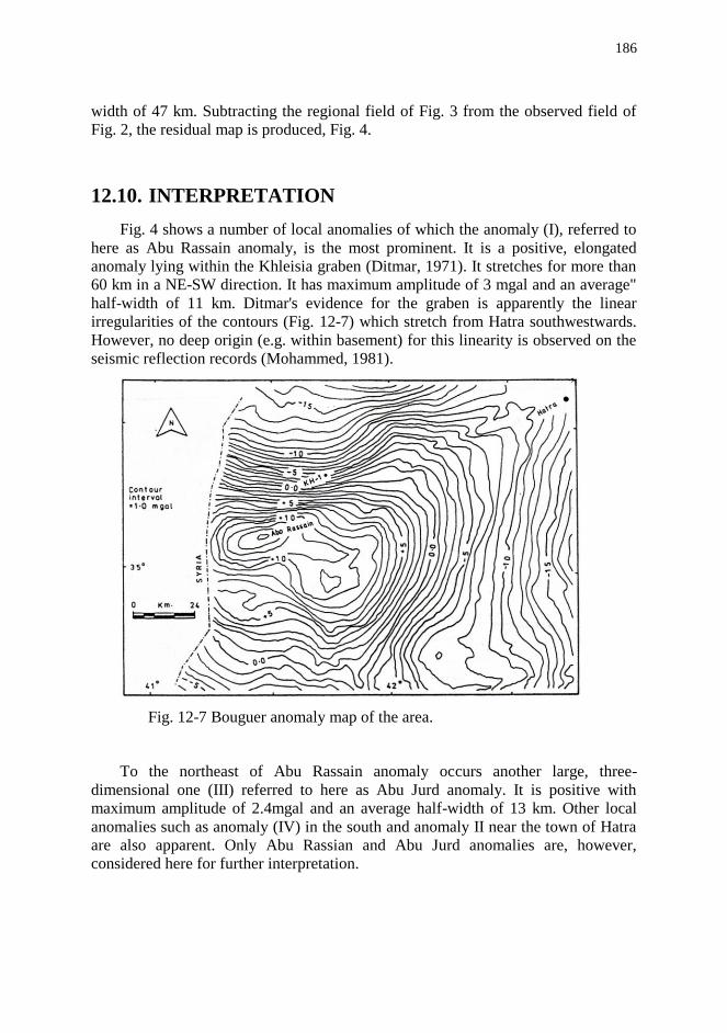
186
width of 47 km. Subtracting the regional field of Fig. 3 from the observed field of
Fig. 2, the residual map is produced, Fig. 4.
12.10. INTERPRETATION
Fig. 4 shows a number of local anomalies of which the anomaly (I), referred to
here as Abu Rassain anomaly, is the most prominent. It is a positive, elongated
anomaly lying within the Khleisia graben (Ditmar, 1971). It stretches for more than
60 km in a NE-SW direction. It has maximum amplitude of 3 mgal and an average"
half-width of 11 km. Ditmar's evidence for the graben is apparently the linear
irregularities of the contours (Fig. 12-7) which stretch from Hatra southwestwards.
However, no deep origin (e.g. within basement) for this linearity is observed on the
seismic reflection records (Mohammed, 1981).
Fig. 12-7 Bouguer anomaly map of the area.
To the northeast of Abu Rassain anomaly occurs another large, three-
dimensional one (III) referred to here as Abu Jurd anomaly. It is positive with
maximum amplitude of 2.4mgal and an average half-width of 13 km. Other local
anomalies such as anomaly (IV) in the south and anomaly II near the town of Hatra
are also apparent. Only Abu Rassian and Abu Jurd anomalies are, however,
considered here for further interpretation.

187 Chapter 12 : Case history of gravity surveys
Fig. 12-8 Regional anomaly map of the area.
To locate the source of these anomalies, a density contrast within the succession
of the wells referred to above is Kh-1 well which shows that an unconformity
surface exists on top of the Upper Triassic, so that the succession involving rocks
from the Middle Jurassic up to the Middle Cretaceous is missing. It is possible that
even the Lower Jurassic may be missing below the positive anomalies as the well
Kh-1 occurs only on the side of the anomaly and not at its culmination (see Fig. 12-
7). No information is available regarding direct and detailed density measurements
of the rocks involved in the western desert. However, Ditmar (1971) gave the
average density of the systems of the geological column in the western desert as
follows:
System Average density (gm.cm-3)
Middle & Lower Miocene 2.64
Palaeogene - Middle Cretaceous
2.46
Lower Cretaceous 2.61
Jurassic-Upper Triassic 2.71
Middle Triassic-Cambrian 2.62
If this table is considered for a density boundary, it can be seen that such a
boundary occurs between the Jurassic and the Cretaceous. A value of the density
contrast of 0.18 gm.cm-3 seems to exist between the Jurassic and the lower
succession on one side and the upper succession on the other. This contrast is similar
to that used by Mohammed (1981) to interpret the local anomalies in the

188
southwestern desert and is near enough the value used by Abass et. al., (1982) who
used 0.2 gm.cm-3 to interpret anomalies in the Hit-Shthatha area, the western desert.
Furthermore, referring to Fig.12-7 and noting the position of Kh-1 which shows only
a small thickness of L. Jurassic, it is believed that these rocks may further be
removed on top of the structure below the anomaly maximum. Therefore, a contrast
of 0.18 gm.cm-3 is considered representative for the difference between the Triassic
(Kurra Chine Formation) and the later succession.
Fig. 12-9 Residual anomaly map of the area
A. Abu Rassain anomaly
Figs. 12-9, 12-10 and 12-11 show the Bouguer anomaly profiles. Slightly
inclined regional gradient towards the northwest is chosen. Obviously, this
inclination is not taken in account by the smoothing procedure of the observed
contours. This slight "extra" regional effect is subtracted from the observed curve to
yield a simple "high" over the uplift. The best cross-section of the uplift was found
by trial and error using a computer program to compute the theoretical values of
gravity of two-dimensional models
The suggested model is an elongated uplift whose topmost rocks are made up of
Upper Triassic. The uplift is not symmetrical with the northern limb having greater
inclination. It is possible that the northern limb is faulted hence becoming steeper.
The top surface of the model along the profiles AA, BB, CC and DD occurs at
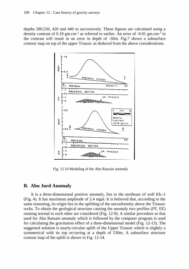
189 Chapter 12 : Case history of gravity surveys
depths 580,550, 420 and 440 m successively. These figures are calculated using a
density contrast of 0.18 gm.cm-3 as referred to earlier. An error of -0.01 gm.cm-3 in
the contrast will result in an error in depth of -50m. Fig.7 shows a subsurface
contour map on top of the upper Triassic as deduced from the above considerations.
Fig. 12.10 Modeling of the Abu Rassain anomaly
B. Abu Jurd Anomaly
It is a three-dimensional positive anomaly, lies to the northeast of well Kh.-1
(Fig. 4). It has maximum amplitude of 2.4 mgal. It is believed that, according to the
same reasoning, its origin lies in the uplifting of the unconformity above the Triassic
rocks. To obtain the geological structure causing the anomaly two profiles (FF, EE)
running normal to each other are considered (Fig. 12-9). A similar procedure as that
used for Abu Rassain anomaly which is followed by the computer program is used
for calculating the gravitation effect of a three-dimensional model (Fig. 12-13). The
suggested solution is nearly-circular uplift of the Upper Triassic which is slightly a
symmetrical with its top occurring at a depth of 530m. A subsurface structure
contour map of the uplift is shown in Fig. 12-14.
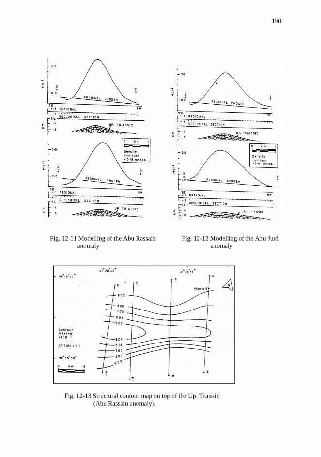
190
Fig. 12-11 Modelling of the Abu Rassain Fig. 12-12 Modelling of the Abu Jurd
anomaly anomaly
Fig. 12-13 Structural contour map on top of the Up. Traissic
(Abu Rassain anomaly).

191 Chapter 12 : Case history of gravity surveys
Fig. 12-14 Structural contour map on top of the Up. Traissic
(Abu Jurd anomaly).

192

REFERENCES
Abbas, M.J. AI.Khatib, H. H.,1982, Complex geophysical interpretation of Hit -
Abu Jir- Shthatha area, NIMCO Library, Unpublished.
Alberts, B., 2009, Regional gravity field modeling using airborne gravimetry
data. Publications on Geodesy 70, Netherlands Geodetic Commision, p. 1-
79.
Al-Sadi, H. N., 1967, A gravity investigation of the Pickwell Down Sandstone,
North Devon. Geological Magazine, vol 104, no. 1, 63-72.
Al-Shaikh Z.D. and Baban E.N, 1991, Possible Triassic folding below Abu
Rassain, The Western Desert, Iraq, J.Sci.Nat. 1(1A), 28-34.
Baban, E. N., 1983; Analysis of the geophysical data available on Abu Rassain
Area. M.Sc. Thesis, Univ, of Mosul, Unpublished.
Bell, R. E. Anderson, R., and Pratson, L., 1997, Gravity gradiometry resurfaces.
The Leading Edge, 16, p. 55-60.
Bott, M. P. H., 1959, The use of electronic digital computers for the evaluation
of gravimetric terrain corrections, Geophys. Prosp., v. 7, 45-54.
Bott, M.H.P., Day, A.A., and Masson-Smith, D., 1958, The geological
interpretation of gravity and magnetic surveys in Devon and Cornwall.
Philosophical Transactions of the Royal Society of London, vol. 251, no.
992, 161-191.
Bott, M. H. P. and Smith, R. A. 1958, The estimation of the limiting depth of
gravitating bodies. Geoph. Prosp. Vol-VI, no. 1, 1-10.
Brozena, J. M., 1984, A preliminary analysis of the NRL airborne gravimetry
system. Geophysics, vol. 49, p. 1060-1069.
Ditmar, V., 1971; Geological conditions and hydrocarbons prospects of the
Republic of Iraq, OEC Library, Baghdad, unpublished.
Dobrin, M. B. 1960. Introduction to Geophysical prospecting, 2nd ed. New York:
McGraw-Hill.

194
Dobrin, M. B. and Savit, C. H., 1988, Introduction to Geophysical Prospecting.
McGraw-Hill, New York, USA, 867p.
Dohr, G. 1975, Applied Geophysics, Pitman, London
Elieff, S., 2003, Project report of an airborne gravity evaluation survey,
Timmins, Ontario: Report produced for the Timmins Economic
Development Corporation, Canada.
Gardner, G. H., Gardner, L. W., and Gregory, A. R. 1974, Formation velocity
and density-the diagnostic basics for stratigraphic traps, Geophysics, 39,
770-780
Girdler, R. W. 1958, The formation of new oceanic crust. Q. Jl. Geol. Soc.,
Lond., 114, 79-105.
Gutenburg, B. 1959, Physics of the Earth’s Interior. Academic Press, New
York, 240p.
Hammer, S. 1939, Terrain corrections for gravimeter stations. Geophysics, vol.
4, 184-94.
Holmes, A. 1975, Principles of Physical Geology. Nelson Publ.. London,
1288p.
Hubbert, M. K., 1948, A line integral method of computing gravimetric effects
of two-dimensional masses. Geophysics 13, 215-25.
Hwang, C., Yu-Shen, H., Hsuan-Chang, S., Ming, Y., Kwo-Hwa, C. Rene, F.,
and Olesen, A. V., 2007, Geodetic and geophysical results from a Taiwan
airborne gravity survey: Data reduction and accuracy assessment, Journal
of Geophysical Research, vol. 112, p. 1-14.
Jacobi, W. and Smilde, P. L., 2009, Gravity Interpretation. Springer-Verlag,
Berlin Heidelberg, 395p.
Jekeli, C., 1993, A reviewof gravity gradiometer survey system data analysis.
Geophysics, 58, p. 508-514.
Jekeli, C. and Kwon, J. H., 1999, Results of airborne vector (3D) gravimetry.
Geophysical Research Letters, 26, p. 3533-3536.
Kahn, M. A. 1983. Satellite contributions to geophysical exploration at sea. In
Handbook of Geophysical Exploration at Sea, R. A. Geyer, ed., pp. 3-68.
CRC Press.

195 References
Kearey, P. and Brooks, M., 1987, An Introduction to Geophysical Exploration.
Blackwell Scientific Publications, Oxford.
La Fehr, T. R. 1980, History of geophysical exploration: Gravity method.
Geophysics 45, 1634-9.
LaFehr, T. R., 1983, Rock density from borehole gravity surveys, Geophysics,
vol. 48, p. 341-356.
Lee, J. B., 2001, Falcon gravity gradiometer technology. Exploration
Geophysics, vol. 32, p. 247–250.
Lundberg, H., 1957, Airborne gravity surveys . Canadian Mining and
Metallurgical Bulletin, Aug., p. 465–473.
Mohammed, A. M., 1981, Geophysical study to establish basement
configuration in the western desert. M.Sc. Thesis, Univ. of Mosul.,
Unpublished.
Nafe, J. E. and Drake, C. L. 1963, Physical properties of marine sediments, The
Sea, Interscience, New York, 794-815.
Nettleton, L. L. 1934, Fluid mechanics of salt domes. Bull. Am. Assoc. Petr.
Geol. 18, 1175-1204.
Nettleton, L. L. 1939, Determination of density for reduction of gravimeter
observations. Geophysics, 4, 176-183,.
Nettleton, L. L. 1976, Gravity and Magnetics in Oil Prospecting. New York:
McGraw-Hill.
Peters, L. J. 1949, The direct approach to magnetic interpretation and its
practical application. Geophysics, 14, 290-319.
Robinson, E. S. and Coruh, C. 1988, Basic Exploration Geophysics. Wiley, New
York, 576p.
Sayyab A. & Valek, R., 1968, Pattern and general properties of the gravity field
of Iraq, 23rd Int. Geol. Congo Czechoslovakia, 5:129-42
Schwartz, K. P. and Li, Z., 1997, An introduction to airborne gravimetry and its
boundary value problems. In: Santo, F. and Rummel, R., (ed) geodetic
boundary value problems in view of the one centimeter geoid volume 65
of lecture notes in earth sciences, p. 312-358, Springer-Verlag, New York.

196
Sheriff, R. E., 2002, Encyclopedic Dictionary of Applied Geophysics, SEG,
USA.
Sheriff, R. E. 1973, Encyclopedic Dictionary of Exploration Geophysics,
Society of Exploration Geophysicists (SEG), Tulsa, Oklahoma, USA.
Smith, N. J., 1950, The case of gravity data from boreholes, Geophysics, , vol.
15, No. 4.
Smith, R. A. 1959, Some depth formulae for local gravity and magnetic
anomalies. Geophys. Prosp. 7, 55-63.
Telford, W. M., Geldart, L. P. and Sheriff, R. E.., 1996, Applied Geophysics 2nd
ed., Cambridge, England Cambridge University Press.
Van Kann, F., 2004, Requirements and general principles of airborne gravity
gradiometers for mineral exploration. In: Lane RJL, (ed.), Airborne
Gravity 2004 – Abstracts from the ASEG-PESA Airborne Gravity 2004
Workshop, volume 2004/18 of Geoscience Australia Record, p. 1–5.
Wie, M., 1999, From airborne gravimetry to airborne geoid mapping – Report of
SSG 3.164. In: Forsberg, R., (ed) determination of the gravity field of
LAG section III, p. 25-32. Danish National Survey, Copenhagen.
Other Useful References
(i) Books
Dehlinger, P., 1978, Marine Gravity. Elsevier, Amsterdam.
Dobrin, M. B., 1976, Introduction to Geophysical Prospecting, 3rd. edition, New
York, McGraw Hill.
Dohr, G. 1975, Applied Geophysics, Pitman, London
Garland, G. D., 1965, The Earth’s Shape and Gravity. Pergamon, Oxford.
Grant, F. S., and West, G. F. 1965. Interpretation Theory in Applied Geophysics.
New York: McGraw-Hill.
Gutenburg, B. 1959, Physics of the Earth’s Interior. Academic Press, New
York, 240p.
Kearey, P. and Brooks, M., 1987, An Introduction to Geophysical Exploration.
Blackwell Scientific Publications, Oxford.

197 References
Nettleton, L. L. 1971. Elementary Gravity and Magnatics for Geologists and
Seismologists. Tulsa: Society of Exploration Geophysics.
Nettleton. L. L., 1976, Gravity and Magnetics in Oil Prospecting. New York,
McGraw-Hill.
Parasnis, D. S. 1997, Principles of Applied Geophysics. Chapman & Hall,
London.
Robinson, E. S. and Coruh, C. 1988, Basic Exploration Geophysics. Wiley, New
York, 576p.
Sharma, P., 1976, Geophysical Methods in Geology. Elsevier, Amsterdam.
Telford, W. M., Geldart, L. P. and Sheriff, R. E.., 1996, Applied Geophysics 2nd
ed., Cambridge, England Cambridge University Press.
(ii) Published Papers
Ager, C. A., and Liard, L. O., 1982, Vertical gradient surveys: Field results and
interpretation in British Colombia. Geophysics, vol. 47, p. 919-925.
Airy, G. B.: Phil. Trans. Roy. Soc. London, Vol. 145, pp. 101-104, 1855.
Arzi, A. A. 1975. Microgravity for engineering applications. Geophys. Prosp.
23, 408-25.
Bible, J. L. 1964. Gravity for the geologist. World Oil, Oct. and Nov. issues.
Bhattacharyya, B. K. 1978. Computer modeling in gravity and magnetic
interpretation. Geophysics 43, 912-29.
Bott, M. H. P., 1973, Inverse methods in the interpretation of magnetic and
gravity anomalies. In: Alder, B., Fernbach, S. & Bolt, B. A. (eds.),
Methods in Computational Physics, 13, 133-62.
Butler. D. K. 1984. Microgravimetric and gravity gradient techniques for
detection of subsurface cavities. Geophysics 49, 1084-96.
Dean. W. C. 1958. Frequency analysis for gravity and magnetic interpretation.
Geophysics 23, 97-127.
Elkins, T. A. 1951. The second derivative method of gravity interpretation.
Geophysics 16, 29-50.

198
Ervin, C. P. 1977. Theory of the Bouguer anomaly. Geophysics 42, 1468.
Falklewicz, Z. J. 1976. Gravity vertical gradient measurements for the detection
of small geologic and anthropogenic forms. Geophysics 41, 1016-30.
Geldart, L. P., Gill, D. E., and Sharma, B. 1966. Gravity anomalies of two-
dimensional faults. Geophysics 31, 372-97.
Griffin, W. R., 1949, Residual Gravity in Theory and Practice, Geophysics, Vol.
14, pp. 39-56.
Gupta, V. K., and Ramani, N. 1982. Optimum second vertical derivatives in
geological mapping and mineral exploration. Geophysics 47, 1706-15.
Hammer, S. 1983. Airborne gravity is here. Geophysics 48, 213-23.
Hussain, A., Walach, G., and Weber, F. 1981. Underground gravity survey in
alpine regions. Geophys. Prosp. 29, 407-25.
Kanasewich, E. R., and Agarwal, R. G., 1970 Analysis of Combined gravity and
magnetic fields in wave number domain. J. Geophys. Res., vol. 75, P.
5702-5712.
La Coste, L. J. B. 1967, Measurement of gravity at sea and in the air, Reviews of
Geophysics, v. 5, pp. 477-526.
La Coste, L. J. B., Ford, J., Bowles, R., and Archer, K., 1982, Gravity
measurements in an airplane using state of the art navigation and altimetry.
Geophysics, vol. 47, P. 832-837.
La Fehr, T. R. 1983. Rock density from borehole gravity surveys. Geophysics
48, 341-56.
Paterson, N. R., and Reeves. C. V. 1985. Applications of gravity and magnetic
surveys: The state of the art in 1985. Geophysics 50, 2558-94.
Pratt, J. H.: Phil. Trans. Roy. Soc. London, Vol. 149, pp. 747-763, 1859.
Schmoker, J. W. 1978. Accuracy of borehole gravity data. Geophysics 43, 538-
42.
Skeels, D. C. 1947. Ambiguity in gravity interpretation. Geophysics 12, 43-56.
Stanley, J. M. 1977. Simplified gravity interpretation by gradients-the geological
contact. Geophysics 42, 1230-5.

INDEX
Chapter-1
Earth shape 4
Ellipsoid 4
International Union of Geodesy and Geophysics (IUGG) 4
equatorial radius 4
polar radius 4
difference 4
flattening factor 4
Angular Rotation Speed 4
Geoid 5
geoid undulation 5
Chapter-2
Earth gravitational field 7
Universal Law of Gravitation 7
gravitational Acceleration 8
acceleration unit 10
Gal 10
Milligal 10
Microgal 11
International Standard (SI) 11
gravity unit (g.u.) 11
gravity gradient 11
gravitational field intensity and potential 12
equipotential surface concept 13
Chapter-3
Normal Gravity (gN)) 21
International Gravity Standardization Net 1971 IGSN71) 21
Normal Gravity formula 22

200
Geodetic Reference System (GRS67) formula 22
Chapter-4
Time-variant changes 29
Chapter-5
Gravity measurements 31
Free-falling 32
Swinging Pendulum 33
Gulf Pendulum 35
Spring Gravimeter 35
Stable Type of Gravimeters 37
Hartley Gravimeter 37
Gulf Gravimeter 38
Unstable type of gravimeters 39
Astatization 39
Labilization 39
astatized system 39
astatizing force 39
Thyssen gravimeter 39
LaCoste-Romberg gravimeter 40
zero length spring 41
LaCoste-Romberg Aliod G gravimeter 42
LaCoste-Romberg EG gravimeter 42
Worden gravimeter 42
Scintrex Gravimeter 43
CG-5 Autograv gravimeter 43
Vibrating-String Gravimeter 44
Instrument calibration 45
Instrumental drift 45
Chapter-6
gravity field surveying 47

201 References
land gravity surveying 47
gravity field data 47
base-station network 48
survey gravity readings 50
marine gravity surveying 52
gravity survey station 52
sea-floor gravity surveying 52
shipboard gravity-measurements 52
Eotvos correction. 54
airborne gravity surveying 56
microgravity surveying 56
Chapter-7
gravity data processing 57
instrument calibration 58
drift correction 58
latitude correction 58
elevation corrections 61
free-air correction (FAC) 61
Bouguer correction (BC) 62
terrain correction (TC) 63
isostatic correction 68
isostatic anomaly (ΔgI) 68
Bouguer anomaly (ΔgB) 68
Chapter-8
half-width concept 81
Chapter-9
gravity anomaly interpretation 105
ambiguity in gravity Interpretation 115
direct and inverse problems 116

202
regional gravity anomaly 117
residual gravity anomaly 117
Griffin method 121
running-average method 122
polynomial fitting 125
upward continuation 127
second vertical derivative (SVD) 128
wavelength filtering 132
trial-and-error model analysis 133
inversion model analysis 136
anomaly-width method 137
anomaly-gradient method 138
Chapter-10
Earth internal structure 145
Earth crust 146
isostasy concept 149
isostacy hypotheses 151
Pratt’s hypothesis 152
Airy’s hypothesis 153
Pratt-Hayford Isostatic System 155
Airy-Heiskanen Isostatic System 155
isostatic correction 155
isostatic anomaly 156
isostatic compensation 156
isostatic over compensation) 157
isostatic under compensation) 158
isostatic deviations from equilibrium 158
testing for isostatic equilibrium 159
isostatic rebound phenomenon 159
isostatic anomaly over Gulf of Bothnia 160
isostatic anomaly over Rift Valleys 161
isostatic anomaly over The Red Sea 162

203 References
isostatic anomaly over Ocean Deeps 163
isostatic anomaly over Island Arcs 163
isostatic anomaly over Cyprus 163
isostatic anomaly over Hawaii Islands 163
Chapter-11
Airborne Gravity 165
Aerogravity 166
Scalar gravimetry 166
Vector gravimetry 167
Gravity gradiometry 167
Gradiometry 167
Borehole Gravity 172
Chapter-12
Closing-error distribution 180

أقليم كوردستان العراق وزارة التعليم العالي والبحث العلمي
ةجامعة السليماني والرتبية العلمية كلية العلوم
قسم اجليولوجي
ى ـة الـدمـقـم
يـذبـاف اجلتكشـة االسـقريـط
حامد نصار السعدي العراق –خبري جيوفيزيائي سابق يف شركة االستكشافات النفطية
دين بابانعزالدين جنم ال جامعة السليمانية –قسم اجليولوجي –أستاذ اجليوفيزياء
4102 -سليمانية طبع على نفقة جامعة ال

هةريَمي كوردستاني عرياق وةزارةتي خويَندني باالو تويَذينةوةي زانسيت
زانكؤي سليَماني فاكةَليت زانست و ثةروةردة زانسيت يةكان
بةشي جيؤلؤجي
ؤ ـةرةتايةك بـس
راكيَشان يةوةـدؤزين يةـطريَ
حامد نصار السعدي عَيراق –كؤمثانياي دؤزينةوةي نةوت لةجيوفيزيك كؤن لة بواري يشارةزا
عزالدين جنم الدين بابان زانكؤي سلَيماني –بةشي جيؤلؤجي –بواري جيؤفيزيك لةرؤفيسؤر ث
4102 -لةسةر ئةركي زانكؤي سلَيماني لة ضاثدراوة