prototype moving base gravity gradiometer - Defense ...
430
-
Upload
khangminh22 -
Category
Documents
-
view
0 -
download
0
Transcript of prototype moving base gravity gradiometer - Defense ...

r AFCRL-73-TR-73-0141 49
05
o o Q <
PROTOTYPE MOVING BASE GRAVITY GRADIOMETER
CHARLES B. AMES, ROBERT L. FORWARD, PHILIP M. LA HUE, ROBERT W. PETERSON. AND DAVID W. ROUSE
HUGHES RESEARCH LABORATORIES 3011 MALIBJ CANYON ROAD MALIBU, CALIFORNIA 90265
CONTRACT F19628-72-C-0222 PROJECT NO. 1838 TASK NO. 183800
WORK UNIT NO. 18380001 SEMIANNUAL TECHNICAL REPORT NO. 2
JANUARY 1973
CONTRACT MONITOR: BELA SZABO TERRESTRIAL SCIENCES LABORATORY
APPROVED FOR PUBLIC RELEASE: DISTRIBUTION UNLIMITED. Reproduced by
NATIONAL TECHNICAL INFORMATION SERVICE
' Depattm«nl of Commerc« springfiriH VA}2IM Sponsored by
ADVANCED RESEARCH PROJECTS AGENCY ARPA NO. 1838
Monitored by ^^^ ^^ AIR FORCE CAMBRIDGE RESEARCH LABORATOPIE^ S Cj
AIR FORCE SYSTEMS COMMAND UNITED STATES AIR FORCE
BEDFORD MASSACHUSETTS 01730 • ■ '
Ex'" ■fvr

UNCLASSIFIED Security CUiiification
DOCUMENT CONTROL DATA ■ R&D (Security classijicaiian of till*, body of abstract and indexing annotation must 6c entered when the overall report it classified)
l. omoiNATlNO ACTIVITY (Corporal* author)
Hughes Research Laboratories 301 1 Malibu Canyon Road Malibu, California 90265
20. RfORT IICUNITV CLASSIFICATION
Unclassified 20. anoup
N/A J. HCWJRT TITLl
PROTOTYPE MOVING BASE GRAVITY GRADIOMETER
4. DESCRIPTIVE NOTES (Type of report and inclusive dales)
Scientific Interim i AUTHON(S) fhnt none, niddle inttiot, last none)
Charles B. Ames Robert L. Forward Philip M. LaHue
Robert W. Peterson David W. Rouse
«. REPORT DATE
■Jannary 1Q73 •o. COMTHACT OR O*AMT NO. ARPA Order No F19628-72-C-0222 1838 b. PROJECT, TAfr, WORK UNIT NOS.
1838-00-01 C. DOD ELEMENT
62701D i DODtUICLIMINT
7a TOTAL NO. OF PAGES
&£ ±££l TS NO. or REFS
5 *a ORIGINATOR'S REPORT NUMBERTS;
Semiannual Technical Report No. 2
»i. OTHtR ntfonj MO(S) (Any other numbers thai nay be assigned Ml« report)
AFCRL-TR-73-0141
W. OIITR;BUTION STATEMENT
Approved for public release; distribution unlimited.
n. «ur
This research was supported by the Defense Advanced Research Projects Agency
II IPONEORINO MILITARV ACTIVITY
Air Force Cannbridge Research Laboratories (LW)
L.G. Hanscom Field Bedford. Mass 01730
II. ABSTRACT
es accompll-htd during th« second six months of this contnct to base gravity gndloneter with t sensitivity of better thin 1 EU time. Since the end of this second report period coincided with net, this report i complete summery of the Phtse t design and elned In thit «11 material pertinent to the analytical and design eptlon of references to certain specific sections In th> previous 72). ter (RGG) baseline design has an arm length and Inertia of 12 cm
and «eight of 22 cm by 16 cm die. and 9.6 kg. The sensor spin compatible with the sensor resonant frequency of 35 Hi with a Q
ermine the seisor time constant to be 2.71 sec; the remainder of Is determined by the data processing filtering.
This report covers the technical studl design and develop a prototype moving (10"' sec'2) for a 10 sec Integration the end of the first phase of the cont enalysls work. The report Is self-cont phase Is contained herein tilth th« e>c Semltnnual Technical Report (August 19
The selected rotating gravity gradlome and 35,600 gm-cm', and an overall size ip«ed Is 1050 rpm (17.S rps), which Is of 300. These parameters, In turn, det the system Integration time (7.29 sec)
In the fully Integreted RGG prototype design, xe have chosen: hydrodynamlc oil spin bearings; asynchron- ous drag cup motor drive with photoelectric position and tachometer speed plckoffs; mechmlciHy Isolated piezoelectric transducer; similarly shaped Isoe^astlc Interleaved double-strut sensing arms; electrolytic fine balance adjustment; multiple torslun bar supports formed from a single rod; Internal AM-FM conversion with enternal power supply; air core transformer lata feedthrough; external fM-dlgltal conversion; digital plus analog data reduction; and solid mounting of the sensor case to the stable element of the angular Isolation platform.
In addition to the gradlometer design studies, the report contains specifications for a vibration Isolation, alignment and leveling system (VIALS) for support of th« gr«d1om«tcrs during us«. For the vehicle and mis- sion we assumed a C-i]S carrying out an alrborn« gnvlty S'jrv«y. Th« components of a VIALS that would meet the system performance specifications ar« shown to b« state-of-the-art components.
An extensive error analysis was carried out on th« various «rror terms Introduced by th« assumed «nvlron- ment. th« VIALS, and th« gradlometar itself, Th« «stlmatad «rrors from all sources are shown to b« less than 0.6S CU for a 10 sec Integration time, which Is w«li within th« design goal.
M« can report achievement of our goals for this study phase. Th« sensor design Is complete, and w« ar« pro- ceeding into th« «nglne«r1ng phase wher« detailed drawings will b« prepared prior to fabrication and lab- oratory test of (h« first prototyp«.
DD F0"M 1473 '"' I NOV u '"* '1 UNCLASSIFIED Security CUttification
i
m «iM ^m^i

1«.
UNCLASSIFIED
Security CluMfication
KEY WORDS
Gravity gradiometer
Gravitational mass sensor
Gravitational gradient sensor
Gravity mapping
Mass detection
Navigation
Inertial guidance
Airborne gradiometer
Vertical deflection
Motion isolation and stabilization
LINK A
"OLE WT
LINK I
HOLE
LINK C
i
li VNCLASSIflEP Security Claaai 6 cation
/
mmm

■J- I .■
AFCRL-TR-73-0141
PROTOTYPE MOVING BASE GRAVITY GRADIOMETER
by
Charles B. Ames Robert L. Forward Philip M. LaHue Robert M. Peterson David W. Rouse
HUGHES RESEARCH LABORATORIES 3011 Maiibu Canyon Road Malibu, California 90265
Contract Fl9628-72-C-0222
Project No. Task No. Work Unit No
1838 183800 18380001
Semiannual Technical Report No. 2
January 1973
Contract Monitor: Bela Szabo Terrestrial Sciences Laboratory
Approved for public release; distribution unlimited
Sponsored by Advanced Research Projects Agency
ARPA No. 1838 L
Monitored by Air Force Cambridge Research Laboratories
Air Force Systems Command United States Air Force ^w^C-
Bedford, Massachusetts 01730 £
IC
L - - - -- ^Xrf^ ^■^

ARPA ORDER No. 1838
Program Code No. 1F10
Contractor: Hughes Aircraft Company
Effective Date of Contract: 1 February 1972
Contract No. F19628-72-C-0222
Principal Investigator and Phone No.
Dr. Robert L. Forward, (213)456-6411
AFCRL Project Scientist and Phone No.
Mr. Bela Szabo, (617)861-3654
Contract Expiration Date: 31 March 1974
i I
1 1 I
Qualified requestors may obtain additional copies from the Defense Documentation Cneter. All others should apply to the National Technical Information Service.
'/
S
l
1 II 1 1 1 1
T
-^ — - ~

I
^rw
1 [ r
i
ii
in
I
i: [
i i i
IV
TABLE OF CONTENTS
LIST OF ILLUSTRATIONS ix
INTRODUCTION "I
SENSOR DESIGN INTEGRATION 7
STATEMENT OF WORK COMPLIANCE 15
A. Line Item 0001 15
B. Sub-Line Item CüOlAA 15
C. Sub-Line Item 0001AB 17
D. Sub-Line Item 0001AC 17
E. Sub-Line Item 0001AD 13
F. Sub-Line Item 0001AE IQ
RGG CONFIGURATION SELECTION SUMMARY 19
A. Configuration A -Neutrally Buoyant Rotating Sphere 20
B. Configuration B - Two-Axis Air Bearing Gimbal 20
C. Configuration C - Restrained Tetrahedron Air Pads 21
D. Configuration D - Direct Mounted Sensor 21
E. Tradeoff Comparisons 21
F. Conclusion 23
RGG PROTOTYPE DESIGN SUMMARY 25
A. Tabulation of Design Parameters ...... 25
B. RGG Drawing 25
C. Semiannual Technical Report No. 1 34
D. Prototype Moving Base Gravity Gradiometer Proposal 34
iii
' —^

VI ERROR ANALYSIS SUMMARY 35
A. Brief Error Descriptions 35
VII CONFIGURATION SELECTION RATIONALE 43
A. General 43
B. Pertinent Design Goals 43
C. Angular Isolation Requirements 45
D. Sensor Configurations Studied 46
E. Trade-Off Comparisons of Alternate Configurations 59
F. Conclusion 67
VIII VIBRATION ISOLATION, ALIGNMENT AND LEVELING SYSTEM ("IALS) REQUIREMENTS 71
A. General 71
B. Worst Case Environment 72
C. VIALS Requirements for Prototype RGG Sensor 72
D. Basis for VIALS Requirements 80
E. Vibration Isolation Mount Design Considerations 84
F. Stable Platform Design Considerations . . 87
G. Anisoelastic Compensation Accelerometers 100
IX ERROR ANALVSIS 105
A. Arm Mass Unbalance Errors 105
B. Phase Error Propagation in the RGG . .• . . 117
C. Transducer Load Study Thermal Noise ... 126
D. Rotational Field Errors 134
E. Sum-Mode Mismatch Errors 146
]
I
I
!
1
I
n ■'I
i • B D 8 D ■;
D
!

•v^
I
F. Anisoelastic Errors 151
G. Platform Orientation Error Propagation '80
X SENSOR ROTOR DESIGN 187
A. Description 187
B. Stiffness, Mass, and Inertia Calculations Iby
XI SENSOR STATOR DESIGN 191
A. General 191
B. Stiffness, Mass and Inertia Calculations . . 192
XI! SHIN BEARINGS 193
A. Bearing Candidate: 194
B. Bearing Selection 194
C. Prototype Bearing Design l9^
XIII SENSOR ARM DESIGN 199
A. General 199
B. Form-Factor Tradeoffs 200
C. Arm, Mass, and Inertia Efficiency 201
D. Isoelastic Arm Design 207
E. Arm Design Characteristics 210
F. Operational Anisoelastic Error Coefficient ^IU
XIV PIVOTS AND TRANSDUCER DESIGN 221
A. General 221
B. Pivots, Arm Support 225
C. Piezoelectric Transducers 2:8
D. Sensor Thermal Sensitivity ... ..... 251
E. Transducer Mounting Structure . 272
v
— n I*WIIII ——— i iiiiiiiii
*mt rum-mi tk

^m
XV ROTOR POWER SUBSYSTEM 273
XVI ROTOR SPEED CONTROL SUBSYSTEM 275
A. General 275
B. Speed Control Servo 275
C. Spin Motor/Tachometer 27&
D. Frequency Reference 285
E. Position Pickoff 286
XVH REMOTE ARM BALANCE SUBSYSTEM 291
A. General 291
B. Mass Transport Devices 293
C. Vibration Driver 298
D. Sensor Test Signal 299
XVIII TEMPERATURE CONTROL SUBSYSTEM 303
A. Temperature Control Requirements on Critical Components 303
B. Thermal Model 303
C. Transient Analysis Results 308
D. Subsystem Specifications 313
E. Conclusions 315
F. Recommendations 316
XIX SIGNAL READOUT SUBSYSTEM 317
A. General Description 317
B. Rotor Mounted Electronics Size Estimates 319
XX ANALOG DATA REDUCTION SUBSYSTEM 321
I I
'1
i
i "i
0 [1
vl
n
M*i *■* mam
XXI DIGITAL DATA REDUCTION SUBSYSTEM 323
A. General 323
B. FM Signal Decoding 324
C. Rotor Position 327
D. Anisoelastic Compensation 328
E. Computer Interface and Specification . . 329
XXII PHASE II DIGITAL SYSTEM BENEFITS 333
A. Computational Requirements Coordination 333
B. Digital Rotor Speed Control 333
C. Active Compensation of the RGG 334
XXIII RGG CALIBRATION TECHNIQUES 337
A. Bias Adjustment and Anisoelastic Coefficient Determination 337
B. Scale Factor Calibration 338
C. Arm Mass and Inertia Balancing 338
D. Roto» ^^s Balancing 340
XXIV LABORATORY EXPERIMENTS S*1
A. Vibration Sensitivity Measurements ... 341
B. Analysis of Gradient Strain Level ... 341
C. Analy; is of Transducer Mismatch .... 344
D. Tension-Compession Due to Axial Acceleration 345
E. Analysis of Congruent Arm Mass Unbalance Effects 350
REFERENCES 355
vii
Mi ^^

APPENDIX A
APPENDIX B
APPENDIX C
APPENDIX D
Sensor Arm Anisoeladtic Deflection Analysis 357
Estimation of Upper Bound of Stable Platform Angular Rate ... 365
Spin Motor Specification 371
Spin Bearing Design Specification 337
i
1 -
I
'I
D
0
i
viii
- — tiMflMM M

I
FIGURE
Ul
INI
LIST OF ILLUSTRATIONS
Rotating Gravity Gra.diometer Cross Section View
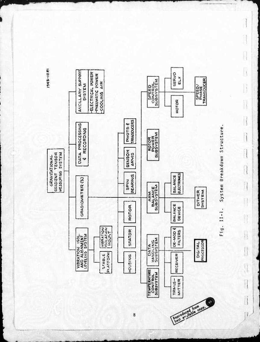
System Breakdown Structure
PAGE
4
8
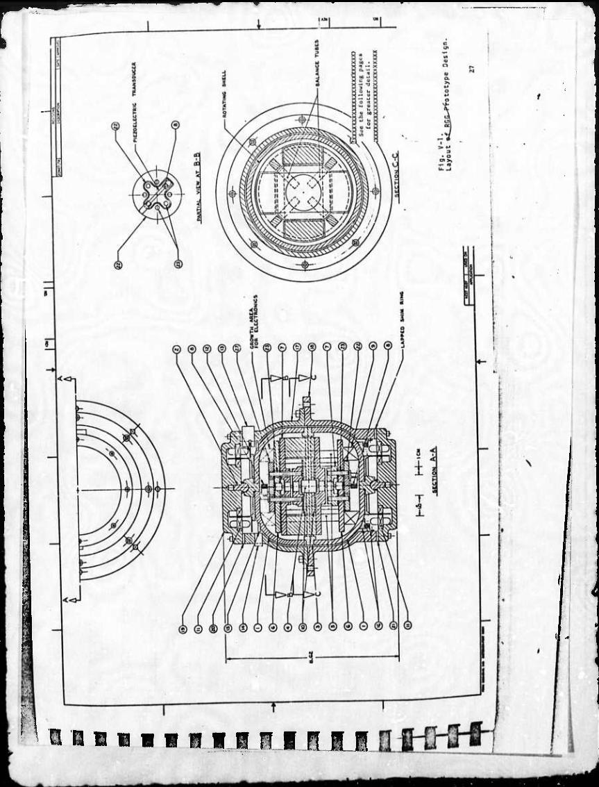
V*l Layout of RGG Prototype Design 27
VIU1 Configuration A 48
VII-2 Configuration B 55
VH-a Configuration B 56
VII-4 Configuration C 57
VIN5 Restraint System Schematic For Tetrahedron Air Pad Sensor Configuration C 58
VIIU1
VIII-2
VIII-3
VIII-4
VIII-5
VIII-6
VIII-7
VIII-8
Acceleration Power Spectra 73
Angular Rate Power Spectrum 74
Acceleration Power Spectra 82
Angular Rate Power Spectrum 83
Six-Element Axisymmetric Linkage Air Column Vibration Isolation Mount 86
Hipernas IIB IRU Specification
Three-rAxis Air Bearing Stabilizer Platform
89
99
Estimated Platform Angular Rate Response to Normalized Torque Disturbance 119
?
IX-1
IX-2
Equivalent Block Diagram of Signal Process
Equivalent Circuit of Signal Sensing and Transducing Process
128
133
ix
• ^^
■1
IX-3 Standard "Deviation Gross Gradient Thermal Noise (9^) Versus Effective Q . .^ 133
IX-4 An Assumed Probability Density Function .... 145
XII-1 Spin Bearing Final Design Gross- Sectional View 197
XIII-1 Solid Bar Structure of Rectangular Cross Section 202
XIII-2 Arm Configuration A 202
XIII-3 Arm Configuration B 203
XIII-4 Arm Configuration - Interleaved 204
XIII-5 Arm Inertia Parameter Versus Width to Radius Ratio 206
XIII-6 Arm Mass With Added Cylindrical Sector Portion 208
XIII-7 Prototype RGG Isoelastic Arm Design 211
XIV-1 RGG Sensor-Transducer Equivalent Circuit 222
XIV-2 Sensor Computer Program 226
XIV-3 Voltage and Phase of Sensor- Transducer Output Voltage 227
XIV-4 Axis Definition for Piezoelectric Ceramics 230
XIV-5 Piezoelectric Bender Transducer 233
XIV-6 Moment and Shear Diagram for One Type of Transducer Loading 235
XIV-7 Moment and Shear Diagram for Second Type of Transducer Loading 237
XIV-8 Equivalent Circuits for Piezoelectric Bender Transducers With Interrelating Equations 240
'
^«■M

I
XIV-9 RGG Sensor Equivalent Circuit 243
XIV-10 Piezoelectric Transducer Computations 247
XIV-11 Piezoelectric Bender Transducer, Series Polarized 248
XIV-12 Computer Program to Evaluate RGG Sensor Temperature Sensitivity 258
XV-1 Rotor Power Subsystem 274
XVI-1 Functional Block Diagram of Servo 277
XVI-2 Speed Control Servo Gain Versus Phase 279
XVI-3 Speed Control Servo Error Response 280
XVI-4 Encoder Disk 289
XVII-1 Remote Arm Balance Subsystem 292
XVII-2 Mass Balance Device 295
XVII-3 Mass Balance Device Mounting 296
XVII-4 Test Signal Generator, Schematic and Waveforms 302
XVIII-1 Thermal Model 304
XVIII-2 Hughes TAP-3 Thermal ANalysis Program 306
XVIII-3 Node 12 Temperature Curve 309
XVIII-4 Node 12 Temperature Curve Without Boundary Temperature Fluctuation 310
XVIII-5 Lower Heater Power Curve With Lower Control Temperature 311
XVIII-6 Oil Film Temperature 312
XVIII-7 Plot of Control Temperature During 10th Operation Hour 314
xi
• -- ' mm—m mm

XIX-1 Signal Readout Subsystem Schematic Diagram 318
XIX-2 Full Scale Mockup of Rotor Mounted Electronics 320
XXI-1 Encoder Disk 325
XXI-2 AM to FM and Signal Counter Switching 326
XXI-3 Minicomputer and I/O For RGG Prototype Design 330
XXIV-1 Sensor Model -Axial Acceleration Effect . . • • 345
11
[I
I
!
I n
xii
I
- ^mt
I I )
]
]
1 1
I I
g
XX
A o A
A.
B
B yy
BN
c
c =
cm
C
C zz
d
dem
D
EU
o
e, Ae
E
f
GLOSSARY OF TERMS
/ 2 -., 2 ,2 acceleration; meters/sec , ft/sec , cm/sec
gravitational acceleration at the surface of the earth
moment of inertia of a body about the x axis
constant (s); ampere; compliance
Angstrom unit = 10 cm
generalized second rank tensor
compliance
moment of inertia of a body about the y axis
noise bandwidth
capacitance, farad
Viscous damping, dyne cm/rad/sec; or compliance l/K of a mechanical system
= centimeters
= c impliance
= moment of inertia of a body about the z axis
= diameter; dynes force; pendulosity distance
= dyne centimeter
= viscous damping
= Eötvos Unit = 10"9 sec" = lO-9 (ft/sec )/ft
= 10'9 gal/cm a 10"1 g's/cm
= temperature coefficient of modulus of elasticity
= mass center eccentricity
= Young's modulus of elasticity
= force; dyne; newton (10 dynes = 1 newton); pounds; frequency
ft = foot
xm

GLOSSARY
F - force; a parameter in surface tension equations; farad
g = earth's gravity
g = 32, 1724 ft/sec2
= 980. 616 cm/sec2
■ 10 milligals
gal = (Galileo) unit of acceleration = 1 cm/sec
gm = grams
G = Newtonian gravitational constant
= 6. 67 x 10 m /kg sec
= 6. 67 x 10" cm /gm sec
31.4 x 10"9 ft4/lb-sec
G = shear modulus
GG = gravity gradient
G.. = gravity plus inertial gradient tensor
hr = hours
Hz = Hertz (2u radians/sec)
H = transrrittance function; angular momentum; inductance in henry; transfer function
h = Planck's constant, mass unbalance distance
I = moment of inertia
IN = noise current
I = in-phase subscript
j = imaginary operator
J = polar moment of inertia; joule
K = degrees Kelvin
k - Boltzmann Constant = 1. 38062 x 10' joule/ K
= I. 38062 x 10"16 ergs/0K
kT 290OK kT170C 4 x 10 14 A 1^-21 . , ergs = 4 x 10 joules
1
I]
I
i VI
1
n
XIV
riM*

!
I 1
r
D i
0
GLOSS A.RV
kg = kilogram
K,k = constant; or spring stiffness; or torsional stiffness
lb = unit of force
£ - length; or separation between masses
L = torque
M or m = mass or meters
m = meter 7 A 23
= mass of the earth = 5.975 x 10 kg, 4.08 x 10 slugs
-3 -3,2 = milligal = 10 gal = 10 cm/sec
= newton; piezoelectric transducer coefficient
= power
= noise power
= signal power
= pendulosity
-12 = picofarads = 10 farads
= dm = pendulosity
= quality factor of a tuned system
Q l^n _ N/IK = ^ = J- = f = 2* times peak Q " D D 2T 2t, 6
energy stored in sensor/(energy dissipated per cycle)
Q = quadrature pha^e subscript
R or r = radius 7
R = Radius of the earth (mean) = 2.09 x 10 ft
RGG = Rotating Gravity Gradiometer
rad = radian
M e
mgal
N
P
PN
PS
r pF
p
Q
XV
MM
- ^M ■te^i Mmm
GLOSSARY
R B
S =
s =
S..
t =
T =
radius of sensor arm
radius of gyration
Laplace transform differential operator, power spectral density
second
rotation matrix
time in seconds; ti» tj""*! = tirne index Points or
intervals
temperature, 0C, 0K or 0F, torque
T s = time of signal
T o
= time ol absence of signal
T ave = averaging time
T. int = integration time
V = volts, /elocity, volume
w = watt
Z,x, y, 9. = used to designate coordinate systems
p
r
GREEK CHARACTERS
= angle, angular acceleration; thermal coefficient of expansion; generalized mode coordinate.
= angle, angular rate, sum-mode resonant frequency
GM . . = —5- in general R3
= gradient error
3GM eq
= equivalent gradient
il
!
I
1
1 1 fl
1
1
!
n 1
"i
1 1
XVI
■i HMiiMnirt

1 - GLOSSARY
1
r.. ii
I
1
1 1 I I I
L
4>
*
e
®
T =
\ =
U) =
I =
H =
Y =
'a " 6 =
P =
P =
n =
o =
A =
= gravitational force gradient
B - A = inertia efficiency ratio r-
zz
frequency; Poisson's ratio
gravitational potential; phase angle
rotation matrix; inertial tensor
angle; radians or degrees
rotation matrix
time constant
wavelength
angle, compliance tenspr
rotation matrix
angular rate or natural frequency
j .. actual damping damping ratio = —rr-—7—3—r . ° r critical damping
micro; magnetic permeability
microfarads = 10" farads
surface tension, cynes/cm, eccentricity ratio
anomalous gradient tensor
Af/fo, ratio of frequency change to resonant frequency; differential angle between sensor arms
density
transport angular rate
Earth's angular rate; natural frequency; ohms
angle, radians or degrees
increment or difference
xvu
MM ^^ m^m^

f
1 GLOSSARY
1 6 = angle
t = gyro drift rate, bearing anisoelasticity
a = standard deviation
MATHEMATICAL SYMBOLS
= equal to A = equal to by definition
= identically equal to
s? approximately equal to
V del or nabla, differential vector operator
PREFIXES
The names of multiples and submultiples of SI Units may be formed by application of the prefixes:
Factor by which unit
is multiplied
10
109
1C6
103
102
10
10"
10"
10"
10"
10"
10'
10
10
12
Prefix
12
-15
-18
tera
giga
mega
kilo
hecto
deka
deci
centi
milli
micro
nano
pico
femto
atto
xvui
Symbol
T
G
M
k
h
da
d
c
m
V-
n
P
f
'1 ]
1
i I
1 '!
D
il
i
B
1
fl
8
^mk

GLOSSARY
PIEZOELECTRIC SYMBOLS
(See Section XIV. )
xix
^mmmmä

I ]
1
I 1 1 I 1 I
I
I I 1 I 1 "1
ABSTRACT
This report covers the technical studies accomplished during
the second six months of this contract to design and develop a proto-
type moving base gravity gradiometer with a sent ivity of better than
1 EU (10'9 sec'2) for a 10 se: integration time. Since the end of this
second report period coincided with the end of the first phase of the
contract, this report is a complete summary of the Phase I design and
analysis work. The report is self-contained in that all material perti-
nent to the analytical and design phase is contained herein with the
exception of references to certain specific sections in the previous Semi-
annual Technical Report (August 1972). The selected rotating gravity gradiometer (RGG) baseline design
2 has an arm length and inertia of 12 cm and 35, 600 gm-cm , and an
overall size and weight of 22 cm by 16 cm diameter, and 9.6 kg. The
sensor spin speed is 1050 rpm (17.5 rps), which is compatible with
the sensor resonant frequency of 35 Hz with a Q of 300. These param-
eters, in turn, determine the sensor time constant to be 2.71 sec;
the remainder of the system integration time (7.29 sec) is determined
by the data processing filtering. In the fully integrated RGG prototype design, we have chosen:
hydrodynamic oil spin bearings; asynchronous drag cup motor drive
with photoelectric position and tachometer speed pickoffs; mechanically
isolated piezoelectric transducer; similarly shaped isoelastic inter-
leaved double-strut sensing arms; electrolytic fine balance adjustment;
multiple torsion bar supports formed from a single rod; internal AM-FM
conversion with external power supply; air core transformer data feed-
through; external FM-digital conversion; digital plus analog data reduc-
tion; and solid mounting oi ^he sensor case to the stable element of the
angular isolation platform. In addition to the gradiometer design studies, th.j report con-
tains specifications for a vibration isolation, alignment and leveling
system (VIALS) for support of the gradiometers during use. For the
xxi
Preceding page blank
^tm ^mm*

11
vehicle and mission we assumed a C-135 carrying out an airborne
gravity survey. The components of a VIALS that would meet the
system performance specifications arc shown to be state-of-the-art
components. An extensive error analysis was carried out on the various
error terms introduced by the assumed environment, the VIALS, and
the gradiometer itself. The estimated errors from all sources are
shown to be less than 0.65 EU for a 1Ü second integration time, which
is well within the design goal. We can report achievement of our goals for this study phase.
The sensor design is complete, and wc are proceeding into the engineer
ing phase where detailed drawings will be prepared prior to faorication
and laboratory test of the first prototype.
I
[I
i
i
i
1
ö
;
1.1
xxu
p
MM ■^

I I I SECTION I
INTRODUCTION
r. I i
i i:
i
This report presents the culmination of the Phase I work carried
out under Contract F I9628-72-C-0222 during the period from 1 Febru-
ary 1972 through 19 January 1973.
The reader Vw * note that Sections IV, V, and VI summarize the
configuration selection rationale, the sensor design, and the error
analyses. The summaries ure intended to provide an overview of the
accomplishments without detailed elaboration or references to other
material.
The Semiannual Technical Report No. 1, dated August 1972, is
included by reference throughout this document to avoid duplication of
previous efforts and to reduce the bulk and cost of this report. Thus,
these two reports are complementary and are intended not only to meet
the contractual requirements but to serve as useful, working documents.
7 he philosophy of a two-phase program, i. e. , study followed by
a review and then hardware, generally proves to be very beneficial
when the state of the art is being advanced. The work under this con-
tract has reaffirmed this desirability. Phase I has provided the
answers to the many tradeoff questions involved in the complex task of
designing a new sensor which incorporates the extraordinary capabilities
that a moving base gravity gradiometer must possess.
The efforts of this past year have provided visibility in pre-
viously unexplored areas. Many problems were uncovered during the
early months, but solutions were found. New problem discovery has
virtually disappeared in recent months, which attests to the progress
C ..A«», ««rffclJ......»^.. '-.t«t^»J •■.»-. ..„„■, .*

SECTION I
i
i
i'l
i
that has been made and the present status of the development. Of
course, analyses and studies cannot provide all the answers; any prac-
tical program must leave the paper phases at an appropriate time and
enter a hardware pha^e. Only then can an unequivocable statement be
made that all problems have been discovered and solutions found.
We can report achievement of our goals for this study phase.
The sensor design is complete, and we are ready to proceed into the
engineering phase where detailed drawings will be prepared prioT to
fabrication and laboratory test of the first prototype.
We have met the Statement of Work error-sensitivity design
goals. The resulting sensor is a sophisticated, logical design based
upon: (1) a great deal of prior analytical and experimental work funded
by AFCRL, NASA, and Hughes, and (2) the analytical and design tasks
of this first contractual phase. The design is a feasible concept
requiring available, or readily obtainable machine tools, test equip-
ment, and test facilities for both manufacture and laboratory testing.
We have retained most of our original sensor concepts, thereby
building upon an already proven base of technology. We have utilized
the services of specialists in certain relatively narrow fields where it
was not cost effective for Hughes to attain new levels of knowledge.
This study phase has reaffirmed the importance of designing a
sensor within the context of the total, integrated system. A gradiom-
eter design study cannot be carried out in isolation from considerations
of the complete gravity gradient measurement system and its ultimate
application. The application sets the desired sensitivity and time con-
slant (these were predetermined by the contract as 1 EU at 10 sec),
while the using vehicle determines the environmental conditions. How-
ever, the coupling of the sensor design is strongest to the isolation and
stabilization platform, and there are many tradeoffs possible between
the sensor and platform parameters. We have taken these tradeoffs
into consideration during this design phase and discuss them further in
Sections VII and VIII.
\
i
0 ] 0
^MMMM^M^i

SECTION I
In summary, the system concept described in this report, and
the RGG sensor design, depicted in Fig. I-1 and 1-2, are fully justi-
fiable. We are confident that Phase I results reflect very well upon a
broad foundation of knowledge and warrant immediate continuation into
the hardware phases of this program to construct the first prototype
moving base gravity gradiometer.
Figure I-1. next page, is 76% of full-scale cross
sectional drawing. The weight is calculated to be
9.6 kg («21 lb).
*«■*

2075-55
Fig. 1-1 Rotating Gravity Gradiometer Cross-Section View (76% of Full Scale).
1 i
n
MM ^mk

I [ I
SECTION I
D
\
© © © © © © © © © © ©
© © © © © © © © © ©
ROTATING GRAVITY GRADIOMETER COMPONENT IDENTIFICATION
Rotor
Spin bearings
Circular central plate of rotor
Pivot assembly
Brace posts (8 total)
End plates
Central assembly and sensor arms
Piezoelectric transducers
Rotor electronics
Mass balance adjusting devices
Motor /tachometer
Position encoder disk
Light source and photo cell
Second light source
Photocells (2 ea. )
FM transmitter output transformer
Stator
Mounting bosses
Motor end cup
Insulator
Lapped shim
Transducer concentric mounting plates
Transducer assembly mounting posts
Electronic growth area
•V n».


I I I 1 r
r.
SECTION II
SENSOR DESIGN INTEGRATION
A moving base rotating gravity gradiometer measurement
system consists of many subsystems; one of these is the Rotating
Gravity Gradiometer (RGG), which itself has many subcomponents
(see Fig. II-l). All of these subsystems and their interactions must
be considered in the design integration task throughout the design
phases. Hughes' 8 years of RGG design and test experience has
established a number of viable concepts for each of the subcomponents
of the RGG. Specific examples of the alternate concepts for some of
the major subsystems in the gradiometer are shown in Table II-l.
All of these alternate concepts were considered many times during
this program.
Before a sensor baseline design could be evaluated, a set of
basic parameters nad to be selected. These basic parameters are:
desired system sensitivity and integration time; size and weight (arm
inertia); sensor resonant frequency and damping ratio; resonant
frequencies and damping ratios of the other major mechanical com-
ponents (support pivots, brackets, and arms); and coupling ratio of
the transducer.
The system sensitivity and integration time were set by the Q 2 contract requirements: 1 EU (10"' sec ) at 10 sec (la). With these
fixed, the remainder of the basic parameters were then determined
(with some tradeoff possible between some of the parameters). The
tradeoffs and selection of the basic parameters were made early in the
program and are given in detail in the Semiannual Technical Report
No. 1 (Section III-C).
During the initial phases of the program, various combinations
of the alternate concepts (Table II-l) were combined into a series
of baseline sensor designs with each design carried out in sufficient
detail to allow the complete sensor to be evaluated.
• - ■
I J
!
ir ? -1 o in < iß H z V W) o in > <=H b>
5 h 15
> 7 DC g 10 Q o 'X < ir UJ o 2
H K (V O III a
si
2 8
10
a <
Jß V- 5 J VJ s8 u 111
ü -J <J UJ
_i_ 1 '
«J
iw in 5 uJ o ^ a r^0
a uj <a
U^ o
/-» (/> v^
a ui i-
s o Q < ct (5
22 OOj-
Jt-S 55^ Ozi" ^^^
2z«n 9§o
0D2>
s
ui
o| - s a £
V!)
2? 9; < (0 UJ
O h 0 a
O
< 1-
2 IT) -I o z
QJ t.
3 4J o 3 t-
■M
2 O
s- co
E <u
to
i
i 1 I
D1
n
^■^i

—,^:
SECTION II
TABLE II-1
Viable Alternate Design Approaches foi- RGG Subsystems
Subsystem
Spin bearing
Sensor arms
Pivots
Transducers
Speed control
Data handling
Housing
Arm balancing
Alternate Concept
Magnetic Oil - hydrodynamic and hydrostatic Air - hydrostatic and squeeze film
Single strut Interleaved double strut
similar shape different shape
Torsinnal - single and double ended
Longitudinal flex leaf (reel) Transverse flex leaf (Bendix)
Capacitive Piezoelectric Optical Magnetostrictive Magnetic flux Mutual inductance
Synchronous Asynchronous - ac and dc Photoelectric, magnetic or mutual
inductance pickoff
Analog Digital FM PCM Combinations of above
Hard mounted Floated - oil
air - pressurized, squeeze film
springs various combinations of above
Piezoelectric Mechanical Sputtering Electrolytic
T874
«MM

SECTION n
For each of these baseline sensor designs, we studied the
effect of the known error excitation sources acting on the sensor
error sensitivity estimated for the particular baseline design. (See
Tables II-2 and 11-^; they are condensed from pages 11 to 17 in the
Semiannual Technical Report No. 1. These show, in more detail, the
many factors involved in the evaluation of a sensor design). From this
serlss of evaluatioi studies, we have chosen a sensor design.
The selected RGG baseline design has an arm size and inertia
of 12 cm long and 35, 600 gm-cm , and an overall size and weight of
16 cm by 22 cm, and 9. 6 kg. (This size and weight will be approxi-
mately the same for all gradiometers with a 1 EU at 1 3 sec sensitivity,
since the thermal noise contribution of the sensor alone becomes larger
than the required sensitivity for smaller sensors. ) The sensor spin
speed is 1050 rpm (17. 5 rps), which is compatible with the sensor
reaonant frequency of 35 Hz with a Q of 300. These parameters, in
turn, determine the sensor time constant to b^ 2.71 sec; the remainder
of the system integration time (7. 29 sec) is determined by the data processing filtering.
In the fully integrated RGG prototype design, we have chosen:
hydrodynamic oil spin bearings; asynchronous drag cup motor drive
with photoelectric position and tachometer speed pickoffs; mechanically
isolated piezoelectric transducer; similarly shaped isoelastic inter-
leaved double-3trut sensing arms; electrolytic fine balance adjustment;
multiple torsion bar supports formed from a single rod; internal
AM-FM conversion with external power supply; air core transformer
data feedthrough- external FM-digital conversion; digital plus analog
data reduction; and solid mounting of the sensor case to the stable
element of the angular isolation platform.
This last feature deserves comment as it illustrates the
fact that a sensor design cannot be isolated from the design of a com-
plete system. Our studies showed that ths sensor sensitivity to
angular rate jitter and alignment errors is the same for all gradiometers,
and that all gradiometers with the same sensitivity will have similar size and weight. fj
10 • j
i
i
(
1
1
I
I
n f]
MM ^mä~m

I I 1
SECTION II
TABLE II-2
Error Excitation Sources
(1) Tranalational Acceleration
(2) Angular Rates and Accelerations
(3) Temperature — (Nominal operating temperature results in thermal noise effects)
(4) Temperature Variation
(5) Ambient Pressure Variations
(6) Ambient Humidity Variations
(7) Magnetic Fields
(8) Electric Fields
(9) Acoustic Fields
(10) Angular Orientation
(11) Mass Proximity Gravity Gradients (including earth)
(12) Prime Power Variations
(13) Time Standard Variations
(14) Component Inherent Characteristics
(15) Material Stability - This - eludes stability of dimensional properties as well as other param- eter changes (e.g., transistor ß's, Youngs mod- ulus, damping coefficient, etc.) resulting from creep, aging, crystal growth, temperature cycling, etc.
T875 • ^
11
«MM M*

SECTION II
TABLE II-3
Error Mechanisms
(1) Translational Acceleration Sensitfvity
(2) Angular Acceleration Sensitivity
(3) Thermal Noise Generation— (Sensitivity to nominal operating temperature)
(4) Temperature Sensitivity— (Sensitivity to vari- ations in operating temperature)
(5) Ambient Pressure Sensitivity
(6) Humidity Sensitivity
(7) Electromagnetic Sensitivity
(8) Electrostatic Sensitivity
(9) Acoustic Sensitivity
(10) Angular Orientation Error Sensitivity
Sensor
VIALS
(11) Gravity Gradient Sensitivity
(12) Prime Power Sensitivity
(13) Time Standard Sensitivity
(14) Component Inherent Characteristics
(15) Material Instability Sensitivity
T876
I
I
12
I H
I R
^^mm ^MrtM^Bt

"■ ^ w*
1 [ r
i
o i
i
i
i
i i
SECTION II
The sensitivity to angular rate jitter and alignment errors
produces a conflicting set of requirements that cannot be met by a
simple flotation system for a gradiometer sensor. If a gradiometer
is to be floated to isolate it from angular rate jitter, it would require a
servo system to maintain the orientation of the sensitive axis of the
sensor with respect to the platform coordinates. If we use a simple
case-oriented servo system that is tight enough to reduce the error
contribution from the coupling of the error in angular orientation to the
background bias of the earth's field, then the servo is so tight that it
will transmit angular rate jitter. Thus, either a floated gradiometer
with a complex servo system or a platform with better bearings or an
angular rate jitter measurement and compensation system is indicated.
The size and weight of a three-axis gravity gradiometer system,
along with the system sensitivity to angular alignment errors, pro-
duce a conflicting set of requirements for the stabiliaation platform.
Available stable platforms with the required angular orientation capa-
bility do not have a payload capability to carry one or more gravity
gradiometers in addition to their own inertial instruments. Therefore,
a new stable platform capable of carrying the weight is required. It must
also possess the desired characteristics of presently available inertial
navigation systems. Fortunately, a new stable platform can be made
easily with bearings providing the required angular rate steadiness,
thus allowing the gradiometer to be hard mounted directly to the stable
element. The design and manufacture of such a stable platform with
the required orientation accuracy, payload capacity, and a high level
of angular rate steadiness is within the state of the art and is a rela-
tively straightforward engineering task.
The above discussicn is but z brief overview. The details of
the design features of the fully integrated RGG prototype design are
covered in Sections IV, V, and VI of this report. Other sections of
this report and the Semiannual Technical Report No. 1 treat each
aspect of the design in detail.
13
tt^^tamm^^tmi ^mm^ttak

SECTION II
The desicjn integration tasks are not completed. They will
continue into Phase II of this program as long as the fine-grained
details of the manufacturing and assembly processes are being exam-
ined and remain open for refinement.
i
I
I
i
1
14
1 T
[
[
[ I r
SECTION III
STATEMENT OF WORK COMPLIANCE
This section reviews the work that has been done during Phase I
of this contract and demonstrates that the technical requirements of
Section F, Description/Specifications, of the Statement of Work have
been completed. Each line item of Section F is reproduced for con-
venience. Following each line item and sub-line item is a brief discus-
sion which demonstrates that the requirements of the line item have been
met. In many cases, specific sections of the Semiannual Technical
Report No. 1 and of this report are referenced to demonstrate specific
compliance.
A. LINE ITEM 0001
Design a moving base gravity gradiometer capable of measuring
directly the horizontal and vertical gradients of gravity and serve as the
basic sensor(s) for the following applications: marine, airborne and
satellite gravimetry: determination and recording of the variation of
the deflection of the vertical along the path of a vessel; augmenting on
real time basis an inertial navigation system of a submarine, ship or
aircraft; and in static mode of operation for mass detection.
Discussion
The one rotating gravity gradiometer sensor (RGG) design
summarized in Sections IV, V, VI, und VII will measure directly the
horizontal or vertical gravity gradient tensor elements, The tensor
elements measured will depend on the orientation of the spin axis.
Three sensors are required to measure all of the unrelated gravity
gradient tensor components. The same sensor and electronics can be
used for marine and airborne gravimetry. The same sensor
15
itaM
■MM

SECTION III
(three required) and electronics, along with other necessary computers,
stable platforms, and recorders can be used to determine and record
the variation of the deflection of the vertical along the path of a vessel
and to augment on real-time basis an inertial navigation system of a
submarine, ship, or aircraft. The RGG sensor can be used in the
static mode for mass detection.
Satellite gravimetry would require a sensor of greater sensitivity
than that specified oy this Statement of Work. A preliminary design has
been completed by Hughes for NASA. The design is based upon the same
basic RGG concept of a torsionally resonant pair of rotating arms, but
which are much larger in their dimensions. It also differs because a
spinning, orbiting satellite vehicle is assumed, which eliminates the
need for the spin bearings and the isolation subsystems.
In summary, the one RGG that has been designed meets all of
the requirements of Line Item 0001.
1
B. SUB-LINE ITEM 0001AA
Perform analytical studies for the determination of design
parameters and configuration of a gradiometer capable of measuring
any horizontal and vertical gravity gradient components to a one stan-
dard deviation accuracy of one EU (EU = Eotvos Unit = 10"^ sec"2) or
better for a 10 second integration time. If a design requires different
sensors for the measurement of horizontal and vertical components
both types of sensors will be included.
Discussion
Analytical studies of several gradiometer configurations havo
been made. These are reviewed and summarized in Section VII of this
report. Extensive error analyses hive been made; some of these are
given in the Semiannual Technical Report No. 1, and others are shown
in Section IX of this report. In addition to these analyses, the errors n l
16 • )
— ^■■fc

r r r. r.
r r D
i:
SECTION III
due to each component or subsystem are evaluated as part of the
subsystem design, and this material appears in the appropriate sec-
tions. Section VI provides an error analysis summary which demon-
strates that the Prototype RGG Design used in a three-sensor system
has a 1-sigma error of less than 1 EU at the gravity gradient tensor
element. The one sensor design can be used in any orientation.
The requirements of Sub-Line Item 0001AA have been fulfilled.
C. SUB-LINE ITEM 0001AB
Conduct laboratory experiments with existing instruments (if
any) to complement and substantiate the results of analytical studies.
Discussion
Laboratory experiments were conducted on an existing RGG.
Specific acceleration sensitivities were measured and studied. These
are discussed in Section XXIV of this report. The prototype RGG
design avoids the problems encountered in the older design. Sub-Line
Item 0001AB requirement has been satisfied.
D. SUB-LINE ITEM 0001AC
Study the stabilization and motion isolation requirements for the
recommended gradiometer design considering the most critical applica-
tion. Determine required platform and isolation systems parameters.
Demonstrate in form of studies that any component of the motion isola-
tion system, external to the basic gradiometer, required for the support
and isolation of the sensor is within the current state-of-the-art
technology.
I
17
.«•Ma **m

SECTION III
Discussion
This requirement has been studied since the receipt of the RFP.
The final summary is in Section VIII cf this report. The airborne
environment is considered to be the worst case, and all components
are within the current state of the art.
Sub-Line Item 0001AC requirements have been fulfilled.
E. SUB-LINE ITEM 0001AD
Determine design parameters and final configuration of the
proposed gravity gradient sensor(s).
Discussion
The design parameters of the RGG Prototype Design are tab-
ulated in Section V of this report. The final configuration is also shown
in that section. Sub-Line Item 0001AD requirements have been met.
F. SUB-LINE ITEM 0001AE
Data in accordance with Contract Data Requirements List (CDRL)
DD Form 1423, Exhibit "A" (Revised) dated 72JAN19.
Discussion
Data has been provided in accordance with this list. This
requirement has been met.
18 1
.^

I T 1 1 1 1 1 1 1
SECTION IV
RGG CONFIGURATION SELECTION SUMMARY
This section is a summary of Section VII which describes our
rationale which led to the selection of the prototype configurations of
both the RGG sensor and its required motion isolation system.
A large portion of this study effort has been devoted to selecting
the most cost-effective configuration of the required moving base
gravity gradient measurement system. Because of the inherent sensi-
tivities of any realizable gravity gradient sensor to translational and
rotational motions induced by the carrying vehicle, design of the
prototype RGG sensor is heavily linked with the characteristics of the
vibration isolation, alignment, and leveling system (VIALS) used to
support a three-sensor group. Although design of the VIALS has not
been required, study of its performance requirements and charac-
teristics, aswellas demonstration of its state-of-the-art feasibility,
has been a contractual requirement of this study (see Section VIII).
Because of the inherent rotational field error sensitivity of
any gravity gradiometer.to angular rates of its measurement refer-
ence frame, primary consideration was given to selecting an RGG
VIALS system combination which leads to the most cost-effective
solution of this probleI.,. Indications from earlier Hughes studies,
reconfirmed during this study, showed that stabilized platforms,
utilizing conventional ball-type gimbal bearings, do not provide the
required angular rate steadiness. Thus, our original design goal was
to seek a solution to this problem by incorporating an angular rate
isolation capability in the RGG sensor.
During studies conducted in preparation for our proposal for
this study contract, many alternative sensor configurations were con-
sidered that could provide this angular rate isolation. A neutrally
buoyant rotating sphere configuration appeared the most promising
19

SECTION IV
and was the recommended baseline configuration in our September 1971
proposal, although its practical design details had not been studied
in depth. Several of the other alternative configurations still remained
practical and feasible. It was realized that more detailed studies
would have to be carried out in order to learn the pitfalls and advan-
tages of each. After receipt of the contract, preliminary design
studies of the proposed baseline and the most promising alternatives
were undertaken. The four configurations studied are briefly
described below.
A. CONFIGURATION A - NEUTRALLY BUOYANT ROTATING SPHERE
The basic RGG arm pair is mounted in a spherical float
centered in a spherical, fluid-filled rotor. The rotor is spun on its
spin bearings at the required sensor spin frequency. The transverse-
to-polar moment of inertia ratio of the float is designed such that
the preferred axis of spin of the float results in the sensitive axis of
the sensor arm pair maintaining its average alignment coincident
with the spin bearing axis. Any angular vibrations of the spin bearin|
stator are isolated from the float via the small viscous coupling
between the float and the rotor.
I
B. CONFIGURATION B - TWO -AXIS AIR BEARING GIMBAL
The sensor arm pair is mounted directly to the rotor and
rotates in the spin bearings. The angular isolation is provided by
supporting the stator by an air bearing, two-axis ring gimbal.
similar to the suspension of a 2 degree-of-freedom gyro.
20
•«■MM mtm *Mü

i
SECTION IV
C. CONFIGURATION C - RESTRAINED TETRAHEDRON AIR PADS
The sensor arm pair, rotor, and spin bearings are identical
to that of Configuration B. The sensor stator is spherical and the
angular isolation is provided by supporting the spherical stator by
four spherical-segment hydrostatic air bearing thrust pads located at
the outer surface of the stator. Each pad is placed at the corner of
a circumscribed equilateral tetrahedron which provides an isoelastic
support for the stator. The suspension is constrained to have only
2 rotational degrees-of-freedom by a system of taut restraint wires
connected from the stator to the housing.
D. CONFIGURATION D - DIRECT MOUNTED SENSOR
The sensor arm pair, rotor, and spin bearings are identical
to Configurations B and C. The sensor stator is mounted directly
to the stable element of the VIALS stable platform. The required RGG
sensor angular rate isolation is provided by the stable platform via
substitution of hydrostatic air bearings for the conventional ball-type gimbal bearings.
E. TRADEOFF COMPARISONS
Although the neutrally buoyant rotating sphere intuitively
appeared the simplest and most straightforward of the configurations
which incorporate self-contained angd ir isolation, it subsequently
was proven to be the least attractive. Computer simulation results
showed its angular isolation to be marginally adequate and that it
would require very fine adjustment of the float's polar-to-transverse
inertia ratio. These computer results were questioned because
previous experience in fluid-rotor gyroscope development has
indicated large discrepancies between the analytically predicted and
21
M^a^i

SECTION IV
experimentally determined damping coefficient. Also, apparent
disturbance torques were observed, although their cause has not been
understood. Other practical design and assembly problems were
found which are more numerous and their solutions more compiex,
technically questionable, and costly than any of the other configurations.
Initially, it was thought that both configurations B and C could
be mechanized using only passive, mechanical spring and damper
elements to provide the necessary spin-axis alignment and stabilization.
Dynamic analysis, however, showed that this was not the case
and that an active servo feedback system employing torquers and angle
transducers on the two axes would be required. The conflicting
requirements of providing a low-bandwidth servo response to external
angular rates, but high-bandwidth response to torque disturbancos,
implied that a multiple-loop servo design would be required. The
only conceptually feasible method of implementing this multiple-loop
design would be to employ two single-degree-of-freedom integrating
gyros, or their equivalent, in the servo design. Aside from the imprac-
tical, complex, and costly servo system required, no other signifi-
cant design or assembly problems were formed for either Configura-
tion B or C. Configuration C is preferred over Configuration B
because of its inherently isoelastic suspension of the rotor and its
somewhat smaller size and weight.
The direct mounted Configuration D sensor is, of course, the
least complex and costly of all the configurations studied. In this
configuration, the stable platform gyros provide the necessary iso-
lation and stabilization for all three RGG's simultaneously, instead
of requiring two additional gyros per RGG as would be necessary for
Configurations B or C.
Considerable effort has been expended to determine the availa-
bility of a stable platform having the required level and azimuth
accuracy and the space and weight carrying capacity for mounting
three RGG sensors. No such platform meeting all of these requirements
■j
I
■I
II
22
- — ^«^

SECTION IV
in one system is known to be operational or under development, thus
it has become obvious that a new platform will be required.
The stable platform long-term level and azimuth accuracy-
requirements are stringent and can only be met by careful design of
the platfoim and use of very high quality, "inertial grade" gyros and
accelerometers. These requirements hold for all of the RGG con-
figurations studied and for any other type of gravity gradiometer as
well. A study has been made to determine the feasibility, practicality,
and costs associated with the additional angular rate steadiness require-
ment imposed cm the stable platform if the direct mounted Configura-
tion D sensor is utilized. Incorporation of hydrostatic air gimbal
bearings in the new platform design would provide the required angu-
lar isolation; it is feasible and within the current state of the art, and
it is not a major cost factor (approximately 5 to 10% of the total plat-
form cost).
F. CONCLUSION
The least complex and most cost-effective solution to the
angular rate isolatijn problem has been sought. Schedule require-
ments and budget limitations precluded selection of a system con-
figuration requiring significant development effort or high technical
risk items. Complexity and technical risk considerations ruled out Con-
figuration A. Configurations B and C require a complex, costly
mechanization using two integrating rate gyros per sensor (a total of
six rate gyros per system in addition to the VIALS stable platform
gyros); B and C are considered impractical.
Configuration D imposes the least technical risk and cost of
development of the RGG sensor itself. The additional angular rate
steadiness requirement imposed on the stable platform does not
23

SECTION IV
represent a significant incremental cost or i technical risk.
Complexity, technical risk, and cost effectiveness of the total opera-
tional system being considered, Huphes selected the direct mounted
configuration to build in Phase II of this contract.
I
1
• 1
I
n
'•I
24 P
-

1
■5^
:
D
i
SECTION V
RGG PROTOTYPE DESIGN SUMMARY
A. GENERAL
This section provides a brief tabulation of the RGG Prototype
Design parameters, provides a sensor layout, and incorporates the
Semiannual Technical Report No. 1 and the original Prototype Moving
Base Gravity Gradiometer proposal as parts of this report. The pur-
pose of this section is to provide a ready reference of important param-
eters. Detailed calculations, tradeoffs and assumptions are given in
the sections relating to each parameter. Table V-1 provides the
parameter summary.
B. RGG DRAWING
A layout of the RGG prototype design is shown in Fig. V-l. The
rotor (1) is generally spherical, but is slightly flattened at the ends to
provide a mount for the spin bearings (2). The main member of the
rotor is the circular central plate (3). The pivot assembly (4) is
fastened in the center of the central plate. Eight brace posts (5), four
on each side, are fastened to the central plate (3), and end plates (6)
are in turn fastened to the brace posts. The outboard end of the pivots
are fastened to the end plates.
This central assembly forms a rigid cage-like structure that
completely supports the arms (7), the pivots, and the transducers (8).
Thus the central rotor structure can be assembled, balanced, and
tested before the rotor end bells (1) are put in place. The rotor elec-
tronics assembly (9) is fastened to the previously mentioned end plates
(6). The sensor arms (7) are interleaved during assembly so that the
arms are identical. The mass balance adjusting devices (10) are
mounted on circular disks and these disks are fastened to the arms
25
- - - i^^i
■^-
;
I '
aHHWiHHIHFÜfüH
«MM *tmM mam

1 SECTION V
1 TABLE V-l
i RGG Prototype Design Parameters 1
1. Sensor Undamped Natural Frequency
W« 220 rad/sec
f 35.014 Hz o
2. Sensor Rotational Speed
u 110 rad/sec s
f s 17.507 Hz
3. System Integration Time, T. 10 sec
T. = T + T i s F
T = sensor time constant = 2C*/W s o 2.73 sec
T = filter time constant = T. - T F i s
7.27 sec
4. Sensor Q with Output Load 320.9
Q Unloaded Sensor 640.9
5. Sensor Arms, each
Material 6061 Al
Mass 1.563 kg
Inertia A 4. 990 x 10" kg m A ?
Inertia B 35.610 x 10" kg m
Inertia C 35.600 x 10"4 kg m2
Inertia Efficiency, n = (B-A)/C 0.861
6. Sensor Arm Torque and Energy 1 1
Gradient input torque = M = r|Cr /2
Peak arm torque = rjCQF /2
1. 533 x lO^Nm/EU
4. 599 x 10"10Nm/EU
7. Rotor, Including Arms
Material 6061 Al
Mass
Inertia I zz
5.876 kg
203.9 x 10"4 kg m2
-4 2
■ Inertia I =1 xx yy
144 x 10 kg m
Preceding page blank 29

^v
SECTION V
TABLE V-l
RGG Prototype Design Parameters (Continued)
Mass unbalance about spin, allowed
Angular momentum at 1050 rpm
8. Stator
Material
Mass
Inertia I zz Inertia I
I 0. 03 gm cm 6 2 / 22.4 x 10 gm-cm /sec
6061 Al
3.766 kg 2 m 252.6 x 10' kg
289.2 x 10"4 kg
2 m xx yy
9. Transducer
Material PZT-5A
Output capacity, C0 3.491 nF
1. 302 x 106 ohm Output impedance at w - 220
Output load resistor, R 9. 55 M ohm
Output volts, E 95.86 nV/EU
10. Preamplifier and FM Transmitter
Carrier frequency 200 kHz
Average frequency deviation per EU 2. 78 Hz/EU
11. Rotor Power Supply
Input power frequency 500 kHz
Filtered dc output 10.7 V
Output current 16. 0 mA
12. Rotor Logic
States available 8
States used 6
States spares 2
Logical 1, interrupt power supply 0. 1 ms
Logical 0, interrupt power supply 0. 3 ms
1
i
i I
■
!
30
1 0 P /
mm *CM

■^v my
I 1 SECTION V
1
TABLE V-l
RGG Prototype Design Parameters (Continued)
r.
r
r
]
\
i i i
13. Arm Mass Balance and Balance Devices
Balance devices per arm per axis
Range of balance adjustment per arm per axis, Amh
Balance adjustment resolution
Differential arm mass unbalance allowed,
Bias
10 hour variation, 3or
Arm unbalance sum allowed.
Bias
10 hour variation, 3 cr
Balance device balance change speed
14. Arm Anisoelasticity
Percent mismatch allowed
Prime Anisoelastic Coefficient at Tensor Element
Stability of Prime Aniso-Coefficient
Natural Frequencies (Includes pivot spring rates)
Lateral Bending or Longitudinal Mode
Flapping (Axial) Bending Mode
See-Saw (Rocking) Mode
15. Temperature Control
Nominal operating temperature
Temperature variation of arms, pivots, and transducer allowed,
lor over 3 hr
10
±57 x 10" gm cm
±4x10 gm cm
±2x10 gm cm -4
2x10 gm cm
±8x10 gm cm -4 2x10 gm cm
1. 78 x 10"4 gm cm/hr
0. 1%
1800 EU/g'
0.0075 EU/g'
779 Hz
673 Hz
567 Hz
530C
0.00114OC
31
^k^MMMMOBM^flBi

'W*'
SECTION V
TABLE V-l
RGG Prototype Design Parametjrs (Continued)
16. Spin Motor/Tachometer
Type Two-phase, drag cup
Excitation frequency, nominal 140 Hz
7. 68 x 105 dem Stall torque, 2 motors
Stall watts, 2 motors 30.2 W
6. 7 x 10⁴ dem Running torque at 1050 rpm, 1 motor
Running watts at 1050 rpm, 1 motor 9. 94 W
1.29 x 10'2V/rad/sec Tachometer scale factor
17. Spin Bearing
Type Hydrodynamic oil
Form Hemispherical
Running torque at 1050 rpm, 2 bearings
4 5x10 dem
5 x 10⁵ dem Breakaway torque, 2 bearings
Bearing radial clearance 220 fi in.
Bearing stiffness 1.63 x lO5 lb/in.
18. Sensor Pivots, All Pivots Identical
Material
Shear modulus
Beryllium-Copper
4. 5 x lO10 N/m2
Temperature coefficient of shear modulus -330 ppm/ C
Active length, each pivot 0.05563 in.
Active diameter, each pivot , 0.05563 in.
Torsional Spring Rate 12. 5 Nm/rad
19. Digital Computer
Word length 16 bit
Memory 8K of 16 bit
Add or subtract 2. 5 jjisec
Multiply 12 (isec
32
f]
'
'I
0 !
1 i
!
i
11
I 11 ll I i
/
m—m *a

I I 1 I f
r. [
i i i i i i
SECTION V
TABLE V-l
RGG Prototype Design Parameters (Continued)
Divide 15 jisec
Access I/O Channels 10 jisec
20. Frequency Refe rence
Type Quartz Crystal
Make Hewlett-Packard
Model number 10544-A
Frequency 10 MHz
Drift
per day <5 x 10"10 Hz
<1.5 x 10"7 Hz
15 min
per year
Stabilize to 5 x lO"9
as shown. The rotor end bells (1) are sealed to the central plate after
the central assembly is complete. A motor/tachometer (11) is fixed to
the stator and encloses the spin bearings. At one end of the rotor is the
position encoder disk (12) with its associated light source and photo-
cell (13), which is attached to the stator. At this same end of the
stator is another light source (14) that excites two photocells (15) on
the rotor. These two photocells piovide the reference for the sensor
test signal.
At the sensor end opposite that used for the photocells and the
encoder dick is the FM transmitter output transformer (16). This
transformer is made up of two concentric coils, one fixed to the rotor
and one fixed to the stator. The stator (17) is made in two parts and
has mounting bosses (18). Rotor input power is provided by insulating
one motor end cup (19) with insulator (20). The capacitance between
the motor and drag cup and between the two halves of one spin bearing
conducts the electric power to the rotor. End play of the spin bearings
is adjusted by means of the lapped shim (21). The piezoelectric
33

9^^
SECTION V
transducers (8) are mounted on concentric plates» (22). These plate!
are in turn fastened to the sensor arms by means of posts (23).
C. SEMIANNUAL TECHNICAL REPORT NO. 1
n
The Semiannual Technical Report No. 1, Contract
F19628-72-C-D222, Project Code PIF10. August 1972, is considered
to be a part of this Design Evaluation Report when referenced herein. n D. PROTOTYPE MOVING BASE GRAVITY GRADIOMETER
PROPOSAL
les The Prototype Moving Base Gravity Gradiometer, Hughe
Research Laboratories Proposal 71M-1593/C3755, Parts 2 and 3,
Technical Proposal, September 1971, is considered to be a part of
this Design Evaluation Report when referenced herein.
!
11
i
IT n
34
f1
MM ^M riHtil

I I !
I I I I I I I I I
SECTION VI
ERROR ANALYSIS SUMMARY
This section provides a concise summary of all errors of an
operational RGG Prototype Design System. The errors due to a state-
of-the-art navigation and vibration isolation system are shown, as well
as the errors due to the RGG itself. The estimated errors for the sys-
tem as a whole are well below I EU, 1 sigma. The errors for the
RGG sensor are only about one-half EU, 1 sigma. Thus a large safety
factor is available in the sensor design. In paragraph A, each error
term is briefly described so that the terms in the RGG System Error
Summary (Table VI-1) can be easily understood.
A. BRIEF ERROR DESCRIPTIONS
1. Thermal Noise
The main source of thermal noise is associated with the dissi-
pative elements of the signal sensing and transducing process of the
RGG. An additional minor source is associated with the signal proces-
sing electronics. Both noise sources are assumed to have white spec-
tra at their origin, and they enter the RGG signal process in the carrier
domain. The selective RGG filter process passes the thermal noise
power located in narrow frequency bands centered at the positive and
negative tuned frequencies of the carrier filter process, nominally
twice the RGG spin frequency. In this analysis, the noise power is
evaluated for a temperature of 326 K, which corresponds to 127.4 F.
2. Sum Mode Mismatch
The "sum mode mismatch' error mechanism provides an
excitation of the RGG differential mode through RGG rotor spin axis
35
«
^■MÜ mm

ri^^H
SECTION VI
TABLE VI-1
RGG Prototype Design System Error Summary
Gravity Gradient Tensor Element Errors, la
Error Sources *xx 'YY 'zz ''XY 'xz ""YZ
RGG Errors
Thermal noise
Arm mass unbalance
Sum mode mismatch
Scale factor
Phase Errors
Rotational field
Anisoelastic
0.338
0.218
0.093
0.150
0.003
0.027
0.017
0. 338
0.218
0.093
0. 150
0.003
0.027
0.017
0.338
0.218
0.093
0.212
0.003
0.027
0.020
0.358
0.231
0.098
0.045
0.033
0.028
0.014
0.358
0.231
0.098
0.002
0.325
0.028
0.010
0.358
0.231
0.098
0.002
0.325
0.028
0.010
RSS of RGG Errors 0.441 0.441 0.465 0.442 0.547 0.547
VIALS Errors
Arm mass unbalance
Rotational field
Anisoelastic
Platform orientation
0.036
0.086
0.069
0.368
0.036
0.086
0.069
0.36J
0.036
0.086
0.135
0.212
0.038
0.079
0.016
0.352
0.038
0.079
0.011
0.327
0.038
0.079
0.011
0.327
RSS of VIALS Errors 0.386 0.386 0.286 0.377 0.339 0.339
RSS o* RGG and VIALS 0.586 0.586 0.546 C.581 0.643 0.643
I
i
11
I
n
36
11
I /

I I I I r r
r r
i i i i i
i
SECTION VI
accelerations occurring in a narrow frequency band centered at twice
the spin frequency (Zw ). This error sensitivity is proportional to
the difference of the squares of the torsional natural frequencies
defined by each arm polar inertia and its associated torsional elastic
coupling to the rotor case (end pivot). Both deterministic and random
excitation of this error mechanism may occur. Deterministic excita-
tions produce bias errors that may be compensated during RGG calibra-
tion to the extent that these excitations remain stable after calibration.
Changes of the deterministic excitations after calibration produce both
bias and random errors depending on the statistical character of the
changes. All excitations of this error mechanism occur by virtue of
disturbance torques acting on the RGG rotor about its spin axis in a
narrow frequency band centered at twice the spin frequency. Potential
excitation sources are the spin bearing; the spin motor; the speed
control servo; and the vibration isolation, alignment, and leveling
system (VIALS). i
3. Axial Torsional Coupling
This error mechanism is sometimes called "The Yankee
Screwdriver Effect" for obvious reasons. It is characterized by a
coupling between RGG axial translational acceleration and RGG differ-
ential mode excitation in a narrow frequency band centered at twice
the spin frequency. Its potential excitation sources are the spin bear-
ing, the spin motor, and the VIALS. In the RGG prototype design, the
pivots, transducer mount and the transducers have all been designed
to eliminate this effect. The sensitivity is assumed to be negligible.
4. Transducer Axial Acceleration Sensitivity
Axial translational acceleration of the RGG rotor in a narrow
frequency band centered at twice the spin frequency will produce
stresses in the differential mode transducers that may generate error
signals due to differences in the electromechanical characteristics of
37
riM*

SECTION VI
the transducers. The potential excitation sources are the spin bearing,
the spin motor, and the VIALS. It is shown in Section XIV that, to the
first order the transducers are insensitive to axial acceleration.
5. Transducer Transverse Acceleration Sensitivity
Accelerations normal to the RGG spin axis in narrow frequency
bands centered at the spin frequency and its third harmonic will pro-
duce stresses in the differential mode transducers which may generate
error signals due to differences in their electromechrnical character-
istics. The potential excitation sources are the spin bearing, the spin
motor, RGG rotor mass unbalance, and the VIALS. It is shown in
Section XIV that, to the first order, the transducers are insensitive to
transverse acceleration.
6. Differential Arm Mass Unbalance
When the mass centers of the RGG arms do not coincide with
a line parallel to the torsional elastic axis of the arm support struc-
ture, a differential arm mass unbalance condition exists. Case-
referenced accelerations of the RGG rotor normal to its spin axis in
narrow frequency bands centered at the spin frequency and its third
harmonic will act on the differential arm mass unbalance to produce
error signals at twice the spin frequency in the carrier domain. The
potential excitation sources are the spin bearing, the spin motor, the
RGG rotor mass unbalance, and the VIALS.
7. Axial Arm Mass Unbalance
When the mass centers of the RGG arms are separated axially
and in addition are displaced normal to the torsional elastic axis of
the RGG, case-referenced angular accelerations of the RGG rotor
about axes normal to the spin axis in narrow frequency bands centered
at the spin frequency and its third harmonic will produce error signals
38
■
I
0 \]
i
"i
n i n
ii
x
^^ mm m*m

^■^^i
1 I I
-
I i
SECTION VI
at twice the spin frequency in the carrier domain. The potential
excitation sources are the spin bearing, the spin motor, the RGG rotor
mass unbalance, and the VIALS.
8. Cross Anisolelasticity
When the principal transverse elastic axes of the arms are not
exactly normal to the RGG torsional elastic axis, and. in addition, the
principal compliances of each arm are unequal or unequal to each
other, a cross-anisoelastic condition exists. Under these circumstan-
ces, case-referenced accelerations of the RGG rotor normal to the spin
axis in narrow frequency bands centered at the spin frequency and its
third harmonic will produce differential error moments at twice the
spin frequency. The potential excitation sources are the spin bearing,
the spin motor, the RGG rotor mass unbalance, and the VIALS.
9. Prime Anisoelasticity
When the principal transverse compliances of the arms are
unequal, a prime anisoelastic condition is said to exist. Under these
circumstances, the low frequency components of the squares and
products of the RGG case-referenced rotor specific forces normal
to the spin axis will produce error moments in a narrow frequency
band, centered at twice the spin frequency. Potential sources of exci-
tation are the spin bearing, the spin motor, rotor mass unbalance,
and the VIALS. The most significant errors are those involving the
gravitational specific force. It is anticipated that these error terms
will be of sufficient magnitude to require active compensation. After
active compensation, both deterministic and random errors must be
considered. The deterministic errors can be compensated during
RGG initialization to the extent that they remain stable after initializa.
tion. Changes of the deterministic errors after initialization produce
trend effects primarily, e.g., bias changes directly proportional to
altitude. The most significant random errors after the compensation
and initialization processes are due to the random vertical accelera-
tions of the VIALS.
39
^—M

«IIUP"
SECTION VI
10. Rotational Field Errors
The rotational field errors of any gravity gradient instrument
are not the result of an error mechanism within the basic instrument
itself. All gravity gradiometers which are based on mass attraction
phenomena (this includes all presently known instrument types) are in
reality specific-force gradiometers. As a consequence, such instru-
ments sense the specific force gradient of the rotational field of their
measurement frames in addition to that of the mass attraction (gravity)
field. All such instruments must be compensated for the known deter-
ministic rotational field gradients. The errors remaining after com-
pensation are primarily random in nature and the result of the random
angular velocities of the VIALS. Rotational field specific force gradi-
ents that arise from self-excitation of the RGG due to its spin bearing,
spin motor, and rotor mass unbalance are primarily deterministic
and are compensated during the RGG system initialization process.
11 Signal-Dependent Scale Factor and Phase Errors
Within the class of signal-dependent errors are those due to
RGG instrument scale factor, RGG instrument phase, and uncertainty
in orientation and position of the RGG system measurement frame.
The first two error mrchanisms are instrument-related (scale factor
and phase), and the latter two are related to the uncertainty in angular
orientation of the VIALS and the position uncertainty of the navigation
system associated with the RGG measurement system. The initial
scale factor and phase of the RGG measurement system are established
and calibrated during the system initialization process. Changes of
RGG scale factor and phase after calibration are due primarily to
temperature sensitivity and aging of the instrument parameters associ-
ated with the signal sensing and transducing process. In addition,
phase variations associated with the signal modulation and demodulation
i
i
|
i'l i
40
I 0 p /
- '—

I I 1 1 T I r i
i i i i i
SECTION VI
processes contribute to this class of errors. Phase variations
associated with the speed control servo as compensated by the signal
demodulation process are the result of torque disturbances and servo
position measurement noise. There are two classes of phase errors
in the RGG signal process. Phase errors that are the result of speed
control servo torque disturbances, by virtue of the servo design and
the method of signal detection, occur in a narrow low frequency band
centered near a frequency of 0.3 rad/sec (approximately 0.05 Hz).
There is no dc transmission of this class of phase error. The other
class of phase errors is low frequency (below 0. 05 Hz to dc) in charac-
ter. This class is the result of changes in the RGG carrier filter
transfer function after initial alignment and changes in the alignment
of the various mechanical elements associated with the RGG position
measurement for the speed control servo. Potential sources of speed
control servo torque disturbances are the spin bearing, the spin motor,
and the tachometer. Potential sources of the second class of phase
errors are resonant frequency variations of RGG differential mode,
changes in the transducer and electronics, variations in the following
alignments: RGG arms co rotor case, speed control servo position
index disk to rotor case, and speed control servo position pick-off
to stator case, and variations in the position pick-off threshold. Vari-
ations in frequency of the time standard (310 ) produces a negligible
error.
12. Extraneous Fields
A general class of possible errors of an RGG measurement
system may be considered in relation to its sensitivity to various
fields of the external environment. Perhaps the most obvious error
source in this class is the time-varying mass attraction field in the
immediate vicinity of the measurement system due to the presence of
the mass of the carrying vehicle and its payload. Generally speaking.
41

13. Ambient Effects
It is believed that RGG sensititivity to ambient humidity,
ambient pressure, and acoustic pressure will be negligible. Temper-
ature effects and prime power variations are considered in relation
to all previously listed error mechanisms.
42
SECTION VI
the gravity gradient magnitudes associated with various parts of the
vehicle and payload must be examined to determine the necessity of
real-time compensation for this effect. Due to the close proximity
of the stable platform gimbal structure to the RGG instruments, it is
highly probable that a deterministic compensation will be required for
changes in the relative mass distribution of the stable platform.
Most materials suitable for use in the construction of an RGG
are paramagnetic, and magnetic fields can produce error moments
at the even harmonic of the spin frequency. It is believed that all
magnetic fields except that due to the earth can be kept negligibly small
in the vicinity of the RGG. It is planned to determine experimentally
the magnetic field sensitivity of the RGG and to provide sufficient
magnetic shielding, if necessary.
It is believed that excitation of the RGG differential mode by
electrostatic fields will be negligible. Electrostatic charge buildup 1
on the rotor may produce torques on the rotor, but this effect will not
produce a differential moment on the RGG aims.
1
R 0 B
1 II
11 i /
+*^~^mim*ammmtmama

SECTION VII
CONFIGURATION SELECTION RATIONALE
I
A. GENERAL
Selection of the prototype RGG sensor and the prototype vibration
isolation, alignment, and leveling system (VIALS) configuration for an
operational gravity gradient sensing system has been a significant por-
tion of this Phase I study effort. Because of the inherent error sensi-
tivities of any realizable gravity gradient sensor to translatory and
rotational motion induced by the carrying vehicle, design of a prototype
sensor capable of operating in a moving base environment is strongly
linked with the characteristics of the VIALS used to support the sensor.
Although design of the VIALS has not been required, study of its per-
formance requirements and characteristics, as well as demonstration of
its state-of-the-art feasibility, have been a contractual requirement of
this study. This section discusses the design goals and the many trade-
offs considered in selecting the prototype configurations ol both the
Hughes RGG sensor and the VIALS.
B. PERTINENT DESIGN GOALS
The primary consideration in selecting an optimum configura-
tion of both the RGG and the VIALS has been cost and operational effect-
iveness of the total system. The requirement of this study was to
develop a gradiometer which would serve as the basic sensing element
in an operational system that will provide for measurement of all ver-
tical and horizontal gravity gradient components. It requires three
Hughes RGG sensors operating with mutually orthogonal spin-axes to
provide all of these specified components. Hence, this study has been
confined to optimizing a system consisting of a VIALS and three RGG
43
M ^MÜ
nmm
•*»•■
SECTION VII
sensors. The fact that this specific system configuration was optimized
is important. In some potential applications, a single RGG sensor could
provide the necessary measurement, hence the angular isolation portion
of the system might take a considerably different form.
It had become apparent that one of the very dominant problems
in developing an operational moving base gradiometer was to provide a
feasible and practical solution to the inherent rotational field error
sensitivity of a gradiometer. Hence, a primary design goal was to
develop a system that would solve this problem in the most cost- effective way.
Earlier study results, which were reconfirmed during this study,
indicated that conventional, inertially-stabilized platforms transmit suffi-
cient angular rate jitter that they would be unsuitable for direct mounting
of a gradiometer. Thus, our original design goal was to seek a solution
to this problem by providing a self-contained angular rate isolation
capability within the RGG sensor. (It has turned out that this solution
was not cost effective, as shown in succeeding discussions. )
Another design goal was that the sensor was to be made as small
and lightweight as possible. This would result in many beneficial effects;
a significant one would be to reduce the payload requirements of the VIALS.
Hughes' earlier work in RGG development had utilized a hydro-
static air bearing as the sensor spin bearing. Although this type of
bearing had provided good results in the laboratory, it was recognized
that a significant problem would result if a compressed air supply was
required for the moving base operational system. This is because
piping high pressure air to the sensors could add significant mass
unbalance and spring restraint disturbance torques to the required
inertial platform. Thus, a design goal was to eliminate the need for an air bearing supply system.
!
[]
■i
44
i!
I (
P /
^^_ ^

SECTION VII
ANGULAR ISOLATION REQUIREMENTS
1
i
1
I
I I I I I I 1 I I I
Estimates of the angular vibration power spectra of vehicle
motion have been made, assuming the vehicle to be a C-135 type of
aircraft. These estimates are detailed in the Semiannual Technical
Report No. 1 (Section III-C-4, pages 102 to 109). That report also
presents an estimated angular rate spectra of the stable element of an
inertial platform using conventional ball-type gimbal bearings.
The analysis contained in the Semiannual Report estimates the
gradient er- n- if a gravity gradiometer were to be rigidly attached to
the stable element. The resulting gradient error is estimated to be
approximately 2. 5 EU. The method of analysis was approximate,
however, and it is expected that the result was not a conservative
estimate. In recent months we have developed another analytical method
for estimating the resultant gradient field error, assuming the sensor
to be rigidly attached to the stable element of a conventional platform.
Appendix B of this report presents the details. This second method
produced a significantly different result, but it can be demonstrated
that it provides a worst-case estimate. This worst-case estimate
indicates the rotational field error of a ball bearing platform to be
approximately 40 EU. The purpose of presenting the second analysis is to place a
worst-case boundary on the estimate. Thus, if a worst-case situation
were to exist, there is absolutely no doubt as to ehe need for additional
angular rate isolation or compensation. Our error analysis has
assumed that the residual rotational field error must be limited to
0. 2 EU. Thus, the 40 EU worst-case figure would require a factor of
200 attenuation or compensation, or an attenuation of rms angular rate
by a factor equal to sjZOO » 14. Further analyses and testing programs would be possible and
would result in establishing the probable rotational field error with a
corresponding increased level of confidence. Such a series of tasks is
beyond the scope of this contract; also, it would really not be a
45
SECTION VII
cost/effective effort. It is our considered opinion that the probability
is low that such efforts would indicate that a conventional ball bearing
platform could meet the angular rate steadiness requirements.
D. SENSOR CONFIGURATIONS STUDIED
Prior to and during the preparation of our September 1971 pro-
posal, much consideration was given to configuring a giadiometer whxch
would provide for isolation of angular vibrations from the rotating
sensor arm pair, thus providing the desired reduction of the inherent
rotational field errors induced by the moving base environment. After
considering many alternative schemes, we recommended the neutrally
buoyant rotating sphere in our proposal. However, practical details of
the design had not been studied in depth. Because it was realized that
many of the other alternate schemes also appeared feasible and practical,
it was apparent that a more detailed study of the practical design, fabri-
cation, and assembly problems of the most promising alternates would
be required to ferret out the pitfalls and advantages of each. Hence,
during the initial period of this Study I-base, preliminary design studies
of several sensor configurations were undertaken. Four sensor con-
figurations were studied and are described below.
1. Configuration A — Neutrally Buoyant Rotating Sphere
In this design, the sensor arm pair is encased in an evacuated
spherical float. The float is suspended in a neutrally buoyant fluid con-
tained within a spherical rotor via a small torsion-bar pivot located at
the center of the float. The spherical rotor is supported on a pair of
hemispherical gas spin bearings. The drive motor spins the rotor at
the desired spin frequency. The axis of maximum inertia of the float
is designed to be parallel to the torsionally sensitive axis of the sensor
arm pair. Thus, after spin-up, this axis precesses into alignment
i
i i 1
46
I 11 11 i
i /

i SECTION VII
I
I \
I
with the bearing spin axis. Isolation of oscillatory angular rate normal
to the arm pair torsional axis is provided by the low-friction spherical
degree-of-freedom between the float and the rotor.
Design of the sensor arm pair and their suspension torsional
pivots has not been worked out in detail. Conceptually, the arms would
be similar to the other RGG designs except that the arm pair would be
hollow in the center to fit over the center post of the float. Pivots to
support the arms and transduce the differential arm motion would be
of the quadrilever type as illustrated in our September 1971 proposal,
p. 140. Details of the design of the float, rotor, and outer case are
shown in Fig. VII-1. The basic structure is almost entire 6061 alumi-
num, stress-relieved after final machining. Most screws and balance
weights are brass, which has almost the same coefficient of expansion
as aluminum. The following notes describe the numbered callouts in
the figure.
©
© ©
©
© ©
©
Alternate screws and taper pins. Approximately 24 around outer case. Approximately 6 around air bearing.
O-rings. Used as temporary seal only.
Brass balance screws. Their coefficient ^»f thermal expansion is almost identical to aluminum and can get adequately low magnetic susceptibility. Will not gall with aluminum.
Spanner nuts each end. Note that lower one provides a gimbal tilt stop that just matches the pivot to float clearance at top. Select top nut for balance. Proper seals not yet provided at these points.
Outer case of float. 6061 aluminum.
Flex leads — 4 required. (Pivot = Gnd); 1 + Battery; 1 1 Logic.
Battery; 1 Signal;
Bellows. Can only install at one end. Bellows shown is not adequate.
47

1532- IRI
i
1
f]
i
!
i
W
Fig. VII-1. Configuration A.
48
11
11 ? /
— ^—^f^i^mmm

T
f I I E [ D D r r. [ [ i i
i i i
SECTION VII
® 9) Insulator if needed or desired.
(TB) Beryllium copper pivot with aluminum or brass extender. Extender keeps float control centered as temperature varies. This may not oe neces- sary. Pivot itself can be shortened. This will help reduce suspension point shift as temperature varies.
(H) Air bearing rotors.
(Tz) Flotation fluid. Carbon tetrachloride in present design but there are a number of other possibilities,
(H) May have to change slightly so that we have a ^"^ half-sphere as a cup for half-flotation during
assembly. Have not provided a good seal yet at this point.
(Q) Central plate and central post. 6061 aluminum, ^^ of course. Make these first and assemble and
balance arms and add internal guts to these. Will want to make a handling fixture. The central plate can have large holes, bosses, posts, etc., as required. Internal structure not yet designed.
(TS) Fill port with non-locking taper plug. Held in place by spanner nut with hole to accommodate extractor post of plug.
(ll)) Non-locking taper, centers and levels pivot post.
(Ph Batteries. 12 - 0. 225 A-h, 1. 3 V/cell. Nickel- cadmium. Must be provided with case-fixed magnetic shield.
(Q) Battery carrier. Visualize batteries epoxy-set ^ in an aluminum ring.
(l?) Power input capacitor plates.
(2(5) Stand-off insulators for 19.
(2]) Exhaust air deflector attached to main frame.
(2^) Air bearing stators attached to main frame.
49
■
Spanner nut.
— *m*i

SECTION VII
(23) Backup motor stator iron. Overlaps stator stack to act as magnetic shield.
(zi) Motor stator. TranCore T, 0. 007 in. thick. Should be abte to buy standard punching.
Magnetic leakage shield.
(ZÖ Motor stator mount attached to main case.
(2^ Epoxy seals.
(2w Float angle pickoff.
(29) Pivot nut with Allen wrench socket.
Additional data describing the design Configuration A are as
follows;
b.
Float
Material
Outside diameter
Inside diameter
Displaced volume
Average density
Mass (3770 gms)
Polar inertia
Diameter inert'a
Arms
Mass (Mallory 1000 & Al)
Inertia
Inertia efficiency
(6. 50 in. )
(6. 00 in. )
(2356 cc)
(1.6 gm/cc)
(1.02 x 10- gm cm^)
(8.0 x 10⁴
gm cm^)
(700 £-ns)
(20, 000 gm cm^)
6061 aluminum
16. 51 x 10"2 m
15.24 x 10"2 m
2. 356 x 10'3 m3
1.6 x 10"9 kg/m3
3.7 kg
1.02 x 10"2 kg/m2
8.00 x 10"3 kg/m2
0.7 kg
2.0 x 10"3 kg/m2
0. 7n
I
i
I
II
H
50
PI
? /
w^m^ä

1 ]
I I
I [ I I I I I I I I I I
SECTION VII
c.
d.
Peak torque 1 EU field
Balance screws
Central Pivot
Material
Length, active
Diameter
Kt, torsional stiffness
Kt,, bending stiffness
Stress when lifting float
Torsional freedom
Bending freedom
Max tension stress bend
Max shear stress torsion
7.0 x 10"13 Nm
Brass
Beryllium Copper
(0. )00 in. )
(0.010 in. )
(7. 2x10" dem/ 7.2x10 Nm/rad rad)
(9.4x10 dem/ 9.4x10" Nm/rad rad)
(106,000 psi)
(2.39 deg)
(2.39 deg)
(34,400 psi)
(~12, 000 psi)
±0.0417 rad
±0.0417 rad
0.010 rad Hang-off at 20O/hr (0. 61 deg) input rate
Fluid
Carbon tetrachloride (tentative selection)
Density, 20OC (1. 6 gms/cc) 1.6: iU/;
Viscosity, \i (0.009 poise)
Germanium tetrachloride
Density
Viscosity, \i.
.-9
4 3 9. 0 x 10 Nsec/m
-9 3 (1.84 gms/cc) 1.84x10 kg/m
51
^mk mmm

SECTION VII
Damping gap, h
Physical
Effective, 10 Hz
Effective, 20 Hz
Effective, 40 Hz
(0.025 in. ) 6. 35 x 10 m
2.7 x 10 m
1.9 x 10"4 m
1.35 x 10"4 m
Damping coefficient _4
Low frequency (5, 950 dem sec) 5.95x10 Nm sec
10 Hz
20 Hz
(8. 340 dem sec) 8.34x10" Nm sec
.-4
40 Hz
(11,800 dem 11.80x10" Nm sec) sec
-4 (16, 680 dem 16.68x10 Nm sec) sec
Volume of (55 cc) 5. 5x 10"6 m3
fluid
Coefficient of (1.2x 10'3 0C) expansion
Net Volume (1.8 cc) 1.8 x 10"6 m3
Change AT = (124 - 70)
= 540F = 30oC
Natural Frequencies and Damping Rat ios
Torsional (0. 135 Hz) 0.85 rad/sec undamped
Bending (0. 172 Hz) 1. 08 rad/sec undamped
Damping ratio torsion
t 0. 024 (low frequency)
Damping ratio bending
c 0. 034 (low frequency)
52
!
i
i
f]
I
I
I n
ii
ii
ii /
**m

T
r i
i
!
SECTION VII
f. Spin Motor EstimateB
Excitation frequency
Number of poles
Synchronous speed
Stator and rotor material
180 Hz
Mass of iron
Mass of copper
Power during run-up
Power during operation
Locked rotor torque
Running torque
(1.83 lb)
(0. 60 lb)
12
30 rps
Tran- Core T 0.007 in. )
0.828 kg
0.414 kg
20 W
(3. 0 in. -oz)
(0. 5 in. -oz)
10 W
2. 12 x 10 Nm
3. 54 x 10"' Nm
2. Configuration B - Two-Axis Air Bearing Gimbal
In this and the remaining two configurations studied, the sensor
arm pair, torsional support pivots, differential arm motion transducer,
rotor, spin bearings, and case would be similar. Although not worked
out during the configuration trade-off study, the de'.iils of th-s portion
of the sensor are described in Section IV, RGG Prototype Design
Summary. These last three configurations differ in the method of
suspension of the sensor case. In Configuration B, the arms and rotor
rotate in the spin bearing and the angular isolation is provided by sup-
porting the stator on a two-axis air bearing ring gimbal, similar to
that of a 2 degree-of-freedom gyro. (Initially, it was thought that
tic^iral pivots could be used as gimbal bearings. It was found that they
were not feasible because to accomplish the required angular rate
isolation, the torsional spring rate had to be so low that pivots could
53
«•

SECTION VII
not be designed to carry the lg load of the sensor. ) Rough preliminary
sketches of this air bearing gimbal configuration are shown in
Figs. VII-2 and VII-3. The gimbal air bearings, although perfectly
feasible, are quite large to support the sensor weight with adequate
margin. The gimbal ring is quite large and massive. This is required
to provide for adequate stiffness and to reduce anisoelastic disturbance
torques. Damping coefficient of the air gimbal bearings is estimated
to be less than 50 dyne-cm-sec. Provision for adding torquers and
angular pickoffs in each axis is made.
3. Configuration C - Restrained Tetrahedron Air Pads
The sensor stator suspension of Configuration C is functionally
similar to that of Configuration B in that a 2 degree-of-freedom support
is provided. In Configuration C, the sensor stator is spherical and the
suspension is provided by a set of four spherical-segment, hydrostatic
gas-bearing thrust pads. The pads are located at the outer surface of
the spherical stator. Each pad is placed at the corners of a circum-
scribed equilateral tetrahedron. This suspension provides an isoelastic
support for the stator and is illustrated in Fig. VII-4. The suspension
is restrained by a system of restraint wires (as depicted in the sketch
of Fig. VII-5) so that it has only 2 rotational degrees-of-freedom about
axes normal to the spin axis. In Section III-C-6 of the Semiannual
Technical Report No. 1, a derivation is shown which demonstrates that
this tetrahedron support geometry provides an isoelastic suspension.
The damping coefficient of the tetrahedron air pads is estimated to be
500 dyne-cm-sec.
4. Configuration Ü — Direct-Mounted Sensor
In Configuration D, the sensor stator is direct mounted to the
stable element of the VIALS inertial platform. The required angular
rate isolation and/or compensation is provided by the inertial platform
via the use of hydrostatic gas gimbal bearings rather than the conven-
tional ball-type bearings and/or special angular rate sensors. This
54
!
i
i
i
i
i i i s

194 3-19
TTTJ
Fig. VII-2. Configuration B.
55
^mk
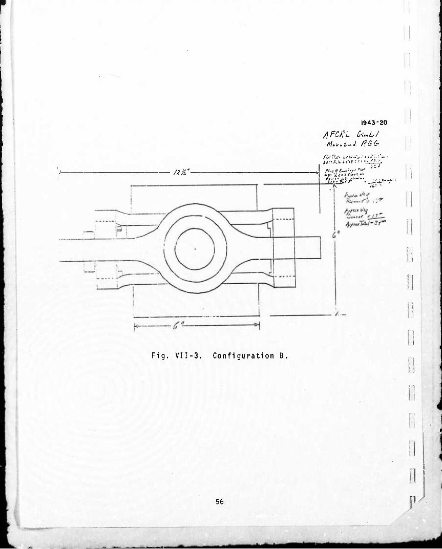
r
UK'
Fig. VII-3. Configuration B.
1943-20
fyfCRl fcmLf
f/y. 'hu //)■/•--V •' •.'- '• *'*■ -
I i
II 11 11
11 11
56
11 P

I I 1
1943*21
•• -■:•;■—
fe^V ;
-' ^ i' / 5 I
v.^' — ■/\\\\NNi u N C\\\\\
■^
If^OlJ^ s\ * •■■■uA—I — i j - -•.- .J..
,T-
r i '' !
€ L^^5l*^77^^^ XysXyj
Fig. VII-4. Configuration C.
57
Amü

Wb-it*
XESTRftiNT WIRB.
rHft/ST Wo
(covf/6vW7iCN "C")
Fig. VII-5. Restraint System Schematic for Tetra- hedron Air Pad Sensor.
i
I
i
i
58
I
i
0 I
I
1 n
•

SECTION VII
configuration is our recommended prototype system. The sensor con-
figuration is described in Section V, RGG Prototype Design Summary,
and the inertia! platform requirements and characteristics are described
in Section VIII, VIALS Requirements.
E. TRADE-OFF COMPARISONS OF ALTERNATE CONFIGURATIONS
This section discusses the many pros and cons of each of the
four above-described sensor configurations. Common criteria which
the four configurations are evaluated against and a summary of the
pertinent comments are shown in Table VII-1. In dome instances, the
space available in the summary table is not sufficient to fully describe
the considerations and hence such details are provided in the following
paragraphs.
1. Angular Rate Isolation Capability
Configurations A, B, and C inherently provide for angular rate
isolation. For Configuration A, computer simulation results show
angular isolation capability is marginally adequate. Very fine adjust-
ment of the ratio of polar to transverse moment of inertia of the float is
required to attain the required isolation. Computer simulation results
are questionable. This is because previous experience in fluid-rotor
gyroscope development has indicated large discrepancies between the
analytically predicted and the experimentally verified damping coeffi-
cient. Also, apparent disturbance torques were observed whose cause
was not understood. This lack of in-depth understanding of the behavior
of rotating fluids weighs heavily against considering this approach at
this time. It was felt that the many other RGG development problems
should be given priority. If a future system application requirement
could be met most favorably with this approach, a separate research
and development program to implement it could then be considered.
59
«^ *m lll^JMll

SECTION VII
For Configurations B and C, the viscous coupling torques of
their air bearing suspensions are mmiacule and hence their inherent
angular rate isolation capability is very good.
In Configuration D, all of the r( quired angular rate isolation
and/or compensation must be provided within the VIALS inertial plat-
form. Our studies show that this is f ntirely feasible and practical.
The required angular rate attenuation of a factor of 14 as shown above
is achieved by substitution of hydrostatic air gimbal bearings. A
detailoH description of this mechanization and the supporting analysis
is provided in Section VIII, VIALS Requirements.
2. Angular Alignment Capability
In Configuration A, angular phase error about spin-axis could
develop. Angular spin rate of the rotor would be closely controlled as
in all other configurations. An additional servo control loop probably
would be required to provide accurate phase alignment between the
rotor and float. This servo would be feasible, but would add additional complexity.
Angular alignment of the sensor arms about axes normal to the
rotor-defined spin axis is accomplished by mass balancing the float
so that its principal axis of maximum moment of inertia is parallt. to
the torsional axis of the sensor arms. Thus any disturbance torques
about transverse axes are balanced by gyrosconic reaction torques in
such a manner that the float maximum moment of inertia axis tends to
align itself with the spin axis. This alignment accuracy can be no better
than that provided by the float mass balance trimming operation.
In Configurations B and C, angular alignment of the sensor about
axes normal to the nominal spin axis must be provided by servo control.
The need for and requirements of this servo control system is discussed in the following item.
In Configuration D, angular alignment about all axes is inherent
because of the direct mounting to the inertial platform stable element.
In all configurations, the angular alignment requirements of the inertial
60
1 !
"!
■I
fl
0 fl /

SECTION VII
platform stable element are similar. Because of the inherent alignment
capability of Configuration D, the inertial platform alignment (and drift)
requirement could be somewhat less stringent than for any of the other
configurations.
3. Sensor Alignment Servo Control
In Configuration A, a spin-axis phase control servo might be
required. Implementation difficulties would arise as noted in the com-
parison table. In both Configurations B and C, it was initially anticipated that
the required angular rate isolation and spin-axis alignment could be
achieved using only passive elastic and viscous restraints. Dynamic
analysis of this passive restraint system revealed two lightly damped
oscillatory modes whose characteristic frequencies were related to
the RGG spin momentum, H, the elastic restraint coefficient, K, and
the RGG transverse moment of inertia, A, as in eqs. (1) and (2).
n p 4 K/H (1)
nN 4 H/A (2)
The normalized damping coefficients, t, , of both of these oscillatory
modes are equal to the ratio of the viscous damping coefficient, D, to
the RGG spin momentum as in (3).
tN = D/H (3)
The equivalent damping time constant, Tp, of the precesoional mode
characteristic frequency, J2p, is defined by (4).
Tp = IT/DK (4)
^ 61
«M
fmk

SECTION VII
Substitution of the appropriate numerical parameters into (4) revealed
a fundamental problem of the passive restraint system; its damping
time constant was in excess of 1000 hr. This calculation is shown in (5).
(2.O39 x 105 g-cm2 x 110 ||^)
(500 dyne-cm-secW 2 x 10 dyne-cm/rad y s 5 x 10 sec (5)
Consideration was given to parametric changes that could reduce this
time constant to an acceptable level of about one minute. This implied
an increase in the DK product by a factor greater than 10 . Angular
rate isolation requirements limit the practical increase of the elastic
constant, K, to less than two orders of magnitude. This implies a
required increase of the damping coefficient, D, by several orders of
magnitude (103 to 10 ). An increase in damping of this magnitude was
not considered feasible, and the passive restraint system was abandoned
on this basis. This led to considering active restraint configurations that
require the addition of torque generators and angle pickoffs between the
RGG stator and its case. The performance requirements of these com-
ponents were investigated, and it was determined that the addition of
components of suitable performance and size was feasible. The dynam-
ics of active restraint configurations based on the angle measurement
only were investigated, and it became apparent that a single-loop design
could not satisfy the conflicting requirements of a low bandwidth response
to external angular rates and a high bandwidth response to torque dis-
turbances. It was concluded that a multiple-loop design would be neces-
sary to provide the required performance. To implement a multiple-
loop design, it is necessary to employ some form of RGG stator inertial
angular velocity feedback. One obvious method is to add two single-
degree of freedom rate integrating gyros to the RGG stator to provide
the rate measurements. Other sensors could be utilized, such as
opposed accelerometers or angular differentiating accelerometers.
A mechanization using any of these types of sensors would result in a
62
I
II ' j
!
i ii
r **m

]
1 SECTION VII
conceptually feasible system; however, it would be impractical, com-
plex, and costly. Another outwardly attractive scheme would be to
employ a passive inertia damper, such as a mercury ring affixed to the
stator. However, preliminary examination of the characteristics of
such a device of acceptable size indicates that it would provide only a
marginally adequate amount of inertial rate feedback. Also, an inherent
problem associated with this device is that an expansion bellows would
be required to accommodate the fluid expansion. Because of the low
stiffness associated with any bellows arrangement, large center of mass
shifts could result, thus increasing the magnitude of vibration-indu jed
disturbance torques. Thus, Implementation of a passive inertia damper
appeared unattractive and at best would probably require a development
effort to assure its feasibility.
4. Sensor Mass Balance
In Configuration A, static and dynamic mass balance of the
float will have to be performed with the flotation fluid surrounding the
float and controlled to the nominal operating temperature. Static
balance can be accomplished using techniques similar to that used for
balancing floated gyros. No known technique has been devised to
accomplish the required dynamic balance, i. e., to bring the float
principal axes into alignment with the sensor arm's torsional axis.
This could be a serious problem and might result in building up
expensive test gear.
Also, in Configuration A, fluid expansion bellows would be
required. Because of the low stiffness of the bellows, a potential
instability of the rotor mass balance might result.
Mass balancing of Configurations B, C, and D appears to be
relatively straightforward.
63
t^^ *mk
mmmm

SECTION VII
5. Vibration Susceptibility
As described earlier, a cylindrical hole passing through the
spherical float of Configuration A is required to provide for C. G.
attachment of the centering pivot. Thus, the arm suspension was
required to be hollow to fit over the center post of the float, and the
quadrilever-type arm support pivots were envisioned as an appropriate
pivot design. Since completing this preliminary design study, it has
been learned that this type of pivot results in an unusually large error
sensitivity to spin-axis translational vibration. This is discussed in
Section XXIV. Thus, this pivot configuration is no longer considered
appropriate. It would appear that for the same reasons the quadri-
lever pivot is susceptible to spin-axis vibrations, any other hollow
arm suspension pivot might very well have similar characteristics.
Design of the gimbal ring of Configuration B to reduce potential
anisoelastic error torques could result in a large, massive structure.
Configuration C overcomes this difficulty because of isoelastic
cnaracteristics of a spherical structure. In Configuration B, rotor
dynamic mass unbalance would have to be very tightly controlled to
prevent self-induced rotational field errors. In Configuration C, such
self-induced errors are minimized. This is because a dynamically
unbalanced rotor will cause a coning-type motion of the sensor spin
axis. It can be shown that no rotational field error results if this
coning motion is purely circular, but it does result if the motion is
elliptical. The motion would nominally be circular in Configuration C,
because of the inherently equal moment of inertia of its stator about
any transverse axis. In Configuration B, the motion would be elliptical
becaise of the anisoinertial properties of the reacting inertia, i.e. ,
the moment of inertia of the stator and gimbal ring is different about
the two suspension axes.
fl 1
D 1
i i n
6. Spin Bearing Selec'ion
In the initial phase of this study when the sensor configuration
selection study was undertaken, the design of <;he spin bearing had not
been started. At that time, a hydrostatic air spin bearing appeared
64
I P
«HI ^m mi g^BBg.

I I I 1 1 1 ]
1 1 ]
1
SECTION VII
the most promising type. Hence, avoiding the high-pressure supply
problem was an important consideration. For that reason, Configura-
tion A appeared the most attractive since increased spring restraint
or mass unbalance disturbance imposed on the inertial platform would
not seriously affect its performance; nor could they directly couple
into the gradiometer. The problem of series feeding an air supply via
the sensor stator suspension bearings to the spin bearing in Configura-
tions B or C did not appear unfeasible, but was an added design com-
plexity. Configuration D would result in a similar design complexity.
The hydrodynamic oil sensor spin bearing design, now com-
pleted, requires no external excitation source. Hence, the above
tradeoffs are no longer a concern.
7. Overall Sensor Size
The table is self-explanatory.
8. Piece-part Fabrication
The table is self-explanatory.
9. Assembly
The table is self-explanatory.
10. Relative Sensor Cost
The table is self-explanatory.
1
11. VIALS Cost
Considerable effort has been expended in conducting surveys of
industry, DOD, and NASA to ascertain the availability of an inertial
platform having the required long-term level and azimuth accuracy
with the load carrying capacity suitable for supporting the required
65
*■* n

^
SECTION VII
three RGG sensors. The results of these surveys have been frustrating
because no system meeting both the accuracy and payload requirements
has been found. For this reason, it has become obvious that a platform
development will be required for an operational system of three sensors.
The performance requirements of the inertial platform for any
of the sensor configurations are stringent. The long-term level and
azimuth accuracy requirements can be met only by the best of inertial-
grade gyroscopes and accelerometers. A very careful design of the
stable element and gimbal structure and gimbal bearings will be
required to limit anisoelastic errors. The additional angular rate
steadiness requirement imposed with sensor Configuration D will
not significantly increase either the development or hardware manu-
facturing cost of the platform. It is shown in Section VIII that incor-
poration of hydrostatic air gimbal bearings in the new platform design
will provide the required angular rate steadiness. Use of air gimbal
bearings is feasible, within the current state of the art, and is not a
major cost ractor. It is estimated that the incremental cost would be
10 to 20% at most. This type of bearing has a significant advantage
over the conventional ball-type gimbal bearing because it inherently
provides a much stiff er bearing, which helps alleviate the anisoelastic
drift errors. Alternatively, compensation of the rotational field error has
been considered. Angular rate sensors having the required accuracy
are feasible. This laternative is treated in more detail in the VIALS
section. A secondary advantage of selecting the Configuration D sensor
is that the long-term level and azimuth accuracy requirement can be
somewhat less stringent than that required for any of the other config-
urations. This is because the other configurations have additional
angular alignment uncertainties due to their additional angular degrees
of freedom.
i
'
i
"1 i
fl
I
1
66 /
—~
- - A "— tmimamä
SECTION VII
There would be no major differences in the requirements
imposed on the vibration isolation mount of VIALS for any of the
sensor configurations. Because of the size differences between sensor
configurations, the size and payload weight would be somewhat altered,
but this is inconsequential in terms of technical feasibility or cost.
1
I F. CONCLUSION
I
The dominant criteria used in selecting the prototype sensor
configuration are complexity and cost effectiveness of the operational
gradient sensing system. Solution of the angular rate isolation problem
is the primary consideration affecting this selection. Schedule
requirements and budget limitations preclude selection of a system
configuration requiring significant development effort or high technical
risk items.
Complexity and technical risk considerations rule out
Configuration A. Configurations B and C require either a complex
mechanization using two inertial angular velocity feedback sensing
devices per RGG sensor (a total of six devices per system), or they
involve development of a passive damper whose technical feasibility
and practicality are questionable.
Configuration D imposes the least technical risk and cost in
development of the R&G sensor. The additional angular rate steadiness/
compensation requirement imposed on the VIALS inertial platform
does not represent a significant incremental cost or technical risk.
The simplicity and cost effectivenss of the total operational system
is by far the greatest for Configuration D, hence Hughes has selected
Conliguration D as the prototype sensor configuration.
67

SECTION VII
0 b
I a 3 0 M **
§ I 0 I
w
PQ
I 1 SI
'S < O K
3|
31 ss >- i
tl o
i) ^ i«
111
5 -
E^
■ o!:
« > • ~ > «
- M • S 0 i ,- .. "i i
.»12 III!
E 'S
X ■
* •, E K-O
5 7 * aiJ!
a^ i
^: ^
£■00
Mi
iii
4 »Dl
•Si o ». 3 ti
r, ^ si
1 3- J 7 « E i-o
IM 4 0
- 9 IB
ii US 1= <<
o-;,
o U 0
BJ
a;E o £ c
&61
i. 3 C »
S Ü « 3 o c c u i.. - _ ^
Pi*! « s 11
c « J» * * U *" »
•■ 3 " >.
> S • ; II c r 5 > ? X . 2 E S-'S i J if0 . o tp s
■ IN £
«I« 5 ■« •
■» -:
■ 'S o- S oo
fi K 1 Ji ■ 3 6.0 « >.
« o « *. 5
glsil
h U u
11«
III III
K 0 Ä- 4 ^ h >- ««SO
6 >-o g Ä « •• w
<« C w c *, •> c 5 E-EE^ illll
3 a ti
9" i ■
JB 1
V P.
15
v 2^ •o 9
"■,8
p 93
„ o j . C II . 3 o c c g u 2 << "
••£■08 «ill
81
S3
:*5
9 « k 4 X II u^ ■D
■£3
« » - c 2 : si
^IE SH ilJ! 3' «SS "SIR
Sfil
■ E _ c ■sir 0
81
n. v c 0
: C 11 ■«
:^i2
'ah il| * JS ti
b « «.
•" 0 o
S - o 3 W - U > TJ
«il u 0 c
s» °
j j! x
0 0 ■ s. G -5 0 c
ififj
» .
o o m O c «■
I
V
•o o SCE
c Ä
« u <!
Hi ö " « 4; c ** ir« 3
■/I
I ij si ■■
si u 11
II «0 5 c E l?|
Eit « u <!
II i 5 ■ "j
iss
j* o -c
<!- 0 3 0
" • c . "•■■ s ■ Is!*
C M
» .« fl
is M ^SSos iSli
= 33
£ i I -3 »I U. a C u o „
Man
Ex:
JxiA * O
hi C n
~ J! o
it j E * MA 5 ■ t
i c »1
fli
h ■] I &!» • o* c
3 N J
< i;'5
111. = «■25 J-o - « e « 3 « U) Q • x
5" 3 • * ll
ill
X
o " c
B.|t .2oS • ~ B O >. »
16? • " O
Ei« k >■ ■ «ig i vs o u tt ~ S u O "O X
H a 5x . k M •«
VX v
X O " C C II
is»
F« 0 "Wo C »I o-
"'S
0 >- c *■
— w m 4 « « c L . t „
■^ ** u
"£ S2
O J « ^rt C tu tmp 0 ■ vO jj P «f
■C5
O "O
Ik" .01.
■0 7 « o
E- !; • 11
i
i
!
fl 1
fl i
i £=!; • s k .s S " •
so s „ i
t 3
si I- Id Ov>
ni i
68
I /
m^^

I
I I ]
1 ]
I I T B
i
i i i i
SECTION VII
a <
0)
c
u
£ £
d o en
•H U <i
I o U
0 V
TJ R) U H
§ Ü u
id c 0 u i
69
^MÜ

I I I 1 1
1
I I 1
I
SECTION VIII
VIBRATION ISOLATION, ALIGNMENT, AND LEVELING SYSTEM
A. GENERAL
The need for a vibration isolation, alignment and leveling
system (VIALS) for support of the three-RGG sensor cluster has been
recognized for some time. Earlier studies conducted by Hughes have
ascertained the requirements and characteristics for the VIALS. Two
basic functions are provided by the VIALS: (1) establishment of a
gradient measurement reference frame via providing azimuth and level
stabilization of the three-sensor cluster, and (2) attenuation of trans-
lational and angular vibrations to reduce induced errors resulting
from vibration sensitivity of the RGG to these motions.
These earlier studies have considered the tradeoffs of various
mechanization approaches. These studies resulted in establishing a
basic building block approach to provide the two basic functional
requirements. It consists of the following: The three sensors are
mounted to the stable element of an inertially stabilized three-axis
platform. The platform in turn is supported by a softly sprung
vibration-isolation mount, which is affixed to the carrying vehicle.
This softly sprung mount provides for isolation of translational vibra-
tions induced by the carrying vehicle. It also serves to attenuate
vehicle-induced angular vibrations. The three-axis platform provides
long-term azimuth and level stabilization of the RGG cluster.
Contractual requirements of this Phase I study have been to
determine the characteristics and requirements of the VIALS and to
demonstrate that any of its components are within the current state of
the art. As such, detailed design of the VIALS was not carried out.
The Hughes recommendation for the VIALS configuration, although not
backed up by an in-depth detail design, will be referred to as the
prototype VIALS configuration. (It is referred to as "prototype" in the
^ Preceding page blank
71
—
tmsmem

mma
•
SECTION VIII
sense that it is compatible with our selected prototype RGG sensor
configuration).
B WORST CASE ENVIRONMENT
Hughes has selected an airborne environment typified by a
KC-135 aircraft as the "most critical application. " This is discussed
in the Technical Report No. 1. Therein, we have presented data show-
ing the power spectral density for aircraft angular acceleration and for
aircraft angular rate. A minor transcription error was made in the
presentation of these data in that report. Hence, the corrected data is
re-presented herein (see Figs. VIII-1 and VIII-2).
C. VIALS REQUIREMENTS FOR PROTOTYPE RGG SENSOR
The performance characteristics and design requirements of
the vibration isolation mount and the stable platform are stated herein.
These are the minimum requirements necessary to insure that opera-
tion of the RGG sensors in the aircraft environment for durations up to
10 hr will result in measurement of the gravity gradient tensor elements
to an accuracy of 1 EU, 1 sigma. These requirements are presented
in a specification format.
1. 0 Vibration Isolation, Alignment and Leveling System
This specification states the requirements for a vibration
isolation, alignment and leveling system to be used tc support three
orthogonally mounted RGG sensors. This system shall consist of a
vibration isolation mount subsystem and a stabilized platform subsys-
tem. The requirements stated herein shall apply for the total assembled
system consisting of the vibration isolation mount, the stable platform,
and three RGG sensors including sensor electronics. The system shall
be capable of meeting the specified performance throughout a
10, 000-hr operating life, with a minimum of '000 warm-up cycles,
72
!
I
i
"I
[]
I
i
i
1 P
<*m **U

t
2075-42
I
Q
O
0.01 0.1 I 10
log FREQUENCY, Hz
000
Fig. VIII-1. Acceleration Power Spectra.
73
■ äMM^MOHl

I
2075-41
I 10
log FREQUENCY, Hz
1000
Fig. VIII-2. Angular Rate Power Spectrum.
74
:
fi
B
^- worn

w^*
1 1 SECTION VIII
at any time during a 2-year period following delivery, when exposed to
any and all combinations of the aircraft operating environment specified
herein.
2. 0 Environment-Operating
The VIALS system will be used to support the three RGG
sensors for collection of gravity gradient data in a jet aircraft. After
takeoff and climb to cruise altitude, the aircraft will be flown in a
straight and level cruise condition during non-turbulent weather con-
ditions while data is being taken. The airborne operation is at a
subsonic speed, approximately 400 to 500 mph at a constant cruise
altitu-ie of between 25, 000 to 35, 000 ft in a mulciengine jet aircraft
such as the KG-135. A nominal cabin temperature of 720F ±3° will be
maintained. The aircraft motion environment shown in Figures VIII-1
and VIII-2 is applicable and applies to all axes. A cabin pressure of
between sea level and 10, 000 ft equivalent pressure altitude will be
maintained at all times.
3. 0 Functional and Performance Requirements
3. 1 Vibration Isolation Mount - The vibration isolation mount shall
support the weight of the stable platform and 3 RGG sensors and sensor
electronics. It shall provide isolation in six degrees-of-free^om of
the isolated load with respect to the aircraft mounting reference. A
right-handed x, y, z aircraft body-fixed orthogonal reference coordinate
system centered at the aircraft mounting reference is defined with x
along the aircraft's fuselage reference line, z along the nominal vertical
and y normal to x and z. The isolated load is defined to consist of the
portion of the vibration mount rigidly affixed to the base of the stable
platform, the stable platform, and its i RGG sensor and electronics
payload. The mount shall provide three translational degrees-of-
freedom along x, y, and z and three rotational degrees-of-freedom
1 76
m^m^gm ^■ft

^*
SECTION VIII
about x, y, and z of the isolated load with respect to the aircraft
mounting reference.
3. 1. 1 Load Capacity and Dynamic Range Requirements - The vibration
isolation mount shall provide the specified vibration attenuation while
supporting its payload and v/hile being exposed to the vibration spectra
specified in paragraph 2. 0. Additionally, it must provide the specified
vibration attenuation and not exceed the inertial and elastic coupling
limits specified in paragraph 3. 1.2 when exposed to aircraft maneuver
loads of 0. 1 g.
3. I. 2 Inertial and Elastic Coupling - The vibration isolation mount
shall limit inertial and elastic coupling between the six degrees-of-
freedom as required below.
3. 1. 2. 1 Elastic Center - The vibration isolation mount shall have a
nominal elastic center defined by a point such that application of an
incremental force (not to exceed 0. 1 g maneuver load factor) at that
point in any direction shall result in pure translation of that point and
no rotation about that point of the isolated load with respect to the air-
craft mounting reference.
Deviations from this defined nominal elastic center shall be
limited as follows. The elastic center may not vary by more than
±0. 2 in. from its average location as a function of the direction of the
incremental load. Its average location shall be defined by determining
the average of the elastic center locations found by applying 0. 1 g
incremental loads, one at a time, in each of the three cardinal x, y,
and z directions.
3. 1.2. 2 Mass Balance - The vibration isolation mount shall be equipped
to provide for mass balancing of its isolated load. This required mass
balance adjustment equipment shall be capable of adjusting the isolated
load's center of mass to within ±0. I in. of the average elastic center
as defined in paragraph 3. 1. 2. 1.
76
I
1
11
1
0 fl
i i
fl
mm *mk mmm

■^■Mvw^—*
a
i
D I D r r r i [ i i i i
i
SECTION VIII
3. 1. 3 Translational Vibration Attenuation - The vibration isolation
mount shall provide for isolation of translational vibration in all three
axes. The translational isolation performance in any axis shall be
equal to or exceed the performance characterized by a second-order
linear system having an undamped natural frequency of 1 Hz and a
damping ratio of 0.4.
3. 1.4 Rotational Vibration Attenuation - The vibration isolation mount
shall provide for isolation of rotational vibration about all three axes.
The isolation performance in any axis shall be equal to or exceed the
performance characterized by a second-order linear system having
an undamped natural frequency of 2. 5 Hz and a damping ratio of 1.0.
3. 2 Stable Platform - The stable platform shall meet the following
performance requirements while supporting the three RGG sensors and
electronice. and when mounted on the vibration isolation mount whose
characteristics are specified in paragraph 3. 1 above.
3. 2. 1 Reference Stabib nation Axes - The stable platform shall provide
three-axis stabilization such that a locally level, true north referenced
stable element orientation is maintained. (It is only required that a
true north reference be available, e.g. , an "azimuth wander" system
mechanization is fully acceptable. )
3.2.2 Angular Freedom - The stable platform shall be capable of
accommodating aircraft motion excursions of ±30° M pitch and roll
while in any heading orientation. Aircraft heading variations of more
than 360° shall be accommodated.
3. 2. 3 Gimbal Readout - Angle transducers providing an output signal
proportional to gimbal angle for each of the three axes will be
required for compensation of the RGG output due to mass proximity
effects. These transducers shall have an over-all accuracy of at
least ont [\) arc minute. Note that this requirement is in addition to
77

"V-
SECTION VIII
any resolvers associated with the stabilization servo loops of the
platform.
I
!
}
3'2'4 Angular Alignment Accuracy - Initial alignment accuracy and
allowable drift limits are as specified below.
3-2.4. 1 Platform and RGG Initialization - The accuracies required for
initial alignment of the three-sensor cluster are as follows:
Vertical: 2.5x10 radian, 1 sigma, with respect to the local plumb-bob vt rtical.
.4 Azimuth: 5x10 radian, 1 sigma, with respect to the
reference stabilization axes north reference.
After initial alignment of the three-sensor cluster, RGG
initialization will be accomplished. This RGG initialization process
may require up to one hour to complete. The platform drift and angular
motion steadiness requirements of paragraphs 3.2.4.2 and 3.2.5 shall
apply during this RGG initialization period. No retrimming or adjust-
ment of the stable platform can be allowed at any time during the ensuing
10-hr operational run after RGG initialization has commenced.
3' 2-4- 2 Allowable Drift - The stable element angular orientation shall
not drift from the initially aligned reference stabilization axes orienta-
tion by more than the following amounts for flight durations of up to 10 hr;
_ 5 Level: 5x10 radian, 1 sigma.
Azimuth: 5 x lO"4 radian, 1 sigma.
3. ;. 5 Angular Motion Steadiness - In addition to the long-term drift
stability specified in paragraph 3.2.4.2, angular oscillations of the
stable element shall be limited by the following cri'eria.
3.2.5.1- The integral over all frequencies of the angular rate power
spectral density about any axis of the three-sensor cluster shall not - 1 U 2
exceed 10 (rad/sec) .
1
i
0
"I
0 i
i
[1

•^T"
'
I 1
I
SECTION VIII
3. 2. 5. 2-The requirement specified in paragraph 3. 2. 5. 1 above is a
simplified statement of the angular rate steadiness requirement. The
above requirement is based upon somewhat conservative assumptions
regarding spectral co- and cross-correlations of angular rates about
the three orthogonal axes. In Section IX, "Error Analysis" and in
Technical Report No. 1, pp 38-46, "Covariance Functions of the
Rotational Field Errors of the RGG, " the precise relationship t «tween
these angular rate spectral properties and the resultant gravity
gradient tensor element errors are defined. It is required that the
rotational field error, induced as a result of angular rate jitter of the
three-sensor cluster, of any of the gravity gradient tensor elements
be limited to 10" 10 (rad/sec)2, 1 sigma. If desired the above require-
ments may be substituted for the simplified requirement of
paragraph 3. 2. 5. 1.
3.2.5.3 Angular Rate Compensation - The angular rate steadiness
requirements of paragraph 3.2.5.1 or 3.2.5.2 may be relaxed if a
suitable system of angular rate sensors is provided. This system of
angular rate sensors shall be capable of measuring and providing com-
pensation signals to each RGG sensor with measurement and data
processing accuracies consistent with the angular rate steadines
specified in paragraphs 3.2.5.1 or 3.2.5.2.
\
3.2.6 Stable Platform Computer - A stable platform computer will be
required whose accuracy is compatible with meeting the angular
alignment accuracy requirements of paragraph 3.2.4 and the angular
motion steadiness of paragraph 3. 2. 5.
I I I
3. 2. 7 Payload Description - The weight and size of the three RGG
sensors and their associated stable element mounted electronics is
as follows:
79
i^M ^m

SECTION VIII
Sensor:
Electronics:
Compensation Accelerometer;
Weight - 25 lb
Size - 6-in.dia x 8-in. long cylinder
Weight - approx 10 lb
Size - volume sO. 2 ft3 may be packaged to accommodate stable element design
3 required. Wt - 1 lb
Size - 2-in. dia x 1-in. long
3. 2. 8 Power and Signal Transmission - Slip rings or their equivalent
will be required to transmit power to and signals to and from the
specified payload equipment as follows:
ac power: a. 100 V, 60 to 100 Hz, 2-phase (90° phase shift) power
0. 25 A run per leg plus 0. 3 A return.
b. 28 V, 400 Hz, 3-phase, 100 W.
dc power: 2 A at 28 V dc.
signals: Provision for approximately 32 signal channels.
3. 2. 9 Mechanical Impedances:
3.2.9. 1 Vibration Isolation Mount - The stable platform shall be
capable of meeting the performance specified herein when mounted on
the vibration isolation mount specified in paragraph 3. 1.
3.2.9.2 Reaction Torques from Payload
a. Sensor Rotor Mass Unbalance - Each sensor's rotor mass unbalance shall not exceed 7. 5 x 10⁻⁵ Ib-in. Each sensor is operated at a nominal spin frequency of 105U rpm.
b. Sensor Angular Momentum - The angular momentum of each sensor is 2.24 x 10⁷ gm-cm2/sec.
80
!
1 I
n
n
i
i
1 /
MMB

I
■
r
i
r i:
i \
i
i i i i
SECTION VIII
4. 0 Test Requirements - Due to the preliminary nature of this
specification, no detailed qualification or acceptance test requirements
are included herein. Because the intended application of this system
is for mulitary purposes, appropriate military specifications will be
applicable.
D. BASIS FOR VIALS REQUIREMENTS
This section summarizes the basis of the important performance
requirements imposed by the above VIALS specification.
The vibration isolation mount is required primarily to attenuate
aircraft translational vibration. The predominant RGG sensor errors
caused by translational vibration are arm differential mass unbalance
and arm anisoelastic properties. A secondary benefit of the vibration
isolation mount is to reduce the oscillatory angular motions of the air-
craft from the base of the inertial platform. This aids ^n reducing
friction-coupled disturbance torques to the platform's stable element.
The requirements to minimize the inertial and elastic coupling
are necessary to: (1) limit the amount of angular motion of the stable
platform's base induced by aircraft translational vibration, and (2) to
limit the amount of translational motion of the stable platform's base
induced by aircraft angular vibration.
The specified 1. 0 Hz translation natural frequency with 0.4
damping ratio second order transmissibility requirement limits the
translational vibration spectra of the stable platform. Similarly, the
specified 2. 5 Hz rotational natural frequency with 0. 4 damping ratio
along with the specified elastic center/mass balance requirements
limits the rotational vibration spectra. A system designed with these
specified characteristics will ittenuate the aircraft translational and
rotational vibration spectra as shown in Figs. Vni-3 and VIII-4. The
resultant translation spectra has been used to estimate the RGG errors
associated with translational vibration. These results are shown to be
within the required limits consistent with the over-all accuracy
requirement of 1 EU in the Error Analysis, Section IX.
81
*M* mmm—mmmm

m V ^^
SECTION VIII
The stable platform is required to provide azimuth and vertical
stabilization and the final stage of angular rate isolation. An analysis
of the errors resulting from initial misalignment and drift of the stable
platform is shown in Section IX. Briefly, angular orientation errors
cause fictitious inputs to the gradiometer which result in apparent
gradient component values that would be interpreted as true gravity
gradient signals. Because of the relatively large nominal gradients
of the earth (3000 EU vertical and 1500 EU horizontal), relatively large
errors of the off-diagonal gradient tensor components (which are
proportional to the sine of the tilt error angle times these large nominal
gradient values) can result.
z ■s.
o ui a
ID-
10"
10
10
-•
10
10"
-ll
001
i0Ti-*0
\ _ \
N
AIRCRAFT
INERTIAL PLATFORM BASE
0.1 I 10
lo« FREQUENCY, Hi
100 1000
I
I
1
"I
"i
0
II
Fig. VIII-S. Acceleration Power Spectra.
82 a z'
i^a

• " ' 'P'
1
r r
i i n i:
[ i i i i
IO-I-
lO-' -
z
IS 10
d
o:
? IO-0
o-|2l-
10 -14
0.01
207S-59
1 I
\\
1
1 1
\ \
\\
'■—
_. V
1
1
1
AIRCRAFT
V-
^
—— ——• INERTIALPLATPORMBASt \ ^
i 1 1 1 0.1 I 10
log FREQUENCY, Hz
100 1000
Fig. VIII-4. Angular Rate Power Spectrum.
83
- -"- ■atffttftfl

^^
SECTION VIII
The specified angular rate steadiness requirement is impcaed
primarily to limit rotate jnal field errors of the gradiometer. The
specified requirement translates to limiting these rotatiomd field
errors of the tensor components to 0. 1 EU, 1 sigma.
The requirement for ±30° gimbal travel in pitch and roll is
consistent with aircraft attitudes which can occur during takeoff and
landing. The full freedom in azimuth is required to not limit the
survey aircraft's heading. During an operational run, it might be
desired to retrace a course or fly a criss-cross pattern for purposes
of data correlation.
Gimbal angle transducers are required to compensate for the
effects of proximate masses aboard the aircraft as heading and attitude
change. The influence of aircraft proximate masses has been studied
in detail and is discussed in the September 1971 HRL Technical
Proposal. Appendix I (see Section V-D). This study shows that the
primary item of concern is the proximate mass effects of the stable
platform gimbals.
E. VIBRATION ISOLATION MOUNT DESIGN CONSIDERATIONS
84
i
i
fi
Hughes has conducted earlier studies of three types of softly
sprung vibration isolation systems. Detailed results are shown in the
September 1971 HRL Technical Proposal, Appendix F (see Section V-D).
These studies have considered three types of spring-damper elements
and several linkage arrangements utilizing these elements. The three
elements considered were: (1) a coil spring v'ith a parallel viscous
damper, (2) an elastomer element (Bungee chords), and (3) an air-
column isolator.
The results of these studies have indicated the use of an air-
column spring-damper element to be the most appropriate. Elements
of this type are readily available. They are in widespread usage in
bus suspension systems. Laboratory vibration isolation test tables
using the bus type suspension for support of a granite-top table, with a
pneumatic servo controlled leveling feature, are available from several
v
MMH^M

*F
1
l
I ^
SECTION VIII
manufacturers, including Modern Optics Corp., Barry Corp., and
Newport Research Corp. Barry Corp. also makes a smaller unit
referred to as Barry Servo-Level, which also has a similar pneumatic
servo that utilizes a simple mechanical linkage feedback control. All
r air-column isolators of th;3 type have the desirable characteristics
of providing vibration isolation efficiency equal to that of a virtually
unuamped second-order system at high frequencies while providing
near critical damping (transmissibility of less than 1.5) at the system
resonant frequency.
An arrangerrent of six of these isolators in an axisymmetric
linkage is proposed. The arrangement is depicted in Figure Vni-5.
Each end of each isolator element is connected by a spherical joint,
one end to the stable platform and its opposite end to the aircraft floor.
p This arrangement is novel, because if the axis of each adjacent
isolator is extended, they meet at a point. These intersections of each
.. adjacent set of isolator axes form six of the eight corners of a cule,
while the isolators themselves lie along six of the edges of the cube.
The dotted lines of Figure VIII-5 indicate the remaining six edges of
the cube. Therefore, any given vibration force directed parallel to
one ojE the edges of this cube cause equal loads on the two isolators that
lie along these parallel eJ^»«- The result of such an arrangement is an
isoelastic structure in the sens" that it has equal translational spring
(rates in all directions of force application. Similarly, it has equal
rotational spring rates, regardless of torque direction. By proper
_ placement of the center of mass of the supported load, this structure
I also will not induce angular rates into the load caused by linear vibra-
tions of the vehicle, nor will it induce linear vibrations into the load
i caused by angular vibrations of the vehicle.
Each of the si * isolators is supplied with air via a simple
1 mechanically actuated servo valve. The mechanical linkage is
arranged so that if the isolator extends beyond a certain point in one
■ direction, the valve bleeds air out of the isolator, and if the isolator
extends beyond a certain point in the opposite direction, the valve bleeds
supply air into the isolator. The time constant of this servo action is
85
M^

I ^p ^ ' • 'P '
AIR COLUMN ISOLATOR
TOP VIEW
ISOMETRIC VIEW
FRONT VIEW
R
Fig. VIII-5. Six-Element Axisymmetric Linkage Air Column Vi bration Isolation Mount.
!
86
1 T
•

1 I
r. B [ i: i i i. i:
i i i i
SECTION VIII
long compared with the period of the vibration disturbances of concern.
The predominant error sensitivity of the RGG is caused by vibration at
one and three times its spin frequency of 17. 5 Hz. In the previous
subsection, it was indicated that sufficient isolation would be provided
with a linear second-order system with a natural frequency of 1. 0 Hz
and a damping ratio of 0.4. Use of the air-column element with its
natural frequency set at 1. 0 Hz would provide more than adequate
attenuation of the sensitive frequencies of 17. 5 and 52. 5 Hz.
F. STABLE PLATFORM DESIGN CONSIDERATIONS
As discussed in Section VII, it has been determined by surveys
of industr*/ and Government inventories that a stable platform meeting
the combined long-term accuracy and payload requirements is not
currently available. It has, therefore, been assumed that a platform
development will be necessary to meet this dual requirement.
A requirement of this study is to demonstrate the current state-
of-the-art feasibility of components of the required VIALS. Two areas
of the stable platform performance requirements were considered
potentially difficult: (1) the level and azimuth accuracies, and (2) the
angular rate isolation requirements. These subjects are discussed
below. These topics are followed by a discussion of the design approach
and a brief physical description of the recommended operational system
prototype design concept.
1. Level and Azimuth Stabilization Accuracy
Three approaches are available to provide the required level
and azimuth accuracies. These methods consist of: (a) a pure
(unaided) inertial mechanization, (b) an aided inertial mechanization,
and (c) a master-slave mechanization.
a. Pure Inertial Mechanization
The gyros and accelerometers necessary to produce the
level and azimuth stabilization accuracies for a pure inertial
87

^P"GP ^
SECTION VIII
mechanization approach are high quality inertial components, but they
are well within the state of the art.
The required inertial component accuracies would be typified by the following performance parameters:
Gyros
Systematic drift rate uncertainty ±0. 003o/hr
Random drift rate ±0. 003o/hr
Accelerometers
Long-term bias stability ±10"4 g
Bias repeatability, warmup to warmup ±5 x 10 g
The AN/USQ-28 Geodetic Mapping and Survey Subsystem uses a Bell
Aerosystems Hipernas II-B stable platform with a Nortronics CP-720
digital computer. This system has demonstrated 10 arc sec, 1 sigma
(*5 x 10⁻⁵ rad) vertical accuracy and better than 60 arc sec
(«2. 5 x lO"4 rad) azimuth accuracy in numerous flight tests on an
RC135A aircraft. Results of this flight test program conducted at
Eglin Air Force Base, Florida, are documented in a Bell Aerosystems
report "Technical Note, Hipernas IIB 1969 Flight Test Performance,
Eglin Missile Range", Report No. 6208-936002, February 1970. A
copy of the Bell Aerosystems Hipernas II-B specification is reproduced
herein as Figure Vm.6. It is understood that seven of these systems
are presently available for appropriate Department of Defense programs.
These inertial sensors and computer, mounted on a suitable RGG stable
platform, would provide the necessary level and azimuth accuracy.
Several other classified inertial navigation systems which are
now in operational usage are known to exist and could provide the nec-
essary puro inertial level and azimuth accuracies. Performance
specifications for these systems are not shown to avoid the necessity
of placing security classification restrictions on this report.
b. Aided Inertial Mechanization
An aided inertial system utili7i:ig high precision Loran,
Transit, Doppler Navigation Radar, Position Fixes, and Star
88
I
1
n
I
I l
m*M ft

V ■"
(J) BELL AEROSYSTE/VIS CO/MPAPUY
ni. mPERNASIIB
A. SPECIFICATION
The following is a specification defining the primary characteristics of the Hipernas
IIB IRU:
1'. Performance
Position error rate (CEP)
Velocity error dc ac
Azimuth
Verticality
Gimbal readout accuracy
2. Number of gimbals
3. Reaction time
4. Weight
5. Size
6. Inherent MTBF
7. Packaging
8. Power Requirements
Power Consumption:
9. Mechanization
0,1 n.ml./hr for 12 hr (See Figure III-l for typical per- formance. Additional data in Appendix B)
< 1 ft/sec 0.001 ft/sec
<60 arcsec In 10 hr
10 arcsec rms In 30 hr
30 arcsec max error
three
<2.5 hr
150 lb
3,7 cu ft
500 hr
Discrete components
120/208 v rms, 3 phase, 400 Hz primary power in accordance with MIL-STDr704, provided the ab- normal voltag» transients are be- tween limit;. 3 and 4 of that standard and do not occur more often than once per hour
ISOOw start and warmup
450 w operate at 25°C
See Appendix A
4
Report No. 6208-936001
Fig. VIII-6. Hipernas IIB IRU Specification.
IU-1
89
m*m Mrt

SECTION VII
Trackers can be utilized. The extent to which these aids can reduce
the accuracy requirements of the inertial sensors is dependent on the
particular type of aids used, their inherent accuracy, and the degr..e
of sophistication used to "marry" these aids to the pure inertial system.
Incorporation of such aids adds considerably to the over-all system
complexity. Because several pure inertial systems have the proven
capability to meet the RGG requirement, a pure inertial mechanization
is favored by Hughes.
c. Master-Slave Mechanization
This mechanization approach is attractive especially if
the survey aircraft or carrying vehicle has or must have a primary
inertial navigation rystem aboard for providing precision navigation
station-keeping information. If this system itself had the specified
long-term azimuth and level accuracy, it would serve as the master
system to which the RGG stable platform would be slaved.
With this approach, only modestly accurate gyros and acceler-
ometers would be required for the RGG stable platform system,
typically level axis gyro bias stability of 0. Ul deg/hr, azimuth axis
gyro bias stability of 0.02 deg/hr, and accelerometer bias short-term
stability of 1 x 10"^ g. The RGG platform would be a Schüler tuned
mechanization. The slaving of the RGG platform to the master naviga-
tor would be accomplished using Kaiman filter technique. The number
of error states employed in this Kaiman filter probably would be about
eight or ten. The digital computer requirements to implement the
required number of Kaiman filter states would be modest. This filter
would be implemented as part of the RGG platform management com-
puter or possibly could be programmed in the management computer of
the master navigator.
This master-slave approach could result in a satisfactory and
attractive over-all system mechanization. Detailed studies would be
required to determine the specific mechanization requirements of this
approach and to compare its cost effectiveness to that of the pure
inertial mechanization once the specific RGG application is defined.
90
i
i
n
i
s

•^^
I I I
[ [
i
r [ !
I 1 I I 1
SECTION VIII
Z. Angular Rate Isolation Feasibility
Hughes has performed studies to determine the potential
problems which might arise if the bulk of the angular rate isolation
capability is to be provided by the RGG stable platform. In addition
to the studies conducted by Hughes, an outside firm, Acroflex
Laboratories, Inc., Plainview, Lorg Island, New York, was hired to
consult on this over-all angular rate isolation problem, Aeroflex was
chosen as a consultant because of their very applicable experience in
similar systems. They have developed many camera mounts and other
large-payload airborne stabilization systems. They also have
developed a product line of large capacity dc torque motors which are
required by such systems.
The Hughes and Aeroflex studies revealed four potentially
significant sources of platform stable-element disturbances:
a.
b.
c.
d.
Platform stable-element and gimbai mass unbalance
RGG rotor mass unbalance
Stabilization gyro signal noise
Platform gimbai bearing coulomb-type friction torque.
The most predominant disturbance source would result from
platform friction if ball-type platform gimbai bearings were to be used.
In Section Vh the amount of angular rate disturbance that could occur
has been estimated to be approximately 14 times the amount that can
be tolerated. Hence, ball-type bearings were ruled out. Several
alternate gimbai suspension techniques have been considered. These
all employ the use of hydrostatic gas bearings. Three types of
mechanizations were considered: One suspension essentially replaces
the conventional three-axis platform ball-type gimbai bearings with
air bearings; the second type would utilize a hemispherical knuckle
air bearing that would provide the required three-axis isolation;
the third type would utilize a conventional three-axis ball bearing
gimbai platform with a hemispherical knuckle air bearing between the
91
v :
tfü jtm
mm 'W~
SECTION VIII
stable element of the ball bearing platform and the gradiometer and
inertial sensor payload.
In any of these mechanizations, some form of slip rings or
t' eir equivalent are required to provide power inputs and signal inputs
to and signal outputs from the inertial sensors and the three RGG's
mounted on the stabilized element. Low-level signals cculd be trans-
mitted via a telemetry link; however, the power inputs would require
the use of slip rings or direct wires. Either would result in
undesirably large disturbance torques. The use of slip ring follow-up
servos, which essentially reduce the coulomb friction torque to zero,
appear to be the best solution to this problem. Implementation of the
slip ring follow-up servo is direct and straightforward for the three-
axis gimbal bearing mechanization.
It is felt that torquing and angular motion detection of the three
axes of freedom of the hemispherical air bearing mechanization would
present very difficult design problems because of the relatively large
(±30°) roll and pitch freedom and full azimuth freedom requirements.
This problem would be reduced if the third mechanization were
employed. However, even then, providing the power and signal
communication between the three-gimbal platform stable element and
the gradiometer and inertial sensor payload would be difficult.
Because of the above considerations, the three-gimbal air
bearing approach has been selected as the preferred mechanization
approach for the operational system prototype stable platform.
To estimate the magnitude of the four disturbance sources
mentioned earlier, the pertinent design characteristics of the prototype
stable platform were required. A preliminary design of the prototype
platform was made, and estimates of these characteristics were gen-
erated. A description of the prototype platform and its design char-
acteristics are presented in the next subsection.
The basis of computing the disturbance torques, the angular
rates they produce, and the resultant rotational field errors of the
gravity gradient components follows.
92
I
i
i
I
I
11
r

■»■•■
SECTION VIII
1 1 ß
I I I 1 1 i;
a. Platform Mass Unbalance
The presence of gimbal bearing coulomb friction torque
masks the induced mass unbalance torques created by the earth's 1 g
field. Hence, because of the very low friction torques associated with
the use of air bearing gimbals, significantly better static mass balance
of the gimbals and stable element can be achieved compared to a ball
bearing gimbal suspension. As shown in a subsequent section, residual
coulomb-type friction torques will remain even with air gimbal bear-
ings. The estimated magnitude of these residual normalized friction
torques (ratio of torque to platform moment of inertia) is -4 2 l.H x 10 rad/sec . Ideally, the mass unbalance of the platform
gimbals and stable element could be adjusted down to a level equaling
this residual torque. Conservatively, it is estimated that adjustment
to wit*1- i ten times this level could be achieved, resulting in a nor- -3 2 malizeu mass unbalance torque ratio of 7. 8 x 10 rad/sec per g.
The resultant rotational field error caused by angular rates
induced by the aircraft vibration acting on the platform mass unbalance
is estimated as follows. The power spectral density of the platform's
mass unbalance normalized disturbance torque is given by the product _3
of the square of the normalized disturbance torque ratio, 7.8 x 10
rad/sec per g, and the estimated platform base acceleration power
spectral density, S., from Fig. VIII-3, or
(7.8 x 10"3)2 S, (1)
disturbance torque, H-, has been estimated and is shown in Fig. VIII-8.
The power spectral density of the platform angular rate, Sw, is obtained
as shown in eq. 2.
12
d Sw = |H(j2Trf)|2ST (2)
The variance of the platform angular rate, <rw , is obtained by
integration of its power spectra over all frequencies as shown in
eq. 3.
93
^Mii

SECTION VIII
H{j2ff£)rST df (3) I id
The platform stable element angular rate variance has been
evaluated using the estimated normalized mass unbalance and the data -14 2 of the two figures. The resulting variance is 27. 8x10 (rad/sec)
_7 or a standard deviation of 5. 3 x 10 rad/sec.
The worst case gradient tensor component error due to this
rotational field input can be approximated by eq. 4.
= o-. (4)
Thus the estimated rotational field gradient error due to platform mass
unbalance is 27.8 x 10'14 (rad/sec)2 x 109 EU/sec"2 = 0.000278 EU and
is negligible.
b. R. G. G. Rotor Mass Unbalance
The RGG rotor mass unbalance is expected to be trimmed
and to remain stable within 2 |JL in. , which corresponds to a pendulousity
of 0. 0? gm-cm. Results similar to this have been achieved on the
earlier Hughes RGG experimental hard bearing sensor. The small
centrifugal force resulting from rotor mass unbalance can create a
distrubance torquo at the sensor spin frequency proportional to the
distance from the sensor rotor center of mass to the stable element
center of rotation. This disturbance torque can create angular rates of
the stable element, which in tun: result in rotational field error. This
error has been estimated and is very small. The basis of this estimate
is as follows: The amplitude of the platform disturbance torque is
given by the product of the distance from the sensor center of mass to
the stable element center of rotation, d, times the pendulocity, p, times
the square of the sensor spin frequency, w , or
T^ = Pd w, (5)
94
I
1
I
'I
1
i
'!
II
Q
fi
I i
f

SECTION VIII
The amplitude of the angular acceleration of the stable element
is the torque divided by platform inertia, J, or
i-.Z? , 2
pdUJg (6)
The angular rate response of the platform can be approximated
by assuming a one-to-one correspondence between disturbance accelera-
tion (normalized torque disturbance, Td/J) and resultant pla form
angular acceleration. Thus the platform angular rate, 0, is just the
integral of the angular acceleration, or its peak value is given by
peak %eak Pdu'
u>, J n
The root-mean-square angular rate will be
A _ öpeak _ ^ S rms
(8) NTZ JSTZ
Equation 8 is evaluated using for values of d and J, the values
for the prototype platform shown in Table VIII-1:
p = 0.03gm-cm = 2. 6 x lO-5 Ib-in.
d = 5 in.
J = 5,095 lb-in.2
^Q - 110 rad/sec
Q - 2.6 x 10 x 5 x UP . 2. 0 x 10"b rad/sec rrns 5,095 x N/2
This will result in a rotational field error of (2 x 10⁻⁶)2 x ^9
0. 004 EU which is negligible.
95
i^Ma .

SECTION VIII
It should be noted that the assumed one-to-one correspondence
between normalized torque disturbance and the resulting platform
acceleration could be erroneous unless proper care is used in designing
the platform servo transfer characteristics. The sensor spin frequency
is in the range near the peak of the assumed servo transfer character-
istic. Thus, the servo should be designed to avoid amplification of
disturbance torques occurring near the sensor spin frequency.
c. Stabilization Gyro Signal Noise
Noise appearing at the output of the signal generator of
the RGG stable platform gyro has been conservatively estimated to be
no greater than 1. 0o/hr rms (or 4. 85 x lO"6 rad/sec) in the range of
the platform servo bandwidth. This estimate is based on the use of an
inertial quality gyro such as the BRIG-II-B used in the Hipernas II
system. Due to its use of a gas spin bearing, subharmonies of its spin
frequency (24, 000 rpm = 400 Hz) will not be present as they are in a
ball-type gyro spin bearing. Thus, gyro noise resulting from rotor
mass unbalance, occurring at the spin frequency, will be significantly
removed from the platform servo bandwidth and thus highly attenuated.
d. Platform Coulomb Friction Torque
With the predominant coulcmb-type friction torques
associated with ball-type gimbal bearings removed, ot jr residual
sources of coulomb torque must be examined. The two remaining
residual torques estimated by Aeroflex are those created by slip rings
and residual platform gimbal torque motor torques.
A rough count was made of the number of power and signal slip
rings thtt would be required. The estimated number of slip rings was
80, and their anticipated coulomb friction torque was estimated to be
8 oz-in. This friction torque estimate is based on assuming a normal
contact pressure of 2 oz per ring with two contactd per ring to prevent
contact noise by redundancy, a coefficient of friction of 0. 05 and a
friction radius area of 0. 5 in.
i
Ö
1 i
I
II !
I
I
96
n 7
^m*

SECTION VIII
The torque motor torque is characterized by a coulomb friction
torque and a positional torque varying periodically with rotation as a
result of residual error of symmetry in the magnetic path. This
coulomb torque is due to hysteresis in the soft magnetic stator and is
dependent on its material. For conventional materials in the size
torquers that would be suitable for this application, a coulomb torque of
about 0. 0035 in. -lb would be expected. The equivalent coulomb friction
associated with the positional torque would be of the level of 0. 007 in. -lb.
The subsequent analysis shows that the 8 oz-in. estimated
coulomb friction of the slip-rings would result in intolerable rotational
field errors. A significant reduction of these torques can be obtained
through the use of follow-up servos on each axis of the stable platform.
A proprietary device produced by Aeroflex, known as a Rotary Electro-
Bridge, could also be used to reduce the usual friction associated with
slip rings. This device, used in conjunction with a follow-up servo,
would result in a very attractive mechanization. This technique has
been used on a number of platforms recently manufactured by Aeroflex.
This would essentially reduce the friction torques produced by wiring
across the gimbals to negligible values.
The residual torques associated with the gimbal torque motors
can be reduced by using higher quality laminations and materials in the
torque motors. However, this does not appear to be necessary.
An estimate of the angular rate and the resultant gravity gradient
component rotational field error associated with the estimated coulomb
friction torques can be made as follows: The total estimated coulomb
friction torque is the sum of the two types of torque motor torques or
0. 0105 in. -lb. The normalized disturbance torque, using the minimum
azimuth axis platform moment of inertia, is
Td _ 0^0105x386.4 = 7. 8 x iQ"
4 rad/sec2.
T 3,095
A method of computing a worst-case, upper bound of the standard
deviation of platform angular rate is shown in Appendix B. Using this
97
m*
.M^tf^MflM ^M*

"
SECTION VIII
technique, the above normalized torque disturbance, and the estimated
prototype platform servo bandwidth of 100 rad/sec, the resultant standard
deviation of friction induced angular rate is 7. 8 x 10" rad/sec. The
corresponding gravity gradient component rotational field error is
0. 061 EU. Summarizing, the induced rms angular rates and the resultant
gravity gradient component rotational field errors have been estimated
for the four sources of stable platform disturbance considered potentially
significant. These estimates are summarized below.
i
0
1
Disturbance Source
Platform mass unbalance
RGG rotor mass unbalance
Stabilization gyro signal noise
Platform coulomb friction
rms Angular Rate Rotational Field ~ rad/sec E rror ~ EU
0. 53 x 10"6 0.00028
2.0 x lO"6 0.004
4.85 x 10⁻⁶ 0.024
7.8 x 10⁻⁶ 0.061
1
3. Angular Rate Compensation Alternative
We have considered as an alternative, use of compensation tech-
niques to reduce the rotational field error induced by vehicle motion. A
cursory examination of the angular rate sensing requirements reveals
the following. Sensors to measure the low frequency angular rates are
readily available. Such sencors would take *he form of floated rate-
integrating gyros used in a closed loop mode. These sensors would be
capable of sensing relatively large angular rates (up to approximately
300O/hour or 1.5 x 10 rad/sec). However, their sensing bandwidth
is limited to approximately 10 to 15 Hz. To sense oscillatory angular
rates above the rate gyro bandwidth angular accelerometers could be
used. Such devices a130 are feasible and available.
The question of feasibility of the angular rate compensation
scheme lies in the quality and characteristics of the stable platform.
This platform would have to be of high quality, have high stiffness
gimbals and an especially stiff, high resonant frequency stable element
98
1
1
"i
"I
fl
[1
Ml

'WT
\
1
II
fi
f. D r
i i
i i i i
SECTION VIII
design for mounting the three RGG's. High frequency angular rates
would have to be limited since their measurement would be difficult.
Processing of the measured angular rate data is required to
form the squares and products of angular rate components. Limita-
tions on the amplitude and frequency of the allowable angular rate
jitter would have to be imposed to limit the bandwidth of the required
data processing equipment.
The Hughes prefevence regarding angular rate isolation versus
compensation for an operational system of three RGG sensors would
be to limit angular rate jitter by appropriate platform design. Angular
rate compensation could be considered as a back-up.
For early moving base vehicle testing oi the RGG, utilization
of angular rate compensation techniques could be an attractive approach,
since a crude angular rate compensation system would undoubtedly be
less expensive than development of the ultimate operational system
platform.
4. Prototype Platform Characteristics
A preliminary design of the prototype operational system platform
has been made. The three-view sketch in Fig. VIII-7 illustrates the
design concept. The basic platform configuration is a pseudo inside-out
gimbal arrangement. Because of the relatively large size of the air
bearings, this inside-out arrangement is not very obvious.
The dumbbell-type arrangement of the stable element payload
provides for mounting of the two horizontal (x and y) spin-axis RGG's on
the lower side and the vertical spin-axis (z) sensor, its electronics, the
inertial components and their electronics on the upper side. The space
between the upper and lower sensor groups provides room for the
azimuth air bearing, torquer, resolver, and slip ring follow-up servo.
The stable element structure would be an aluminum casting. The
azimuth air bearing would be of the spool type providing thrust and radial
support in the single bearing.
99
*m*

Fig. VIII-7. Three-Axis Air Bearing Stabilized Platform.
fl 1
'
(] i
100 '
t^*

I I !
I I T !
f r. r
i i i I i i
SECTION VIII
Dual air bearings for the middle and outer gimbal ring members
also would be of the cylindrical type. One end would be a simple
cylindrical bearing, while the opposite end would be a spool-type to
accommodate thrust loads. The middle and outer ring members would
be fabricated from a box or channel section to provide maximum stiff-
ness possible.
Mass, center of gravity, and moment of inertia estimates have
been generated and are shown in Table VIII-1.
Design of the stabilization servo loops has not been undertaken.
An estimate of the approximate angular rate to disturbance torque trans-
fer function and a plot of its asymptotes is shown in Fig. VIII-8. The
gyroscopic feedback torques resulting from the angular momentum of
the three RGG sensors is negligible compared to the platform servo
feedback gain; however, this momentum should be considered in the
detailed servo design to avoid instabilities.
G. ANISOELASTIC COMPENSATION ACCELEROMETERS
It is proposed, as discussed in Sections IX and XXIII, to com-
pensate the anisoelastic errors o^ the RGG by using active acceleration
compensation. Accelerometers used to serve as the basic sensing
element for this compensation scheme are required to be of a good
inertial quality. The accuracy requirements for anisoelastic compensa-
tion and for stable platform alignment and stability are similar. How-
ever, the feasibility and practicality of using the platform's inertial
reference system accelerometer signals for anisoelastic compensation
will depend on the particular method selected to mechanize the platforr. 's
inertial reference system.
In the event that it is not desirable to make dual use of the
platform's inertial reference system accelerometers, separate aniso-
elastic compensation accelerometers will be required. An accelerom-
eter whose performance is typical of that required is the Bell Aerospace
101

•w
u «I
o
0.1
u.
1.0
log FREOUENC
10
Hz
S(S+a0)(S + ü»b)
T</J (S + a,)2 (S2 + 2f W,, S+CJfc2)
a0 = 0.3 Hz
a, = 3.0 Hz
0Jb i 16 Hz
l:=o.7
- -»Tj-je
1 wb
/ Nw
J /
/• , 0Ü b
^ c
/
to
1 1 1 1 1 100
Fig. VIII-8. Estimated Platform Angular Rate Response to Normalized Torque Disturbance.
i i
I I
1 I
w
I
1
n
102
'

m
SECTION VIII
TABLE VIII-1
Prototype Stable Platform - Preliminary Weight, c, g, and Moment of Inertia Estimates
x
y
1,1.1 x y z
i i i
1,1,1 x' y z
W
= Outer gimbal axis
= Inner gimbal axis
= Stable element azimuth axis
= Moments of inertia of individual gimbals or stable element
= Moments of inertia of composite system assuming gimbal angles are zero
= Weight of individual gimbals or stable element
Stable Klcmenl , •
x Spin Axis RGG
lr Spin Axis HOC
?. Spin Axis RfiG
Klectronics t* Incrtial Components
Air Brg fc Structure
Total
Inner Giriibal
Outer Gimbal
W
(lb)
21. J
21, 3
21. ^
21. i
I 15.2
24. 5
17.-1
(in. )
y (in. )
-5
t s
0
0
0
(in. I
-Q. ^
-9. 5
• 9. 5
•0. 5
n
(lh-in.2)
1
(Ib-in. i\
2,(.;o
2, (>02
2, 070
3,051
1, 250
11.583
(,54
1, ()24
2,070
2,07H
2,070
2, 53(i
1.2S0
10,004
237
HI6
11, 5H3 i 654 t H.24 1 3, B61 Ib-in.
10, 004 * 237 10, 241 Ib-in. *
5,0OS Ib-in. i
103
(Ib-in.2)
680
688
148
1, 129
2,450
5,095
725
1, 554
- ^~ flü *m

I
SECTION VIII
Model IX Acceleration Transducer. Its performance is characterized by the following:
Long-term bias stability ±10"4 g
Short-term (10 hr) bias stability ±10"5 g
Threshold and resolution 5 x 10"
1 1
'1 1 1
I
I
'I
:
"
104
i
wm *M
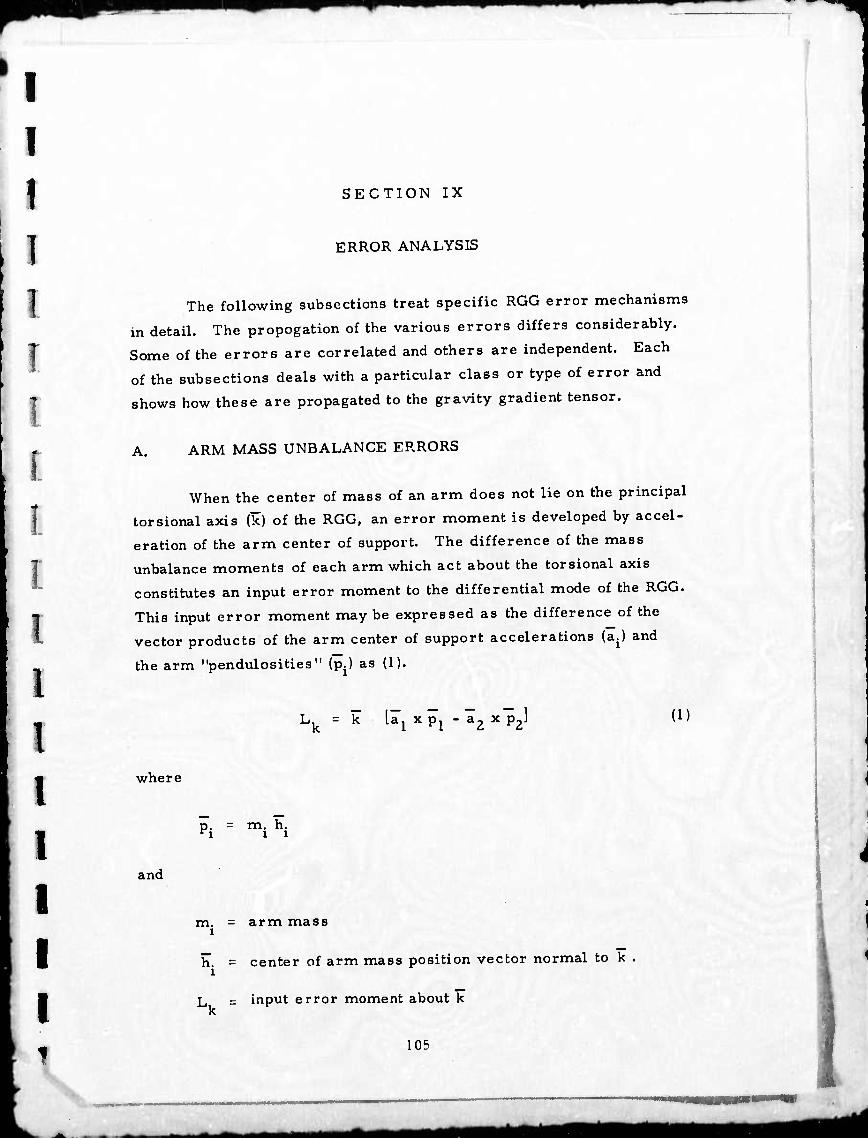
I I
SECTION IX
1 I T I f I I
ERROR ANALYSIS
The following subsections treat specific RGG error mechanisms
in detail. The propogation of the various errors differs considerably.
Some of the errors are correlated and others are independent. Each
of the subsections deals with a particular class or type of error and
shows how these are propagated to the gravity gradient tensor.
A. ARM MASS UNBALANCE ERRORS
When the center of mass of an arm does not lie on the principal
torsional axis (k) of the RGG, an error moment is developed by accel-
eration of the arm center of support. The difference of the mass
unbalance moments of each arm which act about the torsional axis
constitutes an input error moment to the differential mode of the RGG.
This input error moment may be expressed as the difference of the
vector products of the arm center of support accelerations (a^ and
the arm "pendulosities" (p^ as (1).
Lk = k al x Pi " a2 x p2 (1)
where
Pi m. h.
i i
and
m. i
arm mass
h. = center of arm mass position vector normal to k
L = input error moment about k
105
t*m «MflM *M MMHMI

SECTION IX
The error moment of (1) contains two types of mass unbalance
errors, "differential arm ma^s unbalance" and "axial arm mass
unbalance. " This error decomposition is illustrated in (2) and (3).
Ld = k- faox(Pi -PzH
A r k • [ Aa x (pj + p2)]
(2)
(3)
where
a. = a + Aa 1 o
a, = a - Aa 2 o
The average acceleration (a ) of the arm structure is taken at a point
on the torsional axis midway between the arm mass centers, and the
differential arm acceleration (Aa) becomes a function of the axial mass
center separation (H) along the torsional ^xis as defined by (4).
2Aa = uxT+[wx(wxi)] (4)
The difference and sum of the arm "pendulosities" that appear in (2)
and (3) arc defined, for analytical convenience, as the "differential
arm mass unbalance" and the "axial arm mass unbalance" by (5) and (6).
Pd = (Pi "" P2)
Pa = I (Pi + P2)
Substitution of (5) and (6) into (2) and (3) yields the two types of arm
mass unbalance error moments as (7) and (8).
(5)
(6)
Ld = k' [aoxPdl
106
(7)
1 1
!
"!
1 1
1
i
i
/

I I ]
1 r. r
i i: [ t
i i i i
SECTION IX
L = k * [2Aa x pi a ra (8)
Observe that the mass unbalance vectors, pd and pa, are both normal
to the torsional axis (k). For convenience in error evaluation, expan-
sions of the differential arm mass unbalance input error moment of (7)
in both the rotor reference frame (TjTö and the stator reference frame
(xyz) are presented as (9) and (10).
d rdj j^di
a PJ x^dy avPd3
(9)
(10)
The rotor-referenced mass unbalances, (pd^Pd:) are constants, and
the s'-ator-referenced mass unbalances, (pdv.PdJ are periodic functions x y of the rotor spin frequency (cos).
Similarly, expansion of the axial arm mass ".nbalance input
error moment of (8), employing (4), yields (11) and (12) in rotor and
stator reference frames, respectively.
La = *paiK " Tk1 +£Paj[cl'j + wia,k]
La = W^x " WyU,zl +£Pay[d,y + Wxwzl
(11)
(12)
The input error moments to the RGG signal process in a narrow
frequency band centered at twice the spin frequency (Zug) will propa-
gate to output gravity gradient measurement errors. This property
of the RGG signal process infers a particular spectral sensitivity to
the mass unbalance driving functions. For example, the differential
arm mass unbalance error is sensitive to the second spin harmonic of
the rotor-referenced accelerations (a^ a.) and to the fundamental and
third spin harmonic of the stator-referenced accelerations (ax, a ).
107
MM

V ^m
SECTION IX
These same statements apply to the angular velocity and acceleration
driving functions of the axial mass unbalance error functions of (11)
and (12).
Consideration of the different spectral properties of the error
driving functions in both the rotor and stator reference frames may
seem an unnecessary complexity at this point. However, the added
complexity here provides a flexibility in the evaluation of the errors
later on since both rotor-referenced and stator-referenced specifica-
tions of the driving functions may be treated directly without the
necessity of coordinate conversion.
In order to evaluate the RGG arm mass unbalance errors, con-
sideration must be given to the various excitation sources. There are
four potential excitation sources, the snia bearing, the spin motor,
RGG rotor mass unbalance, and the vibration-isolation system (VIALS).
Of the first two excitation sources, only the spin bearing is considered
significant. Of the latter two excitation sources, the VIALS is the most
significant. The main result of RGG rotor mass unbalance is a small
bias (less than 0. 1 EU) with an uncertainty less than 0.01 EU. These
figures are predicated on a rotor unbalance of approximately 2
0.03 gm-cm, a stable platform inertia of approximately 2 #-ft-sec ,
and an offset of the RGG mass center from the stable platform axes of
approximately 10 inches.
Spin bearing excitations of the arm mass unbalance error
mechanism contain both coherent and random components which lead
to bias and random errors, respectively. The initial bias errors are
compensated by the RGG-system initialization process, and the bias
uncertainty thereafter contributes to the output error variance. The
VIALS excitations of the arm mass unbalance error mechanisms are
assumed to be random-only, since the RGG rotor mass unbalance
excitations are considered separately.
In order to evaluate the output errors which result from random
excitations of the arm mass unbalance error mechanisms, it is con-
venient to form the power spectra of the resultant error moments.
These power spectra are then transformed by the RGG signal process
108
1 i
B !
I
0 i
■i
1!
f]
B I
/

I I 1 1 I I I r r.
i i
i i i
SECTION IX
to form the resultant power spectra of the output errors in each RGG
channel. The error variances are then obtained by integration of the
output error spectra. The basis for performing these operations is
documented in Semiannual Technical Report No. 1 and will not be
repeated here. In Technical Report No. I, it was demonstrated that
when the accelerations on each axis of the RGG stator reference frame
(xyz) are assumed to be statistically independent and to have equal
power spectra at the spin frequency and its third harmonic, the
"differential arm mass unbalance" error variances of each RGG channel
are equal and of magnitude stated in (13), where the power spectral
magnitudes, S (f), are the "two-sided" values of a single axis, and
Af is the equivalent bandwidth of the RGG signal process.
2 2 a = cr
c s nc 2r
S (f ) +S (3f ) a s a s
Af (13)
By a sim^ar process, the "axial arm mass unbalance" error variances
of each RGG channel are obtained to first order as (14) since the prod-
ucts of the angular velocities in (12) are small compared to the angular
acceleration terms in the frequency regions of the spin and third
harmonic.
= cr nc
2r
S.(f ) u s s.(3f ; Af (14)
When the output error variances of each RGG in a system of
three are equal and the inter-instrument error correlations are zero
(uncorrelated), the standard deviations of the gravity gradient tensor
errors are given by (15) for the trace elements and by (16) for the
cross-elements.
yz 11
<r.. = —cr ij 2 8
(15)
(16)
4
109
*m

SECTION IX
Thus, the tensor element standard errors due to differential and axial
arm mass unbalance are given as (17), (18), (19), and (20).
ii
/2 3
Pdf nc ^W + Sa^VK (17)
i]
Pdg
nc f[Sa(V+Sa(3f.)lA£e (18)
ii
/2 3 Lie
Pa^ , /[S. (f ) +s. ■y/l w' s' w (3fg)]Afe (19)
lj Pa^ ^J^S.(f8)+S.(3f8)]Afe (20)
The error coefficients in (17) through (20) are estimated on the
basis of the following parameters:
_4 p, =2x10 gm-cm
-3 p =4x10 gm-cm
4 2 HC = 3.066x10 gm-cm
i =2.16 cm
g = 980 cm/sec
[pdg/nC] = 6390 EU/g
[p IhC] * 282 EU-sec 3.
no
(21)
(22)
1 1
1
"i
"i
1 1 1 I
B i
i
i Q
7
^^mamm^m*

I I I 1 I \
I I [ I.
c t I I I I I
SECTION IX
The estimated two-sided spectral values of acceleration due to VIALS
at the spin and its third harmonic are stated in (23) and (24).
S (f ) + S (3f ) ^ 26.8 x 10"10 g2/H2 a s a s a
S.(f)+S.(3f) a 4.84 x 10"R (rad{8ec ) oj s co s' Hz
(23)
(24)
Substitution of the appropriate values in (21) through (24) into
(17) through (20) (for Afe = 0.05 Hz) yields the VIALS-induced arm
mass unbalance standard errors given in (25) through (28).
cr.. ii d
a 0.035 EU
d ä 0.037 EU
11 a
s 0.007 EU
0".. a
a 0.007 EU
(25)
(26)
(27)
(28)
The arm mass unbalance errors attributable to the spin bearing
fall into three categories: (1) bias, (2) bias change, and (3) random.
The bias errors are the result of coherent accelerations at the spin
frequency and/or its harmonics. To the extent that these bias-type
errors do not change after the system initialization process, they do
not contribute to errors of the operating syetem. The bias-type errors
change after initialization for two reasons: (1) the coherent vibrations
of the spin bearing change and/or (2) the RGG mass unbalance coeffi-
cients change.
HI
^rfa tm

SECTION IX
The maximum bias errors as limited by the spin bearing
specification of 10"4g are given by (29) and (30) wherein the bias out-
puts of two RGG's are assumed to add in the worst way
M.. 11
M..
max (!)(¥) do"4) 0.426 EU
max ■ (i)(¥) »«• l) s 0.320 EU
(29)
(30)
The bias variations are assumed to be statistically independent due to
the spin bearing and to RGG error coefficient changes after initializa-
tion. These bias variations contribute to the standard error as
described by (31) and (32).
ii BIAS -mJ' 2 t-V-v a . i (31)
Pd
(T. .
BIAS -mii-y^*-4* (32)
where
a = spin bearing coherent acceleration variance
0", = RGG error coefficient variance d
Evaluation of (31) and (32) for the specified values of o^ = 10 g and
a, = 2/3 x 10"4 gm-cm yields the bias error standard deviations d
given by (33) and (34).
112
n ö D
0 "I 1
1 :1 '\
'!
B <1
Ö
i 1
i A

I
I I 1 !
I r i r.
i
i i i i i
SECTION IX
or.. 11 BIAS
= 3020 X/fl0"10) +(^)(10"8) = 0-105EU (33)
a.. 9 BIAS 3195 WAo-10U(i)flO-8j =0.111EU ( 34)
Th« standard errors due to random accelerations of the spin bearing
are similar in form to (17) and (18) as stated by (35) and (36) wherein
these equations are re-written in terms of the spin bearing acceleration
power at the spin second harmonic.
ii = 4 (^V2^2^^ (35)
1J mj 2[Sa(2fs)] Afe (36)
5 v2 For a specified single-axis random acceleration power of (10 g) in
the effective band around the spin second harmonic, the standard errors
are stated as (37) and (38).
(T. . 11
(T..
63^0
6390
JZ x 10"5 S 0.030 EU
x 10"5 a 0.032 EU
(37)
(38)
A summary of the standard errors due to differential arm mass
unbalance is given in Table IX-1.
113
•^^^ «MM *m* mmmamm

im
SECTION IX
TABLE IX-1
Differential Arm Mass Unbalance Errors
Error Type ... - EU a.. - EU
Bias Uncertainty (la)
Bearing Random
VIAT«S Random
0.105
0.030
0.035
O.lli
0.032
0.037
T830
The axial mass unbalance errors attributable to the spin bearing
may be examined in an analogous manner. The maximum bias error -2 2 as limi .;d by the spin bearing specification of 10 ' rad/sec for
deterministic transverse angular accelerations are stated by (39) and
(40).
i
i
i 1 ")
M.. ii max (i)g)H — (39)
'1
M. Ij max = imn 1.41 EU (40)
The bias variations are assumed to be statistically independent due to
the spin bearing and due to RGG error coefficient changes. The
standard errors which result from these uncertainties are described
by (41) and (42).
B 1
<T.. 11 BIAS ■#&V^(%)'H
114
(41)
3
1
■ ■ - —

rr T I I
SECTION IX
a.. ij BIAS m^^mn
where
(42)
or. = Spin bearing coherent angular acceleration variance
i.
i i i i
cr = RGG error coefficient variance Pa
-3 2 Evaluation of (41) and (42) for the specified values of o". =10 rad/sec -4 w
and o-p = 2/3 x 10 gm-cm yields the bias error standard deviations
of (43) and (44).
ii BIAS 4 <-. ^fPMfff a 0.133 EU (43)
CT..
BIAS = (i) H V (io"3)2+S7s o-i41 EU ,44)
The standard errors due to random angular accelerations of the spin
bearing are expressed similarly to (35) and (36) in terms of total
angular acceleration power on a single axis by (45) and (46).
ii {4m) v^r At. (45)
K = (z) y^c^ 2[S-(2f )] Af 1 « s/J e
(46)
115
tamm
mmmmaäimtk mmtmBmmam
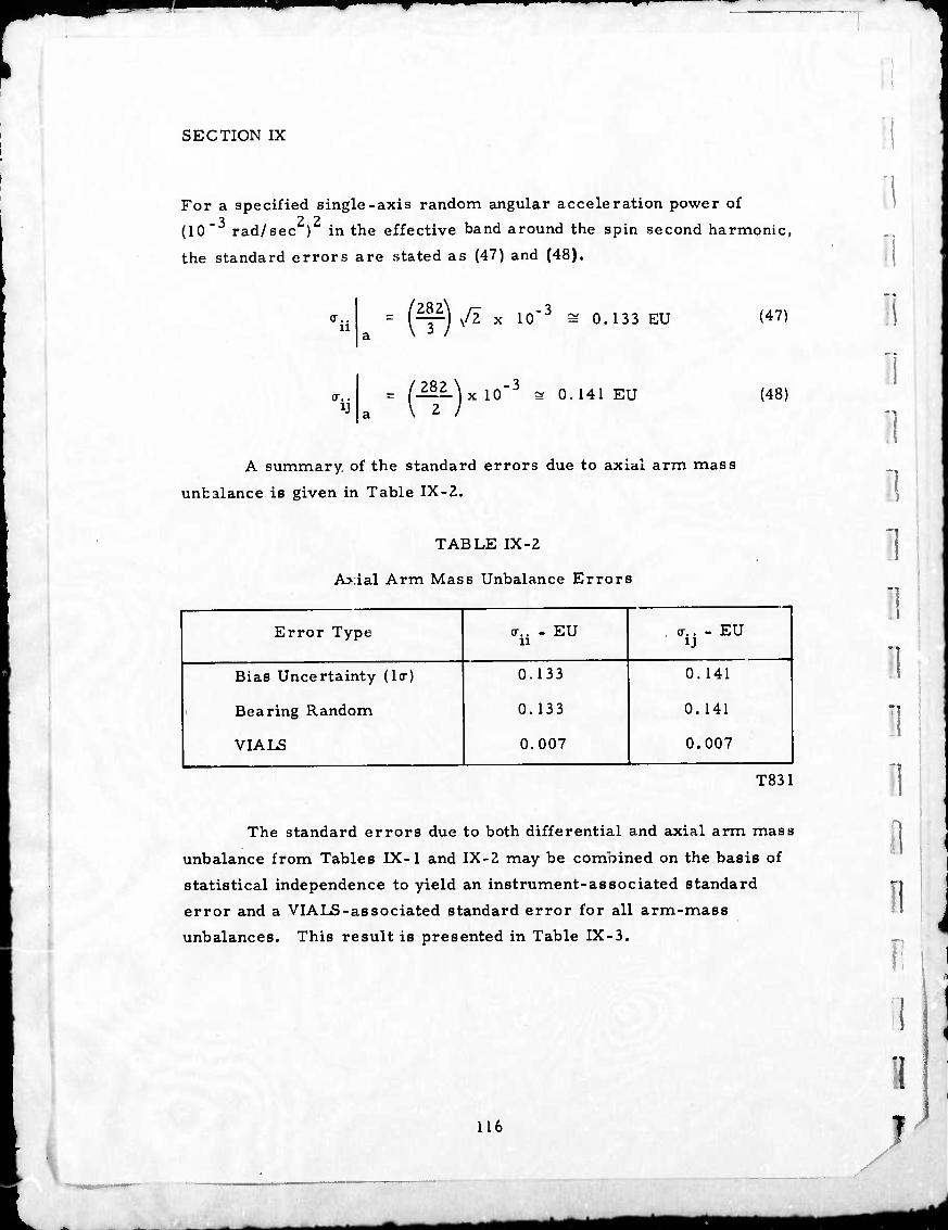
SECTION IX
For a specified single-axis random angular acceleration power of
(10 rad/sec ) in the effective band around th(
the standard errors are stated as (47) and (48).
o 22 (10 rad/sec ) in the effective band around the spin second harmonic,
ii
0". . ij
(¥) ^ « 10 = 0.133 EU
-if) x 10 ^ 0.141 EU
(47)
(48)
A summary of the standard errors due to axial arm mass
unbalance is given in Table IX-2.
TABLE IX-2
Axial Arm Mass Unbalance Errors
Error Type (r.. - EU ii
(T.. - EU
Bias Uncertainty (la)
Bearing Random
VIALS
0.133
0.133
0.007
0.141
0.141
0.007
T831
The standard errors due to both differential and axial arm mass
unbalance from Tables IX-1 and IX-2 may be combined on the basis of
statistical independence to yield an instrument-associated standard
error and a VIALS-associated standard error for all arm-mass
unbalances. This result is presented in Table IX-3.
116
Ö
i
B
/
"i i
1
1
1
1
B fl
I
1 /

I I 1 1 I I I [
r F.
SECTION IX
TABLE IX-3,
Arm Mass Unbalance Error Summary
Error Source ... - EU ... - EU
RGG Instruments
V1AT.S
0.218
0.036
0.231
0.038
T832
B. PHASE ERROR PROPAGATION IN THE ROTATING GRAVITY GRADIOMETER
In this section the phase error sensitivity equations are first
derived. The gradient tensor error is then evaluated for the various
contributing effects.
1. Phase Error Propagation Derivations
Phase errors in the RGG signal process are similar to coor-
dinate misalignments in that they create effective rotations of the
"signal vector" at the particular locations in the signal process where
they occur. For the purposes of system error analysis, these phase
errors may be modelled as error functions associated with either the
modulation or demodulation functions of the RGG signal process. The
modulation process is implemented by spinning the sensor at nominally
constant speed with respect to the measurement reference frame, and
the demodulation ^f ocess is implemented electronically by phase
sensitive detection. The detection process is referenced to the mea-
sured relative position of the sensor with respect to the measurement
reference frame. This method of detection provides a certain amount
of correlation between the modulation and demodulation phase errors ,
and a resultant net reduction in the total effective phase error of the
117
•A ^mk

SECTION IX
RGG signal process. In addition, as part of the initial alignment of
the system, the detection phase reference must be adjusted to match
the initial phase shift (^(o)) of the signal process between the spatially
modulated signal and the input to the demodulation process. Changes
of the phase shift (A^) in this part of the signal process after initial
alignment are considered to be part of the net phase error of the total
signal process.
In order to develop a phase error model for the RGG signal
process, it is necessary to examine the modulation, carrier filter,
and demodulation functions in greater detail. The spatially modulated
input gravity gradient signal ( H ) may be expressed in terms of the
instantaneous angular position, o(t), of the sensor with respect to the
stator reference frame (xyz) for a (z) spin axis as (1).
(r yy
r ) cos 2 a(i) + 2 r sin 2 a{t) xx xy
(1)
The instantaneous angular position, o(t), of the sensor may be modelled
in terms of the constant reference speed command, w . to the speed
control servo and a modulation phase error function, <t)(t), as (2).
a(t) = ta>Rt + <t)(t) (2)
Note that the modulation phase error, <t>(t), is identically the position
error of the speed control servo.
The output signal of the carrier filter process, r . may be
expressed in terms of the input signal. P., and the carrier filter
transfer, H.(s), as (3).
T (S) = H^S) r.(S) o 11
(3)
The carrier filter process may be characterized in terms of its phase
shift at the carrier frequency, vjj(t), and its "equivalent envelope trans-
fer function, " H (s). This equivalent envelope transfer function may
be modelled as a low pass filter with a single time constant, T . as in
(4).
118
^m riM*
i
0
'I
I
!
"I I
1 i
i g
/

^
I
1
r r r
SECTION IX
I
H (S) e T S+l
e (4)
The carrier filter output signal (r ) is demodulated by the instantaneous
angular position of the sensor, a(t), as compensated by the initial carrier
phase shift, \\){o), to form the in-phase and quadrature signals which
are then processed by low pass filters, H (S). An equivalent block
diagram of the entire signal process, based on the input signals of (1),
is shown in Fig. IX-1.
2079- 80
I
Fig. IX-1. Equivalent Block Diagram of Signal Process .
The input signals are resolved by the phase error, Zfyit), of the
modulation p/ocess, and the resultant signals are filtered by the
"equivalent envelope transfer function", H (S), of the carrier filter
process. These filtered signals are resolved by the phase error of
the demodulation process, A^-Z^(t), and the resultant signals are
processed by the low pass filters, H (S), to form the in-phase and A A
r
quadrature output signals, V and F .
The phase-induced errors in the output signals are defined as
the difference between the actual output signals and those that would
occur in the absence of phase errors as in (5) and (6).
119

I
SECTION IX
i Ar c = 1c
< 4 4 S - 8
H (S)H (s) rrvv- r^ e o l yy xx
He(s)Ho{S) [zr^]
(5)
(6)
The phase-induced output errors may be expressed to first order by
assuming the gravity gradient signals. ryy-T^ and Zr^, to be
constant and the phase errors to be very small angles. Substitution of
(4) into (5) and (6) and application of these assumptions yields the first
order phase-induced errors as (7) and (8).
(24)) + ^ - (2«)
(240 +Ai|i - (2<|0
(7)
(8)
Rearrangement of (7) and (8) reveals differences in the propagation of
phase errors depending on the error source as shown in (9) and (10).
a K] K'2'] AvjJ
T S e T S + 1 iM)
s[ r - r xx yy ] h'51] A^j
TeS
T S + 1 e
(2«)
(9)
(10)
Phase errors originating in the modulation process (speed control
servo position errors) do not propagate at low frequency. This is the
direct result of the correlation between the modulation and demodula-
tion phase errors associated with the previously described method of
detection. Phase errors associated with the carrier filter process
(Aijj) do propagate at low frequencies and as a result, phase stability
in the carrier filter process is an important design parameter. Note
that the form of both (9) and (10) are identical except for the background
gradient signal parameters which serve as scale factors in these error
equations.
120
I
!
:
l
i
i
i
[i
"i
■|
B
\\
g
J /
MrtH
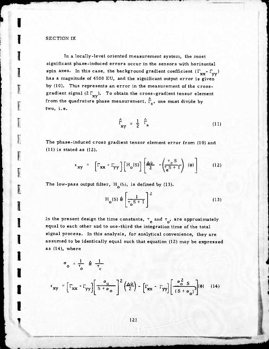
m
I I 1
•
:
SECTION IX
In a locally-level oriented measurement system, the most
significant phase-induced errors occur in the sensors with horizontal
spin axes. In this case, the background gradient coefficient (F - T ) o e. v xx yy has a magnitude of 4500 EU, and the significant output error is given
by (10). This represents an error in the measurement of the cross-
gradient signal (2 T ). To obtain the cross-gradient tensor element
from the quadrature phase measurement, r , one must divide by
two, i.e.
A r xy
= i. r 2 s (11)
I [
The phase-induced cross gradient tensor element error from (10) and
(11) is stated as (12).
xy [rxx-'VyJM 2
The low-pass output filter, H (S), is defined by (13).
tn A Ho(s) £ T S + 1
o
(12)
(13)
In the present design the time constants, T and T , are approximately
equal to each other and to one-third the integration time of the total
signal process. In this analysis, for analytical convenience, they are
assumed to be identically equal such that equation (12) may be expressed
as (14), where
1 1 To " Te
xy [rxx " ryyJ 12
S +« (^H^-ryy] (S + ao)J
(*) (14)
121

SECTION IX
2. Gradient Tensor Error Evaluation
Equation (14) describes the cross-gradient tensor errors which
are the result of misalignments, phase shift variations in the carrier
filter process, and position errors of the speed control servo. All
of these errors, with the exception of the servo position error,
propagate in accordance with the phase uncertainty parameter, (Ai^/Z),
in (14). Errors of this type are assumed to change slowly so that no
real benefit is obtained from the filter process acting on (Aty/2)in (14).
Table I contains a summary from other sections of this report of the
estimated standard deviations of the phase uncertainties in this category
(A^/2). All listed sources are assumed to be statistically independent.
TABLE IX-4
Estimated Standard Deviations
Phase Error Source
Sensor Resonant Frequency Variation
Arm to Rotor Alignment Variation
Disk to Case Alignment Variation
Readout Shift
Electronics Including Frequency Reference
Std. Dev. (A4>/2)
6 x 10⁻⁵ rad
1 x 10"5 rad
1x10" rad
1 x 10"5 rad
1 x 10"5 rad
RSS Total of (A«|»/2)
Tensor Element Standard Deviation
6. 3 x 10" rad
0.28 EU
T833 The servo position error (4>), according to (14), propagates in a
limited low frequency band positioned near the filter frequency,
a = 0. 3 rad/sec. Equations (2) and (3) of Section XVI-B describe the o
speed control servo position error responses to torque disturbances
and tachometer measurement noise. The resultant cross-gradient
122
i
1
i
1
i
i
i
f]
i
i
R
I
1
J ■
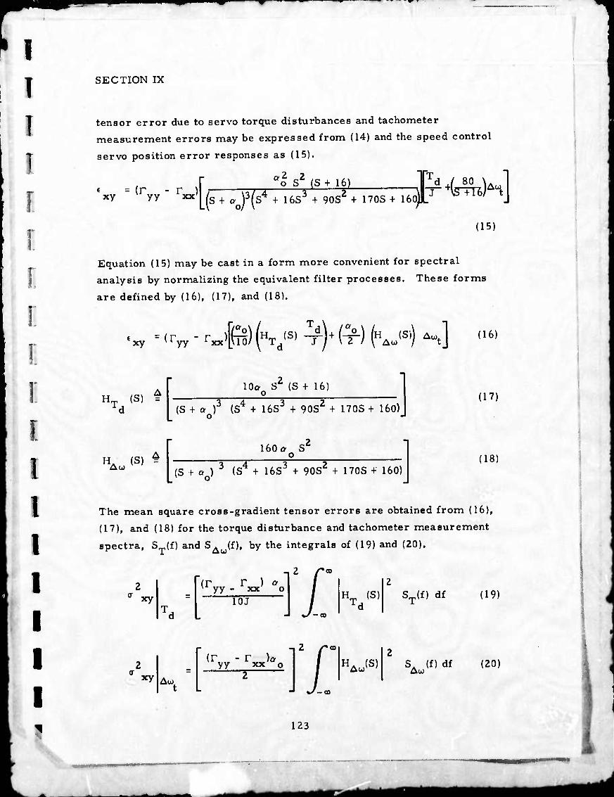
I T I
r [ i
SECTION IX
tensor error due to servo torque disturbances and tachometer
measurement errors may be expressed from (14) and the speed control
servo position error responses as (15).
« = (r - r ) xy yy xx' r ao S2 (S+ 16) "Pd J 80 \. }
(15)
Equation (15) may be cast in a form more convenient for spectral
analysis by normalizing the equivalent filter processes. These forms
are defined by (16), (17), and (18).
« =(r - r ) xy yy xx (?s)(vs,^H^M^] (16)
HT (S) = ^d
10a S2 (S + 16) o
(S + o )3 (S4 + 16S3 + 90S2 + 170S + 160) o
(17)
H. (S) Aw
160 a S o
(S f o ) 3 (S4 + 16S3 + 90S2 + 170S + 160) o
(18)
The mean square cross-gradient tensor errors are obtained from (16),
(17), and (18) for the torque disturbance and tachometer measurement
spectra, ST(f) and SAw(f), by the integrals of (19) and (20).
xy
xy Aw
]2 r* I I w L r* / U I "A
ST(f) df
S. (f) df Aw
(19)
(20)
123
mm
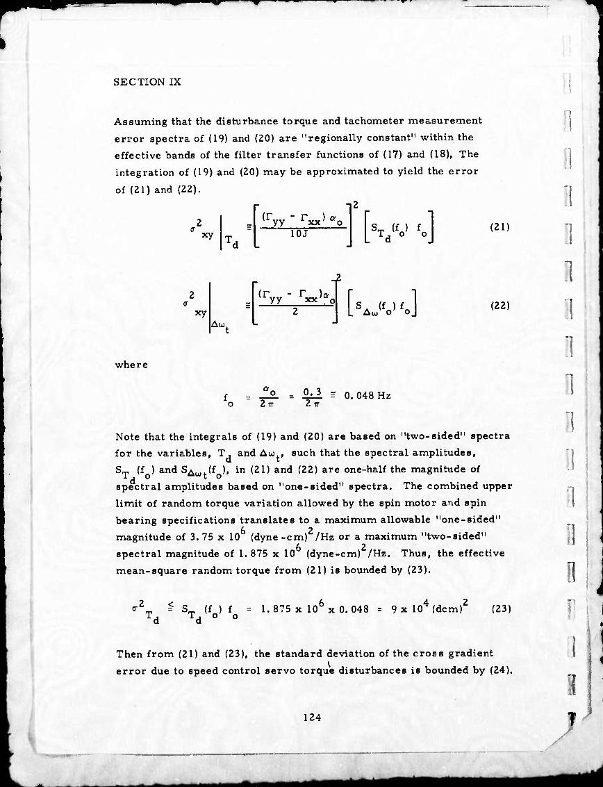
"■■
SECTION IX
Assuming that the disturbance torque and tachometer measurement
error spectra of (19) and (20) are "regionally constant" within the
effective bands of the filter transfer functions of (17) and (18), The
integration of (19) and (20) may be approximated to yield the error
of (21) and (22).
I2
(r. xy
yy r ) a xx' o 10J [v-1 f J
xy AUJ,
(r, yy xx'"o S A (f ) f j L Aw o' oj
where
"o 2TT
£il = 0.048 Hz 2TT
(21)
(22)
!
I !
1 i
1 i
Note that the integrals of (19) and (20) are based on "two-sided" spectra
for the variables, T, and Au., such that the spectral amplitudes, d t
S- (f ) and SAu,.(f ), in (21) and (22) are one-half the magnitude of
spectral amplitudes based on "one-sided" spectra. The combined upper
limit of random torque variation allowed by the spin motor and spin
bearing specifications translates to a maximum allowable "one-sided"
magnitude of 3. 75 x 10 (dyne -cm) /Hz or a maximum "two-sided" L 2
spectral magnitude of 1.875 x 10 (dyne-cm) /Hz. Thus, the effective
mean-square random torque from (21) is bounded by (23).
cr2_ ^ S_ (f ) f = 1.875 x 106 x 0.048 = 9 x 10⁴ (dem)2 (23) Td Td 0 0
Then from (21) and (23), the standard deviation of the cross gradient
error due to speed control servo torque disturbances is bounded by (24).
124
11 v
1 I
r
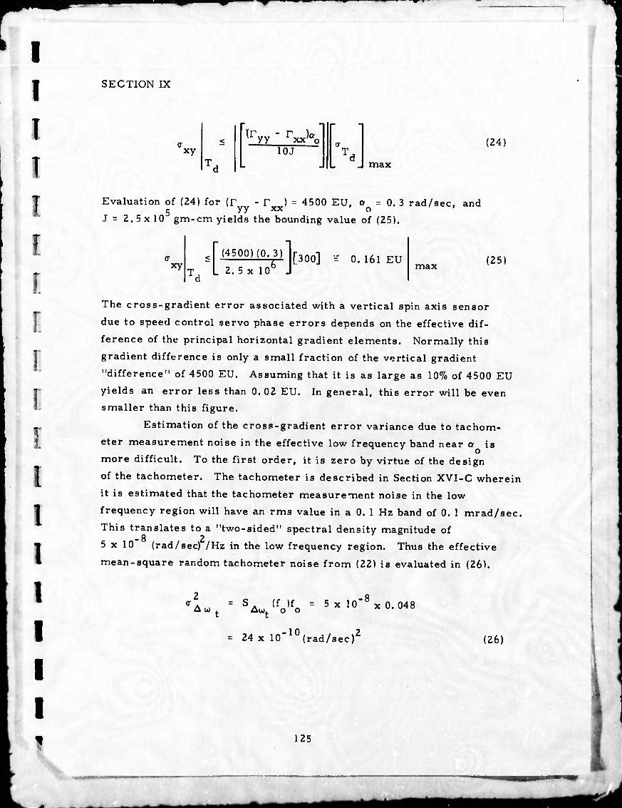
SECTION IX
I
xy
\r yy rxx)oo 10J
(24)
max
Evaluation of (24) for (r - T ) = 4500 EU, o = 0. 3 rad/sec, and c yy ^^ o
J = 2.5x10 gm-cm yields the bounding value of (25).
[300] = 0. 161 EU xy
r(4500)(0.3) I "L 2. 5x 10⁶ J max (25)
The cross-gradient error associated with a vertical spin axis sensor
due to speed control servo phase errors depends on the effective dif-
ference of the principal horizontal gradient elements. Normally this
gradient difference is only a small fraction of the vertical gradient
"difference" of 4500 EU, Assuming that it is as large as 10% of 4500 EU
yields an error less than 0.02 EU. In general, this error will be even
smaller than this figure.
Estimation of the cross-gradient error variance due to tachom-
eter measurement noise in the effective low frequency band near o is
more difficult. To the first order, it is zero by virtue of the design
of the tachometer. The tachometer is described in Section XVI-C wherein
it is estimated that the tachometer measurement noise in the low
frequency region will have an rms value in a 0. 1 Hz band of 0. 1 mrad/sec.
This translates to a "two-sided" spectral density magnitude of - 8 2
5x10 (rad/sec) /Hz in the low frequency region. Thus the effective
mean-square random tachometer noise from (22) is evaluated in (26).
A UJ Au). o o
10 24 x 10 (rad/sec)
5 x 10"8 x 0.048
2 (26)
125
*mt

wmm
SECTION IX
Then, from (22) and (26), the standard deviation of the cross-gradient
error due to low frequency tachometer noise is evaluated in (27).
xy ALO
__ |-(4500)(0.3)] ^g^o-B) 0.033 EU (27)
The total cross-gradient standard deviation due to all phase
errors in the horizontal spin axis sensors may be computed from the
values given in Table I and in equations (25) and (27) as shown in (28).
xy All Phase Errors = V(0. 28)2 + (0. 161)2 + (0.033)2 = 0. 325 EU
(28)
Similarly, for the vertical spin axis sensor, the cross-gradient
standard deviation due to all sources of phase error will be less than
0. 03 EU if the principal horizontal gradient difference is less than
400 EU.
C. TRANSDUCER LOAD STUDY - THERMAL NOISE
Previous analyses of thermal noise employed a single equivalent
dissipative element in the model of the electromechanical signal sensing
and transducing process. A more accurate representation of this
process requires at least two dissipative elements: one to represent
the mechanical losses and one to represent the electrical losses asso-
ciated with the signal transducing process. The intent of this study is
to examine the relation between thermal noisr on the gravity gradient
tensor elements and the "effective Q" of the signal sensing and transducing
process when 'he total signal process is constrained to have a fixed
integration time of 10 sec in terms of signal transmission. The results
of the study for transducer load resistances in the range 2. 86 to
28. 6 megohms indicate a small increase in thermal noise (about 5%)
126
i
i
"!
1
1 1
1
I
H [I
i
i 8 r
i
1
s

I 1 ] i [ r.
i:
SECTION IX
with respect to the no-load case for the same "effective Q" of the signal
sensing and transducing process.
1. Sensing and Transducing Equivalent Circuit
An equivalent circuit of the signal sensing and transducing
process is shown in Fig. IX-2. The resistors, R, and R , represent
the mechanical damping and transducer loading, respectively. The
reactive elements, L. and C., represent the equivalent inertia and
elasticity of the mechanical system, and C ia the electrical capacity
of the transducer.
For convenience, the electrical equivalents of the mechanical
components have been transformed to the output side of the equivalent
circuit in this figure. The mechanical impedances have been divided
by N and the primary voltages divided by N, where N is the system
transformation ratio discussed in Section XIV-A. Therefore, except
for C , R , andw , the magnitudes of the various elements are not the
same as in other sections of this report. The noise calculations are in
normal units. The voltage generators, e. and e?, represent the white
noise sources associated with R. and R0, and E represents the input
gravity gradient signal at scale factor K as in eq. (1). s
E8 A ^(zr.j) (i)
.i outpu^signal (e ) of Fig. IX-2 is processed by the
remainder ' the RGG signal process to yield the gravity gradient tensor
elements. This latter process must be selected according to the param-
eters in Fig. IX-2 so that the total process acting on the signal (2 F--)
satisfies the 10-sec integration time requirement. To select this
process, we state the input-output signal transfer as eq. (2).
127
*mimm

207S-M
c. 7 s
> (
: Li ;
R0:
r" sCo
•o
G)6* 1
Fig. IX-2. Equivalent Circuit of Signal Sensing and Transducing Process.
I
i
1 I
1
i
128
I
R ■
I 1
r *mak

I
I I 1 1 I I B [
SECTION IX
where
H^s) ICT+C \ 1 ol
2 s o
s3+ (Vi)sH o
a a\s + a ß. o 1/ o 1
"o » R C o o
•l« Ri
^# i
Lici
2 . i (ci+c0\ the undamped
natural frequency.
(2)
The signal transfer, Hj (s), may be restated as eq. (3) in factored
form
1 u2S lci+c0r°
H.(8) =
o
(3)
In (3), by definition, ß is the resonant frequency of signal
transmission, and Q is the "effective Q" of the signal sensing and
transducing system. The equivalent carrier filter process, H^s), for
the remainder of the signal process to either the RGG in-phase or
quadrature outputs, F and T , is stated as (4).
1 129

v ■■■
1 SECTION IX
H (s) o
^^o' K
ßoV4+ßo Q w2
o o
(4)
The parameter, Q2, of eq. (4) must be selected to satisfy the
integration time requirement.
2. Thermal Noise Evaluation
The thermal noise variances on each RGG output channel, tr2
and <Tg , due to Rj are computed as in (5).
T2 = ,2 'l 81
00
ZkTR. I H1(s)Ho{s) df (5)
2 2 The variances, v^ and ag , due to R0 are computed as in (6).
o-2 = o-2 =2 kTR C2 82 0 .
00
I H?(8)H (8) i. o df (6)
I
1 1
"1
Q
!
I
where
H2(8)
(s+.o)(s24 s+P2)
(7)
The total channel variance8 are simply the sums of the individual
variances due to the statistical independence of e. and e .
2 _ 2 2 (T -0" +0"
c c1 c2
130
(8)
!
11 i
II
A ^^^m ^mmmtämlM

I 1 !
I
r
SECTION IX
2 2 2 (T = (T + (T
Sl S2 (9)
The gravity gradient tensor element standard deviations for a system of
three orthogonal sensors are stated as eq. (10) for the trace elements
and as (11) for the cross-gradient elements.
ii
ij
3 c
1 2 s
(10)
(11)
The noise integrals of (5) and (6) were evaluated for a fixed set
iive elen
elements, i. e.,
of reactive elements, (L., C,, C ), and a variable set of dissipative
125 kft < R. < 1.25 Mf2
2. 86 Mfi < R £ 28. 6 Mn
Cj = 41pF
C = 3490 pF o r
w2 = (220)2 rad/sec o
This set gave a range of mechanical quality factor, Q , from 88 to 880
and a range of effective quality factor, Q ff. from 62 to 589.where
m WolRl (C11 + V
131
^ma^m
- *M
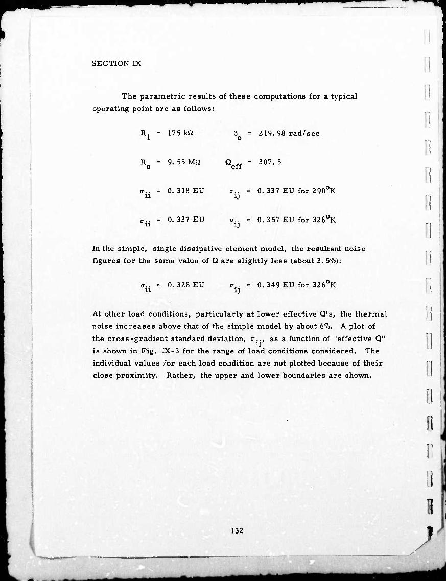
^wwpvi
SECTION IX
The parametric results of these computations for a typical
operating point are as follows:
Rj = 175 kn ß = 219. 98 rad/sec o
i
1
R = 9. 55 Mn o Q „ = 307. 5
eff
o-.. = 0.318 EU o-.. = 0. 337 EU for 290UK
o-.. = 0. 337 EU o-,. = 0.3 57 EU for 326UK
In the simple, single dissipative element model, the resultant noise
figures for the same value of Q are slightly less (about 2. 5%):
o-.. = 0. 328 EU ii ij
0. 349 EU for 3260K
At other load conditions, particularly at lower effective Q's, the thermal
noise increases above that of ^he simple model by about 6%. A plot of
the cross-gradient standard deviation, cr.., as a function of "effective Q"
is shown in Fig. .[X-3 for the range of load conditions considered. The
individual values for each load condition are not plotted because of their
close proximity. Rather, the upper and lower boundaries are ohown.
'I
I
n
W
f
132
■|
J

SECTION IX
2 2 2 (T =0" +0"
Sl S2 (9)
The gravity gradient tensor element standard deviations for a system of
three orthogonal sensors are stated as eq. (10) for the trace elements
and as (11) for the cross-gradient elements.
ii
iJ
3 c
1 2 s
(10)
(11)
The noise integrals of (5) and (6) were evaluated for a fixed set
tive elen
elements, i. e. ,
of reactive elements, (L., C., C ), and a variable set of dissipative
125 kfl < Rj < 1.25 un
2. 86 Mfi < R 5 28. 6 MO o
Cl = 41 pF
C = 3490 pF
w2 = (220)2 rad/sec o
This set gave a range of mechanical quality factor, Q , from 88 to 880 m and a range of effective quality factor, Q ,., from 62 to 589.where
Q m u R. IC, C J , 1 \ 1 o/
131

SECTION IX
The parametric results of these computations for a typical
operating point are as follows:
Rj = 175 kn 219. 98 rad/sec
R = 9. 55 Mß Q « = 307. 5 o eff
o-.. = 0.318 EU o-.. = 0.337 EU for 290"K ü ij
o-.. = 0.337 EU o-.. = 0.3 57 EU for 326UK ii ij
In the simple, single dissipative element model, the resultant noise
figures for the same value of Q are slightly less (about 2. 5%):
o-.. = 0. 328 EU ii
0. 349 EU for 3260K
At other load conditions, particularly at lower effective Q's, the thermal
noise increases above that of the simple model by about 6%. A plot of
the cross-gradient standard deviation, o-.., as a function of "effective Q"
is shown in Fig. IX-3 for the range of load conditions considered. The
individual values for each load cordition are not plotted because of their
close proximity. Rather, the upper and lower boundaries are shown.
132
I • j
i i
i
!!
[1
II 11 r ii 8
^
i^tfa *m

I I 1 I i
'{.
r o
r
i !
I I I i
0.8
3 ui
§0.6 K
e 0.4
i 0.2
cors-ti
UPPER BOUND FOR FINITE TRANSDUCER LOAD RESISTANCE IN RAN<>E (2.86M TO 28.6 M)
LOWER BOUND FOR INFINITE TRANSDUCER LOAD RESISTANCE
100 200 300 400 SOO EFFECTIVE "o"
Fig. IX-3. Standard Deviation Cross-Gradient Thermal Noise (a-jj) Versus Effective Q. (These Curves were Plotted for 290oK. For 3260K, Multiply o1d by 1.06.)
133

SECTION IX
D. ROTATIONAL FIELD ERRORb
In Section III-B-2 of Technical Report No. I, the equivalent
input power spectra of the rotational field errors to each RGG channel
were derived and presented as eqs. (30) and (31), and the bias errors
were presented in eqs . (9) and (10). When a system of three mutually
orthogonal RGG's are subjected to the same inertial angular velocity,
the resultant rotational field errors of each instrument are correlated.
When this is the case, this correlation must be considered in the
calculation of the rotational field trace element errors of the gravity
gradient tensor. Since only one RGG is employed in the measurement
of each cross-gradient tensor element, inter-instrument error corre-
lation is not a consideration in the determination of the cross-gradient
tensor errors. For common inertial angular velocity excitation, the equivalent
input rotational field error spectra to the RGG signal process for
calculation of the trace element errors may be derived using the
method employed in Technical Report No. 1 to obtain the equivalent
input error spectra to each RGG channel. As an example, the complete
input rotational field error spectrum for the XX trace element error
is presented in (1) for the correlated case.
SXX. (f)
in | [sx(f) * sx(f) ] + I [Sy(£) * Sy(f) + S^{f) * Sz(f)]
" I [Sxy(f) * Sxy(f) + Syx(f) * V£) ]
- I [Sxz^ * Sxz<f) + Szx<f) * Szx (f)]
H|[Syz(f)*Vf)+Vf)*Vf)]
+ I [4Mx Sx(f) + My Sy(f) + Mz Sz(f)]
I.
1
i
I i !
1 i
i
;i 134
/»
--
UMfll MM mmmmmmm

I
tOTö-«l
0.8
uJ
er o tr UJ
oc o tn
0.6
0.4
UJ
5 I B (O 0.2 M 8 o
UPPER BOUND FOR FINITE TRANSDUCER LOAD RESISTANCE IN RANGE (2.86M TO 28,6 M)
LOWER BOUND FOR INFINITE TRANSDUCER LOAD RESISTANCE
100 200 300 400 900 EFFECTIVE "o"
Fig. IX-3. Standard Deviation Cross-Gradient Thermal Noise (o<.j) Versus Effective Q. (These Curves were Plotted for 290oK. For 3260K, Multiply aid by 1.06.)
133
M^^te.

SECTION IX
D. ROTATIONAL FIELD ERRORS
In Section III-B-2 of Technical Report No. 1, the equivalent
input power spectra of the rotational field errors to each RGG channel
were derived and presented as eqs. (30) and (31), and the bias errors
were presented in eqs . (9) and (10). When a system of three mutually
orthogonal RGG's are subjected to the same inertial angular velocity,
the resultant rotational field errors of each instrument are correlated.
When this is the case, this correlation must be considered in the
calculation of the rotational field trace element errors of the gravity
gradient tensor. Since only one RGG is employed in the measurement
of each cross-gradient tensor element, inter-instrument error corre-
lation is not a consideration in the determination of the cross-gradient
tensor errors. For common inertial angular velocity excitation, the equivalent
input rotational field error spectra to the RGG signal process for
calculation of the trace element errors may be derived using the
method employed in Technical Report No. 1 to obtain the equivalent
input error spectra to each RGG channel. As an example, the complete
input rotational field error spectrum for the XX trace element error
is presented in (1) for the correlated case.
SXX. (f)
in
8 7 [sx(f)* Sx(f)] + | [sy(f) * Sy(f) + Sz(f) * Sz(f)]
■ I [Sxy(f) * Sxy{f) + Vf) * V£) ]
" | [Sxz<f) * SxzW + Szx<f) * Szx (£)]
+|[Vf)*Vf)+Vf)*V£)]
+ | [4Mx Sx(f) + My Sy(f) + Mz Sz(f)]
• i
I n
i
i i
i I n I
134

■•V
SECTION IX
+ i IM M Is (f) +S (f) ( - 2M M |Sv (f) + S (f) 9 L y z | yzw *y \ x y j xy yx
2M M IS (f) +S (f) X Z ) xzx zx (1)
When the rotational field environment of each RGG is statistically
independent of the others, eq. (30) of Technical Report No. 1 may be
applied to each individual RGG to obtain the error variances of each
RGG channel, and the resultant error variances of pairs of instru-
ments may be combined on the basis of statistical independence to
obtain the gravity gradient trace element error variancee. Self-
induced rotational fields of each RGG, e.g., from each spin bearing,
have inter-instrument statistical independence. On the other hand,
the common angular velocities of the vibration-isolation system
(VIALS) produce inter-instrument correlation, and this requires employ-
ment of input error spectra of the form of eq. (1) to obtain the trace
element variances.
The correlated trace element rotational field bias errors are 2 2 2
stated as (2), (3), and (4), where the «r , a , a are the angular X y Z
rate variances of the common rotational field environment.
M XX
M YY
= H2%-( 2 , a + a
= T L^y " (^ " + ff X Z
)]
)]
(2)
(3)
M ZZ ^N-^'y)] (4)
In the uncorrelated case, the trace element bias errors depend
on the rate variances associated with pairs of RGG's. As an example.
? 135

the uncorrelated XX trace element bias is presented as (5) where
the superscript is used for RGG spin axis identification.
M XX _ i r 2 2iY , i r 2 zi
i L x zJ 3 L x yj (5)
Observe that the rate variances, cr , in each term of (5) are two
different variances; the first is related to the RGG with a Y spin axis,
and the second is related to the RGG with a "Z spin axis.
The cross-gradient bias errors are of the same form for both
uncorrelated and inter-instrument correlated cases as shown in (6),
(7), and (8), where the C^o) are the angular rate covariance functions
evaluated at zero time shift.
M = C (o) XY xy (6) 1
Mv„ = C (o) XZ X2V
M = C (o) YZ yz
(7)
(8)
For the purpose of estimating the rotational field error
variances of the gravity gradient tensor elements, it is convenient
to assume the angular rate cross spectra to be zero for two reasons:
(1) a great simplification of the equivalent input error spectra is
achieved, and (2) at present there is no sound basis for estimation of the
cross spectra. This assumption may be justified by considering that
the basic effect of non-zero angular rate cross spectra is to redistri-
bute the rotational field errors between RGG channels without appre-
ciably altering the total system error for a given angular rate power.
When the cross spectra are zero, eq. (1) reduces to (9) for the
correlated case.
136
1
H
1
D 0
ll "I
J '■ ^*m ^^^ ■■MB

w^
1 1 I [ [ B 1. r. i: r
r. [ i
i i i
i
SECTION IX
SxXin(f) = I [Sx(f) ::C Sx(f) ] + I [Sy(£) * Sy(f) + SZ
{f) * SM
4[4M2S 9 L xx ■ + M2 S (f) + M2 S (f) y y z Z J (9)
In the uncorrelated case, the equivalent input error spectrum of the
XX trace element is just the weighted sum of the error spectra of
the Y and "Z spin axis RGG in-phase channel error spectra as defined
by (10).
sxx.(f) = i [ in
S*(f) + S^(f) J (10)
When the cross spectra are zero, eq. (10) may be expressed (from
eq. (30) of Technical Report No. 1) as (11) wherein the superscript
spin-axis identification is employed.
sxx. <f> in
= | [ Sx(f) * Sx(f) + Sy(f) * Sy(f) ]
I [Sx(f) *Sx(f) ■ Sz(f) *Sz(f)]
l[- - I M2 S..(f) + M2 SJi) j y y X X
l[ M2 Sz(f) + M2 Sx(f) ] (ID
The equivalent input error spectrum of the XY cross-gradient
tensor element for either the correlated or uncorrelated cases is
just the weighted spectrum of eq. (31) in Technical Report No. 1.
When the cross spectra are zero, the equivalent input "^Y cross-gradient
error spectrum is given by (12).
137
ttmmm

V 'W*
SECTION IX
SXY (f) = Sx(f) ♦ S (f) + MZ Sx(f) + M^ S (f) in
(12)
I
I
Ö
For the purposes of error estimation, a further simplification
results when all of the rate spectra and average rates of each axis are
assumed to oe equal to S (f) and M , respectively. When these assump.
tions are applied to (9), (11), and (12), the equivalent input error
spectra of (13), (14), and (15) are the result.
Sii(f)
S..(f) ii
S..(f) 1J
- Ü \s (f) S (f) tit
+ IM2 s (f) 3 GO to
corr
8 1 L w
(f) * S (f) 10
]+ ijf. M- 4M2
9 OJ OJ
uncorr
S (f) * S . OJ
(£)] U J
+ ZU1' S (f) OJ OJ
(13)
(14)
(15)
all
Observe that the correlated case of (13) is a little larger than
the uncorrelated case of (14). The gradient tensor error variances
are estimated by integration of the equivalent output error spectra
obtained from the equivalent filter of the RGG signal process acting on
the appropriate input error spectra as defined by (16) and (17) where
H (s) is the equivalent lowpass filter of the RGG signal process.
ii
ij
■L
■I
H (iZirf) e
S..(f)df ii
(16)
H (jZnf) S..(f)df (17)
138
D 1
1 1
i
1
1
1
'I
1
(1 F
II
11 /
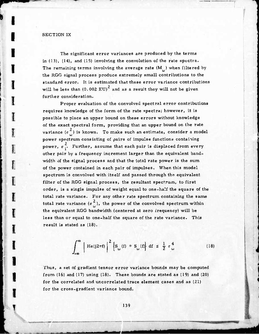
SECTION IX
1 I I
The significant error variances are produced by the terms
in (13), (14), and (15) involving the convolution of the rate spectra.
The remaining terms involving the average rate (M ) when filtered by
the RGG signal process produce extremely small contributions to the
standard error. It is estimated that these error variance contributions
will be less than (0.002 EU) and as a result they will not be given
further consideration.
Proper evaluation of the convolved spectral error contributions
requires knowledge of the form of the rate spectra; however, it is
possible to place an upper bound on these errors without knowledge
of the exact spectral form, providing that an upper bound on the rate
variance (c ) is known. To make such an estimate, consider a model w power spectrum consisting of pairs of impulse functions containing
2 power, a .. Further, assume that each pair is displaced from every
other pair by a frequency increment larger than the equivalent band-
width of the signal process and that the total rate power is the sum
of the power contained in each pair of impulses. When this model
spectrum is convolved with itself and passed through the equivalent
filter of the RGG signal process, the resultant spectrum, to first
order, is a single impulse of weight equal to one-ha'.f the square of the
total rate variance. For any other rate spectrum containing the same
total rate variance (a ), the power of the convolved spectrum within
the equivalent RGG bandwidth (centered at zero frequency) will be
less than or equal to one-half the square of the rate variance. This
result is stated as (18).
f .'-co
He(j2TTf) Is (f) * S (f)) (18)
Thus, a set of gradient tensor error variance bounds may be computed
from (16) and (17) using (18). These bounds are stated as (19) and (20)
for the correlated and uncorrelated trace element cases and as (21)
for the cross-gradient variance bound.
5 139

~T
SECTION IX
2 a .. ii
corr
< 6 9
4 a
(0
2 (T ..
11
uncorr
< 4 9
4 (T
2 11 ij
< 1 2
4
(19)
(20)
(21)
all
Finally, the standard deviation bounds of the rotational field errors
are stated as (22), (23), and (24).
ii
corr
< sff, T
2
ii
uncorr
< 2 3
2
< I
^2
2 a
(22)
(23)
(24)
lall
It is interesting to observe that all of these standard error bounds
are approximately equal.
140
'1
1
I
0
I
"I
1
I
a
ii
H
■n»-™"" —•
- — mm *m*m^mi^mM

SECTION IX
Having developed these standard error bounds, it is a simple
task to evaluate the rotational field error contributions from the various
error sources. First, let us consider the errors induced by the VIALS.
In Section VII, an upper bound on the rate variance of the stable plat-
form was established and is restated in (25).
w VIALS
*( 9. 27 x 10" rad/sec (25)
Substitution of (25) into (22) and (24), yields the VIALS-induced rota-
tional field errors as (26) and (27).
'u <1('-""°-6): x lO7 a 0.070 EU (26)
.. < -(9. 27xlO"M x 109 a 0.061 EU (27)
Transverse angular velocity induced by the spin bearing of each
RGG causes rotational field errors that are statistically independent
between instruments. The spin bearing specification requires that the
transverre angular rates produced by the bearing be limited so that
the induced bias of each instrument channel does not exceed ±4 EU with
a maximum bias uncertainty of 0. 04 EU. In addition, it is required
that the standard error of each channel due to random bearing-induced
rates be limited to 0. 04 EU in each instrument channel. The 0. 04 EU
bound translates to an equivalent rate variance bound of
0. 283 x 10"10 (rad/sec) . The statistical combination of the bias
uncertainty and the random standard error bounds translates to an
equivalent rate variance bound of 0. 4 x 10" (rad/sec) . Using this
141
«a *m*

SECTION IX
rate variance bound in (23) and (24), we obtain the spin bearing-induced
rotational field enors as (28) and (29).
0".. 11 s (|)(o.4x 10"10)/l09) H 0.027 EU (28)
RGG MU
Substitution of this rate variance into (22) and (24) yields standard
errors of approximately 0, 001 EU. It is concluded that RGG rotor
mass unbalance causes negligible rotational field errors.
In summary, only the spin bearing and the VIALS produce
significant rotational field errors. To complete the rotational field
error analysis, consideration must be given to the bias uncertainty of
the VIALS-induced errors. The bias errors are defined by (2), (3),
and (4) and by (6), (7), and (8) for the trace and cross-gradient tensor
elements, respectively. When the previous assumptions of equal and
'
n
ij -(i)(0-4xl0"10)(109) = 0.028 EU (29) I!
I Spin motor-induced rates normal to the spin axis are assumed
to be negligible in comparison to the bearing-induced rates because of
the high bearing stiffness and the small motor forces.
Platform angular rates due to RGG rotor mass unbalance of
(0. 03 gm-cm) produce bias errors to the extent that they remain con-
stant after initialization. It is estimated that the RGG rotor mass-
unbalance induced platform rates on each axis will be less than
3x10 rad/sec and that the amplitudes will be stable to bet.er than
10% of their values. This leads to the rate variance bound defined
by (30).
2
1
D 2(3x 10"6)|o. 3x 10'6) (30)
1 F I a
142 1 ä 1
/
^m*

SECTION IX
independent rate spectra are applied to these bias equations, the
resultant biases are zero. To estimate bias uncertainty, a departure
from the previous assumptions is required. One possibility is to
assume non-stationary statistics for the VIALS-induced angular rates
and then to compute the bias variances on the basis of the variances of 2 2 the rate variances. For this purpose, let the rate variances, or , o- ,
2 x y 0" , be represented by the independent random variables, a, ß, y.
Further, assume that the probability density function of each of these
random variables is of the same form and equal to zero outside of the 2 I positive region zero to cr . Under these conditions, the expected 0 co | max r
value of the bias is zero. This may be demonstrated by substitution
of the random variables, a, ß, Y, into (2) as shown in (31).
M xx = } [2a- p-v] (31)
EtMxx] = \ [2Et*l " EIP1 -EW] (32)
Since the random variables all have the same probability density,
their expected values are equal leading to an expected bias of zero
from (32). The variance of the bias, cr , is defined by (33) when the
random variables are statistically independent.
m = \ [4E[a2] + E[ß2] + E[Y2]] (33)
Since the probability densities are assumed to be the same, (33) may be
expressed as (34).
m T E[*2] (34)
143

SECTION IX
The expectation in (34) is the variance of the rate variance. This
expectation may be calculated on the basis of an assumed probability
density function. For this purpose, let's select arbitrarily the density
shown in Fig. IX-4. The second moment of a is evaluated in (35) for
the density function of Fig. IX-4.
0 i
li
E[a2] / Jo
max ^2 _ , . a pa(a) da C GO
(35) max
From (34) and (35), the resultant variance of the bias is given in (36).
"I
m i'4 3 OJ
(36) max
The standard error is given by (37).
m 1 ^2
V3 CJ (37)
max
An upper bound of the VIALS rate variance was defined by (25). Sub
stitution of this value into (37) yields an estimate of the bias uncertainty
due to VL/iLiS-induced rate errors.
m (9. 27)Z x 10'12 x 109
35 a 0. 050 EU (38)
144
fl n
ß (1 r
I J /
-

*
]
I I i
2075-23
I
I.
2/0^1 MAX
V I MAX
Fig. IX-4. An Assumed Probability Density Function.
145

SECTION IX
A summary of the rotational field errors is given in Table IX-5.
It is recognized that the method of estimating the VIALS-induced bias
uncertainty is quite arbitrary, but it does provide some indication of
the size of this error source based on an upper bound for the angular
rate variance.
TABLE IX-5
Summary of Rotational Field Errors ^
Error Source
Spin bearing total
VIALS random
VIALS bias uncertainty
Total VIALS
ff. -EU 11
0.027
0.070
0.050
o:o86
(r..-EU
0.028
0.061
(0.050)*
0.079
♦Actually this value should be zero for the stated assumptions but the same vllue was used here as was derived for the ^ •^•^bUB
uncertainty, because the stated assumptions are quite arbitrary.
T868
E. SUM-MODE MISMATCH ERRORS
The sum-mode mismatch error nechanism provides an excita-
tion of the RGG differential mode through RGG rotor spin axis accelera-
tions occurring in a narrow frequency band centered at twice the spin
frequency (2(0 ). In Technical Report No. 1. it was demonstrated that
errors of this'type can be represented in terms of an equivalent input
error to tne RGG carrier signal process, which is proportional to the
RGG rotor spin axis disturbance torques in a narrow frequent band
centered at twice the spin frequency as described by (I), wherein "T/
represents the narrowband spin axis disturbance torque. Kp is the
146
i
!
1 1 1
1 11 1 1
i
1
1
B
'I
ü
J /

^
■ I I
11 ill
l
I r
i
i
SECTION IX
sum-mode mismatch factor, n is the arm inertia efficiency, Po is the
nominal sum mode frequency, and J is the total polar inertia of the RGG
rotor.
in
2 ßo
(2u)8)' oj
m (i)
Both deterministic and random excitations of this error mecha-
nism are possible. Deterministic excitations produce bias errors
which may be compensated during RGG system initialization to the
extent that these excitations remain stable. Changes in the bias errors
after initialization and random excitations contribute to the total error
variance. Potential excitation sources are the spin bearing, the spin
motor, the speed control servo, and the vibration-isolation system
(VIALS). It is convenient to analyze the errors of each channel of an indi-
vidual RGG instrument in this case and then to determine the gravity
gradient tensor element standard errors from the individual instrument
errors. The bias errors of each RGG channel will be determined on
the basis of the spin bearing and spin motor specifications and an esti-
mate of the tachometer disturbance through the speed control servo.
When the speed control servo position error is sampled only once per
revolution, no significant torque disturbances at twice the spin frequency
due to sampling noise are anticipated, and the load torque disturbance
from the VIALS is considered to be random only.
The random errors of each channel will be determined on the
basis of (1) bias uncertainiy due to both excitation uncertainty and RGG
error coefficient uncertainty, and (2) random excitations acting on the
nominal RGG error coefficient. The resultant random errors of each
channel will then be converted to gravity gradient tensor standard errors
on the basis of inter-instrument statistical independence.
i
147

SECTION IX
I
The first logical step in the analysis is to establish the bias
errors of each channel. To accomplish this, it is convenient to eval-
uate the RGG error coefficient of (1) for the following parametric
values:
kp = lO-6
1 = 0.86
ß = 128 rad/sec o
2co = 220 rad/sec s 5 2 J = 2. 5 x 10 gm-cm
The resultant error coefficient is evaluated in (2).
= 2.37 x 10 -3 EU dem (2)
The spin bearing specification allows a deterministic disturbance torque
of 1000 dem at twice the spin frequency. Assuming this disturbance
torque to have equal contributions of 707 dem to each RGG channel, the
resultant spin bearing bias is given by (3) from (1) and (2).
1 1 1 B D
"i
1
I
M = M = (2.73 x 10'3)(707) 3 1.68EU c s (3)
Similarly, the specification for each motor allows a deterministic dis-
turbance torque of 500 dem. There are two motors, and the probable
net disturbance torque is 707 dem. Assuming this is distributed equally
in each RGG channel, the resultant spin motor bias is given by (4) from
(1) and (2).
il
M M = (2.73 x 10"J)(500) M 1.19 EU
148
(4)
]
J

BI-
SECTION IX
Finally, it is assumed that the deten ilnistic tachometer signal noise
acting through the speed control servo will be less than 1% of the signal
amplitude, llns assumption results in an equivalent deterministic dis-
turbing torque of 1000 dem, and an expected bias in each channel equal
to that in (3).
Since the bias values from the spin bearing, the spin motor, and
the tachometer may be considered, to be statistically independent, the
probable bias is just the root-sum-square of the individual biases.
This bias value is given in (5).
M = M c s 4 2(1.68)2 + (1. 19)2 = 2.66EU (5)
The value of (5) may be employed to determine the error due to RGG
coefficient uncertainty. It is estimated that in a 10-hr period the
standard deviation of kn from its nominal value (10 ) will be -9 - -3 3.75 x 10 ; this is a per-unit uncertainty of 3. 75 x 10 . Using this
figure in conjunction with (5), a standard error for RGG coefficient
uncertainty is given by (6).
= o- = 2.66 x 3.75 x 10" s s 0.008EU (6)
The spin bearing and spin motor specifications allow a 5% uncer-
tainty in the deterministic torque disturbances. With a similar allow-
ance for the tachometer signal-induced disturbing torque, the bias
uncertainty of the spin bearing, spin motor, and tachometer may be
scaled as 5% of the probable bias given in (5), as stated in (7).
o- = 0.05 x 2.66 s 0. 133 EU (7) i
Having established the bias uncertainties, it is in order to con-
sider the random variations of the various excitation sources. The spin
149
T»^,

^^
SECTION IX
bearing specification allows a random disturbing torque of 50 dem,
rms in each channel, and the spin motor specification allows a random
difturbing torque from each motor of 2 5 dem, rms. These specifica-
tions produce the standard errors in each RGG channel from (I) and (2)
stated in (8).
2.37 x 10 -3 '(50)2 + 2(25)2 = 0. 145EU (8)
The other potential contributors to the standard error are the
tachometer and the VIALS. It is assumed that all the tachometer dis-
turbances have been considered in the bias variations, so that there
are no additional random tachometer disturbances to be treated. The
load-induced torque disturbances at twice the spin frequency due to
VIALS are estimated to be less than 1 dyne-cm and are considered to
be a negligible excitation source of the sum-mode mismatch error
mechanism.
The total standard error of each RGG channel is obtained as the
root sum square of (6), (7), and (8) as stated in (9).
■■-4 (0. 008)2 + (0. 133)2 + (0. 145)2 sr 0.196 EU (9)
When the inter-instrument errors are statistically independent,
the standard gradient tensor errors are given by (10) and (11).
N/2 sfZ ii
= -V^o- = -^(0.196) a 0.093 J c J
EU
o-.. = 4<r " = 4(0. 196) ^ 0. 098EU
(10)
(11)
150
B 1 1 1 I
1 i !
i i
II 1
J

I 1 I
\ T ' F 11
1
SECTION IX
F. ANISOELASTIC ERRORS
Body forces that result from acceleration of the centers of
support of the RGG arms will cause a relative deflection of the center
of mass of each arm with respect to its center of support. When this
deflection has a component normal to the acceleration vector, an
anisoelastic moment is developed about the center of support. The
equations describing the deflection and the resultant anisoelastic
moment of the ith arm may be expressed in terms of the arm mass,
m., the arm compliance tensor, ^J., and the center of support accelera-
tion, ä., by eqs. (1), (2), and (3).
5 = -m.^. • a.
L. = -m.5. x a, i ixi
L. = (m.)^". • a.] x a.
(1)
(2)
(3)
The differential moment (of the two RGG arms) acting about the
principal torsional axis (k) of the arm support structure may excite the
RGG differential mode and produce errors in the gravity gradient mea-
surement. This differential moment is expressed as eq. (4) on the
oasis of (3).
^ . ("Cj - T2) = ^ • [(mj2^, • äj) x äj - (m2 4,2 • a2) x a2j (4)
The accelerations of each arm support center may be expressed in
terms of a -common mode" and a "differential" acceleration as defined
by eqs. (5) and (6).
io #i(.1+*2) (5)
1 151
^MMMMtfl MM

SECTION IX
Aa # Uj - a2) (6)
Substitution of (5) and (6) into (4) leads to the expanded form of the
anisoelastic differential moment presented as (7).
h. s *' [{(ml2^l -m22*2) ' a o}-o]
+k
+k
+¥
[|(ml2"l m2 ^2) 2 J 2 j
l( !ni27i+m22,+2\ _
')-. x Aa
(mlZ~l +m2%\ Aa x a (7)
Normalization of (7) by the principal arm transverse inertia difference
(r|C)yie". Is the equivalent input gradient error to the RGG signal pro-
cess. This normalized error function is presented as (8) wherein the
arm compliance tensor functions have been replaced by the "differential"
and "average" anisoelastic error coefficient tensors, K and 1^ , as o a defined by (9) and (10).
K)e ■*•[(*.• 0".+(Vf)*^]
rk • [(K ■ a ) x Aa + (!? • Aa) x a J (8) 3 O 3. O
*o = 4 [^S^ - ^S^] (9)
152
i
'i i
Ö
i
i]
i
II 11 i II 1
J .'■
amtm MM

■"
I I 1 I I I r
r
i:
i
SECTION IX
K nc
2= 2 = (mj) i|i, + (m2) ip2 (10)
The differential acceleration, Äa, is a function of the axial
separation, T, of the arm centers of mass and may be expressed in
terms of the RGG angular acceleration and velocity vectors as (11).
Aa = w x )(!+wx(wx£) (ID
It is anticipated that the second term in (8) involving the product of
Äa with itself will be a second order effect and that the errors
associated with this term will be less than 0. 001 EU for all excitation
sources. For this reason and for later analytical convenience,
eq. (8) is decomposed into the separate input error functions of (12)
and (13).
K)o-£ l(K ^ [(V ao)x5o]
(■^a - ^ [(Vao)xAaF(V Aa)Xao] A T-
(12)
(13)
Expansion of (1?.) in the RGG rotor-fixed frame (ijk) yields (14).
(^o = [Kii ■ KJJ] VJ
+ VJ - V'+ a* [K*a3 ■ Vi| (i4)
Transformation of the acceleration terms in (14) to RGG stator-
referenced accpJeration components yields 15).
153
*^m

•»*■
SECTION IX
K) K.. - K.. s
h-«.] K.. + K..
a2 - aMsin 2cüst + 2axayCos 2wBt
2 x 2 a + a _* I
2
(15)
-st+ (ax " ay) Cos ^ 2 2
a a Sin 2w t + (a__ - a. x y
+ aZ [(KLka
y " Kjkax) C08 "s* - (Kikax + Vy) Sin -A
Equation (15) contains an unmodulated term whose coefficient,
fk - K..1 is zero because the anisoelastic tensor is symmetric. L ^ J1]
The third term in (15) is negligible because its coefficient is more
than three orders of magnitude smaller than the coefficient of the
first term in (15). The cross-anisoelastic coefficients, K^ and K^,
are proportional to the product of (K.. - K..) and the angle of
orthogonal deficiency of the principal elastic axes of the two arms
about the torsional axis (k). This non-orthogonality is expected to be
less than 1 milliradian. Thus, eq. (15) may be further decomposed
into what we shall describe as the "prime anisoelastic" error
function of (16) and the "cross-anisoelastic" errcr function of (17).
(2rij)op ^-HK-^- 2UJ t + 2a a Cos 2 s x y '"**] (16)
= a oc z [(Kikay ■ Vx) Co8 V " (Kikax+ Vy)Sin V] (17)
The "prime anisoelastic" error function of (16) is of a non-
linear form similar to the rotational field error function; it is
154
i
i
1
i
0
I :l B
i fl
r
I }
^^^

I
SECTION IX
sensitive to the low frequency components of the squares and products
of the accelerations normal to the RGG spin axis. Analysis of these
errors is facilitated by viewing these functions as separate input
errors to each channel of the RGG signal process in the non-spinning
domain as described by (18) and (19).
A K [a2
= o L y -I] op
op = Ko [2Vy]
(18)
(19)
where
I I
K.. - K.. _ü ii K A
o
The "cross-anisoelastlc" error function of (17) is sensitive
to frequency components of the acceleration products in narrow
frequency bands centered at the spin frequency and its third harmonic.
The most significant terms in (17) are those Involving the product of
scalar gravity and a vibrational acceleration at one and three times
the spin frequency. The non-linear terms of (17) produce negligibly
small errors for the anticipated RGG vibration environment The
linearized forms of (17) are expressed as (20), (21). and (22) for
each RGG spin axis orientation in the locally level measurement
frame (XYZ).
K) oc = 8 rLK.kaxCos^t-K.kaxSinWst]
(ZT..) = g ["Vv Co8 "*' K., avSin ik Y v]
(20)
(21)
155
u*

•»
SECTION IX
(zr..) = g KikaY -Kjkax)CosWst- (Kik aX + KjkaY
\Sin w tl (22)
An interesting property of these linearized equations is that the
sensors with horizontal spin axes are sensitive to axial vibrations
only (i. e. , vibrations along their spin axes) while the vertical spin
axis sensor is sensitive to radial accelerations only.
Certain cross-anisoelastic errors are more conveniently
viewed in the rotor-fixed frame (ijk). For example, the last term
in (14) for the vertical spin axis sensor may be linearized as in (23).
(ZT..) = g [K., a. - K., a.l (23)
This equation is useful in estimating the cross-anisoelastic errors
induced by radial accelerations of the spin bearing at twice the spin
frequency in RGG rotor-fixed coordinates. Similarly, the spin-
bearing-induced axial vibrations at one and three times the spin
frequency for horizontal spin axes may be readily estimated from the
linearized forms of (24) and (25).
(zr..) \ U/o« = g a. [Kik Co s w t - K., Sin w t s jk s ] (24)
(2rij) oc -8ak [Kjk Cos ^V + Kik Sin V] (25)
In summary, (18) through (25) provide the basis for the
evaluation of the gravity gradient input errors due to the coefficients
of the "differential" anisoelastic tensor defined by (9).
The errors defined by (13) may be approximated to first order
by equating the "common mode" acceleration vector (a ) to the
156
i I
H 1 i I
1 1 1
i
1 i
1
B
I ^m*

■• ■■'■pt
1
SECTION IX
negative gravity vector (-g). An expansion of (13) under this constraint
is given by (Zb) wherein the elements of K are identified by numerical
subscripts and the gravity vector scalar elements are expressed in
the rotor-fixed frame (ijk).
\ li/a &i
g.i
(Kll-KZ2)Aaj-
2K12Aai-K23Aak]
■(K11-K22)Aa..2K12Aaj + K13Aak] (26)
- Si K. ,A a. - K^^A a. 13 j 23 i
I I
Transformation of the gravity and differential acceleration
components in (26) to RGG stator-referenced coordinates (xy^)
yields (27).
iZrij)a S " (Kll " K22) [K*AY ' *y ÄAx> COs ^
t /g A a - g- A a 1 Sin 2w t \6y y 0x x/ s
2K 12 /ß A a - ß A a \ Cos Zw t ^y-* y bx x^ s
/g A a I g A a \ Sin 2 w t y^x y "y x/ s |
Aa ZK, ,g + K^.g I Cos w t \ 13&y 23^x1 s
(K23gy"K13Sx)Sinwst]
gk[(K13Aay-K23Aax)Co8 ^s1
(K13Aax,K23^ay)Sinwst]
157
(27)
^^mtm^mat
mm

SECTION IX
In (27). the cross-anisoelastic tensor coefficient, K12, is estimated
to be much smaller than the diagonal element, KJJ - K22, and since
both coefficients operate on identical terms it is justifiable to neglect
the K tensor coefficient. The coefficients of the second harmonic
terms in (27) may be viewed as input errors to each channel of the
RGG signal process in the manner of (18) and (19). These input
error terms are defined by (28) and (29).
ap
ap
= -(Kll-K22)^yAay-gxAax]
= -(Kll-K22)[^ay+^ax]
(28)
(29)
The remaining cross-anisoelastic terms of (27) are sensitive
to the one and three times spin frequency components of the differential
accelerations. Considerable simplification of these error functions
is achieved when they are specialized to the locally level reference
frame (XYZ) for each individual sensor as in (30), (31), and (32).
(2rii) ac A a FK^ Cos wst + K23 Sin
(ZT..]
u)8tl (30)
gAaY[
K23Co8V-K13SLnWst] (31)
(-ii) ac g K13AaY-K23Aax)C08^
" (K13AaX+K23AaY) Sin ^
(32)
It is interesting to observe that the horizontal spin axis
sensors are sensitive to the axial components of differential
158
I
I 1
...
n i
ii F
II 3
J /

I 1
I I t
1 I I I I I 1 1 I
SECTION IX
acceleration only. Since the arm mass center separation vector (i)
is also in the axial direction, only the centrifugal term of (11) in the
axial direction contributes to the errors of the horizontal spin sensors.
It is estimated that the axial components of these centrifugal
accelerations will be significantly less than 10 g for all excitation
sources in the operational environment. It is concluded that the
cross-anisoelastic error due to differential acceleration of the
horizontal spin sensors is negligible and may be dropped from
further consideration.
The differential acceleration components ol the vertical spin
axis sensor at one and three times the spin frequency are primarily
the result of the angular acceleration term in (11). The vibration-
isolation, alignment, and leveling system (VIALS) contribution to
these angular accelerations in narrow frequency bands centered at
one and three times the spin frequency is extremely small, i. e. , of
the order of 7 x 10 rad/sec rms. The resulting differential
acceleration is substantially less than 10" g and may be neglected.
The self-induced coherent, transverse angular acceleration of the
vertical spin sensor at its spin frequency due to r' tor mass unbalance -4 2 is estimated to be less than 5x10 rad/sec . The resultant
transverse differential acceleration components for an axial mass
center separation of approximately 2 cm is less than 10 g. Rotor
mass unbalance is a negligible excitation source of this error.
Finally, we consider the spin bearing. A deterministic transverse 2 2 angular acceleration of 10" rad/sec is allowed by specification.
This translates to approximately 2x10 g for the vertical spin axis
sensor. It is estimated that this will produce a bias-type error less
than 0. 005 EU with a 1% uncertainty. It is concluded that cross-
anisoelastic error due to differential acceleration is negligible for
all RGG orientations, and that only the prime anisoelastic errors
due to eqs. (28) and (29) need further consideration. Equations (28)
and (29) are zero for a vertical spin axis sensor, so only the
159

SECTION IX
the horizontal spin sensors need consideration. The errors of the
X-spin sensor are expressed as eqs. (33) and (34) from (28) and (29).
I
X
ap (K11-K22)[gAaz] (33)
ap (K II K 22 )[gAay] (34)
Only the differential acceleration components of (33) and (34) within
the low frequency passband of the RGG signal process will propagate
as errors. Only the spin bearing and the VIALS can produce angular
accelerations in this frequency region. The spin bearing specification
allows a low-frequency power spectral density of 10" (rad/sec ) /Hz
on a one-sided basis between 0 and 1 Hz. This translates to an
effective angular acceleration within the RGG bandwidth of approximately
1. 5 x 10'3 rad/sec2 and an effective differential acceleration (for
£ S 2 cm) of about 3 x 10"6g. It is estimated that this will produce a
standard error at the gravity gradient tensor of less than 0. 004 EU.
This is quite small but within the arbitrarily selected error resolution
of 0. 001 EU. Low-frequency angular accelerations attributable to
VIALS are estimated to produce negligible differential accelerations.
It is concluded that the anisoelastic errors associated with the error
differential acceleration (Ä"ä) are negligible and that only the
"prime anisoelastic" and "cross-anisoelastic" errors that result
from (12) need further consideration. First, ?«t us examine the cross-anisoelastic errors defined
by (20) through (25). These errors are all spin-frequency dependent.
When the spin frequencies of all pairs of RGGs in a system differ
by more than the equivalent bandwidth of the signal process it is
reasonable to combine the individual instrument errors on the basis
160
■
1 1 fl
Q
"I i
11
H 1
7
i
MM MMÜ

I I 1 1 I 1 I i I I I I I 1 I I 1 I
SECTION IX
of statistical independence in determining the standard errors of the
gravity gradient tensor elements. Therefore, the cross-anisoelastic
errors at the output of each RGG instrument channel will be
determined prior to determining the tensor element errors. The
errors of the horizontal spin axis sensors are given by (20), (21) and
(24), (25), and the vertical spin axis sensor errors are given by (22)
and (23). The spin bearings and the VIALS are the main excitation
sources.
The cross-anisoelastic error coefficients, K.^ and K.^, are
bounded to the same magnitude (1931 EU/g ) and are zero mean
random variables over an instrument population. In a single
instrument, each may take any positive or negative value within the
bound. An estimate of the standard output error of each RGG channel
may be made using the bounding value (Kc) in place of Kik and K^ as
in (35), (36), and (37).
X A X ^c " ^s
Y A Y c s
nX
v 2 ^2 Kcg "Vf
(35)
(36)
(37)
The VIALS effective accelerations in narrow bands centered
at the spin and its third harmonic may be estimated on a per-axis
basis from the VIALS acceleration power spectral density as in (38).
'„ --yfifjy^N Af
(38)
= 16. 4xl0"6g
161
iMM

SECTION IX I
Substitution of this value for the effective acceleration values
in (35), (36), and (37) with K = 1931 EU/g yields the RGG instrument
channel errors of (39) and (40) for the VIALS excitation.
X c
Y = <r
(1931) P|j (l6.4x lO-6) EU 0. 022 EU (39)
„Z = o-2 = (1931) (l6.4 x 10"6) EU = 0. 032 EU ( C 3
The associated tensor element errors on the basis of statistical
independence are given by (41) through (46).
*vv = T\A2 + o-2 = 0.013 EU XX 3 y cy cz
TV0 -xl<7Z + o-2 0. 013 EU YY ex cz
1/2,2 zz 3 V cx cy o- ^ = T\/o- - + IT... 0. 010 EU
XY
XZ
1 Z - Z*8
= 0. 016 EU
1 Y = 2*8
= 0. 011 EU
o- = |(rX S 0. 011 EU YZ
40)
2 us
(41)
(42)
(43)
(44)
(45)
(46)
I
I
H
I
i
1 I 1
fl
1
"1
The instrument errors due to spin bearing excitation may be
determined in a similar manner; however, a large part of the spin
bearing excitation is coherent with the spin. This produces bias
errors that are compensated during the initialization process. It _ 4
is estimated that deterministic accelerations ol the order of 10 g
162
i
3
J /
.^

I ]
1
SECTION IX
with a stability of 10" g are possible. In addition, a random level
of 10 g is assumed. Substitution of these acceleration uncertainties
into (35), (36), and (37) yields the estimated instrument channel
errors of (47) and (48) for the spin bearing excitation.
X X
- '= (1931) N5
2 x (I»"5) = 0.019 EU (47)
(1931) P|) J4x (lO-5)2 = 0. 027 EU (48)
When these errors are combined on the basis of inter-instrument
statistical independence, the resultant gravity gradient tensor element
standard errors due to spin-bearing excitation are given by (49) through
(54).
XX
YY
= ±\{o.019)Z+ (o.OZ?)' = 0.011 EU
= ^/(o. 019)2 + (0. 027)2 S 0.011 EU
;z S iw(o. 019)2+ (0. 019)2 = 0.009 EU
(49)
(50)
(51)
o- = 4 (0. 027) = 0.014 EU XY 2
(52)
er = T(0. 019) = 0.010 EU XZ 2
(53) i
«r = 4(0.019) = 0.010 EU YZ 2
(54)
This completes the evaluation of the cross-aniaoelastic errors, and
the prime anisoelastic errors are considered next.
163
mm
■MM

SECTION IX
The prime anisoelastic input errors to each instrument
channel in the RGG stator reference frame (xyz) are defined by (18)
and (19). These errors are of a non-linear form similar to the
rotational field errors; however, their characteristics are quite
different. The important rotational field errors result from the
convolved rate spectra, and the terms whose coefficients are the
average rates contribute a negligible error. The prime anisoelastic
errors have just the opposite behavior in the 1 - g field. In this case,
the important errors result from the terms whose coefficients are
the average accelerations, and the errors which are the result of
the convolved acceleration spectra are of minor importance.
It is estimated that the prime anisoelastic error coefficients, 2 K , of each instrument will be of a magnitude (2695 EU/g ) that will
necessitate active compensation of these errors on the basis of the
measured coefficient of each instrument. It is estimated that the
error coefficient can be determined to about 1% leaving a coefficient 2 - -3 2 uncertaintly of about 27 EU/g with a stability of about 5x10 EU/g .
-4 Inertial quality accelerometers with a long term stability of 10 g _5
and a short term stability of 10 ' g are assumed for active compensa-
tion of the VIALS-induced errors. It is estimated that active compensa-
tion of the spin-bearing accelerations is not necessary. Spin-
bearing accelerations are assumed to be uncorrelated between
instruments such that spin-bearing induced errors may be treated on
the basis of statistical independence in determining the standard
gravity gradient tensor element errors. It is recognized that due
to the non-linear form of the prime-anisoelastic error functions,
rigorous analysis does not permit separate treatment of the VIALS
and spin-bearing induced errors. When these excitation sources are
treated separately, terms containing convolutions of the VIALS and
spin-bearing acceleration spectra are omitted. Fortunately, in this
case, the significant power of each spectrum has a large frequency
separation in relation to the bandwidth of the RGG signal process, and
the error incurred by separate treatment of the two excitation sources
is negligible. Therefore, in the interest of analytical simplicity,
each error source will be exarr'^f d separately.
164
I
1
i
'I
a "i
B
i
i

1 1
■
SECTION IX
Let us begin with the spin bearing as an excitation source
of the horizontal spin axis sensors. Specializing (18) and (19) to the
X-spin RGG yields (55) and (56), where the n and n are the normalized
radial accelerations of the spin bearing.
€cX = KoX g + gn gn x
sX 2KoX 8«x g + Sny
(55)
(56)
1
Expansion of (55) yields (57).
cX K
oX 2,2 22 g + 2g ny + g ny
2 2 g "x
(57)
The first term in (57) is mainly a bias term which will be compensated
by the initialization procedure for the value of "g" at the initialization
point. The change in "g" from the initialization point will be measured
by the active compensation system and will propagate as an error to
the extent of the error in the anisoelastic coefficient (AKJ used for
compensation. This error will be evaluated later when the VIALS -
induced errors and the active compensation system is considered. The
remaining terms in (57) are stated as (58).
Ecx K oX
- n (58)
sB
The deterministic portions of (58) are contained in the non-linear terms,
and these will be compensated during the initialization process. An
upper bound on this bias term is given by (59).
M cX 2695 EU 2 x 10" g 3 0.005 EU (59)
165
i
flrtMHtattl

w
■"**lrtWM"r»«-**"
SECTION IX
The bias uncertainty is at least two orders of magnitude smaller and
may be neglected. The remaining „erm in (bS) is the linear term
proportional to n . The power spectral density of low frequency
(0-1 Hz) spin bearing accelerations on a one-sided basis is limited -9 2 by specification to 2 x 10 g /Hz such that the effective acceleration
within the RGG bandwidth is limited to approximately 7x10" g. This
results in the standard errors at the RGG output given by (60) and (61).
(T = (2) (2695) (7xlO"D)s 0. 038 EU c
(r = (2) (2695) (7x10" )s 0. 038 EU
(60)
(61)
The same result will be obtained for the remaining horizontal spin
axis sensor.
The vertical spin axis sensor has no first-order prime
c ilsoelastic errors due to spin bearing excitation. The standard errors
at the gravity gradient tensor are given from (60) and (61) by (62)
through (67).
""xx - I (0-038) - 0-013 EU
^ a 1 (0.038) » 0.013 EU
^2 <rzz s j (0.038) s 0.018 EU
XY = u
""XZ - I (0.038) S 0.019 EU
(rYZ a ^ (0.038) 5-0.019 EU
166
i fl fl 1 ill
rors
(62)
(63)
(64)
(65)
(66)
(67)
I
iMi 4^*

W^1
SECTION IX
To evaluate the VIALS-induced prime anisoelastic errors,
consideration must be given to inter-instrument correlation after com-
pensation and system initialization. A logical first step in this develop-
ment is to specialize the prime anisoelastic input error equations of
(18) and (19) to the compensated output equations of each RGG channel.
These specialized output error equations are expressed in the platform-
fixed measurement reference frame (XYZ) in terms of the actual and
measured component accelerations as (68) through (73).
:X = He(s)[KoX(A2z - A^) - Klx(A2
Zm - A*m)] (68)
cY = Ha'*'MAX " 4) - Klv(AXm " 4™)] + B-v (69) cY
cZ
■sX
sY
sZ
A-- - A~ ,)] + B 2 - A2
Ym Xmf He(s)[Koz(AY " 4) " ^zl
He(8)[2KoXAYAZ " 2KlXAYmAZm] + BsX
He(8)[2KoYAXAZ " 2KlYAXmAzJ + BsY
^(^^oZ^^^Y " 2K1 AmAYm] + BsZ
cZ (70)
(71)
(72)
(73)
where
He(8)
KoX' Kor KoZ
K1X' Kir Kiz
Equivalent filter of RGG signal process
Prime anisoelastic error coefficients
Measured prime anisoelastic compensation coefficients
167
«b

•W*'
SECTION IX
BcX' BcT BcZi
BsX' BsY' BsZ
Initial bias compensation of each instrument channel
AXm' AYrn AZm = Measured VIALS accelerations
The tensor element errors are formed from the RGG channel
errors according to (74) and (75)..
XX
YY
ZZ
1 3
0 +1 -1
1 0 +1
+ 1 -1 0
- lXY
€xz 1 2
€YZ
T 0 1
1 0 0
cX
cY
CcZ
sX
sY
sZ
(74)
(75)
The measured accelerations differ from the actual accelera-
tions by the accelerometer instrument errors (A^ A , A ) as in
(76), (77), and (78). Y "
Xm ^ + A,
AYm ^ AY + AY
AZm " AZ + AZ
(76)
(77)
(78)
I
I
D
1
1 n n r y
168
^m* ui

^-Wl " "P1
SECTION IX
TIu .1 accelerations may be expressed in terms of the
normalized dynamic accelerations, h , n , nyf and scalar gravity,
g + Ag, where the scalar gravity increment, Ag. is the scalar
gravity change from the initialization point.
A ^ g Nv X Bo X
Y Bo Y
Az = go + Ag + goNz
(79)
(80)
(81)
D i i: r i: i
[
Substitution of (77), (78), (80., and (81) into (68) and (71) yields
the typical prime auisoelastic RGG channel errors of the horizontal
spin axis sensors as in (HZ) and (83).
cX = He(s)AKoX[g2 + 2go|Ag + g^J + |Ag + g^}2 . &*]
sX
- He(s)Klx[2AZAZ " -VY + 4 " AY]
+ BcX
He(s)AKoX[2g2 + 2goAgnY + 2g^nYnz]
" He(8)Klx[2Vz + 2VY + 2AYAZ] + BsX
(82)
(83)
The bias terms, B „and B v, are adjusted to null the instrc-
ment errors at the initialization site. When the initial bias correction
is applied to (82) and (83) and the initial dynamic accelerations are
assumed to be zero, the compensated errors are defined by (84)
and (85).
r n 169
^Md mm *m*
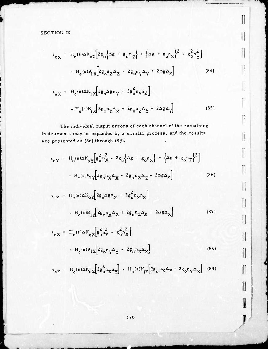
SECTION IX
cX
■sX
- He(8)AKoxK{^ + ßonz} + {Ag + gonz}2 " gonY]
" He(8^x[2gonZAZ " 2gonYAY + 2AgAz]
= He(s)AKlx[2goAgnY + Zg^n^]
" He(s)Klx[2gonYAZ + 2gonZAY + 2AgAY]
(84)
(85)
The individual output errors of each channel of the remaining instruments may be expanded by a similar process, and the results are presented ?s (86) through (89).
LcY = He(s)AKoY[g2n2 - 2go|Ag + g^} + {^g + gonz}2]
1 ( ! ^ i :gonXAX " 2gonZAZ- 2AgAz]
'sY - He(s)AKoY[2goAgnx + 2g2nxnz]
" He(8)KlY[2gonXAZ ' Z*onZ*X + 2AgAx] (87)
«cZ : He(8)AKozLgo4 " go, [22 „2 2 "I KnY " gonxJ
He(s)Klz[2gonYAY - Zg^J (88)
sZ = He(s)AKoz[2gonXnY] " He(8)Klz[:,gonXAY+ Z^Y^ (891
170
fl n
i
i i
i ü
i]
u 1
A /
—

^^^"
r r r
SECTION IX
Substitution of (84) through (89) into (74) and (75) yields the
prime anisoelastic errors at the gravity gradient tensor as shown in
(90) through (95).
H (s)
XX ^—^K .g 3 oY6«
nX + "z -2nZ-2it ^ VZ Uo).
I I
i
i: D i; I 1 I 1 1
H (>) e AKoZgo[nX - 4]
H.(s)/ 2 AgA
nv + Z
g X ' 2 8o g0
He(8)/ Z\{A AX 1 (90)
YY
H_(8)
3 ÄKo -A4- 4] H (■) j 2 u 2n7 -2^-2^1
Z go go •» ■ (€] H (s)
e K4^ - ^] H (•)/
-T-l2" B 2 DC0
A7 Ay AgAZ -nz " g nY + ~T" Bo g0 g.
(91)
171
.^..^.^^BiaBM« Ml

V
SECTION IX
zz He(s) z\ ^r-AKoxgo[n
2 - n2 + 2nv + 2^ + 2^ny ^ (^S) Z Y ^ g0 g0 Z \go/ _
H (s)
H (s)
v§2 2n oYsol
e^'/ 2\
H (s) e K^^)
z - 4 - 4+ ^ ■ *tz ^Y Az ApAZ rnY - Tnz - —r g
7"nz ■ Tnx + ~T 6o 6o g
($
= H (s) XY ev (aKoZ^)"x"Y - (K
1Z4)(^o"x + ^"v)
€ = H (8) XZ e KY^K-Z + tnx)
(K g2)/^ + ^ \ lYKo^ go X go Z
Ae*x\
'o /J
•VZ = He(8) AK ^g oXeo )(vz ^ ^n
Y)
K8') r!nY+ T* AgA,
a "Z 2 80
172
(92)
(93)
(94)
(95)
- - - -- iMM ^^MHl^Hinaii
il
1
i
il
I
!l 1
1 11 1 1 1
11 11 '■
11

▼^
I I 1 r [
D
SECTION IX
fcWXore estimating the standard errors of the gravity gradient
tensor elements, it is convenient to examine the magnitudes of some
of the terms •with the objective of eliminating those that are clearly
negligible. In this process, the following parametric bounds will be
employed:
AK gH < 26. 95 EU o o|
Kt £ 2695 EU
(96)
(97)
A/g, < 10" (98)
Ag/gJ = 3 x lO-3 (99)
First, consider terms of the forms (Ag/g ) and[(Ag/g M&Zg )]
A quick calculation shows that these terms contribute less than
0. 001 EU and may be neglected. Next consider terms where (Ag/g )
is an additive factor in the coefficient of a common term, e.g. , in (90)
the terms -2n„(l - Ag/g ). Clearly, in this case the factor, Ag/g ,
can be dropped without appreciable error. Finally, terms whose
coeffici nts are dependent on the accelerometer instrument errors
(A/g ) are small in comparison to the terms whose coefficients depend
on the error in the prime anisoelastic compensation coefficient (AK )
as shown by (96) and (100).
K.4 A
!o i-^\ < 0.2695 EU (100)
All such terms will contribute on the order of 0. 001 EU or less
and may be neglected. Applying the foregoing approximations to (90)
through (95) yield the simplified gradient tensor errors forms (101) through (106).
173
mm

^
SECTION iX
XX a*4i[{ *K„/O) 4+ 4 ■ 2"z - 2t
YY
zz
K zgo)(4 ■ 4)
He(s)
3 Kzgo)(4 - 4)
+ Kxg2
0)(4-4--z-t)
He(s)
3 Kx4)(4 - 4 + 2nz + zi ;)
K^)h - 4 ■ -i • •¥)
e s H (s) XY e
XZ
YZ
B^OZ^OIVY]
. He(s)[(^KoYg20)(nxnz)]
^ He(8)[(AKoXgo)(nYnz)j
(101)
(102)
(103)
(104)
(105)
(106)-
It should be noted that terms of the form (Ag/g0)n in (94) and
(95) have been neglected in the approximations of (105) and (106) on the
basis that these terms are numerically smaller than other previously
neglected terms.
174
I
1 n
1 1
i
i n
i
i
ft
!
1
■^

SECTION IX
Let us now examine the gravity gradient tensor element errors
for their statistical properties on the basis that the normalized accel-
erations are rero-mean. wide-sense stationary, gaussian random
vanables. For this purpose, assume that all of the prime anisoelastic
error coefficients (AKJ are numerically equal to the upper bound given by (97).
The tensor element bias terms may be written directly in terms
of the acceleration covariances evaluated at zero time shift as in (107) through (HZ).
M AK g2
o6o XX 2C (o)
X Cv(o) + C (o) - 2^i Y Z go ] (107)
M YY
AK g2
o6o 2C (o)
Y Cx(o) " Cz(o) " zi (108)
D [ I I \
1 1 1
M AK g
o6
ZZ L go cx(o) - C (o)
M
M XZ
M YZ
C (o) XY
C (o) XZ
iAKo8;;cyz(o)
(109)
(110)
(111)
(112)
The trace element bias functions are characterized by a trend,
i. e.. the (Ag/go) term whose magnitude is proportional to altitade
change from the initialization point. When this term has the magnitude
given by (99). a bias of 0. 054 EU is contributed to the horizontal trace
1 175
mm

MP
SECTION IX
elements and 0. 108 EU to the vertical trace element. The remaining
parts of the bias terms depend on the acceleration covariances. It is -4 2 estimated that all acceleration variances will be bounded by 7 x 10 g
in the operational environment. This leads to a trace element bias
bound of approximately 0. 013 EU and a cross-element bias bound of
approximately 0. 019 EU due to the acceleration variances. A summary
of the total biases on each tensor element is given by (113) through
(H8).
M !<. 0.067 EU xx'
M ! < 0. O^ EU i YYI
K; < 0. 121 EU
M 1 < 0.019 EU I XYl
M < 0.019 EU I xzl
M < 0.019 EU I YZI
(113)
(114)
(115)
(116)
(117)
(118)
Observe that the largest bias errors occur in the trace elements
and that they are primarily the result of the scalar gravity trend.
To compute the tensor element variances, it is convenient to
assume the normalized accelerations to be statistically independent.
This 'assumption has a small effect on the resultant errors because the
most significant errors aie due to the linear term (n7) in the trace
element error equations. Now, we consider the power spectrum of
=. assuming the (AK g 1 coefficients are numerically equal.
176
ii
i
1 1 8 1
1
fl r
J *0M iMM

SECTION IX
1 S (f) = -S-IH (s)|2fÄK g2l r4S,*S + S *S 4 S *S + 4sJ(119) XX 91 ev 'I L o8oJ LXX YY ZZ zJV7'
r. i
I I i:
When all the acceleration spectra are assumed to be of the same
amplitude and shape, equation (119) reduces to (120).
S (f) XX
^|H (s)|2fAK g2] ["45 (f) + 6S *S 1 (120) 91 e I L o6oJ L n n nj y
The remaining spectra may be written on the same basis and
are presented as (121), (122), and (123),
S (f) = -JIH (S)I2(AK g l^S (f) + 6S *S 1 (121)
YY 91 e I L o6oJ L n n nj
S (f) = Uu (s)|2fAK g l2fl6S (f) + 6S *S I (122) ZZ 91 e^ I L o5oJ L nw n nj
S = S XY XZ
S^^ = lH (S)|2[AK g2l [s (f)*S (f)l (123) YZ I e |l L o0oj L n n J
(.
The error variances are obtained by integration of the error
spectra. Two spectral forms must be considered, i.e., the accelera-
tion spectrum itself and its convolution, as in (124) and (125).
/to
IH (j2Trf )l 2S mdf 1 e ^ I n 00
(124)
nn
/CO
IH (j2iTf)|2S (f)*S (f)df 1 e J I n nv
00
(125)
177
"MHM
MMfl^a jam*

SECTION IX
It is assumed that S (f) is constant below 1 Hz with a n -4 2 "two-sided" amplitude of approximately 2. 8 x 10 g /Hz. On this
basis, the integral of (124) is stated as (126).
I s (2. 8 x 10 )Af n e 1.4 x 10_5g2 (126)
The integral of (125) may be approximated by assuming the
acceleration spectrum, S (f), to be constant between ±f and zero r n o outside of this band. This appn ximation is stated as (127).
I s 2f (2.8 x 10"4g2/Hz) Af nn o 6 « (127)
The frequency, f , may be eliminated from (127) by its relation 0 2 to the acceleration variance, cr , as in (128). n
n 2f (2.8 x 10"4g2/Hz) (128)
11 i
1 I 1 n
:!
1 Ö
In computing the bias terms an acceleration variance of -4 2
7x10 g was employed. Substitution of this value and (128) into
(127) yields the desired integral as (129).
Inn a (7 x 10'4g2)(2.8 x 10"4g2/Hz)(0. 05) = 10"8g4 (129)
Comparison of the resultant integral values of (126) and (129)
provides an indication of the dominance of the linear terms over the
non-linear terms in the prime anisoelastic error variances.
Substitution of the integral values of (126^ and (129) for the
appropriate integrals of the error power spectra of (120) through (123)
yields the standard "prime anisoelastic" tensor errors due to the
VIALS as shown i ^30) through (133).
178
!
9
II D }
mm ^—M

1 I
I I 1 1 I r r.
i
i
r i
i \
i
SECTION IX
o- a (26^5W(4)(1#4)(10-5) + (6)(10_8) St 0.068 EU (130) XX \ 3 /
YY s /2k95\(7>5 x JO"
3) -0.068 EU (131)
o- a (26^95) \/(l6)(L4)(1o-5) + (6)(10"8) H 0. 135 EU (132) zz \ 3 /
a- =0" = a XY XZ YZ
Si (26. 95) VlO"8 M 0.003 EU (133)
A summary of the standard anisoelastic errors at the gravity-
gradient tensor elements is presented as Tables IX-6 and IX-7 for RGG
spin bearing excitation and for VIALS excitation.
TABLE IX-6
Anisoelastic Errors 'Spin Bearing)
"xx •"YY ^ZZ '"XY "xz "YZ
Cross-Aniso
Prime-Aniso
0.011
0.013
0.011
0.013
0.009
0.018
0. 014
<*>
0.010
0.019
0.010
0.019
TOTAL 0.017 0.017 0.020 0.014 0.021 0.021
TABLE IX-7
Anisoelastic Errors (VIALS)
"xx YY ffzz "XY
Txz ^YZ
Cross-Aniso
Prime-iiJiiso
0.013
0.068
0.013
0.068
0.010
0. 135
0.016
0.003
0.011
0.003
0.011
0.003
TOTAL 0.069 0.069 0. 135 0.016 0.011 0.011
i_ T835
179
•m
mtrnm—m

am
■
SECTION IX
G. PLATFORM ORIENTATION ERROR PROPAGATION
Misalignment of the RGG eystem measurement frame from its
nominal refe.-ence position produces errors in the measured scalar
elements of the gravity gradient tensor. These errors may be calcu-
lated as the incremental changes of the scalar elements of the measured
gravity gradient tensor from their values at the point of system initiali-
zation due to coordinate misalignment. The measured gravity gradient tensor elements may be expressed
as a matrix, [r ], in terms of a similarity transformation on the actual
gravity gradient matrix, [rj, and the direction cosine matrix, [CJ,
which relates the measurement frame to the reference frame as
in (1).
\]
w - -
)
I
[rj = [c][ra][tf (1)
When the misalignment angles are sufficiently small, the direc-
tion cosine matrix may be approximated to first order by (2) as the sum
of the identity matrix, [l], and a skew symmetric matrix, [4>], defined
by (3).
[C] » [I] + M (2)
*, <t>.
[♦] ^ -♦.
♦,
* X (3)
•«t».
\
1
1
•• Also, observe that the transpose of (2) and (3) may be expressed as (4)
and (5).
180
;
]
:
/
MMM ^^

I I 1 1 1 I
f
i r
i i i
SECTION IX
[C]1 ä [I] + M (4)
|T
Substitution of (2), (4) and (5) into (I) yields the first-order measure,
ment increment due to angular misalignment expressed as (6).
(5)
[rj - W - WLrJ - [rJM (6)
The change in the measurement increment from the point of system
initialization is defined as the gradient tensor error due to misalign-
ment as in (7).
W ^ IFJ - [rjl - ^mo] - [rao]l (7)
Substitution of (6) into (7) yields the expanded error form of (8).
[re] = IW[ra] - [ra]W| lC*0][rao] - [rJC^l (8)
Since the platform misalignment angles are specified in terms of initial
misalignments and changes thereafter, it is convenient to express (8) in
terms of the initial and incremental parameters defined by (9) and (10).
(9)
(10)
Substitution of (9) and (10) into (8) yields the convenient error form of
(11).
[re] = [<i>o][Ara] - [Arjtg + [A<t.][ra] - [rj^] (11)
181
•mmmm

SECTION IX
Expansion of (11) yields the gravity gradient misalignment error set expressed as (12) through (17).
reXX = 2<*ZoArXY ' MYoArxZ + 2A^r~" - 2A<I,.X.- (12) Z XY Y iCZ
eYY Xo Yz Zo XY X YZ VZ XY (13)
^eZZ = 2*YoArxz " 2*XoArYZ + ^VxZ " '^VYZ
(14)
reXY = ^Zo^^Y " Ar-J + 4,--Ar— • «I».. *r XX" Xo XZ ^Yo YZ
+ ^VY ■ rxxl + 4*xrxz " A*yrYz (,5)
reXZ ' ♦yof^XX " ^ " *Xo*rXv * *Z^Z
+ 'i*v[iVv - r ] . a* r + a* r Y XX Z2J X XY Z YZ (16)
^YZ = *x>rzz " ArYY] + *YoarXY " *ZoirXZ
+ A*X[rzz " rYY] + ^VxY " a*zrxz ,17)
For the purpose of statistical analysis of thio error set, it is
convenient to observe that the tensor element errors are linearly
related to the initial and incremented misalignment errors and that the
entire error set may be expressed in the state variable form of (18),
wherein the [A] matrix contains the gravity gradient tensor elements,
rv, and their incremental changes, AF.., from the initialization point. J
[A]* (18)
182
1
'I
!j
1 1
1
1 1 1 e v
i
i
j

]
I
I I i i
i i i
SECTION IX
The gravity gradient error covariance matrix, [r], may be expressed
in terms of the misalignment angle covariance matrix, [*] as (19).
LIT] = MOM (19)
The trace elements of (19) correspond to the gravity gradient
tensor element variances of the errors of (1?) through (17). Rigorous
evaluation of the trace elements of (19? requires complete knowledge of
the misalignment error covariance matrix, [*], as a function of time.
An approximate estimate of the trace elements of (19) may be obtained
using the specified variances of the initial and incremental platform
misalignment angles as stated in (20).
frl.. a 5a2.*.. LU Jii " L*/ lj JJ (20)
Expansion of (20) in terms of the coefficients in (12) through (17) yields
the set (21) through (26).
'XX = ^x/*" + ^V'^S + ^XZ^SS + V^]'21'
^Y = 4[(Aryz)2*11 + (Arxv)2»33 + <rv/*44 + ^x/*"] (221
4 = 4<4rYZ>2*.. t ^XZ'2*" + (rYZ|2*44 + "x/*"](23)
XY (Ar J2*!, + (^ )2*22 + (ArYY - A^ *i3
.2. . -_ .2 - - ^ + (rxz)^44 + (rj *65 + (rYY - rxx) *66 (24)
183
^^ MMMMfli tmamm mmmmm

V ■ ' ^ !
SECTION IX
XZ XY ^rvY>Z*ll+ '^XX-^ZZ1 *22 + '^YZ' *33
, 2 2 + (r r* + (r • r ) «re + (r ) *,/
XY (25)
cr2 = (AF - AF )2*n + (^IVJ2*22 + (ArxZ)2*33 YZ ZZ YY 11 XY ^^ Ä^
+ {rZZ ■ rYY)2*44 + ^x/^S + (rxZ)2*66 (26)
Evaluation of (21) through (26) is facilitated by substitution of
the specified misalignment angle variances as defined by (27), (28), and
(29).
■K]M*vol4['-5'l0-f * *n-*"
E[^] * E[^^ 4 [5 x .0-5]2 S . 44 55
441 = EK] ^ [5 ^io-4]2 = * 33 " *66
(27)
(28)
(29)
Now let us define the parameter, o-^, by (30) and the covariance par
etersby (31), (32), and (33).
% ^ 5 x 10"5 r»d
<S = $ = 25(j'. ^11 22 <t>
*33 = *66 = 10%
am-
(30)
(31)
(32)
184
I
"I ]
1 '1 "1
ö
I
0
B fi (!
J

I I 1
1
r r i
SECTION IX
*44 = *55 = % (33)
The estimated gradient tensor standard errors may be expressed
as (34) through (39) by substitution of (31), (32), and (33) into (21)
through (26) and taking their square roots.
XX
-.1/2 a 2^[25(Arxz)2 + ioo(ArxY)2 + (rxz)2 + ioo(rxY) J (34)
YY «2^[ ■> 2l1/2
25(Ar.j2 + ioo(Ar.j2 + (r_r + ioo(rvv) J (35) YZ XY YZ XY
\za 2^25<Arv/ * "'^xz1' + ,rv/' + 'Sc/] k 1/2
YZ (36)
D r.
XY ♦
^XZ « ^
25(Arxz)2 + 25(ArYz)2 + Joo(ArYY - Arxx)2
+ (rXZ)2 + ^YZ^ + 10Ö(rY.Y - W
25(Ar )2 + 25(Ar v - Ar / + ioo(Ar )
1/2
(37)
XY XX ZZ YZ
+ (r )2 + (r - r „)2 + ioo(r J2 v XY XX ZZ YZ
1/2
(38)
1 1 I 1
YZ <J>
25(Ar - Ar )2 + 25(Ar )2 + ioo(Ar ) ZZ YY XY xz
+ (r - r )2 + (r )2 + ioo(r J2 T V'-rfT 1W' l*W V7 ZZ YY XY XZ
1/2
(39)
185
■i i i m-
^^ mmm

SECTION IX
Numerical evaluation of (34) through (39) requires definition of
the error coefficients, P.. and AT... For this purpose, we make the ij ij r r » following arbitrary definitions:
;
•
1. Operating Point Values:
r XY XZ
r - r YY XX
r YZ
150EU
= 300EU
r - r ZZ YY XX ZZ
2. Incremental Change Values:
4500EU
(40)
(41)
(42)
AT XY
Ar - Ar I YY XX
AT XZ
ArZZ " ArYY
AF YZ
300 EU (43)
Arxx " Arzz H 600EU
(44)
Substitution of the numerical values of (30) and (40) through (44)
into (3^) through (39) yields the estimated gravity gradient tensor ele-
ment errors stated as (45) through (48).
o- s o- 3 0.368EU XX YY
<r M 0. 212EU ZZ
a s 0. 3 52EU XY
o- a o-,,,, a 0. 327EU XZ YZ
(45)
(46)
(47)
(48)
- ■
1 1
1 8 [|j
i
f)
It is realized that the equality of (42) requires that (41) be zero; however, the equality of (42) is assumed for analytical simplicity.
186
(i
J *mk

rwvw
I I i
0
I I 1
SECTION X
SENSOR ROTOR DESIGN
The objectives in designing the rotor were to make it as small,
rigid, symmetrica', and homogeneuus as possible. At the same time,
provision for initial assembly test and balance was necessary. The
design evolved into a main circular central plate to which all other
parts could be fastened symmetrically. Except for the pivots and fas-
teners, the rotor is entirely of 6061 aluminum, which provides good
heat conductivity and symmetrical thermal expansion. The good heat
conductivity reduces thermal gradients to a minimum.
All fasteners will be made of beryllium copper and will be
designed so that the fastener is in tension. Since Be-Cu has a lower
thermal coefficient of expansion than aluminum, when the sensor is
assembled at room temperature and then raised to operating tempera-
ture, the fastener will be tightened. The pivots are made of Be-Cu
because the temperature coefficient of the shear modulus of elasticity
is much lower (-330 ppm/ C) than for most other metals. This aids in
keeping the thermal sensitivity of the sensor urdamped natural fre-
quency to a minimum.
A. DESCRIPTION
This paragraph refers to Fig. V-l and the number flags ofthat
figure. However it provides more detail than the Section V summary.
The circular central plate (3) and the eight brace posts (5) are machined
from a solid billet of aluminum. The pivot structure (4) is made from
a single rod of beryllium copper and is attached at the center of the cen-
tral circular plate. At this point the assembly appears as a circular
central plate with four symmetrically arranged brace posts protruding
from each side. The pivot structure appears as two more posts cen-
tered in the plate. The pivots extend slightly beyond the brace posts.
187
^^^

SECTION X
The arms and arm masaes (7) can now be assembled onto the
pivots by ii Lerleaving the arms in the proper order. Prior to this
assembly, each arm has had the remote mass balance assembly (10)
and the appropriate transducer stand-off posts (23) installed. The end
plates (6) can now be attached to the brace postn (5) and to the outboard
end of the pivots. The assembly now appears as a central plate with a
cage-like structure protruding from each side. The outer end of the
cage is the end plate (6). The end plate and the central plate support
and hold the pivots and the pivots in turn support the arms and their end
masses. Eight transducer mounting posts (23), arranged in a circle,
extend through each end plate.
A holding fixture is now provided. This holding fixture is a
cylindrical tube that fits into the circumferential ledge at the outer
perimeter of the central plate. The holding fixture is a dummy end bell
with a flat open end and access holes bored through the cylinder walls.
The central assembly can now be placed on the holding fixture and one
set of transducer mounting plates (22) and transducers (8) installed.
The other end is completed in a similar fashion. The rotor electronics
assembly (9) is installed at this point and internal wiring completed. A
battery pack will be installed on the cylindrical holding fixture and
temporary connections made to the electronics pack so that the FM
signal can be brought out. The central rotor and arm structure can
now be tested for arm unbalance, arm anisoelasticity, and transducer
and test signal operation. Adjustments can be made as required.
After all internal adjustments have been made, the rotor end
bells (1) are installed. These end bells have been provided previously
with the female part of the spin bearing (2), the encoder disk (12), the
two test signal photocells (15), the spin motor/tachometer (11) drag
cup, and the FM output antenna (16). This completes the rotor
assembly.
I li 1
i
-
I
!
!
i 1
188
J ■A ^MÜ

«p^
I I 1
B I
SECTION X
B. STIFFNESS, MASS, AND INERTIA CALCULATIONS
Detailed calculations for stiffness, mass, and inertia have not
been made for the RGG prototype design. Preliminary values, believed
to be sufficiently accurate for all but final modelling, are as
follows:
Axial stiffness
Mass, including arm»
Inertia, including arms I = I jxx yy zz
175 x 106 N/m (1 x 10⁶ lb/in. )
5. 867 kg
1.44 x lO"2 kg m2
2.039 x lO"2 kg m2
i:
i
i
I i i
189
-«MOT
■^ ■lll'M .«lIT-gl

I I I !
1
i
■
r
l i
i i i
SECTION XI
SENSOR STATOR DESIGN
A. GENERAL
The purpose o( the stator is to provide a stable, indexed mount
for the sensor; to protect and restrain the rotor; and to locate the spin
motor/tachometer, encoder light source, test signal light source and
the FM receiver antenna.
This paragraph refers to Figure V-l and the number flags of
that drawing. The material selected for the jtator is 6061 aluminum,
the same as that of the rotor. A sturdy flange (18) provides a rigid
flat mounting and index surface. The motor/tachometers and the male
parts of the spin bearings are mounted in the end caps (19). One end
cap is insulated from the remainder of the stator by a thin mica washer
(20). This allows the rotor electronics power to be coupled into the
rotor through the capacity between the spin bearing halves and between
the motor stator to drag cup as described in Section XV. The test sig-
nal light source (14) is positioned to illuminate the two rotor mounted
test signal photocells (15). The rotor position light source and photo-
cell (13) is positioned so tha- the encoder disk on the rotor (12) can
interrupt the light beam and produce the precise 1 /8-revolution signals
required by the system. The FM receiver antenna (16) is mounted on
the end opposite to that just discussed.
One of the most critical sensor dimensions is the axial clearance
of the spin bearings. This is adjusted during assembly by initially
making the clearance '.oo large. Then, with the sensor stabilized at
operating temperature, the clearance is measured by means of the
capacitor clearance gauges built into the spin bearing. The end cap is
then removed and the spacer or shim ring (21) is lapped to the required
dimension. A selection of spacer rings will be made initially and one
near the proper dimension will be selected for the first assembly. This
completes the stator assembly.
Preceding page blank 191
'"
M-^aMa ^mt*ma^ma

I
SECTION XI
B. STIFFNESS, MASS AND INERTIA CALCULATIONS
Detailed calculations for stiffness, mass, and inertia have not
been made for the RGG prototype design. Preliminary values, believed
to be sufficiently accurate for all but final modelling accuracy are:
.8 Axial stiffness
Mass
Inertia
•xx zz
= I yy
1. 58 x 10 N/m (9 x 10⁵ lb/in. )
3.766 kg
2.89 x 10² kg m2 2. 53 x 102 kg m2
192
L
■
7
B :
i
/
a^^^afl^ia

SECTION XII
SPIN BEARINGS
I
i:
The previous Hughes RGG "hard bearing" sensor experimental
development program had utilized a commercially available hydro-
static air . jin bearing manufactured by Professional Instruments Co.,
Minneapolis, Minnesota, and designed for machine-tool spindle appli-
cations. Although this program had provided promising results, no
tests were conducted that allowed separation of the spin bearing con-
tribution tc the lowest sensor noise level achieved (6 EU). Realizing
the importance the spin bearing would play in determining the overall
sensor accuracy, we sought the best professional assistance available
in selecting and designing the optimum bearin? type for the prototype
sensor.
Characteristics, error mechanisms, .ind requirements that
affected the spin bearing design were studied and formed the basis of
a procurement specification. These studies and the procurement speci-
fication are contained in the Semiannual Technical Report No. 1 (see
Section V-C). A bearing vendor survey was made, proposals requested,
and a vendor was selected. The vendor. Mechanical Technology
Incorporated (MTI), Latham, New York, was placed uncer contract
on 24 July 1Q72. This contract called for a bearing trade-off study
and selection recommendation followed by generation of a detailed
design and a design specification for the bearing.
MTI has completed this effort and has prepared a final report
entitled, "Spin Bearing Selection and Design for Hughes Research
Laboratory Rotating Gravity Gradiometer," Ref. No. MTI 72TR59,
October 1972. In addition to this report, MTI has generated a design
specification, which is included as Appendix D herein. A summary
of the candidate bearings considered in the trade-off study and the
rationale leading to the selection of the prototype bearing type is
presented in the following oubsections.
193
•mmmm..

SECTION XII
A. BEARING CANDIDATES
Initially, 12 bearing types were considered: 3 bearing
geometries — cylindrical, conical, and hemispherical; 4 lubrication
methods —hydrostatic gas, hydrodynamic gas, hydrodynamic oil/
grease, and squeeze-film. This initial group of 12 was quickly nar-
rowed to three candidates. The squeeze-film type was found unaccept-
able because: (1) the power to operate it was excessi e, and (2) the
stiffness would be too low. The hemispherical geometry was selected
over the conical and cylindrical types on the basis of the following:
(J) easier alignment of the two bearings, and (2) ease of producibility.
B. BEARING SELECTION
Having narrowed the choices to three hemispherical types
(hydrostatic gas, hydrodynamic gas, and hydrodynamic oil/grease),
MTI proceeded to perform more detailed studies of these three types.
These detailed studies indicated the design and performance character-
istics of each bearing type. The performance and size of both air
bearing types were virtually equal in all respects except the breakaway
torque requirements. The breakaway torque for the hydrostatic bear-
ing was virtually zero. The breakaway torque for the hydrodynajcnic
gas bearing was 130 in.-ozs, approximately 20 times larger than the
capability of a practical sized spin motor of the drag-cup type consid-
ered appropriate. Both bearings had diameters of approximately
3 in. The large breakaway torque of the hydrodynamic gas bearing
(due to its large friction radius arm) resulted in its being dropped
from further consideration.
The performance characteristics of the remaining two bearing
types, hydrostatic gas versus hydrodynamic oil/grease, were essen-
tially equal, again except for their breakaway torque requirements.
The oil/grease bearing required 5 oz-in., which was slightly less
194
0 0
0 0
i
i
i
S s }
^äm
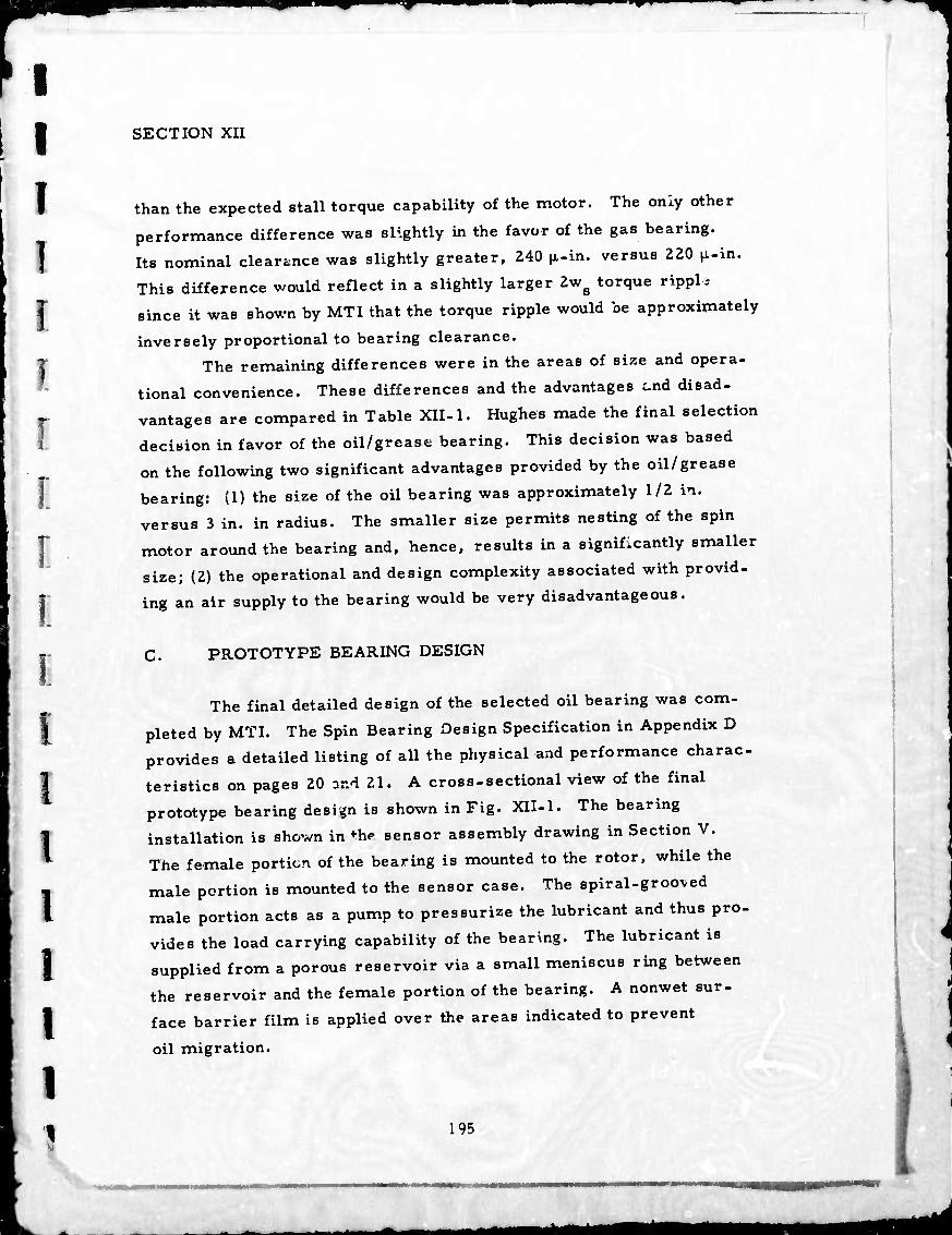
'i^ • *m*
I I 1 1 f T
I r.
i {
\
i
i
i
SECTION XII
than the expected stall torque capability of the motor. The only other
performance difference was slightly in the favor of the gas bearing.
Its nominal clearance was slightly greater. 240 n-in. versus 220 ji-in.
This difference would reflect in a slightly larger 2w8 torque ripple
since it was shown by MT I that the torque ripple would be approximately
inversely proportional to bearing clearance. The remaining differences were in the areas of size and opera-
tional convenience. These differences and the advantages end disad-
vantages are compared in Table XII-1. Hughes made the final selection
decision in favor of the oil/grease bearing. This decision was based
on the following two significant advantages provided by the oil/grease
bearing: (1) the size of the oil bearing was approximately 1/2 in.
versus 3 in. in radius. The smaller size permits nesting of the spin
motor around the bearing and, hence, results in a significantly smaller
size; (2) the operational and design complexity associated with provid-
ing an air supply to the bearing would be very disadvantageous.
C. PROTOTYPE BEARING DESIGN
The final detailed design of the selected oil bearing was com-
pleted by MTI. The Spin Bearing Design Specification in Appendix D
provides a detailed listing of all the physical and performance charac
teristics on pages 20 and 21. A cross-sectional view of the final
prototype bearing design is shown in Fig. XII-1. The bearing
installation is shown in *hp sensor assembly drawing in Section V.
The female portion of the bearing is mounted to the rotor, while the
male portion is mounted to the sensor case. The spiral-grooved
male portion acts as a pump to pressurize the lubricant and thus pro-
vides the load carrying capability of the bearing. The lubricant is
supplied from a porous reservoir via a small meniscus ring between
the reservoir and the female portion of the bearing. A nonwet sur-
face barrier film is applied over the areas indicated to prevent
oil migration.
195
MflH ^m* Ü mm

OB*
SECTION XII
TABLE XII-1
Final Spin Bearing Selection Considerations
Hydrostatic Air Bearing Hydrodynamic Oil Bearing
Advantages Disadvantages Advantages Disadvantages
1. Low break- 1. Very large 1. Small — easy 1. Higher break- away torque. size: to package
motor and away torque.
2. Approxi- a. Difficult smaller 2. Drag and mately 20% to design senior size. ripple torque lower ripple and make temperature torque. motor. 2. Convenient — sensitive,
no air supply /. must con- 3. Bearing b. Significant problems.. trol bearing
exhaust air increase temperature would help in sensor 3. Cost is more cool sensor. size. slightly less. closely.
(Not incon- 2. Has drag and sistent with
ripple torque temperature sensitivity to control supply air requirements pressure and on sensor. temperature. however.) .*. requires close control 3. Must conduct of both pres- fll develop- sure and ment tests at temperature operating of supply temperature. air.
4. There is a 3. Air feed considered
across plat- risk in oil form gimbals recirculation very difficult and retention. and opera- May require tionally periodic inconvenient. replenishment.
4. Loss of air supply could damage bearing.
T873
196
h
i
i
1
B
1 i
1
i
i]
■i
11 (1 '1
2 tfta^rfa *m **■*

r i i
HBP" JL
1 I
I 1
CEMENTED JOINTS
NONWET SURFACE BARRIER FILM
CEMENTED JOINTS
207ft-54
MALE BEARING COMPONENT
OIL RESERVOIR
FEMALE BEARING COMPONENT
Fig. XII-1. Spin Bearing Final Design Cross-Sectional View.
197
NNP"
- ■ ^M *^^^B*
WW^'
SECTION XII
Some of the bearing performance requirements were restated
in this final specification. These were necessary to reduce the
mechanical tolerance requirements imposed by the original Hughes
procurement specification. The nature of these changes was to allow
specific RGG errors, induced by the spin bearing, to be increased
provided the resultant RGG error would be deterministic. The allowed
randomness of these errors, induced by the spin bearing, was not
modified. Thus, the deterministic portion of these errors will be
"biased-out" during the sensor calibration operation.
The spin bearing performance requirements imposed in the
RGG sensor application are difficult, but are within the state of the art
of bearing technology. Manufacture of the bearing will require close
control and surveillance by competent technical personnel.
i 1 !
0 1 I
1 \
1 1
198
'
*mM mmm

I SECTION XIII
i I I
SENSOR ARM DESIGN
[
1 I I I I I
A. GENERAL
The following major factors were considered in selecting an
optimum design configuration for the RGG sensor arm pair: thermal
noise, size, weight, structural resonant frequencies, isoelasticity,
mass/structural symmetry, and compatibility for mounting mass bal-
ance adjustment devices and the gradient signal transducers.
Nominal sensor design parameters, selected early in the sensor
design process, allocated approximately one-third EU to thermal noise.
Thus, the arm size-weight characteristics were established.
Since arm anisoelasticity was one of the potentially large error
sources for the moving base environment, selection of the basic arm
structural configuration was heavily influenced by this characteristic.
Similarly, because of potential dynamic coupling between arm struc-
tural vibration modes and both external and internally generated vibra-
tions, a light-weight, high stiffness arm structure, having relatively
high natural frequencies, was desired. A requirement for symmetry of each individual arm structure
placed one constraint on design of the arm pair. A nonsymmetrical arm
structure can cause a see-saw motion of the arm (oscillatory angular
motion about an axis normal to the spin-axis), induced by external
translational vibration, which results in a 2 w differential arm gradient * 8
error torque. Another error source, axial arm mass unbalance, imposes
the requirement that the center of mass of each arm be coincident, both
*See HRL Technical Proposal 71M-1593/C3755, September 1971, pp 355-364.
**See Section IX-A.
m
199
MM^UMi ^^^ riHDMÜ M

1
SECTION XIII
radially and axially. This error is proportional to the product of axial
center of mass separation distance and radial center of mass separation
distance. Hence, it was only necessary to make this product sufficiently
small. Finally, it was necessary that the arm design provide for mount-
ing of the mass balance adjustment devices and for connection and
mounting of the output transducer. The desired location of the mass
balance adjustment devices waa near the center to minimize centrifugal
forces imposed on them by the spin. The transducer mounting scheme
was selected to minimize all mechanical loading on the transducer
except that caused by axial differential arm torque.
The material selected for the arm structure is aluminum, while
that for the end masses is Mallory 1000. The justification for these
choices is contained in Section II.
3. FORM FACTOR TRADEOFFS
Ideally, a long slender arm structure with relatively small sized
end masses would have the highest inertia efficiency, T] , and the least
mass. However, the requirement for an isoelastic structure with high
resonant frequencies suggests a short stubby form factor, but would
have a higher total mass. A solid bar of rectangular cross section can be
shown to be anisoelastic no matter what its length to cross-sectional
area ratio may be. Such a structure deflects in shear about three times
more than in compression. See Fig. XUI-l. This is because the shear
modulus is usually about one-third the Youngs moduluo. Considering
any flexural bending deflection just makes this ratio of lateral to longi-
tudinal deflection even more unequal. Hence, a solid arm structure to
support the high density end masses cannot be isoelastic. A structure
with cutouts of some kind, to weaken it more longitudinally than later-
ally, is required. Also, to keep the axial bending (end mass deflection along spin-
axis direction) and see-saw stiffness high, it is desired to keep the depth
200
i
0 I
1 1 ]
2 i
B 0 "i
1 1
,1
—

^■F-i,
SECTION XIII
I
I
t
of the arm structure large. Figures XIII-2 and XIII-3 illustrate two
possible arm designs which can meet these isoelastic and high stiffness requirements.
To keep the overall sensor length small and simultaneously pro-
vide for high see-saw and axial bending stiffnes.-j, it is desired to inter-
leave the two arms. Two possible configurations are shown in Fig.
XIII-4(a) and (b) for the individual arm configuration shown in Fig. XIII-2.
Note that for either interleaved configuration shown, the arm width must
be lesjj than tha longitudinal distance between the end masses.
The interleaved configuration shown in Fig. XIII-4(a) has the
advantage that each arm can be made identical. The configuration of
Fig. XIII-4(b) requires two separate arm designs to achieve equal iso-
elastic parameters for each. In configuration XIII-4(a), the arm cen-
ters of mass are separated axially which gives rise to an error sensi-
tivity to angular accelerations normal to the spin-axis. However, error
analyses have shown that this sensitivity is sufficiently small. In the
configuration of Fig. XIII-4(a), the inner arm will have a considerably
lower "see-saw" stiffness than the outer arm. This low stiffness could
give rise to "see-saw" motion of the arm, induced by a small arm axial
center-of-mass offset acted upon by translational acceleration normal
to spin-axis, which results in a 2 w differential gradient error torque.*
The arm configuration of Fig. XIII-4(b) has been selected for the proto-
type arm design because of its higher achievable see-saw stiffness and
because each arm is of identical design.
Tradeoffs between the arm configurations of Figs. XIII-2 and
XIII-3 pertain to anisoelastic design considerations and are discussed in Section XIII-D.
C. ARM MASS AND INERTIA EFFICIENCY
The physical size and weight of the total RGG sensor package is,
to a very large extent, dominated by the dimensions of the sensor arms.
::See HRL Technical Proposal 71M-1 593/C3755, September 1971, pp 355-364.
201
M^M« ^■rti

ton-IO
Flg. XIIU1. Solid Bar Structure of Rec- tangular Cross Section.
«0T8-SI
Fig. XIII-2 Arm Configuration A.
202
1 1 ]
1 il 1 1 1 I 1 \
1 1 8
n !
1
J i ^^^m^mmM

«075-5t
Fig. XIII-3. Arm Configuration B
203

WNMUWIUW-IIP
20T5-33
(0)
(b)
Fig. XIII-4. Arm Configuration - Interleaved.
204
i I
1 1 1 1
1
0
11 II 1
]!
•
^^^

^r
'
I
SECTION XIII
The allocated 1/3 EU ihermal noise limit imposes the requirement that
H C be at least 26,400 gm-cm". This requirement could be met by zz
many combinations of arm end mass vs arm length, and hence a trade-
off between these two parameters is implied. Because of the many form
factor considerations, a rather short stubby arm configuration is pre-
ferred. Also, since the total sensor weight tends to be proportional to
the third power of the arm's largest (radial length or axial height)
dimension, arm size rather than mass has the greater influence on
over-all sensor size and weight. Furthermore, an optimization study
which determined the best combination of arm length, width, and height
to maximize the n C parameter indicates that a short stubby form is ' zz r
optimum. This would appear surprising at first glance until it is real-
ized that the inertia efficiency factor, r\ = (B yy
A )C , plays a xx zz' r 7
dominant role in the n C parameter. zz The results of the optimization study are depicted graphically in
Fig. XIII-5. Note the strong dependency of r| C on arm width to
length ratio, a/2R. The optimum value of width to length ratio is depend-
ent on the ratio of the mass length to overall arm length, b/R, however
for 1/3 < b/R < 2/3, the optimum changes only very slightly. For
the prototype armdesLgn, b/R was chosen as 1/3, and a/2R as 1/2.
It is interesting to note that height, £, and the plate thickness,
t, play a very insignificant role in determining this optimization. It
can be shown that TJ C of the heavy weight masses alone is completely z z independent of their height, i. The second order effect of varying the
tp. /^p? ratio is brought about by the influence of the additional mass and
inertia of the low density arm structural material. The ratio of the
weight of the arm structure to the heavy weight end mass material for
the prototype arm design is approximately 1/6 th .
The trends determined from the optimization study are applicable
to either of the arm configurations of Fig. XIII-2 or XIII-3. The dimen-
sions of the prototype arm were chosen by: (1) selecting a/2R and b/R
ratios consistent with the optimization curves of Fig. XIII-5 at
'The calculations leading to the specification of this number are shown in the Semiannual Technical Report No. 1, p. 72.
205

tOTt-14
T T ARM INERTIA PARAMETER VS. WIDTH TO RADIUS RATIO
0.4
0.3
N o
0.2
0.1
^ Byy~AK«
0.02
0.2 0.4 0.6
a 2R
Fig. XIII-5 Arm Inertia Parameter Versus Width to Radius Ratio.
206
!
I
1
1
.i
■
I
i
i
f
- «MOMfe

V~m
i.
'
I
SECTION xm
a/2R = 0.5andb/R = 1/3, (2) selecting for the materials, aluminum
for the arm structure and Mallory 1000 for the end masses, (3) selecting
an arm structure thickness of 0.25 in., and (4) trading off arm radius,
R, with height, i, to result in an arm configuration which provided the
required T^C value and which had the appropriate ratio of R to £ to
minimize the radius of a circumscribed sphere. This approach was
used to minimize the volume, and hence weight, of the surrounding rotor
and case. After selecting the primary arm dimensions, it was noted that if
a cylindrical or spherical rotor were used to house the arms, additional
inertia efficiency could be obtained by merely adding a cylindrical sec-
tor portion on each arm mass as shown by the dotted linea of Fig.
XIII-6. Addition of this sector reduced the radius of the circumscribed
sphere by 8% and ■,.creased the inertia efficiency, r\, from 0.83 to 0.86.
Finalizeddimensions, weight, and moments of inertia of the base-
line arm design are summarized in Section XIII-E.
D. ISOELASTIC ARM DESIGN
Many arm structural configurations have been considered during
this study, some quite simple and some, although possibly superior in
concept, very complex and extremely difficult to fabricate and assemble.
The goal established for selecting a suitable design was that it be rela-
tively easy to manufacture and assemble, result in minimum structural
resonant frequencies of approximately 10 to 20 times the gradient sen-
sing frequency of 35 Hz, and be simple and straightforward to trim, in
the laboratory, into final isoelastic balance. After considering the many form factor trade-offs mentioned
above, the two-arm configurations shown in Figs. XIII-2 and XIIi-S
remained as suitable choices. Initially, the arm of Fig. XIII-3 appeared
superior and a detailed structural deflection analysis was undertaken of
this configuration. The re&ults of this analysis showed that for a rea-
sonable overall arm height of 2 inches, isoelasticity could not be
207
flM-1 *■*

tors-se
i 1
/ \ / / 1
\ \ |
1 1 I \ \
t 1 /
/ \ f
i
1— i 1 •—i
1—■ ---i
i
1
B
r— L .
Fig. XIII
i
-6. Arm Mass with Added Cylin- drical Sector Po» 'tion.
208
J

I SECTION XIII
achieved. It had been thought that by varying the inclination angle of the
arm struts, the longitudinal to bending stiffness ratio could be varied
sufficiently to achieve equal stiffnesses in both directions. However, it
was found, even with the strut angle at 90°, that the longitudinal stiff-
ness was still approximately 3 times greater than the bending stiffness.
Variations of the strut thickness and top and bottom plate thicknesses,
both together, and oppositely, did not alleviate the basic isoelastic
inequality. It was apparent that the design could only hope to be made
isoelastic if the arm axial height were increased. However, it could be
seen from the structural deflection equations that a significant height
increase would be required to achieve isoelasticity and that in so doing,
the stiffnesses would become significantly lowered. Hence, this design
was cast aside in favor of the configuration of Fig. XIII-Z.
Deflection equations for the Fig. XIII-2 arm configuration were
derived. These equations are summarized in Appendix Ä. Optimization
studies were carried out to determine arm structure dimensions which
resulted in isoelasticity and maximum stiffness. Checks were made of
the axial bending stiffness. Also, structural resonant frequencies were
computed for the arm first flapping mode, first see-saw mode, as well
as the first lateral bending and longitudinal modes. All of the above
resonant frequencies wore determined considering deflection of the arm
structure itself as well as deflection of the two end support pivots. All
of these data are summarized in Section XIII-E.
Design of the center hub portion of the arm was chosen to mini-
mize the induced see-saw motion. This motion gives rise to 2«s ditfer-
ential arm error torques induced by acceleration normal to the spin-
axis. The center hub portion of the arm is offset axially so as to place
the center of the two end support pivots directly over the arm conter of
mass. This, except for manufacturing error, reduces this error sensi-
tivity to zero.
:See HRL Technical Proposal 71M-1 593/C3755, September 1971 pp 355-364.
209
.^«i ^M w^mm —J

1
SECTION XIII
Since all of the stiffness parameters and natural frequencies of
the arm configuration were found to be reasonable and satisfactory, it
has been selected as the prototype arm configuration. While detailing
this design during Phase II minor modifications will be considered to
maximize the lateral and longitudinal stiffnesses.
E. ARM DESIGN CHARACTERISTICS
This section summarizes the prototype arm design characteris-
tics, including mass, inertias, stiffnesses, structural resonant frequen-
cies, and nominal dimensions. The arm dimensions are shown in
Fig. XIII-V and the remaining parameters are listed below and pertain
to one complete sensor arm.
Mass - 1 563 g A 2
A = Moment of inertia about arm length = 4, 990 gm-cm xx A 2 B = Moment of inertia about arm width = 35,610 gm-cm yy A ?
C S Moment of inertia about spin-axis = 35,600 gm-cm zz
2
10 Lateral Bending Stiffness = 162,200 lb/in. = 2.839x10
dynes/cm 10
Longitudinal Stiffness = 162,200 lb/in. = 2.839x10 dynes/cm
Axial Bending Stiffness = 94, 500 lb/in. = 1.654x10 dynes/cm
Lateral Support Pivot Stiffness (one only) = 196,000 lb/in. = 3.428 x 10¹⁰ dynes/cm
Axial Support Pivot Stiffness (one only) = 785, 000 lb/in. = 13.73 x 10¹⁰ dynes/cm
Arm-Pivot 1st Lateral Bending or First Longitudinal Natural Frequency - 779 Hz
Arm-Pivot 1st Flapping Mode Natural Frequency = 673 Hz
Arm-Pivot First See-Saw Mode Natural Frequency = 567 Hz
F. OPERATIONAL ANISOELASTIC ERROR COEFFICIENTS
In Section IX, the "differential anisoelastic error coefficien1
tenjor," K , was developed and presented in terms of the compliance
210
'!
I
I I
i I
(
0
I
I w 0
J ^MiM

^—
1 !
1 1
I r
i: [ [ i
i
i
2075-87
0.97Sin. Til in.
::: 0.725 in.J
0.350 inJ
n ,/|\ n
H—H- H 0 r.—n i i \ /1
it1 0 6
v
JN /I
I l « I i \ o
.675 in.
Ö i i L
__-C
- I.IBIin.— - 1.305 in.
■* 1.443 in. H 2.376 in-
0.1 in.DIA.(TYP)
2.00 in.
Fig. XIII-7. Prototype R6G Isoelastic Arm Design.
211
■- .' "-n ■ ■"■■■
^mm^dm
■ "
SECTION xni
tensors, ijj., of each RGG arm. This definition is repeated here as
equation (1).
K, ^icL
(M1)2lji1 - (M2)2"] (1)
The compliance tensors of each arm may be expressed in terms of their
principal elements such that each part of (1) may be expressed in the
matrix forms of (2) and (3).
(Mj) ^ Ä
nc B, (2)
(M2)^2 A
nc
B.
(3)
The inversion of the A and B coefficients between (2) and (3) is due to the
orthogonal relative orientation of the RGG arms. Each arm compliance
tensor may be expressed in RGG rotor-reference coordinates (ijk) by
small angle similarity Lransforrr.ations, [e.], from the principal elastic
axes of each arm to the rotor reference frame such that (1) may be
expressed from (2) and (3) as (4).
" = [e^
"Al 0 0
0 Bl 0
0 0 c L
[«,] - eg 2
0 A 2
0 C
[e2] (4)
212
I !
1 i
'I
i
Ö
0 1
i i
R B
J J
—

•WT"
SECTION xm
where
i Si -6J.
[ej « -eki i eii
eji -9ii i
I M - -e k2
e-, -e., j2 i2
'kZ -ej2
e 12
(5)
(6)
Substitution of (5) and (6) into (4) yields the elements of the symmetric
differential anisoelastic error coefficient tensor, K», as (7) through (12),
[ I I
\ I
K.. sr A. - B, u 1 2
K.. at B, - A, JJ 1 2
Kkk - Cl " C2
K.. « (Aj - B^e^ + (A2 - B2)ek2
K.. a (c, - Aje., + (B, . cje, kik I "r0jl ' K"Z ' ^2'0j2
(7)
(8)
(9)
(10)
(11)
Kjk " <B1 - S^il + ^2 - A2)ei2 (12)
I 213
. . »Li....
■■ *■ MkaMM^M^Mi *mk

SECTION XIII
The dominant coefficient in the anisoelastic input error function
of Section IX (eq. (15)), is stated from (7) and (8) as (13).
K.. ii ^(^H^) A- - B-i 2 2 1 A „
2 I K0 (13)
The remaining anisoelastic error coefficients of the referenced error
function are functions of the "elastic misalignment angles" of each arm,
6, and 6-. The parameter defined by (13) is called the "prime-
anisoelastic error coefficient," and the parameters defined by (10), (IT
and (12) are called the "cross-anisoelastic error coefficients."
Ideally, the "prime anisoelastic coefficient" of (13) is zero since,
by design, all of the "A" and "B" paraneters are intended to be equal.
However, because of the practical approximations which must be made,
analysis of the arm structural deflections can be only approximate.
Experience would indicate that errors as large as 10 to 15 percent could
be expected for a structure like that of the baseline arm. However, this
inaccuracy, in itself, is not considered a problem. A significant advan-
tage of the baselin" arm is that certain portions of the structure are
known to be the primary contributors to bending deflection and other
portions are known to be the primary contributors to longitudinal deflec-
tion. Thus, once fabricated, the arm will be tested to determine the
required arm dimension changes to achieve isoelasticity. Thus, a
"modified arm design" will result which will be nominally isoelastic.
With the modified design, a sensor arm pair will be fabricated
and assembled into an operating sensor. A calibration and trimming
operation will tht n be performed. For the prototype arm design, it is
estimatedthata stiffness difference of l/10th percent can be practically
achieved. This l/10th percent stiffness mismatch corresponds to a
prime anisoelastic error coefficient of approximately 2700 EU/g . Thus,
with the sensor operated with a horizontal spin axis, a 2700 EU signal
will result. Thus, it is expected that this anisoelastic coefficient can be
experimentally determined to an accuracy of at least ±1%, or ±27 EU.
214
:
I 0
T 0
i
f]
0
[I
i
^^■fl
r i
r i
i i
i: t
SECTION XIII
However, liimming the mismatch factor to better than 1/10% would not
be practical. After achieving this level of mismatch, the calibration and
trimming must be performed with the sensor operating and thermally
stabilized. Each "trim" cycle entails dismantling the sensor, trimming
the arms, re-assembly, arm mass re-balancing, rotor mass
re-balancing, warm-up, etc. Because this practically attainable "prime anisoelastic coeffi-
cient" is large, it is obvious that "active compensation" of the "prime
anisoelastic errors" will be required. The implementation of this type
of compensation requires that the actual "prime anisoelastic error
coefficient" of each RGG be determined by laboratory test. As stated
above, it is estimated that the coefficient can be experimentally deter-
mined to an accuracy of one percent or better. It is shown in Section IX
that this accuracy is well within the required limits. Because "active
compensation" will be employed, not only the initial "accuracy" of this
prime anisoelastic coefficient is of concern but its stability a? well.
The primary cause of instability of the anisoelastic coefficient
will be variations in operating temperature of the sensor arms over the
period of one operational run. Note that effects of aging-creep, change
of modulus of elasticity, density, etc. - are net significant since these
changes occur very slowly compared to an operational run of even sev-
eral days. This is true since such effects of aging are "biased-out"
during the initialization prior to an operational run.
The variation of the anisoelastic coefficient may be computed
considering thermal expansion and modulus of elasticity variation with
temperature. The arm structure deflection equations, presented in
Appendix A, all have a similar dimensional form. The deflection due to
a load, or the compliance, is inversely proportional to the product of an
arm dimension and the modulus of elasticity. Define
■th . C = arm structure compliance along i axis i
I = arm length dimension parameter
E = arm modulus of elasticity parameter
T = average arm temperature, C
215
MM *m*

SECTION xm
a = unit thermal expansion coefficient
€ = unit modulus of elasticity thermal coefficient
K. U
anisoelastic error coefficient
From the above observations;
Ci ~ E?
Taking the rate of change with temperature,
dC i r- Z1^ , idE\ r /„ + rM dT ~ CiUdI + EdFJ ~ Ci(o + E)
The prime anisoelastic error coefficient, K.., is proportional to the dif-
ference between say C and C . Thus, x y
d(C - C ) x y dT
;C - C )(« + E) ~ K (a + E) x y Ay
or
dK
I
"1
D
i
0
1 I
Hence, for a nominal prime anisoelastic error coefficient of 2700 EU/g ,
a unit thermal expansion coefficient for aluminum of 23.^x 10 /C
and a unit modulus of elasticity thermal coefficient of -530 x 10 / C,
the temperature sensitivity of K is xy
dK -6 -J2. = 2700(23.4 - 580) x 10"° = -1.50 EU/g
216
il
'i
J ^tf^i tm

I I I
r r
i r
SECTION xm
The expected variation of the average arm temperature during
sensor operation is approximately ±0.005OC. lir. Hence, the standard
deviation of the prime anisoelastic error coefficient will be
rK = 1.50 x 0.005 H 0.0075 EU/g' xy
The cross.anisoelastic coefficient, K.,., depends on the polar
non-orthogonality of the arm principal elastic axes and the anisoelastic
coefficients of each arm. For example, let the angle of polar non-
orthogonality be ('efined as ek such that each angle in (10) is defined b/ I 1 C\ ] / 1 ^ \ (15) and (16).
0 (15)
e k2 -26k (16)
Then from (10). (15), and (16). the coefficient, K.., is given by (17).
K. ij [(^) - ^)] (17)
It is expected that the angle of "orthogonal deficiency, " Gk, will be less
than one milliradian and that the magnitudes of the principal elastic dif-
ferences (A. - B.) of each arm will be less 0. 1% of the principal values
(A. or B.). This leads to the upper bound defined by (18).
K.. < Z.7 EV/g (18)
217
•• ■ ■ i
*m~m ^mM

r SECTION XIII
Since this coefficient is an order of magnitude smaller than the 2 *
"compensated prime anisoelastic error coefficient" (27 EU/g ), its
error contribution is small in comparison to the "prime anisoelastic
error" after active compensation.
The remaining "cross-anisoelastic coefficients," K.. and K., ,
may be examined in terms of the "average" and "differential" angles of
"tilt" of the principal elastic planes of the RGG arms as defined by (19)
through (24).
V = zfcji + v
V - Oji - v
Ska - 2(ekl + ^
'kd (ekl " ek2)
K^ = [B. " Al + Cl - C?]e ik
K = [B, - A2 + c2 - C^e^ + rA2+ B
I _ ci+ c2i
(19)
(20)
(21)
(22)
ejd (23)
Gkd (24)
The axial compliance coefficients, C, are significantly different from
the radial coefficients, A. and B. such that the significant terms in (23)
and (24) will be those associated with the differential angles, 6. , and 6^.
On this basis (23) and (24) may be approximated as (25) and (26).
Kik . (C A)eJ jd (25)
*See Section 1X-F
218
I 0
1
i
II
\
1 1
i
i
n n B D
J «MM^HII

I I I ] r
r
SECTION XIII
where
Kjk " (A - C)0kd (26)
C # 1(0, + c2)
A » ICA, + B2) a j(A2 + Bj)
r r r r
i
i
It is expected that the differential 'tilt" angles, 6. , and Ö, ,, will
be leeo than one milliradian such that the upper bounds of these cross-
anisoelastic coefficients may be stated as (27) and (28).
|Kik| < 1931 EU/g^
|K.k| < 1931 EU/g'
(27)
(28)
Gradient errors associated with these "cross-anisoelastic error
coefficients" are induced by accelerations in narrow frequency bands
centered at one and three times the sensor spin frequency. Although
these coefficients appear to be very large, it is shown in Section IX that
the resultant tensor element bias error is less than 0. 1 EU and the
standard deviation is less than 0.02 EU. The bias error is the result
of deterministic vibrations induced by the spin bearing and will be com-
pensated in the system initialization process. Because these errors .ire
so small, stability of the coefficients is relatively unimportant.
219
-
r pp—
SEC TION XIV
PIVOTS AND TRANSDUCER DESIGN
GENERAL
I
The pivots support the RGG sensor arms and provide the
primary torsional stiffness for the mechanical resonant system. The
piezoelectric transducers provide the remainder of the torsional stiff-
ness, and also provide the electrical output signal. The output lo^d
resistor, the input resistance of the signal preamplifier, damps the
very high Q mechanical system and stabilizes the effective Q of the
sensor as a whole to about 300.
The electromechanical system can be represented by an
electrical equivalent circuit, as shown in Figure XIV-I. In this figure
L, E C /2 I zz H
R. = ohms
l/C. = l/C + 1/(C' /2) 1 p m
E E nL. g ' !
T /2 eq
where;
C = the moment of inertia of one sensor arm in zz Newton lers2 (Ref. XIV-1)
R. = mechanical damping of the sensor pivots, arms, and transducers
Preceding page blank 221
MM
^^^mm
i»' m i ^^^^^
T
Ci
tors-i
N:I
Eo
ig. XIV-l. RGG Sensor-Transducer Equivalent Circuit.
I
i
I
I
I
1
;l
222
I
0
1
1
J A^^t

^^—«■ ^
SECTION XIV
1 C P
C ll m
\
C = mechanical compliance of the pivots in the p differential mode, radians per Newton.
C^ ll - mechanical compliance of the transducers in pure bending mode, radians per Newton,
torque input per EU, Newton meters/EU
N = system transformation ratio, a function of the transducer materials and dimensions (see Section XIV-C)
r\ - inertia efficiency of the sensor arms (B-A)/C
C = the output capacitance of the two transducers 0 in parallel, farads
R = load resistance, ohms, o
The output voltage, phase and circuit impedance can be
determi-ied as follows: The input voltage and Lj are transformed into
a current source
E 41 - LjS
^l req/2
L1S
nr ea_ 2 s
The impedance on the output side is
R
'o " 1 + R C S o o
transforming this to the input side
t) = N'Z^ o o
? 223
^mmäßr^

SECTION XIV
The impedance on the input side is
I + RJCJS
and the output voltage is
nr. BR. o N
Z' L, o 1 Z' + Z, + L.S oil
This is more conveniently written as the reciprocal in eq. (1)
nre £L = N 1 / Rl , _2o_ . c s2\
i/Vo., J.+ —JL_V N\ LJ RO —^S ;
Equation 1 is of the form
nr E
23- = R (w) + I (w)
(1)
where R (w) and I (w) are the real and imaginary parts, respectively,
of eq. 1
* ' o R + JT
and
nr nr Z ^TTZ - ^ (2)
(R2+Iz)i/<- z (2)
224
1
I
i I
i i 1
i i 1
B I I 0 1 I
J /
■a ̂ ^—Batomtma

■"-■
SECTION XIV
and
tan 4) = -J_ R (3)
where;
R (w) = f- + J. N RoLl C1L1
C w o (41
I («) = § R.C
i Q +_L L, R 1 o R L.C^' oil
(5)
Since these equations and their computed values will be used
frequently in the following sections, they have been incorporated into a
simple computer program shown in Fig. XIV-2. The output voltage
and its phase angle over a narrow range of frequencies is plotted in
Fig. XIV-3. The slope of the phase angle is so large that the phase
angle plot appears as a nearly vertical line near the peak of the voltage
response curve. A(j)/Au) is included as one of the printouts t'o that it
can be evaluated more accurately. Near the resonant frequency the
phase slope is nearly constant over a relatively large frequency range.
Thus, if desired we can operate v/ith - ^us, flat, or negative AE /Aw coefficient.
B. PIVOTS, ARM SUPPORT
The objective of the pivot and arm design is to provide a rigid,
stable structure that can be manufactured with high precision and
provide the desired, sensor performance. The balancing of all the
factors that must be considered was described in detail in the Semi-
annual Technical Report No. 1. When the inertia and inertia efficiency
of the arm was determined on the basis of thermal noise, the arm size
and mass was approximately fixed. When the operating frequency was
225
'%

100 REIT PReORAN NAME SENS-I" 110 REH" • 120 PRINT ISO REN THIS PRSORAN CALCULATES THE RQQ SENStR 0UTPUT VSLTAQE NO REN PER QANNA EQUIVALENT INPUT. IT ALSt CALCULATES THE HECHANICAL 190 REN *Q-(QO), THE SYSTEM 61 BASED BN THE PHASE SLBPE BF THE 160 REN BUTPUT VBLTAOE AND THE PHASE BF THE BUTPUT VBLTABE EG, AS 170 REN PER QANNA EQUIVALENT INPUT. 180 REN 190 REN W : TWB * SENSBR RBTATIBN SPEED, RADIANS / SEC. 200 REN EO : BUTPUT VBLTAGE, VBLTS. 210 REN RO s BUTPUT LBAD RESISTBR» BHNS. 220 REN CO : XDR BUTPUT CAPACITY, FARADS. 250 REN N r SENSBR TRANSFBRNATIBN RATIB. 240 REN C| : TOTAL NECHANICAL CBNPLIANCE, RADIANS / NEWTBN NETER. 290 REN LI ■ CZZ/2, K0»NETERSt2 260 REN Rl : NECHANICAL DAMPING IN SENSBR, BHNS. 270 REN 0.8C1 IN THE FINAL EO CALCJLATIBN IS THE INERTIA EFFICIENCY 280 REN BF BNE ARN. (B-A)/C. 290 REN B s BO : PHASE BF EO IN RADIANS 300 REN 00 : NBNINAL NECHANICAL " Q " BF THE SENSBR 310 REN Ql : SYSTEM 0 BASED BN THE PHASE SLBPE BF THE BUTPUT VBLTASE. 320 REN Ql : • DELTA • * W / 2 / DELTA W STEP. 330 REN 82 s DELTA BO 340 REN FBR AUTBNATIC INSERTION BF CO, N, 390 REN PRBORAN XTD-1 AND DELETE VALUES FBR CO, N, Cl THIS PRBGRAN. 3C0 PRINT 370 PRINT "EG R I DELTA B B 380 LET CO 390 LET Cl 400 LET LI 410 LET Rl 420 LET
AND Cl EDIT NEROE WITH
480 FBR W 490 LET R 900 LET I 910 LET Z
EO 3.49 E-9 1.1730499 E-2 1.78201816 E-3 S.I 169992 E-4 9.912 E-9
430 READ RO 440 PRINT "RO I "RO 490 DATA 9.99 E+6 460 LET QO s 220 * LI / Rl 470 PRINT "00 3 - QO
219.9 TB 220.1 STEP 0.01 N/LI + ( RI/R0/L1 ♦ CO/CI/LI - C0*Wt2 ) / N W/R*(RI*CO/LI-«-l/RO-l/(RO*LI*CI*Hte)> (Rt2-t-It2)t.9
920 LET EO 3 0.66IE-9/Z 930 LET BO « ATN (-I/R ) 940 IF R «3 0 THEN 960 990 QB TB 970 960 LET BO s BO - 3.14199269 970 LET B2 ' BO -il 980 LET Bl 3 BO 990 LET Ql s - B2 • W / 2 / .01 600 PRINT "V 3 " W 610 PRINT "01 3 " Q| 620 PRINT EO, R, I, 02, BO 630 NEXT W 640 QBTB 430 690 END
Fig. XIV-2. Censor Computer Program,
il
i
i
I 1 1 1 1 1 1 I 1 II 1 1 I 1
226

■^
I I
tOT9-Ce
T 1 r—| r—1 1—1—I—l—I—i—r
-1.440
■ ' ' « I I 1—_J 1 1 1 L. -1.410 m
0t 01 9» c5
01 O
2 R SPEED OF ROTATION, rod/ttc.
Fig. XIV-3. Voltage and Phase of Sensor-Trans' ducer Output Voltage.
227
M*_^4a *M

■»
D SECTION XIV :
determined, the difference mode torsional 8tiffnes8 was fixed. The U
ratio of the torsional stiffness of the end pivots to the difference mode
pivots can be varied but as shown in the Semiannual Technical Report j
No. 1, if all pivots are made identical, a good symmetrical structure
with satisfactory properties is obtained. | The detailed pivot design is completed in Section XIV-C as a part
of the transducer calculation. The pivot material selected is beryllium n
copper which is stable and has low loss when operated as a spring. The
pivots have a length-to-diameter ratio of 1. and the dimension as ^
0.0659 in. The pivots are supported on one end by the central member of
the rotor described in Section XI and on the other end by a brace plate. j The brace plate is attached to the central member by four brace
posts. These posts can be made of a material whose coefficient of
thermal expansion is higher, lower, or equal to the pivot material
expansion coefficient. Thus, the pivots can be caused to be in tensxon. ,
compression, or a zero longitudinal stress condition due to temperature U
changes. This is shown in detail in Section XIV-D. -• In the prototype design, the pivots are beryllium copper, and \
the braces are aluminum. This puts the pivot in tension for increasxng
ambient temperatures, but the effect is slight and the sensor has a |
satisfactory temperature sensitivity as shown in Section XIV-D.
C PIEZOELECTRIC TRANSDUCERS r 1. General
Piezoelectric transducers have been selected for the baseline ||
RGG design. They have the required sensitivity, and Hughes has used
them in all previous gradiometer designs. Thus, we are continuing |
to build on our past experience. Detailed information on piezoelectric
materials and transducers is contained in Refs. XIV-1. -2. -3. and -4. |
i 228
*^^mmtmmm

SECTION XIV
The piezoelectric material specified is a mixture of lead-
zirconate-titanate with other minor additives to improve temperature
stability, aging, and other characteristics. The exact compositions
are usually proprietary and unknown to the user; therefore, their
performance must be specified in terms of their coefficients, as in
this Section XIV-C, paragraph 5, "Transducer Specification."
After the piezoelectric material has been mixed, fired, poled,
and provided with electrodes, it generates a voltage on the electrodes
when it is stressed. In general, it is sensitive to tension and compres-
sion along the poling axis and along any axis at right angles to the
poling axis; it is sensitive to shear along the poling axis or at right
angles to the poling axis. To identify the various material stress
sensitivities, the convention shown in Fig. XIV-4 has been adopted.
The poling axis is designated as 3 and, since piezoelectric ceramics
are homogeneous in the plane at right angles to the poling axis, axes 1
and 2 may be located arbitrarily as long as they are at right angles to 3
and to each other. The piezoelectric coefficients are defined in
Table XIV-1. There is a multitude of piezoelectric symbols with an
abundance of subscripts and superscripts. They provide compact
equations, but the implied restrictions are not always clear to the
non-expert user. The list in Table XIV-1 is minimal, but adequate,
and generally the quantities have intuitive physical meaning.
The g,, coefficient of Table XIV-1 warrants further discussion.
electric field developed ^31 applied stress
(1)
or
strain ^31 applied charge/electrode area
(2)
That is, an electric field will be developed along the 3-3 axis
if a stress is applied along the 1-1 axis. Conversely, if a charge is
applied to the electrodes (3-3 axis), the material will be strained along
the 1-1 axis.
229
m^mmm—ä^M
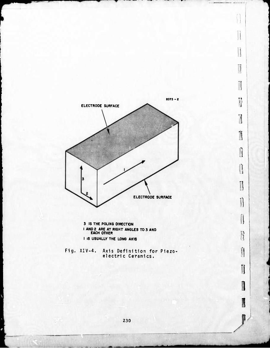
mm
i
t07S-t
ELECTRODE SURFACE
ELECTRODE SURFACE
3 IS THE POLING DIRECTION
I AND 2 ARE AT RIGHT ANGLES TO 3 AND EACH OTHER
I IS USUALLY THE LONG AXIS
Fig. XIV-4. Axis Definition for Piezo- electric Ceramics.
230
1
Q
1
II
II 1
X
J ^^^

▼~ iW*
I I 1 T I I
I
f
r r
i i
SECTION XIV
TABLE XIV-I
Piezoelectric Symbol Definition
r «33
ti
indicates that all stresses are constant, for example, zero
indicates that the electrodes are along the 3-3 axis
indicates that the modulus is measured with the electrodes shorted
free dielectr.c constant along the poled axis
11
«3?
indicates that the stress or strain is along the 1-1 axis
indicates that the applied stress or piezoelectric induced strain is in the 1-1 direction
.indicates that the electrodes are along the 3-3 axis
short circuit modulus of elasticity (Youngs Modulus)
piezoelectric voltage con- stant with all stresses, other than the stress involved in the second sub- script, are held constant
9 15
indicates that the stress or piezoelectric induced strain is ir shear form around the 2-2 axis
indicates that the electrodes are perpendicular to the 1-1 axis
piezoelectric shear stress constant with all stresses, other than the stress involved in the second sub- script, are held constant
temperature coefficient of linear expansion along the 1-1 axis
temperature coefficient of linear expansion along the 3-3 axis
3 density in k /m
1
i 12 = dielectric constant of free space = 8. 85 x 10 F/m
T836
231
*^ mm M

■»
The tension stress along the 1-1 axis is
12Mo o - s- z
w tJ
and the average stress across the thickness of one slab t/2 is
3M 5 = ^ (4)
The average field along z is
F = E/(t/2) (5)
From (3), (4) and (5)
3 :31M E = - —- ^. for one slab.
232
SECTION XIV
2. Output Voltage Equations ;
If two slabs of poled piezoelectric material are provided with
electrodes and rigidly fastened together as shown in Fig. XIV-5(a),
they form a bender transducer. The output voltage per unit input
moment can be calculated as follows: The reference axes are shown
in Fig. XIV-5(b). It is apparent that the upper half of the beam is in
tension and the lower half in compression and these strains have
mirror-image symmetry. Thus, the output voltage can be calculated ~|
for one-half and the result douoled ;;o find the total. I
As seen in Fig. XIV-5(b), the stress does not vary along x or y,
but only along z. Thus eq. (1) can be written
average field along z ,_. 831 average tension stress in the 1-1 axis '
1
\
D :l
§
e
i i
- }
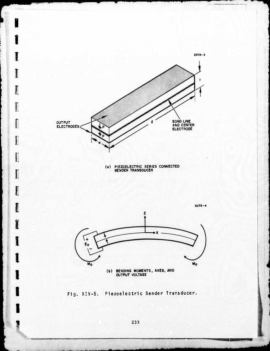
I
■•■■•"
2078-3
OUTPUT ELECTRODES
J 30ND LINE AND CENTER ELECTRODE
(o) PIEZOELECTRIC SERIES CONNECTED BENDER TRANSDUCER
(b) BENDING MOMENTS, AXES, AND OUTPUT VOLTAGE
8079-4
Fig. XIV-5. Piezoelectric Bender Transducer.
233
rfi^M ^■■■ftBHMBMMi

SECTION XIV
For the poling directions shown, the two slabs must be connected in
series and the total output voltage for a series connected pure bender
is
3g31Mo (6) wt
Since the g^, coefficient for these materials is inherently negative, the
output voltage will have the polarity shown in Fig. XIV-5(b), In many
elementary texts and examples the absolute value for g31 is used and
the minus sign omitted. This can lead to considerable confusion.
Because each transducer slab is sensitive to tension and com-
pression, it is necessary to evaluate the output due to a longitudinal
load. This output voltage sensitivity can be derived by the same
method as that used for the bending sensitivity, or it can be found in
any of the standard references, and it is
"83! w for tension (7)
where
P = force in Newtons
w = width in meters
This sensitivity is significant, but note that it is exactly canceled by
an equal and opposite voltage from the other slab, because for longi-
tudinal loads both slabs are either in tension or compression. Thus,
to first order, the bender transducer is not sensitive to longitudinal
loading. If one end of the clamped transducer is displaced as shown in
Fig. XIV-6, it is seen from the diagram that the average moment in
the transducer is zero. Because eq. (6) is exact for any element of
234
11 1
I
.1 1 1 1
"1
0 n 1 1 1
)
i^^fc-y

I
2078-8
I
M2 +
MOMENT DIAGRAM
- M,
I I
1 t I I I
I 1
Vz
SHEAR DIAGRAM
IT V|
Fig. XIV-6. Moment and Shear Diagram for One Type of Trans- ducer Loadi ng.
235

SECTION XIV
length, it is exact for a differential length. Thus, for the beam as a
whole, it represents the average moment over the length of the beam.
In view of this, it is concluded that the transducer sensitivity to the
type of bending shown in Fig. XIV-6 is zero. However, if M. is not
exactly equal to M?, then the.transducer acts as an end-loaded cantilever
beam and will have a significant output. This requires careful attention
to the transducer standoffs and clamps, which are discussed in a later
section.
In addition to the moment, the transducer is also subjected to
shear as s" own in Fig. XIV-6. From Table XIV-1 it is evident that
the voltage due to shear developed on an elemental transducer length
will have the form
e shear K g 15
The exact equation for transverse shear is
P g e shear 15
w (8)
on each slab where P is the shear force. The shear force in the two
slabs is constant and equal th'-oughout the active length of the slab.
However, due to the opposite poling direction in the two slabs, the
induced shear voltages cancel one another. Thus, the shear loading
sensitivity is also zero by first-order analysis.
Another possible loading condition of the transducer is shown
in Fig. XIV-7. This condition will arise when ♦•he sensors are mounted
with the spin axis horizontal and the transducer is subjected to the
gravity field. In this case, it is not self-evident that the average
moment in the transducer is zero, and the moment equation must be
written. It is
M = i W X - 1 l )
236
1
1
H
1
1
1
i
D !
B
n
i -—^ tmt^mam

r
r n D
W:wL
tttttt msm 2075-6
*m LOADING DIAGRAM
M, M XI M2 Tl- ■! 0.211 L T
j__ MOMENT DIAGRAM
r SHEAR DIAGRAM
r
i i i
DEFLECTION DIAGRAM
Fig. XIV-7. Moment and Shear Diagram for Second Type of Trans- ducer Loading.
237
MM

■
SECTION XIV
where
M = moment at distance x from one end
W = weight of the active section of the transducer
i = active length of the transducer
The average moment is
M W P /-. X2 1 A , W " ^ Jo \x""r "6 ^ dx = TZI IX2 - X3 - £X
Thus, this loading does not introduce an extraneous signal to a first-
order estimate.
Finally, it is possible for one clamp to move along the Y direction
with respect to the other (in and out of the paper) in Fig. XIV-6. This
introduces a stress that is identified as the parallel shear mode and the
equations and conditions are exactly the same as for eq. (8).
To a first order, the transducer is not sensitive to extraneous
forces, moments, and shear.
3. Equivalent Circuits
It is shown in Refs. XIV-1, -2, and -3 that for low frequency
operation piezoelectric transducers can be represented with reasonable
accui acy by either of the two equivalent circuits shown in Fig. XIV-8.
Some of the important defining relationships are shown on the figure.
The symbols used on Fig. XIV-8 are defined in Table XIV-2. The
equations are developed as follows.
Piezoelectric transducers have a funamental coupling coefficient
that defines the electrical energy and mechanical energy relationships
in the transducer. For the bender transducer, this coefficient will
238
I l
il i
n o
i
I 8
;
)
^amk
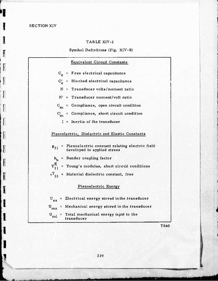
'I I
f
'
SECTION XIV
TABLE XIV-2
Symbol Definitions (Fig. XIV-8)
e
N
N'
C m
C m
I =
Equivalent Circuit Constants
Free electrical capacitance
Blocked electrical capacitance
Transducer volts/moment ratio
Transducer moment/volt ratio
Compliance, open circuit condition
Compliance, short circuit condition
Inertia of the transducer
Piezoelectric, Dielectric and Elastic Constants
^31
kb
YE
Ml = T • 33
U es
U ms
U mi
Piezoelectric constant relating electric field developed to applied stress
Bender coupling factor
Young's modulus, short circuit conditions
Material dielectric constant, free
Piezoelectric Energy
Electrical energy stored in the transducer
Mechanical energy stored in the transducer
Total mechanical energy input to the transducer
T840
239
-'V
._.^M*a^Ma

i SECTION XIV
£0TB-7
N : i
/TN0!" Mo = **« :c; V
V = NM oc o •3831M<
wt
N = 3g 31
wt
N'C m T (N1) C + C m e
N- =
N'C = NC m e
•E €T YE Wt •31 33 U
N'C = NC m e
kr = NN
m = N2C e + c m 12i ^m
Y^wt3 1 A Ce =
•33wi
t C e
'-^
1 1
m ♦ 5-y
6
NT' = »*ce (N')2( 3' N2C,
m e I c m m
2 T E 4 rf31€33Yll
Flg. XIV-8. Equivalent Circuits for Piezoelectric Bender Transducers with Interrelating Equations.
240
I
1 1 I 1 1 1 "I 1]
fl
fl
1
i
J J ^ma^A

I I I I I I c F. r i
i
i
i i i i ^
SECTION XIV
be designated as kb. The coefficient is defined by (I) for open circuit
renditions and a mechanical input.
2 Electrical energy stored in the transducer kb Mechanical energy input to the transducer
(1)
For an electrical input with the transducer free to move the equation
becomes
2 Mechanical energy stored in the transducer ^ b ~ Electrical energy input to the transducer
U < U
es U , - U - losses
mi ms U
(3) mi mi
neglecting losses
U ms U
(4) mi
It is apparent that if the electrical output of Fig. XIV-8(b) is short-
circuited, all of the transducer energy is stored in the short circuit
mechanical compliance, C'm, for a given input moment. Also, for
Fig. XIV-8(a) with the output open and a given input moment, all of the
input energy is stored in the open circuit mechanical compliance, Cm.
Since these circuits are fully reciprocal, when viewed from
the external terminals, and since the energy store is inversely pro-
portional to the compliances, we can write
U i
U ms
1/C m
mi 1/C m
C m C m
= 1 (5)
241

SECTION XIV
and
I
C =0' m m '-4 (6)
Using the value for N previously derived and the factors defined by the
physical constants, all of the relationships of Fig. XIV-8 can be
derived.
In the RGG sensor the moment of inertia of the transducer is
quite small and is included as a part of the arm inertia. The equivalent
piezoelectric transducer equivalent circuit for two series polarized
benders connected in parallel and connected to an RGG sensor is
shown in Fig. XIV-9. Note the change in use of symbol N in this
diagram to reduce the complexity of the working equations.
The Semiannual Technical Report No. 1 demonstrated the
method of relating the peak sensor stored energy to the peak electrical
stored energy of the transducer. Briefly
where
U mp
:zz Q
u
^eq
U mp (7)
= peak mechanical energy stored in the sensor com- pliances as a whole
= sensor arm inertia efficiency ratio = 0. 861
-3 2 = polar moment of inertia of one arm, 3. 561 x 10 kgm
= effective Q of the sensor including load resistor = 300
= sensor resonant frequency
-9 -2 = equivalent gravity gradient input = 10 sec
I 1 1 1 1 i 1 1
242
^tm^a

I I T
I r r r. r.
i i i i
1079- ■
If N : i -v^—|^-
= Hi
(k Co Voe
—»
Fig. XIV-9. RGG Sensor Equivalent Circuit.
243
M*. ^^-^m^^Bmam—mmm

^
SECTION XIV
and it was s hown that in the present nominal sensoi
U mp
21 2 1. 23 x 10 joules/^U
This energy will divide inversely as the pivot compliance. Cp. and the
open circuit mechanical compliance of the transducers, CJZ. That
is
U C, U _ , nip I
mi Cm/2 (8)
where
C = total system compliance
and
^2 p m
(9)
If we let the compliance r
then
atio of eq. (8) be a fixed fraction F,
F = c^2 = 0-1333
m
This is possible since C2 is fixed by the relationship
in one example
i. L,C. [CZZIZCZ] '
(10)
244
i
i
i
1
*m*^m*^^*im^mlä

^H
SECTION XIV
and C77/2 is fixed by the thermal noise limit.
The peak electrical energy stored in the transducer is
U = U .kj = U Fk^ = \c (V )2
es mi b mp b 2 ov oc (ID
Since
C = K.^ o 1 t
oc 2 wt
U es K
3 .3 wt
where the K, ... K- are constants. Since U is fixed, then only cer- 13 es tain values of C and V can be used. One procedure used to deter- o oc r
mine acceptable values of C and V is to plot the available values of r o oc C and V for a given U . Select a desirable combination of these oc ° es two and calculate the values for u, i and t that are determined by this
combination. If the resulting transducer is poorly proportioned, move
to a different combination of C and V that will alter the proportions o oc in a favorable direction. This is repeated until a satisfactory combina-
tion of parameters is obtained.
4. Transducer Computer Program
The relationships of the previous section can be applied in a
different manner. Select reasonable values for w, £ and t for the
individual transducers and then calculate, Co, Cj^/2» C,m/2» N' F and
C . If these values are satisfactory the designer can then calculate p
the pivot dimensions. If not, the transducer dimensions must be
' 245

VW*
i
SECTION XIV
adjusted within the constraints described in the preceding paragraphs
and new calculations made.
Once satisfactory transducer dimensions have been established,
the designer can calculate the pivot dimensions by the method described
in the Semiannual Technical Report No. 1. Note that the pivot dimen-
sions can be calculated as long as some compliance ratio is established
between the end pivots and the differential pivots. Also a length-to-
diameter ratio must be established for each type of pivot. The simplest
preliminary assumption is to assume that all pivots have equal compli-
ance and a length-to-diameter ratio of one.
All of the terms relating to the transducers and pivots have
been combined into the simple computer program shown in Fig. XIV-10.
This program uses the basic piezoelectric material characteristics,
assumed transducer dimensions and pivot material shear modulus.
The program calculates all of the transducer parameters and the pivot
dimensions. The calculated parameters are then used in the sensor
computer program previously given to calculate the sensor frequency,
signal level, and phase response of the sensor as a whole.
5. Transducer Specification
Two identical series polarized piezoelectric bender transducers
will be used on each RGG sensor. The dimensions of each transducer
are shown in Fig, XIV-11. The outputs of the two transducers will
be connected in parallel. These dimensions, with the material
characteristics, provide the transducer characteristics that have been
used in the previous paragraphs of this section.
The transducers will be operated in an evacuated chamber
{~10 mm Hg) at a temperature of 55 ±0. 01oC. The set point (550C)
may differ by ±5 C in the final device, but the temperature excursions
will be maintained to ±0. 01oC or better. In the nonoperating condition,
the transducers will be subjected to temperatures between 5 and 70OC.
The piezoelectric material characteristics and the character-
istics of the fabricated bender are shown in Table XIV-3. The material
246
I I 1 1 1 I I 1 1 1
1 1 1 1 I I 1
J ^*m ^^^1

"
1
I
i I r i i
i ^
100 REH 110 REN 120 REM 130 REN 140 REN 190 REN ISO REN 170 REN ISO REN 190 REN 200 REN 210 REN 220 REN 250 REN 240 REN 290 REN 260 REN 270 REN 280 REN 290 REN 300 REN 310 REN 320 REN 330 REN 340 LET 390 LET 360 LET 370 LET 380 LET 390 LET 400 LET 410 LET 420 LET 430 LET 440 LET 490 LET 460 LET 470 LET 480 LET 490 LET 900 LET 910 LET 920 LET 930 PRI 940 PRI 990 PRI 960 PRI 970 PRI 980 PRI
PRBQRAN WANE xTD-1" _ ■ m mmmmmmm m»mm m^mmm
THIS PRBGRAN CALCULATES THE PIEZO XDR COEFFICIEMTS 8F TWO SERIES POLARIZED PURE BENDER BINORPHS CONNECTED IN PARALLEL. IT ALSO CALCULATES PIVOT L AND D. U3 : WIDTH OF XDR IN NETERS L3 = ACTIVE LENGTH IF XDR IN NETERS T3 s XDR THICKNESS I" NETERS ES : XDR FREE DIELECTRIC CONSTANT
S: 5SS ÄSI 8'KMr«.-cu., C«..T.K. CO = BUTPUT CAPACITY OF PARALLEL XORS
n; r.?jr^LPLsrEirFiE!i.rrN XSR INSF^;; ;ä« CC ! J^^Ü^HiNjSrJSSSlKcr F^JL^PSSBTS IN DIFF. NBDE So = USM«"» KTUIML SSUMCY IF SENSOR, 220 RAD/SEC
1/2 NONENT OF INERTIA OF ONE ARN , SHEAR NSDULUS OF PIVBTS, «;» l*W "J BE-CÜ- PIVOT LENGTH = PIVBT DIANETER, NETERS PIVBT DIAMETER IN INCHES _ mm »ArTTMN PEAK SENSBR ENERGY STBRED IN XDR nicTIM BF PEM IESSOR ENERGY STBRED IN PIVBTS 7.9E-3 2.94E-2 1.9E-3 l,9039E-e -IIE-3 6.3E10 4.9 E+10 220 1.78201816 E-3 2*E3*W«L3/T3*(1-3*G3T2*E3*Y3/4)
1 / U0t2 /LI •0.9 * 03 * E3 * Y3 * «3 * T3
CO • C2 / ( CO - C2 ♦ Nt2) 6*L3/Y3/W3/T3t3 Cl • C3 / ( C3 - Cl ) I - C2 /C9
990 END
LI G9 L9 D9 F3 F9 W3 L5 T3 E3 03 Y3 Q9 WO LI CO 02 N Cl C3 C9 F3 F9 L9 D9
NT "CO NT -02 NT "C9 NT "N NT "WO NT "D9
C2 / C9 ( 16 / 3 / 3.14199 / L9 / 2,94 E-2
CO, C2, C9 N , WO, D9
'Cl - "C3 s
"F3 :
Cl 03
F3
09 / C9 ) r(l/3)
"L*» = " L9
CO : C2 r C9 = N : WO : D9 -
3.49062 1.19942 1.33687 9.86083 220 9.96391
E-9 E-2 E-2 E-9
E-2
Cl = C3 s
F3 = L9 =
I.17281 E-2 9.99673 E-2
.132729 I.41313 E-3
Fig. XIV-IO. Piezoelectric Transducer Computations
247
^m ^^

■ ' ' •m • 'W r
2070-9
CLAMPING AREAS
ELECTRODE AREA BOTH SIDES
0.15
3.34 HT ALL DIMENSION IN CENTIMETERS
Fig. XIV-ll. Piezoelectric Bender Transducer, Series Polarized.
248
>
- - -^ ^^aammä^äm^mt^mm

!
I SECTION XIV
i
1
I
I
I I I
I 1
TABLE XIV-3
Piezoelectric Material Characteristics
Characteristics*
T R «33 = 1. 5035 x 10 ±10%
g31 = 11.00 x 10" ±10%
YJJ = 6. 3 x 10¹⁰ ±10%
P = 7.3 x 10 ±5%
O-
Qmech = 80 ±20%
11 Volume resistivity >10 ohm m
Variation with Temperature PPM/oc at 550C
+3215 ±10%
-1930 ±10%
+ 643 ±10%
+ 1.4 ±20%
+4. 0 ± 20%
Characteristics at 250C after 1000 hr storage at 550C. Alternatively these may be specified at 550C.
T841
is of a type known as lead-zirconate-titanate, but the exact composition
is unknown. One material of this type is known as PZT-5A, a trade-
mark of Vernitron Piezoelectric Division. The detailed characteristic?
of PZT-5A are well documented in Vernitron (formerly Clevite)
specification sheets and in the Ref. XIV-5.
Extreme values of dielectric constant, electromechanical
coupling coefficient, mechanical Q, and modulus of elasticity are not
required. These coefficients may vary slowly with age since we expect
249
*m*^

SECTION XIV
to recalibrate the sensor as a whole every 10 to 100 hours. However,
the smaller the coefficient variation with time the easier it will be to' use the sensor.
After the transducers are received by Hughes they will be oven-
aged at 550C in a stress-free, short circuit condition for 5 weeks prior
to installation in the sensor. Applied voltages during testing will never exceed 100 V/cm.
It is shown in Section XIV-D that the variations with temperature
allowed in the table, the transducer variations, have little influence on the temperature sensitivity of the sensor as a whole.
1 I 1 i 1
250
)
/
• - ■■ ««MM

SECTION XTV
I 1
D. SENSOR THERMAL SENSITIVITY
It was shown in Section XIV-A that the output voltage of the sensor.transducer system was
nr nr (R2+I2)1/2 Z (1)
and the phase was
4» = tan'M-I/R) (2)
when the rotation frequency was w. In equations (1) and (2)
Lj NLRoL! C^j ow J (3)
I(W) = Ü N
R.C ,
'1 Ro R L.C.co2
oil (4)
Taking the derivatives of (3) and (4) with respect to I and R for constant CJ , we have
•nr eq [ RdR f Idl L Z3/2 "
(5)
and
d«j> = IdR - Rdl (6)
251

SECTION XIV
From (2)
x R j . -I cos 9 = —■ and sin d> = — Z Y Z
Equation (5) can then be written as (7)
E E fdR cos <<) - dl sin 4>1 " o L Z J (7)
and multiplying (6) by (1) we have
d(|) = -E rdI C08 «*> + dR sin <t>1 (8)
Since the sensor will be operated at an w such that <j) is almost
exactly TT/2, we can evaluate (7) and (8) at this point. Any small devia-
tions in the operating frequency and thus small changes in <)> from this
value will not materially affect the analysis. Thus
d E E « o Z
d<j. = -E ^ o Z
(9)
(10)
Since these represent the trace (cos) and cross trace (sin) gradient
error terms, we can write directly
dr. zr
ij
dl Z (11)
252
I i i
I I
B fl
1 1 I fl
1 "I II §
1
«fli ^m* ^

I
r SECTION XIV
dr
ZPi dR
Z (12)
To find the temperature inauced gradient error sensitivity, the
partial derivatives of all the temperature-sensitive parameters for
R(OJ ) and I(w) must be evaluated for constant w. Since every parameter
is temperature -sensitive to some extent they will all be evaluated.
Also, since there are going to be many partials they will be assigned
alphanumeric symbols where possible. Taking R first,
9R N + N\R0 cj
dR _ 1 / 1 2\ 9C0 N^L, '* )
dR 4 BRj NRoLj
3R _ 1 1 9N Ll 'N2
|R
OL
1 C1L1
R, C x o t •- w
dR 5 9R o NR 2L1 o 1
dR
(t) o
NL 1
253
— -^ A^ta

SECTION XIV
Taking the partials of I,
B ' = a", = "Ljp)(RlCo'R0clU2)
B
E.
91 wRj
2 9C0 NL!
9.- s w
N2
rRico+1 i (3 9N hi Ro ' R^C^2
B
91
91
w1
NL,
u 5 9Rr NR'1 LJCJW'
B, 91 1
^)
NR^Liw o^l'
We can now write the errcr derivatives due to the derivatives
of the parameters
dr
zr £_ - J. ij| " Z
BjdLj +B2dCo + B3dN + B^Rj +B5dRo +B6d (*)]""
264
f]
I
I
1 1 1 1 1 n
H 1
0 fl !i II
J

Ml
SLCTIüN XIV
dr
zr U AldLl +A2dCo + A3dN +A4dRl + A5dRo + V^) (14)
1 i
The temperature partials of the parameter derivatives must
now be evaluated at their operating temperature. The temperature
differentials may not be the same for all of the elements so provision
will be made to account for this
dL. = i-dT, 1 9T! 1
(15)
dC 9C —2dT, 9T2 2
(16)
[ dN = -^idT? 9T, 2 (17)
dR, 9R, LdT, 9T^ 3
(18)
dR 9R
9T4 4 (19)
ft) 9TC 5 9T?
dT. (20)
255
■«M^te mmtmmtä^^ mam

■ " 'P'
SECTION XIV
In the above equations the referred temperature differentials
are as follows:
dT. — arms
dT^ — transducer
dT, — arm-pivot loss term
dT. — preamplifier
dTg — pivots
The individual temperature partials are evaluated as follows:
L. is of the form
h = -H2 (21)
where
m = masp of the arm
k = radius of gyration, a linear function of temperature
9T, Z dTi (22)
1
The linear temperature expansion coefficient of the arm is a& and a& is
defined
if) dT a
(23)
256
1
I
i
i
0 i
0
i
0 I
!1 II I II 11
J 1^t^—^m*

^ ■V
I I SECTION XIV
or
1
I I
and
9T ko (24)
9L1 2 — = mk aa = 2L1aa (25)
dL, ZL.o dT. I a 1 (26)
1 The temperature-sensitive partials of C are quite complex
unless a simplifying assumption is made. The equation for C can be
written as shown in previous sections
2t33^ (27)
The kb term is small and does not vary greatly with temperature. In
addition the dCo terms are small as can be seeu on the computer print-
out (Fig. XIV-12). Therefore, it is satisfactory to assume k? is con-
slant in this particular case. Following the same procedure used to
evaluate dL,, we have for dC i o
dC = C Qv, + 0rQt +
dt. 33
33
/9T. dT. (28)
1 1 257
~ - mimmtmtcma^ MMftM

11 I
PAR-1
100 RCN 110 REM 120 REM 130 REM 140 REH 190 REH 160 REM 170 REM 180 REM 190 REM 200 REM 210 REM 220 REM 230 REM 240 REM 290 REM 260 REM 270 REM 280 REM 290 REM 300 REM 310 REM 320 REM 330 REM 340 REM 390 REM 360 REM 370 REM 380 REM 390 REM 400 REM 410 REN 420 REM 430 REM 440 REM 490 REN 460 REN 470 REN 480 REN 490 REN 900 REN 910 REN 920 REN 930 REN 940 REN 990 REN 960 REN 970 REN 980 REN 990 REN
PR0GRAN NANE PAR-I - " mmmmmmmmmmmmmmmmmm "
THIS PR0GRAN CALCULATES THE GRAVITY GRADIENT ERRORS IN THE SIN AND C3S CHANNELS DUE TO THE THERHAL SENSITIVITY OF THE SENSOR AND TRANSDUCER. THIS PROGRAM ASSUMES A HORIZONTAL SPIN AXIS SENSOR AND 2 6ANNA SUB IJ : 4900 EU.
04 = THERM. PARTIAL OF XDR 051 E4 r THERM, PARTIAL OF XDR E33 SUPER T Y4 s THERM, PARTIAL OF XDR Yl I SUPER E P2 s THERM, PARTIAL OF XD«? ALPHA, THICKNESS P3 = THERM. PARTIAL OF XDR ALPHA, WIDTH P4 = THERM, PARTIAL OF XDR ALPHA, LENGTH PI = THERM, PARTIAL OF ARMS, ALPHA, LENGTH AND WISTH P9 = THERM, PARTIAL OF PIVOTS, ALPHA, LENGTH AND WIDTH P6 = THERM. PARTIAL OF BRACE, M.PHA, LENGTH AND WIDTH 01 = THERM, PARTIAL OF PIVOT SHEAR MODULUS Hi. r THERM, PARTIAL OF Rl, ARN NECH, DANPING R9 s THERN, PARTIAL OF RO, OUTPUT LOAD RESISTOR
ALL THERN, PARTIALS 04,E4 R9, APE IN PPN /DEQ C Tl s DELTA TENP, CHANGE fcF ARNS, DEQ C T2 t DELTA TENP, CHANGE OF XDR, DE6 C T6 = DELTA TEM*. CHANGE OF Rl, DEG C T4 : DELTA TENP, CHANGE OF RO, DEQ C T9 s DELTA TENP. CHANQE OF PIVOTS, DEQ C
ARMS • 6061 ALUNINUN Y s 6.8 E+10 ALPHA r 23.4
PIV3TS • BERYLLIUN COPPER G9 t 4,9 E+10 ALPHA : P9 = •»•16,6 61 t -330
BRACE FOP PIVOT BRACE PLATE • 606! ALUNINUN Y : 6,8 E+10 ALPHA : «-23,4
TRANSDUCER - PZT 9-A AT 99 DEG C "PIEZOELECTRIC TRANSDUCER NATERIALS" .'AFFE AND BERLINCOURT IEEE, VOL 93, NO 10, (OCT IS69 ), 1372*1386
031 = 03 = -9,9 E-3 Yll SUPER E = Y3 r 6,17016 E+10 E33 SUPER T = E3 r 1,6819 E-8
Fig. XIV-12. Computer Program to Evaluate RGG Sensor Temperature Sensitivity.
258
i
I
I
D I
I
I
I
II
Ö
1
J

M
I 1 I
PAR-1 CONTINUED
I
I
600 REM 610 REM S29 REM 630 REM 640 REM Q5 6)0 REN Q6 660 REN OS 670 REN E3 680 REH Y3 690 REN G9 700 REM 710 REM 720 HEN 750 REM
I
051 PARTIAL = 04 = -1.9289 E+3 Yll PARTIAL s Y4 s +643 E55 PARTIAL I 14 t 3214.8
s SIN CHANNEL QPAV. O'AP. !N EU ( PHASE ERR3R) s C0S CHANNEL QRAV. 6RAD. TU EU < AMPLITUDE ERROR ) s -9.5 E-3 ? 1.6815 E-8 = 6.17016 E 10 mmmm s PIVaT SHEAR N^PULUS, 4.5 E+10 BERYLL1UN C0PPER ALL DATA AND CaEFFIClENTS MUST BE AT THE «TLRATINQ TEMPERATURE s 326K = 53C s 127.6 F DATAt Tl, T2, T6, T4, T5, MUST BE IN THIS ORDER,
IN DEG C, «NP NUST CARRY C0RELLATED SIGNS. 740 DATA ♦.OOI, -»-.OOI, +.001, +.001, +.001 75f READ Tl, T2, T6, T4, T5 760 LET 04 « -1.9289 E 3 770 LET E4 I 3214.8 780 LEf Y4 = +643 790 LET P2 = -M 800 LET P3 : +1.4 810 LET P4 s +1.4 820 LET PI ■ +20 830 LET P5 : + 16.6 840 LET P6 = + 23.4 850 LET 01 I -330 SCO LET R2 I -»-SO 870 LET R5 : + 40 880 LET CO : 3.49 E-9 890 LET Cl l 1.1730459 E-2 90« LET LI s 1.78201816 E-3 910 LET R« = 9.55 E+6 920 LET Rl a 6.1165552 E-4 930 LET N « 5.912 E-5 940 LET W s 219.98 950 LET R = N/LI •»■ 1/N*( R1/R0/L1 + C0/CI/L1 -C0*Wt2) 960 LET I = W/N ♦ < RI*C0/L1 + i/RO - I/R0/LI/Cl/Wt2 ) 970 LET Z s ( Rt2 + It2 )t.5 980 LET C3 s 9.55673 E-2 990 LET C9 : Cl * C3 / ( C3 - Cl > 1000 LET 12 s 4500 E-6 / Z 1010 LET Al = -I/Llt2 * ( N + (Rl/RO + CO/CD/N ) 1020 LET A8 = (1/Cl/Ll-Wt2)/N 1030 LET A3 = 1/L1 - <P1/P0/L1 + C0/CI/L1 - CO ♦ Wt2)/Nt2 1040 LET A4 t 1/N/R0/L1 1050 LET A5 = -Rl/N/r0t2/Ll 1060 LET A6 : CO / N / LI 1070 PRINT •• R = " R 1080 PRINT - I s " I 1090 PRINT " Z s - Z
I Fig. XIV-12. Continued.
} 259
mm
^m*

PAR-I C0NTINUED
MOO 1110 1120 1130 1140 1190 1160 1170 1180 1190 1200 1210 122« 1230 1240 1290 1260 1270 1280 1290 1300 1310 1320 1330 1340 1390 1360 1370 1380 1390 1400 1410 1420 1430 1440 1490 M60 1470 1480 1490
PRIMT PRINT LET Bl LET B2 LET 83 LET B4 LET B5 LET B6 LET Kf LET K2 LET K3 LET K4 LET K9 LET K6 LET K7 LET Ml LET M2 LET M3 LET N4 LET M9 LET H6 LET M7 PR1IIT • PRINT ' PRINT ' PRINT " PRINT PRINT • PRINf ' PRINT ' PRINT " LET 0? LET 09 LET 06 LET 06 PRINT PRINT ' PRINT PRINT ' END
-I/LlT2*W/N*m*C0-l/R0/CI/WtC) V*R1/N/L1 -¥/Nt2*(RI«C0/LI +I/R0-1/P0/Ll/Cl/Wt2) »*C0/I»/L1 -W/H/R0t2*(l-l/LI/Cl/Wt2) -l/N/RO/Ll/W
: Z2 : Z2 : Z2 : Z2 : Z2 : Z2 : Z2 : Z2 : Z2 i Z2 : Z2 : Z2 : Z2 : Z2 Kl t K3 : K9 : K7 s
Al A2 AS A4 A3 A6 A6 Bl B2 B3 B4 B9 B6 B6
LI CO N Rl RO 69 C3 LI CO N Rl RO 09 es
Kl, "K2 I KS, "K4 s K5, "K6 = K7
TI T2 T2 T6 T4 T9 T2 Tl T2 T2 T6 T4 T9 T2
K2 K4 X6
Ml = " HI, "H2 = " M2 H3 s " H3, "M4 = " M4 H9 s - M9, "M« s " MS H7 s - M7
: KI*2*PI 4 K2*(P3+P<-P2+E4) + K3*(P3+P4+04+Y4) + K4*R2 : 09 ♦ K9*R5 + X6*(6*(P9-P6H3*P9«>0I) "»• K7*<P3*P2-P4*Y4) s M1*2*P1 + M2*(P3+P4-P2+E4> •fM3*(P34-P44-Q4-fE44>Y4) ♦ H4*lt2 : 06 -f M9*R5 ♦ I16«(6*(P9-P6H3*P94'Q1) -f M7*<P34P2-P44-Y4)
09 = " 09
Q6 : " 06
Fig. XIV-12. Continued.
260
I
i
I
i
I
i
I
i
i
ii
■i
J /
-r-
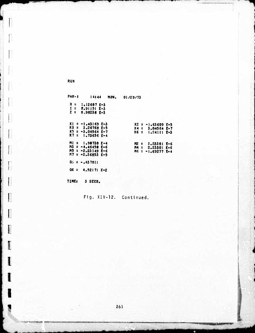
■^
I
RUN
PAR-I 14144 M0N, 01/29/73
R s I = Z =
1.12607 E-3 8.91191 E-3 8,98238 E-3
Kl s K3 = K5 = K7 r
-1.43169 E-3 5.28768 E-9
-3.04964 E-7 1.73696 E-4
Ml s M3 : M9 = (17 =
1.90730 E-4 -4.46490 E-6 -2.23149 E-6 -2.36893 E-9
G-, 8 -.437811
06 • 4.92171 E-2
K2 X4 K6
M2 114 MS
•1.63609 E-9 3.04964 E-7 1.24111 E-3
2.23301 E-6 2.23301 E-6
'1.69277 E-4
TINEt 3 SECS.
Fig. XIV-12. Continued.
261
(MMWMMMMMMVMfl
MMa-MtflMtaBflBlaMl

SECTION XIV
!
where:
a-w
or, —
«x —
linear temperature coefficient of expansion of the transducer width
linear temperature coefficient of expansion of the transducer length
linear temperature coefficient of expansion of the transducer thickness
'di — ]/dT? temperature coefficient of the transducer
dielectric constant
The above coefficients are tabulated in the transducer specification.
The equation for N, the transducer transformation ratio is
N = -Jhi^n** (29)
T 1 1
The temperature sensitivity of its differential at the transducer tem-
perature T- is
dN = N a + o w .•&)
'di 33
33.
'dY
11
dT. (30)
Where o and a are as previously defined and the coefficient partial«
are from the transducer specification.
262
1
^mt^mm^amM

^r
i
I
i
i I
SECTION XIV
The temperature sensitivity of R,, the internal mechanical
damping of the sensor is simply the partial
dRj = Rj '8R,
I/9T, dT. (31)
It is estimated that this will be +50 parts per million per C.
The external load resistor will be selected for low temperature
coefficient, approximately +10 ppm/ C and its partial will be
dR = R o o .S/8T* dT (32)
The compliance derivative is made up of two parts as shown
in (33)
\C'; dM- +d (33)
in.
The pivot compliance, C , will be treated first. The defining equation
for cylindrical rods in torsion is
3TrD4G 16L
Kp (34)
I The factor of 3 appears in this equation because six identical pivots
make up the total pivot system as shown in the. Semiannual Technica)
Report No. 1. The equation is written in terms of D and i for the
individual pivots.
263
- — mmm

I SECTION XIV
Taking the stiffness partials
dKp =
and
dKp
8K 9K i-dD + SD 9£
di + !5 dG
dG
4K dD _£
D
Kpd£p KpdG
(35)
(36)
ill
l
The derivatives of D and H are senbitive to temperature due to
two effects. First, they have their normal coefficient of linear expan-
sion and second, they may be compressed or stretched by the pivot-arm
mounting structure. In the sensor the pivots are supported and
restrained by the central plate and the end plate (brace plate), which
in turn are held together by the braces. If the braces have a lower
thermal coefficient of expansion than the pivots, then the pivots will
be compressed anü shortened, and through Poisson's ratio their
diameter will be increased. It can be shown that for a simple structure
with one member tending to compress the other the compressive force
developed is
K - *P)*T (37)
where
compression force developed on the pivot
temperature coefficient of linear expansion of the brace
temperature coefficient of linear expansion of the pivot
264
1
1
1 !
fl
1
J *^i

T
[ r
SECTION XIV
A, , A = area of the brace and pivot respectr-ely
Y,,Y = Young's modulus of the brace and pivot b p i.i i r respectively'
The total elongation (contraction) of the pivot structure in this
case is found from
n Y A T- (38)
and
I
F i P P
YPAP
K - ttpKAT
ri +
YpAp>
Yb^by
(39)
or
de = dip = K- • -PK«
('
t YPAP\
(40)
D In eqs. (38) to (40) it is assumed that the active length of the
pivots, i , is relativelv fmall compared to the length of the brace. It
is further assumed that the active pivot area is so small that all of the
pivot compression takes place within the active pivot. There are
3 pivots associated with each brace length. Therefore the compression
of each individual pivot is
Up = i K - "P)'
(■' YpV YbAb.
dT (41)
265
^mM

^M
SECTION XIV
I .1
and the diameter of each individual pivot is increased due to Poisson's
ratio by
dD = -crdip
The total differential for D including both the force and the
direct temperature effect is
(42)
dD = i° dT aT
(0P " ^bjV + a D
Y_A_\ P 3/i+l£M \ YbAb/
dT
Similarly, for the pivot length
(43)
"1
i
1
1
dip = ^dT p aT .)«,
Y„A„\ P P 3(1 + \ YpAb/
dT (44)
Combining the appropriate terms and remembering that j?p = D,
we have
d(cp/ -p+(f) /8T dT,
266
(45)
1
0
1
1
H
1
J ^■ü

I
w
( SECTION XIV
Since the pivot area will be quite small compared to the area of the
brace and since fth/D ~ 9, eq. (44) can be approximated
'(t) • K b p (f)/-) dT (46)
I 1
Where
m/ 9T6 = temperature coefficient of pivot shear modulus
For the 2/C term we have m
m
Y*wt 6je (47)
for the two transducers, again taking the partiala and remembering that
this is a transducer term at a temperature T-
(t) mi o- + a. w t 9T2JdT2 (48)
I
The evaluation of the final temperature sensitivity is done best
in a simple computer program PAR-1, shown in Figure XIV-12. The
computer can not handle all of the subscripts and super scripts, so
alphanumeric symbols are assigned as shown in Table XIV.4. These
symbols are consistent with the other two computer programs shown in
this section, and all of the programs can be merged into a single pro- gram and run as a unit.
1 1 267
■■

»ti mmiJ
SECTION XIV
TABLE XIV.4
Conventional Symbols, Computer Symbols, and Definitions
co - CO
w = W3
1 = L3
t = T3
Cm/2 m r C3
N = N
E-,, = 03
m •31
9T2 = G4
blocked output capacitance of two trawsducers in parallel
width of each transducer
active length of each transducer
total thickness of each transducer
compliance of two transducers, short circuit
model transformation ratio
transducer field to stress piezoelectric constant
thermal sensitivity of g,.
33
11
= E3 = free dielectric constant of transducer
= E4 = thermal sensitivity of «_-
Y3 = modulus of elasticity of transducer
E = Y4 = thermal sensitivity of Y. .
o. = P2
a = P3 w
thermal expansion coefficient of transducer thickness
thermal expansion coefficient of transducer width
thermal expansion coefficient of transducer length
268
1 ] 1 I
i I i l
i
-__-r

^
I I ]
I 1
■
i. i:
i: I i i
i i 1
SECTION XIV
TABLE XIV-4
Conventional Symbols, Computer Symbols, and Definitions (Cont'd)
% = P6 = thermal expansion coefficient of brace
a a = PI = thermal expansion coefficient of arm
Q P
= P5 s thermal expansion coefficient of pivots
G P
= G9 = shear modulus of pivot material
/äGn\ / M \ pi /aT5 ■" Gl — temperature coefficient of G
Ll = Ll = 1 /2 the inertia of one arm
Cl = Cl = m°'-hanical compliance
CP = C9 = mechanical compliance of ail pivots,
differential mode
Z = Z = equivalent sensor impedance
Ro = RO = output load resistor
(SRo\ \Rol
/
/3T4 — R5 s temperature sensitivity of R u
Rl B Rl B internal mechanical damping
\Rl/
/ , /«S ~ R2 = temperature sensitivity of R.
arc = G6 = COS channel gradient error, Eu
ar8
= G5 s SIN channel gradient error, Eu
Note: All temperature per million/0C.
sensitive coefficients are given in parts
T842
269
VMHBI

^B ^1^ ■^
SECTION XIV
Finally, from eq. (13) and (14) and all of the derivatives, the
ental chang
changes, we have
incremental changes in F and F due to the incremental temperature c s
AF = c
2F. . x 10 i.l I
-6
B1L1(2aa)AT1
2 0 w i t 2
+ B,N(a + ot + G4 + E4 + Y4)AT, 3 w t 2
+ B4R1(R2)AT3 + B5R0(R5)AT4
+ B6C-(6(öp " V + 3ap + G1)AT5
+ B6^-^ +«t " «* + Y4^T2 C m
(49)
I I 1 1 T I 1 1
D and
AF 2F.. x 10"
I ^1 A1L1(2aa)AT1
+ A2C0(öw + ali-at+ E4)AT2
+ A,N(tt + or. + G4 + E4 + Y4)AT, 3 w t '2
+ A4R1(R2)AT3 + A5R0(R5)AT4
+ A6Ü-(6(ap " V + 3op + G1)AT5 P
+ A,-=-(o +«.-«.+ Y4)AT, 6 , w t I 2
m
270
(50)
1
1
B
■ mm *m*

r i
SECTION XIV
These are still far too complex to allow the important terms to
be easily recognized so the computer is programmed to print out the
zr. ij
equal coefficients for the temperature-sensitive partials for
4500 EU and all AT equal 0.001oC. The printouts are of the form shown
in (41) and (42)
I
AF = Kl(2o ) s a
+ K2(o + a. - a. + E4) w l t
+ K3(a h a. + G4 + E4 + Y4) w t
+ K4(R2)
+ K5(R5)
+ K6(6(o - ah) + la + Gl)
+ K7(a + a. - Q+ Y4) w t C (51)
and
AF = Ml(2o ) c a
+ UZ(a + Qt - au + E4) w ■ :
+ M3(a + a, + G4 + E4 + Y4) w t
+ M4(R2)
+ M5(R5)
+ M6(6(tt - a.) + 3o + Gl) P b p
+ M7(o +0.-0. + Y4) w t I
(52)
\
I I 1
In the printout, G5 = Ars, the phase error term, and G6 = AI^, the
amplitude error term. It is evident that the sensor phase error is
much more sensitive to temperature changes than the amplitude term.
This has been known generally since the original proposal but this
computer program provides a precise evaluation and comparison.
271
||_Ha-|aaM

SECTION XIV
E. TRANSDUCER MOUNTING STRUCTURE
0
I The computer printout evaluate J Arg = -0.438 EU for perfectly
correlated temperature d'fferentials of 0.001 0C at each point. This is
considered to be a worst-case situation. It is shown in Section XVIII,
Temperature Control Subsystem, that a temperature standard deviation
ofO.00114 C, and probably better can be attained in the sensor.
Adjusting the -VT's to this Vcilue gives a AF - -0.500 EU. This trans-
lates to a sensor phase error of 5.55 x lO"5 rad and a cr = 0,250 EU i
XY *1 standard deviation gradient error at the tensor element. In Section
IX-B, Phase Error Propagation hi the Rotating Gravity Gradometer,
sensor phase errors of 6 x 10"5 rad and (rxy = 0.27 were used in the
error analysis. Thus, it is expected the RGG prototype design will
have a slightly better phase error stability than is shown in the error analysis.
1
1 1.
The transducers are mounted as shown in th" layout of Section V.
Four posts are fixed on each arm, in a circle around the pivot, and
these posts extend through the brace plate and through the other arm
if the first arm is an inside arm. An axial view along the posts shows,
for both arms, the ends of eight posts arranged in a circle around the
pivot. A mounting plate is fixed to the four posts of one arm and
another plate to the four posts of the other arm. This arrangement is
shown in the layout. The transducer is then attached to the two mount- ing plates.
Each set of posts and mounting plate constitute a rigid isoelastic
structure that applies a pure bending moment to the end of each trans-
ducer. This stand-off structure is quite ripid in bending, torsion,
and to end loading. It is quite similar to the quadrilever pivot dis-
cussed in the original technical proposal.
Since the stand-off structures for each of the two arms will
have different length podts the diameter of these posts will have to be
designed so that the bending spring rates are equal. Also the mounting
plates and the transducer clamps will be designed so that they have both
static and dynamic mass balance about their longitudinal axis.
1
272
'

V
SECTION XV
ROTOR POWER SUBSYSTEM
The rotor power subsystem desciibed in the Semiannual
Technical Report No. 1, has been built and tested and performs as
predicted. Minor changes in component values were made to optimize
the regulation capability and temperature sensitivity. The prototype
design of the rotor power subsystem is shown in Fig. XV-1. The
packaging of this subsystem is included in Section XIX, along with all
of thu other rotor mounted electronics.
I
27 3
^äm

^^
l!
o I
S
E O)
■!->
(/) ^ (/) XI 3 to
k Ol 3 o D-
o +•» o a:
en
i
1 I
1 ]
274
o
i D
MM ^■t

I I 1 I
I (
I :
SECTION XVI
ROTOR SPEED CONTROL SUBSYSTEM
A. GENERAL
The rotor opeed control subsystem is comprised of an analog
spin motor servo, spin motor, tachometer, frequency reference and a
rotor-stator position pick-off. The position pick-off is also used in the
digital data reduction subsystem discussed in Section XXI. Although
the prototype design uses an analog spin motor servo it is expected
that the final design will use a digital servo and this will be tested
during Phase II. The following paragraphs discuss the subsystem
components and their performance in detail.
B. SPEED CONTROL SERVO
I 1 \
1 I I I
The "speed control servo" controls the frequency of the RGG
signal modulation process on the basis of the sampled phase error of
this process. The continuous phase error of the process is defined as
the difference between the actual position and the reference position of
the RGG rotating assembly as in (1), where a(t) is the actual, instan-
taneous angular velocity of the rotating assembly with respect to the
measurement reference frame of the case.
Mt) = / a(t)dt - wRt (1)
The sampled rhase error is taken as the value of (1) which exists at
the time of mechanical coincidence between rotor and stator reference
point? as described in paragraph E of this section.
'
27 5
- ritfMtaaMÜ

V •v^
SECTION XVI
Although the position error oC the speed control servo is sampled
and quantized, the remaining part of the servo proposed for the base-
line design is an analog mechanization employing proportional plus
integral control and ta-hometer feedback. A simplified functional
block diagram of the servo is shown in Fig. XVI-1. The upt.er portion
of Fig. XVI-1 depicts the tachometer feedback dynamics and the tachom-
eter measurement noise (Au,.). The lower portion of Fig. XVI-1
indicates the proportional plus integral control dynamics acting on the
sampled and held position error signal. The central portion of
Fig. XVI-1 represents the "plant dynamics" of the rotating assembly
and the "plant disturbances" which include the normalized torque dis-
turbances (Td/J) and the RGG c se angular velocity («c). The normal-
ized damping coefficient (D/J) of the plant is the combined effect of the
viscous damping of the spin bearing, the electromagnetic drag of the
motor and tachometer, and the windage effects of the rotating assembly.
The calculated damping coefficient for the baseline design is 1193 dem-sec
and the polar moment of inertia of the rotating assembly is estimated to
be 2. 5 x 10⁵ gm-cm2. These figures yield a normalized damping coeffi-
cient (D/J) equal to 0. 0048 sec"1 The constant input quantities repre-
sented in Fig. XVI-1 are the reference speed command, (wR), the
tachometer bias (t^), and the normalized average running torque (To/J).
The sample and hold operation on the position error may be
approximated as a simple, first-order lag (for Trequencies well below
the sampling frequency) with a time constant equal to one-half the sample
..me interval (Tg- yt\ In the baseline design, the sample frequency
is approximately 17. 5 Hz, and the servo position loop bandwidth is less
than 1 Hz. These conditions adequately satisfy the requirements for the
approximate representation of the sample and hold operation with a first
order lag of 28. 6 msec (corner freqiency = 35 rad/sec).
The tachometer feedback signal will be filtered by a first order
lag to reduce the effects of tachometer noise, and a notch filter will
be employed to reduce disturbances at twice the spin frequency. The
notch filter is not shown in Fig. XVI-1 because its gain and phase has
negligible effect within the servo bandwidth.
276
1
1
1
fl
i
i^^

I 1 1
G
Wh tOTB-M
4i wg D/J M '
10 (i+-^) r-^rz*
«—►*
Fig. XVI-1. Functional Block Diagram of Servo.
I
I 1
277
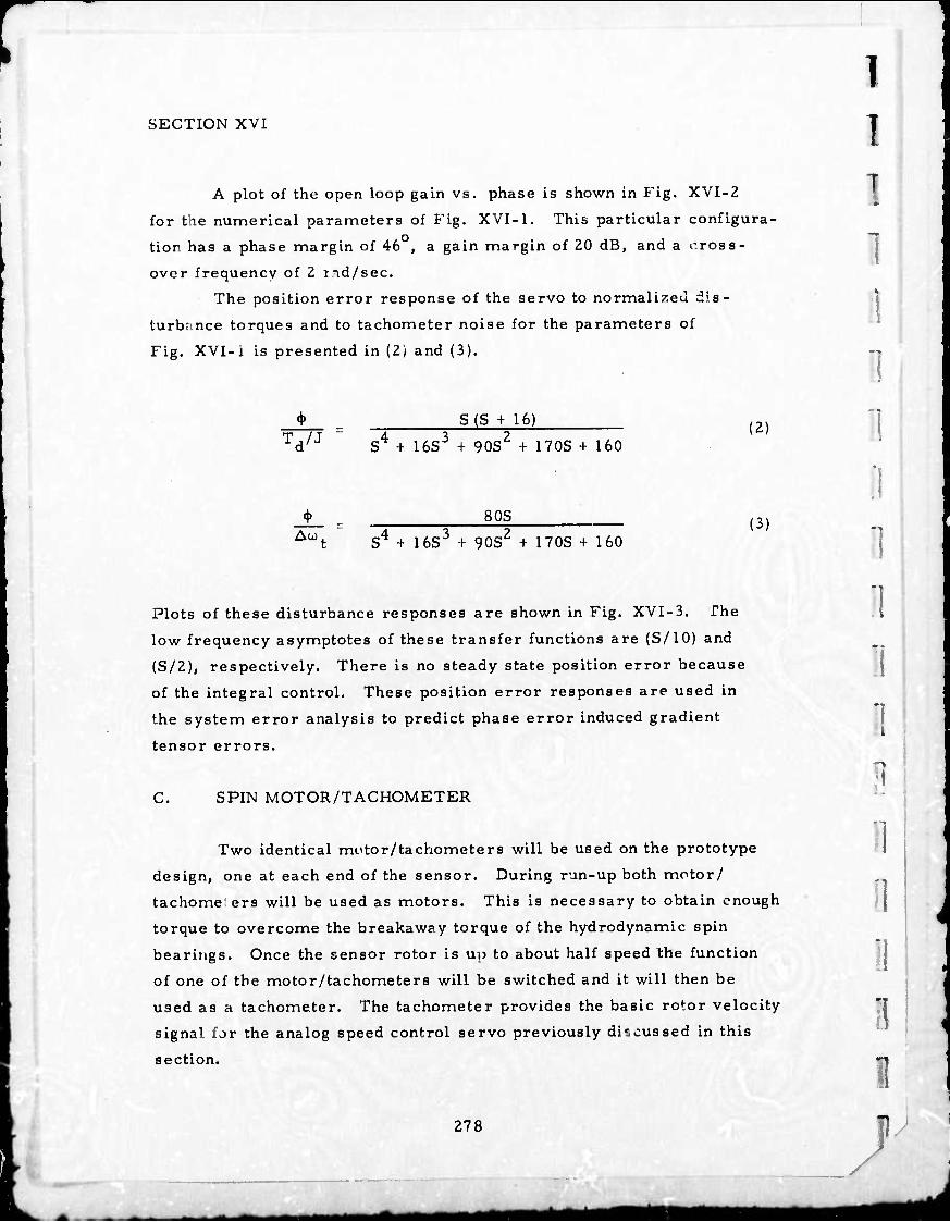
SECTION XVI
A plot of the open loop gain vs. phase is shown in Fig. XVI-2
for the numerical parameters of Fig. XVI-1. This particular configura-
tion has a phase margin of 46 , a gain margin of 20 dB, and a r.ross-
ovor frequency of 2 tnd/sec.
The position error response of the servo to normalized dis-
turbance torques and to tachometer noise for the parameters of
Fig. XVI-l is presented in (2) and (3).
1 I 1 1
* Td/J
AOJ,
S(S I- 16)
S4 + 16S3 + 90S2 + 170S + 160
80S
S4 + 16S3 + 90S2 + 170S + 160
(2)
(3)
.1
Plots of these disturbance responses are shown in Fig. XVI-3. The
low frequency asymptotes of these transfer functions are (S/10) and
(S/2), respectively. There is no steady state position error because
of the integral control. These position error responses are used in
the system error analysis to predict phase error induced gradient
tensor errors.
C. SPIN MOTOR/TACHOMETER
Two identical motor/tachometers will be used on the prototype
design, one at each end of the sensor. During run-up both motor/
tachometers will be used as motors. This is necessary to obtain enough
torque to overcome the breakaway torque of the hydrodynamic spin
bearings. Once the sensor rotor is up to about half speed the function
of one of the motor/tachometers will be switched and it will then be
used as a tachometer. The tachometer provides the basic rotor velocity
signal fjr the analog speed control servo previously discussed in this
section.
27 8
!i
i
I
J J
*Mrii mmm mam

I I I 1 I B r
i ]
\
i i i
20
10
< (9
S o o _l
UJ a. o
■10 -
-20
■zro
SPEED CONTROL SERVO
GAIN VS PHASE
PHASE MARGIN 46°
AT ui a 2 sec -'
GAIN MARGIN <f0 dB
AT<D S Msec-'
2079-29
■240 -210 -180 -150 OPEN LOOP PHASE, DEGREES
-120
I
i Fig. XVI-2. Speed Control Servo Gain Versus
Phase.
27 9
^tf^i

1.0
M
CD K 3 •- M 5
i rrfTTTi iorB-t4
I I I I I I ll[ I I—t < IM».
SPEED CONTROL SERVO ERROR RESPONSE
(TACH NOISE) 80S
SS ISS'+SOS^- I70S ♦ 160 I
0.01 J I I I III 1.0 10
FREQUENCY, rod/.tc 100
Fig. XVI-3. Speed Control Servo Error Response.
280
i
i
"i
1
"1 "(
fl
fl
i i 1 1
1
I - - - -- i l mik

I
I
I
i I 1 I
SECTION XVI
1. Motor/Tachometer Type Selection
Many types of motors and tachometers were considered for this
application. The requirements are in general:
a. Sufficient stall torque to overcome bearing friction.
b. Low and constant self generated ripple torque at operating speed.
c. Insensitive to external magnetic fields.
d. Lowest possible input power.
e. Good servo motor characteristics.
f. Good tachometer characteristics.
g. Size and form commensurate with the basic sensor design.
These requirements automatically exclude any motor that has
ferromagnetic material on the rotor. Ferromagnetic materials can not
be made sufficiently homogeneous to meet the ripple torque and external
magnetic field requirements. The requirements also exclude any motor
using brushes or '•ommutators. Only the drag cup servo motor can
meet the requirements. Its only drawback is that its efficiency is low,
about 10% at best. It can be used interchangeably as a motor or tachom-
eter although a good motor design is not necessarily a good tachometer
design.
Motor/tachometer specifications were sent to three motor design
consultants. These were;
R. H. Park, Co. , Inc. Main Street Brewster, Mass.
Herbert C. Rotors Associates, Inc. 45 North Mall Plainview, N. Y.
Philip H. Trickey 112 West Lavender Ave. Durham, N. C.
281
• - -

SECTION XVI
All of the consultants believed that they could design a motor that would
meet the specifications but only Mr. Trickey was equipped and had the
background to make the ripple torque calculations without farther study.
Mr. Trickey is semiretirc 1 after 30 years of designing drag cup motors
and tachometers. He is the author and coauthor of a number of classic
papers on the subject. Also he is a part-time professor at Duke Universiry
so that he has ready access to a large computer. Mr. Trickey was
selected to design the motcr/tachometer. The Spin Motor/Tachometer
specifications are reproduced as Appendix C.
i
Z. Description
The main motor parameters are given in Table XVI-1. The
motor is designed to operate at two different voltages. It operates at
62. 2 V on both phases to provide run-up and the breakaway torque of
the spin bearings. It operates at 37. 86 V on both phases in the speed
control servo mode.
Both the motor and Lie tachometer have a compensator winding
that is wound in parallel with the reference phase winding. The com-
pensator winding is of course electrically insulated from the reference
winding. The voltage induced in the compensator winding is a direct
measure of the magnetic field induced by the reference winding. The
output of the compensator winding will be fed back to control the
reference magnetic field to a constant value. This method of establish-
ing the reference field is commonly used with high precision resolvers
and is far superior to ether methods of establishing a constant reference
field.
Both the motor and the tachometer operate at a frequency of
140 Hz, which is locked to the basic frequency reference.
It is seen in Table XVI-1 that this is a "pancake" motor and is
similar in appearance to "pancake" resolvers in common use. The
Inner and outer stators are made exactly the same stack height so that
the inevitable fringing field at the gap is completely symmetrical.
282
fl
"I
"I
0 11
i
i
•^^^ mi

I r i i
I
I 1 1 I I I i
SECTION XVI
TABLE XVI-1
Spin Motor/Tachometer Characteristics
Motor
Phases 2 Poles 8 Frequency 140 Hz nominal Start-Up, Locked Rotor
Voltage 62.2 V Watts 30. 2 W
3.84 x 10b dem Torque Servo Mode at 1050 rpm
Voltage 37. 86 V Watts 9. 94 W
6. 69 x 10 dem Torque Compensator Winding Output 3. 78 V
Tachometer
Reference Phase at 1050 rpm Volts 20.8 V Watts 1.7 W
1. 11 x 10 dem Average Drag Compensator Winding Output 3. 78 V
Output at 1050 rpm Volts 1.42 V 7
1. 29 x 10" V/rad/sec Scale Factor
Dimensions
Stator - Outer Outside Dia. 4. 250 in. Inside Dia. 2. 875 in. Stack Height 0. 250 in. Winding Slots 32 Length Over-all 1. 00 in.
Stator — Inner Outside Dia. 2.791 in. Inside Dia. 2. 0 in. Stack Height 0. 250 in.
Drag Cup (Aluminum) Outside Dia. 2. 861 in. Inside Dia. 2. 791 in. Length 1. 00 in. Thickness 0. 035 in.
i
T870
283
^^^m 1 ' '
* m | '""

'W*'
SECTION XVI
The drag cup is made quite long so that the end effects are small and
predictable. These two latter features reduce both motor and tachom-
eter variations as the cup shifts with respect to the stators.
It is shown in Section IX-B, Phase Error Propagation in the
RGG, that a tachometer measurement noise of 10 rad/sec in a band
from 0 to 0. 1 Hz is all that is allowed to meet the rotor speed control
error budget. With the tachometer scale factor in Table XVI-1, tht
noise voltage is only 1.29 x 10" V. This is a formidable requirement,
but the noise band of importance is at very low frequency and the band is very narrow.
The tachometer output is at 140 Hz and can be easily amplified
with negligible noi^e and distortion to 14.2 V at 1050 rpm. This output
is phase sensitive, demodulated, filtered, and used in the rotor speed
control loop. The tachometer output voltage is at 140 Hz, and it inher-
ently has only the rotation speed, 17. 5 Hz, and its higher harmonics as
distortion terms. Note that the rotor speed and signal frequency are
harmonically related and phase locked by the use of one master refer-
ence frequency and a frequency synthesizer. The only means by which
a 0 to 0. 1 Hz signal can be generated is to modulate the tachometer out-
put voltage or phase by one of the following mechanisms:
Reference voltage modulation a.
b.
c.
d.
e.
f.
Translation of the drag cup with respect to the stator (axial, radial)
Resistance variation of the drag cup due to temperature variation
Stat. : iron loss change due to tsmperature variation
Stator permeability change due to temperature variation
Dimensional changes of stator and drag cup due to temperature variation
Thermal noise of the winding resistance component.
284
i
1
1
1
1
"1
!
0
■I
i 1
^Mta

■^
I I I 1 I
i I
I r
i i i
SECTION XVI
Although final design calculations have not been made, it is
believed that the tachometer will meet the noise voltage specification.
Other tachometers have been designed to perform with an accuracy of
Ü 1% over a range of ±10OC and with 0. 001 in. radial and axial rotor
play. Allowing for temperature variations at the motor of ±0. 1 C and -4 6 radial and axial play of 10 in. , this would scale to one part in 10 , a
little better than required. The actual temperature variation should be
less than ±0. 01OC and the radial and axial play will not exceed about
±10'5 in.
This tachometer has been designed with a compensator winding
and large drag cup overhang. Also, the output load will be a very high
resistance and can be temperature compensated. These features help
ensure that the tachometer will meet its specifications.
D. FREQUENCY REFERENCE
Two secondary standard frequency references are available.
Both of these are so accurate that the error due to the frequency
reference is negligible in the jrror analysis.
The Hewlett-Packard Mo. 10544A, 10 MHz Qua;tz Crystal
Oscillator, ages less than 5 x 10' per day, and less than 1.5x10 _9
per year. This oscillator warms up in 15 min to within 5x10 of the
final stabilized frequency. This same unit is incorporated as the clock
in all Hewlett-Packard frequency counters. One of these counters will
be used as a basic component of the prototype design.
The General Radio Type 1113-B, 5 MHz, Standard Frequency
Oscillator, ages less than 5 x 10' parts per day and less than -8 5 x 10" parts per year.
The General Radio Frequency Synthesizer is not quite as good as
the above two secondary standards but it is provided with terminals
that allows it to use an external frequency reference. The Hewlett-
Packard Frequency Counter will be used as the basic reference in the
Prototype Design. Its 10 MHz output will be used directly by the speed i
285
.,*- , -* «r*-/ 0 I

wmm
SECTION XVI
control servo, and the digital data reduction subsystem. In addition
the 10 MHz signal will be divided by two to obtain a 5 MHz reference
with an accuracy and stability equal to that of the reference. This
5 MHz will be used as the reference for the General Radio Frequency
Synthesizer. The Frequency Synthesizer will be used to provide thj
low frequency, 35 Hz locked to the standard, that is required by the
analog data reduction subsystem. This same Frequency Synthesizer
will also generate the 140 Hz required by the spin motor and tachometer.
The above combination of equipments will eliminate the frequency
reference as a significant source of error in the prototype design.
i
E. POSITION PICKOFF
A precision pickofi is required to detect coincidence, or the
error angle, of the rotor and stator reference points once each revolu-
tion. This will be accomplished in the prototype design by the use of a
pulsed light emitting diode (LED) as a light source, and a high speed
photocell to read the position of an encoder disc.
1. Requirements
The relative error between the rotor and stator must be detected
once each revolution with an instantaneous position uncertainty of no -5 more than 2. Z x 10 radians (1 sigma) and an average uncertainty of _5
no more than 2x10 radians (1 sigma). The mean position error will 7
be held to less than one part in 10 over periods of up to 10 hours by
means of the frequency reference previously discussed in paragraph D
of this section.
286
"i
1 1 1 1
i
I fl
"i 1 1
r ^rta *mk

I I I 1 r
I I
r i
SECTION XVI
The position error requirements, 1 sigma values, in
radians are
Reference frequency change
Center of rotation uncertainty due to "g" loads on bearing
1. 5 x 10'
1 x 10'
1 x 10 -5
1 x 10'
1 x 10
2 x 10'
-5
Sensor Arm Alignment to Rotor Case
Encoder Disk to Rotor Case
Photo Cell to Stator Alignment
RSS Alignment Variations, 1 sigma
The initial values of these terms are not important, except as a con-
venience, since they will all be calibrated prior to a test. It is only
their variation during a 3 to 10 hr test that are significant. The above
values are estimates, of course, but based on experience with optical
autocollimators, gyro and accelerometer pick-off stability and alignment
stability of precision devices in general, they are consideied to be
realistic. The long-term speed error (zero mean speed error) is met by
the use of the precision frequency reference previously described and
through the speed control servo forcing the average speed to equal the
set speed. The reference frequency is 107 Hz and the nominal speed
is 110 radians per second. The exact rotor speed for optimum per-
formance will be found by test and set to seven significant figures for
each sensor but the use of the nominal illustrates the technique.
A register is set in the computer that represents the number of
10 MHz counts that should occur during one revolution. This counter
is set to seven significant digits on a decimal base. A counter, that
counts the actual number of 10 MHz pulses during each revolution is
started and stopped by the re. erence slot on the encoder disk. This
actual count is compared with the ideal count and an error signal of the
proper polarity is generated and sent to the speed control servo. Thus
tne long time spe3d error is forced to zero. The counters just mentioned
'
287
M^MMi ^■^1

SECTION XVI
are clocked so that no bit of the 10 MHz count is ever lost. Thus even
if there should be exact coincidence between an encoder disk slot pulse
and a 10 MHz count, that count will be added to the count for the next
revolution.
The encoder disk is also used for digital data reduction which
is a considerably more complicated task than that just described. The
actual speed control counters and registers are incorporated within the
computer used for digital data reduction and the diagrams therefore
appear in Section XXI.
i
i
2. Encoder Disk
The encoder disk is glass and is opaque except for eight light
slots as shown in Fig. XVI-4. The reference slot is made significantly
wider than the others so that it can be identified by the computer.
At the pick-off point the encoder disk has a radius of 1. 625 in.
Rotating at 110 rad/'sec the slot velocity is
1 1 1
v = R u) = 179 inches per second s
(1)
The light source is focused to a spot 0. 001 in. in diameter at the slot.
Thus the light fall time ot. the photocell is
Fall Time = 10 R w
5. 6 x 10" sec
The photocell saturated level will be set to 10 V and the gate will be set _7
to 5 ±0. 2 V giving time resolution of 1. 1 x 10 sec and a position -5
resolution of 1. 2 x 10 rad. This will meet the pulse jitter require- -5 ment of 2. 2 x 10 radians previously stated as a requirement.
288
'I 1
51 ] 1 1
1
AJB *MÜ

I I 1 I
f.
1 1
'■
I I I 1 I I I I
DISC OPAQUE EXCEPT FOR SLOTS
2078-16
3.5 in.
REFERENCE SLOT
Fig. XVI-4. Encoder Disk
289
MB^Ma ^«M^HtflMi

SECTION XVI
1 For the single reference slot used for speed control, position
accuracy has no meaning since it is the reference. However as shown
in the figure there will be seven other slots on the disk. These slots
can be spaced and positioned to an accuracy of ±5 arc sec for a modest
cost disk. As shown in the section on digital data reduction, this
accuracy is entirely adequate. However, there is one other important
characterise f the placement cf these seven slots. They are placed
20 arc sec ah.ad of the exact one-eighth of a rotation position based on
the reference slot. The reason for this slot positioning is given in Section XXI.
Operation of the light source, photocell and encoder disk is as
follows: The light source is pulsed to high intensity just prior to the
leading edge of each slot and is extinguished immediately after the slot
has passed. This keeps the average dissipation of the LED to a low
level but provides a high intensity source at the time that it is needed
The computer can be programmed to turn the LED on and off at the
proper time. The computer also recognizes the reference slot by its
greater width and then keeps track of the other seven slots. When the
trailing edge of the slot passes through the light beam, the photocell
output goes to zero and this generates the position signal previously discussed.
1 1
1
■
290
1
I^M^i

mß w^^
I I I ]
l [
I B 1 1 [ l
l 1 I I
SECTION XVII
REMOTE ARM BALANCE SUBSYSTEM
The remote H.rm balance subsystem allows the mass balance of
the sensor arms to be adjusted while the sealed sensor is operating.
In addition the same logic system that controls the mass balance
adjustment provides a logic state that adjusts the gain of the signal
preamplifier and FM transmitter to provide "Normal" and "Low" gain
settings. The "Low" gain is used during initialization and coarse adjust-
ment. This same logic is also used to turn the sensor test signal on
and off. The subsystem diagram is shown in Fig. XVII-1. A discussion
of the packaging of the electronics of this subsystem is included in
Section XIX.
A. GENERAL
The arm balance subsystem consists of a power supply, the
same as that used for the sensor electronics, a logic section, a sequencer,
mass transport devices and three vibration drivers.
While the system is operating in a otatlc environment each of
the three vibration drivers will be excited in sequence to vibrate the
sensor along a known axis at a known amplitude. The phase and mag-
nitude of the change in the output signal will be measured and recorded.
The magnitude and direction of the mass shift required to correct the
differential mode arm mass unbalance will be calculated. By use of
the sequencer and logic the subsystem will be commanded to shift a
small precisely known mass a precisely known distance. It has been
shown in the Semiannual Technical Report No. 1 that the adjustment
can easily be made to one-hundredth the allowable residual unbalance.
The subsystem is essentially the same as previously described. It
has been refined in some areas.
291
rtk^MMM ^^^

E (U
>>
10
o
re CO
i. •a:
01 ■M O £ 0) a:
X
• en
•r- u.
_l ,-J o o s in 00 o O g i 2: f to o o z s 5 z CVJ
jl» ^ > * ■*- v
292
i
"I
1
1
"1
I
'I
1
i
i i
•I
n
y
MM ^^

t^mm
I I
SECTION XVII
The mass balance device logic commands are given by
interrupting the high voltage high frequency rotor power supply for
0. 1 ms = logic "l", 0. 3 ms = logic "0". The power supply, logic
sequencer, and balance logic have all been built and tested. They are
stable, do not generate false logic and drive the mass balance devices
as predicted.
I r
B. MASS TRANSPORT DEVICES
1. Requirements
It was shown in the Semiannual Technical Report No. 1 that the
mass balance devices were required to have a mass times distance
transport capability of
_4 Amh = ±56 x 10 gm cm/arm/axis
It must be possible to position the mass to an accuracy of
[ I I I I I
1
Amh ±4 x 10" gm cm
The mass balance devices have an inherent "g" limitation that must not
be exceeded. They must be capable of operating over the temperature
range anticipated for the sensor.
2. Description
The mass transport devices selected are small glass capillary
tubes, filled with mercury except for a small gap of electrolyte and a
gas pocket. A gas pocket, filled with dry nitrogen, will be left at the
293
*m*

SECTION XVII
"low g" end of the glass tube. This gas can absorb the expansion and
contraction of the mercury due to ambient temperature changes in the
non-operating condition. The tubes are sealed and provided with elec-
trodes at each end. When an electric current is passed between the
electrodes, mercury is plated from one side of the electrolyte gap to
the other and the gap is transported along the tube. The direction of
transport is controlled by the direction of the current, and the position
of the gap is proportional to the time integral of the current through the
balance device.
Devices similar to this have been described in a number of
patents and have been manufactured by Sprague Electric Co. ;
Plessey Inc. , Electrochemical Division (Formerly Bissett-Berman
Corp. ); and Curtis Instruments, Inc. Currently, Curtis Instruments
is in commercial production on a current integrator tube almost iden-
tical to the one required for the RGG sensor. Curtis has quoted, to
Hughes, a fixed price development and production contract for the
balance tubes that we will require, made to Hughes specification.
Hughes has (studied the literature and has decided that we could make
the balance tubes in our own laboratoriea. This would not be efficient,
due to learning problems, but it provides a backup source.
A drawing of the specified balance tube is shown in Fig. XVII-2.
A sketch of the mass balance device mounting arrangement is shown in
Fig. XVII-3. Ten tubes in series, in two groups of five each, will be
placed along each axis of each arm. The voltage drop across each
tube will be approximately 0. 15 V or a total of 1. 5 V at a current of
0. 5 mA. The electrolyte gap has an apparent negative mass of _4
7x10 g and a travel of ±0. 814 cm (±0. 32 in. ). Since there are ten
gaps on each axis the mass shift available is
n
!
1 1
\
0
0 i
I
I Amh ±57 x 10' g cm
as required by the previous paragraph. At a current of 0. 5 mA the gap
moves at P rate of 0. 254 cm (0. 1 in. ) per hour. Thus an end to end
294
I
i

I I I 1 I 1 1 I I I I I 1 1 I 1 I 1 1
1078-IE
MERCURY
ELECTROLYTE
DRY NITROGEN BUBBLE
Fig. XVII-2. Mass Balance Device
295
«M^H^^M*

I
ALUMINUM PLATE
tors-is
DRY NITROGEN BUBBLE
HUB TO ARM
Fig. XVII-3. Mass Balance Device Mounting.
296
I 1 1 I 1 1 I I I 1
i
■«■MM *MHMMril

!
SECTION XVII
' shift would require 6. 4 hr. It is evident that by timing the current
integration time, very fine resolution can be obtained.
The centrifugal acceleration near the pivot end (gas bubble end)
will be about 1 5 g. At the outer limit of gap travel, 1. 02 in. from the
center the acceleration will be 39 g. These are safely within the
theoretical and tested acceleration capability of over 60 g.
The device is completely satisfactory for the intended application.
3.
I i 1 I I
Specification
I
I
I
A condensed specification for the mass transport device is
given in Table XVII-1. In addition, the following inspections and tests
will be made:
a. Characteristics
Voltage drop
Travel range
Accuracy
Gap size
b. Environmental
Acceleration
Temperature cycle
c. Inspection
Gap size
X-ray for extraneous gas and gaps
Bubble size
Leak detection
Seals
I 1
297
• - '

SECTION XVII
TABLE XVII-1
Mass Balance Device Specification
Tube material
Tube fill material
1 in. lead
1 in. lead seal
1 in. lead Hg fill
Electrolyte
1 /2 in. lead
1/2 in. lead seal
1/2 lead end fill
Electrolyte gap size
Tube ID
Length overall (Leads bent 90°)
Max OD
Mass transport constant
Mass transport constant
Usable transport distance
C. VIBRATION DRIVER
Hard glass or quartz
Mercury
0. 008 in platinum
Glass to metal
<0. 50 mm Hg
Perchlorate (valence 1 with Hg)
0. 008 in platinum
Epoxy-room temp, cure
0.20 in. dry nitrogen bubble
0. 20 to 0. 23 in.
0. 15 in.
1. 00 in.
0. 60 in.
0. 1 in. /Hr at 0. 5 mA
Accuracy *2%
±0. 32 in.
T871
Three small vibration drivers will be mounted on orthogonal
axes of the RGG mounting platform. These are small commercially
available units that weigh 2 lb and can provide a force of 0. 5 lb at 10 W
298
I
"!
1
1
a i
•i i "i n
i 1
;
MfeaariMM

^M
I SECTION XVII
input power. This is sufficient force tu vibrate the sensor mounting _3
platform on the vibration isolation system to the 5x10 g level. This
is adequate to provide the excitation required to adjust the arm mass
unbalance.
D. SENSOR TEST SIGNAL
If an insulated plate is placed near some part of the sensor arm,
the plate and arm form a capacitor. If a voltage is applied to this plate
it will attract the arm with a force, F, acting at a lever arm, L. The
moment acting on the arm is
M. F L V2C L 2d
V"A £ L o_
2d2 (1)
where
M. = torque on the sensor arm, Nm t
V potential difference, volts
2 A = area of the plates, m
o
L
permittivity of free space, 8. 85 x 10
= lever arm, m
12
d = spacing between the arm and plate, m
The sensor design includes an insulated plate 1 cm square, with
a lever arm of 5 cm at the tip of each arm, which provides 4 capacitors.
Th^ voltage applied to each plr.te will be 10 volts, off of the rotor power
299
■■■■■

1 SECTION XVII
supply, the spacing will be 0. 1 cm and these capacitors will produce a
moment of
M = 8. 85 x 10"7 Nm
!
1 i
The sensor torque due to an input gravity gradient is
M = •nC T /2 = 1.533 x 10'11 Nm/EU (2) o ' zz eq
Thus the test capacitors can introduce a test gradient F which has
an effective value of
M, I\ = t 2M 228 EU (3)
1 1
The voltage required to excite the test capacitors will be
obtained from the Rotor Power Subsystem. The loading, due to test
capacitor excitation will be trivial, and it will be turned on and off with
the same logic circuitry and sequencer that are used to shift the mass
balance devices as previously described. These capacitors merely
provide an excitation voltage source that can be turned on or off by
external commands.
A 2GJ (=u ) frequency will be obtained inside the rotor by using so
two photocells on the rotor that are excited by a LED (light emitting
diode) mounted on the stator. These photocells will produce output
pulses at a frequency of co with their phase determined exactly by the
mechanical position of the sensor rotor with respect to the stator. The
photocell output pulses go to a single-shot multivibrator that has an
300
il 1
0
1
I 1^^ mmM

SECTION XVII
output pulse width of exactly 4IT/(JJ sec. The circuit and the wave forms
at various points are shown in Fig. XVII-4.
It is evident that a precisely phased and constant amplitude test
signal of approximately 228 EU can be introduced and removed by
external logic commands. The exact phase and amplitude are not
believed to be important. It is important that the phase nnd amplitude
remain constant over a reasonable period of time such as an hour. Due
to the temperature control and power supply regulation required by
other subsystems the stability of this test signal will easily meet all of
its requirements.
301

I
LIGHT IZt(pE) (PEJ SOURCE * V-/ V-X
+ 10 VOLTS
+ 10 VOLTS
©
ON-OFF LOGIC
2073-14
+ 10.0 VOLTS
ONE- SHOT MULTIVIBRATOR
ARM CAPACITORS
© 1111 T T T
SCHEMATIC DIAGRAM
2075-15
et 0)0
sec ^ 2» "o
WAVEFORM AT 0
i I
-»TIME
Wo 4» -♦TIME
Wo
WAVEFORM AT (b)
Fig. XVII-4. Test Signal Generator, Schematic and Waveforms.
302
1 1 I 1 1 1 1 1 D
1
I
1 1 1
MMMHto/

■S"
i
SECTION XVIII
TEMPERATURE CONTROL SUBSYSTEM
I 1 1 1 I \
I !
!
1 I I I I
A. TEMPERATURE CONTROL REQUIREMENTS ON CRITICAL COMPONENTS
There are two basic temperature requirements and an additional
dimensional stability requirement which establish the basic temperatuie
control parameters.
1. Analysis in Section XIV-D shows that the tempera- ture of the transducers must not drift greater than» ±10"^oC in order to maintain phase error signpl at u level well below 1 EU.
2. The bearing design requires a temperature stability at the oil film of the bearing within ±C. 03oC in order to maintain proper torque control on the drive system (see Section XII).
3. The bearing design also requires a dimensional stability of each oil film gap of ±5 \i in. or a total tolerance of ±10 \i in.
B. THERMAL MODEL
The thermal model chosen for this analysis consists of one or
two resistances for each basic part of the sensor. Since this analysis
is preliminary to the finalized design and finalized dimensions were
not known this level of detail appears realistic for a first cut at the
problem. It is expected that a more detailed analysis will be run dur-
ing the next phase of this program.
The thermal model chosen is shown in Fig. XVm-l(a). Here all
Y's are thermal conductances of individual components and the nodes
between the conductances represent the thermal masses of the com-
ponents. (Obviously some small mass components are considered to
have no thermal capacity).
303
M^a
MM

■p*
@ Wj @
TOP PIVOT
■5 «1;
\ 01« —•till
PIVOT PUTt
ItLECTKONICS
•X0
MEATtR POWER
.C»S£ \
Q4 MOTOK POWtV
CHI n-~^Tj
'•: 1 FILM
KMMO _. MI»T 06 (y
V4
1 «IB FILMITI*
i0BIM#ALHe*TJIN« i©
MICA * v ® IN5UUTOP5 f T'
^^r: «i!»
STATOP
AMBINT AIR
FILM1
®
(•)
T-'T
VV>A^-
1 T-l
Ml jZ
rite
_j^
Fig. XVIII-1. Thermal Model.
304
"hr 1
41
1 1 1 ]
1 I 1 1 1 1 B 1
i
1 1 1
J ----■*- ^^^

I I I !
I
I I I 1 I I I I
SECTION xvm
The principal heat inputs shown in Figure XVIII-l(b) are: »
Q3 — Heater Power (a parametric variable)
Q4 — Motor Power
Q6 — Friction loss in the bearing oil film
Q16 — Electronics Power
The computer program chosen to provide the thermal analysis
is the Hughes TAP-3 Thermal Analysis Program. The data was written
with a "bang-bang" heater function with a specified dead band, but could
easily be modified to a proportional controller type function. Thermal
runs were made assuming both a constant ambient environment, and
sinusoidally varying air temperature and gimbal heat sink temperature
(Tl and T17). Initial conditions were set at 70 F and a transient
analysis was run for each heater power level for the first 10 hr of
T operation. Readout was made of each node temperature each 0.02 hr
for the last 2 hr of each run.
Data for the program was as follows:
1. All thermal conductances and capacities are as listed in the -010 and -020 Data Sections and were not changed (see Fig. XVIII-2).
2. Heat Inputs
Q4- 1.7072 BTU/hr (Motor Power) Q6-0.751 BTU/hr (Bearing Losses) Q16 - 1. 366 BTU/hr (Electronics Power) Ti -0.250 sin (27rt)0F (Gimbal Temperature) T2 - 1. 000 sin (26. 8t) F (Air Temperature)
3. Sensor Operating Temperature
T = 135° and 90°
4. Heater Control Dead Band
±0. 001OF (±0. 01OF used in early runs)
305
**^^mmi^mm

«■
1
RUN NUMBER 1
ill NEW 1NPUT PAT* FOP THIS fill • 1 0 0 0, o,
THIS PPOOP** CALCUimS THE TH»NS;FNT IN THE DESIGN MODFL OF THE POTäTIMG G^.'VITV BEING DESIGNFn UNDF» COVTPtCT Fl'>615'72-
1 > 10
T3 HAS RhiCHEB CVtLIN J Iti-
NETWORK PESCPIPTIOK
1 14 0 o, o, 19 0 0 0.6J2910E 0^ 0,
16 0 0 o.eJsnooE co o. 17 0 0 r,769?3fiF OZ o, IS 0 0 0,405000E 00 o. 19 0 c o.essocoE oo o. ?0 0 0 0,57200CE-0l 0. ?1 0 0 o,7oeooPE oi o.
• 20 0 0 0, INITIAL VALUES
n.
T 2 1« 0 0,70P000E 02 n,
Y 1 0 0 0,1015006 m o. Y 2 0 0 0,699300E 02 0, v 3 0 0 0,285710E 02 n. y « 0 0 C.33333JE 03 o,
r 5 0 0 0,3413U0E 0? 0, v 6 0 0 Cl,341300E 02 0, Y 7 0 0 0,667(S0OE 01 o. Y 8 0 0 0,285710F 02 0, Y 9 0 0 0,716300E Cl 0. Y 10 0 0 0.62500nF 00 n. Y 11 0 0 0.414000E 00 0, Y 12 0 0 0,l44000E-02 o. Y 13 0 0 0,625000F CO o, Y H 0 0 0,«92«nOE 01 Di C 1 0 0 0. n. C 2 0 0 0,273600E CO o. C 3 0 0 O^SIOOOE 00 o, : 4 0 0 0,765400E 00 n. C 5 0 0 0, 0. e 6 0 0 0, 0. C 7 0 0 0,1860006 00 n. C 8 0 0 o,251oonF on 0. : 9 0 0 0,7300C0E CC 0. C 10 0 0 0, o. C 11 0 0 0, o. C 12 0 0 0, 0, C 13 0 0 0, o. C 14 0 0 0.154000E 00 o. C 15 0 0 n.ieencnE oo 0, C 16 0 0 0, o. C 17 0 0 0, 0, C 16 0 0 0,206800E on o. 3 4 0 0 0,170720E 0? ", 9 6 0 0 o,75ioooF rn o. 3 16 0 0 OdJ^AOOE Cl II. 0 1 0 0 0,1J5000E 03 0, T I 0 •1 0,700tPCPE 02 «, T 17 0 •1 0,700000F J7 o, 0 3 0 0 o,20ü::nF-o? II. D 11 0 0 o.7noaooF o? 0, D 4 0 u 0,135020E 03 o.
Ü TERMAL
0 0 0 TFH^EPATURES )t
101 102
GRAtMOKtTtR CUPPfcNILY 103
L.U222 1Ü4
13S.02 Dttt, F,) H-105 105
I 2 I 1 1U6
15 18 u 0 AHK MASSES 107
il 13 0 c CfeNTfcR P1WCT 109
V 16 0 c STAf-OÜFFs 1P9
e 3 0 c AI* G»P 110 4 17 0 0 AIH FILM 111
1» 9 0 0 W»1M»T|0K G*P 117 1« 16 0 c PIVOT FLATF 113
0 0 0 b 114
b u 0 0 AMtlEM-DtG, 115 c 0 0 0 IMSULMOB 116
o o 0 0 CAbt I 117 I, o 0 0 CAbfc II 118
ü 0 0 c STATQR 119
u 0 0 c OIL FlL»- ' 121)
u 0 0 0 OIL FlL»" 11 m
u 0 D 0 SHELL TOP 122 c 0 0 c SHELL 123
u 0 ll 0 CENTER PL»TE 1*4
o o u C CEMEH PIVOT 125
u c u C STANDOFF 126
Ü 0 0 0 IHANSUuCPP 127
I' c I) 0 TOH PIVOT 128
u o u 0 ARKS 129
b o u c 130 0 0 0 c CASE I 131 u 1 u 0 BAHfe n 132
u o a 0 STATOR 133
IJ 0 u 0 134
u 0 0 c 135 o 0 u c SHELL TOP 136
I 0 0 0 SHELL 137 0 0 0 c CENTER PLME 138 \i o 0 c 13V o 0 0 p 140 I o 0 C 141
u 0 a c 142
c 0 0 C PIVOT PLATE 143 p o 0 c AHHS 144 o o a c 145 \l 0 0 c 146
0 0 0 c APH MASSES 147
c 0 n t MOTOR HEAT 148
0 0 0 t TOHOUE HMT 149
u o (i I ELbCTRONl* HRE»T 150 J 0 ■j (i HEATfaR CONTROL TEMP 151 u 0 0 I. SCUNDRY TFMP, I 152 ll o 0 p BOUMDPy TEMP, II 153 (1 0 0 ll HEATER UE*n P'^' b'l«
Cl 0 0 0 TEMP, 1,17 BIAS C-153
0 0 Ü Ü HEATE* OFF TE-IP. 0-153
Fig. XVIII-2. Hughes TAP-3 Thermal Analysis Program.
1
'i
] 1
0
1
i
I
1
1
306
^mk

I 1
1 ] Ü 12 0 0 0,li«noPfc P3 U, u ü 0 p b-193
1 • 10 0 0 n, rUNCTlCNS
n, u 0 1) J 1»4
D 2 0 r'l 0. o. T 3 n 1 u a UEAl) BANJI FUNCTION 1S5 T 3 3 0 76 0. D,lDOOU0l 1.3 3 c r 3 J u IS6 f 0 5 0 1 0. n,36ü0iior u3 0 0 u 0 »HtU.l (IFG./HR, tl-lSb ■ D 6 0 1 0, P,1616571 14 0 0 0 n ► Hki),? DFB./HR, C-196
0 7 0 20 0. n. r 5 0 1) D sufc FUNCTION I 11-1S6 0 8 0 20 0, 0. r 6 0 u n bINt FyNcTjON 2 t-196 r 0 9 0 I 0, o.Jbnouot ID :i 7 D Ü n AMhLlTuDE 1 f-196 D 10 0 1 0, O.lOnCuOf Ul p b 0 0 D AMHLpuDE 2 li-lS6
f. T 1 0 80 0. D. p 11 B 9 0 1] TS-fP, i N-196 T 17 0 SO 0, 0, n u n 10 0 Ü TlifP. 17 1-196
1 0 «0 0. 0, T 3 C 4 J 0 ^EbSAGE TRIGOWP j-196
r D101 118 81 0, 0. T 1 D 12 1 0 K-156
1 • 70 0 0 0, o. 0 0 0 0 197 i. SPECIAL CONSTANT VALllfS
1 0,M6700F-P? SPFCIFlPr DELTA -T|MF y-i»7 2 0I100000E-03 HtKlHUH »ILC^Ru UtLT A-TICfc C-197
r 4 0,4l6700E-05 COKVPRGENff rrbT ijfc! TA-UMPfcBATUHt 0-197 6 o,inoooi>Em FLAG «l.H FOK LTTCC1 L'L'^H AT RUN EN ^ 198
i. 12 O.IOOOOOE 01 CORE PO^P AMEC tHHO H «>TI:P C-198 . 80 0 0 199
PRINT OUT <;PEriFirATlONS m 0101 ue 0 0. 0. L1 C 0 0 160
3 3 0 0 0, 0. 0 0 0 J a-i6o I • 90 0 0 0. RUN C0I.7R&L
0. b 0 0 J 161
0 0 c 0, O.OOOOUOE Ul u 0 a a 162
V» 0 0 0 0,800000E 01 0,20POUOF-L1 b 0 0 a B-162 r 0 0 0 n.lOOOOPF 02 Ü. 0 0 0 0 163 i • 96 1 0 0, 0. Ü ( 0 j 164 i_ PLOT SPFCIf 1C4TI0NS
• •■ • ••ft X AXIS LABEL ••• TlMt.HRS, 1 DU? 0 TE^H.-HEG.F. 168 t D113 0 166 1 0106 0 U167
L 999 0 0 168
I \
I I I I 1
Fig, XVIII- 2. Continued.
I
307
— ,^m^i

SECTION xvm
5. Heater Power
100, 150, 200, 250, 300, 400 and 500 BTU/hr for T3 = 135°; 20, 40, 60, 80 and 100 BTU/hr for T3 = 90oF
C. TRANSIENT ANALYSIS RESULTS
The important results of the analysis are contained in the
following graphs.
308
1 B
1. Graph (Fig. XVIII-3) shows the temperature of node 12 (one end of the transducer) over the 10th hour of operation with a heater power input of 100 BTU/hr and a control temperature of 135° (±0. 001 dead band). The mean temperature at this point is 134. 5547 F with a standard ^ deviation about the mean of 2. 06 x 10"3oF or
^
2. Fig. XVIII-4 shows a comparable curve but with- out boundary temperature fluctuation note that the fluctuations are considerably reduced, ^
I
1
5. A careful examination of the data showed no temperature in the thermal model varied more than ±0. 1 F except for the control temperature | itself. (T-3) '
1 *
1 1
1. 144 x 10"3oC. The periodicity and amplitude 1 of this fluctuation is directly related to the two periodic boundary temperatures (Tj and Tjy).
i
3. Fig. XVIII-5 is a lower heater power curve with a lower control temperature. Heater power was 2° BTU/hr and the control temp was 90° {-0. 001 dead band). Note here that there is little difference in the fluctuation pattern from that of Fig. XVIII-3 (both curves have identical boundary temp fluctuations).
4. Fig. XVIII-6 is a graph of the oil film temp (T-6) with the same conditions as in Fig. XVIII-3. (Note the change in vertical scale. ) Here we can see the over-all range in temperature fluctuation is < ±0. 02oF. This is below the bearing design requirement of ±0.03 F discussed above.
i
:
J) ^MB

]
1 I r i
c ; ro ^^
i ^n i 1 1 1 1 O
^^
j 1 1 s
o •I- s -p
y* to fO
^ ^ 0) t
c o .c ■•->
o •^
> 10 0)
r-
1 j 01 > J.
p ^i^ ̂ ' 3
fc; ^^^^^^ o m w
o c OJ
5 { UJ t. ii 2 3
E K 4J UJ ^^to^ <0 i ^^ S.
HE
AT
ER
PO
^ 1 9.4
0) — Q.
1 <
■^
^^ 1 1 CM
^
S ^N^^ ^ •"**. O
"^ w. z N^ «I i ""
| • > f ro
i
^ ̂ i—i
^ t-H
^^^^ i—1
i *J 1 | I J_ 1
1 r
> X
o •
N (0 IO »r (0 N •I- Ll. ■Q m io
» in m in m m m in m M
» v ♦ «• » t * m K) (0 JO Ü? 5 2
do '3univ»3dioi3i «sonasNVbi
309
^MMÜ

I
UJ
1 ' >•
\
/
HE
AT
ER P
OW
ER = 1
00 B
TU
/hr
WA
RM U
P T
O C
YC
LE =
3.4
1 h
r
WA
RM
UP T
O T
EM
P =
5.5
6h
r
1
u. US K UJ
o
+J 3 O
■C 4J •r- 3
^^ s. 3 O
3C
,_ 10 e o
•r— 4J IO t. 0) Q. O •
c -E O +J •■- O -M r— m 3
4-> <u u
M > 3 UJ S- i— S 3 Ll.
»- O 01
01 s- t. 3 3 +J
■*-> m «0 J. J- a» a) a. D-E E <U 0) t— 1-
>> C\J 1- i— <0
■o tt) c
■O 3 O O Z CO
i i x
do 3dniVU3dM31 H3Dn0SNVMi
1
1
i
1 I 1
310
1 s
•i
MB^iM ■HMMi i^iflMMi ■■■

■p
0) >-
■«->
O s-
o (_)
t.
% o
N to m (M N N m m m
* 10 CM — CJ CJ (VI CJ m m m m
o o o o o o o 0) 0> v) 0> 0) v) 0)
do '3aniVd3dW3i H33nasNvaj.
0) > s- 3 O
J- 0»
o D.
s. 0) •p «J 0)
0)
o
in i
X
^
311
**a^

1]
1
—
i
Ul S
l
X
CD
IO
0) E (O
wt c o •r- +J •r» -o C o u
(U t. 3
«
0) o. E 0) I-
i 8 s ie '3«niVH3dW3i Wild 110
i
x
:
312
1 1 1 0 D 0
li
M^MflH ^KiMfl

rr HR
I 1 1 |
I f
r,
r.
i !
1
SECTION XVIII
D.
A plot of the control temperature during the 10th hour of the run is shown in Fig. XVIII-7 (again note a change in scale).
The variation on the control temperature is a maximum of ±0.235 F about the nominal temperature.
This temperature variation/will produce a length change of ±4.6 x 10" in. over the 1. 5 in. length of the case. This length change is doubled because of a similar temperature variation on the other end of the sensor. Therefore, the total length change is Al = 9.2 x 10⁻⁶ in.
SUBSYSTEM SPECIFICATIONS
Specifications for the thermal control subsystem are as follows:
1.
2.
3.
4.
Heater type and power.
Wrap-around molded rubber heaters with output to the sensor of 100 to 200 BTU/hour (based on 1350F operating temperature.
Operating temperature is noncritical but should be no higher than 1350F (operating temperature will probably be determined by bearing operation considerations).
ContriJler type.
The "bang-bang" type of controller with a dead band no greater than 0.001oF is satisfactory, however, additional analysis may show that a proportional type controller would lead to better operation.
Temperature sensors.
At least four thermistors on each half o2 the gradiometer case. (Disk thermistors »1/4 in. dia. and 1/16 in. thick.) All 8 inputs paralleled into the temperature controller.
I
313
- —

i
s- 3 O
Ul S
s 8 Si S I? S 8 ? g ? j 5 ? 5
do '3UniVU3dM3i "lObiNOO
Q- O
■4-> o
0) t.
■M (0 i. Cl a. B 0)
o s_
■M c o o
o a.
i
x
1 1
1 1
1
1 "i "1
i
1
"i
8 1
314 i AtfM ■■

f
r. i
SECTION XVIII
E. CONCLUSIONS
Conclusions are stated for each of the tolerance requirements
outlined in Section XVIII-A
1. Transducer Temperature
Analysis of the 1350F run with varying boundary conditions
showed temperature variation near the upper limit of that which could
be allowed by signal phase shift considerations. However, in a run
with constant boundary temperatures the fluctuation of the transducer
temperature is well within requirements. Changes in operating tempera-
ture seem to have little effect on this problem.
Although the specification is met care must be taken that the
actual operating conditions are no worse than those postulated in this
model. Any possible improvements in control such as proportional
thermal control or a reduction in boundary value fluctuations should be
investigated.
2. Oil Film Temperature Variations
I Oil film temperature variations were within the specifications
established by a reasonable margin.
3. Length Stability
Temperature fluctuations are just low enough to maintain the
bearing oil film gap within specifications. However, there is much
room for improvement in this temperature control system and serious
consideration will be given to modifications which will reduce these
fluctuations. In this case, more detailed modeling may give a more
accurate picture of the actual temperature-length relationship existing
in the sensor case.
315
^^

■V-
SECTION XVIII
F. RECOMMENDATIONS
It is recommended thai the thermal studies be continued as
follows:
1. Modify the model to reflect near final design parameters.
2. Model a proportional controller for use in the thermal control subsection.
3. Refine the model by subdividing the thermal parameters to reflect the accuracy of the completed design.
4. Add additional thermal insulation to the outside of the sensor to reduce the effect of boundary layer fluctuation.
1 1 1 1
]
1
i
316
a
n
-—■ -— m^m

"W
I I I 1
f I
i:
i
i
SECTION XIX
SIGNAL READOUT SUBSYSTEM
The signal readout subsystem is the same as that shown in the
Semiannual Technical Report No. 1. The circuit diagram is reproduced
here for convenience as Fig. XIX-1. The signal readout circuit is in
the upper part of Fig. XIX-1. The power supply and remote arm
balance logic circuits are shown in the lower part of the figure. These
latter circuits are shown in more detail and discussed in other appro-
priate sections of this report.
A. GENERAL DESCRIPTION
The input stage consists of two high-input-impedance, low noise,
field effect transistors with a constant current common drain return.
This first stage provides some gain but its primary purpose is to voltage
buffer the transducer signal and provide a low impedance output. The
next stage provides the gain required to drive the AM-FM converter.
The gain of this stage can be set to "normal" or "low" by external com-
mands through the remote arm balance digital logic circuits. "Normal"
gain provides for full, 10%, FM frequency deviation with a 10, 000 EU
input signal. The "low" gain provides full FM frequency deviation with
a 100, 000 EU input signal. The "low" gain will be used during initial
balance and alignment tests. The AM-FM converter is a standard integrated circuit that is
generally called a function generator in the literature. The converter
is adjusted to provide a center frequency of approximately 200 kHz with
peak to peak frequency swings of 180 to 220 kHz. The FM output is
buffered and then fed to an output transformer to couple between the
sensor rotor and stator. The output of the stator side of the FM trans-
former is buffered out to two channels. One channel goes to the Digital
i
mä


^p
SECTION XIX
I I I
{
I
Data Reduction Subsystem and the other to the Analog Data Reduction
Subsystem. These two channels are completely independent and do
not interact or interfere with one another in any way.
This signal readout subsystem has been used for all Hughes RGG
sensor experiments and is considered to be completely satisfactory for
the RGG Prototype Design. The specific circuit shown in Fig. XIX-1
has been breadboarded and given preliminary tests. In general the tests
results have been satisfactory. The generation of low noise tests sig-
nals of a few tens of nanovolts with adequate phase and amplitude
stability has been more difficult than adjusting the Signal Readout Sub-
system to perform as required.
B. ROTOR MOUNTED ELECTRONICS SIZE ESTIMATES
The preamplifier, transmitter, rotor power supply and digital
logic circuits are all mounted in a toroidal package mounted on the sen-
sor rotor brace plate. The location of this toroid in the rotor is shown
in Section V, RGG Layout Drawing.
The schematic diagram has been studied by the Hughes Micro-
electronics Division. The engineers at the Microelectronics Division
are experts in design and manufacture of precision integrated circuits.
They have stated that they could build the complete rotor electronics as
one single integrated circuit. However, due to possible yield problems
and manufacturing convenience the Microelectronics Division has
recommended that the circuit be divided into its four basic functional
parts and that some discrete components be used. A mockup of the
complete rotor mounted electronics package is shown in Fig. XIX-2.
This has been assembled from dimensionally accurate, commercially
available components and includes the four 'flat-pack" integrated cir-
cuits recommended by the Microelectronics Division. The size, weight,
and form factor for the rotor mounted RGG Prototype Design electronics
is not considered to be a problem.
f 319
■Kj
^^*tm wmm

M9285
Fig. XIX-2. Full Scale Mockup of Rotor Mounted Electronics.
320
\
"I
1
1
1 1 1 1
1 n i
■i
f!
e
f
^riMMi ia

•V
I I I I I I
i
i i i i i
SECTION XX
ANALOG DATA REDUCTION SUBSYSTEM
The output of the signal readout subsystem is a frequency
modulated carrier with a carrier frequency of about 200 kHz. This
signal will be demodulated by a phase-locked loop with synchronous
amplitude modulation lock detection. This will be accomplished by a
single integrated circuit which will also buffer the output with a power
stage. The device is called a Tone Decoder in the literature and they
are commercially available with excellent characteristics. The
Signetics No. 567 will be used in the prototype design. The output of the Tone Decoder will be a phase and amplitude
modulated signal at twice the sensor rotor spin frequency. This signal
is an accurate simulation of the gravity gradient input to the RGG
sensor. This signal will be passed through a phase sensitive demodula-
tor and filtered with an appropriate time constant to produce an overall
sensor signal integration time of 10 sec. The filtered sine and cosine
channel gradient 3ignals as well as the root-sum-square will be avail-
able to drive a recorder. The foregoing paragraphs describe the analog data reduction
process that Hughes has used in the past for all of the RGG tests. It
is fast, versatile and convenient. It provides for initial sensor adjust-
ment and testing in a simple nonambiguous manner. Also, such a data
reduction subsystem is entirely adequate for RGG's with vertical spin
axis. However, for horizontal spin axis RGG's we have been unable to
locate phase sensitive demodulators and amplifiers which have sufficient
phase and amplitude accuracy to allow the one EU required sensor
accuracy to be conclusively demonstrated. Therefore, the analog data reduction system will be retained for
the Prototype Design, but it will be used for initial adjastment and system
monitoring. The primary data reduction will be accomplished by means
of a digital computer. The procedure is discussed in the following
section.
321
am i^taü
I I I T I I
I
SECTION XXI
DIGITAL DATA REDUCTION SUBSYSTEM
As discu-sed in Section II, Sensor Design Integration, it became
apparent that digital speed control and digital data reduction was the
most cost-effective method of attaining the required resolution and
dynamic range for the output signals. Preliminary designs of digital
subsystems were made using discrete components. Tne requirements
were simple and straightforward but the number of individual compo-
nents became excessive even when the largest integrated circuits
available as discrete packages were used. It was found that a relatively
inexpensive digital computer of the class known as -minicomputers"
could handle about 99% of the requirements. Only some relatively
simple input/output circuits were required in addition to the
minicomputer. Once a minicomputer was established as a prototype design
subsystem it was found that it could be beneficially utilized for a number
of tasks. The operation of the digital system is discussed in detail in
the following paragraphs.
A.
tasks;
GENERAL
The digital computer will be utilized to perform the following
1.
2.
3.
4.
5.
Maintain the average sensor rotor speed constant to one part in 10°. Perform phase sensitive demodulation of the sensor output signal. Perform the filtering of the signal.
Provide the "g2" compensation required to compen- sate for the residual arm anisoelasticity.
Print out in decimal notation the gravity gradient tensor components.
323
Preceding page blank

^m
SECTION XXI
The method of maintaining a constant average rotor speed was
described in Section XVI, Rotor Speed Control and will not be repeated
here.
B. FM SIGNAL DECODING
The encoder disk used in the rotor speed control is reproduced
here for convenience in Fig. XXI-1. It is convenient to describe the
data signal handling if it is assumed that the light slots on the encoder
disk are perfectly placed. In this case, as each slot passes the light
source an output pulse is obtained at exactly each l/8th revolution.
Note that this is 1/8 rotor revolution exactly and is physically locked
to the rotor and stator reference points regardless of either long or
short time speed variations. Therefore the photocell output pulses are
physically related to the phase of the input gravity gradient signal. At
this point we have 8 output pulses per rotor revolution representing two
full cycles of the gravity gradient signal. The gravity gradient signal
is alternating at a frequency of twice the spin speed (f0 = 2 fs). The
positive going gravity gradient signal causes the frequency of the FM
transmitter to increase above the 200 kHz carrier and the negative
going gravity gradient signal causes the FM transmitter frequency to be
reduced below 200 kHz. This conversion is illustrated in Fig, XXI-2(a),
Thus, if the FM transmitter output cycles are counted during 1/4 rotor
revolution an FM cycle count for the positive going half of the gravity
gradient signal will be obtained, A count for the next 1/4 rotor revolu-
tion will give a cycle count fo- the negative going gravity gradient
signal. If these two counts are made alternately, each 1/4 revolution
for a full revolution of the rotor we have:
Count S CIl Carrier counts + counts due to positive GG signal (1)
Count S , = Carrier counts - counts due to negative GG signal (2)
3Z4
:
n
1 I
1 1 1 1 1
1
1 n
^^

W mi ***•
I I I I F r
i i i
i
i i
B0T6- IS
DISC OPAQUE EXCEPT FOR SLOTS
I —A" . -H 44059 20 ±5
REFERENCE SLOT
Fig. XXI-1 . Encoder Disk.
325

i
tors- ir
AM SIGNAL INPUT
^/\Nmi\IV\yr\A ssrwr
p*
(a) AM TO FM CONVERSION
tore-it
'X/VXA/VV 3fo
1.5 ^» 3 f.
Po Pi P« Ps P» Ps Pe Pr Pt
(b) I AND 0 COUNTER SWITCHING POINTS
326
Fig. XXI-2. AM to FM and Signal Counter Swi tching.
11 !
I
II
D I 1 B 1
i
1 1 1 1
I
J ■ — i^Ml

I I \
]
I I i
i I I 1 I I I
SECTION XXI
Adding the two counts
SCI1 + SCI2
Subtracting tHe two counts
= 2 x carrier counts (3)
S . - S = 2 x counts due to GG signal (4)
In addition to these two counters, which are designated I for inphase,
two similar counters are set to count on the encoder disk slots 1/8
revolution removed from the I phase and these are designated Q phase.
Figure XXI-2(b) illustrates the operation of these counters at
the encoder disk pulse points designated Po - - P7.
It is also evident from Fig. XXI-2(b) that by taking the counts in
the registers over a full revolution that signals with frequencies of ig,
3fs, 2f and ^ all average to zero. That is, interfering signals
harmonically related to f0 will all be rejected.
In the computer the two component counts of the I phase are
combined and fed to a running average calculation. The length of the
running average calculation is such that when it is combined with the
inherent sensor time delay gives a signal integration time of 10 sec.
The contents of the running average register will be read every
32 revolutions of the rotor — slightly faster than once every 2 sec —
divided by the appropriate scaling factor and printed. The Q phase will
be treated in a similar fashion. These printouts of 5 significant decimal
figures have adequate resolution and accuracy to allow the RGG to be
evaluated to the 1 EU level.
C. ROTOR POSITION
In the previous paragraphs it was assumed that the slots in the
encoder disk were perfectly position. It is not practical to make and
install an encoder disk with the required accuracy. Therefore the
327
i
^■^Ma *Mi JMtM

»V*
SECTION XXI
encoder slots are deliberately moved ahead. The photocell output
indicates 1/8 rotor revolution has occurred before the rotor actually
reaches this position. The amount of this lead will be measured on the
completed sensor and the lead, in terms of the 10 mHz reference signal,
will be stored in a computer register for each slot. Then, when the 7
computer receives a slot pulse, it vill wait the proper number of 10 Hz
counts before it outputs the true pulse to the signal counting registers.
Calculations show that in the short time between the photocell pulse
and the stored delay the rotor cannot possibly speed up or slow down 7
enough to cause even one error count in the 10 Hz signal reference.
This signal handling technique is considered to be completely
satisfactory for the prototype design.
D. ANISOELASTIC COMPENSATION
It is shown in Section XIII that it is unlikely that the RGG sensor
arms can be made so nearly isoelastic that compensation will not be
required. In Section IX the method of calculating the compensation is
shown. In this section the actual method of accomplishing this com-
pensation will be described.
Three orthogonal accelerometers will be mounted on the same
base as the RGG sensor. It is expected that the inertial navigation
system accelerometer outputs will be available for this purpose. The
accelerometer outputs will be converted A to D at 50 times per second
and these will be read by the minicomputer. The computer will
normalize, square and take the products of the appropriate acceleration
components. These terms must be stored in registers for a time equal
to the time constant of the sensor, about 2. 71 sec. The correction
terms are then subtracted from the I and Q signal cycle count registers
previously described.
328
1
i
1 B
i
} .1
1 1
11
8 B
B
i

•^F*"
I I I I
<
r.
SECTION XXI
E. COMPUTER INTERFACE AND SPECIFICATION
Figure XXI-3 is a functional block diagram of the minicomputer
and its Input/Output (I/O) unit. It is evident that the I/O is quite simple
but it is not so evident that these I/O components must be high speed
and synchronous. That is, ^he counters and latches must be able to
count, without error, at a rate considerably above 10 Hz so that read 7
and switching functions can occur between the 10 Hz cycles. Also,
the counters must be clocked (synchronou counters) so that neither a 7
10 Hz input or a signal input count is lost or misread. These require-
ments present no particular problem since such components are readily
available.
Although the counters and latches must be fast the speed
requirements on the minicomputer are minimal. Once the data is in
the latches the computer read in and the data processing functions can
be done at a relatively low speed.
The requirements for the minicomputer are listed in
Table XXI-1.
329
^mmm^^k iHMMMBMBMHSI
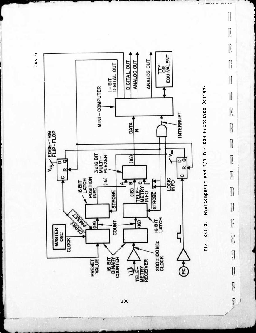
i^^
0>
CVJ
c en
•r—
LO
QJ
Q
0) Q-
o s.
o Q:
s. o
(U ••J 3 Q. E O O
n i
i—i x X
C7>
330
i I
n
i
i
ii
n
j j AIMII m mmmm

I I I I I I I I
SECTION XXI
TABLE I
Minicomputer Specifications
Word Length 16 bits
Instruction Types Required Maximum Time per Instruction
Add, Subtract, logica il and, logical or 2. 5 ^sec
Shift one bit right or left 2. 5 fisec
Memory fetch and store 2. 5 (isec
Jump and conditional jump 5 fisec
Multiply 12 lisec
Divide 15 jisec
Access IO channels 5 (isec
Storage Required
8K of 16-bit words
I/O Ports
2-16 bit input ports | preferable but not necessary
1-4 bit input ports j 1-16 bit input is minimum requirement
2-16 bit output ports
1 interrupt input
1 teletype interface
Software
Cross-assembler (preferably compiler) for IBM 370/165 — paper tape output
Core-resident paper- ■ tape loader fprefe rably ROM backup)
Peripherals
1 Teletype ASR such as ASR 33
T872
1 331
A-^

I I I I 1 1
I
SECTION XXII
PHASE II DIGITAL SYSTEM BENEFITS
A digital data reduction subsystem is required to obtain the
accuracy and resolution necessary to measure gradients of ±4500 EU
to an accuracy of 1 EU. Although it would be possible to build the
digital data reduction subsystem using discrete components, a minicom-
puter is i more cost-effective solution. Once a minicomputer was
made a part of the prototype design, it became apparent that it would
provide significant benefits during Phase II of this development pro-
gram. These benefits are discussed in the following paragraphs.
A. COMPUTATIONAL REQUIREMENTS COORDINATION
Sub-Line Item 0002AC of the Statement of Work for this develop-
ment program requires the following: "Determine op .rational and
computational procedures to obtain average gradients for 10-second
intervals in terms of EU such that the procedure will not contribute
more than 0. 1 EU error." This has been accomplished already.
The procedure required to obtain any gravity gradient tensor component
from individual gradiometer outputs was shown in the original proposal.
These gradiometer outputs have been established in digital form and
can be combined easily by the digital computer.
B. DIGITAL ROTOR SPEED CONTROL
It was stated in Section XVI, Rotor Speed Control Subsystem,
that the prototype design was based on an analog speed control servo
loop using a tachometer as the basic velocity feedback. This, although
satisfactory, requires extreme care in amplifying the tachometer
signal.
Preceding page blank 333
■—- ^MÜ tammmmimmm

:«
SECTION XXII
It was shown in Section XXI, Digital Data Reduction Subpvstem,
that an output pulse would be generated each 1/8 revolution (~140 per
sec) of the sensor rotor with an instantaneous position uncertainty of
no more than 2. 2 x 10" rad, 1 sigma. Since the average speed of
the rotor is known to seven significant figures, the number of cycles
of the 10 MHz reference that should occur during 1/8 revolution of the
rotor can be calculated and prestored in a computer register. A
counter can count the number of 10 MHz cycles that actually occur
during each 1/8 revolution as determined by the above mentioned posi-
tion pulses. The difference between these two counts is the position
error accumulated during 1/140 second, or an error rate signal. The
average of this error rate signal is excellent, but each output is noisy
due to discrete quantization levels.
If the demands on the rotor speed control servo were not so
severe, the noise in the above mentioned error rate signal could be
ignored and a straightforward digital servo designed. However,
presently available analysis methods are not adequate to predict the
performance to the level required in this application.
It is estimated by some digital servo experts that satisfactory
performance can be obtained by experimentation after the sensor is
built and operating. However, this is not sufficiently certain to be
used as a prototype design. Therefore, the prototype design will
include a digital servo and an analog servj. The analog will be used
in initial tests and then the digital servo will be mechanized. It is
expected that the digitil rotor speed control will be used in the final
tests.
C. ACTIVE COMPENSATION OF THE RGG
Because a digital computer is now a part of the prototype
design, active compensation concepts now are attractive and feasible.
Active compensation, as defined by Dr. Dan DeBra of Stanford
University, uses a computer model of the RGG sensor to correlate
I
I
I
1 I
I
II
i(
l( I
334 I

I !
I 1 I 1 0 i I I I t 0 t I I I I
SECTION XXII
casual inputs with sensor outputs and correct the sensor or the data
output on a real-time basis for changes in the sensor. For example,
there will be a continuous variation in the acceleration along the
sensor X axis. Ideally, the'sensor will not respond to this variation;
however, if the sensor output contains a signal that is exactly corre-
lated with this casual acceleration input, output could be caused by
imperfect arm anisoelastic compensation. The computer would be
instructed to change the compensation calculations until the effect
disappeared. Another example of active compensation that may be used is ai
follows: The sensor test signal described in Section XVII would be
turned on and off at 1 sec intervals. If the sensor id operating at
exactly the proper frequency and therefore the proper output signal
phase, this test signal will all appear in one channel and can be sub-
tracted out of the data. However, if some of the test signal appears
in the other channel, the computer will know that the reference spin
frequency is incorrect and also how it should be changed to correct
the phase angle. The computer can be instructed to make this fre-
quency change automatically. The active compensation concept will be studied during
Phase U.
335
■«•»■»««■•■••""^
MM ^M^i

I I I I r r
i i
SECTION XXIII
RGG CALIBRATION TECHNIQUES
The RGG is a new inertial sensor, and standardized test,
calibration, and evaluation procedures have not been established.
Some of these procedures have been developed by Hughes during the
earlier experimental development work on the RGG. Standardized
procedures have been developed for gyroscopes and accelerometers
and r-'any of these concepts are believed to be applicable to the RGG,
The following paragraphs illustrate some procedures that Hughes
expects to utilize during test and calibration of the RGG.
A. BIAS ADJUSTMENT
1
The sensor will be mounted on a level, vibration-free base
and allowed to stabilize, first with the spin axis vertical. The sensor
case will then be rotated in 3*. precisely indexed steps about the spin
axis. The sensor output, averaged over a period of 1 min, will be
recorded at each index position. Since sensor biases are case fixed,
they will not change as the sensor is indexed around. The local gravity
gradient, local earth's magnetic field, local masses, and initial spin axis
tilt (if any) will remain constant and earth-fixed as the senior is rotated.
A 32 point Fourier analysis will allow determination of the sensor bias
coefficients in terms of direction and magnitude of the local gravity gradient,
Once the sensor bias has been determined, the operating tem-
perature will be changed slightly and the sensor retested. The change
in temperature will aid in determining the following five character-
istics: temperature sensitivity of the sensor undamped natural fre-
quency, temperature phase shift sensitivity, spin bearing drag tempera-
ture coefficient, and the phase and scale factor sensitivity of the signal
readout subsystem.
Preceding page blank 337
^^_

SECTION XXIII
The sensor will be turned to place the spin axis in a horizontal
plane and the above procedure repeated. In addition to the parameters
previously mentioned, the anisoelastic torques of the sensor arms are
added to the fixed torques.
Fl
B. SCALE FACTOR CALIBRATION
Accurate calibration of the absolute scale factor of the RGG is
accomplished best by introducing accurately known angular rates at
right angles to the sensor spin axis. These rates can be introduced
best by mounting the sensor on a precision rate table or on a stable
platform that is commanded to precess at a specific rate in inertial
space. In either case, a completed operating sensor is required.
The sensor can be calibrated to an accuracy of about 2. 5 to 5%
during assembly by adding accurate amounts of arm mass unbalance on
arm inertia unbalance. The sensor is then vibrated as appropriate to
excite the desired unbalance mode. These methods are simple and
convenient, but the overall accuracy is not adequate for the completed
RGG. There are a number of other methods of obtaining approximate
RGG calibrations, but none so far discovered can approach the accuracy
of the two just described.
C. ARM MASS AND INERTIA BALANCING
Three unbalance parameters are of importance in precision
balancing the sensor arm pair. These are: (1) arm sum mass unbal-
ance, (2) arm differential mass unbalance, and (3) arm sum mode
mismatch. The first, arm sum mass unbalance, is defined as the sum of
the individual arm unbalance vectors. The individual unbalance
vector is defined as the distance between the individual arm center of
338
i
i B a
n 8 1
1 U

SECTION XXIII
mass and the elastic (torsional) axis of its support pivots. Thus the
sum of these two unbalance vectors must be initially adjusted to a
specified minimum value (8 x 10'J gm-cm).
Arm differential mass unbalance is defined as the difference
between the individual arm mass unbalance vectors and also must be
adjusted to a specified minimum value. Because of the sensor's con-
siderably larger sensitivity resulting from differential mass unbalance,
it must be adjusted to very close tolerances, and this is accomplished
in two steps. First, it is adjusted via mechanical balance screw
adjustments to within the specified limit of ±8 x 10" gm-cm. Then
fine balancing is accomplished using the mercury balance tubes dis-
cussed in Section XVII.
The third unbalance parameter, ar-^> sjum-mode mismatch, is
due to a mismatch of the ratio of support pivot spring rate to arm
mass moment of inertia between the two arn::. This error may be
reduced by adjusting either the support pivot spring rates or the
moment of inertia. Spring rate matching is difficult because it would
require trimming material from the support pivots that is relatively
inaccessible. Moment of inertia balancing achieves the desired result
and is considerably less difficult. Mechanical balance adjustment
screws can be used to adjust the sum-mode mismatch to the required
level of AI/I = 1C"7.
The three unbalance parameters result in RGG sensor error
sensitivities to different types of vibrational inputs. The arm sum
mass unbalance gives rise to a sensor error proportional to angular
vibration normal to the sensor's spin axis. Sensor arm differential
mass unbalance produces sensor errors proportional to the transla-
tional vibration normal to the sensor's spin axis. Sum mode mismatch
results in sensor errors proportional to angular vibration about the
spin axis. Thus, by exposing the sensor to the excitation sources,
one at a time, the sensor output signal can be used as a means of
sensing the amount of unbalance present. Thus, adjustments of the
339
Ml
1! SECTION xxm
balance screws can be made to null the sensor output for each of these
three types of excitation.
Hughes has developed experimental techniques that can produce
these separate excitations at the required levels. These techniques
are discussed in detail in the HRL Technical Proposal (see Section V-D),
pp 143-147. For fine adjustment of the differential mass unbalance, the
same test techniques will apply. In this case, the entire rotating
sensor and its temperature-controlled housing will be exposed to a
pure translational vibration, the output signal monitored, and the mer-
cury balance adjustment device driven until the sensor signal is
nulled.
D. ROTOR MASS BALANCING
Hughes also has developed laboratory techniques for achieving
accurate static and dynamic mass balance of the sensor rotor. The
sensor stator is suspended on very low mass, compliant ppring sup-
ports. Static and dynamic mass unbalance is sensed by use of sensi-
tive geophone pickups (velocity meters), one oriented normal to the
spin axis direction and one displaced from and parallel with the spin
axis. The phase of the unbalance is determined by use of a strobe
light, triggered at the ^ero crossing of the geophone signal output.
Static mass unbalance has been adjusted to a 1-microinch accuracy
using this procedure.
340
fl
i
i
1
i
1 i
1
1
1 1 1 B 1 I B
^rik mm

'
I I I \
\
SECTION XXIV
LABORATORY EXPERIMENTS
A. VIBRATION SENSITIVITY MEASUREMENTS
Testing on the prior test model of the RGG indicated a sensitivity
to acceleration applied along the sensor spin axis. Recent quantitative
testing indicated the magnitude of this effect was approximately 2x10
EU/g (under an applied 0. 001 g drive input acceleration).
Two mechanisms each of which could have caused such sensi-
tivity are analyzed in the following discussion. The first mechanism
is simple tension and compression in the central transducer structure,
generated by a mismatch in the tensile spring properties of the arm
supports. The second mechanism is moment loading of the transducer
ends due to congruent mass unbalance on each of the arms. Each of
these mechanisms is capable of generating greater than 10 EU/g
under quite reasonable assumptions of the magnitude of the existing
errors.
B. ANALYSIS OF GRADIENT STRAIN LEVEL
To establish the magnitude of these effects we should first
calculate the equivalent gradient-strain level scale factor. The
maximum bending stress in the quadrilever pivot for a unit torsional
input has been calculated by D. W. Rouse to be
CTB 6Erc (1)
and the associated strain(og/ej/g (maximum)
€B 6xc
341
mm

SECTION XXIV
however, a transducer which covers 1/4 in. of the 1-in. long leaf
senses the average strain or 3/4 of the maximum
4i2 /•B\ _ 3 6TC or ^_ = J" l-T-javg - 4 p 'B
T^
where
i = 1 in.
r = 0.40625 in.
c = 0.0205 in.
JL = Z6.683 in.
rac (2)
The gradient sensitivity (angular deflection) of the sensor
is giv^n by
Tr o = J- r ^T
(3)
where T gradient torque = ^ Ja req/2 and
KT s T + K
where
K a end pivot spring rate
K = c o entral transducer spring rate
i
1
i i
1
i
1
1 I
1 11
1 i
n 342 r
*m*

1 SECTION XXIV
r i
Therefore
or r _ eq
er : . ^a " K + e o
^a or e K + 2K e o
K + 2K n J
(4)
(5)
I I
'
We can now multiply (5) by (2) to obtain the gradient-strain level scale
factor (EU per in./in.). We obtain
B
K , 2K e + o 1 J
41 18rc
x 10
Sensor parameters were measured as follows:
g K = 4.5x10 dyne cm/rad
g K - 4.86 x 10 dyne cm/rad
0.7
J = 28,600 gm cm a
i =
r r
1 in.
0.5 --TT"1*
= 0'40675 in. = 1.032 cm
c = 0.0205 in. = 0.0521 cm
343
(6)
— ^^^r

»v
SECTION XXIV
Inserting these values into (6) we can evaluate the scale factor:
-sSa .= 1.895 x 10¹⁵ j-SS- «. in. /m.
(7)
C. ANALYSIS OF TRANSDUCER MISMATCH
The effect of dimensional tolerance of the transducer itself
depends on the type of strain h^ing sensed. For pure tension and
compression in the leaf, the voltage equation is
V T TW §3! = «rg
31
so a 10% variation on the transducer thickness will produce a 10% vari-
ation on the voltage output. In addition, of course, the output voltage
varies with changes in transducer output impedance, but these changes
produce only a 1% variation in voltage per the rms dimensional
variation of the transducer, and can be neglected.
For bending strain, the transducer no longer senses a constant
strain level, but an average strain under its area. Therefore the
length and position of the transducer are both important. A 10% length
variation (0.025 in 1/4 in.) will cause a 5% variation on the average
strain sensed, whereas a 10% change in position will cause a 10%
change in average strain. If we rms these with the 10% thickness
variation we get a ±1 5% variation on the output voltage.
I
"I
!
I
i
1
1
344
I
0
i
i
n
mam

^M
SECTION XXIV
D. TENSION-COMPRESSION DUE TO AXIAL ACCELERATION
Ideally the RGG would be insensitive to axial acceleration
because of its axially symmetric construction. However, the two
outer supporting plates do not have the same thickness and this thick.
ness assymetry causes strain to appear on the central flexure under
axial acceleration. The sensor model for this effect is shown in Fig. XXIV-1.
M
107S-47
^—I
—I
Fig. XXIV-1. Sensor Model Axial Acceleration Effect,
Htre
K = K,= end pivot axial stiffness 1 Cm
K.= quadrilever pivot stiffness
K K = diaphragm stiffnesses of end mounting plate 41 5 (K4 ^ Kg)
for the end pivots the axial stiffness is given by
Kl - K2 " i (8)
345
*mtk

SECTION XXIV
where
A = ffr2 = ff(0.030)2
i = O.OiO
E = 30 y 10
K1 = K2 2.12 x 10⁶-^ in.
For the central flexure
K. 4AE
where
A = leaf cross section =(0.041)(y^)
i = 1 in.
K3 = 9.23 x 10⁵^
K. and Kc are diaphragm spring constants of the form 4 5
K = 27r E m2 t3
Ip-Vo)- V; I0« T 'o
where
m = 1
alum
a = radius of plate = 3 in.
346
(9)
(10)
(ID
(12)
I
1
1
i
!
1 "1
1 1 0 I D 0 B
/
*^*^^mf^mam u

■■
SECTION XXIV
t = thickness of plate tj =0.5, t^ = 0.75
E = 10 x 106
r = Effective radius = yiMv)* + (t)2 - 0.675t (13)
where r = radius of applied load =0.5 in.
when t = 0. 75
r = 0.475
K. = 2.363 x 10' 4
(14)
and when t = 0. 5
r0 = 0.469
K5 = 0.699 x 10 (15)
347
^^^

SECTION XXIV
Combining these diaphragm springs with the end pivot spring rates, we
obtain
TrB- K-Z +ir4
KB 1.117 x 10° lb/in. (16)
(17) 1 = * + *_ K = 0.526 x 10⁶ lb/in. KT Kl K5 T
We can now find the strain in „he center pivot by putting the system
under constant acceleration and writing force equations from free
body analysis
+ K3(x1 - x2) - KT x2 = ma 1 (18)
KTX2 K 3(x1 -x2) - KgXj = ma (19)
m
K3(x1 - x2)
K3(x1 - x2)
1*2
m
KBX1
2K3(x1 - x2) - KT x2 + KB Xj = 0
2K3 Xj + KB xj = 2K3 x2 + KT x2
Xj 2K3 + KT
*- = 2K3 ? KB
It is simpler now to solve for this ratio and then complete
the solution
2(0.924) + 1.117 2(0.924) + 0.526 1.249
or x. = 1.249 x2
348
I
■I
1
1
1
0
II 1
Ü
B 1
"1
0
n n n /
- ^MHM ^^^^mtmmmmmm

^
SECTION XXIV
Therefore
K3(1.249 X-, - x2) - KT x2 = -ma
(0.249 K3 - KT) x = -ma = -W (for lg acceleration)
-W x2 0.249 K3 - KT
2.054 x 10" in. (20)
and
K1 = 2.565 x 10" in.
Xj - x2 = 0.511 x 10"6 in.
(21)
(22)
which is the strain in the quadrilever.
If we multiply this strain by the gradient strain factor
determined earlier, we obtain an equivalent gradient signal
15, S T = (0.511 x 10-b) (1.895 x 101D) = 9.683 x 10° EU/g (23) eq
If we assume that 10% of that signal is not rejected by transducer
matching (see Section XXIV-B above) this would leave an axial tension-
compression sensitivity of
r = 0.968 x 10⁸ £2 eq g
(24)
349
^g^

SECTION XXIV
E. ANALYSTS OF CONGRUENT ARM MASS UNBALANCE EFFEC'.S
The method of balancing which was used to adjust the arm
balance of this model of the RGG was designed to eliminate only the dif-
ferential unbalance between the two arms. After the complete balancing
operation there could still be a large common unbalance where each
arm C of M was offset from the pivot support. This unbalance, when
excited by axial vibration could excite a parallelogram type bending in
the center flexure and the resultant S shaped bending in the leaves of
the flexure would generate gradient error signals in the transducer.
Analysis;
The model chosen for this analysis is to replace the end
pivots with pin supports (the pivots are much stronger in tension
and compression than in bending) (see below). Each arm has an unbal-
ance of the same magnitude and sense away from the pivot support line.
207S-4S
A tin OJT
350
I
!
!
I
i
i
I
1
"I
n i
si ii
n /
■ *tm *m*

I ]
I ]■
SECTION XXIV
Each beam"of the center flexure could be analyzed as though it were
pin supported with moments of
10T5-«« M M
similar sense about each pin. The deflection of the beam would be
«079-49
MoQr7
with a moment diagram
2079-46
+ M,
The angle 9 is given by
i i I
M(x)dx El
Mo(l) nrr
Moi
351
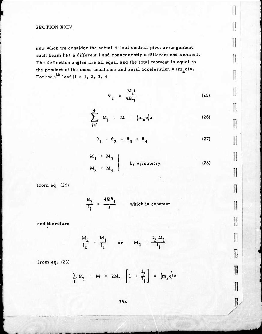
SECTION XXIV
now when we consider the actual 4-leaf central pivot arrangement
each beam has a different I and consequently a different end moment.
The deflection angles are all equal and the total moment is equal to
the product of the mass unbalance and axial acceleration = (m e)a.
For'he i leaf (i = 1, 2, 3, 4)
M.I i
4EI.
2^ M. = M = (mae)i i^l
ei = 92 ' = 93 = 94
M1 = M3
by symmetry uz = M
4
from eq. (25)
M. 4Ee. i
I. i
i
i which is constant
and therefore
M2 Ml l2 Ml __ = __ or M2 = —I
from eq. (26)
J M = M = 2MJ 1 ^
= (mae)
(25)
(26)
(27)
(28)
352
I
I :
"i
1
D i
1 n E 1 "!
"i i
II D n
/
ii i ■ ■■

I
I I I 1 I 1 I r
i i [ i i i i i
SECTION XXIV
therefore
M, (mae)
"V. M. Ke)
1+i The root strain in the leaves is given by
M. c. i i
"El-
and since the transducers ar-- placed in such a way as to read the
strain in the thinner ben<Ung section leaf only, this is the strain which
is seen in the output
(mae) a c
1 + 1 J
El,
bhJ hbJ
where
h = 0.041 in.
b = -^ in.
c = 0.020 in.
m = 1.87 lb a
1.077 x 10"6 in.4
2.252 x 10"5 in.4
353
- ~ - — '- ^m*t

SECTION XXIV
We assume a mass unbalance eccentricity of 0. 01 in. and calculate the
per g strain
_L B 2.6416 x 10" in./in./g
)r the average strain under the transducer
!•>
"7
= 1.981 x 10" in./in./|
when we multiply by the strain sensitivity calculated previously
15 (1.895 x 10 EU/in. /in.)
we obtain a signal level of
3.754 x 10⁸ EU/g
The transducer matching to within 15% discussed in Section B leaves
an uncompensated signal of
0.5631 x 10⁸ EU/g
The rm? of this effect with the tension compression effect previously
calculated (Section XXIV-D)
1.120 x 10⁸ EU/g
certainly close to the experimental results.
354
1 1
1 1 1 1 1 1 1 1
1
tl
■I
0 11
IU / s
^M-^fl^il MBMi

XIV-1.
XIV-Z.
XIV-3.
XIV-4.
XIV-5.
REFERENCES
W. P. Mason, Editor, Physical Acoustics, Part A-Methods and Devices, 1964, Academic Press.
W. P. Mason, Electromechanical Transducers and Wave Filters, 2nd Ed. , 1948, D. Van Nostrand and Co.
H. W. Katz, Editor, Solid State Magnetic and Dielectric Devices, 1959, John Wiley & Sons, Inc.
E. G. Thurston, Theoretical Sensitivity of Three Types of Rectangular Bimorph Transducers, Journal Acoustical Society of America, Vol. 25, No. 5, (Sept 1953), pages 870-872.
H, Jaffe \nd D. A. Berlincourt, Piezoelectric Transducer Materials, Proceedings of the IEEE, Vol 53, No. 10 (Oct 1965), pages 1372-1386.
n
355
■ - -■
aaMfl_^^ *mmm

APPENDIX A
SENSOR ARM ANISOELASTIC DEFLECTION ANALYSIS
This appendix presents the assumptions and results of an arm
structure deflection analysis for the baseline arm configuration. These
results have been used to determine an optimum set of arm dimensions
to achieve anisoelasticity as well as high structural stiffness.
1. Arm ConfiRuration
The sensor arm configuration analyzed herein is shown in
Fig. A-l. It consists of two parallel plates whose ends are fastened
together via heavyweight end masses. Fastening of each plate to the
end masses is accomplished using multiple screws through each plate
end into tapped holes in the heavyweight material. The plates have cut-
outs as shown to reduce the longitudinal stiffness in order to make it
equal to the lateral bending stiffness.
2. Assumptions
In this analysis, the compliance of only the center of mass of
each arm end mass is computed. The anisoelastic error coefficient is
a function of the distributed mass-deflection characteristic of the total
arm structure as well as the end masses. The structure mass-
deflection has been ignored in the analysis. This is justified since the
mass of the structure is only I/6th that of the end masses and only a
small portion of the structure mass undergoes a significant proportion
of the end mass deflections. This will be taken into account during the
assembly and trimming operation mentioned in the text of Section XIII.
Any internal deflections of the end masses have been ignored
because of the relatively larger elastic moduli.
i
357
Preceding page blank

t07B-t7
0.979 in.
0.725 in-
0.350 in.
V rHv^fm
r 0.675 in.
I I v
TZT
L ' i i
tt .._£ JL--
I.l8lin. 1.305 in. M
■ 1.443 in. 2.376 in-
O.lin.DIA.(TYP)
2.00 in,
Fig. A-l. RGG Isoelastic Arm Design.
1
358
1 1 1 1 1 1 1 1 1 1 1 1
ii
II
- - MBMMMI Ml

I I I I ]
1 I I 1 \
I
APPENDIX A
3. Idealized Structure
The baseline arm configuration depicted in Fig. A-I has been
simplified to allow straightforward analysis of each component member
of the structure. The idealized arm structure considered in this anal-
ysis is illustrated in Fig. A-2. The heavy dotted lines represent the
elastic axis location for the members considered to deflect elastically.
The shaded portions were considered infinitely rigid. The dimension
symbols represent the length of each of the elastic members. In the
analysis, the width of each member is denoted by w., i being chosen
consistent with the member's length dimension symbol. The thickness
of the arm plate is denoted by t. Dimension d denotes the spanwise
location of the center of mass of the heavyweight end mass. An x, y
coordinate frame is shown for reference. All interconnections between
the elastic and the infinitely rigid members are assumed to be "fixed"
or "cantilevered" joints. In computing deflections of component mem-
bers of the idealized arm structure, stiffness contributions of fillets
have been ignored; however, flexure as well as vertical shear effects
are included in all bending computations. For member e, its width has been assumed to vary linearly with
its span in all deflection calculations. Arm anisoelastic error torques are induced by static or vibratory
accelerations of the arm support pivots. In deriving these compliance
equations, the induced inertia loads of the end masses have been
replaced by static loads and similarly, the support pivot acceleration
induced loads replaced by static reaction forces. No account has been
made for dynamic structural deflections in replacing the "acceleration-
induced" loads with "static" loads. For analytical convenience, all
compliances were computed considering only half of one arm plate. The
boundary conditions assumed in deriving each compliance equation are
illustrated in Fig. A-3. The equations for arm end mass deflection have been derived
based upon the above stated assumptions. The compliances in each of
I 359
^mtmt

Fig. A-2. Idealized Arm Structure.
360
tors-ta
»X
i
!
1
— I
1 1 1 1 1
1
B B B I B
J ~m^^^m*mmmä

^
i
2079-29
(a) LONGITUDINAL
i i a -I (b) LATFTiAL BENDING
s
(c) AXIAL BENDING
NOTE: VERTICAL GUIDES PREVENT ROTATION OF THE END MASS ABOUT ITS LATERAL ly) AXIS.
Pia A-3. Assumed Boundary Conditions and Loads for Compliance Evaluation.
T ■-■ :-mm
361
riMM»

i APPENDIX A
the three principal axis directions are defined by the ratio of the end
mass deflection, 6., to the applied load, P.: 1
C = —. C = -i. c = — x P y P z P x 7 y z
The resulting compliance equations are:
Cx = Et z b
2w3 + 2w£ a
a£n(l - pe)
w p eore (A-I)
C = ^T 1
Et 2(a + c/2)' -\^ j bE
?,GWn 2w 2b-
w.
/ 3
w eo
(A-2)
where
i, b, c, d, e, i
w. i
w eo w el
length of members (see Fig. A-2)
width of members (see Fig. A-2)
width of member e at root, or center of arm
width of member e at tip = c
taper ratio of member e
w eo w
eo
E
G
Young's modulus of elasticity
shear modulus of elasticity
K, ^ + ^)Mi - Pe) + Pe(1 - Pe) + lPe
PIU - Pe)
An explicit equation for the axial bending compliance is too unwieldy,
hence intermediate parametric functions and a final equation in terms of
these parametric functions is presented.
362
1 1 I 1 1 ]
B "i
"I
1
"i
I ^^»ft

I I I \
]
1 1 I I I I I I 1 1 I I 1
APPENDIX A
Define;
K p A V 6b 12EI.
3EL 1 +
b2AbG
K M A b 6b 2EL
K5. * £ Ob " 8EI,
K M A b Bb EL
K A b
ob GK.
K P 4 a' 6a 12EI
1 + 3EI a
a2A G a
K M 6a " 2EI
K P 4 _a_ Ga 8EI
K M A a Ga El
K 4 _ä_ aa GK,
K P 4 6e 2EI6P
e
1 + EI^P
e
e A G e
K M A e 6e EI6M
e
K P 4 S Ge 2EIeP
e
K M £ e Ge EI6M
e
where in the above, the following definitions apply
.th I. = section inertia of i member
K K = Torsional section inertia parameter given by a' b
363
^^^■Mtf^^l
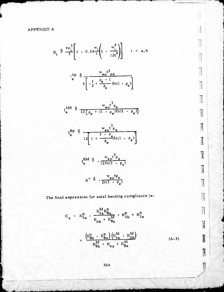
■" ■■ "^ •
APPENDIX A
K. - 3 w. / w.
i - O.M-MI - —4 w4\-
m4) = a, b
T6p A w t3
eo pe
'
I 6M A
2+ V-£n(1- pe)
w t P- eo re
5 12[pe + (1 - Pe)«n(l - pe)j
rep A
12
w * P^ eo Ke 1 - o
1 + EZwT^]
i
3 GM A weo pe
TziMl - PJ
w tp « A eo re
£n(l - Pe)
The final expression for axial bending compliance is:
oa
KM
KP
,,M ob öe
K-«L)(K fee " K6bj
KQh + Kaa + Kee
364
(A-3)
!
"
11 ■;
i
i
1 \
0 1 I I
H
•«■^Ma rinMü
APPENDIX ß
ESTIMATION OF UPPER BOUND OF STABLE PLATFORM ANGULAR RATE
I I
The second order gradient of the specific force field at a point
in a gravity field (as viewed by an observer in rotating frame of refer-
ence) is a linear combination of the second order gradients of the grav-
ity and rotational fields. All so-called gravity gradiometers are
actually specific force gradiometers; and because of this, the measure-
ments of such instruments are contaminated by the inertial angular
velocity of their measurement frames of reference. To obtain the sec-
ond order gravity gradient tensor elements from a system of such
instruments, it is necessary to correct for the rotational field effects
on the measurements of these instruments. The differences between
the actual rotational field gradients and the quantities employed for
compensation are defined as the "rotational field measurement errors. "
In the present application, it is desired to estimate the rotational
field errors which would occur if the gradiometers were directly
mounted to the platform stable element. In this case, the inertial
angular velocity of the stable element is the angular velocity of the
measurement reference frame. This inertial angular velocity may be
considered to be inade up of the sum of two components, a deterministic
portion and a random portion. It is intended that the gravity gradien,.
measurements are tobe compensated for the gradient cf the deterministic
portior of the rotational field and that the remaining portion of the
rotational field gradient be classed as a rotational field error.
The deterministic portion of the platform stable element inertial
angular rate woula be, for example, the carrying vehicle's transport
rate plus the earth's rate for a north referenced, locally level platform
mechanization. Measurements of these quantities would be the gyro
precession command signals obtained from the platform's management
computer. The random portion of the platform stable element inertial
365

APPENDIX B II angular velocity will be mad*» up of various disturbances including gyro
drift rate, gyro signal noise, and oscillatory angular rates induced by
mechanical torque disturbances such as gimbal bearing friction, accel-
eration induced platform mass unbalance toroues, etc.
Rigorous calculation of the rotational field errors in the mea-
sured gravity gradient tensor elemsnts requires a complete knowledge
of the angular rate spectra of the stable element, i.e. , the three
co-spectra and the three cross-spectra. Althcugh rigorous calculation
of the rotational field errors is not possible in the absence of these data,
it is possible to estimate the upper bounds on these errors from the
limiting values of stable platform disturbing functions.
One of the predominant sources of platform disturbance is a
result of interactions of angular rates of the platform's base with the
coulomb-type friction torque associated with the platform gimbal bear-
ings, slip rings, residual torque motor torques, etc. , and the plat-
form's stabilization servo. The manner in which this disturbance
propagates into platform stable element angular velocity depends on its
spectrum and on the stabilization servo's response to torque distur-
bance. Precise analysis to generate the required angular velocity
motion spectra is very difficult and would require development of a
complex and costly computer simulation model and accurate knowledge
of the angular rate motion co-spectra and cross-spectra of the stable
platform's base.
In the absence of this data and the computer simulation model,
an upper bound of the platform angular rate variance may be determined
on the basis of the following heuristic argument. First, an upper bound
can be placed on the variance of the normalized disturbance torque.
For example, consider the normalized disturbance torque to be a zero-
mx-'an, random variable, x, with probability density, p (x). The var-
iance, (r , is just the second moment of the density function as in (I).
1
/CO
x
00
■px(x)dx (D
W
366
I
"1
1
1
i
fl fl 11 11 H
%
tfMMM jam

I I I I
APPENDIX B
When the random variable is bounded to a maximum value, x , then 2. max'
ita variance is bounded to x . The limit is reached when the proba- max r
bility density functions, p (x), consist of a pair of impulses located at
±x as in (2). max
r Px(x) = \/z\bU ) + 6(-x )! L max max J limit
(2)
for any other probability density function bounded by ±x , the variance 2 rricLx
will be less than x as stated in (3). max
2 2 or < x x max (3)
1 i
r
This bounds the variance of the torque disturbance by its maximum
value. Next consider the platform angular rate response to normalized
disturbance torques as in (4).
Vs) V8)(ir) (4)
From (4) the angular rate power spectrum is stated in terms of the
torque disturbance spectrum, S,(f) as (5).
\
I I I I n
s (f) H {j2TTf) p J •sd(f)
The rate variance is obtained by integration of (5) as in (6).
U) JL Sw(f)df=riHp(j2TTf) 'Sd(f)df
367
(5)
(6)
■ mmm

APPENDIX B 1 An upper bound on the rate variance of (6) may be determined by
forcing the disturbance torque spectrum to have all of its power at a
frequency where the platform response, H?(s), is a maximum. Thus
the rate variance is bounded as in (7).
max p max (7)
max
An estimate of the peak disturbance torque response is given by (8)
where u is the platform servo bandwidth and 2, is its damping b
coefficient.
Hp(s) max N/24W>
(8)
Using eqs. (7) and (8), the estimated upper bound of rate variance is
given by (9).
er2 S —i—cr I2
oj _ „ 2 2 dl 2£, w, | max (9)
where (r2l is taken to be the coulomb friction torque level normal-
ized by plIRform inertia. Thus, the standard deviation of this bounded
ingular rate estimate for coulomb-type friction disturbance is
N/Z& wbJ
(10)
A method of computing an upper bound for the stanc'ard deviation
of platform angular rate has been established. This upper bound was
established in the absence of any knowledge of the form of the distur-
bance spectra using a probabilistic argument. This approach did not
368
D D B
I 1 n

"" 'P
APPENDIX B
lead to an estimate of the form of the angular rate spectra necessary
for rigorous calculation of the rotational field errors of the gravity
gradient tensor elements; however, by a similar probabilistic argument
in Section IX, Error Analysis, using the angular rate bound developed
here, an upper bound of the gravity gradient component rotational field
errors is demonstrated.
1 I
369
- - --* ^M* mmm

■■ ■P " • ' 'W
APPENDIX C
SPIN MOTOR SPECIFICATION
J7J I - ^^^üflBMmM
PROCUREMENT SPECIFICATION
for
SPIN MOTOR FOR HUGHES
PROTOTYPE ROT/ TING GRAVITY GRADIOMETER
Date: September 5, 1972
No. RGG 1 Revision B October 4, 1972
Approved by:
D.W. Rouse
Hughes Research Laboratories 3011 Malibu Canyon Road Malibu, California 90265
Preceding pagesNank
Page 1 of 14 373
— I I1IÜ

^r
i
TABLE OF CONTENTS
1. 0 Scope
2. 0 Applicable Documents
3. 0 Requirements
3.1 Conflicting Requirements 3.2 Materials, Parts and Processes 3. 3 Gravity Gradiometer Description
3. 3. 1 Sensor Physical Parameters 3.4 Spin Motor Performance Requirements
3. 4. 1 Second Harmonic Torque Ripple 3.4. 1. 1 Deterministic Torque Oscillation 3. 4. 1. 2 Random Torque Variations
3. 4. 2 Torque Oacillations at Other Frequencies 3. 4. 3 Spin Mocor Full Load Speed 3. 4. 4 Spin Motor Torque 3. 4. 5 Torque Speed Curves 3. 4. 6 Rotor Vibration 3. 4. 7 Input Power 3. 4. 8 Spin-Axis Alignment Reference 3. 4. 9 Electrical Insulation
3. 5 Environmental Conditions 3. 5. 1 Operating Performance Condition 3. 5. 2 Operating Standby Condition 3. 5. 3 Non-Operating Condition
3. 6 Leliability Objectives
4.0 Quality Assurance Provisions
Figure 3. 3 Rotating Gravity Gradiometer Baseline Configuration
Figure 3. 5. 3 Acceleration Spectra
Table 3. 5 Environmental Conditions
Page 2 of 14 374
I
n i i n
i D fl
1
li
H
fl
mm *mt

REVISION B CHANGES
P*i*
6
8&9
10
12
Para.
1. 0
3.4
The gradiometer de iign has been changed to use two identical spin motors in parallel. This specification is for a single motor. Thus many of the limits, such as full load torque, torque ripple allowed, etc. , have been halved in the body of the specification. However, Hughes has also elected to use oil lubricated spin bearings - the total sensor running torque has not changed - and the starting (break-away) torque require- ment has approximately doubled.
"harmonics" has been clarified to show that it is torque harmonics that are of interest to Hughes.
3.4.1.1 These paragraphs changed to reflect the requirements 5. 4. I. t on a per motor basis. 3.4. ^ 3.4.4, a,b, c 3. 4. 6,a,b
3.4. 7 The locked rotor power is not especially important. Nor are torque variations, waveform distortion or heating during sensor breakaway and run up. However, Hughes is interested in the highest practical efficiency after the sensor has stabilized at running speed. Motor losses will heat the sensor and thus make it more difficult to maintain extremely accurate temperature control of the sensor which is required. *
Fig. 3. i This figure has been changed to show the use of two small oil lubricated bearings. Both the inner and outer stator radial thickness can be increased as shown in the figure if this is desirable. It is desired that the outer diameter of the outer stator ring be limited to 3. 0 inches unless this leads to a very unwieldy motor design. The axial length of the motor may be increased if required but again the shortest practical length is desired.
* Pole changing for break-away torque and initial runup may be
considered if switching is not too complicated.
I
L
Page 3 of 14 375
^M

PROCUREMENT SPECIFICATION FOR
SPIN MOTOR FOR
PROTOTYPE ROTATING GRAVITY GRADIOMETER
I fl
1. 0 SCOPE
This specification covers the requirements for a spin-axis
drive motor for a prototype moving-base rotating gravity
gradiometer, which may be herein referred to as the "sensor. '
The spin motor will be used as a part of a servo control loop
to drive the sensor rotor at a speed of exactlv 1050 RPM. Two identical spin motorc, connected in paraael, will be
used on each sensor as shown in Fig. 3. i. This specifica-
tion gives the requirements for each individual motor. The
sensor constitutes the basic sensing element in a system
designed to precisely measure gradients of the gravitational
field from a moving vehicle. The requirements and environ-
mental conditions associated with the sensor necessitate that
the spin motor perform its function with great precision as
well as being rugged, reliable and reproducible.
2. 0 APPLICABLE DOCUMENTS
The following documents in their latest issue at contract date
form a part of this specification to the extent specified herein.
Specifications —
1 1
Page 4 of 14 376
1 fl
fl
1 1
1
1 1 1 1
^-mmt ^ ■i

I !
1
D I
t I 1 I
3.0 REQUIREMENTS
3. 1 Conflicting Requirements -Any contacting requirements
arising between this specification and any s, ecifications or
drawings listed herein shall be referred in wr.ting, to the
Hnghes Research Laboratories (HRL) for interpretation and
clarification.
3. 1. 1 Request for Deviation — Any deviation from the require-
ments specified herein shall be considered a deviation and shall
not bo allowed except by written authorization from HRL.
"i. 2 Materials, Parts and Processes -Materials, parts and
processes used in the design, fabrication and assembly of the
products covered by the specification shall be in accordance
with sound and proven engineering and manufacturing practices.
The manufacturer's selection shall assure the highes1- uniform
quality and conditions of the product, suitable for the intended
use. It is desired but not required that the motor rotor parts
and fasteners shall have a magnetic permeability not greater
than 1. 010 cgs units.
3. 3 Gravity Gradiometer Description - A conceptual design
sketch of the baseline configuration Rotating Gravity Gradiometer
is attached as Fig. 3. 3. The motor shown in Fig. 3. 3 illustrates
the space and configuration problem but it is not intended to
precisely specify the motor size or configuration. The basic
gravity gradient sensor consists of a crossed pair of mass
quadrupoles coupled by a torsional spring and enclosed in a
sealed, evacuated case. This case is then rotated at a spin
frequency which is adjusted to precisely one half the inertia-
spring resonant frequency of the coupled mass quadrupoles.
The spinning system is enclosed within a nominally spherical
shell which is, in turn, suspended within its mounting frame
Page 5 of 14 377
Mb äamtma^mM

■^
with two degrees of angular freedom for base motion isolation.
The baseline sketch shows a drag cup motor driving the rotor.
3. 3. 1 Sensor Physical Parameters - Preliminary design
estimates of various sensor physical parameters, which influ-
ence spin motor selection and detailed design, are as follows:
Rotor Mass
Rotor Polar Inertia
Rot-or Transverse Inertia
Rotor Shell Diameter
Stator shell Diameter
Stator Mass
Stator Polar Inertia
Stator Transverse Inertia
7000 gms 5 2 2. 5 x 10 gm-cm 5 2 2. 0 x 10 gm-cm
15. 5 cm
18 cm
5000 gms 5 2 3. 0 x 10 gm-cm 5 2 3. 5 x 10 gm-cm
3. 4 Spin Motor Performance Requirements - Gravity gradient
censor performance requirements impose specific performance
requirements on the sensor spin motor. The sensor is partic-
ularly sensitive to 1, 2 and 3 torque harmonics of the full load speed
(17. 5 Hz) and this should be considered in the selection of num-
ber of poles, number of slots, magnetic field harmonics,
excitation frequency and slip frequency.
The sensor spin-motor shall be capable of meeting the perfor-
mance requirements set forth herein when driving the rotor
mass and momenL of inertia loa^ 3pecified in paragraph 3. 3. 1
and rotating at the spin speed specified in paragraph 3. 4. 3 while
the sensor is operating under the environmental conditions
defined in paragraph 3. 5. 1 after the motor is thermally stabilized.
The required thermal stabilization time shall not exceed the fol-
lowing limits.
Beginning Soak Temperature
40oF 70oF
140 ±10oF
Stabilization Time
3 Hrs [1 Hrl 2 Hrs [1/2 HrJ 5 Min [1/2 Min]
Page 6 of 14 378
1 I
1
1 1 1 "I
1 D 1 II 1 1 1 1
^^B

1 I I I t [ I 1 1 E I I
The spin motor shall be capable of meeting thes; performance
requirements follow'ng exposure to the conditions set forth in
paragraph 3. 5. 2 or 3. 5. 3.
In addition, the spin motor shall neet these performance
requirements throughout a 10, 000 hour operating life with a
minimum of 500 rotor start-stop cycles. Furthermore, the
spin motor shall meet the performance requirements at any
time during a minimum one year period following assembly
into the sensor.
In addition to the values assigned to the performance require-
ments, desired goa^s are indicated by values in brackets | ] .
3.4.1 Second Harmonic Torque Ripple — Torque oscillationp
about the spin axis in a narrow frequency band centered at
twice the spin frequency (Zw ) may cause significant errors in
the sensor output. To the extent that these torque oscillations
are deterministic, they can be compensated, however, the ran-
dom portion of these torque oscillations cannot. The determin-
istic portion is made up of oscillation occurring at exactly 2w
and whose phase is precisely fixed relative to the mechanical
phase of the motor rotor. It is required that the magnitude of
the deterministic torque oscillation not exceed the values
specified in paragraph 3.4. 1. 1. Random torque variations are
characterized by variations in both amplitude and phase relative
to the above defined deterministic torque osc:llation. As a
consequence, the allowable random torque variations must be
specified in terms of the magnitude of two mutually orthogonal
components. It is required thai the standard deviation of the
magnitude of either of these orthogonal components within c.
narrow frequency band centered at 2co not exceed the value
specified in paragraph 3. 4. 1. 2. The requirements of para-
graph? 3. 4. 1. I, 3, 4. 1. 2 and 3. 4. 2 shall be met with the
reference field voltage held at + 5 percent of nominal and the
control field within + 25 percent of nominal.
Page 7 of U
379
rfaa mm

3- 4- !• I Deterministic Torque Oscill; tion - The deterministic
value of the torque oscillation shall be defined as the average
value over a ten (10) hour operation following thermal stabiliza-
tion. This value shall not exceed 500 dyne-cm. In addition
the mean value of the deterministic torque oscillation when
averaged over the first hour of operation following thermal
stabilization shall not differ from the ten (lO)-hour mean value by more than 25 dyne-cm.
3- ^ ^ 2 Random Torque Variation - The standard deviation of
either orthogonal component of the random torque variation
within a 0. 1 Hz wide frequency band centered at 2w shall not
exceed Lb dyne-cm over a ten (10) hour operation following thermal stabilization.
3'4-2 Torque Oscillations at Other Frequencies - The root-
mean-square value of spin-axis torque oscillations within any
0. 1 Hz wide frequency band outside the band specified in para-
graph 3. 4. 1. 2 shall not exceed 250 f25| dyne-cm.
3- 4- 3 Spin Motor Full Load Speed - The full load speed of the spin motor shall be 1050 RPM.
^ 4- 4 Spin Motor Torque - The spi i motor may be designed to
operate at two different excitation levels. A high level during
run-up and a lowrr level during constant speed operation,
a. The starting torque shall not be less than 5
2. 5 x 10 dyne-cm.
b. The mean running torque shall be 2. 5 x 10 dyne-cm.
r. If the running torque is at a reduced reference
field excitation the control field shall have a 4 torque capability of 3.. 75 x 10 dyne-cm at rated
speed.
Page 8 of 1 4 • 380
1 1 1 1 1 1 1 1 1 1 1
(
11 I I 1 1 1

I I I 1 1
r
;
3' 4- 5 Torque Speed Curves - For either high level or low level
excitation the torque speed curves shall have the following
characteristics.
a. The torque« speed curve shall be single valued
from 0 to at least 1525 RPM.
b. The slope of the torque speed curve shall not
deviate from the mean slope by more than
±25i5J percent of the mean slope between
750 and 1250 RPM.
c. The slope of the low excitation torque speed
curve shall not be less than 25 percent of the
slope of the high excitation torque speed curve.
5.4.6 Rotor Vibration
a. The integrated power spectrum of spin motor
induced rotor translational acceleration neglect-
ing bearing stiffness shall not exceed
0. 0051 0, 0005 ! cm/sec rms in the frequency
range 1/2 u;g to 4 wg. Outside this frequency
range, Hie power spectral density shall not
0.005] cm2/8ec4'Hz. exceed 0. 5
The integrated power spectrum of spin-motor-
induced rotor angular rate, normal to the snin
axis, neglecting bearing stiffness shall not
exceed 2. 5 x 10" I1!5 x 10'121 sec"2.
3. 4. 7 Input Power - The input power may be selected to have
any frequency from 140 to 2100 Hz and any voltage from 20 to
100 volts per phase. The frequency selected shall be an integral
multiple 35 Hertz. The frequency will be held to better than
one part per million of the value selected and the distortion in
Page 9 of 14
381
^^•a
1
the reference and control field will not exceed 0. 5 percent.
Input power limits are shown below.
a. The locked rotor power input 10 [s] watts maximum.
b. Full load speed running power input 5 2. 5j watts
maximum .
3.4.8 Spin-Axis Alignment Reference -A spin-axis alignment
reference shall be provided which permits location of the spin
reference axis to an accuracy of one mrad.
3.4.9 Electrical Insulation - [It shall be possible to
electrically insulate each of the motor components from its
mechanical mount(s). The insulation resistance shall not be
less than 5 megohms at 500 volts and 60 Hz].
3. 5 Environmental Conditions - During the specified life
requirements of paragraph 3. 4, and while driving the moment
of inertia rotor load specified in paragraph 3. 3. 1, the spin
motor may be subjected to the following environmental condi-
tions. These conditions are summarized in Table 3. 5.
3. 5. i Operating Performance Condition- This condition
represents the most extreme environments under which the
bearing is required to operate and meet the specified perfor-
mance of paragraph 3. 4.
3. 5. 2 Operating Standby Condition - This condition represents
the most extreme environments under which the spin motor is
required to operate and survive without damage.
3. 5. 3 Non-Operating Condition- This condition represents the
most extreme environments to which the spin motor may be sub-
jected while in a non-operating state. It must survive these
environments without damage. The non-operating state is
Page 10 of 14 382
n i
i i
1 1
I I
1
0 I
1
1 1 1 1
\
^m^t Cfe

defined as not .otating and not energized-
3.6 Reliab.lity Objectives - The sensor spin motor shall ha/e
a reliability objective of 0. 995 when operated under the environ-
mental conditions set forth in paragraph 3. 5. 1 at any time
during 10,000 hours of operation.
4. 0 QUALITY ASSURANCE PROVISIONS
Assurance that the sensor spin motor meets the performance
requirements set forth in paragraph 3. 4 will be provided by
means of (a) the Vendors Quality Control Program; (b) an
adequate Testing Program; and (c) a Reliability Verification
Program.
Page 11 of 14 383
MM
*H ^m^i ■Ü mmmm

£fln ße.a.rih*s ®
Scale: Fü/I
Fi6- 3-3- Rotatinß Gravity Gradiometer Baseline Configu guration
Page 12 of 14 384
fl
"i 1
1 1 \
^mmt ^m* wtmmm

I 1 1 li
i:
>
I
N
/tr<--
/^ -
/ö~"i
/o
ft
--f SIOPB
T
t to /OO toco
I Page 13 of 14
385

r •o V u
c 0 c -
la
1% ES - " Zu. E0
0^
v
2
I si
V G
a t*^ «I e
si
ET H » o 9 2
o ■
c S
. c; E 9 ' i2X
1> l >■ 3 • . E mi . .5 alx n 7 o «> r^
■o 6.- - E o * 4» **
<« «o v. " 0 « MV
> 0
* a
£ Ö «^ s. o "
If
« 9
> V o x
i 0
C kO 0 9 O
■ .C •v ir, i> *> o- ■*- • s: 9 to.»
2 5 9 ■ n —
u v n
E £ " K ** E 0
« O n ^ w— Ü —
E k
2L E
i B V 0 > u
5 O x « E "o . «I
el 55 ^ i "rf ■
»'•9»":
S U « i k u tf w^ C ►• C • •- C
A tl O 0 W-
■ • « ä ^ <?
llilll
I
5 s 5 * • E2 s - _ * J
>• '^ K v.
^ * 2 •
v x -a w o " v^
•So»' 2 2.55
o o
It « c ■" . « .- , 41 E ■ « g
s-lt C k }|.S
— tu
ti m a
1 .x k >•-
JSI 5 o ij c « 5 - w 8."I. k « • a 0 . ti ' *. 0 ^ X u* a
- ti » g. Ä u e • 0 X n " ti .° M
- " ti i 2 o.. ti VI c -o X
0 X z •
O k
If •0 CL
3 J a
ti!: o.
fife.»
u ■ •) v. * > »x
». Tl *. 0 u „
-E0
t) tl ».
• TJ U
S >< e
o 0 C « X
2 - "-■ « c - irv k ^ fc .
-J a
•o-S- s?? Ill o«! - go - 0 0 -
§yc
0 "0 • - • ^ a >• al« «I 5 ^ u »■
0 . ■" .i ' 'S 9 S SEs
19* at J »^ x t> c a 1 2- x B
.2 - 9 9 c o •
ü 8 »• - - ■ b s ■ x c S —
a o k x
Mai k «^
g'S'^ . _ tl V. " U 0
ÜSo tl
u ^ k 5Ü8
ö o
•2 >
ii k •
s i
2 > c a
>- o a x
a k 3 tl !■ 5 2
5
a«« a I»
<£u.
Page 14 of 14 386
1 I
1
1
I
i
"
1
II n
/
^m mt^m md
r
r APPENDIX D
SPIN BEARING DESIGN SPECIFICATION FOR HUGHES' PROTOTYPE ROTATING
GRAVITY GRADIOMETER
(Preprred by Mechanical Technology Incorporated, Latham, New York)
I
387
*M

wmm
SPIN BEARING
DESIGN SPECIFICATION
FOR
HUGHES
PROTOTYPE ROTATING GRAVITY GRADIOMETER
Date : January 5, 1973
MTI Number: 283A05
Approved By . OJhT^ Dr. CH.T. Pan Director of Research Center
^l "J/^PA^S- J. M. McGrew Manager, Advanced Technology Department
^J^JLLJL R.L. Smith, Senior Project Engineer
Prepared Under Hughes Subcontract 01-180871-A
MECHANICAL TECHNOLOGY INCORPORATED 968 Albany-Shaker Road Latham, New York 12110
389
Preceding page blank
1 of 25
• ^ '

2 of 25 I
TABLE OF CONTENTS
Page
1.0 INTRODUCTION__ /,
1.1 Gravity Gradiometer Description 4
1.2 Design Criteria _ 4
1.2.1 Thermal Stability_ __ 6
1.2.2 Rotor Windage Power Loss 6
1.2.3 Material? of Construction 6
1.2.3.1 Bearing Component Magnetic Permeability 6
1.2.3.2 Isotropie Crtsep Stability 6
1.2.3.3 Composite Construction 7
1.2.4 Rotor Balancing 7
1.3 Revised System Requirements 7
1.4 Applicable Documents 7
1.5 Quality Assurance Provisions g
1.6 Conflicting Requirements 8
1.7 Bearing Operating Reliability^ 8
1.8 Sensor Operational Definitions 8
1.8.1 Operating Performance Condition 8
1.8.2 Operating Standby Condition 9
1.8.3 Non-Operating Deviation 9
2.0 PHYSICAL DESIGN PARAMETERS OF GRADIOMETER ROTOR BEARINGS IQ
2.1 Physical Parameter of Rotor 10
2.2 Environmental Conditions of Beaming Exposure j.0
3.0 BEARING OPERATING REQUIREMENTS _ __ 13
3.1 Second Harmonic Torque Ripple 13
3.1.1 Deterministic Tr que Oscillation 13
3.1.2 Random Torque Variations _^ ^ 13
3.2 Torque Oscillations at Other Frequencies _ ___. _ 14
3.3 Bearing Torque 14
3.4 Spin Bearing Load Capacity 14
3.5 Spin Bearing Compliance 14
3.6 Bearing-Induced Vibration 14
3.6.1 Bearing-Induced Translational Accaleration_ 15
390
1 3
I I1
I MM

I I I 1
I
3 of 25
r
t i
TABLE OF CONTENTS (Continued)
391
Page
3.6.2 Bearing-Induced Angular Motion Normal to Spin Axis 16
3.6.2.1 Induced Angular Rate 16
3.6.2.2 Induced Angular Acceleration 17
3.7 Spin-Axis Alignment Reference 18
A.O BEAKING DESIGN REQUIREMENTS 19
A.l Bearing Component Construction 19
4.1.1 Material_ 19
4.1.2 Component Sizing 19
4.1.2.1 Radial Sizing__ 23
4.1.2.2 Total Indicated Spherical Runout 23
4.1.2.3 Second Harmonic Runout 23
4.1.2.4 Third Harmonic Runout 23
4.1.2.5 Marking of Runout Peaks 23
4.1.2.6 Stability of Sphericities 23
4.1.3 Assembled Clearances 24
4.1.4 Spiral Grooves 24
4.1.5 Mating Interface Finish 24
4.1.6 Bearing Lubricant 24
4.1.7 Bearing Inspection 25
4.1.8 Design Drawings 25
*mk

ijjNMmp
4 ot 25
SPIN BEARING DESIGN SPECIFICATION FOR
HUGHES PROTOTYPE ROTATING GRAVITY GRADIOMETER
1.0 INTRODUCTION
This specification includes operating as well as physical characteristics of
a set of bearings intended for use in a moving base rotating gravity gradio-
meter system. The rotor bearings are one element of a sensing system designed
to measure gravitational field gradients from a moving vehicle. The require-
ments associated with the sensor necessitate that the bearings perform their
spin function with extreme precision and reliability.
1.1 Gravity Gradiometer Description
The latest conceptual cross sectional »ketch of the intended gravity gradio-
meter rotor and bearings is shown in Figure 1. The basic gravity gradient
sensor consists of a crossed pair of mass quadrupoies coupled by a toreional
spring and enclosed in a sealed, evacuated case. This case is then rotated
at a spin frequency which Is adjusted to precisely one-half the inertia-spring
resonant frequency of the coupled mass quadrupoies. The spinning system is
enclosed within a nominally spherical shell supported at each end by a bearing
complement.
1.2 Design Criteria
The final bearing design discussed in the paragraph 4.0 was based upon the
procurement requirements generated by the Hughes Research Laboratory (listed
for reference in the applicable documents of paragraph 1.4). The set of
bearing operation requirements is complex and will necessitate control of
the allowed range of physical operating parameters which must be maintained
for proper operation. The allowed range of variation in the design parameters
for the most critical bearing operating requirements are reviewed in paragraph
4.0 related to the bearing physical requirements. The bearing design concept
was developed with certain basic assumptions related to final environmental
parameters to which it will be subjected which could not explicitly be defined
at this time. The most pertinent of these parameters are listed in the succeed-
ing subparagraphs below. If the assumed design criteria are shown at a future
392
mm riMftoflBi

5 of 25
1 I
'
Flg. I Conceptual Sketch of Gravity Gradlometer Rotor and Bearings
393
AM^^M^BÜ

6 of 25
date to be a limiting factor in the sensing aspects of the sensor design,
then the bearing design would 'have to be re-examined for operability under
the new, more extreme environmental conditions.
1.2.1 Thermal Stability
The dependent thermal gradients which could be imposed upon or generated
by the bearings are not considered to be a limiting factor to the design.
No thermal mappings or transient analysis was conducted prior to or dur-
ing this design phase which could be used to indicate a cyclic or time
dependent bearing operational problem caused by temperature variations
in the gravity gradiometer system. Typical limiting variations of + .032oF
for the operating oil temperature range of 140oF were calculated to be
required for succespful operation of the bearing design. It was assumed
that the system surrounding the bearings could be maintained within the
limits dictated by the oil chosen to lubricate the bearing system.
1.2.2 Rotor Windage Loss
Although the cavity surrounding the rotor is to be filled with air or
helium, it was assumed that the windage drag of all rotor components was
less than .039 oz-in and constant at the design spin frequency.
1.2.3 Materials of ConstrupLion
It was aspumed that a suitable material for construction of the final
c mcept coi'Td be found when required.
1.2.3.1 Bearing Componer'. Magnetic Permeability
The bearing components, coatings, and fasteners will have a magnetic
permeability less than 1.010 cgs units. This limit is generated on
the basis of cyclic torques which are caused by the rotation of the
bearing in the earth's magnetic field.
1.2.3.2 Isotropie Creep Stabilicy
The material of bearing construction will not creep anisotropically
during any temperature stabilized ten-hour operation period over
394
^^j.

7 of 25
the 10,000-hoür life of the bearings. The limits of differential
and absolute growth along any three mutually orthogonal axes of
the bearing components is given by the allowed maximum asphericities
and size limits listed in paragraph 4.1.2.
1.2.3.3 Composite Construction
Aluminum 2024-T4 HARDCOATED was the assumed material choice. Present
day state-of-the-art manufacturing techniques may dictate for the
"optical polish" and tolerances required by this application an alter-
nate material or combination of materials. An alternate choice
would require an assessment of the ability to construct the rotor
fron, two or more materials w;.th different rates of thermal expansion.
1.2.4 Rotor Balancing
The design assumption that suffic:.ent rotor mass balance could be main-
tained from within the rotor which would impose no excessive unstable
whirl motion onto the rotor bearings. Center of rotor mass relative to
spin axis shall be within 1 microinch and not be affected by shock and
vibration loading.
1.3 Revised System Requirements
Every effort was made to provide a bearing design which was consistent with
state-of-the-art techniques as well as the bearing operating requirements pro-
duced by Hughes Research Laboratory as this design work was being completed.
New advances both in bearing and gravity gradlometer technology may occur in
the future which could alter completely the bearing design approach taken at
this time.
1.4 Applicable Documents
The following pertinent documents were used in making the design choices dis-
cussed in this specification:
ra) Hughes: Procurement Specification for Spin Bearings for Hughes
Prototype Rotating Gravity Gradlometer, Revision A, No. AR-772
dated August 1, 19 72.
(b) Hughes: Telex message from L.A. Hornbeek to John G. Wichser of
MTI dated October 5, 1972.
395

8 of 25
(c) MTI: Technical Report 72TR59 dated October 27, 1972.
(d) MTI: Design Drawing Series >Io. 283.
(e) Hughes: Letter from David Rouse to R.L. Smith of MTI dated
December 15, 1972.
1.5 Quality Assurance 1'rcvisions
Assurance that the sensor spin bearing» meet the performance requirements set
forth in paragraph 3.0 will be provided by: (a) the Vendors Quality Control
Program, (b) an adequate Testing Program, and (c) a Reliability Verification
Program.
1.6 Contlictlng Reqifrements
Any conflicting requirements arising between this specification and any docu-
ment or drawings listed herein shall be referred In writing to th* Hughes
Research Laboratories (HRL) for interpretation and clarification.
1.7 Bearing Operating Reliability
The sensor spin bearings shall be capable of meeting ihe performance require-
ments set forth herein wuen supporting the rotor mass and moment of Inertia
load specified and rotating at the spin speed specified while the censor Is
operating in the performance condition after thermal stabilization. In addi-
tion, the spin bearing shall meet these performance requirements throughout
a 10,000 hour operating life with a mir.imum of 500 rotor start-stop cycles.
The bearing shall meet the performance requirements at any time during a
minimum one-year period following assembly into the sensor. The spin bearing
shall be capable of meeting the performance requirements following exposure
to the environmental and design conditions set forth in paragraph 2.0.
1.8 Sensor Operational Definitions
Three operational states of performance under different environmental conditions
are listed here for reference.
1.8.1 Operating Purformance Condition
This condition repfesent« the most extreme environments under which the
396
- riM* mmmmam

I I r
9 of 25
bearing is required to operate and meet the specified performance of
paragraph 3.0. When subjected to the environments of this condition,
the bearing will be energized (if applicable), thermally stabilized,
and rotating at the specified spin speed.
1.8.2 Operating Standby Condition
This condition represents the most extreme environments under wh^ch the
bearing is required to operate and survive without damage. When sub-
jected to the environments of this condition, the sensor supported on the
bearings will be energized (if applicable) and may be stationary or rotat-
ing at frequencies up to 5,000 rpm.
1.8.3 Non-Operating Condition
This condition represents the most extreme environments to which the
bearing may be subjected while in a ron-operating state. It must survive
these environments without damage. The non-operating state is defined as
not rotating and not energized (if ipplicable). A rotation locking de-
vice may be employed if necessary.
1.9 Request for Deviation
Any deviation from the requirements specified herein shall be considered a
deviation and shall not be allowed except by written authorizetion from Hughes
Research Laboratory and Mechanical Technology Incorporated.
397
-*.<»■
.«■aMa *M mmm

^m
2.0 PHYSICAL DESIGN PARAMETERS OF GRADIOMETER ROTOR BEARINGS 10 0f "
The design of the rotor bearings was based upon several physical and environ-
mental conditions which are here listed as stated at the time of the design.
2.1 Physical Parameters of Kotor
The spin bearing selection was based upon the following:
Rotor Mass 7,000 gms
Rotor Polar Inertia 2.5 x 10⁵ gm-cm2
Rotor Transverse Inertia 2.0 x 10⁵ gm-cm2
Rotor Shell Diameter 15,5 cm ,
Stator Shell Diameter 18 cm
Rotor Spin Speed 1050 rpm
Rotor Windage Power Loss .03 watts (max.)
2.2 Environmental Conditions of Bearing Exposure
The bearing and rotor wiU be subjected to various environmental conditions
which will be limited as explained in the »ucceeding subparagraphs.
2.2.1 Temperature Exposure
Under the operating performance condition the structure surrounding the
bearings shall be controlled within + ,.03OF of a fixed operating tempera-
ture of 140 F. In the operating standby condition, the structure may be
between 40OF and 130OF. If in the non-operating condition, the expected
temperature exposures may be from -30OF to +200OF.
2.2.2 Humidity
Under the operating performance condition, the bearings may be exposed
to relative humidities ranging frcm 10 percent to 80 percent. Maximum
variation of humidity under all other conditions is to be held within 10 percent to 95 percent.
2.2.3 Pressure
Bearing ambient pressure shall be atmospheric pressures which occur be-
tween sea level and 10,000 feet altitude during the operating performance
condition. Under all other conditions, the pressure range may be from
398

■ "
I I 1 F
I
I
I 1 I
11 of 25
sea level atmospheric to 40,000 {net altitude.
2.2.4 Mechanical Shock
Negligible under the operating performance condition. Not to exceed 100
terminal sawtooth shocks of 50 g for 11 milliseconds in any direction
for all other conditions.
2.2.5 Acceleration (P.C.)
During the operating performance condition, the static acceleration is
not to exceed + 1.1 g In the vertical direction and + 0.1 g In the hori-
zontai direction. The bearing spin axis may be anywhere between a vertical
to a horizontal orientation during simultaneous application of above
specified acceleration levels.
During the operating standby condition, the static total vector accelera-
tion is not to exceed 3 g's In any direction with respect to the bearing
spin axis.
During the non-operating condltior, the static total vector acceleration
is i.ot to exceed 20 g's in any direction with respect to the bearing
spin axis.
Except during the operating performance condition, the period over which
any D.C. acceleration will be applied shall be less than 10 minutes.
2.2.6 Vibration
During the operating performance condition, the bearings will not experi-
ence an acceleration power spectral density greater than the levels shown
in Curve A of Figure 2. During all other conditions, the exposed accel-
eration power spectral density shall not exceed the levels shown In curve
B of Figure 2.
399
--' ^m^

■ ' 'IP1 ^s*
*
12 of 25
— fx/O'*
ie"\
lo'W
-f sJ^/'.f
.0/
-1 -f
258 Hi.
I 10 toe
lot F*£W£NCY ** H*' toco
Fig. 2 Power Spectral Density Plot
400
1 1 1 1 1 1 1 1 1 ]
1
1 1 1 1 I S
^M^^^^feÜ iHMtt>

13 of 25
3.0 BEARING OPERATING REQUIREMENTS
The gravity gradient sensor requirements necessitate certain bearing operational
characteristics which must be maintainad to provide a signal which may be dis-
cerned from possible noise elements. The pertinent requirements are reviewed
In depth in the paragraph.
3.1 Second Harmonic Torque Ripple
Torqu« oscillations about the spin axis in a narrow frequency band centered at
twice the spin frequency (2ü) ) may cause significant errors In the sensor output.
To the extent that these torque oscill.itions are deterministic, they can be com-
pensated; however, the random portion of these torque oscillations cannot. The
deterministic portion is made up of oscillation occurring at exactly 2Cü8 and
whose phase is precisely fixed relative to the mechanical phase of the spin
bearing. It is required that the magnitude of the deterministic torque oscilla-
tion not exceed the values specified in paragraph 3.1.1. Random torque varia-
tions a-e characterized by variations in both amplitude and phase relative to
the above defined deterministic torque oscillation. As a consequence, the
allowable random torque variations must be specified in terms of the magnitude
of two mutually orthogonal components. It is required that the standard devia-
tion of the magnitude of either of theiie orthogonal components within a narrow
frequency band centered at 2u) not exceed the value specified in paragraph
3.1.2.
3.1.1 Deterministic Torque Oscillation
The deterministic value of the torque oscillation will be defined as the
average value over a ten-hour operation following thermal stabilization.
This value will not exceed 1,000 dyne-cm. In addition, the mean value
of the deterministic torque oscillation, when averaged over the first
hour of operation following thermal stabilization, will not differ from
tne ten-hour mean value by more than 50 dyne-cm.
3.1.2 Random Torque. Variation
The standard deviation of either orthogonal component of the random torque
variation within a 0.1 Hz wide frequency band centered at 2u) will not
exceed 50 dyne-cm over a ten-hour operation following thermal stabilization.
401
■^^
**mk

14 of 25 I
3.2 Torque Oaclllatlons at Other Frequencies
The root-mean-square value of apin-axls torque oscillations within any 0.1 Hz
wide frequency band outside the band specified in paragraph 3.1.2 will not
exceed 500 dyne-cm.
3.3 Bearing Torque
A • Mean running torque will not exceed 5 x 10 dyne-cm when the mean
applied load is 15 pounds.
• Running torque sensitivity to variation in applied load will not ex- -4
ceed 5.0 x 10 in-lb/lb along an orthogonal or parallel axis relative
to the spin axis of the bearings when the mean applied load is 15
pounds.
• Bearing breakaway torque will not exceed 7 in-oz while starting with
a mean load of 15 pounds and at an operating temperature of 140oF.
• Bearing running torque under operating performance conditions will
not exceed .7 in-oz torque.
3.4 Operational Bearing Load Capacities
• Nominal load-carrying capacity will be 15 pounds.
• Axial and radial load capacities will not permit bearing touchdown
when loaded as stated under paragraph 2.0 at speeds net less than .
1,050 rpm. At lower speeds, the maximum acceleration load without
causing bearing touchdown will be not more than .002857 g/rpm.
• A cross axis torsional loading equivalent to .1 g or less will not
permit bearing touchdown.
3.5 Spin Bearing Compliance
-11 • Axial and radial compliances will not exceed 5 x 10 cm/dyne.
-12 • Torsional compliance will not exceed 10 rad/dyne-cm.
3.6 Bearing-Induced Vibration
Oscillatory forces or torques generated within the spin bearing pair which
402
■k^^^

"■"■
15 of 25
produce rotor acceleratlo.t with respect to the stator can cause significant
errors In the sensor output. To the extent that these accelerations are de-
terministic, the sensor output errors can be compensated; however, the sensor
output errors due to the random portion of these accelerations cannot be
compensated. In the following subparagraphs limits arc specified for both
deterministic and random portions of the bearing-Induced translatlonal and
angular vibrations.
3.6.1 Bearing-Induced Translatlonal Acceleration
The translatlonal acceleration of '.he rotor center of mass (herein defined
to be located midway between ti.e two mounting planes of the bearing rotor-
sensor Interface) will be limited as follows.
3.6.1.1. The peak value of the 2üJ frequency component of the radial
acceleration In a rotor-fixed frame along any radial direction fixed -4
In the rotor will not exceed 10 g
3.6.1.2. For any given radial direction, the average over the first
hour of operation following thermal stabilization of the peak value
of the 2IJO frequency component of radial acceleration In a rotor-
fixed frame will not differ from the ten-hour average by more than
This requirement holds for each and every radial direction. 10"5 g
3.6.1.3. For any given rotor-fixed radial direction, random varia-
tions of this given radial acceleration may be characterized by
time variations of both Its amplitude and phase, or alternatively,
by time variations of the magnitude of two mutually orthogonal
components (e.g., "In phase" and "quadrature phase"). Thus, the
allowable random portion of radial acceleration for any given rotor-
fixed radial direction may be specified In terms of the magnitude
variations of its two mutually orthogonal components. It Is required
that the standard deviation of either of these orthogonal components
within a 0.05 Hz wide frequency band centered at 2u) not exceed 10 g. s
Since the angular orientation of the sensor's acceleration-sensitive
axis is unknown, the above requirement will apply for each and every
rotor-fixed radial direction.
^
403

tr-*wm 'W~
16 of 2b
3.6.1.4. The total mean-square translational acceleration of the —6 2
rotor In any (radial or axial) direction will not exceed 10 g .
The mean-square acceleretlon is defined as the value of the inte-
grated acceleration power spectrum over all frequencies.
3.6.1.5. The power spectral density of translational acceleration
of the rotor in any (axial or radial) direction will not exceed -9 2
2 x 10 g /Hz ever the frequency range 0 to 1.0 Hz.
3.6.2 Bearing-Induced Angular Motion Normal to Spin Axis
Oscillatory angular motion about axes normal to the sensor's spin axis
can excite two types of sensor output error. In one type, known as rota-
tional field error, error is produced which is a nonlinear function of
angular rate components normal to the sensor spin axis. In the second
type, error is produced which is proportional to the angular acceleration
over the specific narrow-band frequencies harmonically related to the spin
frequency. Both types of errors can have both deterministic and random
portions. Allowable limits of the applicable deterministic and random
functions are specified in the following subparagraphs.
3.6.2.1 Induced Angular Rate
For the purpose of specifying limits on the Induced angular rate error,
the following parameters are defined:
- A Ü) ■ Instantaneous angular rate vector of the sensor
rotor relative to the . tator.
x,y,z = Orthogonal coordinate frame fixed in the stator
wJ th z along the average spin axis direction and
x and y normal to z.
u ,u) ■ Instantaneous angular rate components of the rotor x y
with respect to the stator expressed in the x,y
frame.
> ü),,ü), ■ Apparent rates of (w ,u) ) relative to the rotor. x y x y
E « 2M' U' x y
404
y MM«i ^M*

17 of 25
^(t;
T+t
2E cos 2w T dT s
es(t) */.
T+t
2E din 2w T dt R
20 sees
The Induced angular rate error will be limited by the following cri-
teria applied to either ec or Eg. The average value of ec over the
first hour of operation following thermal stabilization will not
exceed + 0.4 x 10~8 (rad/sec)2. In addition, the difference between
the first one-hour average and the average of e. over the first ten- —10 2
hour period will not exceed 0.4 x 10 (rad/sec) . The standard -10
deviation of e over the ten-hour period will not exceed 0.4 x 10
(rad/sec) . This same criteria applies similarly to Cg.
!
3.6.2.2 Induct. /ular Acceleratioa
3.6.2.2.1. The peak value of 2a) frequency component of transverse
angular acceleration in a rotor-fixed frame about any radial direc- -2,2
tion fixed in the rotor will not exceed 10 rad/sec .
3.6.2.2.4 For any given radial direction, the average over the
first hour of operation following thermal stabilization of the peak
value of the 2ü) frequency component of the angular acceleration s
about the given rotor-fixed radial direction will not differ from -3 2
the ten-hour average by more than 10 rad/sec . This requirement
holds for each and every radial direction.
3.6.2.2.3. For any given rotor-fixed radial direction, random varia-
tions of angular acceleration about this given radial direction may
be characterized by time variations of both its amplitude and phase
or, alternatively, by time variations of the magnitude of two,
mutually orthogonal components (e.g., "in phase" and "quadrature
phase"). Thus, the allowable random portion of angular acceleration
405
MM

r 18 of 25
about any given rotor-fixed radial direction may be specified in
terms of the magnitude variations of its two mutually orthogonal
components. It is required that the standard deviation of either
of these orthogonal components within an 0.05 Hz wide frequency
band centered at 2ü)8 not exceed 10"3 rad/sec2. Since the radial
orientation of the sensor's angular acceleration-sensitive axis is
unknown, the above requirement will apply for each and every rotor-
fixed radial direction.
3.6.2.2.4. The power spectral density of angular acceleration of
the rotor about any axis normal to the spin axis will not exceed —4 2 2
10 (rad/sec ) /Hz, excluding all discrete spectra components.
3.7 Spin-Axis Alignment Reference
A spin-axis alignment reference will be provided which permits location of the
spin reference axis to an accuracy of one irrad.
406
1 1 1 1 I 1 1 1 ]
1 1 1 I 1 1 1 1
!)

19 of 25
A.O BEARING DESIGN REQUIREMENTS
The desired operational requirements of the gravity gradlometer as described
above depend upon the acquisition of bearing components finished and assembled
as described below. A set of proposed bearings with the properly designed
characteristics are described In MTI design drawing scries 283, as well as In
this specifIcatjon.
It should be evident from the content of this specification that bearings pro-
duced for this application must be Inspected with metrology techniques at the
extrapolated limits of any present day state-of-the-art fabrication capabili-
ties. Bear.'.ng parts fabricated to date with tolerance limits close to those
specified herein have been made only from coated beryllium. In addition, any
bearings which are prodded with the care and control required to insure that
the tolerances as specified herein are achieved will, when assembled and
operated, produce sensor noise errors of two types. These error tiignals will
be deterministic (those which are repetitive and discriminable) and/or non-
deterministic (random in nature). Some of the requirements may be beyond
present day inspection techniques uf quality assurance which can provide the
desired minimization of the non-deterministic error signals present in an
assembled operating sensor. A mlnimiration of the error signals produced by
the bearing, in light of these critical construction and assembly problems,
can only be obtained through superior engineering practices related to the
sensor bearing design, construction, assembly, and chedc""*
4.1 Bearing Component Ccnstruction
4.1.1 Material
The bearing material of construction must be compatible with requirements
specified herein. Beryllium or aluminum 2024-T4 hardcoated are the
recommended choices. If beryllium is the final selection choice, it may
have to be coated with an appropriate substance to provide the polish
needed in the present application.
4.1.2 Component Sizing
Tables 1 and 2 provide a list of nominal bearing characteristics for
references. Critical rotor bearing component characteristics are provided
in Table 3. All tolerances specified are to be assured by inspection at
407
^t^m

20 of 25
TABLE 1
NOMINAL BEARING PHYSICAL CHARACTERISTICS
Material
Radius
Clearance
Allowed Asphericlty
Number of Spiral Grooves
Groove Depth
Surface Finish
Equivalent Surface Hardness
Hard Coat Thickness
Lubricant Volume Required
Bearing Clearance
Reservoir
Amount Present at Bearing Edge
Bearing Reservoir Volume
Spin Axis Alignment Reference
Electrical Insulation
Male to Female
Female to Rotor
Male to Stator
Assumed Ambient Bearing Pressure
Assumed Gas in Stator Housing
Aluminum 2024-T4 hardcoated
.2128 at 70oF
170 microinches (radial)
TIR 1.5 microinches maximum (radial)
19
350 microinches
Less than .2 microinches ras
()0 to 70 Rockwell C range
0.5-2 mils finished
'».8 x 10"5 in3
«.Ox 10"A in3
^».8 x 10"A in3
.016 in3
Bore of Dia "A" or "B" (sea Figure 14)
> 5 meg ohm
None
None
14.7 psi
Air at 15 psi
i
408
- ~ ■MMMÜ

21 of 25
TABL3 2
NOMINi.!. BEARING OPERATING CHARACTERISTICS
r r r
i
Design Spin Frequency
Design Carrying Load
Stiffness
Axial
Radial
Rotational
Running Eccentricity
Axial
Radial
Torque at 1,050 rpm
at 140oF
Starting Torque
at 140oF
Estimated Rotor Windage Torque
Torque/Load Sensitivity
Axial
Radial
Deterministic Torque Ripple
Power Loss at 1,050 rpm
Critical Design Restraint
1,050 rpm
15 + 1.5 pounds per pair
3.0 x 10⁵ lbs/in
2.11 x 10⁵ lbs/in
1.9 x 10⁶ in-lbs/rad
.35
.50
.57 in-oz (for pair)
6.5 in-oz (for pair)
.038 in-oz
1.4 x 10"4 in-lbs/lb
5.0 x 10"4 in-lbs/lb
Less than 500 dyne-cm
.44 watts (for pair)
Bearing load
409
■i
^^^i MMi

np^mi^p1
s
I M H
& U
I o
N
8 d
5 v
S
CM 0 M -0 00
m ID «o i i i o o o
r-l CM
o
= o I
I I I CM
a ~. u u IN ^O O
MOO -< _- l I "
o> o o o I iM _4 p4 o — XXX
X -3 •& •&
O O
\0 I o
K
m
d V u a o i e 3 u
c § M M
U V. u
<N r> m i i i o o o
«M
I «9
u
O
X X
o d +1
o S d +1 £ £
in in m r-i n f» m <
I o
i M
I I r-*
X >
1 a
«I u <t 3 (T
W
a o -a n
£ i Z £
>» <-. u u •* jc n M ■ coo u U •-! ^v O Q. -^ t,
-1 It. > I • o «c o b i — W ^s /^ w- 0 U k a. i i >
'"CCA
j % < 'S •c < — «0
b A
0- pN
o d +1
^v a
l ^-« o a rH b
«I b ■a « a « T1 u
> « « «8 5 5 •* ** u u ■ " 0 0« > 1 w
K ■MM«'« «b C «H •*< W «H --^ 0 • T) "O t) "O 73 b 10 II 4 <Q ä U H « K o! U as u
41 JC u Q c n tl b b M II • lu u 'i a i 0.
r> <f m —
vX> vO 'O ^o ^o
^ 1*1 Cl 1*1 w
-r. «
<»i fn
;
9 M e <
»-* P* tn -tf
r-i r j r * - j CN
rsi tN rj IN w
«O «C ^O xO «o
I b
l
It V J: o c
■^1
-r> B
I b
| t 0
L 0
a 3
II
s B b II
■ ■ B no
J!
'S 1 9 M a
A N b u
b 41 ■a c 3
B
S 2 "8 a. u « « Jl oc 00 -^ e e 9 ^4 ^ 3 E E I Si Si &
t : 410

23 of 25
the Intended bearing operating temperature. In addition, a minimum of
three widely separated orbits about the bearing mating surfaces will be
used to demonstrate compliance with the required tolerances.
4.1.2.1 Radial Sizing
The absolute dimensions of the bearing radius will be within 100
microInches of the nominal radial dimensions of .2130 inches at
140°F. Male and female bearing components will be match mated to
comply with clearance tolerances required at the operating tempera-
tures.
4.1.2.2 Total Indicated Spherical Runout
Total Indicated spherical runout will not exceed a root-mesn-square
value of .25 microinches, exclusive of the second and third harmon-
ics.of the sphericity, '"otaj Indicated runout will not exceed 1.5
microlnches maximum.
4.1.2.3 Second Harmonic Runout of Rotor Bearing
Second harmoncl runout will not exceed 1.5 microlnches total indicated
spherical runout about any orbit on the bearing mating surface about
the bearing spin axis.
4.1.2.4 Third Harmonic Runout of Rotor Bearing
Third harmonic runout will not exceed .25 microlnches total Indicated
spherical runout about any orbit on the bearing mating surface about
the bearing spin axis.
4.1.2.5 Marking of Runout Peaks
The location of the angular positions of rotor aspherical bearing
peaks of both second and third harmonics about the spin axis will be
made within + 2 degrees.
4.1.2.6 Stability of Sphericities
Assembly of bearing parts or related components will not be over
stressed In any way to prohibit tolerances being maintained in the
411
«^ ^MÜ

^
24 of 25
assembled bearings. The tolerances given are to be met in the assem-
bled condition. Long-term anisotropic material creep must be
sufficiently low to maintain sphericities stated over the operating
life temperature cycling to be experimented by the sensor.
4.1.3 Assembled Clearances
The nominal bearing radial clearance of 170 microinches will be maintained
within + 0 microinches and - 10 microinches during the operating perform-
ance condition of the sensor. Precise control of the axial gap is critical
to maintain spherical bearing radial stiffness. If axial clearance tol-
erances cannot be maintained, a Journal-thrust bearing Is recommended.
4.1.4 Spiral Grooves
The number of spiral grooves present on the stationary half of the bearing
components will be 19. The depth of the spiral grooves will be held
within 15 microinches of the nominal specified depth of 350 microinches
over the central 90 percent extent of the length and width of the grooves.
The grooves will be generated in the usual log normal spiral fashion.
4.1.5 Mating Interface Finish
The land portions of the bearing components will have an "optical polished"
surface finish. The equivalent surface roughness of these land areas will
not exceed a value of .25 microinches rms. Surface hardness will be be-
tween 60 to 70 Rockwell C. The Rockwell test will not be made on com-
ponents intended for operation.
4.1.6 Bearing Lubrication
The successful operation of the bearings upon assembly depends upon the
lubricant for which the bearings were designed to be used. A highly
refined oil (Apiezon C) with a viscosity of 31 cps and a viscosity temp-
erature gradient of .56 cps/'F at the 140oF operating temperature was
used for design purposes. The lubricant chosen for operation in the
bearing specified must be within 10 percent of the absolute viscosity
used to size the bearing at all operating temperatures or the beating must
be resized. In addition, the viscosity temperature gradient of any other
412
tarn

25 of 25
oll chosen for this application must not exceed that used for designing
the bearings specified herein. Long-term retention of a fixed small A
quantity of lubticant in bearing gaps (10 hours) is not a proven prac-
tice and provisions for re-oiling the bearings during their operating life
should be made.
4.1.7 Tolerance Inspection
Verification of compliance with the specified limits must be performed
at the design operating temperatures of the bearings.
A.1.8 Bearing Design Drawings
Drawings of component parts of a nominal bearing design Intended for use
in the gravity gradiometer are contained in HTI design drawing aeries 283.
4
413
^«^^1


![nokia morph phone]s prototype - 123seminarsonly.com](https://static.fdokumen.com/doc/165x107/63322002ba79697da5101deb/nokia-morph-phones-prototype-123seminarsonlycom.jpg)