Downward continuation of marine seismic reflection data:An undervalued tool to improve velocity models

C. E. Jimenez-Tejero *1, Cesar R. Ranero1,2, Valenti Sallares1, and Claudia Gras1,3

1Barcelona Center for Subsurface Imaging, Institute of Marine Sciences, CSIC, Pg. Marıtim de laBarceloneta 37-49, 08003 Barcelona (Spain).

2 ICREA at CSIC3 Currently at Frontwave Imaging

Abstract

The purpose of marine seismic experiments is to provide information of the structure and physical properties of the subsurface.The P-wave velocity distribution is the most commonly modelled property, usually by inversion of arrival times or waveformattributes. In wide-angle seismic reflection/refraction (WAS) experiments, arrival times of seismic phases identified in datarecorded by Ocean Bottom Seismometers (OBS), are used to image relatively deep structures. Most WAS experiments haverelatively low redundancy and produce robust velocity models of limited resolution. The shallow subsurface is also commonlystudied with Multi-Channel Seismic (MCS) data recorded by towed streamers, a technique that is highly complementary to WAS.In this case, the recording of refractions as first arrivals is limited primarily by the streamer length and by features like waterdepth and the velocity structure and, in general, most refractions are masked by reflections and noise. However, MCS data ofvariable quality are available in many regions where no other data exist and previous work has shown that these data can also beused to retrieve velocity models through travel-time and full waveform inversion provided that first arrival information is properlyextracted from the record sections. The most widely used tool to extract refractions as first arrivals from MCS recordings is theso-called downward continuation technique, which is designed for redatuming streamer field data to the seafloor. In this newvirtual configuration, the early refractions transform to seismic phases that are becoming visible as first arrivals from nearly zerooffset, facilitating its identification and use in travel-time tomography. However, there is limited literature, let alone availablecodes, to be used with the available MCS data sets. This work presents a user friendly open source HPC software for redatuming2D streamer field data to the sea bottom for any seafloor relief. The main ingredient is the acoustic wave equation used backwardin time, allowing first the redatuming of the receivers, and after, the redatuming of the sources. Assessment tools are provided toevaluate the information available after redatuming for specific data acquisition configurations. Also, we present a step-by-stepanalysis that defines the most important features that influence the quality of the virtual, redatumed recordings.

Keywords— Acoustic properties, controlled source seismology, wave propagation, numerical modelling

1 IntroductionThe estimation of physical properties of the subsurface, such as the P- and S- wave velocity, density and anisotropy, has a broad range ofapplications in different geoscientific disciplines and industry sectors. This cross-disciplinary interest have prompted a sustained developmentof a suite of geophysical technologies to estimate them and to determine their spatial distribution.

The most commonly modelled physical property is the P-wave velocity (Vp). It can have multiple purposes, as it may serve as a base toestimate other physical properties, to infer other attributes such as rock type, and, together with the S-wave velocity, to evaluate the porositydegree, and fluid or gas content, pressure and distribution.

The information on the Vp distribution may be needed as a low resolution map for seismic processing including stacking and time migration,or it may be needed as a high-resolution model for more sophisticated imaging applications like pre-stack depth migration. The resolution anduncertainty of any Vp distribution is strongly dependent on the characteristics of the field data available and on the technology used to extractit. Many works have discussed the different technologies available for Vp determination, which mainly include different forms of seismic datainversion, including both travel-time and waveform tomography approaches. All these methods exploit some characteristics of the input data,however, the field data potential is often not thoroughly analyzed nor fully exploited.

Most controlled source methods used to determine the Vp distribution use pre-defined attributes of either reflected or refracted seismicphases. Reflected phases at structural boundaries may abound in stratigraphical sequences, but they are absent or highly discontinuous inbasement rocks (REF). Further, there is an intrinsic uncertainty between reflector position in the subsurface and the overlying Vp. In contrast,refracted waves are dominantly influenced by the seismic velocity of the media where they travel, and provide a more robust information of itsVp, but do not have direct information on the location and geometry of structural boundaries.

Seismic data recorded in hydrophone streamers or in seafloor seismometers are commonly used to study the sub-seafloor structure in marinesettings. These data have source to receiver offsets limited to a few km, with modern-data offsets ranging from 6-15 km ((Olsen et al 2020),

*ejimenez@icm.csic.es

1

arX

iv:2

106.

0064

6v4

[ph

ysic

s.ge

o-ph

] 2

4 Fe

b 20

22

(Audhkhasi and Singh 2019)), but there exist a substantial archive of data acquired with shorter streamers, of 4-6 km ((Prada et al 2015),(Merino et al. 2021)) from the late nineties and early two thousands, and 2.4-3 km for pre-90’s legacy data. These data are of interest becausethey often image regions where no other data set exists.

The vast majority of the marine streamer data have been used to obtain only low-resolution Vp models through simplistic approaches,such as normal move out correction, which have an inherently high uncertainty (Yilmaz 2001). This is because these data were processed forimaging of impedance contrasts, and this type of regular processing and imaging does not require detailed Vp information (Yilmaz 2001b).However, the limitations on the determination of the Vp distribution are also due to the limited acquisition offsets that provide only reflectedarrivals in most cases. Clear refraction arrivals allowing to improve Vp modelling are only recorded in particular settings, typically in relativelyshallow-water environments and/or in the most distal sections of the streamer (Yilmaz 2001b).

Attempts to circumvent the shortcoming of Vp model building with streamer data and producing better-constrained and more accurate Vpmodels include the transformation, or redatuming, of the wavefield recorded by the streamer hydrophones to a virtual geometry with the acousticsource and hydrophone array downward continued to the depth and following the relief of the seafloor. This procedure allows collapsing thereflection wavefield and exposing the refracted arrivals masked in the originally seismic record as first arrivals from the closest receiver to thesource. In this way, the arrival times can be picked and used to perform first arrival (Gras et al. 2019) or joint refraction and reflection traveltime tomography (Gras et al. 2021) or their waveforms can be inverted for Vp determination ((Qin and Singh 2004), (Marjanovic et al. 2017),(Harding et al. 2016)).

Although this method has the potential to provide data for robust Vp model building to be used for depth imaging or as initial model forwaveform inversion, it has not been widely used to data possibly because no standard downward continuation method has been described in theliterature with sufficient detail and no freely available user-friendly code has been released. Further, no systematic analysis has been presentedto describe how offset distance, water depth and subsurface Vp distribution affect or even prevent the recording of refracted arrivals in thestreamer.

Here we present, describe and provide a dedicated in-house software and a short manual to apply DC to data with Seismic Unix (SU) formatin a user friendly manner. Additionally, we include a series of tests to provide a guide to understand and predict the presence of refracted arrivalsin streamer data and use it for Vp model building after downward continuation (DC) of the records. The code is intended to produce the DCrecord that could be used for Vp model building using a preferred tomographic approach and our guide gives some clues on how much of therecord propagated to the seafloor can reliably be used for travel-time inversion.

2 Materials and methodsIn this work, the two-way acoustic wave equation in 2D is solved to generate synthetic shot gathers with different acquisition geometries and itis also the main ingredient for redatuming the streamer field data from the sea surface to the seafloor. This section describes the implementationof the wave equation in detail and its use for the data redatuming procedure. Besides, we frame our work within the different redatumingtechniques presented in the literature. Also, we describe the computational aspects related to the code and the data pre-processing techniquesapplied to improve the quality of the results.

2.1 2D acoustic wave propagationAs the goal is propagating the acoustic wave through the water layer, the homogeneous, isotropic and acoustic approximations are appliedto the wave equation. The wave propagation equation is solved using a finite difference scheme of 6th order in space and 2nd order in time.We apply a free surface at the top and convolutional perfectly matched layers (CPML) scheme (Pasalic and McGarry 2010) to avoid artificialnumerical reflections on the left, right and bottom boundaries. The wave-equation is defined differently outside and inside the PML layers. Theacoustic wavefield propagation, p = p(r,t), of a given source, fs = fs(S, t), in a velocity model, v = v(r, t), is defined as follows:

1

v2∂2t p = ∂2

kpk + fs + fPMLp , (1)

fPMLp =

∂k · ψk(p) + ξk(p), r ∈ PML

0, r /∈ PML

(2)

The additional term for the PML layer fPMLp is defined with the auxiliary variables ψk(p) and ξk(p), whose evolution for each compo-

nent (k=x,z) and time step, n, is:

[ψk(p)]n = ak · [ψk(p)]n−1 + bk · [∂kpk]n , (3)

[ξk(p)]n = ak · [ξk(p)]n−1 + bk ·[∂2kpk + ∂kψk(p)

]n, (4)

(5)

where the parameters ak and bk are:

ak = e−(σk+αk)·∆t , bk =σk

σk + αk· (ak − 1) . (6)

with ∆t the time step, σk the absorption damping factor of the acoustic wave andαk the real positive pole shifting factor (Zhang and Shen 2010).Table 1 displays the different components conforming the acoustic wave equation (Eq. 1) and the shot gather solution depending on the

geometry and redatuming step (first column). The up and down indexes refer to the datum geometry of the sources and receivers; up, to thedepth at the water surface (typically between 5-15 meters below the surface) and down, to the depth at the seafloor, respectively. The firstthree rows refer to the acquisition geometries: streamer geometry in which sources and receivers are located at the sea surface, geometry 2,

2

Table 1: Components and solution of the 2D-wave equation (Eq. 1) for the different geometries and redatuming steps. Firstcolumn: list of the different geometries, streamer, geometry 1 (Geom1) and geometry 2 (Geom2) and the virtual ones forgeometry 1 (vGeom1) and 2 (vGeom2). The block letters S and R refer to sources and receivers respectively, and the up anddown indexes refer to the datum geometry, i.e. depth of the sources and receivers at the surface and seafloor, respectively.Second column: velocity model, where the symbol ⊕ refers to the joint consideration of the water and Earth layers to describethe velocity model. Third column: source function, fs. Forth column: wavefield function propagating in space and time. Fifthcolumn: shot gather solution in the set of receivers, R. The expression PG (SG) indicates the conversion to point gather (shotgather) and the functions p and p refer to the shot gathers and point gathers, respectively. The minus sign in the time, −t, refersto the backwards propagation. For more details, check sections 2.1 and 2.2.

Geometry Velocity: v Source: fs Wavefield: p shot gather solutionat r = R

Streamer vwater ⊕ vEarth Ricker(Supj , t) pstreamer(r, t) pstreamer(R

up, t)(Sup,Rup)

Geometry 1 vwater ⊕ vEarth Ricker(Supj , t) pGeom1(r, t) pGeom1(R

down, t)(Sup,Rdown)

Geometry 2 vwater ⊕ vEarth Ricker(Sdownj , t) pGeom2(r, t) pGeom2(R

down, t)(Sdown,Rdown)

Virtual Geometry 1 vwater pstreamer(Rup,−t) pvGeom1(r,−t) pvGeom1(R

down, t)(Sup,Rdown)

Virtual Geometry 2 vwaterPG−→ pvGeom1(S

up,−t) pvGeom2(r,−t) SG−→ pvGeom2(Rdown, t)

(Sdown,Rdown)

equivalent to the Ocean Bottom Seismometer geometry (OBS), with sources at the surface and receivers at the seafloor, and geometry 2, withboth sources and receivers at the seafloor. The second column indicates the velocity model used, defined by a water layer and the sub-seafloorlayer (vwater⊕vEarth). The third column shows the source used to generate shot gathers in these geometries, defined as a Ricker wavelet typicallylocated 5-15 m below the sea surface for the streamer and geometry 1 acquisitions (upper index ’up’) and at the seafloor for the geometry 2(upper index ’down’). Each source position j is defined as:

Supj = (xSj , z

upSj

); Sdownj = (xSj , z

downSj

) , (7)

where the index j, runs on the number of sources, j = 1, ..., NS . The solution for a shot gather in the different geometries is shown in lastcolumn of the table, and it is obtained by collapsing the wavefield (fourth column) at each receiver position, i.e. at the sea surface for thestreamer geometry (Rup

i ) and at the seafloor for the geometries 1 and 2 (Rdowni ), respectively:

Rupi = (xRi , z

upRi

); Rdowni = (xRi , z

downRi

) , (8)

where the index i, runs on the number of receivers, i = 1, ..., NR.

2.2 Downward ContinuationThe downward continuation (DC) redatuming of the streamer data from the sea surface to the seafloor is done in two steps:

First step or receivers redatuming First, the receivers are redatumed to the seafloor, giving as a result a virtual shot gather withacquisition geometry 1 (sources at the sea surface and receivers at the seafloor). To do so, Eq.1 is used as well with the components displayedin Tab. 1 in the ”Virtual Geometry 1” row. In this step, the traces recorded in the streamer are used as sources but propagated to the seafloorback in time, for each shot gather. Note that in this case the source is in fact a super-shot built with the traces in the streamer propagating all atonce. The super-shot propagation is necessary so that the waveform transforms successfully into the new geometry. The source is indicated inTab. 1 as pstreamer(Rup,−t), in which −t refers to the backward propagation:

−t = (tNt , tNt−1, ..., t1) , (9)

and R refers to the position of all the traces, now sources, conforming the super-shot:

Rup = (Rup1 , ...,R

upNR

) . (10)

3

The solution of the wave equation for the streamer shot gather virtually redatumed to the geometry 2, is pvGeom1(Rdown, t) (see Tab. 1), now withthe receivers located at the seafloor.

Second step or sources redatuming The second and last step is the DC of the sources, giving as a result virtual shot gathers withacquisition geometry 2 (sources and receivers at the seafloor). The propagation is solved again but using this time Eq.1 with the componentsdisplayed in Tab. 1 in the ”Virtual Geometry 2” row. The sources redatuming is done similarly to the receivers redatuming but it is not asstraightforward, as now, the sources propagating back in time are the point gathers, which are built using the virtual shotgathers obtained afterthe first redatuming step. In other words, once the virtual shotgathers from the first step are reorganized into a set of point gathers, each pointgather will take the rol of a a multi-source in the wave-equation, and this is how the datum of the original sources is virtually redatumed to thesea floor. Once all the pointgathers are back-propagated to the seafloor, the last step is to re-organize them again in shot gathers for the finalresult of the DC process. For clarification, we will specify the details to understand and build the point gathers. A point gather (PG) is thecollection of shots which contribute with a trace to that specific point in the model. To estimate the total number of point gathers in a model:

NumPGs = 1 +SL + (NumShots− 1) · dshots

dmodel, (11)

where ’SL’ is the streamer length, ’dshots’ is the distance between shot gathers and ’dmodel’ the spacial grid in the model. The maximumnumber of shots which can influence each point gather is limited by those located forward from this point at a maximum distance equal to thestreamer length, SL. For example, 120 is the maximum number of shots for a point gather in the case of having SL = 6 km and 50 meters ofdistance between sources. The shots located further from the SL distance in the direction of the boat, or those behind the point gather, do notcontribute with any trace because the boat with the streamer is already out of radar or it has not passed by that point gather yet, respectively.Notice also that the number of shots for a point gather depends on the location of this point along the model. Thus, the point gathers at theedges of the model, beginning and end, are influenced by less shots compared to the point gathers in the middle of the model. To understandthis statement, we mention an example with the first and last point gathers in the model. The first point gather, which coincides with the lastreceiver in the streamer (furthest from the source) of the first shot, is only influenced by that one shot. In the same way, the last point gatherin the model, which coincides with the first receiver in the streamer (closest to the source) of the last shot, is only influenced by that last shot.Once the point gathers are built, they are propagated backward in time (-t), from the sea surface to the seafloor. Similarly to the redatuming ofreceivers in the first step, the propagation of each point gather needs to be done as a super-shot so that the waveform transform correctly intothe geometry 2 (see Tab.1). Each point gather propagating as a super-shot backward in time is defined as pvGeom1(Sup,−t), where S refers to theposition of all the shots in the sea surface, conforming each point gather:

Sup = (Sup1 , ..., S

upNPG

S

) (12)

being NPGS the number of shots conforming an specific point gather. Finally, the solution of the wave equation for the streamer shot gather

redatumed to the geometry 2, is defined as pvGeom2(Rdown, t) (see Tab. 1).

2.3 Differences with other methodologiesThe idea of redatuming was first introduced by (Berryhill 1979) and (Berryhill 1984) as a wavefield extrapolation for migration ((Claerbout 1976),(Claerbout 1985), (McMechan 1983)). The datuming can be considered an ingredient of migration, when migration is done as a downwardcontinuation process ((Berkhout 1981), (Barison et al. 2011)). That is because migration intents to remove the effects of wavefield propaga-tion by means of inverse extrapolation (Berkhout 1981). But migration, in addition to downward continuation, requires imaging principle(Yilmaz 2001).

It is difficult to compare contributions for a specific redatuming method with other ones based on the literature. There are many factorsdefined differently in each work depending on the extrapolation method used, such as the type of operator or approach, assumptions, theextrapolation domain, and approaches to the wave propagation, which all play important roles in the result.

In general, redatuming methods apply time shifts and amplitude factors to simulate data acquired at a different surface. First redatumingapproaches had model-based operators ((Berryhill 1979), (Berryhill 1984), (Shtivelman and Caning 1988), (Bevc 1997), (Mo 1997)) that re-quire the true velocity model between datums to work well. Besides model-driven redatuming operators, there is another way to derive theseoperators by using data-driven approaches. In this case, the operators are extracted from the input data set using the common-focus-point (CFP)described by (Berkhout 1997a) and (Berkhout 1997b)). For the CFP technology, the traveltimes from the surface to a designed subsurface pointare estimated from the shot gathers by focusing seismic sources iteratively toward a subsurface point while updating the involved traveltimesaccording to some criteria ((Mulder 2005), (Tegtmeier et al. 2008)). Three different techniques to compute the wavefield extrapolation are de-scribed in (Berkhout 1981), which are the Kirchhoff-summation approach ((Berryhill 1979), (Berryhill 1984), (Shtivelman and Caning 1988),(Bevc 1997), (Tegtmeier et al. 2008)), the plane-wave method ((Gazdag 1978), (Arnulf et al. 2011), (Cho et al. 2016)), and the finite differ-ence technique ((Mo 1997), (Gras et al. 2019)). All of them are wave equation datuming (WED) methods as they use extrapolation operatorsthat account for different forms of wave propagation between the acquisition surface and the new datum level by means of the wave equa-tion. These operators represent Green’s functions. Some of them are based on simplifying assumptions such as one-way wave propagationand primary-only data ((Berryhill 1979), (Berryhill 1984), (Shtivelman and Caning 1988), (Bevc 1997), (Berkhout 1997a), (Berkhout 1997b),(Tegtmeier et al. 2008), (Harding et al. 2016)). In contrast, two-way wave propagation redatuming operators ((McMechan 1982), (McMechan 1983),(Mo 1997), (Mulder 2005), (Gras et al. 2019)) also include multiples and refractions. Many implementations have also problems dealing withlateral Vp variations due to the approximate solution to the wave equation ((Berryhill 1979), (Berryhill 1984), (Shtivelman and Caning 1988),(Arnulf et al. 2011), (Harding et al. 2016), (Cho et al. 2016)). More recently, cross-correlation redatuming methods have also emerged andbeen developed (Schuster and Zhou 2006) to overcome model-based limitations of wave-equation statics, or the need to specify certain eventsin CFP technology, among others. The cross-correlation redatuming require weighted correlation of the traces with one other, followed bysummation over all sources and sometimes receivers ((Schuster and Zhou 2006), (Wapenaar et al. 2014), (Wapenaar et al. 2017)).

4

Here, redatuming is formulated by solving the two-way full acoustic wave equation by the finite difference approach in the space-timedomain. This scheme has a simple implementation, includes all data with no prior phase selection, can easily be adapted to irregular new datumsurfaces being stable to steeply dipping areas, and allows to deal with arbitrary Vp models. Its drawbacks are the ones associated to the finitedifference scheme, mainly the numerical dispersion and, since it is a model-based redatuming approach, the need of having a sufficiently goodVp model to construct the operators. But the accuracy of Vp becomes a minor problem in the case of applying it through the water column.

2.4 Computational aspectsThe software presented here is developed under fortran 90 and HPC architecture built with open MPI. For a good performance, the mainrequirement is to run it on a cluster environment. Next, we describe the main computational features of the code:

HPC architecture The parallelization is designed differently in the first and second step of the redatuming process. In the first step, eachset of receivers is downward continued to the seafloor propagating through the water layer back in time. This is an independent process foreach shot gather, and therefore the number of shot gathers are parallelized with the number of available process slots or CPUs at the cluster. Onthe contrary, in the second step the point gathers are the ones that are independently back propagated through the water layer, and that is whythe parallelization is applied in this case to the number of point gathers.

Input/output data The input field data is directly read in SU format, which is a modification of the standard binary SEG-Y to work withSeismic Unix software (SU). SU format is similar to SEG-Y but with less amount of information encoded in the headers. In the SU format,each shot consists of a collection of traces, each of them attached to a 240 bytes header encoding experimental information. Apart from readingthe traces content, parameters like the shot gather location and the offset at each trace can also be given through the headers. The bathymetry isprovided as a text file and the value of the main acquisition parameters (number of receivers, nt, dt ...) is read also as a text file. Regarding theshot gather results, they are stored also in SU format. We refer to the user’s guide for more specific details about the input/output files.

Computational resources The computational time for running DC depends on the number of CPU’s available and the size of our field data.A regular seismic data file usually contains thousands of shot gathers, and a bigger number of point gathers (see Eq. 11). Taking into account theparallel architecture explained above, the most efficient performance occurs when the first step of the DC is parallelized using the same numberof CPU’s than shot gathers, and for the second step, the same number of CPU’s than point gathers. In this situation, the time to compute the twopropagations takes less than 1.5 minutes (in average, each shot or point gather acoustic propagation take from 20 to 40 seconds). Consequently,if running the code on a smaller machine/cluster, the calculation time is proportional to the number of serial propagations made by each CPU.For example, for redatuming 1000 shots gathers (and ≈4000 point gathers) with 50 CPU’s, each one computes 20 serial propagations in thefirst step and 80 serial propagations in the second step. Aside from the propagation time, the time cost of reading/writing field data resultsinexpensive thanks to the usage of binary formatted files. Regarding the memory space/RAM consumed, this code results inexpensive and lowdemanding. The biggest objects to be allocated per CPU are the shot-gather and the water model where the shot gather is propagated, and inthe most demanding experimental scenario (deep water, long streamers and a narrow grid model) these arrays occupy less than 20 megabytes.

2.5 Data pre-processingField data processing prior to redatuming helps maximize the quality of the results. Here we list some useful processing techniques:

Muting or filtering direct waves This is important to avoid the screening of the first arrivals in the redatumed shot gathers due to thepropagation of the direct wave through the water column. It also allows to clean noise that commonly masks the region, between zero time andthe first arrivals. The muting of the direct wave can be done using some form of dip filter or simply by surgical mute.

Band-pass filter A Butterworth type filter can be applied to remove the lowest frequencies ≤ 2 Hz and frequencies ≥ 80 Hz to improvesignal to noise ratio.

Spherical divergence Applying spherical divergence on the data to use realistic amplitudes along the offset.

Improve acquisition geometry A low fold acquisition geometry produces redatumed results with a poor signal to noise ratio. Interpo-lating shot gathers to a closer acquisition geometry, that is, decreasing the distance between receivers and also the distance between sources,hence improving the signal to noise ratio in the redatumed results. This is typically necessary for most pre-90’s legacy data.

Shorten record time To save computational time, it is plausible to shorten the record time of the input data. This applies when only thetime of the first arrivals is needed from the whole redatumed shot gather. A good estimation for this cut-off in order to not eliminate essentialinformation is:

timecut-off = FAoffset=SLt + TWTwater (13)

where FAoffset=SLvGeom2 refers to the estimated first arrival at the end of streamer (SL) in the new virtual geometry 2, and TWTwater the 2-way travel

time propagating through the water layer with depth, D:

FAoffset=SLvGeom2 =

SLVEarth

; TWTwater =2 · DVwater

(14)

As an example, if having field data set with SL = 6 km, D = 1 km and VEarth = 2 km/s, a cut-off of 4.3 seconds can be applied to the streamerdata. A typical record time is 8 seconds, therefore to be able to shorten record times by 50% in this example, directly would reflect in savingcomputational resources, including not only RAM but also the back-propagation time at both redatuming steps.

5

3 Tests and results3.1 OverviewTo introduce the main questions to be addressed in this analysis, we show in Fig 1 the redatuming process applied to a field data case from theTopoMed experiment ((Booth-Rea et al. 2007), (Booth-Rea et al. 2018)). Panel a) displays the original field data and panels b) and c) show thevirtual shot gather redatumed to geometries 1 and 2, respectively. The most remarkable features in Fig. 1 are the full waveform transformationand the water layer decrease of 50% in the virtual geometry 1 (panel b) and 100% in the geometry 2 (panel c), respectively. It is also noticeablethe short segment of visible refractions in the original data (panel a), around 0.5 km at the end of the streamer. In the virtual shot gather withgeometry 2 (panel b), the refractions are visible from 4 km and in the DC shot gather (panel c) the refractions appear as first arrivals from 0 kmoffset, as expected. Additionally, the appearance of aliasing noise and the odd performance of the redatumed waveforms at long offsets lead tothe following questions:

• Does the total amount of available refractions increase in the virtual redatumed shot gathers?

• The redatumed data appear to be truncated at long offsets. Why do the phases retract upwards and the amplitudes decrease?

• Where does the noise in the virtual redatumed shot gathers come from? Can it be reduced?

These and more issues are explored in this section. First, we test the performance of the redatuming algorithm with synthetic data. Benchmarkmodels are used to focus on the most relevant attributes of the process and to understand how the refractions and reflections transform atthe virtual acquisition geometries 1 and 2. The redatumed results are compared to the ones directly simulated in such configurations. As assecond step and to visualize the results on a more realistic geological setting, the redatuming algorithm is applied to data generated using theMarmousi-2 model ((Gary S. Martin et al. 2006)). Finally, we show the redatumed results for two different field data sets, TopoMed (alreadyintroduced in Fig. 1) and FRAME experiments, recorded with the same acquisition system and setting but at different water depths.

3.2 Unraveling the DC redatuming using benchmark models:seafloor refractions and critical offsets

The key point on data redatuming lies on the straightforward visualization of the refractions as first arrivals in the virtual redatumed shotgathers (with geometry 2) from nearly zero offset, in contrast to the substantial amount of refracted waves masked in the original streamerdata. Choosing a suitable experimental acquisition configuration is essential to being able to record a significant amount of refractions in thestreamer. The empirical ”rule of thumb” suggests that the streamer length should be at least the water depth to record refracted arrivals. In fact,an optimal streamer length is key to properly redatuming data to the seafloor, as we show below.

In addition to streamer length, several more parameters influence the length of recorded refractions. These are the Vp model structure, theseafloor depth, and the seafloor slope angle. We explore the parameter space with a set of benchmark models, all of them with a constant watervelocity, Vwater = 1.5 km/s. The models were generated varying the following parameters:

• Water column depth, D, from 0.5 to 6 km.

• One subsurface layer defined with the P-wave velocity, VEarth, from 2 to 5 km/s.

• Slope angle, φ, from 0º to 20º.

Simple benchmark models permit to predict the critical offset distances; the minimum offset at which refractions are recorded in the streamerdata and also the maximum offset at which the first arrivals are truncated in the virtual redatumed shot gathers. Appendix A shows the analyticalcalculation of the minimum offset at which refractions appear earlier than reflections for the streamer geometry and the same in appendix B forgeometry 1. For a flat seafloor (φ = 0) the minimum offset with refractions, depending on the acquisition geometry, is:

Offsetstreamermin =

2 ·D · u√1− u2

, (15)

OffsetGeom1min =

D · u√1− u2

, (16)

OffsetGeom2min = 0 , (17)

where u = Vwater/VEarth. Given a specific streamer length, SL, the total offset length containing refractions in the streamer is:

Offsettotal = SL− Offsetstreamermin . (18)

By applying the redatuming process, the waveform is transformed accordingly to the new datum surface, containing the existing informationin the original streamer shot gather. The total length containing refractions in the streamer shot gathers increases when the shot gathers aredirectly simulated in acquisition geometries 1 and 2, however it is important to understand in this respect, that this total offset length remainsthe same when the streamer shot gather is virtually redatumed to these geometries. As an example for the case of the virtual geometry 2, thetotal offset with refractions does not change it only gets displaced to start from the closest receiver to the source. Taking this into account, it iseasy to predict the maximum reliable offset in the virtual redatumed shot gathers:

OffsetvGeom1max = OffsetGeom1

min + Offsettotal , (19)

OffsetvGeom2max = Offsettotal . (20)

Data, including first arrivals, are truncated beyond this point, leading after to the appearance of diffraction tails which are naturally producedby the inverse wave-equation solver. This maximum offset is indeed, the limit-of-use of the whole virtually redatumed shot gather.

It is worth mentioning that the simulation time must be large enough to ensure the recording of refractions and reflections along the entirestreamer cable. This can be accomplished by calculating the minimum time required in the equations 25 and 26 (appendix A) with the offset

6

Table 2: Outline for the critical offset distances for refractions in real and virtually redatumed shot gathers for streamer, andgeometries 1 and 2, considering a flat seafloor. SL means streamer length and F = Offsetstreamer

min (φ = 0) (see Eq. 15). It isassumed that SL > F.

Shot geometry Min offset Max offset Total offset

Streamer F SL SL - F

Geometry 1 F2 SL SL - F

2

Geometry 2 0 SL SL

Virtual Geometry 1 F2 SL - F

2 SL - F

Virtual Geometry 2 0 SL - F SL - F

parameter set to the specific streamer length. Setting a long enough recording time guarantees an optimal efficiency of the experimental setupchosen to study a particular geological setting.

As an example, we show in Fig. 2 the DC test applied to one of the benchmark models, with a 2 km seafloor depth, a subsurface velocityof VEarth = 3 km/s and a streamer length with SL = 6 km. Concerning the main acquisition parameters, the simulation time is set to 10 seconds,the source is a Ricker wavelet with central frequency of 10 Hz, the distance between sources is 50 m and between receivers is 25 m. Panels a,b1 and c1 display the shot gathers directly generated in streamer and geometries 1 and 2, respectively. In contrast, panels b2 and c2 display theredatumed shot gather from panel a) into the virtual 1 and 2 geometries. The minimum offset at which refractions are recorded in the streamergeometry is indicated in the figure with a dashed blue line (panel a). In contrast, the dashed yellow and red lines indicate the maximum offsetlimit for geometries 1 and 2 (panels b2 and c2), respectively. It is apparent the considerable offset length, 1 km, where the refractions remainmasked in the streamer (panel a). In the following list, we provide assessment tools to understand whether the DC tool is worth to be appliedto a specific field data set:

• Tab. 2 displays a summary of the critical offset distances and total refraction length in each real and virtual acquisition geometries forflat seafloor marine settings.

• The minimum offset at which refractions are recorded in streamer geometry is represented in Fig. 3, for a wide range of depths andsubsurface velocities, and for a flat seafloor. The equation 15 is used to compute the minimum offset. This figure helps to understandthe challenge and difficulties for recording refractions in marine settings. As expected, there is an inversely proportional decrease ofrefractions with increasing water depth. Also, the higher the sub-seafloor velocity, the longer the recorded refractions. As an example,the results presented in this figure suggest that in case of having Vp = 2 km/s and water depth D = 2 km, the refracted signal cannot beimaged using streamer length . 4.5 km.

• Upper panels in Fig. 4 (a, b and c) shows the maximum offset with refractions in the redatumed shot gathers to virtual geometry 2,OffsetvGeom2

max (Eq. 20). To recreate realistic marine seismic acquisition experiments, we select three different streamer lengths; 3 km(panel a), 6 km (panel b) and 10 km (panel c). For each length, results are shown depending on the different P-wave velocities of thesubsurface (x-axis) and seafloor depths (y-axis). The areas in white are the domains in which the DC method cannot be applied due tothe absence of refractions (OffsetvGeom2

max > SL). As expected, the longer the streamer, the greater the maximum offset in the redatumedshot gathers

• Lower panel in Fig 4 (d) summarize the three upper panels in one. It shows the same parameter, OffsetvGeom2max , but depending on the ratio

between the streamer length and the water column depth, n = SLD , and this is done for the different subsurface velocities. This figure

helps to understand the cost/efficiency balance depending on the streamer length in a particular geological setting. Clearly, the slope ofthe different lines is particularly steep for the first n = 3 steps. This means that if using an streamer length at least 3 times the seafloordepth, it is relatively easy to register refractions in 60%-70% of the total streamer length (depending on VEarth). However, to go beyond75% efficiency, the streamer length must be greater than 3 times the water column depth, an unfeasible geometry for deep water.

We refer to Supplementary Material to see more tests using benchmark models. In each test, each specific parameter (water depth, P-wavevelocity and streamer length) is modified separately to show its influence in the redatumed results. Also, an analysis is done for a 2-layerBenchmark model to study the behavior of the reflections. Regarding the reflections, their transformation into virtual geometries is shown tobe suitable whenever they had previously been recorded in the entire streamer length. Also in the Supplementary Material, a phase discrepancyanalysis between the expected and the obtained first arrival in the redatumed shotgathers is presented. It is a systematic error which can bepredicted and properly applied to correct the phase in the redatumed results, whenever the subsurface model does not have strong gradientvelocity variations.

3.3 DC redatuming applied to a realistic modelThe sub-seafloor Marmousi model allows to test the redatuming process in a realistic geological scenario. For this test, the model has beenre-dimensioned to 19 km length x 4 km depth and a water column of 1 km has been added (see Fig. 5). The simulation time is 10 seconds, the

7

Table 3: Acquisition parameters for the synthetic and field TopoMed and Frame tests. For each case, the specific depth of thefield shot gather redatumed, coincident with the position of the 1D-depth profile, is also displayed in the table.

Parameter TopoMed FrameStreamer length 6 km 6 km

Distance (sources) 50 m 37.5 mDistance (receivers) 12.5 m 12.5 m

Recording time 8 s 14 sDepth (1D-profile) 1.62 km 5 km

shot point distance 50 m, streamer length of 6 km, receiver distance of 12.5 m, and with a source using a Ricker wavelet centered at 10 Hz. Theresults are shown in Fig. 6 for a shot gather placed at 12 km in the model.

The near offsets record refractions from the shallowest subsurface and the far offsets from deeper parts of the model. As velocity increaseswith depth, the average velocity of first arrivals increases with offset. This agrees with the results in Fig. 6-panel c1, where the first arrivalsform a line with a slope of 2 km/s at near offsets and increases up to ∼2.7 km/s by the end of the streamer.

Considering the geological complexity of this model, it is not possible to predict the critical offsets analytically. However, this informationcan be obtained using Tab. 2 with SL = 6 km, D = 1 km, and the sub-seafloor velocity which ranges between 2 and 3 km/s (see Fig. 5-b). Thisconfiguration sets the minimum offset to record refractions in streamer geometry between 1.15 and 2.26 km, and therefore, the maximum offsetfor geometry 2 with information between 3.74 and 4.85 km. Comparing the shot gather in panel c2 with the shot gather generated virtuallywith geometry 2 in panel c1, we know that OffsetvGeom2

max ∼ 4.5 km, which fits within the range of possible predicted values. This implies thatthe minimum offset at which seafloor refractions are recorded in the streamer is 1.5 km. The fact that refractions were totally masked at thisoffset and beyond (see Fig. 6-a), shows the advantage of applying redatuming techniques.

3.4 DC redatuming applied to field dataIn this section, we apply the DC scheme presented above to field data recorded during FRAME and TopoMed experiments in order to reda-tuming them to the seafloor. The panels a1) and b1) in Fig. 7 display the Vp tomographic models obtained from the seismic records. The blackand red arrows indicate de location of the source and depth profiles shown in panels a2) and b2). The TopoMed experiment was conductedin the Alboran Sea ((Booth-Rea et al. 2007), (Booth-Rea et al. 2018)), whereas the FRAME experiment was conducted in the West Iberianmargin (Merino et al. 2021), and collected by the Spanish R/V Sarmiento de Gamboa. Although the upper kilometres of sub-seafloor velocitygradients of both experiments are similar,(Fig 7, panel c) the water depth of TopoMed profile is 1.5 km whereas for FRAME it is 5 km.

To better understand the redatumed field data results at each experiment, the 1D-depth profiles are used as Vp model to syntheticallygenerate shot gathers with the same acquisition geometry than the original experiment. Then, the redatuming algorithm is applied to thesynthetic generated data and also to the field data records. Within each experiment, the results obtained between the redatumed synthetic andfield shot gathers are consistent. However, the algorithm performance works very differently for each geological setting.

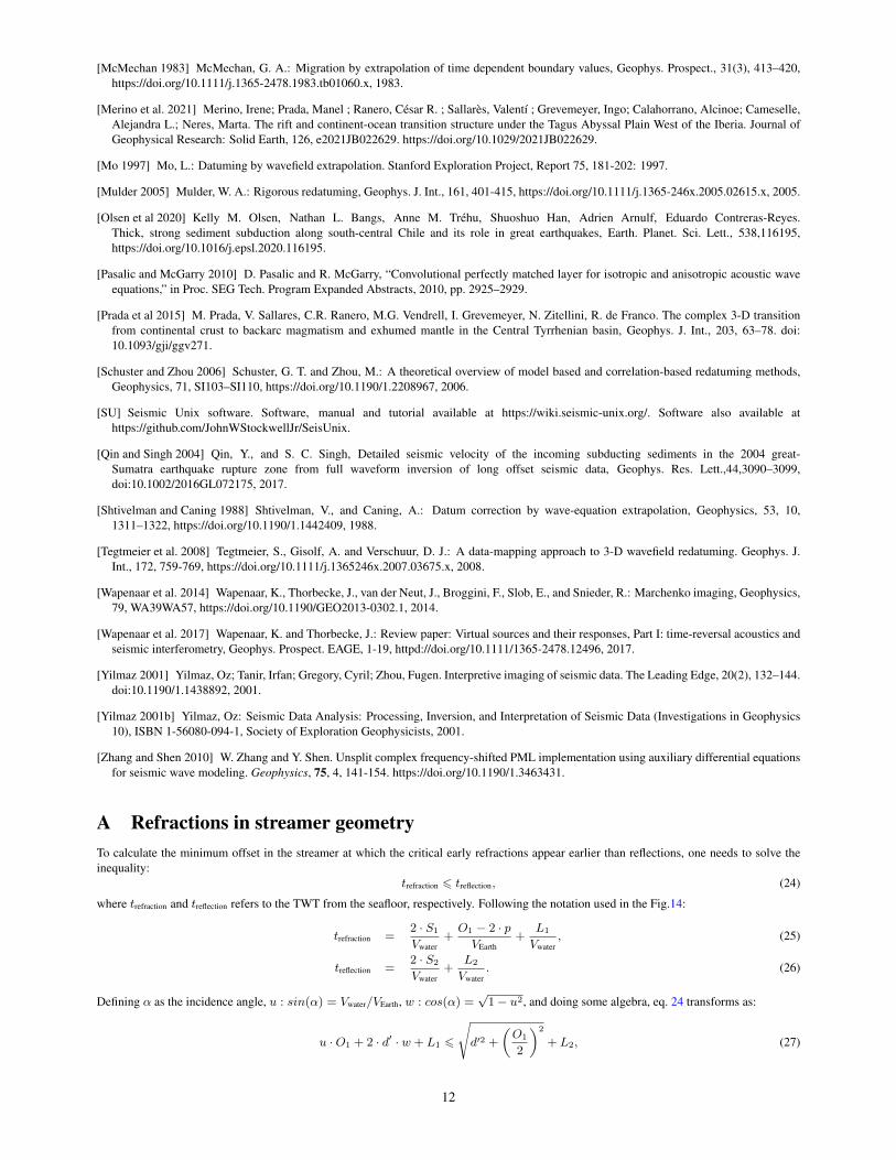
3.4.1 Well-suited case: TopoMed experiment

The TopoMed field data records were collected with the acquisition parameters shown in the first column of Tab. 3. The ratio between thestreamer length and the water column depth is n = SL

D = 3.7, and, as shown in Fig. 4-d), it is an efficient ratio that allows to record refractions in atleast 50%-75% of the total streamer length. The synthetic test using the TopoMed 1D-depth profile, Fig 8 (left panels), shows that the maximumoffset in the DC-redatumed shot gather coincides with the range of Vp values provided in Fig. 4, around 4.4 km in panel c2). Similarly for thefield data in Fig. 8 (panels d-e-f), the virtual redatumed shot gathers transform according to the geometries 1 and 2, showing the critical offsetaround 4.4 km as well (panel f). We clarify that the synthetic and field data cases shown together in Fig. 8, to compare the maximum criticaloffsets in the virtual geometry 1 results (panels b2 and e) and virtual geometry 2 results (panels c2 and f).

3.4.2 Poorly-suited case: Frame experiment

Second column of Tab. 3 shows the acquisition geometry of the FRAME experiment. In this case, the ratio between the streamer length and thewater column depth is n = 1.2 (see panel d, Fig 4), which indicates a very poor efficiency to register refractions in the streamer and therefore thisportends a bad functioning of the redatuming algorithm. The synthetic test using the model defined with the Frame 1D-depth profile is shownin Fig. 9 (left panels). The simulated and redatumed shot gathers in the geometry 1 in panels b1) and b2) are only coincident up to 3 km offset(yellow dashed line). This confirms that the refractions in streamer geometry can only be recorded from 6 km onwards and that the averagevelocity of the recorded waves is below 3 km/s. This means that there are no refractions originally recorded in the streamer and therefore onlyreflections are properly redatumed up to the maximum offset in geometry 1. Regarding the geometry 2 in panels c1) and c2), it is apparent thatthe results only show the propagation tails. Furthermore, the field data redatuming shown in panels e) and f) fails in the same manner too. Wecan conclude that for marine settings in which the water column depth is 5 km, streamer lengths of at least 10 km should be used (n = 2) if weaim at recording refractions as first arrivals.

8

3.5 Other relevant aspects3.5.1 Water column modelling

For simplicity, in all the tests shown above, the water layer is defined using an homogeneous value for the velocity model Vwater = 1500 m/s.However sea water P-wave velocity commonly ranges between 1520 m/s and 1450 m/s. Due to the fact that the DC algorithm presented inthis work is based on the 2-way wave equation, it is important to understand the influence of the water layer modelling on the streamer datapropagation. As an example, we show in panels a) and b) of Fig. 10, XBT data collected for salinity and temperature at an specific point inthe Atlantic Ocean (37◦30’N,12◦30’W) where the seafloor reaches 5 km depth. The panel c) of the same figure displays the P-wave velocitycalculated using the Mackenzie empirical equation ( Mackenzie 1981) (solid black line), which depends on the depth, salinity and temperature.The dashed blue line indicates the averaged velocity from the sea-surface till each specific depth. It is easy to see that this line oscillates around1511 m/s.

In Fig. 11 the TWT misfit is calculated between the true and synthetic water models, for the reflections and refractions from the seafloor.The TWT misfits, taking into account the equations 25 for refractions and 26 for reflections, are defined as:

∆TWTrefraction = |ttruerefraction − tsynth

refraction|, (21)

∆TWTreflection = |ttruereflection − tsynth

reflection| (22)

The propagation in the true water model (black solid line in panel c of Fig.10), is compared to two different homogenous synthetic models;the default value in most of the studies, 1500 m/s, and the averaged value for this particular setting, 1511 m/s. The TWT misfit for reflections(panels a and b) is shown for different offsets (x-axis) and seafloor depths (y-axis). The panel a) shows the misfit between the true modeland the synthetic one with Vwater = 1500 m/s, and similarly in panel b) but for the synthetic model with Vwater = 1511 m/s. Also, the TWTmisfit for seafloor refractions is shown at the lower panels (c and d), but in this case the x-axis indicates the P-wave velocity of the subsurface,VEarth. The most important observation is that when using a constant velocity model outside the true velocity ranges, the error can reach theorder of 0.1 second (2% in this example). However, if using a suitable P-wave velocity value, the propagation error becomes negligible (0.5%).Although the algorithm is prepared also to read real data from XBT measurements, for simplicity reasons and on those cases where marinefield data is not available, we recommend to use a realistic constant water velocity value.

3.5.2 Seafloor slope

The DC algorithm presented can read a specific bathymetry file with any seafloor relief and slope. It is important to note that the shotgatherredatuming will be successful only if enough refractions are recorded in the original field data, and this mainly depends on the water columndepth, subsurface velocity and streamer length. When the seafloor slope is pronounced, it is convenient to take it into account to properlypredict the critical offset. The equation 35 in Appendix A, gives the exact prediction for the minimum offset depending on the tilted angle ofthe seafloor, φ. To understand the effects of the slope of the recorded streamer data, we compute the error formula:

Error =

∣∣∣∣Offsetmin(φ)− Offsetmin(0)

Offsetmin(0)

∣∣∣∣ . (23)

This formula is interpreted as the error for the prediction of the minimum refraction offset in streamer data, when the seafloor is assumed tobe flat and the slope angle ignored. Fig. 12 shows as an example of the error(%) depending on the subsurface velocity (x-axis) and the slopeangle φ (y-axis) for an experimental situation in which Ds < Dr (Eq.35, appendix A). The top limit for the tilted angle is set to 20º which is arealistic upper limit for many submarine slopes (Harders et al. 2011). It is easy to see that for angles, φ < 10º, the total segment of the recordedrefractions varies less than 15% with respect to that recorded for flat surfaces. Therefore, the prediction for φ = 0º is a good first approximationto evaluate field data refractions in common marine scenarios.

3.5.3 Streamer data with poor acquisition geometry

The same test shown for the Marmousi model in Fig. 6 is repeated here, but to simulate legacy field data, where shot point distance is 100 mand receiver distance 50 m. The challenge for the redatuming algorithm is bigger in this case, as there is less data available due to the sparseacquisition geometry. In Fig. 13, we plot only the results obtained after redatuming the shotgather to geometry 2. As expected, the signal tonoise ratio is poor (panel a), and aliasing noise is apparent. However, if the original shot gathers are interpolated to halve shot point and receiverdistance before the redatuming, the signal to noise ratio improves (panel b).

4 DiscussionThis work addresses the performance and scope of a redatuming procedure based on the two-way wave equation. The redatuming transformsthe streamer field data simulating a virtual seafloor acquisition instead of the real sea surface one, removing the water column from the data. Inthe particular case of the early refractions, they transform as first arrivals. This provides the advantage to visualize originally hidden recordedrefractions, becoming distinguishable as first arrivals in the final virtual configuration. In that respect, the characterization of field data assuitable or unsuitable for redatuming depends on the amount of refractions recorded, as shown in the tests. The recorded length depends on theratio between the streamer length and the seafloor depth, the subsurface velocity and the seafloor slope.

The quantification of early refractions is central for this analysis due to their importance for building robust velocity models. Besides, itis also the best marker to verify the reliability of the virtual shot gathers and to quantify the maximum offset in all cases. This is possiblethanks to the availability of the seafloor bathymetry and the water velocity model, in contrast to the subsurface structure. We have shown thatthe redatumed results are a space-time transformation of the recorded field data. In this respect, the redatuming does not increase the amount

9

of information at long offsets as if the shot had directly been recorded on the seafloor. For this reason, it is essential to determine as good aspossible the maximum reliable offset in the redatumed virtual geometry.

The tests using benchmark models helps to understand that the first point (time and offset distance) where seafloor refractions are recordedin the streamer is the actual starting point of the redatumed shotgather in geometry 2. The first arrivals in this virtual geometry 2 form a linewith a slope equal to the value of the velocity of those layers where the refractions travelled, i.e. near offsets register refractions from theshallowest parts of the subsurface and the far offsets from deeper parts.

Regarding the reflections from the different subsurface layers, the tests with the benchmark model with two subsurface layers (see Supple-mentary Material) show that the transformation is also suitable up to the maximum offset in virtual geometry 2, whenever the reflection hasbeen previously recorded in the streamer.

With respect to the phase discrepancy of the redatumed results due to the usage of the DC method, is a predictable parameter in geologicalmodels with smooth gradient variations, and therefore straightforward to apply to the redatumed results. In the case of realistic scenarios, wherethe models can be very complex and non smooth, the estimation of phase discrepancies is not so straightforward (see Supplementary Material).Although more tests are needed in this respect, we have observed that this discrepancy is hardly greater than 0.05 seconds.

It is also noticeable the poor transformation of the resultant direct wave traveling through the water layer in the final redatumed shot gathers(see Figs. 2, 6, 8, 9 and figures displayed in the Supplementary Material). In this case, the original wave in the streamer data which transformsas the direct wave through the water in the final redatumed shot gather corresponds to waves traveling within the water column. As in thecase of refractions, and given a specific geological scenario, this offset increases using longer streamers. However, the offset of the properlytransformed direct wave is always shorter than the offset of the properly transformed refractions, and this would be a problem in the case ofneeding to use the full waveform in the virtual geometry 2.

In this way, although the arrival times in the virtual shot gather and also the reflections are predictable and their reliability easy to quantify,it is not straightforward to understand and control all the details related to the entire waveform. Taking all these aspects into account and theanalysis presented in Fig. 4, the best field data candidates to be redatumed to the seafloor are those recorded with streamer lengths two or threetimes the seafloor depth, and with an average P-wave velocity of the subsurface of VEarth > 3 km/s. Under these conditions, refractions can berecovered in 50% to 90% of the streamer length.

The redatuming procedure in this work is based on wave propagation throughout the water column, and in this sense the algorithm ismodel-dependent. However, as the model refers only to the sea water, where the velocity variation oscillates in a relatively small range ofvelocity values (< 70 m/s), the absence of detailed information from the water layer is not a drawback to obtain reliable results. If the watercolumn is characterized with a constant but realistic value for the velocity model, the estimated error at a specific offset for reflections andrefractions is negligible, from 0.5% to 2%, compared to the value obtained using the real water velocity model.

With respect to noise produced by data aliasing, it is a natural sub-product of the redatuming. The approach to minimise it is datainterpolation that increases signal to noise ratio attenuating aliasing noise.

5 Conclusion• We present and provide an easy-to-use open source software that enables the redatuming of 2D streamer data to the seafloor.

• It is a HPC-based code, therefore for an optimal computing time performance it should operate on a cluster.

• The input field data is required in SU format, which is a common format to store seismic data.

• Not all field data are suitable to be redatumed, it depends on the amount of refractions originally registered in the streamer. We providea suit of analytical formulas and assessment visual tools to estimate the suitability of a given data set to perform DC. We show that thisdepends on the streamer length, seafloor depth, subsurface P-wave velocity and seafloor slope.

• After applying the DC algorithm the refracted arrivals recorded in the streamer appear as first arrivals from nearly zero offset, so that theyare straightforward to pick. This is the main advantage taking into account that a considerable amount of the refractions are screened byreflections and noise in the original streamer recordings.

• Apart from the first arrival picking, it is also possible to use the reflection information. However, the waveforms are affected by theredatuming process, so their use is not straightforward.

• The absence of a detailed velocity model of the water layer is not an impediment to obtain reliable results.

• For legacy data recorded with poor acquisition geometry, narrowing the acquisition mesh allows the correct redatuming improving thedata contrast and avoiding aliasing noise. This would give a second chance to many past experiments with relevant information in areaswhere no new data is available.

6 Code availabilityThe DC code is available online at GitHub repository: https://github.com/ejimeneztejero/DC, under the GNU general public license v3.0.

AcknowledgmentsThis is a contribution of the Barcelona Center for Subsurface Imaging. The work has been partially supported by project FRAME with referenceCTM2015-71766-R, funded by the Spanish Ministry of Science, Innovation and Universities. ICM has also had funding support of the ‘SeveroOchoa Centre of Excellence’ accreditation (CEX2019-000928-S), of the Spanish Research Agency (AEI).

10

References[Audhkhasi and Singh 2019] Audhkhasi, P., and Singh, S. C. (2019).Seismic structure of the upper crust from 0-75 Ma in the equa-

torial atlantic ocean on the African plate using ultra-long offset seismic data. Geochemistry, Geophysics, Geosystems, 20, 6140,https://doi.org/10.1029/2019GC008577.

[Arnulf et al. 2011] Arnulf, A. F., Singh, S. C., Harding, A. J., Kent, G. M., and Crawford, W. C.: Strong seismic heterogeneity in layer 2Anear hydrothermal vents at the Mid-Atlantic Ridge, Geophys. Res. Lett., 38, L13320, https://doi.org/10.1029/2011GL047753, 2011.

[Barison et al. 2011] Barison, E., Brancatelli, G., Nicolich, R., Accaino, F., Giustiniani, M. and Tinivella, U.:Wave equa-tion datuming applied to marine OBS data and to land high resolution seismic profiling, J. Appl. Geophys.,73, 267-277,https://doi.org/10.1016/j.jappgeo.2011.01.009, 2011.

[Berkhout 1981] Berkhout, A. J.: Wavefield extrapolation techniques in seismic migration, a tutorial, Geophysics, 46, 1638–1656,https://doi.org/10.1190/1.1441172, 1981.

[Berkhout 1997a] Berkhout, A. J.: Pushing the limits of seismic imaging. Part I: prestack migration in terms of double dynamic focusing,Geophysics, 62(3), 937–953, https://doi.org/10.1190/1.1444201, 1997a.

[Berkhout 1997b] Berkhout, A. J.: Pushing the limits of seismic imaging. Part II: integration of prestack migration, velocity estimation, andAVO analysis, Geophysics, 62(3), 954–969, https://doi.org/10.1190/1.1444202, 1997b.

[Berryhill 1979] Berryhill, J. R.: Wave-equation datuming, Geophysics, 44, 13291344, https://doi.org/10.1190/1.1441010, 1979.

[Berryhill 1984] Berryhill, J. R.: Wave-equation datuming before stack, Geophysics, 49, 2064–2066, https://doi.org/10.1190/1.1441620, 1984.

[Bevc 1997] Bevc, D.: Flooding the topography: wave-equation datuming of land data with rugged acquisition topography, Geophysics, 62,1558-1569, https://doi.org/10.1190/1.1885634, 1997.

[Booth-Rea et al. 2007] Booth-Rea, G., Ranero, C. R., Martınez-Martınez, J. M., and Grevemeyer, I.: Crustal types and Tertiary tectonicevolution of the Alboran sea, western Mediterranean, Geochem. Geophys. Geosyst., 8, 1525–2027, https://doi.org/10.1029/2007GC001639,2007.

[Booth-Rea et al. 2018] Booth-Rea, G., Ranero, C. R., and Grevemeyer, I.: The Alboran volcanic-arc modulated the Messinian faunal ex-change and salinity crisis, Sci. Rep.-UK, 8, 13015, https://doi.org/10.1038/s41598-018-31307-7, 2018.

[Gras et al. 2019] Gras C., Dagnino D., Jimenez-Tejero C.E., Melendez A., Sallares V. and Ranero C.. Full-waveform inversion of short-offset,band-limited seismic data in the Alboran Basin (SE Iberia). Solid Earth, 10, 1833–1855, 2019 https://doi.org/10.5194/se-10-1833-2019.

[Gras et al. 2021] C. Gras, C. E. Jimenez-Tejero, V. Sallares, A. Melendez and C. R. Ranero, ”Toward a Practical Appraisal for WaveformTomography of Band- and Offset-Limited Marine Seismic Data,” in IEEE Transactions on Geoscience and Remote Sensing, vol. 60, pp.1-14, 2022, Art no. 4504814, doi: 10.1109/TGRS.2021.3097966.

[Cho et al. 2016] Cho, Y., Ha, W., Kim, Y., Shin, S., and Park, E.: Laplace-FourierDomain Full Waveform Inversion of Deep-Sea SeismicData Acquired with Limited Offsets, Pure Appl. Geophys., 173, 749773, https://doi.org/10.1007/s00024-015-1125-7, 2016.

[Claerbout 1976] Claerbout, J. F.: Fundamentals of Geophysical Data Processing, McGraw-Hill Inc., New York, 1976.

[Claerbout 1985] Claerbout, J.F.: Imaging the Earth’s Interior, Blackwell Scientific Publications, Oxford, 414pp, 1985.

[Gary S. Martin et al. 2006] Gary S. Martin, Robert Wiley, Kurt J. Marfurt; Marmousi2 : An elastic upgrade for Marmousi. The Leading Edge2006;; 25 (2): 156–166. doi: https://doi.org/10.1190/1.2172306.

[Gazdag 1978] Gazdag, J.: Wave equation migration with the phase-shift method, Geophysics, 43, 13421351,https://doi.org/10.1190/1.1440899, 1978.

[Harding et al. 2016] Harding, A. J., Arnulf, A. F., and Blackman, D. K.: Velocity structure near IODP Hole U1309D, AtlantisMassif, from waveform inversion of streamer data and borehole measurements. Geochem. Geophys. Geosyst., 17, 1990–2014,https://doi.org/10.1002/2016GC006312, 2016.

[Harders et al. 2011] Harders, R., Ranero, C. R., Weinrebe, W., & Behrmann, J. H. (2011). Submarine slope failures along the convergentcontinental margin of the Middle America Trench. Geochemistry, Geophysics, Geosystems, 12(6).

[ Mackenzie 1981] K.V. Mackenzie, Nine-term equation for the sound speed in the oceans (1981) J. Acoust. Soc. Am. 70(3), 807-812.https://doi.org/10.1121/1.386920.

[Marjanovic et al. 2017] Marjanovic, M., Fuji, N., Singh, S. C., Belahi, T., and Escartın, J. (2017). Seismic signatures of hydrothermalpathways along the East Pacific Rise between 9◦16’ and 9◦56’N. Journal of Geophysical Research: Solid Earth, 122, 10, 241-10, 262.https://doi.org/10.1002/2017JB015004.

[McMechan 1982] McMechan, G. A.: Determination of source parameters by wavefield extrapolation, Geophys. J. Roy. Astr. S., 71, 613–628,https://doi.org/10.1111/j.1365-246X.1982.tb02788.x, 1982.

11

[McMechan 1983] McMechan, G. A.: Migration by extrapolation of time dependent boundary values, Geophys. Prospect., 31(3), 413–420,https://doi.org/10.1111/j.1365-2478.1983.tb01060.x, 1983.

[Merino et al. 2021] Merino, Irene; Prada, Manel ; Ranero, Cesar R. ; Sallares, Valentı ; Grevemeyer, Ingo; Calahorrano, Alcinoe; Cameselle,Alejandra L.; Neres, Marta. The rift and continent-ocean transition structure under the Tagus Abyssal Plain West of the Iberia. Journal ofGeophysical Research: Solid Earth, 126, e2021JB022629. https://doi.org/10.1029/2021JB022629.

[Mo 1997] Mo, L.: Datuming by wavefield extrapolation. Stanford Exploration Project, Report 75, 181-202: 1997.

[Mulder 2005] Mulder, W. A.: Rigorous redatuming, Geophys. J. Int., 161, 401-415, https://doi.org/10.1111/j.1365-246x.2005.02615.x, 2005.

[Olsen et al 2020] Kelly M. Olsen, Nathan L. Bangs, Anne M. Trehu, Shuoshuo Han, Adrien Arnulf, Eduardo Contreras-Reyes.Thick, strong sediment subduction along south-central Chile and its role in great earthquakes, Earth. Planet. Sci. Lett., 538,116195,https://doi.org/10.1016/j.epsl.2020.116195.

[Pasalic and McGarry 2010] D. Pasalic and R. McGarry, “Convolutional perfectly matched layer for isotropic and anisotropic acoustic waveequations,” in Proc. SEG Tech. Program Expanded Abstracts, 2010, pp. 2925–2929.

[Prada et al 2015] M. Prada, V. Sallares, C.R. Ranero, M.G. Vendrell, I. Grevemeyer, N. Zitellini, R. de Franco. The complex 3-D transitionfrom continental crust to backarc magmatism and exhumed mantle in the Central Tyrrhenian basin, Geophys. J. Int., 203, 63–78. doi:10.1093/gji/ggv271.

[Schuster and Zhou 2006] Schuster, G. T. and Zhou, M.: A theoretical overview of model based and correlation-based redatuming methods,Geophysics, 71, SI103–SI110, https://doi.org/10.1190/1.2208967, 2006.

[SU] Seismic Unix software. Software, manual and tutorial available at https://wiki.seismic-unix.org/. Software also available athttps://github.com/JohnWStockwellJr/SeisUnix.

[Qin and Singh 2004] Qin, Y., and S. C. Singh, Detailed seismic velocity of the incoming subducting sediments in the 2004 great-Sumatra earthquake rupture zone from full waveform inversion of long offset seismic data, Geophys. Res. Lett.,44,3090–3099,doi:10.1002/2016GL072175, 2017.

[Shtivelman and Caning 1988] Shtivelman, V., and Caning, A.: Datum correction by wave-equation extrapolation, Geophysics, 53, 10,1311–1322, https://doi.org/10.1190/1.1442409, 1988.

[Tegtmeier et al. 2008] Tegtmeier, S., Gisolf, A. and Verschuur, D. J.: A data-mapping approach to 3-D wavefield redatuming. Geophys. J.Int., 172, 759-769, https://doi.org/10.1111/j.1365246x.2007.03675.x, 2008.

[Wapenaar et al. 2014] Wapenaar, K., Thorbecke, J., van der Neut, J., Broggini, F., Slob, E., and Snieder, R.: Marchenko imaging, Geophysics,79, WA39WA57, https://doi.org/10.1190/GEO2013-0302.1, 2014.

[Wapenaar et al. 2017] Wapenaar, K. and Thorbecke, J.: Review paper: Virtual sources and their responses, Part I: time-reversal acoustics andseismic interferometry, Geophys. Prospect. EAGE, 1-19, httpd://doi.org/10.1111/1365-2478.12496, 2017.

[Yilmaz 2001] Yilmaz, Oz; Tanir, Irfan; Gregory, Cyril; Zhou, Fugen. Interpretive imaging of seismic data. The Leading Edge, 20(2), 132–144.doi:10.1190/1.1438892, 2001.

[Yilmaz 2001b] Yilmaz, Oz: Seismic Data Analysis: Processing, Inversion, and Interpretation of Seismic Data (Investigations in Geophysics10), ISBN 1-56080-094-1, Society of Exploration Geophysicists, 2001.

[Zhang and Shen 2010] W. Zhang and Y. Shen. Unsplit complex frequency-shifted PML implementation using auxiliary differential equationsfor seismic wave modeling. Geophysics, 75, 4, 141-154. https://doi.org/10.1190/1.3463431.

A Refractions in streamer geometryTo calculate the minimum offset in the streamer at which the critical early refractions appear earlier than reflections, one needs to solve theinequality:

trefraction 6 treflection, (24)

where trefraction and treflection refers to the TWT from the seafloor, respectively. Following the notation used in the Fig.14:

trefraction =2 · S1

Vwater+O1 − 2 · pVEarth

+L1

Vwater, (25)

treflection =2 · S2

Vwater+

L2

Vwater. (26)

Defining α as the incidence angle, u : sin(α) = Vwater/VEarth, w : cos(α) =√

1− u2, and doing some algebra, eq. 24 transforms as:

u ·O1 + 2 · d′ · w + L1 6

√d′2 +

(O1

2

)2

+ L2, (27)

12

where

d′ = d · cosφ, (28)

O1 =Offset · cosφ · (w − u · tanφ)

w, (29)

L1 =Offset · sinφ

w, (30)

O2 =2 · d · cosφ

2 · d+ Offset · tanφ, (31)

L2 = Offset · sinφ ·√

1 +

(Offset

2 · d+ Offset · tanφ

)2

. (32)

and φ is the subfloor slope. Solving eq.27, the offset minimum at which refractions appear earlier than reflexions is:

OffsetStreamermin =

2 · d · u · (w − u · tanφ)

u2 · (tan2 φ− 1)− 2 · u · w · tanφ+ 1. (33)

For any type of marine setting, and eliminating the explicit dependence on Dr as:

Dr = Ds + Offset · tanφ · Sign · [Dr −Ds], (34)

The solutions for the minimum offset with refractions, depending on the marine setting type is:

OffsetStreamermin =

Ds ·G(φ) if Ds < Dr, (φ > 0)

Ds·G(φ)1+G(φ)·tanφ

if Ds > Dr, (φ > 0)

Ds ·G(0) if Ds = Dr, (φ = 0)

(35)

where

G(φ) =

2·u·(w−u·tanφ)

u2·(tan2 φ−1)−2·u·w·tanφ+1if φ > 0

2·uw

if φ = 0

(36)

B Refractions in geometry 1For the geometry 1 or OBS geometry (sources at the sea surface and receivers at the seafloor), and following the notation of Fig.14, the TWTrefraction and reflection arrivals are:

trefraction =S1

Vwater+

Offset’− p+ q

VEarth, (37)

treflection =S2

Vwater. (38)

(39)

Defining u : sin(α) = Vwater/VEarth and w : cos(α) =√

1− u2, and doing some algebra, the equation to solve, taking into account Eq. 24, is:

d′ + u · (O · w − u · d′) 6 w ·√d′2 + O2 (40)

where

d′ = d · cosφ, (41)

O = Offset · cosφ+ d · sinφ. (42)

(43)

The solution for the minimum offset with refractions in this specific configuration is:

OffsetGeom1min = d · u

w−D tanφ, (44)

and the general solution at any marine setting, and taking into account Eq. 34, is:

OffsetGeom1min =

Ds·( uw−tanφ)

1+tan2 φif Ds < Dr, (φ > 0)

Ds·( uw

+tanφ)1+tan2 φ

if Ds > Dr, (φ > 0)

Ds · uw if Ds = Dr, (φ = 0)

(45)

13

DC of streamer field data

Figure 1: DC redatuming applied to field data recorded on TopoMed experi-ment ((Booth-Rea et al. 2007), (Booth-Rea et al. 2018)). For this experiment and location, the streamer length and thewater depth are 6 km and 1.6 km, respectively. Panel a) streamer shot gather. Panel b) the shot gather in panel a) redatumed toacquisition geometry 1. Panel c) the shot gather in panel a) redatumed to the seafloor, or acquisition geometry 2.

14

Offsetmin

Offsetmin Offsetmin

Offsetmax

Offsetmax

DC synthetic test: benchmark model

Figure 2: DC redatuming of a streamer shot gather to the seafloor using a synthetic model with VEarth= 3 km/s and 2 km waterdepth. The dashed blue line indicate the minimum offset at which early refractions are registered as first arrivals in the streamer(and geometry 1) configuration and the dashed yellow and red lines point at the maximum offset in the virtual redatumed shotgathers (to geometry 2) where the first arrivals are truncated. Following equation 5 in the Supplementary Material, a phasecorrection of 0.0317 seconds has been applied to the redatumed result in geometry 2.

15

km

Figure 3: Minimum offset (see Eq. 15), at which the refractions are registered in a shot gather with streamer acquisition geometry,for a flat seafloor (φ = 0). The x-axis displays the seafloor velocity in the benchmark models from 2 and 5 km/s and the y-axisthe water column depth between 0.5 to 6 km.

16

0 1 2 3 4 5 6 7 8 9 10 11 12n = SL / D

0

25%

50%

75%

100%

Offs

etm

ax(%

)

VEarth = 2 km/sVEarth = 2.5 km/sVEarth = 3 km/sVEarth = 3.5 km/sVEarth = 4 km/sVEath = 4.5 km/sVEarth = 5 km/s

d)

Maximum offset in redatumed shot gathers (Geometry 2)

km km km

Figure 4: Maximum offset in virtual redatumed shot gathers, OffsetGeom2max , where first arrivals are truncated. Upper panels:

maximum offset for different streamer lengths (SL) of a) 3 km, b) 6 km and c) 10 km. The x-axis displays the seafloor velocityin the benchmark models from 2 to 5 km/s and the y-axis the water column depth from 0.5 to 6 km. Lower panel d: diagramwhich summarizes the three upper panels into one. Here the maximum offset is expressed as a percentage (%) of the total length(y-axis) depending on the rate n = SL

D (x-axis), which compares the size of the streamer (SL) with the water column depth (D).Every line refers to an specific P-wave velocity of the subsurface, VEarth.

1,5 2 2,5 3 3,5 4 4,5 5Vp (km/s)

0

1

2

3

4

Dep

th (k

m)

a) Marmousi model b) Vp-depth profile

km/s

Figure 5: a) Synthetic Marmousi model with a 1 km water column. The Marmousi model has been re-dimension for this testto the following proportions, 19 km length x 4 km depth. The black line located at around 12 km distance indicates de positionat which we show the depth profile in panel b), which is also the position of the shot gather shown in Fig. 6. b) Velocity-depthprofile at the specific location indicated in panel a) with a black arrow.

17

Offsetmax

Offsetmax

DC synthetic test: Marmousi model

Figure 6: Redatuming synthetic test using the Marmousi model shown in Fig. 5. Panel a) displays an streamer shot gathergenerated at the location indicated with a black arrow in Fig. 5. Panel b1 and b2 show the shot gather generated in geometry 1and the virtual redatumed result of panel a) into geometry 1, respectively. Similarly, panels c1 and c2 show the same as the panelsabove but for the geometry 2. The yellow dashed line in panel b2) indicate the maximum critical offset for the first arrivals beforedata are truncated in the virtual geometry 1. The same for panel c2 but for the virtual geometry 2.

18

Profile TopoMeda1) TopoMed model

2 3 4 5 6 7 8P-waves seismic velocity (km/s)

34

55 5

66 6

77

88

6

8

66 6 66.5

6.5777.57.5

7.5 7.5

0

10

20

Dep

th (k

m)

25 50 75 100 125 150 175 200 225 250 275 300 325 350 375 400 425 450

Distance (km)

0

10

20

Dep

th (k

m)

25 50 75 100 125 150 175 200 225 250 275 300 325 350 375 400 425 450Distance (km)

10−2 101 102 103

Derivative Weight Sum

747372 71 69686766656463626160 58 57565554 5251504948474645 107 108 109 110

Profile Frameb1) Frame model

a2) Vp-depth profile TopoMed

1,5 2 2,5 3 3,5 4Vp (km/s)

0

1

2

3Dep

th (k

m)

1,5 2 2,5 3 3,5 4 4,5Vp (km/s)

01234567

Dep

th (k

m)

b2) Vp-depth profile Frame

Figure 7: Field data cases. Vp tomographic models obtained with travel-time tomography for the experiments a1) TopoMed(Gras et al. 2019) and b1) Frame (? ). The black and red arrows indicate the location of the depth-profile shown in panels a2 andb2.

19

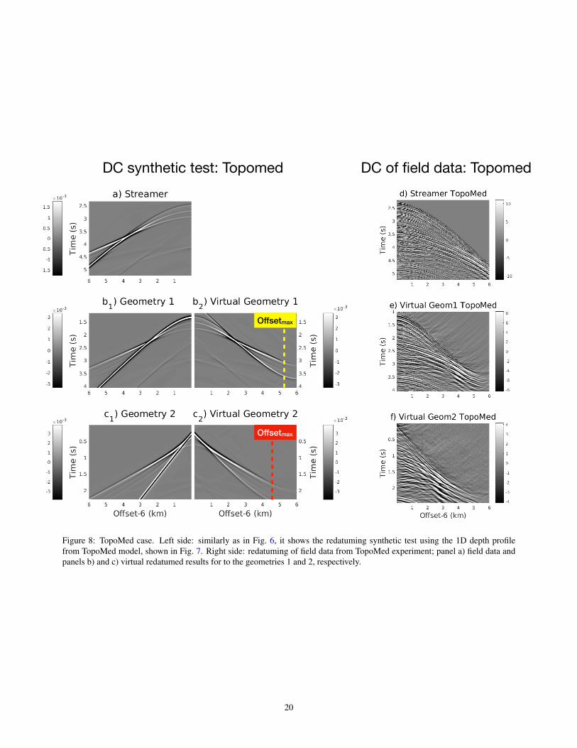
DC synthetic test: Topomed DC of field data: Topomed

Offsetmax

Offsetmax

Figure 8: TopoMed case. Left side: similarly as in Fig. 6, it shows the redatuming synthetic test using the 1D depth profilefrom TopoMed model, shown in Fig. 7. Right side: redatuming of field data from TopoMed experiment; panel a) field data andpanels b) and c) virtual redatumed results for to the geometries 1 and 2, respectively.

20

Offsetmax

DC synthetic test: Frame DC of field data: Frame

Figure 9: Frame case. Left side: similarly as in Figs. 6 and 8, it shows the redatuming synthetic test using the 1D-depth profilefrom Frame model, shown in Fig. 7. Right side: redatuming of field data from Frame experiment; panel a) field data and panels b)and c) virtual redatumed results for to the geometries 1 and 2, respectively.

21

34,5 35 35,5 36 36,5S (ppt)

0

1

2

3

4Dep

th (k

m)

a) Salinity

0 5 10 15 20T (ºC)

0

1

2

3

4

b) Temperature

1,5 1,52 1,54Vwater (km/s)

0

1

2

3

4

c) Water velocity

Average velocityat each depth

Figure 10: An example of a) salinity, b) temperature and c) P-wave velocity of the water column. The data for the salinity andtemperature are taken from XBT measurements at an specific location in the Atlantic ocean (37◦30’N,12◦30’W). The P-wavevelocity (black line in panel c) is calculated using the Mackenzie empirical equation ( Mackenzie 1981). The dashed blue line inpanel c) is the average velocity calculated with the velocity values from the sea surface till each specific depth.

seconds

Refractions Refractions

Reflections Reflections

seconds

Figure 11: Panels a) and b) show the TWT misfit for seafloor reflections, and panels c) and d) for seafloor refractions, both forφ = 0. The panels on the left (a and c) compute the misfit between the ’true’ water column shown in Fig. 11 and a homogeneouswater column with Vwater = 1500 m/s. Similarly in the right panels (b and d) but using for the homogeneous water column theaverage value of velocity Vwater = 1511 m/s.

22

%

Figure 12: Error (%) of the critical minimum offset to register refractions depending on the P-wave velocity of the subsurface(x-axis) and the angle of the seafloor slope φ() (y-axis). The error formula is computed with eq. 23.

Figure 13: Synthetic test simulating legacy field data with a poor streamer acquisition geometry (dshots = 100m, drec = 50m)and using the Marmousi model (Fig. 5). Panel a) shows the virtual DC redatumed shot gather for the poor acquisition geometry,which evidence a very low signal to noise ratio. In panel b), the signal to noise ratio is clearly improved by interpolating theoriginal streamer shot gathers to a narrower mesh before applying the DC-algorithm as (dshots = 50m, drec = 12.5m).

23

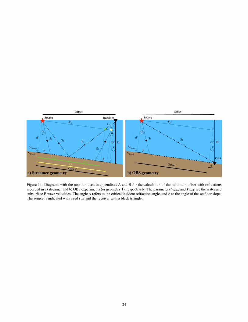
Offset’

p

L2L1

p

α α

O2/2O2/2

D’

O1

Offset

Receiver

.

.

Source

Vwater

VEarth

ϕ

S1

S2 S2

d’D

S1

ϕ

a) Streamer geometry

Offset’

d’

OBS

ϕ

q

.

.

Offset

p

ϕSource

S1 S2D’ D

α

Vwater

VEarth

b) OBS geometry

Figure 14: Diagrams with the notation used in appendixes A and B for the calculation of the minimum offset with refractionsrecorded in a) streamer and b) OBS experiments (or geometry 1), respectively. The parameters Vwater and VEarth are the water andsubsurface P-wave velocities. The angle α refers to the critical incident refraction angle, and φ to the angle of the seafloor slope.The source is indicated with a red star and the receiver with a black triangle.

24

Supplementary Material

Contents1 Phase conservation in the redatumed shotgathers 1

2 DC tests with Benchmark models 3

3 Two-layer models: reflections and secondary refractions 4

List of FiguresS1 First arrivals discrepancy in redatumed shotgathers . . . . . . . . . . 5S2 Trace comparison for simple benchmark models . . . . . . . . . . . . 6S3 First arrival comparison for simple benchmark models . . . . . . . . 7S4 Trace comparison for realistic models . . . . . . . . . . . . . . . . . 8S5 First arrival comparison for simple benchmark models . . . . . . . . 9S6 Synthetic test I: streamer length . . . . . . . . . . . . . . . . . . . . 10S7 Synthetic test II: water column depth . . . . . . . . . . . . . . . . . . 11S8 Synthetic test III: subsurface velocity . . . . . . . . . . . . . . . . . . 12S9 Synthetic test II: two-layers benchmark model . . . . . . . . . . . . . 13

1 Phase conservation in the redatumed shotgathersThe purpose of using the DC software is to provide shot gathers collected on a streamerredatumed to the seafloor. In this new datum is easier to visualize and map the recordedrefractions as first arrivals in order to invert them with travel-time tomography tech-niques and therefore obtaining velocity models from the subsurface. In this respect,the concern for the conservation of the full shot gather (amplitudes and phases) in theDC process is reduced to the suitable calculation of the phase, specifically of the firstarrival times.

We can define the phase error for the virtually redatumed shotgathers to geometry 2,as the difference between the expected phases of the shotgather directly generated withsources and receivers at the seafloor (tGeom2

0 ) and the original MCS shotgather virtuallyredatumed to the seafloor (tvGeom2

0 ). Using the DC methodology leads to this type ofsystematic error for the first arrivals, which mainly depends on the offset and the veloc-ity of the subsurface. This error can be estimated for the first receiver and added afteras a constant to correct the phases of the entire shotgather. The following expressionsare formulated assuming that source and receivers are located at the same depth posi-tion below the sea surface in the MCS experiment, and considering a flat seafloor. The

1

arX

iv:2

106.

0064

6v4

[ph

ysic

s.ge

o-ph

] 2

4 Fe

b 20

22

expected first arrival (direct ray) for the trace generated directly at the seafloor can beobtained as:

tGeom20 =

offsetVEarth

, (1)

where the offset parameter refers to the distance between the source and the receiverand VEarth to the average velocity of the path through which the direct ray has propa-gated in the subsurface. The expected first arrival of the original MCS trace virtuallyredatumed to the seafloor is:

tvGeom20 = tstreamer

0 − 2 · DVwater

, (2)

where D is the depth between the original source (or receivers at the streamer) andthe seafloor, and tstreamer

0 refers to the first reflected ray from the seafloor, propagatingfrom the source to the receiver:

tstreamer0 = 2 ·

√(offset/2)2 + D2

Vwater. (3)

Finally, the phase discrepancy can be estimated as :

Error[tvGeom20 ] = tGeom2

0 − tvGeom20 . (4)

This mismatch is plotted in Fig. S1, depending on the offset and VEarth parameters.The influence of the depth parameter in the result is not significant, and for this plotit has been fixed to 2 km. The phase correction to the redatumed shotgathers is alsoincluded as an option in the DC software, following the equation 4.

This phase correction has been successfully applied to the Benchmark tests to betterset the phase of the redatumed results to geometry 2. We show in Fig. S2, for twodifferent benchmark models with the same streamer length (6 km with 240 receivers),different examples of traces from the first receiver to the middle one (1st, 30th, 60th,90th and 120th). In each panel, three traces are compared; the synthetic trace directlygenerated at the seafloor (black solid line) and the trace result after applying the DCmethod (starting from the original trace in the streamer). The raw calculation is shownwith a red dashed line, and the result after correcting the phase discrepancy is shownwith a green dotted line. In these examples, the phase correction allows to properlyset the first arrival to the expected value. In figure S3 we show the whole length offirst arrival times up to the middle of the streamer (3 km), for both benchmark models(upper panels) and the phase error between the redatumed and expected results (lowerpanels).

In Figs. S4 and S5, we show a similar comparison but for two other synthetic mod-els; the marmousi model and the Topomed model (see manuscript). In both cases, thestreamer length is also 6 km, consisting of 480 receivers. The panels in Figs. S4 showthe comparison between traces from the first to the middle receiver (1st, 30th, 60th,120th, 240th) and Figs. S5 the length of first arrival times up the middle of the streamer(3 km).

The main conclusion of the tests is that the phase correction approximation is validand can be applied in geological scenarios with a smooth velocity gradient. In thecase of realistic scenarios, where the models can be very complex and non smooth,the estimation of phase discrepancies is not straightforward. In the examples shown in

2

the manuscript with the marmousi, topomed and frame model, the phase correction isnot applied to the redatumed results. However we have observed that this phase dis-crepancy is hardly greater than 0.05 seconds. Nevertheless, more tests using realisticexamples would be needed to analyze and estimate this discrepancy and its possiblypredictable behavior, depending on, for example, the velocity gradient of the subsur-face. Also, to study the effects that the usage of the virtual redatumed first arrivalswith no a priori phase correction would have on the final inverted velocity models afterapplying tomographic inversion techniques.

2 DC tests with Benchmark modelsIn this analysis, we present the different synthetic tests using the Benchmark models.A total set of 84 models are generated varying the following parameters:

• Water column depth, D, from 0.5 to 6 km, every 0.5 km.

• Constant subsurface p-wave velocity, VEarth, from 2 to 5 km/s, every 0.5 km/s.

The common features are:

• Flat seafloor surface.

• Constant water p-wave velocity, Vwater = 1.5 km/s.

To recreate realistic marine seismic acquisition experiments, we select three differ-ent cable lengths for the streamer in our tests; 3, 6 and 10 km. The advantage of usingshorter streamers (6 3 km) is that they can be deployed in areas with possible obsta-cles, providing a good control over the data. Streamers of 6 km length are the mostcommon ones and widely used in academy and industry research. Longer streamers of> 10 km length, mostly used in industry nowadays, provide information from deeperareas of the subsurface but greatly increase the cost and experimental requirements.

Concerning the main acquisition parameters, the simulation time is set to 10 sec-onds, the source is a ricker wavelet with central frequency of 10 Hz, the distance be-tween sources is 50 m and between receivers is 25 m, and three different streamerlengths are tested: 3, 6 and 10 km.

The figures S6, S7 and S8 show the virtual redatumed shotgathers to geometry 2depending on the streamer length (SL), the water column depth (D) and seafloor p-wavevelocity (VEarth), respectively. For space and clarity reasons, the results for the real andvirtual OBS configurations are omitted in these figures. First and second columns showthe shotgather directly simulated with streamer and geometry 2, and the third columnthe virtually redatumed shotgather from column 1 into geometry 2, respectively. InFig. S6, the parameters are set to D = 2 km and VEarth = 3 km/s and SL at each row is 3,6 and 10 km. As expected, the longer the streamer, the longer the offset with refractionsregistered. In Fig. S7 the fixed parameters are SL = 6 km and VEarth = 3 km/s and Dat each row is 1, 2 and 3 km, showing a inversely proportional decrease of refractionswith the increasing depth. Finally in Fig. S8, the fixed parameters are SL = 6 km andD = 2 km/s, with VEarth varying at each row with 2, 3 and 4 km/s. In this case, thehigher the velocity of the subsurface, the more refractions registered.

3

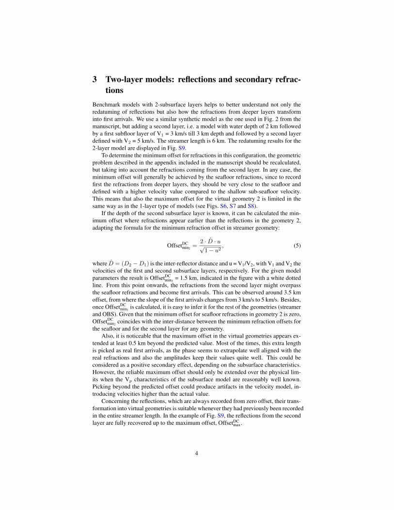
3 Two-layer models: reflections and secondary refrac-tions

Benchmark models with 2-subsurface layers helps to better understand not only theredatuming of reflections but also how the refractions from deeper layers transforminto first arrivals. We use a similar synthetic model as the one used in Fig. 2 from themanuscript, but adding a second layer, i.e. a model with water depth of 2 km followedby a first subfloor layer of V1 = 3 km/s till 3 km depth and followed by a second layerdefined with V2 = 5 km/s. The streamer length is 6 km. The redatuming results for the2-layer model are displayed in Fig. S9.

To determine the minimum offset for refractions in this configuration, the geometricproblem described in the appendix included in the manuscript should be recalculated,but taking into account the refractions coming from the second layer. In any case, theminimum offset will generally be achieved by the seafloor refractions, since to recordfirst the refractions from deeper layers, they should be very close to the seafloor anddefined with a higher velocity value compared to the shallow sub-seafloor velocity.This means that also the maximum offset for the virtual geometry 2 is limited in thesame way as in the 1-layer type of models (see Figs. S6, S7 and S8).

If the depth of the second subsurface layer is known, it can be calculated the min-imum offset where refractions appear earlier than the reflections in the geometry 2,adapting the formula for the minimum refraction offset in streamer geometry:

OffsetDCmin2

=2 · D · u√1− u2

, (5)

where D = (D2 −D1) is the inter-reflector distance and u = V1/V2, with V1 and V2 thevelocities of the first and second subsurface layers, respectively. For the given modelparameters the result is OffsetDC

min2= 1.5 km, indicated in the figure with a white dotted

line. From this point onwards, the refractions from the second layer might overpassthe seafloor refractions and become first arrivals. This can be observed around 3.5 kmoffset, from where the slope of the first arrivals changes from 3 km/s to 5 km/s. Besides,once OffsetDC

min2is calculated, it is easy to infer it for the rest of the geometries (streamer

and OBS). Given that the minimum offset for seafloor refractions in geometry 2 is zero,OffsetDC

min2coincides with the inter-distance between the minimum refraction offsets for

the seafloor and for the second layer for any geometry.Also, it is noticeable that the maximum offset in the virtual geometries appears ex-

tended at least 0.5 km beyond the predicted value. Most of the times, this extra lengthis picked as real first arrivals, as the phase seems to extrapolate well aligned with thereal refractions and also the amplitudes keep their values quite well. This could beconsidered as a positive secondary effect, depending on the subsurface characteristics.However, the reliable maximum offset should only be extended over the physical lim-its when the Vp characteristics of the subsurface model are reasonably well known.Picking beyond the predicted offset could produce artifacts in the velocity model, in-troducing velocities higher than the actual value.

Concerning the reflections, which are always recorded from zero offset, their trans-formation into virtual geometries is suitable whenever they had previously been recordedin the entire streamer length. In the example of Fig. S9, the reflections from the secondlayer are fully recovered up to the maximum offset, OffsetDC

max.

4

Error[t0vGeom2] (s)

1.5 2 2.5 3 3.5 4VEarth (km/s)

0.05

0.1

0.15

0.2

Nea

r off

set (

km)

0.02

0.04

0.06

0.08

0.1

0.12

s

Figure S1: Time error (in seconds) for the first arrival in the redatumed shotgathersto the seafloor (see equation 4), depending on the p-wave velocity of the earth surface(x-axis) and the near offset or distance between the source and the first receiver (y-axis). The depth is fixed to 2 km, however the phase error dependency with the depthis almost negligible.

5

0,1 0,2 0,3-0,05

00,05

A) Model 2 km/s, Depth 1 km

0,4 0,5 0,6 0,7 0,8-0,005

00,005

0,8 0,9 1-0,002

00,002

1,1 1,2 1,3-0,001

00,001

1,5 1,6 1,7 1,8Time (s)

-0,001

0

0,001

0,1 0,2 0,3-0,05

00,05

B) Model 3 km/s, Depth 2 km

0,2 0,3 0,4 0,5-0,002

00,002

0,5 0,6 0,7 0,8-0,001

0

0,001

0,8 0,9 1-0,001

0

0,001

1 1,1 1,2 1,3Time (s)

-0,00030

0,0003

a1) trace 1

a2) trace 30

a3) trace 60

a4) trace 90

a5) trace 120

b1) trace 1

b2) trace 30

b3) trace 60

b4) trace 90

b5) trace 120

Figure S2: Trace comparison for two of the benchmark models, both of them usingan streamer length of 6 km (240 receivers). Panels in the first column refer to A)benchmark model with VEarth = 2 km/s and water depth = 1 km/s, and those panelsin the second column refer to B) benchmark model with VEarth = 3 km/s and waterdepth = 2 km/s. Black solid lines are the traces synthetically generated directly in Ge-ometry 2, red dashed lines are the traces from the redatumed shotgather to Geometry 2,and green dotted lines are also the traces from the redatumed shotgather but correctedwith the error shown in Fig. S1. Following equation 4, this correction is 0.0483 secondsfor model A) and 0.0317 seconds for model B).

6

0 1 2 3

0

0,5

1

1,5

2

FA [s

]

Shot at Geom2 (true)Shot at vGeom2 (virtual)Corrected shot at vGeom2 (virtual)

A) Model 2 km/s, Depth 1 km

0 1 2 3

0

0,5

1

1,5

2

B) Model 3 km/s, Depth 2km

0 1 2 3Streamer length [km]

0

0,02

0,04

0,06

0,08

0,1

Erro

r [s]

0 1 2 3Streamer length [km]

0

0,02

0,04

0,06

0,08

0,1

Figure S3: First arrival (FA) comparison for two benchmark models. First row showsthe first arrivals for three shotgathers; the shotgather directly generated in geome-try 2 (black solid line), the virtual redatumed MCS shotgather to geometry 2 (reddashed line) and the redatumed one with the phase correction added (green dottedline). Second row shows the error between the first arrivals of the redatumed shotgath-ers and the synthetic one. Panels in the first column refer to A) benchmark model withVEarth = 2 km/s and water depth = 1 km/s, and those panels in the second column referto B) benchmark model with VEarth = 3 km/s and water depth = 2 km/s.

7

0,1 0,2 0,3 0,4-0,02

00,02

B) Topomed synthetic model, Depth 2 km

0,4 0,5 0,6-0,03

00,03

0,4 0,5 0,6 0,7-0,02

00,02

0,8 0,9 1 1,1-0,01

00,01

1,3 1,4 1,5Time (s)

-0,0030

0,003

0,1 0,2 0,3-0,1

00,1

A) Marmousi model, Depth 1 km

0,3 0,4 0,5-0,04

00,04

0,5 0,6 0,7 0,8-0,02

00,02

1 1,1 1,2-0,02

0

0,02

1,7 1,8 1,9Time (s)

-0,0040

0,004

a1) Trace 1

a1) Trace 30

a1) Trace 60

a1) Trace 120

a1) Trace 240

b1) Trace 1

b1) Trace 30

b1) Trace 60

b1) Trace 120

b1) Trace 240

Figure S4: Similar to Fig. S2 but for different models; panels in the first column referto A) Marmousi model and panels in the second column refer to B) Topomed syn-thetic model (see synthetic reference models in the manuscript). In this case, no phasecorrection has been applied to the redatumed shotgathers.

8

0 1 2 3

0

0,5

1

1,5

2

FA [s

]

Shot at Geom 2 (true)Shot at vGeom2 (virtual)

A) Marmousi model

0 1 2 3

0

0,5

1

1,5

2

B) Topomed model

0 1 2 3Streamer length [km]

0

0,02

0,04

0,06

0,08

0,1

Erro

r [s]

0 1 2 3Streamer length [km]

0

0,02

0,04

0,06

0,08

0,1

Figure S5: Similar to Fig. S3 but for different models; panels in the first column referto A) Marmousi model and panels in the second column refer to B) Topomed syn-thetic model (see synthetic reference models in the manuscript). In this case, no phasecorrection has been applied to the redatumed shotgathers.

9

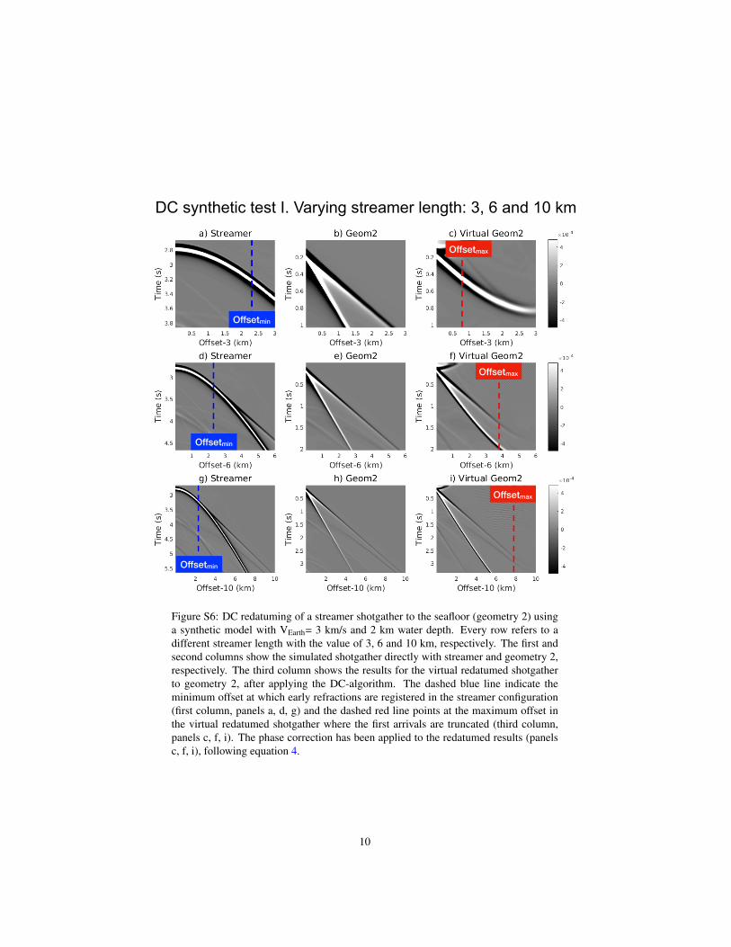
Offsetmin

Offsetmin

Offsetmin

Offsetmax

Offsetmax

Offsetmax

DC synthetic test I. Varying streamer length: 3, 6 and 10 km

Figure S6: DC redatuming of a streamer shotgather to the seafloor (geometry 2) usinga synthetic model with VEarth= 3 km/s and 2 km water depth. Every row refers to adifferent streamer length with the value of 3, 6 and 10 km, respectively. The first andsecond columns show the simulated shotgather directly with streamer and geometry 2,respectively. The third column shows the results for the virtual redatumed shotgatherto geometry 2, after applying the DC-algorithm. The dashed blue line indicate theminimum offset at which early refractions are registered in the streamer configuration(first column, panels a, d, g) and the dashed red line points at the maximum offset inthe virtual redatumed shotgather where the first arrivals are truncated (third column,panels c, f, i). The phase correction has been applied to the redatumed results (panelsc, f, i), following equation 4.

10

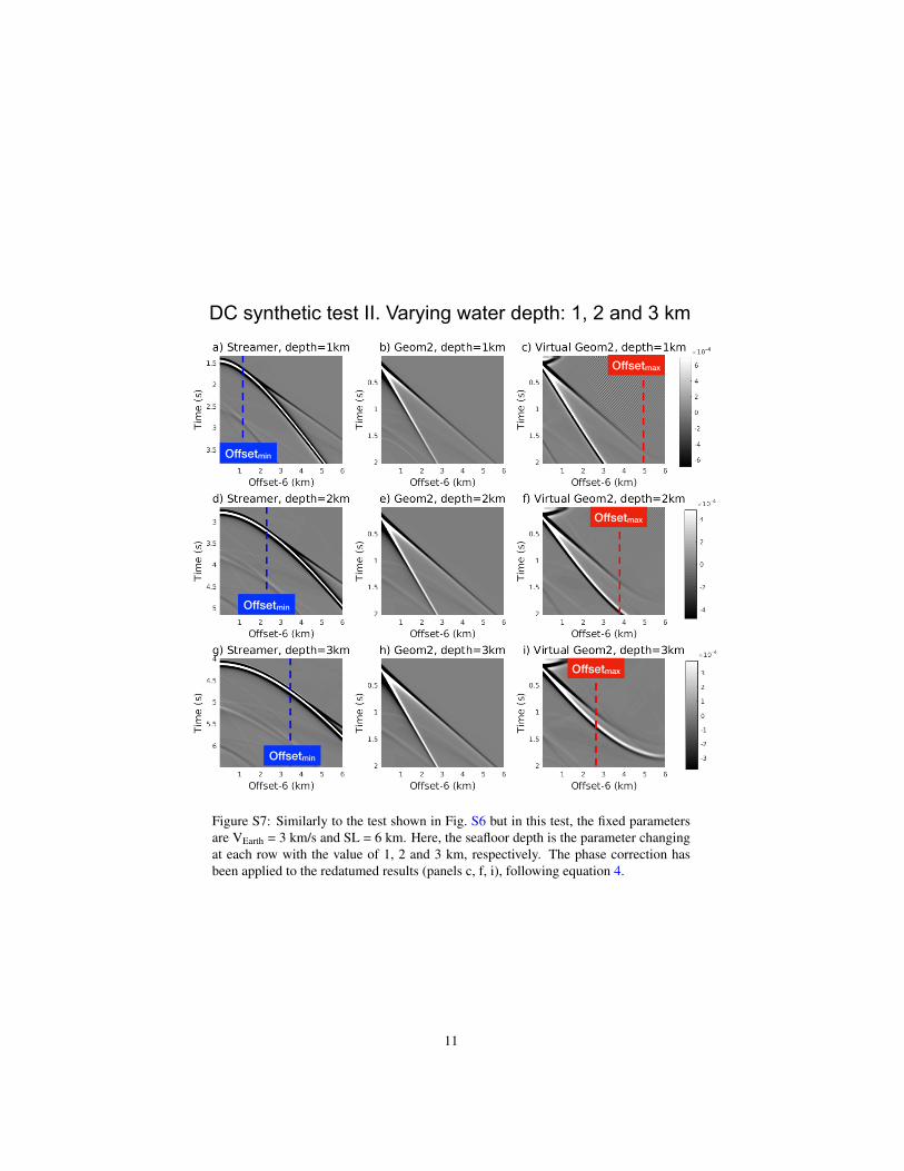
Offsetmin

Offsetmin

Offsetmin

Offsetmax

Offsetmax

Offsetmax

DC synthetic test II. Varying water depth: 1, 2 and 3 km

Figure S7: Similarly to the test shown in Fig. S6 but in this test, the fixed parametersare VEarth = 3 km/s and SL = 6 km. Here, the seafloor depth is the parameter changingat each row with the value of 1, 2 and 3 km, respectively. The phase correction hasbeen applied to the redatumed results (panels c, f, i), following equation 4.

11

Offsetmin

Offsetmin

Offsetmin

Offsetmax

Offsetmax

Offsetmax

DC synthetic test III. Varying VEarth: 2, 3 and 4 km/s

Figure S8: Similarly to the test shown in Fig. S6 and S7 but in this test, the fixedparameters are 2 km/s water depth and SL = 6 km. Here, the subsurface velocity, VEarthis the parameter changing at each row with the value of 2, 3 and 4 km/s respectively.The phase correction has been applied to the redatumed results (panels c, f, i), followingequation 4.

12

Offsetmax

Offsetmax

OffsetminOffsetmin

Offsetmin

Offsetmin2

Offsetmin2 Offsetmin2

Offsetmin2 Offsetmin2

DC synthetic test: benchmark model (2 layers)

Figure S9: Similarly to the test shown in Fig. S6 but in this test, there is a secondsubsurface layer starting at 3 km depth from the sea surface (or 1 km depth from theseafloor) with VEarth = 5 km/s. In this case, the added dotted white lines indicate theminimum offset at which refractions from the second layer of the model are registeredin the streamer. The phase correction has been applied to the redatumed results (panelc2), following equation 4.

13