Constraining models of extended gravity usingGravity Probe B and LARES experiments

S. Capozziello,1,2,3,* G. Lambiase,4,5,† M. Sakellariadou,6,‡ A. Stabile,7,§ and An. Stabile4,5,∥1Dipartimento di Fisica, Università di Napoli “Federico II,”

Complesso Universitario di Monte Sant’Angelo, Edificio G, Via Cinthia, I-80126 Napoli, Italy2Istituto Nazionale di Fisica Nucleare (INFN) Sezione di Napoli,

Complesso Universitario di Monte Sant’Angelo, Edificio G, Via Cinthia, I-80126 Napoli, Italy3Gran Sasso Science Institute (INFN), Viale F. Crispi, 7, I-67100 L’Aquila, Italy

4Dipartimento di Fisica “E.R. Caianiello,” Università degli Studi di Salerno,via G. Paolo II, Stecca 9, I - 84084 Fisciano, Italy

5Istituto Nazionale di Fisica Nucleare (INFN) Sezione di Napoli,Gruppo collegato di Salerno, via G. Paolo II, Stecca 9, I - 84084 Fisciano, Italy

6Department of Physics, King’s College London, University of London,Strand WC2R 2LS London, United Kingdom

7Dipartimento di Ingegneria, Università del Sannio, Palazzo Dell’Aquila Bosco Lucarelli,Corso Garibaldi, 107 - 82100 Benevento, Italy

(Received 30 October 2014; published 9 February 2015)

We consider models of extended gravity and in particular, generic models containing scalar-tensorand higher-order curvature terms, as well as a model derived from noncommutative spectral geometry.Studying, in the weak-field approximation (the Newtonian and post-Newtonian limit of the theory), thegeodesic and Lense-Thirring processions, we impose constraints on the free parameters of such models byusing the recent experimental results of the Gravity Probe B (GPB) and Laser Relativity Satellite (LARES)satellites. The imposed constraint by GPB and LARES is independent of the torsion-balance experiment,though it is much weaker.

DOI: 10.1103/PhysRevD.91.044012 PACS numbers: 04.50.Kd, 04.25.Nx, 04.80.Cc

I. INTRODUCTION

Extended gravity may offer an alternative approachto explain cosmic acceleration and large scale structurewithout considering dark energy and dark matter. In thisframework, while the well-established results of generalrelativity (GR) are retained at intermediate scales, devia-tions at ultraviolet and infrared scales are considered [1]. Insuch models of extended gravity, which may result fromsome effective theory aimed at providing a full quantumgravity formulation, the gravitational interaction may con-tain further contributions, with respect to GR, at galactic,extra-galactic and cosmological scales where, otherwise,large amounts of unknown dark components are required.In the simplest version of extended gravity, the Ricci

curvature scalar R, linear in the Hilbert-Einstein action,could be replaced by a generic function fðRÞ whose trueform could be “reconstructed” by the data. Indeed, in theabsence of a full theory of quantum gravity, one may adoptthe approach that observational data could contribute todefine and constrain the “true” theory of gravity [1–7].

In the weak-field approximation, any relativistic theoryof gravitation yields, in general, corrections to the gravi-tational potentials (e.g., Ref. [8]) which, at the post-Newtonian level and in the parametrized post-Newtonianformalism, could constitute the test bed for these theories[9]. In extended gravity there are further gravitationaldegrees of freedom (related to higher-order terms, non-minimal couplings and scalar fields in the field equations),and moreover the form of the gravitational interaction is nolonger scale invariant. Hence, in a given situation, besidesthe Schwarzschild radius, other characteristic gravitationalscales could come out from dynamics. Such scales, in theweak-field approximation, should exhibit a form of gravi-tational confinement in this way [10]. Considering gravityat intermediate and microscopic scale, the possible viola-tion of the equivalence principle could open the door to testsuch additional degrees of freedom [11].In what follows, we investigate in Sec. II A the weak-

field limit of generic scalar-tensor-higher-order models, inview of constraining their parameters by satellite data likeGravity Probe B and Laser Relativity Satellite (LARES). Inaddition, we consider in Sec. II B a scalar-tensor-higher-order model derived from noncommutative spectralgeometry. The analysis is performed, in Sec. III, in theNewtonian limit, and the solutions are found for a pointlikesource in Sec. III A, and for a rotating balllike source in

*capozziello@na.infn.it†lambiase@sa.infn.it‡mairi.sakellariadou@kcl.ac.uk§arturo.stabile@gmail.com∥anstabile@gmail.com

PHYSICAL REVIEW D 91, 044012 (2015)

1550-7998=2015=91(4)=044012(15) 044012-1 © 2015 American Physical Society

Sec. III B. In Sec. IVA we review the aspects on circularrotation curves and discuss the effects of the parameters ofthe considered models. In Sec. IV B, we analyze all orbitalparameters for the case of a rotating source. The compari-son with the experimental data is performed in Sec. V andour conclusions are drawn in Sec. VI.

II. EXTENDED GRAVITY

We discuss the general case of scalar-tensor-higher-ordergravity where the standard Hilbert-Einstein action isreplaced by a more general action containing a scalar fieldand curvature invariants, like the Ricci scalar R and theRicci tensor Rαβ. We note that the Riemann tensor can bediscarded since the Gauss-Bonnet invariant fixes it in theaction (for details see Ref. [12]). We derive the fieldequations and, in particular, discuss the case of non-commutative geometry in order to show that such anapproach is well founded at the relevant scales.

A. The general case: Scalar-tensor-higher-order gravity

Consider the action

S ¼Z

d4xffiffiffiffiffiffi−g

p ½fðR;RαβRαβ;ϕÞ þ ωðϕÞϕ;αϕ;α þ XLm�;

ð1Þwhere f is an unspecified function of the Ricci scalar R,the curvature invariant RαβRαβ ≐ Y where Rαβ is the Riccitensor, and a scalar field ϕ. Here Lm is the minimallycoupled ordinary matter Lagrangian density, ω is a genericfunction of the scalar field, g is the determinant of metrictensor gμν and

1 X ¼ 8πG. In the metric approach, namelywhen the gravitational field is fully described by the metrictensor gμν only,

2 the field equations are obtained by varyingthe action (1) with respect to gμν, leading to

fRRμν −f þ ωðϕÞϕ;αϕ

;α

2gμν − fR;μν þ gμν□fR

þ 2fYRμαRαν − 2½fYRαðμ�;νÞα þ□½fYRμν�

þ ½fYRαβ�;αβgμν þ ωðϕÞϕ;μϕ;ν ¼ XTμν; ð2Þ

where Tμν ¼ − 1ffiffiffiffi−gp δð ffiffiffiffi−gpLmÞ

δgμν is the energy-momentum ten-

sor of matter, fR ¼ ∂f∂R, fY ¼ ∂f

∂Y and □ ¼ ;σ;σ is the

D’Alembert operator. We use for the Ricci tensor theconvention Rμν ¼ Rσ

μσν, while for the Riemann tensorwe define Rα

βμν ¼ Γαβν;μ þ � � �. The affinity connections

are the usual Christoffel symbols of the metric, namely

Γμαβ ¼ 1

2gμσðgασ;β þ gβσ;α − gαβ;σÞ, and we adopt the signa-

ture ðþ;−;−;−Þ. The trace of the field equation (2) abovereads

fRRþ 2fYRαβRαβ − 2f þ□½3fR þ fYR� þ 2½fYRαβ�;αβ− ωðϕÞϕ;αϕ

;α ¼ XT; ð3Þ

where T ¼ Tσσ is the trace of energy-momentum tensor.

By varying the action (1) with respect to the scalar fieldϕ, we obtain the Klein-Gordon field equation

2ωðϕÞ□ϕþ ωϕðϕÞϕ;αϕ;α − fϕ ¼ 0; ð4Þ

where ωϕ ¼ dωdϕ and fϕ ¼ df

dϕ.In the following subsection we will consider a particular

model derived by a fundamental theory, namely by non-commutative spectral geometry [13,14].

B. The case of noncommutative spectral geometry

Running backwards in time the evolution of ourUniverse, we approach extremely high energy scalesand huge densities within tiny spaces. At such extremeconditions, GR can no longer describe satisfactorily theunderlined physics, and a full quantum gravity theory hasto be invoked. Different quantum gravity approaches havebeen worked out in the literature; they should all lead toGR, considered as an effective theory, as one reachesenergy scales much below the Planck scale.Even though quantum gravity may imply that at Planck

energy scales spacetime is a wildly noncommutativemanifold, one may safely assume that at scales a feworders of magnitude below the Planck scale, the spacetimeis only mildly noncommutative. At such intermediatescales, the algebra of coordinates can be considered asan almost-commutative algebra of matrix valued functions,which if appropriately chosen, can lead to the StandardModel of particle physics. The application of the spectralaction principle [15] to this almost-commutative manifoldled to the noncommutative spectral geometry (NCSG)[16–18], a framework that offers a purely geometricexplanation of the Standard Model of particles coupledto gravity [19,20].For almost-commutative manifolds, the geometry is

described by the tensor product M × F of a four-dimensional compact Riemannian manifold M and adiscrete noncommutative space F , with M describingthe geometry of spacetime and F the internal space ofthe particle physics model. The noncommutative nature ofF is encoded in the spectral triple ðAF ;HF ; DF Þ. ThealgebraAF ¼ C∞ðMÞ of smooth functions onM, playingthe role of the algebra of coordinates, is an involution ofoperators on the finite-dimensional Hilbert space HF ofEuclidean fermions. The operator DF is the Dirac operator∂M ¼ ffiffiffiffiffiffi

−1p

γμ∇sμ on the spin manifold M; it corresponds

1Here we use the convention c ¼ 1.2It is worth noticing that in metric-affine theories, the gravi-

tational field is completely assigned by the metric tensor gμν,while the affinity connections Γα

μν are considered as independentfields [1].

S. CAPOZZIELLO et al. PHYSICAL REVIEW D 91, 044012 (2015)

044012-2

to the inverse of the Euclidean propagator of fermions andis given by the Yukawa coupling matrix and the Kobayashi-Maskawa mixing parameters.The algebra AF has to be chosen so that it can lead to

the Standard Model of particle physics, while it mustalso fulfill noncommutative geometry requirements. It washence chosen to be [21–23]

AF ¼ MaðHÞ ⊕ MkðCÞ;

with k ¼ 2a; H is the algebra of quaternions, which encodesthe noncommutativity of the manifold. The first possiblevalue for k is 2, corresponding to a Hilbert space of fourfermions; it is ruled out from the existence of quarks. Theminimum possible value for k is 4 leading to the correctnumber of k2 ¼ 16 fermions in each of the three generations.Higher values of k can lead to particle physics modelsbeyond the Standard Model [24,25]. The spectral geometryin the product M × F is given by the product rules:

A ¼ C∞ðMÞ ⊕ AF;

H ¼ L2ðM; SÞ ⊕ HF;

D ¼ DM ⊕ 1þ γ5 ⊕ DF; ð5Þ

where L2ðM; SÞ is the Hilbert space of L2 spinors and DMis the Dirac operator of the Levi-Cività spin connection onM. Applying the spectral action principle to the productgeometry M × F leads to the NCSG action

TrðfðDA=ΛÞÞ þ ð1=2ÞhJψ ; Dψi;

split into the bare bosonic action and the fermionic one. Notethat DA ¼ DþAþ ϵ0JAJ−1 are unimodular inner fluctu-ations, f is a cutoff function,Λ fixes the energy scale, J is thereal structure on the spectral triple and ψ is a spinor inthe Hilbert space H of the quarks and leptons. In whatfollows we concentrate on the bosonic part of the action,seen as the bare action at the mass scale Λ which includesthe eigenvalues of the Dirac operator that are smallerthan the cutoff scale Λ, considered as the grand unificationscale. Using heat kernel methods, the trace TrðfðDA=ΛÞ canbe written in terms of the geometrical Seeley–de Wittcoefficients an known for any second-order elliptic differ-ential operator, as Σ∞

n¼0F4−nΛ4−nan where the functionF is defined such that FðD2

AÞ ¼ fðDAÞ. Considering theRiemannian geometry to be four dimensional, the asymp-totic expansion of the trace reads [26,27]

TrðfðDA=ΛÞÞ ∼ 2Λ4f4a0 þ 2Λ2f2a2 þ f0a4 þ � � �þ Λ−2kf−2ka4þ2k þ � � � ; ð6Þ

where fk are the momenta of the smooth even test (cutoff)function which decays fast at infinity, and only enters in themultiplicative factors:

f0 ¼ fð0Þ;

f2 ¼Z

∞

0

fðuÞudu;

f4 ¼Z

∞

0

fðuÞu3du;

f−2k ¼ ð−1Þk k!ð2kÞ! f

ð2kÞð0Þ:

Since the Taylor expansion of the f function vanishesat zero, the asymptotic expansion of the spectral actionreduces to

TrðfðDA=ΛÞÞ ∼ 2Λ4f4a0 þ 2Λ2f2a2 þ f0a4: ð7Þ

Hence, the cutoff function f plays a role only through itsmomenta. f0; f2; f4 are three real parameters, related to thecoupling constants at unification, the gravitational constant,and the cosmological constant, respectively.The NCSG model lives by construction at the grand

unification scale, hence providing a framework to studyearly Universe cosmology [28–31]. The gravitational partof the asymptotic expression for the bosonic sector of theNCSG action,3 including the coupling between the Higgsfield ϕ and the Ricci curvature scalar R, in Lorentziansignature, obtained through a Wick rotation in imaginarytime, reads [19]

SLgrav ¼

Zd4x

ffiffiffiffiffiffi−g

p �R2κ20

þ α0CαβγδCαβγδ

þ τ0R⋆R⋆ − ξ0RjHj2�; ð8Þ

H ¼ ð ffiffiffiffiffiffiffiffiaf0

p=πÞϕ, with a a parameter related to fermion

and lepton masses and lepton mixing. At unification scale(set up by Λ), α0 ¼ −3f0=ð10π2Þ, ξ0 ¼ 1

12.

The square of the Weyl tensor can be expressed in termsof R2 and RαβRαβ as

CαβγδCαβγδ ¼ 2RαβRαβ −2

3R2:

The above action (8) is clearly a particular case of the action(1) describing a general model of an extended theory ofgravity. As we will show in the following, it may lead toeffects observable at local scales (in particular at SolarSystem scales); hence it may be tested against currentgravitational data.

3Note that the obtained action does not suffer from negativeenergy massive graviton modes [32].

CONSTRAINING MODELS OF EXTENDED GRAVITY USING … PHYSICAL REVIEW D 91, 044012 (2015)

044012-3

III. THE WEAK-FIELD LIMIT

We study, in the weak-field approximation, models ofextended gravity at Solar System scales. In order to performthe weak-field limit, we have to perturb Eqs. (2), (3) and (4)in a Minkowski background ημν [33,34].At this point, it is worth discussing briefly some

general issues of the Newtonian and post-Newtonianlimits. In this section, we provide the explicit form ofthe metric tensor needed to compute the approximationsin the field equations for any metric theory of gravity. Ifone considers a system of gravitationally interactingparticles of mass M, the kinetic energy 1

2Mv2 will be,

roughly, of the same order of magnitude as the typicalpotential energy U ¼ GM2=r, with M, r, and v thetypical average values of masses, separations, and veloc-ities, respectively, of these particles. As a consequenceone has v2 ∼ GM

r (for instance, a test particle in a circularorbit of radius r about a central mass M will havevelocity v given in Newtonian mechanics by theexact formula v2 ¼ GM=r). The post-Newtonian

approximation can be described as a method forobtaining the motion of the system to a higher-than-the-first-order approximation (which coincides with theNewtonian mechanics) with respect to the quantitiesGM=r, or v2, assumed to be small with respect to thesquared speed of light. This approximation is some-times also referred to as an expansion in inverse powersof the speed of light.The typical values of the Newtonian gravitational poten-

tial Φ are nowhere larger (in modulus) than 10−5 in theSolar System (in geometrized units Φ is dimensionless).Moreover, planetary velocities satisfy the conditionv2 ≲ −Φ, while the matter pressure p experienced insidethe Sun and the planets is generally smaller than the mattergravitational energy density −ρΦ; in other words4

p=ρ≲ −Φ. As matter of fact, one can consider that thesequantities, as a function of the velocity, give second-ordercontributions as −Φ ∼ v2 ∼Oð2Þ. Then we can set as aperturbative scheme of the metric tensor the followingexpression:

gμν ∼

1þ gð2Þtt ðt;xÞ þ gð4Þtt ðt;xÞ þ… gð3Þti ðt;xÞ þ…

gð3Þti ðt;xÞ þ… −δij þ gð2Þij ðt;xÞ þ…

!¼�1þ 2Φþ 2Ξ 2Ai

2Ai −δij þ 2Ψδij

�;

ϕ ∼ ϕð0Þ þ ϕð2Þ þ… ¼ ϕð0Þ þ φ; ð9Þ

where Φ, Ψ, φ are proportional to the power c−2 (Newtonian limit) while Ai is proportional to c−3 and Ξ to c−4 (post-Newtonian limit). The function f, up to the c−4 order, can be developed as

fðR; RαβRαβ;ϕÞ ¼ fRð0; 0;ϕð0ÞÞRþ fRRð0; 0;ϕð0ÞÞ2

R2 þ fϕϕð0; 0;ϕð0ÞÞ2

ðϕ − ϕð0ÞÞ2

þ fRϕð0; 0;ϕð0ÞÞRϕþ fYð0; 0;ϕð0ÞÞRαβRαβ; ð10Þ

while all other possible contributions in f are negligible [34,36,37]. The field equations (2), (3) and (4) henceread

fRð0; 0;ϕð0ÞÞ�Rtt −

R2

�− fYð0; 0;ϕð0ÞÞ△Rtt −

�fRRð0; 0;ϕð0ÞÞ þ fYð0; 0;ϕð0ÞÞ

2

�△R − fRϕð0; 0;ϕð0ÞÞ△φ ¼ XTtt;

fRð0; 0;ϕð0ÞÞ�Rij þ

R2δij

�− fYð0; 0;ϕð0ÞÞ△Rij þ

�fRRð0; 0;ϕð0ÞÞ þ fYð0; 0;ϕð0ÞÞ

2

�δij△R − fRRð0; 0;ϕð0ÞÞR;ij

− 2fYð0; 0;ϕð0ÞÞRαði;jÞα − fRϕð0; 0;ϕð0ÞÞð∂2

ij − δij△Þφ ¼ XTij;

fRð0; 0;ϕð0ÞÞRti − fYð0; 0;ϕð0ÞÞ△Rti − fRRð0; 0;ϕð0ÞÞR;ti − 2fYð0; 0;ϕð0ÞÞRαðt;iÞα − fRϕð0; 0;ϕð0ÞÞφ;ti

¼ XTti; fRð0; 0;ϕð0ÞÞRþ ½3fRRð0; 0;ϕð0ÞÞ þ 2fYð0; 0;ϕð0ÞÞ�△Rþ 3fRϕð0; 0;ϕð0ÞÞ△φ ¼ −XT;

2ωðϕð0ÞÞ△φþ fϕϕð0; 0;ϕð0ÞÞφþ fRϕð0; 0;ϕð0ÞÞR ¼ 0; ð11Þ

4Typical values of p=ρ are ∼10−5 in the Sun and ∼10−10 in the Earth [35].

S. CAPOZZIELLO et al. PHYSICAL REVIEW D 91, 044012 (2015)

044012-4

where △ is the Laplace operator in the flat space. The geometric quantities Rμν and R are evaluated at the first orderwith respect to the metric potentials Φ, Ψ and Ai. By introducing the quantities5

mR2 ≐ −

fRð0; 0;ϕð0ÞÞ3fRRð0; 0;ϕð0ÞÞ þ 2fYð0; 0;ϕð0ÞÞ ; mY

2 ≐ fRð0; 0;ϕð0ÞÞfYð0; 0;ϕð0ÞÞ ; mϕ

2 ≐ −fϕϕð0; 0;ϕð0ÞÞ

2ωðϕð0ÞÞ ; ð12Þ

and setting fRð0; 0;ϕð0ÞÞ ¼ 1, ωðϕð0ÞÞ ¼ 1=2 for simplicity,6 we get the complete set of differential equations

ð△ −mY2ÞRtt þ

�mY

2

2−mR

2 þ 2mY2

6mR2

△

�RþmY

2fRϕð0; 0;ϕð0ÞÞ△φ

¼ −mY2XTtt; ð△ −mY

2ÞRij þ�mR

2 −mY2

3mR2

∂2ij − δij

�mY

2

2−mR

2 þ 2mY2

6mR2

△

��RþmY

2fRϕð0; 0;ϕð0ÞÞð∂2ij − δij△Þφ

¼ −mY2XTij; ð△ −mY

2ÞRti þmR

2 −mY2

3mR2

R;ti þmY2fRϕð0; 0;ϕð0ÞÞφ;ti

¼ −mY2XTti; ð△ −mR

2ÞR − 3mR2fRϕð0; 0;ϕð0ÞÞ△φ ¼ mR

2XT; ð△ −mϕ2Þφþ fRϕð0; 0;ϕð0ÞÞR ¼ 0:

ð13ÞThe components of the Ricci tensor in Eq. (13) in the weak-field limit read

Rtt ¼1

2△gð2Þtt ¼ △Φ;

Rij ¼1

2gð2Þij;mm −

1

2gð2Þim;mj −

1

2gð2Þjm;mi −

1

2gð2Þtt;ij þ

1

2gð2Þmm;ij ¼ △Ψδij þ ðΨ − ΦÞ;ij;

Rti ¼1

2gð3Þti;mm −

1

2gð2Þim;mt −

1

2gð3Þmt;mi þ

1

2gð2Þmm;ti ¼ △Ai þΨ;ti: ð14Þ

The energy momentum tensor Tμν can be also expanded. For a perfect fluid, when the pressure is negligible withrespect to the mass density ρ, it reads Tμν ¼ ρuμuν with uσuσ ¼ 1. However, the development starts from the zerothorder7; hence Ttt ¼ Tð0Þ

tt ¼ ρ, Tij ¼ Tð0Þij ¼ 0 and Tti ¼ Tð1Þ

ti ¼ ρvi, where ρ is the density mass and vi is the velocityof the source. Thus, Tμν is independent of metric potentials and satisfies the ordinary conservation conditionTμν

;μ ¼ 0. Equations (13) thus read

ð△ −mY2Þ△Φþ

�mY

2

2−mR

2 þ 2mY2

6mR2

△

�RþmY

2fRϕð0; 0;ϕð0ÞÞ△φ ¼ −mY2Xρ; ð15aÞ

�ð△ −mY

2Þ△Ψ −�mY

2

2−mR

2 þ 2mY2

6mR2

△

�R −mY

2fRϕð0; 0;ϕð0ÞÞ△φ

�δij

þ�ð△ −mY

2ÞðΨ − ΦÞ þmR2 −mY

2

3mR2

RþmY2fRϕð0; 0;ϕð0ÞÞφ

�;ij

¼ 0; ð15bÞ�ð△ −mY

2Þ△Ai þmY2Xρvig þ fð△ −mY

2ÞΨþmR2 −mY

2

3mR2

RþmY2fRϕð0; 0;ϕð0ÞÞφ

�;ti¼ 0; ð15cÞ

ð△ −mR2ÞR − 3mR

2fRϕð0; 0;ϕð0ÞÞ△φ ¼ mR2Xρ; ð15dÞ

ð△ −mϕ2Þφþ fRϕð0; 0;ϕð0ÞÞR ¼ 0: ð15eÞ

6We can define a new gravitational constant: X → XfRð0; 0;ϕð0ÞÞ and fRϕð0; 0;ϕ0Þ → fRϕð0; 0;ϕ0ÞfRð0; 0;ϕð0ÞÞ.7This formalism descends from the theoretical setting of Newtonian mechanics which requires the appropriate scheme of

approximation when obtained from a more general relativistic theory. This scheme coincides with a gravity theory analyzed at the firstorder of perturbation in a curved spacetime metric.

5In the Newtonian and post-Newtonian limits, we can consider as a Lagrangian in the action (1), the quantity fðX; YÞ ¼aRþ bR2 þ cRαβRαβ [36]. Then the masses (12) become mR

2 ¼ − a2ð3bþcÞ, mY

2 ¼ ac. For a correct interpretation of these quantities as

real masses, we have to impose a > 0, b < 0 and 0 < c < −3b.

CONSTRAINING MODELS OF EXTENDED GRAVITY USING … PHYSICAL REVIEW D 91, 044012 (2015)

044012-5

In the following we consider the Newtonian and post-Newtonian limits.

A. The Newtonian limit: Solutionsof the fields Φ, φ and R

Equations (15d) and (15e) are a coupled system and, fora pointlike source ρðxÞ ¼ MδðxÞ, admit the solutions

φðxÞ ¼ffiffiffiξ

3

rrgjxj

e−mR~kRjxj − e−mR

~kϕjxj

~k2R − ~k2ϕ;

RðxÞ ¼ −mR2rgjxj

ð~k2R − η2Þe−mR~kRjxj − ð~k2ϕ − η2Þe−mR

~kϕjxj

~k2R − ~k2ϕ;

ð16Þ

where rg is the Schwarzschild radius, ~k2R;ϕ¼1−ξþη2�

ffiffiffiffiffiffiffiffiffiffiffiffiffiffiffiffiffiffiffiffiffiffiffið1−ξþη2Þ2−4η2

p2

, ξ¼3fRϕð0;0;ϕð0ÞÞ2 and η¼mϕ

mR

[37].8 Moreover ξ and η satisfy the conditionðη − 1Þ2 − ξ > 0. The formal solution of the gravitationalpotential Φ, derived from Eq. (15a), reads

ΦðxÞ ¼ −116π2

Zd3x0d3x00

jx − x0je−mY jx0−x″j

jx0 − x00j�4mY

2 −mR2

6Xρðx00Þ

þmY2 −mR

2ð1 − ξÞ6

Rðx00Þ −mR4η2

2ffiffiffi3

p ξ1=2φðx00Þ�;

which for a pointlike source is

ΦðxÞ ¼ −GMjxj�1þ gðξ; ηÞe−mR

~kRjxj

þ�1

3− gðξ; ηÞ

�e−mR

~kϕjxj −4

3e−mY jxj

�; ð17Þ

where

gðξ; ηÞ ¼ 1 − η2 þ ξþffiffiffiffiffiffiffiffiffiffiffiffiffiffiffiffiffiffiffiffiffiffiffiffiffiffiffiffiffiffiffiffiffiffiffiffiffiffiffiffiffiffiffiffiffiffiffiffiffiffiffiffiη4 þ ðξ − 1Þ2 − 2η2ðξþ 1Þ

p6ffiffiffiffiffiffiffiffiffiffiffiffiffiffiffiffiffiffiffiffiffiffiffiffiffiffiffiffiffiffiffiffiffiffiffiffiffiffiffiffiffiffiffiffiffiffiffiffiffiffiffiffiη4 þ ðξ − 1Þ2 − 2η2ðξþ 1Þ

p :

Note that for fY → 0 i.e. mY → ∞, we obtain the sameoutcome for the gravitational potential as in Ref. [37] for anfðR;ϕÞ-theory. The absence of the coupling term betweenthe curvature invariant Y and the scalar field ϕ, as well asthe linearity of the field equations (15), guarantees that thesolution (17) is a linear combination of solutions obtainedwithin an fðR;ϕÞ-theory and an Rþ Y=mY

2-theory.

B. The post-Newtonian limit: Solutionsof the fields Ψ and Ai

Equation (15b) can be formally solved as

ΨðxÞ ¼ ΦðxÞ þmR2 −mY

2

12πmR2

Zd3x0 e

−mY jx−x0j

jx − x0j Rðx0Þ

þmY2ξ1=2

4ffiffiffi3

pπ

Zd3x0 e

−mY jx−x0j

jx − x0j φðx0Þ;

which for a pointlike source reads

ΨðxÞ ¼ −GMjxj�1 − gðξ; ηÞe−mR

~kRjxj

− ½1=3 − gðξ; ηÞ�e−mR~kϕjxj −

2

3e−mY jxj

�; ð18Þ

obtained by setting f…g;ij ¼ 0 in Eq. (15b), while one alsohas f…gδij ¼ 0 leading to

ΨðxÞ¼−1

16π2

Zd3x0d3x00 e−mY jx0−x00j

jx−x0jjx0−x00j

×

�mR

2þ2mY2

6Xρðx00Þ−mY

2−mR2ð1−ξÞ

6Rðx00Þ

þmR4η2

2ffiffiffi3

p ξ1=2φðx00Þ�; ð19Þ

which is however equivalent to solution (18). The solutions(17) and (18) generalize the outcomes of the theoryfðR;RαβRαβÞ [36].From Eq. (15c), we immediately obtain the solution for

Ai, namely

AiðxÞ ¼ −mY

2X16π2

Zd3x0d3x00 e−mY jx0−x00j

jx − x0jjx0 − x00j ρðx00Þv00i :

ð20ÞIn Fourier space, solution (20) presents the massless pole ofgeneral relativity, and the massive one9 is induced by thepresence of the RαβRαβ term. Hence, the solution (20) canbe rewritten as the sum of general relativity contributionsand massive modes. Since we do not consider contributionsinside rotating bodies, we obtain

AiðxÞ¼−X4π

Zd3x0ρðx0Þv0i

jx−x0jþX4π

Zd3x0e

−mY jx−x0j

jx−x0j ρðx0Þv0i:ð21Þ

For a spherically symmetric system (jxj ¼ r) at rest androtating with angular frequency ΩðrÞ, the energy momen-tum tensor Tti is

8The parameter ξ is defined generally as 3fRϕð0;0;ϕð0ÞÞ22fRð0;0;ϕð0ÞÞωðϕð0ÞÞ.

9Note that Eq. (15c) in Fourier space becomesjkj2ðjkj2 þmY

2Þ ~Ai ¼ −mY2X ~Tti and its solution reads

~Ai ¼ −X ~Tti½ 1jkj2 −

1jkj2þm2

Y�.

S. CAPOZZIELLO et al. PHYSICAL REVIEW D 91, 044012 (2015)

044012-6

Tti ¼ ρðxÞvi ¼ TttðrÞ½ΩðrÞ × x�i¼ 3M

4πR3ΘðR − rÞ½ΩðrÞ × x�i; ð22Þ

where R is the radius of the body and Θ is the Heavisidefunction. Since only in general relativity and scalar tensor

theories the Gauss theorem is satisfied, here we have toconsider the potentials Φ, Ψ generated by the ball sourcewith radius R, while they also depend on the shape ofthe source. In fact for any term ∝ e−mr

r , there is a geometricfactor multiplying the Yukawa term, namely FðmRÞ ¼3 mR coshmR−sinhmR

m3R3 . We thus get

ΦballðxÞ ¼ −GMjxj�1þ gðξ; ηÞFðmR

~kRRÞe−mR~kRjxj þ

�1

3− gðξ; ηÞ

�FðmR

~kϕRÞe−mR~kϕjxj −

4FðmYRÞ3

e−mY jxj�;

ΨballðxÞ ¼ −GMjxj�1 − gðξ; ηÞFðmR

~kRRÞe−mR~kRjxj −

�1

3− gðξ; ηÞ

�FðmR

~kϕRÞe−mR~kϕjxj −

2FðmYRÞ3

e−mY jxj�: ð23Þ

For ΩðrÞ ¼ Ω0, the metric potential (21) reads

AðxÞ¼−3MG2πR3

Ω0×Zd3x01−e−mY jx−x0j

jx−x0j ΘðR−r0Þx0: ð24Þ

Making the approximation

e−mY jx−x0j

jx − x0j ∼e−mYr

rþ e−mYrð1þmYrÞ cos α

rr0

rþO

�r02

r2

�;

ð25Þ

where α is the angle between the vectors x, x0, with x ¼ rxwhere x ¼ ðsin θ cosϕ; sin θ sinϕ; cos θÞ and consideringonly the first order of r0=r, we can evaluate the integrationin the vacuum (r > R) as

Zd3x0 e

−mY jx−x0j

jx − x0j ΘðR − r0Þx0 ¼ 4π

15

ð1þmYrÞe−mYrR5

r3x:

ð26Þ

Thus, the field A outside the sphere is

AðxÞ ¼ Gjxj2 ½1 − ð1þmY jxjÞe−mY jxj�x × J; ð27Þ

where J ¼ 2MR2Ω0=5 is the angular momentum of the ball.The modification with respect to general relativity has

the same feature as the one generated by the pointlikesource [38]. From the definition of mR and mY (12), wenote that the presence of a Ricci scalar function[fRRð0Þ ≠ 0] appears only in mR. Considering onlyfðRÞ-gravity (mY → ∞), the solution (27) is unaffectedby the modification in the Hilbert-Einstein action.In the following, we apply the above analysis in the case

of bodies moving in the gravitational field.

IV. THE BODY MOTION IN THE WEAKGRAVITATIONAL FIELD

Let us consider the geodesic equations

d2xμ

ds2þ Γμ

αβ

dxα

dsdxβ

ds¼ 0; ð28Þ

where ds ¼ffiffiffiffiffiffiffiffiffiffiffiffiffiffiffiffiffiffiffiffigαβdxαdxβ

qis the relativistic distance. In

terms of the potentials generated by the ball source withradius R, the components of the metric gμν read

gtt ¼ 1þ2ΦballðxÞ¼ 1−2GMjxj

�1þgðξ;ηÞFðmR

~kRRÞe−mR~kRjxj þ ½1=3−gðξ;ηÞ�FðmR

~kϕRÞe−mR~kϕjxj−

4FðmYRÞ3

e−mY jxj�;

gti ¼ 2AiðxÞ¼2Gjxj2 ½1− ð1þmY jxjÞe−mY jxj�x×J;

gij ¼−δijþ2ΨballðxÞδij ¼−δij−2GMjxj

�1−gðξ;ηÞFðmR

~kRRÞe−mR~kRjxj− ½1=3−gðξ;ηÞ�FðmR

~kϕRÞe−mR~kϕjxj

−2FðmYRÞ

3e−mY jxj

�δij; ð29Þ

and the nonvanishing Christoffel symbols read

Γtti ¼ Γi

tt ¼ ∂iΦball; Γitj ¼

∂iAj − ∂jAi

2; Γi

jk ¼ δjk∂iΨball − δij∂kΨball − δik∂jΨball: ð30ÞLet us consider some specific motions.

CONSTRAINING MODELS OF EXTENDED GRAVITY USING … PHYSICAL REVIEW D 91, 044012 (2015)

044012-7

A. Circular rotation curves in a sphericallysymmetric field

In the Newtonian limit, Eq. (28), neglecting the rotatingcomponent of the source, leads to the usual equation ofmotion of bodies

d2xdt2

¼ −∇ΦballðxÞ; ð31Þ

where the gravitational potential is given by Eq. (23). Thestudy of motion is very simple considering a particularsymmetry for mass distribution ρ; otherwise analyticalsolutions are not available. However, our aim is to evaluatethe corrections to the classical motion in the easiestsituation, namely the circular motion, in which case wedo not consider radial and vertical motions. The conditionof stationary motion on the circular orbit reads

vcðrÞ ¼ffiffiffiffiffiffiffiffiffiffiffiffiffiffiffir∂ΦðrÞ∂r

r; ð32Þ

where vc denotes the velocity.A further remark on Eq. (17) is needed. The structure of

solutions ismathematically similar to the one of fourth-ordergravity fðR;RαβRαβÞ; however there is a fundamentaldifference regarding the algebraic signs of the Yukawacorrections. More precisely, while the Yukawa correctioninduced by a generic function of the Ricci scalar leads to anattractive gravitational force, and the one induced by theRicci tensor squared leads to a repulsive one [39], here theYukawa corrections induced by a generic function of Ricciscalar and a nonminimally coupled scalar field both have apositive coefficient (see for details Ref. [37]). Hence thescalar field gives rise to a stronger attractive force than infðRÞ-gravity, which may imply that fðR;ϕÞ-gravity is abetter choice than fðR;RαβRαβÞ-gravity. However, there is aproblem in the limit jxj → ∞: the interaction is scaledependent (the scalar fields aremassive) and, in the vacuum,the corrections turn off. Thus, at large distances, we recoveronly the classicalNewtonian contribution. In conclusion, the

presence of scalar fields makes the profile smooth, abehavior which is apparent in the study of rotation curves.For an illustration, let us consider the phenomenological

potential ΦSPðrÞ ¼ − GMr ½1þ αe−mSr�, with α and mS free

parameters, chosen by Sanders [40] in an attempt to fitgalactic rotation curves of spiral galaxies in the absence ofdark matter, within the modified Newtonian dynamics(MOND) proposal of Milgrom [41], was further accom-panied by a relativistic partner known as the tensor-vector-scalar (TeVeS) model [42].10 The free parameters selectedby Sanders were α≃ −0.92 and 1=mS ≃ 40 Kpc. Note thatthis potential was recently used for elliptical galaxies [49].In both cases, assuming a negative value for α, an almostconstant profile for rotation curve is recovered; howeverthere are two issues. Firstly, an fðR;ϕÞ-gravity does notlead to that negative value of α, and secondly the presenceof a Yukawa-like correction with negative coefficient leadsto a lower rotation curve and only by resettingG can one fitthe experimental data.Only if we consider a massive, nonminimally coupled

scalar-tensor theory do we get a potential with negativecoefficient in Eq. (17) [37]. In fact setting the gravitational

constant equal to G0 ¼ 2ωðϕð0ÞÞϕð0Þ−42ωðϕð0ÞÞϕð0Þ−3

G∞ϕð0Þ, where G∞ is the

gravitational constant as measured at infinity, and imposingα−1 ¼ 3 − 2ωðϕð0ÞÞϕð0Þ, the potential (17) becomesΦðrÞ ¼ − G∞M

r f1þ αe−ffiffiffiffiffiffiffiffi1−3α

pmϕrg and then the Sanders

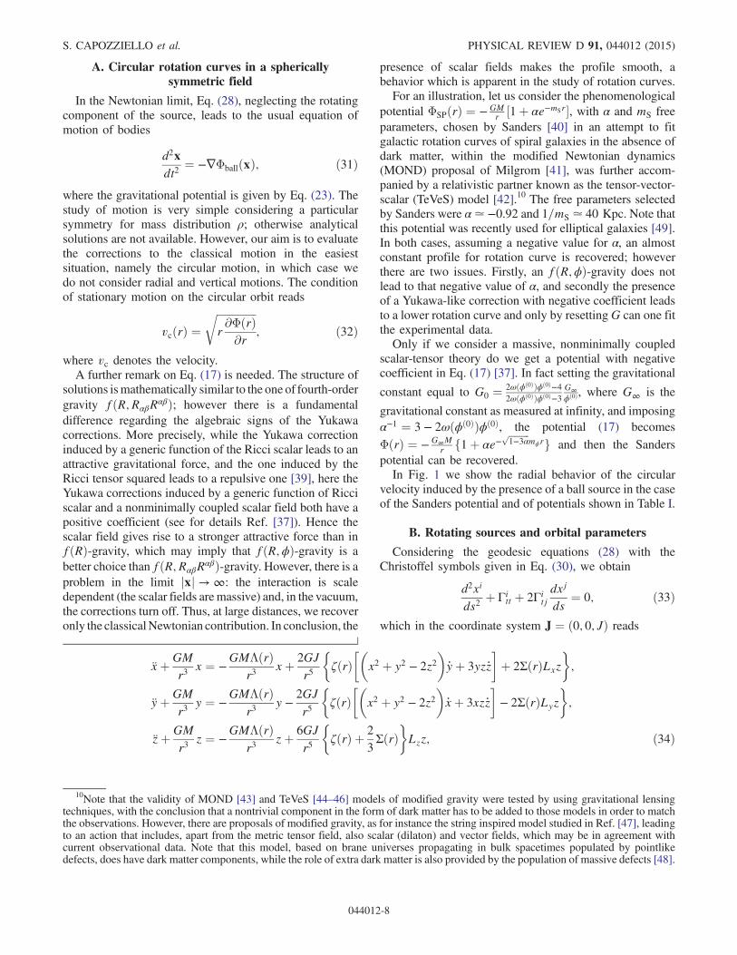
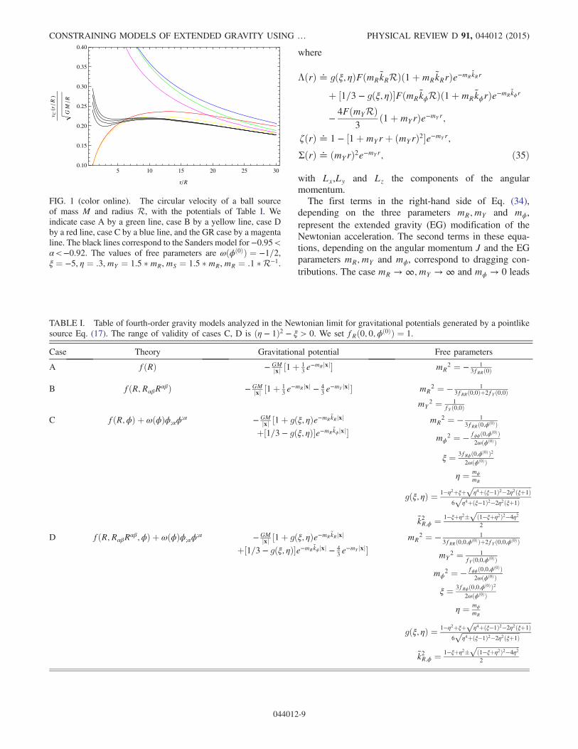
potential can be recovered.In Fig. 1 we show the radial behavior of the circular

velocity induced by the presence of a ball source in the caseof the Sanders potential and of potentials shown in Table I.

B. Rotating sources and orbital parameters

Considering the geodesic equations (28) with theChristoffel symbols given in Eq. (30), we obtain

d2xi

ds2þ Γi

tt þ 2Γitjdxj

ds¼ 0; ð33Þ

which in the coordinate system J ¼ ð0; 0; JÞ reads

xþ GMr3

x ¼ −GMΛðrÞ

r3xþ 2GJ

r5

�ζðrÞ

��x2 þ y2 − 2z2

�_yþ 3yz_z

�þ 2ΣðrÞLxz

�;

yþ GMr3

y ¼ −GMΛðrÞ

r3y −

2GJr5

�ζðrÞ

��x2 þ y2 − 2z2

�_xþ 3xz_z

�− 2ΣðrÞLyz

�;

zþ GMr3

z ¼ −GMΛðrÞ

r3zþ 6GJ

r5

�ζðrÞ þ 2

3ΣðrÞ

�Lzz; ð34Þ

10Note that the validity of MOND [43] and TeVeS [44–46] models of modified gravity were tested by using gravitational lensingtechniques, with the conclusion that a nontrivial component in the form of dark matter has to be added to those models in order to matchthe observations. However, there are proposals of modified gravity, as for instance the string inspired model studied in Ref. [47], leadingto an action that includes, apart from the metric tensor field, also scalar (dilaton) and vector fields, which may be in agreement withcurrent observational data. Note that this model, based on brane universes propagating in bulk spacetimes populated by pointlikedefects, does have dark matter components, while the role of extra dark matter is also provided by the population of massive defects [48].

S. CAPOZZIELLO et al. PHYSICAL REVIEW D 91, 044012 (2015)

044012-8

where

ΛðrÞ ≐ gðξ; ηÞFðmR~kRRÞð1þmR

~kRrÞe−mR~kRr

þ ½1=3 − gðξ; ηÞ�FðmR~kϕRÞð1þmR

~kϕrÞe−mR~kϕr

−4FðmYRÞ

3ð1þmYrÞe−mYr;

ζðrÞ ≐ 1 − ½1þmYrþ ðmYrÞ2�e−mYr;

ΣðrÞ ≐ ðmYrÞ2e−mYr; ð35Þ

with Lx,Ly and Lz the components of the angularmomentum.The first terms in the right-hand side of Eq. (34),

depending on the three parameters mR;mY and mϕ,represent the extended gravity (EG) modification of theNewtonian acceleration. The second terms in these equa-tions, depending on the angular momentum J and the EGparameters mR;mY and mϕ, correspond to dragging con-tributions. The case mR → ∞; mY → ∞ and mϕ → 0 leads

TABLE I. Table of fourth-order gravity models analyzed in the Newtonian limit for gravitational potentials generated by a pointlikesource Eq. (17). The range of validity of cases C, D is ðη − 1Þ2 − ξ > 0. We set fRð0; 0;ϕð0ÞÞ ¼ 1.

Case Theory Gravitational potential Free parameters

A fðRÞ − GMjxj ½1þ 1

3e−mRjxj� mR

2 ¼ − 13fRRð0Þ

B fðR; RαβRαβÞ − GMjxj ½1þ 1

3e−mRjxj − 4

3e−mY jxj� mR

2 ¼ − 13fRRð0;0Þþ2fY ð0;0Þ

mY2 ¼ 1

fY ð0;0ÞC fðR;ϕÞ þ ωðϕÞϕ;αϕ

;α − GMjxj ½1þ gðξ; ηÞe−mR

~kRjxj

þ½1=3 − gðξ; ηÞ�e−mR~kϕjxj�

mR2 ¼ − 1

3fRRð0;ϕð0ÞÞ

mϕ2 ¼ − fϕϕð0;ϕð0ÞÞ

2ωðϕð0ÞÞ

ξ ¼ 3fRϕð0;ϕð0ÞÞ22ωðϕð0ÞÞ

η ¼ mϕ

mR

gðξ; ηÞ ¼ 1−η2þξþffiffiffiffiffiffiffiffiffiffiffiffiffiffiffiffiffiffiffiffiffiffiffiffiffiffiffiffiffiffiffiη4þðξ−1Þ2−2η2ðξþ1Þ

p6ffiffiffiffiffiffiffiffiffiffiffiffiffiffiffiffiffiffiffiffiffiffiffiffiffiffiffiffiffiffiffiη4þðξ−1Þ2−2η2ðξþ1Þ

p

~k2R;ϕ ¼ 1−ξþη2�ffiffiffiffiffiffiffiffiffiffiffiffiffiffiffiffiffiffiffiffiffiffiffið1−ξþη2Þ2−4η2

p2

D fðR; RαβRαβ;ϕÞ þ ωðϕÞϕ;αϕ;α − GM

jxj ½1þ gðξ; ηÞe−mR~kRjxj

þ½1=3 − gðξ; ηÞ�e−mR~kϕ jxj − 4

3e−mY jxj�

mR2 ¼ − 1

3fRRð0;0;ϕð0ÞÞþ2fY ð0;0;ϕð0ÞÞ

mY2 ¼ 1

fY ð0;0;ϕð0ÞÞ

mϕ2 ¼ − fϕϕð0;0;ϕð0ÞÞ

2ωðϕð0ÞÞ

ξ ¼ 3fRϕð0;0;ϕð0ÞÞ22ωðϕð0ÞÞ

η ¼ mϕ

mR

gðξ; ηÞ ¼ 1−η2þξþffiffiffiffiffiffiffiffiffiffiffiffiffiffiffiffiffiffiffiffiffiffiffiffiffiffiffiffiffiffiffiη4þðξ−1Þ2−2η2ðξþ1Þ

p6ffiffiffiffiffiffiffiffiffiffiffiffiffiffiffiffiffiffiffiffiffiffiffiffiffiffiffiffiffiffiffiη4þðξ−1Þ2−2η2ðξþ1Þ

p

~k2R;ϕ ¼ 1−ξþη2�ffiffiffiffiffiffiffiffiffiffiffiffiffiffiffiffiffiffiffiffiffiffiffið1−ξþη2Þ2−4η2

p2

5 10 15 20 25 300.10

0.15

0.20

0.25

0.30

0.35

0.40

r R

v Cr

R

GM

R

FIG. 1 (color online). The circular velocity of a ball sourceof mass M and radius R, with the potentials of Table I. Weindicate case A by a green line, case B by a yellow line, case Dby a red line, case C by a blue line, and the GR case by a magentaline. The black lines correspond to the Sanders model for −0.95<α<−0.92. The values of free parameters are ωðϕð0ÞÞ ¼ −1=2,ξ ¼ −5, η ¼ :3,mY ¼ 1.5 �mR,mS ¼ 1.5 �mR,mR ¼ :1 �R−1.

CONSTRAINING MODELS OF EXTENDED GRAVITY USING … PHYSICAL REVIEW D 91, 044012 (2015)

044012-9

to ΛðrÞ → 0, ζðrÞ → 1 and ΣðrÞ → 0, and hence onerecovers the familiar results of GR [50]. These additionalgravitational terms can be considered as perturbations ofNewtonian gravity, and their effects on planetary motionscan be calculated within the usual perturbative schemesassuming the Gauss equations [51]. We will follow thisapproach in what follows.Let us consider the right-hand side of Eq. (34) as the

components ðAx; Ay; AzÞ of the perturbing acceleration inthe system (X; Y; Z) (see Fig. 2), with X the axis passingthrough the vernal equinox γ, Y the transversal axis, and Zthe orthogonal axis parallel to the angular momentum J ofthe central body. In the system (S; T;W), the threecomponents can be expressed as ðAs; At; AwÞ, with S theradial axis, T the transversal axis, and W the orthogonalone. Wewill adopt the standard notation: a is the semimajoraxis; e is the eccentricity; p ¼ að1 − e2Þ is the semilatusrectum; i is the inclination; Ω is the longitude of theascending node N; ~ω is the longitude of the pericenter Π;M0 is the longitude of the satellite at time t ¼ 0; ν is the trueanomaly; u is the argument of the latitude given byu ¼ νþ ~ω −Ω; n is the mean daily motion equal ton ¼ ðGM=a3Þ1=2; and C is twice the velocity,namely C ¼ r2 _νa2ð1 − e2Þ1=2.The transformation rules between the coordinates frames

(X; Y; Z) and (S; T;W) are

x ¼ rðcos u cosΩ − sin u sinΩ cos iÞ;y ¼ rðcos u sinΩþ sin u cosΩ cos iÞ;z ¼ r sin u sin i

r ¼ p1þ e cos ν

; ð36Þ

and the components of the angular momentum obey theequations

Lx ¼ y_z − z_y ¼ C sin i sinΩ;

Ly ¼ z_x − x_z ¼ −C cosΩ sin i;

Lz ¼ x_y − y_x ¼ C cos i: ð37Þ

The components of the perturbing acceleration in the(S; T;W) system read

As ¼ −GMΛðrÞ

r2þ 2GJC cos i

r4ζðrÞ;

At ¼ −2GJCe cos i sin ν

pr3ζðrÞ;

Aw ¼ 2GJC sin ir4

��re sin ν cos u

pþ 2 sin u

�ζðrÞ

þ 2 sin uΣðrÞ�: ð38Þ

The As component has two contributions: the former oneresults from the modified Newtonian potential ΦballðxÞ,while the latter one results from the gravitomagnetic fieldAi and it is a higher order term than the first one. Notethat the components At and Aw depend only on thegravitomagnetic field. The Gauss equations for the varia-tions of the six orbital parameters, resulting from theperturbing acceleration with components Ax; Ay; Az, read

dadt

¼ _aEG ¼ 2eGMΛðrÞ sin νnffiffiffiffiffiffiffiffiffiffiffiffiffi1 − e2

pC

_ν;

dedt

¼ _eGR þ _eEG ¼ffiffiffiffiffiffiffiffiffiffiffiffiffi1 − e2

pGMΛðrÞ sin νnaC

_νþ _eGR½1 − e−mYrð1þmYrþ ðmYrÞ2Þ�;dΩdt

¼ _ΩGR þ _ΩEG ¼ _ΩGRf1 − e−mYr½1þmYrþ ð1þ fðν; u; eÞÞðmYrÞ2�g;didt

¼ _iGR þ _iEG ¼ _iGRf1 − e−mYr½1þmYrþ ð1þ fðν; u; eÞÞðmYrÞ2�g;

d ~ωdt

¼ _~ωGR þ _~ωEG ¼ −ffiffiffiffiffiffiffiffiffiffiffiffiffi1 − e2

pGMΛðrÞ cos νnaeC

_νþ _~ωGR½1 − e−mYrð1þmYrþ ðmYrÞ2Þ� − 2sin2i2_ΩGRfðν; u; eÞΣðrÞ;

dM0

dt¼ _M0

GR þ _M0EG ¼ −

GMΛðrÞnaC

�2raþ e

ffiffiffiffiffiffiffiffiffiffiffiffiffi1 − e2

p

1þffiffiffiffiffiffiffiffiffiffiffiffiffi1 − e2

p cos ν

�_νþ _M0

GR½1 − e−mYrð1þmYrþ ðmYrÞ2Þ�

− 2sin2i2_ΩGRfðν; u; eÞΣðrÞ; ð39Þ

S. CAPOZZIELLO et al. PHYSICAL REVIEW D 91, 044012 (2015)

044012-10

where

_eGR¼2GJcosisinν

aC_ν;

_ΩGR¼2GJsinu

pC½esinνcosuþ2ð1þecosνÞsinu�_ν;

_iGR¼2GJcosusini

Cp½esinνcosuþ2ð1þecosνÞsinu�_ν;

_~ωGR¼−2GJcosi

aC

�2þ1þe2

ecosν

�_νþ2sin2

i2_ΩGR;

_M0GR¼−

4GJcosina2p

ð1þecosνÞ_νþ e2

1þffiffiffiffiffiffiffiffiffiffiffi1−e2

p _~ωGR

þ2ffiffiffiffiffiffiffiffiffiffiffi1−e2

psin2

i2_ΩGR;

fðν;u;eÞ¼ 1þecosν

1þeðsinνcotu2

þcosνÞ : ð40Þ

Hence, we have derived the corresponding equations of thesix orbital parameters for extended gravity, with thedynamics of a; e; ~ω; L0 depending mainly on the termsrelated to the modifications of the Newtonian potential,while the dynamics of Ω and i depend only on the draggingterms.Considering an almost circular orbit (e ≪ 1), we inte-

grate the Gauss equations with respect to the only anomalyν, from 0 to νðtÞ ¼ nt, since all other parameters have a

slower evolution than ν; hence they can be considered asconstraints with respect to ν. At first order we get

ΔaðtÞ¼0;

ΔeðtÞ¼0;

ΔiðtÞ¼GJe2 sinina3

e−mYpðmYpÞ2�1þðmYpÞ2

2ðmYp−4Þ

�×sinð ~ωðtÞ−ΩðtÞÞνðtÞþOðe4Þ;

ΔΩðtÞ¼2GJna3

½1−e−mYpð1þmYpþ2ðmYpÞ2Þ�νðtÞþOðe2Þ;

Δ ~ωðtÞ¼� ~ΛðpÞ

2−2GJna3

½3cosi−1

þe−mYpð1þmYpþ3

2ðmYpÞ2

−ð3þ3mYpþ3ðmYpÞ2

þ 1

12ðmYpÞ3ÞcosiÞ�

�νðtÞþOðe2Þ;

ΔM0ðtÞ¼�2ΛðpÞ−2GJ

na3½3cosi−1

−e−mYpð1þmYpþ2ðmYpÞ2Þðcosi−1Þ��νðtÞ

þOðe2Þ; ð41Þ

where

~ΛðpÞ ≐ gðξ; ηÞFðmR~kRRÞðmR

~kRpÞ2e−mR~kRp

þ ½1=3 − gðξ; ηÞ�FðmR~kϕRÞðmR

~kϕpÞ2e−mR~kϕp

−4FðmYRÞ

3ðmYpÞ2e−mYp: ð42Þ

We hence notice that the contributions to the semimajoraxis a and eccentricity e vanish, as in GR, while thereare nonzero contributions to i, Ω, ~ω and M0. In particular,the contributions to the inclination i and the longitude ofthe ascending nodeΩ depend only on the drag effects of therotating central body, while the contributions to the peri-center longitude ~ω and mean longitude at M0 depend alsoon the modified Newtonian potential. Finally, note that inthe extended gravity model we have considered here, theinclination i has a nonzero contribution, in contrast to theresult obtained within GR, and also Δ ~ωðtÞ ≠ ΔM0ðtÞ,given by

FIG. 2 (color online). i ¼ ∢ YNΠ is the inclination; Ω ¼ ∢XON is the longitude of the ascending node N; ~ω ¼ broken∢XOΠ is the longitude of the pericenter Π; ν ¼ ∢ ΠOP is the trueanomaly; u ¼ ∢ ΩOP ¼ νþ ~ω − Ω is the argument of thelatitude; J is the angular momentum of rotation of the centralbody; and JSatellite is the angular momentum of revolution of asatellite around the central body.

CONSTRAINING MODELS OF EXTENDED GRAVITY USING … PHYSICAL REVIEW D 91, 044012 (2015)

044012-11

Δ ~ωðtÞ−ΔM0ðtÞ≃� ~ΛðpÞ− 4ΛðpÞ

2þ 2GJ

na3e−mYp

�ðmYpÞ22

þ�2þ 2mYpþðmYpÞ2

þðmYpÞ312

�cos i

��νðtÞþOðe2Þ:

ð43ÞIn the limit mR → ∞; mY → ∞ and mϕ → 0, we obtain thewell-known results of GR.In the following section, we use recent experimental

results obtained from the Gravity Probe B and LARESsatellites in order to constrain the free parameter mY whichappears in the context of a specific model of extendedgravity derived from a fundamental theory, namely non-commutative geometry. More precisely, we constrain thefree parameter by demanding the deviation from the GRresult be within the accuracy of the measured effect.

V. EXPERIMENTAL CONSTRAINTS

The orbiting gyroscope precession can be split into apart generated by the metric potentials, Φ and Ψ, and onegenerated by the vector potentialA. The equation of motionfor the gyrospin three-vector S is

dSdt

¼ dSdt

Gþ dS

dt

LT

ð44Þ

where the geodesic and Lense-Thirring precessions are

dSdt

G¼ ΩG × S with ΩG ¼ ∇ðΦþ 2ΨÞ

2× v;

dSdt

LT

¼ ΩLT × S with ΩLT ¼ ∇ ×A2

: ð45Þ

The geodesic precession, ΩG, can be written as the sumof two terms, one obtained with GR and the other being theextended gravity contribution. Then we have

ΩG ¼ ΩðGRÞG þ ΩðEGÞ

G ; ð46Þ

where

ΩðGRÞG ¼ 3GM

2jxj3 x × v;

ΩðEGÞG ¼ −

�gðξ; ηÞðmR

~kRrþ 1ÞFðmR~kRRÞe−mR

~kRr þ 8

3ðmYrþ 1ÞFðmYRÞe−mYr

þ�1

3− gðξ; ηÞ

�ðmR

~kϕrþ 1ÞFðmR~kϕRÞe−mR

~kϕr

�ΩðGRÞ

G

3; ð47Þ

where jxj ¼ r. Similarly one has

ΩLT ¼ ΩðGRÞLT þΩðEGÞ

LT ; ð48Þ

with

ΩðGRÞLT ¼ G

2r3J;

ΩðEGÞLT ¼ −e−mYrð1þmYrþmY

2r2ÞΩðGRÞLT ;

ð49Þ

where we have assumed that, on the average, hðJ · xÞxi ¼ 0.

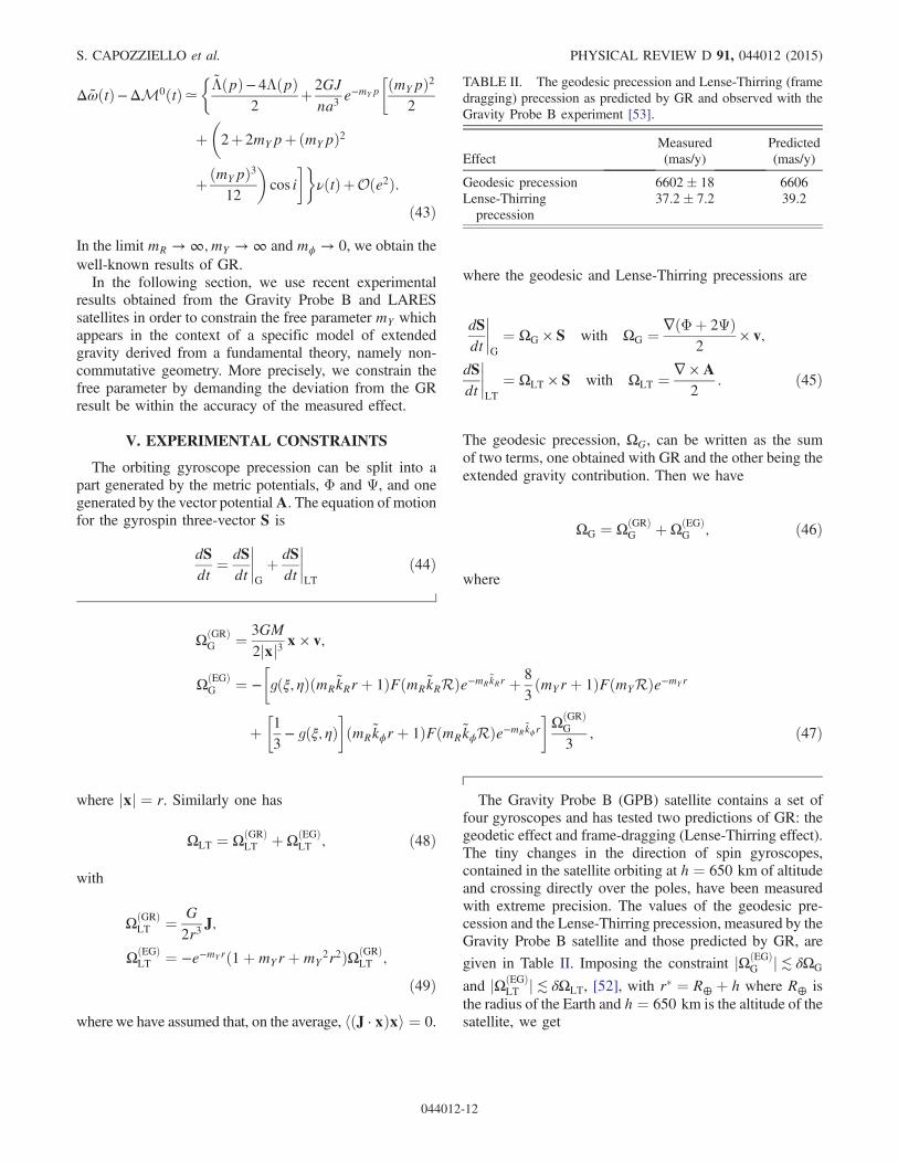
The Gravity Probe B (GPB) satellite contains a set offour gyroscopes and has tested two predictions of GR: thegeodetic effect and frame-dragging (Lense-Thirring effect).The tiny changes in the direction of spin gyroscopes,contained in the satellite orbiting at h ¼ 650 km of altitudeand crossing directly over the poles, have been measuredwith extreme precision. The values of the geodesic pre-cession and the Lense-Thirring precession, measured by theGravity Probe B satellite and those predicted by GR, are

given in Table II. Imposing the constraint jΩðEGÞG j≲ δΩG

and jΩðEGÞLT j≲ δΩLT, [52], with r� ¼ R⊕ þ h where R⊕ is

the radius of the Earth and h ¼ 650 km is the altitude of thesatellite, we get

TABLE II. The geodesic precession and Lense-Thirring (framedragging) precession as predicted by GR and observed with theGravity Probe B experiment [53].

EffectMeasured(mas/y)

Predicted(mas/y)

Geodesic precession 6602� 18 6606Lense-Thirringprecession

37.2� 7.2 39.2

S. CAPOZZIELLO et al. PHYSICAL REVIEW D 91, 044012 (2015)

044012-12

gðξ; ηÞðmR~kRr� þ 1ÞFðmR

~kRR⊕Þe−mR~kRr� þ ½1=3 − gðξ; ηÞ�ðmR

~kϕr� þ 1ÞFðmR~kϕR⊕Þe−mR

~kϕr�

þ 8

3ðmYr� þ 1ÞFðmYR⊕Þe−mYr� ≲ 3δjΩGj

jΩðGRÞG j

≃ 0.008;

ð1þmYr� þmY2r�2Þe−mYr� ≲ δjΩLTj

jΩðGRÞLT j

≃ 0.19; ð50Þ

since, from the experiments, we have jΩðGRÞG j ¼ 6606 mas

and δjΩGj ¼ 18 mas, jΩðGRÞLT j ¼ 37.2 mas and δjΩLTj ¼

7.2 mas. From Eq. (50) we thus obtain that mY ≥7.3 × 10−7m−1.The Laser Relativity Satellite (LARES) mission [54] of

the Italian Space Agency is designed to test the frame-dragging and the Lense-Thirring effect, to within 1% ofthe value predicted in the framework of GR. The body ofthis satellite has a diameter of about 36.4 cm and weightsabout 400 kg. It was inserted in an orbit with 1450 km ofperigee, an inclination of 69.5� 1 degrees and eccentricity9.54 × 10−4. It allows us to obtain a stronger constraintfor mY :

ð1þmYr� þmY2r�2Þe−mYr� ≲ δjΩLTj

jΩðGRÞLT j

≃ 0.01; ð51Þ

from the which we obtain mY ≥ 1.2 × 10−6m−1.In the specific case of the noncommutative spectral

geometry model, the quantities (12) become mR → ∞,

mY ¼ffiffiffiffiffiffiffiffiffiffiffiffiffiffiffiffiffiffiffiffiffi5π2ðk2

0Hð0Þ−6Þ

36f0k20

randmϕ¼0, implying that ξ ¼ af0ðHð0ÞÞ2

12π2,

η ¼ 0, gðξ; ηÞ ¼ af0ðHð0ÞÞ2þ12π2

6jaf0ðHð0ÞÞ2−12π2j þ 16

and ~k2R;ϕ ¼1 − af0ðHð0ÞÞ2

12π2; 0. The first relation (50) becomes

8

3ðmYr� þ 1ÞFðmYR⊕Þe−mYr� ≲ 0.008;

hence the constraint on mY imposed from GPB is

mY > 7.1 × 10−5 m−1;

whereas the LARES experiment (51) implies

mY > 1.2 × 10−6 m−1;

a bound similar to the one obtained earlier on using binarypulsars [55], or the Gravity Probe B data [52].However, a more stringent constraint has been obtained

using torsion balance experiments. More precisely, as it hasbeen shown in Ref. [52], using results from laboratoryexperiments designed to test the fifth force, one arrives tothe tightest constraint mY > 104 m−1.

In conclusion, using data from the Gravity Probe B andLARES missions, we obtain similar constraints on mY , aresult that one could have anticipated since both experi-ments are designed to test the same type of physicalphenomenon. However, by using the stronger constraintfor mY, namely mY > 104 m−1, we observe that themodifications to the orbital parameters (39) induced bynoncommutative spectral geometry are indeed small, con-firming the consistency between the predictions of NCSGas a gravitational theory beyond GR and the Gravity ProbeB and LARES measurements. At this point let us stressthat, in principle, space-based experiments can be used totest parameters of fundamental theories.

VI. CONCLUSIONS

In the context of extended gravity, we have studied thelinearized field equations in the limit of weak gravitationalfields and small velocities generated by rotating gravita-tional sources, aimed at constraining the free parameters,which can be seen as effective masses (or lengths), usingrecent recent experimental results. We have studied theprecession of spin of a gyroscope orbiting about a rotatinggravitational source. Such a gravitational field gives rise,according to GR predictions, to geodesic and Lense-Thirring processions, the latter being strictly related tothe off-diagonal terms of the metric tensor generated by therotation of the source. We have focused in particular on thegravitational field generated by the Earth, and on the recentexperimental results obtained by the Gravity Probe Bsatellite, which tested the geodesic and Lense-Thirringspin precessions with high precision.In particular, we have calculated the corrections of the

precession induced by scalar, tensor and curvature correc-tions. Considering an almost circular orbit, we integratedthe Gauss equations and obtained the variation of theparameters at first order with respect to the eccentricity. Wehave shown that the induced EG effects depend on theeffective massesmR,mY andmϕ (41), while the nonvalidityof the Gauss theorem implies that these effects also dependon the geometric form and size of the rotating source.Requiring that the corrections be within the experimentalerrors, we then imposed constraints on the free parametersof the considered EG model. Merging the experimentalresults of Gravity Probe B and LARES, our results can besummarized as follows:

CONSTRAINING MODELS OF EXTENDED GRAVITY USING … PHYSICAL REVIEW D 91, 044012 (2015)

044012-13

gðξ; ηÞðmR~kRr� þ 1ÞFðmR

~kRR⊕Þe−mR~kRr�

þ ½1=3 − gðξ; ηÞ�ðmR~kϕr� þ 1ÞFðmR

~kϕR⊕Þe−mR~kϕr�

þ 8

3ðmYr� þ 1ÞFðmYR⊕Þe−mYr� ≲ 0.008; ð52Þ

and

mY ≥ 1.2 × 10−6m−1: ð53Þ

It is interesting to note that the field equation for thepotential Ai, Eq. (15c), is time independent provided thepotential Φ is time independent. This aspect guaranteesthat the solution Eq. (27) does not depend on the massesmR andmϕ and, in the case of fðR;ϕÞ gravity, the solution

is the same as in GR. In the case of spherical symmetry,the hypothesis of a radially static source is no longerconsidered, and the obtained solutions depend on thechoice of fðR;ϕÞ ET model, since the geometric factorFðxÞ is time dependent. Hence in this case, gravitomag-netic corrections to GR emerge with time-dependentsources.The case of noncommutative spectral geometry that

we discussed above deserves a final remark. This modeldescends from a fundamental theory and can be consi-dered as a particular case of extended gravity. Its param-eters can be probed in the weak-field limit and at localscales, opening new perspectives worthy of furtherdevelopment [11,56].

[1] S. Capozziello and M. De Laurentis, Phys. Rep. 509, 167(2011).

[2] S. Nojiri and S. D. Odintsov, Phys. Rep. 505, 59(2011).

[3] S. Nojiri and S. D. Odintsov, Int. J. Geom. Methods Mod.Phys. 04, 115 (2007).

[4] S. Capozziello and M. Francaviglia, Gen. Relativ. Gravit.40, 357 (2008).

[5] S. Capozziello, M. De Laurentis, and V. Faraoni, OpenAstron. J. 2, 1874 (2009).

[6] S. Capozziello and V. Faraoni, Beyond Einstein Gravity: ASurvey of Gravitational Theories for Cosmology andAstrophysics, Fundamental Theories of Physics Vol. 170(Springer, New York, 2010).

[7] S. Capozziello and M. De Laurentis, Invariance Principlesand Extended Gravity: Theory and Probes (Nova SciencePublishers, New York, 2010).

[8] I. Quandt and H. J. Schmidt, Astron. Nachr. 312, 97(1991); P. Teyssandier, Classical Quantum Gravity 6,219 (1989); S. Capozziello and G. Lambiase, Int. J.Mod. Phys. D 12, 843 (2003); S. Calchi Novati, S.Capozziello, and G. Lambiase, Gravitation Cosmol. 6,173 (2000).

[9] C. M. Will, Theory and Experiment in GravitationalPhysics, 2nd ed. (Cambridge University Press, Cambridge,UK, 1993).

[10] S. Capozziello and M. De Laurentis, Ann. Phys. (Berlin)524, 545 (2012).

[11] B. Altschul, Q. G. Bailey et al., Adv. Space Res. (to bepublished).

[12] S. Capozziello and A. Stabile, Classical Quantum Gravity26, 085019 (2009).

[13] A. Connes, Noncommutative Geometry (Academic Press,New York, 1994).

[14] A. Connes and M. Marcolli, Noncommutative Geometry,Quantum Fields and Motives (Hindustan Book Agency,India, 2008).

[15] A. H. Chamseddine and A. Connes, Commun. Math. Phys.186, 731 (1997).

[16] M. Sakellariadou, Int. J. Mod. Phys. D 20, 785 (2011).[17] M. Sakellariadou, Proc. Sci., CORFU (2011) 053

[arXiv:1204.5772].[18] K. van den Dungen and W. D. van Suijlekom, Rev. Math.

Phys. 24, 1230004 (2012).[19] A. H. Chamseddine, A. Connes, and M. Marcolli, Adv.

Theor. Math. Phys. 11, 991 (2007).[20] A. H. Chamseddine and A. Connes, J. High Energy Phys. 09

(2012) 104.[21] A. H. Chamseddine and A. Connes, Phys. Rev. Lett. 99,

191601 (2007).[22] M. Sakellariadou, A. Stabile, and G. Vitiello, Phys. Rev. D

84, 045026 (2011).[23] M. V. Gargiulo, M. Sakellariadou, and G. Vitiello, Eur.

Phys. J. C 74, 2695 (2014).[24] A. Devastato, F. Lizzi, and P. Martinetti, J. High Energy

Phys. 01 (2014) 042.[25] A. H. Chamseddine, A. Connes, and W. D. van Suijlekom,

J. High Energy Phys. 11 (2013) 132.[26] A. H. Chamseddine and A. Connes, J. Math. Phys. (N.Y.)

47, 063504 (2006).[27] A. H. Chamseddine and A. Connes, Commun. Math. Phys.

293, 867 (2010).[28] W. Nelson and M. Sakellariadou, Phys. Rev. D 81, 085038

(2010).[29] W. Nelson and M. Sakellariadou, Phys. Lett. B 680, 263

(2009).[30] M. Marcolli and E. Pierpaoli, Adv. Theor. Math. Phys. 14

691 (2010).[31] M. Buck, M. Fairbairn, and M. Sakellariadou, Phys. Rev. D

82, 043509 (2010).[32] J. F. Donoghue, Phys. Rev. D 50, 3874 (1994).[33] S. Capozziello, A. Stabile, and A. Troisi, Phys. Rev. D 76,

104019 (2007).[34] A. Stabile, Phys. Rev. D 82, 064021 (2010).

S. CAPOZZIELLO et al. PHYSICAL REVIEW D 91, 044012 (2015)

044012-14

[35] C. M. Will, Theory and Experiments in GravitationalPhysics (Cambridge Univ. Press, Cambridge, England,1993).

[36] A. Stabile, Phys. Rev. D 82, 124026 (2010).[37] A. Stabile and S. Capozziello, Phys. Rev. D 87, 064002

(2013).[38] A. Stabile and An. Stabile, Phys. Rev. D 85, 044014 (2012).[39] A. Stabile and G. Scelza, Phys. Rev. D 84, 124023 (2011).[40] R. H. Sanders, Astron. Astrophys. 136, L21 (1984).[41] M. Milgrom, Astrophys. J. 270, 365 (1983).[42] J. D. Bekenstein, Phys. Rev. D 70, 083509 (2004); 71,

069901(E) (2005).[43] I. Ferreras, M. Sakellariadou, and M. F. Yusaf, Phys. Rev.

Lett. 100, 031302 (2008).[44] N. E. Mavromatos, M. Sakellariadou, and M. F. Yusaf,

Phys. Rev. D 79, 081301 (2009).[45] I. Ferreras, N. E. Mavromatos, M. Sakellariadou, and

M. F. Yusaf, Phys. Rev. D 80, 103506 (2009).[46] I. Ferreras, N. E. Mavromatos, M. Sakellariadou, and

M. F. Yusaf, Phys. Rev. D 86, 083507 (2012).[47] N. Mavromatos and M. Sakellariadou, Phys. Lett. B 652, 97

(2007).

[48] N. E. Mavromatos, M. Sakellariadou, and M. F. Yusaf,J. Cosmol. Astropart. Phys. 03 (2013) 015.

[49] N. R. Napolitano, S. Capozziello, A. J. Romanowsky,M. Capaccioli, and C. Tortora, Astrophys. J. 748, 87 (2012).

[50] J. Lense and H. Thirring, Phys. Z. 19, 33 (1918).[51] A. E. Roy, Orbital Motion (IOP Publishing, Bristol, 2005).[52] G. Lambiase, M. Sakellariadou, and An. Stabile, J. Cosmol.

Astropart. Phys. 12 (2013) 020.[53] C. W. F. Everitt et al., Phys. Rev. Lett. 106, 221101 (2011).[54] http://www.asi.it/it/attivita/cosmologia/lares.[55] W. Nelson, J. Ochoa, and M. Sakellariadou, Phys. Rev. Lett.

105, 101602 (2010).[56] Besides GPB and LARES experiments, we should also

mention the GINGER experiment [57], which is an Earth-based experiment that aims to evaluate the response to thegravitational field of a ring laser array. GINGER’s forth-coming data will therefore allow us to determine indepen-dent constraints on the parameters characterizing theoriesthat generalize GR (see e.g. [58]).

[57] See for example http://www.df.unipi.it/ginger.[58] N. Radicella, G. Lambiase, L. Parisi, and G. Vilasi,

arXiv:1408.1247.

CONSTRAINING MODELS OF EXTENDED GRAVITY USING … PHYSICAL REVIEW D 91, 044012 (2015)

044012-15