
Metabotropic Glutamate Receptors 1 and 5 Differentially Regulate CA1 Pyramidal Cell Function
Upload
khangminh22Category
view
7download
0
Constraining the function of CA1 in
associative memory models of the
hippocampus
Kit Longden
TH
E
U N I V E RS
IT
Y
OF
ED I N B U
RG
H
Doctor of Philosophy
Institute for Adaptive and Neural Computation
School of Informatics
University of Edinburgh
2005

Abstract
CA1 is the main source of afferents from the hippocampus, but the function of
CA1 and its perforant path (PP) input remains unclear. In this thesis, Marr’s model
of the hippocampus is used to investigate previously hypothesized functions, and also
to investigate some of Marr’s unexplored theoretical ideas. The last part of the thesis
explains the excitatory responses to PP activity in vivo, despite inhibitory responses in
vitro.
Quantitative support for the idea of CA1 as a relay of information from CA3 to the
neocortex and subiculum is provided by constraining Marr’s model to experimental
data. Using the same approach, the much smaller capacity of the PP input by com-
parison implies it is not a one-shot learning network. In turn, it is argued that the
entorhinal-CA1 connections cannot operate as a short-term memory network through
reverberating activity.
The PP input to CA1 has been hypothesized to control the activity of CA1 pyra-
midal cells. Marr suggested an algorithm for self-organising the output activity during
pattern storage. Analytic calculations show a greater capacity for self-organised pat-
terns than random patterns for low connectivities and high loads, confirmed in simula-
tions over a broader parameter range. This superior performance is maintained in the
absence of complex thresholding mechanisms, normally required to maintain perfor-
mance levels in the sparsely connected networks. These results provide computational
motivation for CA3 to establish patterns of CA1 activity without involvement from the
PP input.
The recent report of CA1 place cell activity with CA3 lesioned (Brun et al., 2002.
Science, 296(5576):2243-6) is investigated using an integrate-and-fire neuron model
of the entorhinal-CA1 network. CA1 place field activity is learnt, despite a completely
inhibitory response to the stimulation of entorhinal afferents. In the model, this is
achieved using N-methyl-D-asparate receptors to mediate a significant proportion of
the excitatory response. Place field learning occurs over a broad parameter space. It is
proposed that differences between similar contexts are slowly learnt in the PP and as a
result are amplified in CA1. This would provide improved spatial memory in similar
but different contexts.
iii

Acknowledgements
A big thank you to David Willshaw, my supervisor, who has always been support-
ive and encouraging, and always allowed me to roam with my work and in the world.
Thank you Stephen Eglen and David Sterratt, who have been fantastic mentors, al-
ways witty, wise and wearing flip-flops. Thanks to my office mates, Dina Kronhaus,
Rebecca Smith, and most of all Nicola Van Rijsbergen, who has held my hand taking
on the hippocampus, and got me serious about enjoying it. Thanks to the next gen-
eration hippocampus club, Andrea Greve, Paulo de Castro Aguiar and Matthijs van
der Meer for having fun with the hippocampus together. Thanks to the secretarial and
support staff, particularly Fiona Jamieson for being so supportive.
Thank you to Alessandro Treves who has taught me far more about the hippocam-
pus and basic science than I would probably like to admit. Thank you for your open
door, for your kindness with your time, knowledge and contacts, and for your appreci-
ation of bad jokes. Thank you Ehsan Arabzadeh for being so much fun to talk to in and
out of work, and for reminding me to enjoy jumping off cliffs. Chaakeretim be mowla.
Thank you Mate Lengyel for many useful conversations, and for being prepared to
drive around late at night on my behalf. Thank you Yasser Roudi in advance for all the
things you’re going to work out and explain to me. Thank you Andrea Della Chiesa
for making me feel so welcome and knowing how to rock.
Thank you to the EPSRC, Marie Curie Foundation, British Council and JISTEC
for funding.
Thanks to my friends and family, who have supported me all the way. Thanks
to Teresa for showing me it could be done. Big thank yous to my Mum, Charlotte,
Mac and Nicki for coming out to visit me. Thank you Kate, for all the proof reading,
support and most of all, the sunshine.
iv

Declaration
I declare that this thesis was composed by myself, that the work contained herein is
my own except where explicitly stated otherwise in the text, and that this work has not
been submitted for any other degree or professional qualification except as specified.
(Kit Longden)
v

Table of Contents
1 Introduction 5
1.1 The relevance of CA1 . . . . . . . . . . . . . . . . . . . . . . . . . . 5
1.2 The function of CA1 . . . . . . . . . . . . . . . . . . . . . . . . . . 6
1.3 Approach . . . . . . . . . . . . . . . . . . . . . . . . . . . . . . . . 7
1.4 Thesis overview . . . . . . . . . . . . . . . . . . . . . . . . . . . . . 8
2 Anatomy 13
2.1 Introduction . . . . . . . . . . . . . . . . . . . . . . . . . . . . . . . 13
2.2 Overview . . . . . . . . . . . . . . . . . . . . . . . . . . . . . . . . 13
2.3 Extrinsic connections . . . . . . . . . . . . . . . . . . . . . . . . . . 14
2.4 Intrinsic organisation . . . . . . . . . . . . . . . . . . . . . . . . . . 17
2.5 Topographic organisation of CA1 inputs and outputs . . . . . . . . . 20
2.6 Intrinsic connections of the entorhinal cortex . . . . . . . . . . . . . 22
3 Physiology of the temporoammonic pathway 23
3.1 Introduction . . . . . . . . . . . . . . . . . . . . . . . . . . . . . . . 23
3.2 Response to electrode stimulation . . . . . . . . . . . . . . . . . . . 24
3.3 Control of the Schaffer collaterals . . . . . . . . . . . . . . . . . . . 29
3.4 Independent activation . . . . . . . . . . . . . . . . . . . . . . . . . 31
4 Behaviour 35
4.1 Introduction . . . . . . . . . . . . . . . . . . . . . . . . . . . . . . . 35
4.2 Episodic memory . . . . . . . . . . . . . . . . . . . . . . . . . . . . 36
4.2.1 Episodic-like memory in animals . . . . . . . . . . . . . . . 40
1
2 TABLE OF CONTENTS
4.2.2 Temporal order . . . . . . . . . . . . . . . . . . . . . . . . . 44
4.3 Place fields . . . . . . . . . . . . . . . . . . . . . . . . . . . . . . . 47
4.3.1 Overview . . . . . . . . . . . . . . . . . . . . . . . . . . . . 47
4.3.2 Activity in novel environments . . . . . . . . . . . . . . . . . 49
4.3.3 Long-term changes . . . . . . . . . . . . . . . . . . . . . . . 51
4.3.4 Spatially correlated activity in the entorhinal cortex . . . . . . 52
4.3.5 Place fields and spatial learning . . . . . . . . . . . . . . . . 53
4.3.6 CA1 in spatial tasks . . . . . . . . . . . . . . . . . . . . . . 56
5 CA1 and models of the hippocampus 59
5.1 Introduction . . . . . . . . . . . . . . . . . . . . . . . . . . . . . . . 59
5.2 Treves and Rolls (1994) . . . . . . . . . . . . . . . . . . . . . . . . . 60
5.3 McClelland and Goddard (1996) . . . . . . . . . . . . . . . . . . . . 64
5.4 Lisman and Otmakhova (2001) . . . . . . . . . . . . . . . . . . . . . 66
5.5 Hasselmo and Schnell (1994) . . . . . . . . . . . . . . . . . . . . . . 68
5.6 Levy et al. (1998) . . . . . . . . . . . . . . . . . . . . . . . . . . . . 70
5.7 Lorincz and Buzsaki (2000) . . . . . . . . . . . . . . . . . . . . . . . 71
6 Models of place field formation 73
6.1 Introduction . . . . . . . . . . . . . . . . . . . . . . . . . . . . . . . 73
6.2 Feedforward network models . . . . . . . . . . . . . . . . . . . . . . 74
6.3 Recurrent network models . . . . . . . . . . . . . . . . . . . . . . . 76
6.4 Cellular models . . . . . . . . . . . . . . . . . . . . . . . . . . . . . 79
7 Relaying activity in Marr’s model and the hippocampus 81
7.1 Introduction . . . . . . . . . . . . . . . . . . . . . . . . . . . . . . . 81
7.1.1 Results overview . . . . . . . . . . . . . . . . . . . . . . . . 82
7.2 Marr’s model of the hippocampus (Marr, 1971) . . . . . . . . . . . . 83
7.3 Performance of Marr’s full-size models . . . . . . . . . . . . . . . . 86
7.3.1 Models . . . . . . . . . . . . . . . . . . . . . . . . . . . . . 86
7.3.2 Methods . . . . . . . . . . . . . . . . . . . . . . . . . . . . 89
7.3.3 Parameters . . . . . . . . . . . . . . . . . . . . . . . . . . . 91
7.3.4 Results . . . . . . . . . . . . . . . . . . . . . . . . . . . . . 93
TABLE OF CONTENTS 3
7.3.5 Parameter dependence . . . . . . . . . . . . . . . . . . . . . 96
7.3.6 The return projection . . . . . . . . . . . . . . . . . . . . . . 100
7.3.7 Reverberating activity . . . . . . . . . . . . . . . . . . . . . 103
7.4 Application to the hippocampus . . . . . . . . . . . . . . . . . . . . 106
7.4.1 CA1 as a relay . . . . . . . . . . . . . . . . . . . . . . . . . 106
7.4.2 Results . . . . . . . . . . . . . . . . . . . . . . . . . . . . . 109
7.4.3 Temporoammonic pathway . . . . . . . . . . . . . . . . . . . 113
7.4.4 Results . . . . . . . . . . . . . . . . . . . . . . . . . . . . . 114
7.5 Summary and discussion . . . . . . . . . . . . . . . . . . . . . . . . 117
8 Self-organising activity in Marr’s model and the hippocampus 121
8.1 Introduction . . . . . . . . . . . . . . . . . . . . . . . . . . . . . . . 121
8.2 Methods . . . . . . . . . . . . . . . . . . . . . . . . . . . . . . . . . 124
8.2.1 Methods: Analysis . . . . . . . . . . . . . . . . . . . . . . . 126
8.2.2 Methods: Simulations . . . . . . . . . . . . . . . . . . . . . 127
8.3 Results: Increased capacity of self-organised patterns . . . . . . . . . 127
8.4 Results: Analysis . . . . . . . . . . . . . . . . . . . . . . . . . . . . 128
8.5 Results: Simulations . . . . . . . . . . . . . . . . . . . . . . . . . . 135
8.6 Results: Thresholding dependence . . . . . . . . . . . . . . . . . . . 138
8.7 Self-organising CA1 activity . . . . . . . . . . . . . . . . . . . . . . 143
8.7.1 CA1 activity in novel environments . . . . . . . . . . . . . . 145
8.7.2 Brindley synapses reconsidered . . . . . . . . . . . . . . . . 146
8.8 Summary and discussion . . . . . . . . . . . . . . . . . . . . . . . . 147
9 Place field formation in the temporoammonic pathway 151
9.1 Introduction . . . . . . . . . . . . . . . . . . . . . . . . . . . . . . . 151
9.2 Model . . . . . . . . . . . . . . . . . . . . . . . . . . . . . . . . . . 152
9.2.1 Network organisation . . . . . . . . . . . . . . . . . . . . . . 152
9.2.2 Neurons . . . . . . . . . . . . . . . . . . . . . . . . . . . . . 154
9.2.3 Plasticity and activity regulation . . . . . . . . . . . . . . . . 156
9.2.4 Behavioural task and the entorhinal input . . . . . . . . . . . 158
9.2.5 Data analysis . . . . . . . . . . . . . . . . . . . . . . . . . . 163
4 TABLE OF CONTENTS
9.2.6 Interneuron statistics . . . . . . . . . . . . . . . . . . . . . . 164
9.3 Results: response to slice stimulation . . . . . . . . . . . . . . . . . . 167
9.4 Results: place field formation . . . . . . . . . . . . . . . . . . . . . . 169
9.4.1 Mechanism . . . . . . . . . . . . . . . . . . . . . . . . . . . 175
9.4.2 Role of the inhibitory input . . . . . . . . . . . . . . . . . . . 176
9.4.3 Numbers of inputs . . . . . . . . . . . . . . . . . . . . . . . 178
9.4.4 Plasticity . . . . . . . . . . . . . . . . . . . . . . . . . . . . 180
9.5 Place field formation in similar environments . . . . . . . . . . . . . 181
9.5.1 Behavioural task and the entorhinal input . . . . . . . . . . . 183
9.5.2 Results . . . . . . . . . . . . . . . . . . . . . . . . . . . . . 185
9.6 Discussion . . . . . . . . . . . . . . . . . . . . . . . . . . . . . . . . 188
10 Conclusion 191
10.1 Introduction . . . . . . . . . . . . . . . . . . . . . . . . . . . . . . . 191
10.2 Summary of results . . . . . . . . . . . . . . . . . . . . . . . . . . . 192
10.3 Interpreting the results in the hippocampus . . . . . . . . . . . . . . . 193
10.4 Predictions: CA3/CA1 differentiation . . . . . . . . . . . . . . . . . 194
10.5 Future work . . . . . . . . . . . . . . . . . . . . . . . . . . . . . . . 197
A Analysis of Marr’s network with random patterns (Buckingham, 1991) 199
B Analysis of Marr’s self-organising network (Buckingham, 1991) 205
Bibliography 209

Chapter 1
Introduction
1.1 The relevance of CA1
Area CA1 is one of the main subdivisions of the mammalian hippocampus, a part of
the brain held to be important in learning, memory and spatial tasks. It is the prin-
cipal source of output from the hippocampus, so all hippocampal computations can
be understood as processing steps in creating the CA1 code. CA1 is also the most
frequent location of hippocampal recordings. Without an understanding of the contri-
bution of the CA1 processing stage, the behavioural interpretation of the vast amount
of experimental data remains problematic.
The computational importance of CA1 is clear from the anatomy. In the rat, there
are � 5 � 109 synapses in the preceding hippocampal area CA3, and � 1010 synapses
in the projection from CA3 to CA1 (Amaral et al., 1990; Megıas et al., 2001). The
ratio of the number of cells in CA1 to in CA3 increases from � 1 � 3 in the rat to � 5 � 9
in the human (Amaral et al., 1990; West and Gundersen, 1990). In both humans and
rats, considerable computing hardware is dedicated to the CA1 processing stage.
Understanding how the inputs from CA3 and from the neocortex are integrated in
CA1 has considerable consequences for medical research. As just one example, in
very mild Alzheimer’s disease there is a considerable loss of the cells which provide
the cortical input to CA3, the entorhinal layer II cells (Gomez-Isla et al., 1996). The
cortical input to CA1 is relatively unaffected. Through understanding how these inputs
5
6 Chapter 1. Introduction
interact in CA1, predictions about the cognitive effects of the cell loss could be used
both to develop diagnostic tests and strategies for adjustment.
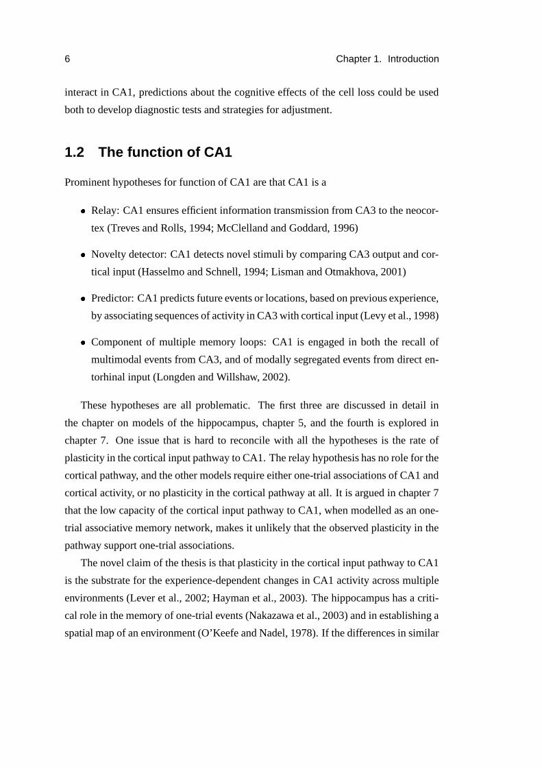
1.2 The function of CA1
Prominent hypotheses for function of CA1 are that CA1 is a
� Relay: CA1 ensures efficient information transmission from CA3 to the neocor-
tex (Treves and Rolls, 1994; McClelland and Goddard, 1996)
� Novelty detector: CA1 detects novel stimuli by comparing CA3 output and cor-
tical input (Hasselmo and Schnell, 1994; Lisman and Otmakhova, 2001)
� Predictor: CA1 predicts future events or locations, based on previous experience,
by associating sequences of activity in CA3 with cortical input (Levy et al., 1998)
� Component of multiple memory loops: CA1 is engaged in both the recall of
multimodal events from CA3, and of modally segregated events from direct en-
torhinal input (Longden and Willshaw, 2002).
These hypotheses are all problematic. The first three are discussed in detail in
the chapter on models of the hippocampus, chapter 5, and the fourth is explored in
chapter 7. One issue that is hard to reconcile with all the hypotheses is the rate of
plasticity in the cortical input pathway to CA1. The relay hypothesis has no role for the
cortical pathway, and the other models require either one-trial associations of CA1 and
cortical activity, or no plasticity in the cortical pathway at all. It is argued in chapter 7
that the low capacity of the cortical input pathway to CA1, when modelled as an one-
trial associative memory network, makes it unlikely that the observed plasticity in the
pathway support one-trial associations.
The novel claim of the thesis is that plasticity in the cortical input pathway to CA1
is the substrate for the experience-dependent changes in CA1 activity across multiple
environments (Lever et al., 2002; Hayman et al., 2003). The hippocampus has a criti-
cal role in the memory of one-trial events (Nakazawa et al., 2003) and in establishing a
spatial map of an environment (O’Keefe and Nadel, 1978). If the differences in similar
1.3. Approach 7
environments are not initially perceived, the activity corresponding to the memorised
events will be correlated through a shared representation of space. CA1 allows the rep-
resentations of the environments to become uncorrelated, as a function of experience,
whilst maintaining the memory of past events. This strategy allows the hippocampus
to support both the rapid acquisition of memories, and to benefit from experience in
developing perceptions of distinct spatial environments.
1.3 Approach
The proposed function of CA1 arises out of a process of constraining the existing hy-
pothesis space of CA1 function. From Marr (1971) onwards, pioneering models have
taken a top-down approach, stating a function for the hippocampus and then producing
computational and experimental evidence to support the hypothesis. This approach
has been very helpful and influential in establishing a conceptual framework both to
develop the computational ideas, and to interpret experimental results. Over thirty
years later, two major problems exist with the approach. The hypotheses generated by
these models have been very difficult to prove, because experiments must verify the
instantiation of high-level concepts. Secondly, the sheer volume of experimental data
means that very different positions have been maintained with a very slow progress to
resolution. This is particularly true for behavioural experiments, where the results are
exquisitely sensitive to the protocol used (Cohen and Eichenbaum, 1993).
Computational modelling is an appropriate tool for understanding the function of
CA1, because experimental manipulations of CA1 affect the whole hippocampal out-
put. Associative memory models of the hippocampus are the only kind which have
been able to account for the distinct anatomical organisation of the hippocampus.
The existing theories of CA1 function propose very different roles for the two in-
puts to CA1, from CA3 and directly from the neocortex. Using different modelling
approaches, I identify key properties of these pathways. These properties are used to
develop the hypothesis of CA1 function, in a bottom-up approach.
8 Chapter 1. Introduction
1.4 Thesis overview
Chapters 2, 3 and 4 present experimental findings which provide the context to the
discussion of the reviewed and proposed models of CA1. The claims and required
implementations of the models are diverse and overlapping. As a result, there are un-
avoidable, multiple narrative threads running through these chapters. Important themes
are
� Justification for associative memory models of the hippocampus
� Initial memory formation controlled by CA3 or cortical input
� Key features of CA1 and the cortical input assumed by current models, and
outwith current models.
Chapter 2 establishes the anatomy of the hippocampus relevant to the thesis. The
extrinsic connections of the hippocampus support an assumption of associative mem-
ory models, that the hippocampus associates patterns of activity from many cortical
areas. The intrinsic connections of CA1 constrain the mechanisms for generating pat-
terns of activity in CA1. It is also emphasised that the cortical input pathway is diver-
gent rather than the point-to-point mapping presumed by many models. Finally, the
organisation of the intrinsic entorhinal connections maintains the topographic organi-
sation of information modality, required by the hypothesis of multiple memory loops
through CA1.
Chapter 3 reviews the physiological properties of the cortical input pathway. It
was only recently established that long-term potentiation (LTP) and depression (LTD)
can be induced in the pathway (Remondes and Schuman, 2002; Dvorak-Carbone and
Schuman, 1999a). The timing of cortical stimulation and the induction of cortical
input LTP/D affect both the efficacy of CA3 stimulation in CA1, and the magnitude of
CA3-CA1 LTP/D in the slice (Remondes and Schuman, 2002; Levy et al., 1998). The
last topic discussed is the evidence for the activation of the cortical pathway, without
activating CA3, in support of the hypothesis for multiple memory loops through CA1.
Chapter 4 presents evidence for the two major behavioural correlates of hippocam-
pal activity in the rat: the memory of one-time experience and spatial learning. The
1.4. Thesis overview 9
origin of the memory hypothesis in human amnesia research is discussed, before re-
viewing attempts to produce experimental verification of a correlate in animals, specifi-
cally in rats. This is an important issue to verify for the associative memory modelling
in this thesis. The hippocampal dependence of spatial learning correlates with the
location-specific activity of hippocampal cells, known as place field activity. Through
observing place field formation, the formation of spatial memories can be observed.
In addition, the spatial activity of CA1 without CA3 activity is the only example of a
functional isolation of the cortical input to CA1 (Brun et al., 2002). Modelling is used
to constrain the mechanisms responsible for the results of Brun et al. (2002) in chap-
ter 9, in order to better understand the function of plasticity in the cortical pathway. In
readiness for that chapter, the spatial correlates of the cortical input and the long-term
changes to place fields are also discussed.
Chapter 5 reviews the computational models of the hippocampus that specify a
computational role for CA1. None of the models provide a compelling computational
reason for the entorhinal input to CA1. A key issue for the models is how patterns of
activity are formed in CA1: whether this process is controlled by Schaffer collateral
input, entorhinal input, or a combination of the two.
Chapter 6 provides a conceptual basis for discussing the formation of spatial mem-
ories in later chapters. The formation of place fields without CA3 (Brun et al., 2002) is
unlikely to be subserved by recurrent excitation or lateral inhibition (chapter 2). These
two mechanisms are utilised by all place field models except McHugh et al. (1996) and
Fuhs and Touretzky (2000). A cellular explanation of CA1 place field formation in the
cortical input pathway is developed in chapter 9.
In chapter 7, the model of Marr (1971) is used to provide evidence that CA1 main-
tains the transmission of information from CA3 to the neocortex (Treves and Rolls,
1994). First, the parameter dependencies of the performance advantage of multiple
layers in the pathways between the hippocampus and neocortex are identified. The
model is then applied to the network relaying activity from CA3 to the cortex and
subiculum. The capacity is quantifiably greater with CA1 than without CA1, over a
broad parameter range. From this it is concluded that CA1 improves the relay of infor-
mation from CA3 to the cortex and subiculum, supporting Treves (1995). The capacity
10 Chapter 1. Introduction
of the cortical pathway is calculated to be significantly lower than the CA3 input path-
way. It is concluded that the cortical pathway is unlikely to form associations at the
same rate as the CA3 pathway.
Chapter 8 investigates an algorithm proposed by Marr (1971) for pattern formation
in a partially connected feedforward network. The algorithm selects the output neurons
best connected to the input during memory storage. Analysis shows that networks with
patterns chosen this way have a higher capacity than network with random patterns, for
low connectivities and high memory loads. Simulations demonstrate that the superior
performance is maintained over a wider parameter range than specified by the analysis,
and when a more complex thresholding mechanism is used in the random network. The
possible implementation of the algorithm is the last topic of the chapter.
This position developed so far is difficult to reconcile with the hypotheses of CA1
as a novelty detector, predictor or component of mulitiple memory loops stated above.
The low capacity of the cortical compared to the CA3 input pathway indicates that
the rate of plasticity should be lower (chapter 7). The lower rate of cortical plasticity
is not consistent with recall from one-time events in the cortical pathway, and has an
as yet unspecified function if the cortical pathway establishes patterns of activity in
CA1. In addition, there are advantages of increased capacity and plausible implemen-
tation if CA3 chooses the most highly connected CA1 neurons during memory storage
(chapter 8).
Chapter 9 examines the computational requirements of forming place fields in the
cortical input pathway. Using an integrate-and-fire model of CA1, with a carefully
modelled entorhinal input, place field formation is shown to be robust to parameter
choices. When cortical input is mediated by small, temporally broad excitatory post-
synaptic potentials, place fields form despite an almost exclusively inhibitory response
to synchronous stimulation. It is argued that the high density of N-methyl-D-asparate
(NMDA) receptors at the cortical synapses (Otmakhova et al., 2002) supports the inte-
gration of spatially correlated cortical input.
Narrow place fields with high spatial information are supported by a large number
of cortical inputs with only small amounts of synaptic competition. Computing place
fields this way generates a synaptic weight distribution with limited generalisation of
1.4. Thesis overview 11
inputs in different environments. When this mechanism is combined with a scheme in
which CA3 input initially establishes CA1 activity, and cortical activity maintains this
activity, more decorrelated place maps of similar, distinct environments are formed.
This is consistent with the decorrelation of initially highly correlated spatial maps of
similar environments observed experimentally (Lever et al., 2002).
In the conclusion, chapter 10, the modelling results and their application to un-
derstanding the hippocampus are summarised. The hypothesis that plasticity in the
cortical pathway supports place field divergence in similar environments is discussed
in the light of emerging data indicating that CA1 activity is more likely to generalise
its representations over multiple environments than CA3. It is discussed how CA1 can
both learn the regularities and differences of multiple environments, and experimental
approaches to testing this hypothesis are discussed.

Chapter 2
Anatomy
2.1 Introduction
The emphasis of this review is on anatomical issues relevant to the models discussed
and developed in later chapters. Fundamental to the idea of associative memory mod-
els is the idea that the hippocampus is in an anatomical position to associate a diverse
set of sensory and non-sensory inputs. Within the hippocampus, establishing the con-
nectivity of CA1 is important for constraining the computational models. In particular,
the divergent nature of the temporoammonic input is discussed and the lack of recur-
rent collaterals in CA1 is discussed. Finally, the organisation of intrinsic entorhinal
connections is briefly discussed as an important component of the idea that activity
may reverberate through the entorhinal-CA1 network (Iijima et al., 1996; Longden
and Willshaw, 2002). Anatomical terminology that will recur throughout the thesis
has been labelled in bold font, for the ease of backreferencing. For clarity, anatomical
acronyms have not been used in the thesis.
2.2 Overview
The rat hippocampus is a prominent structure in both hemispheres of the brain, separat-
ing the neocortex and the lateral ventricle. Its distinctive banana shape has evoked im-
ages of seahorses and ram’s horns, inspiring the respective anatomical tags of the hip-
13

14 Chapter 2. Anatomy
pocampus in Greek (Aranzi, 1564) and cornu ammonis in Latin. Pioneering anatom-
ical surveys were performed by Schaffer (1892), Ramon y Cajal (1911, 1995) and
Lorente de No (1933, 1934) which immensely inspired subsequent research. Their
anatomical observations were refined using more modern techniques by Blackstad
(1956) and White (1959), heralding a new ‘golden age’ of hippocampal anatomy
(Amaral and Witter, 1995).
Locations along the hippocampus are tricky to describe because the anatomical
descriptions operate on linear axes. Two systems are in common usage, the septotem-
poral axis and the dorsoventral axis. The dorsal end closest to the septum, the dorsal
or septal pole, can be distinguished by its connection to a fibre bundle called the fornix.
The other end, ventrally located nearer the temporal cortex is the ventral or temporal
pole.
The transverse axis is perpendicular to the long axis, and it is in this plane that
the different anatomical regions of the hippocampus can be identified, on the basis of
different staining patterns. Lorente de No (1934) subdivided the hippocampus into the
area dentata and the cornu ammonis regions 1-4, the latter since abbreviated to CA1-4.
Area CA2 is small and usually ignored in the rodent literature, but ignored less often
in the primate literature. The area dentata is now called the dentate gyrus; older papers
refer to it as the fascia dentata (e.g. Marr, 1971). Blackstad (1956) identified CA4 as
part of the dentate gyrus, and defined it the hilus, the hilar region of the dentate gyrus.
Following Amaral and Witter (1995) I use the term hippocampus to refer to the
dentate gyrus and areas CA1, CA2 and CA3. Neighbouring the hippocampus are the
subiculum, presubiculum and parasubiculum. Like the hippocampus, these areas are
distinguished from the neocortex by having fewer than six layers.
2.3 Extrinsic connections
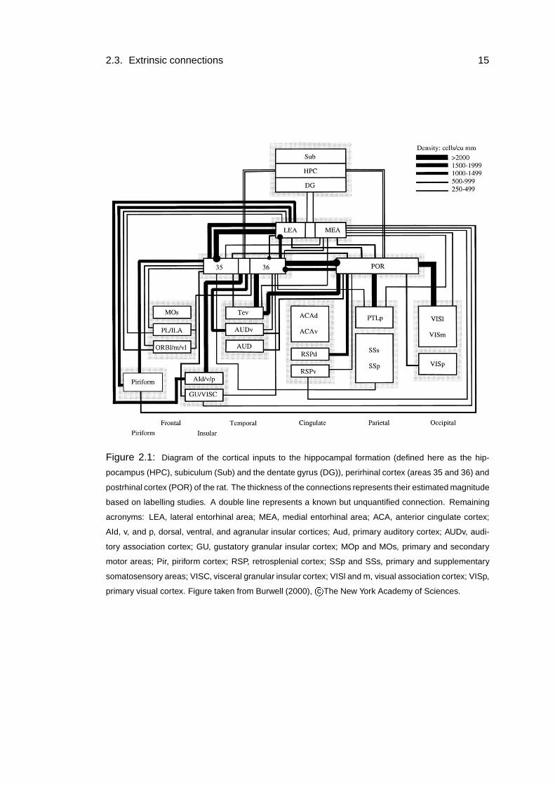
The major source of cortical afferents to the hippocampus is from the superficial layers
of the entorhinal cortex (Witter et al., 2000). Layer II neurons project to the dentate
gyrus and CA3, whilst layer III neurons project to CA1. Both of the projections are
collectively referred to as the perforant pathway. The fibres travel from the entorhinal
2.3. Extrinsic connections 15
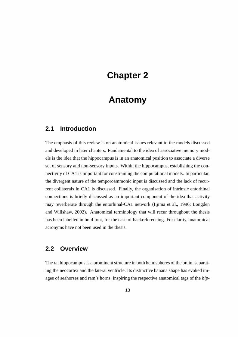
Figure 2.1: Diagram of the cortical inputs to the hippocampal formation (defined here as the hip-
pocampus (HPC), subiculum (Sub) and the dentate gyrus (DG)), perirhinal cortex (areas 35 and 36) and
postrhinal cortex (POR) of the rat. The thickness of the connections represents their estimated magnitude
based on labelling studies. A double line represents a known but unquantified connection. Remaining
acronyms: LEA, lateral entorhinal area; MEA, medial entorhinal area; ACA, anterior cingulate cortex;
AId, v, and p, dorsal, ventral, and agranular insular cortices; Aud, primary auditory cortex; AUDv, audi-
tory association cortex; GU, gustatory granular insular cortex; MOp and MOs, primary and secondary
motor areas; Pir, piriform cortex; RSP, retrosplenial cortex; SSp and SSs, primary and supplementary
somatosensory areas; VISC, visceral granular insular cortex; VISl and m, visual association cortex; VISp,
primary visual cortex. Figure taken from Burwell (2000), c�
The New York Academy of Sciences.
16 Chapter 2. Anatomy
cortex in a bundle that perforates the pyramidal layer of the subiculum.
In order to distinguish the perforant pathways throughout this thesis, I will refer to
the entorhinal-CA1 projection as the temporoammonic pathway, following previous
usage (Nadler et al., 1980; Maccaferri and McBain, 1995; Barbarosie et al., 2000; Re-
mondes and Schuman, 2002), and to the entorhinal-dentate gyrus and entorhinal-CA3
projections as the perforant pathway. The reader is warned that the term temporoam-
monic pathway is not yet established nomenclature, as very occasionally the term tem-
poroammonic pathway has been used to refer to the perforant path input to CA3 as
well (e.g. Tsukamoto et al., 2003).
The superficial entorhinal layers receive a large input from olfactory areas, includ-
ing the olfactory bulb and piriform (olfactory) cortex. The predominant cortical input
is to the superficial layers from the neighbouring perirhinal and postrhinal cortices.
The perirhinal and postrhinal cortices receive many cortical inputs, but especially from
differing regions of sensory association cortex (figure 2.1; Burwell, 2000). As a first
but accurate approximation, the hippocampus is the receiving peak of a pyramid of
sensory input.
The entorhinal cortex is also the principal cortical recipient of hippocampal output.
CA1 is the first and only hippocampal area to project back to the entorhinal cortex, to
the deep layers, predominantly layer V. The entorhinal cortex projects to a wide range
of cortical targets, but by far the most to the perirhinal cortex (Insausti et al., 1997).
The perirhinal cortex projects widely to many association and other cortices, including
the postrhinal cortex (figure 2.1).
CA1 is the major source of outputs from the hippocampus. It is a mistake to think of
the projections from CA1 simply as a relay back to the neocortical association areas,
as subcortical areas receive major projections from the hippocampus (fig. 2.2). The
biggest projection of CA1 is to the subiculum (Amaral and Witter, 1995). The main
projection of the subiculum is to subcortical areas, particularly the septal complex, the
mammillary nuclei, and the anterior thalamic complex (O’Mara et al., 2001). CA1
itself projects to subcortical areas, principally the lateral septum, receiving a lighter
return projection than the heavily septally innervated CA3. Other subcortical inputs
include the amygdala to the temporal third, and the thalamic nuclei.
2.4. Intrinsic organisation 17
Subiculum
EntorhinalCortexLayer II
CA3
PerforantPathway
DG
MossyFibrePathway
TemporoammonicPathway
RecurrentCollaterals
Schaffer Collaterals
CA1
Layer VI
Layer III
Layer V
Figure 2.2: Diagram of the connections of the hippocampus and the entorhinal cortex. The anatomical
connections indicate that cortical activity is transferred from the superficial layers of the entorhinal cortex,
through the dentate gyrus (DG), CA3, CA1 and subiculum. CA1 is the first hippocampal area with a
non-negligible projection back to the entorhinal cortex. The function of the projections from the deep to
superficial entorhinal cortex remain unknown.
A final reason to avoid viewing CA1 outputs as a relay to association cortices is
that the hippocampus and parahippocampal areas are intimately connected with the
prefrontal cortex (Delatour and Witter, 2002). A small but significant population of
CA1 and neurons project to the lateral and medial prefrontal cortex (Verwer et al.,
1997), and the subiculum projects heavily to the medial prefrontal cortex (Amaral and
Witter, 1995). The prefrontal cortex does not significantly project to the hippocam-
pus or subiculum directly, but enjoys reciprocal connections with the entorhinal and
parahippocampal cortices (Insausti et al., 1997; Delatour and Witter, 2002).
2.4 Intrinsic organisation
The granule cells, the excitatory cells of the dentate gyrus, project to CA3 via the
mossy fibres. The mossy fibres contact characteristically few CA3 pyramidal cells,
18 Chapter 2. Anatomy
� 46 (Amaral et al., 1990), and these synapses are very large. Some collaterals form
synapses with mossy cells, which provide a limited form of feedback to the granule
cells.
The pyramidal cells in CA3 receive the mossy fibre and perforant path input, and
form a large number of recurrent collaterals. The overall connectivity is � 4% (Li et al.,
1994), but because the collateral projections are spatially organised, every CA3 pyra-
midal cell can contact every other CA3 cell through 2-3 synaptic contacts (Amaral,
1993). The CA3 pyramidal cells also project ipsilaterally to the hilus, CA1, and con-
tralaterally to CA3 and CA1 (Li et al., 1994). The collaterals to CA1 are named the
Schaffer collaterals after Schaffer (1892).
One striking feature of CA1 is the low number of recurrent collaterals, certainly
compared to CA3 (Thomson and Radpour, 1991). Traub and Whittington (1999) es-
timate the probability of a connection to be � 1%, based on the data of Deuchars and
Thomson (1996) who recorded from 989 pairs of CA1 pyramidal cells and found that 9
pairs were monosynaptically connected. Only the local connectivity can be estimated
to be � 1% because this is in the slice. There is little quantitative data on the number
and spatial distribution of pyramidal cell recurrent collaterals because there are so few.
In a study of the CA1 axonal projections using an anterograde tracer, only ‘meager’
recurrent collateral staining is found, and this is mainly adjacent to the injection site
(Amaral et al., 1991). Closer inspection reveals recurrent collaterals that cover � 2
mm of the septotemporal axis of CA1. Given a septotemporal length of � 10 mm,
this would reduce the estimate to � 0.2%. Similarly, the number of CA1 contralateral
connections is low compared to CA3 (Amaral and Witter, 1995).
The recurrent collaterals project to the stratum oriens, where proportionately few
of the excitatory inputs to parvalbumin positive basket and chandelier cells are located
(Gulyas et al., 1999). After ischaemia, stratum oriens interneurons are revealed to
be the principal targets of the degenerating recurrent collaterals, which are the most
vulnerable to damage (Blasco-Ibanez and Freund, 1995). During sharp wave ripples
(140-200 Hz activity), CA1 pyramidal cells are synchronously highly active and the ac-
tivity of interneurons in the strata pyramidale and oriens follows 1-2 ms later (Csicsvari
et al., 1998). This indicates that basket, chandelier and stratum oriens interneurons can
2.4. Intrinsic organisation 19
Entorhinal
layer IIICortex
MoleculareStratum Lacunosum−
Stratum Pyramidale
Stratum Oriens
Temporoammonic pathway
Schaffer collaterals
Pyramidal cell body
Recurrent collaterals
CA3
Stratum Radiatum
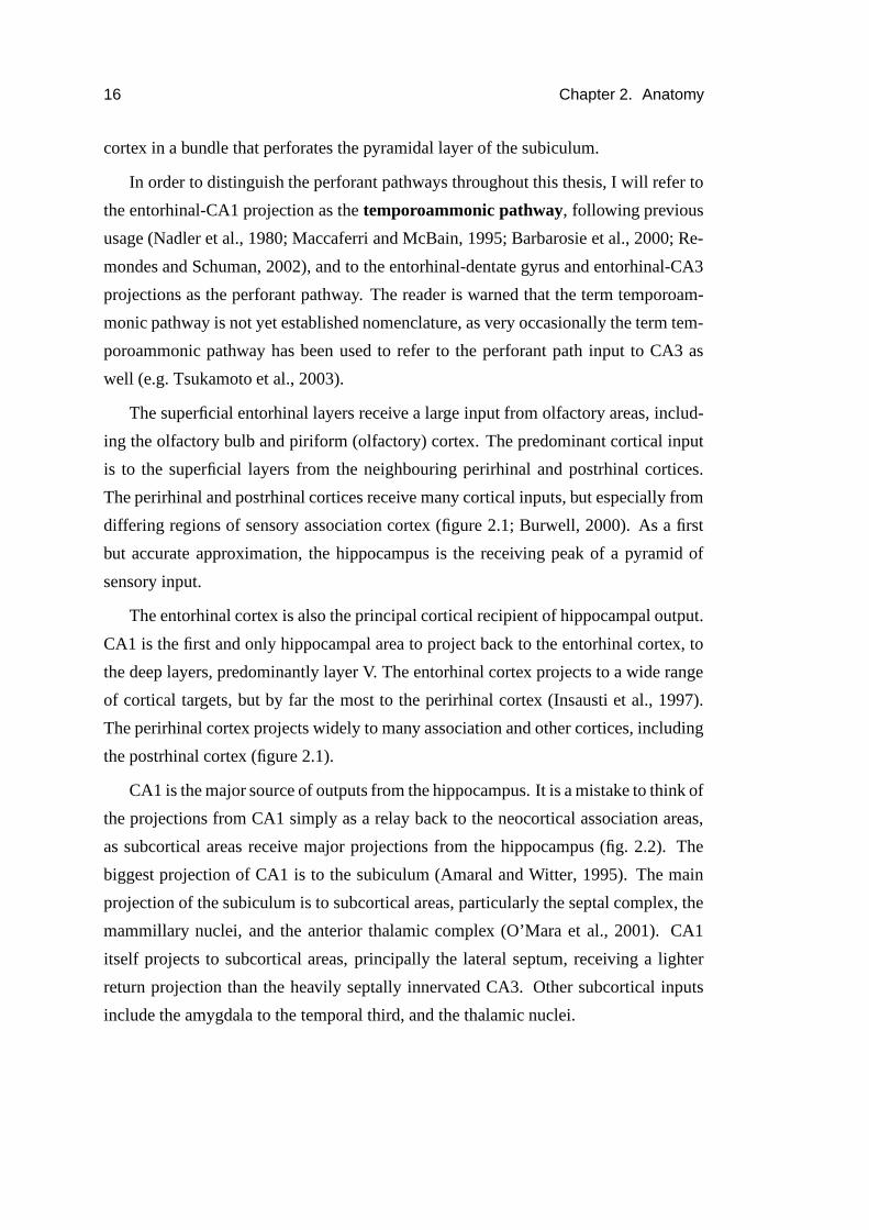
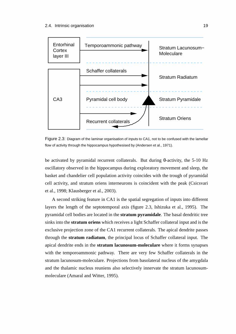
Figure 2.3: Diagram of the laminar organisation of inputs to CA1, not to be confused with the lamellar
flow of activity through the hippocampus hypothesised by (Andersen et al., 1971).
be activated by pyramidal recurrent collaterals. But during θ-activity, the 5-10 Hz
oscillatory observed in the hippocampus during exploratory movement and sleep, the
basket and chandelier cell population activity coincides with the trough of pyramidal
cell activity, and stratum oriens interneurons is coincident with the peak (Csicsvari
et al., 1998; Klausberger et al., 2003).
A second striking feature in CA1 is the spatial segregation of inputs into different
layers the length of the septotemporal axis (figure 2.3, Ishizuka et al., 1995). The
pyramidal cell bodies are located in the stratum pyramidale. The basal dendritic tree
sinks into the stratum oriens which receives a light Schaffer collateral input and is the
exclusive projection zone of the CA1 recurrent collaterals. The apical dendrite passes
through the stratum radiatum, the principal locus of Schaffer collateral input. The
apical dendrite ends in the stratum lacunosum-moleculare where it forms synapses
with the temporoammonic pathway. There are very few Schaffer collaterals in the
stratum lacunosum-moleculare. Projections from basolateral nucleus of the amygdala
and the thalamic nucleus reuniens also selectively innervate the stratum lacunosum-
moleculare (Amaral and Witter, 1995).
20 Chapter 2. Anatomy
2.5 Topographic organisation of CA1 inputs and out-
puts
There is a recurring, strong assumption in the modelling literature that the temporoam-
monic pathway is a highly ordered, ‘point-to-point’ mapping (Hasselmo and Schnell,
1994; McClelland and Goddard, 1996; Lisman, 1999; Lorincz and Buzsaki, 2000).
The original idea of point-to-point mappings in the hippocampus was introduced by
Andersen et al. (1971). They orthodromically and antidromically stimulated the per-
forant path projection to the dentate gyrus, the mossy fibre pathway, and the Schaffer
collaterals. The spatial locations of the population spikes indicated that information
flowed around the trisynaptic loop in narrow transverse slices, stacked along the long
axis. This arrangement of essentially independent units is referred to as the ‘lamellar
organisation’ of the hippocampus (Amaral and Witter, 1989).
Whilst the mossy fibre projection does indeed appear to be lamellar, subsequent
anatomical work has taken great pains to point out that the perforant path projections
to the dentate gyrus and the Schaffer collaterals are far from lamellar (Amaral and
Witter, 1989). The perforant path is highly divergent, with � 10% of the length of the
entorhinal cortex (along its corresponding medial-lateral axis) projecting to � 40% of
the length of the dentate gyrus, densely over 25% of the length (Amaral and Witter,
1989; Dolorfo and Amaral, 1998a). The divergence of the Schaffer collaterals is even
greater: one cited example contacted � 90% of the length of CA1 from staining � 10%
of the septotemporal length of CA3 (Ishizuka et al., 1990), but the average length is� 60% of the longitudinal axis of CA1 (Li et al., 1994; Ishizuka et al., 1990). This
kind of divergence is sufficiently large that it is unlikely to be explained by the need
for projections to support wide field inhibition around an excitatory peak.
These results set up a dialectic between the ideas of a lamellar and a highly diver-
gent projection. In truth there is a graded spectrum: the mossy fibres are lamellar, the
perforant path to the dentate gyrus is divergent, and the Schaffer collaterals are highly
divergent. In this context, the topographical organisation of the projections from CA1
to the subiculum and deep entorhinal cortex has recently been emphasised (Tamamaki
and Nojyo, 1995; Burwell, 2000; Witter et al., 2000; Naber et al., 2001). The topo-
2.5. Topographic organisation of CA1 inputs and outputs 21
graphic mapping is along the transverse axis: the medial entorhinal cortex projects to
CA1 proximal to the dentate gyrus, whilst the lateral entorhinal cortex projects to CA1
distal from the dentate gyrus. Retrogradedly labelled entorhinal cells in CA1 covered
approximately one third of the proximodistal axis (Tamamaki and Nojyo, 1995). This
is consistent with the projection, for instance, from CA1 to the subiculum: the prox-
imal third of CA1 projects to the distal third of the subiculum, and the distal third of
CA1 projects to the proximal third of the subiculum (Witter et al., 2000).
This organisation is maintained throughout the connections between the hippocam-
pus, subiculum, entorhinal cortex, and parasubicular areas (Burwell, 2000; Naber et al.,
2001). As discussed above, the perirhinal and postrhinal cortices receive different
modalities of sensory input. In principle, these connections create loops that could
preserve the modality of transmitted activity. In contrast, the Schaffer collateral pro-
jection is organised such that any CA3 pyramidal cell can contact any CA1 cell (Li
et al., 1994). The CA1 cells therefore receive modality mixed information from these
pathways. This lack of topographical organisation was also believed to apply to the
perforant path projection to the dentate gyrus (Amaral and Witter, 1989). Recently
Dolorfo and Amaral (1998b) reported remarkably little spatial overlap in the domains
of entorhinal cells projecting to distinct septotemporal thirds of the dentate gyrus.
The significance of the topography of the temporoammonic pathway is that it al-
lows only restricted combinations of input, and positively not that the projection is
not divergent. The divergency of the temporoammonic pathway at � 33% is roughly
equal to the divergence of the perforant path input to the dentate gyrus at 25% � 40%.
The fact that it is less than the Schaffer collaterals does not imply that it should in any
way be thought of as a ‘point-to-point’. Common references used in support of this
point are the work of Tamamaki and colleagues, culminating in Tamamaki and Nojyo
(1995), as referenced by O’Reilly and McClelland (1994), Lisman (1999) and Lorincz
and Buzsaki (2000). Tamamaki and Nojyo (1995) explicitly state “...these three fields
[subiculum, CA1, and entorhinal cortex] do not represent a point-to-point topography
but diverge in each direction.”
In order to support claims of a point-to-point mapping, electrophysiological record-
ings would be required to demonstrate a narrow field of excitatory response as found
22 Chapter 2. Anatomy
by Andersen et al. (1971) in the Schaffer collaterals. Recordings at numerous but un-
systematically varied sites along the length of CA1 in vitro reveal uniformly inhibitory
somatic responses (Soltesz, 1995). This does not preclude centre-surround response, as
the excitatory response may have been missed, but certainly does not provide evidence
in support of point-to-point mapping.
2.6 Intrinsic connections of the entorhinal cortex
The predominate pattern of intrinsic projections in the entorhinal cortex is from the
deep to the superficial layers (Dolorfo and Amaral, 1998a). Since the deep layers of
the entorhinal cortex are the primary cortical recipients of hippocampal output, and the
superficial layers are the primary source of hippocampal input, this raises the possibil-
ity that the entorhinal cortex may facilitate hippocampal reverberations (Iijima et al.,
1996; Longden and Willshaw, 2002). The intrinsic deep to superficial entorhinal con-
nections are mostly restricted to three areas defined by the dorsoventral and rostrocau-
dal axes. These areas are partially but not completely in register with the topographic
organisation of the projections between the entorhinal cortex, CA1, subiculum and
parahippocampal areas.
In contrast to the point-to-point hypothesis of the temporoammonic pathway, both
the deep-deep and lighter superficial-superficial intrinsic projections are divergent within
their bands. Axons of cells injected with Phaseolus vulgaris-leuocoagglutinin (PHA-
L) reveal heavy staining within every band, and moderate to light staining between
bands (Dolorfo and Amaral, 1998a). On the basis of this evidence, the entorhinal input
to CA1 contains an admixture of hippocampal output from within the (mildly) segre-
gated entorhinal target zone of the CA1 afferents.
Chapter 3
Physiology of the temporoammonic
pathway
3.1 Introduction
The nature of the temporoammonic input to CA1 lies at the heart of CA1 information
processing. An important issue for understanding the mystery is establishing how
useful information processing can occur in the temporoammonic pathway, when its
stimulation results in a large, widespread inhibitory somatic response. It is argued in
section 9.3 that the recent discovery of high levels of NMDA receptors (NMDARs) in
the temporoammonic synapses of pyramidal cells (Otmakhova et al., 2002) can explain
this inhibitory response.
Brun et al. (2002) observed behaviourally significant location-specific activity in
CA1 without CA3 input. Does this imply that temporoammonic input controls place
field firing in the presence of CA3 input? This intriguing concept is a tenet of most
hippocampal models that include a representation of CA1. Remondes and Schuman
(2002) provide tantalising physiological data as to how this control maybe maintained.
The relative timing of temporoammonic stimulation not only affects Schaffer collateral
efficacy, but plasticity too, and both effects are themselves modulated by temporoam-
monic plasticity. The observation of behaviourally relevant activity in CA1 from tem-
poroammonic input alone (Brun et al., 2002), despite the almost exclusively inhibitory
23
24 Chapter 3. Physiology of the temporoammonic pathway
Moleculare
Stratum
pathway
Stratum
Stratum
Stratum
collaterals
Lacunosum−
Temporoammonic
Radiatum
Pyramidale
Oriens
Schaffer
LM
CC BS BC
OLM
PC
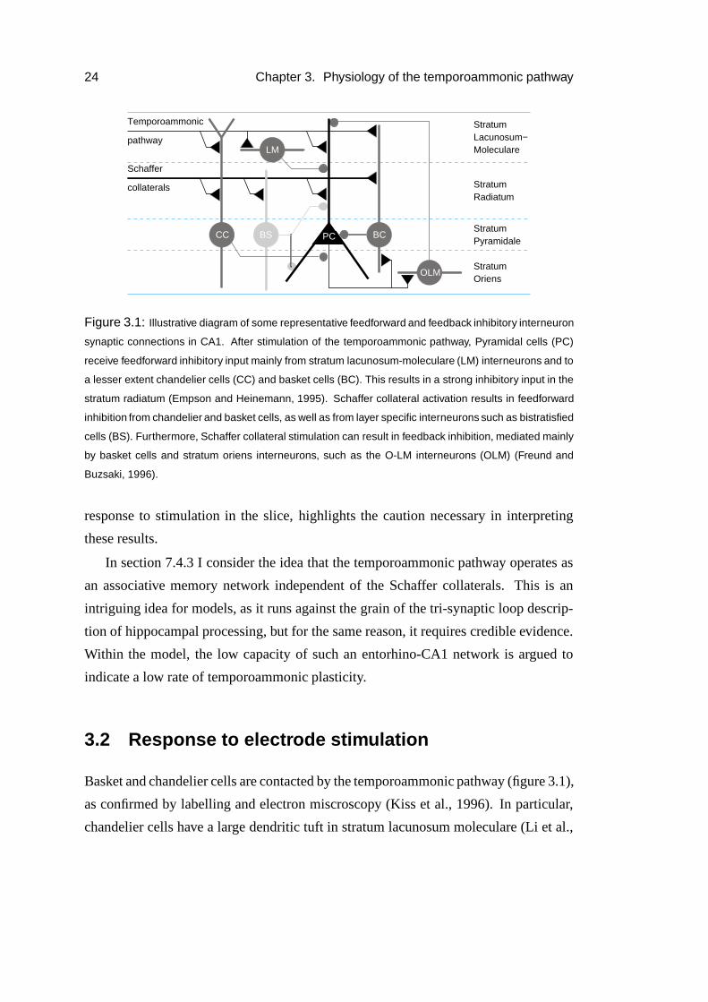
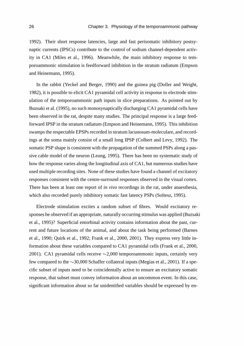
Figure 3.1: Illustrative diagram of some representative feedforward and feedback inhibitory interneuron
synaptic connections in CA1. After stimulation of the temporoammonic pathway, Pyramidal cells (PC)
receive feedforward inhibitory input mainly from stratum lacunosum-moleculare (LM) interneurons and to
a lesser extent chandelier cells (CC) and basket cells (BC). This results in a strong inhibitory input in the
stratum radiatum (Empson and Heinemann, 1995). Schaffer collateral activation results in feedforward
inhibition from chandelier and basket cells, as well as from layer specific interneurons such as bistratisfied
cells (BS). Furthermore, Schaffer collateral stimulation can result in feedback inhibition, mediated mainly
by basket cells and stratum oriens interneurons, such as the O-LM interneurons (OLM) (Freund and
Buzsaki, 1996).
response to stimulation in the slice, highlights the caution necessary in interpreting
these results.
In section 7.4.3 I consider the idea that the temporoammonic pathway operates as
an associative memory network independent of the Schaffer collaterals. This is an
intriguing idea for models, as it runs against the grain of the tri-synaptic loop descrip-
tion of hippocampal processing, but for the same reason, it requires credible evidence.
Within the model, the low capacity of such an entorhino-CA1 network is argued to
indicate a low rate of temporoammonic plasticity.
3.2 Response to electrode stimulation
Basket and chandelier cells are contacted by the temporoammonic pathway (figure 3.1),
as confirmed by labelling and electron miscroscopy (Kiss et al., 1996). In particular,
chandelier cells have a large dendritic tuft in stratum lacunosum moleculare (Li et al.,
3.2. Response to electrode stimulation 25
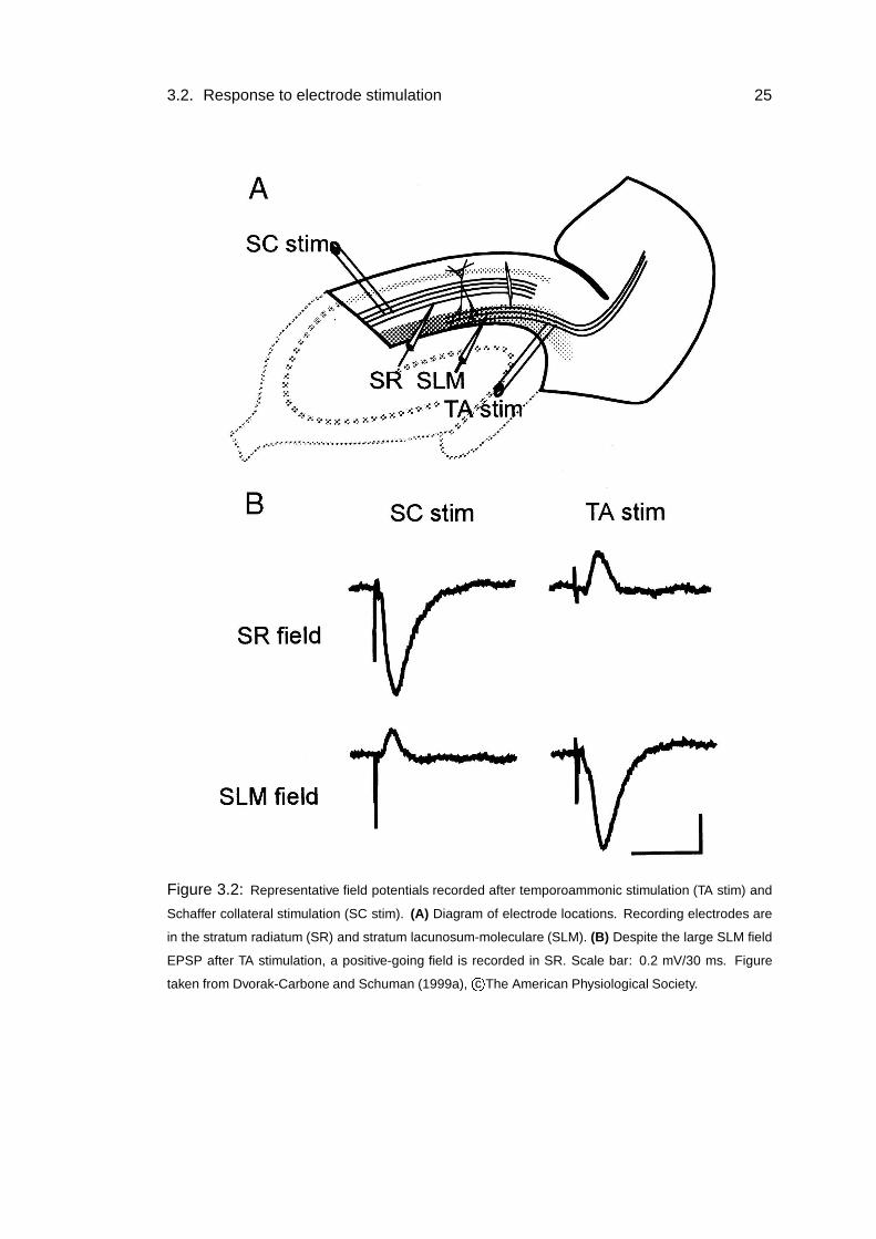
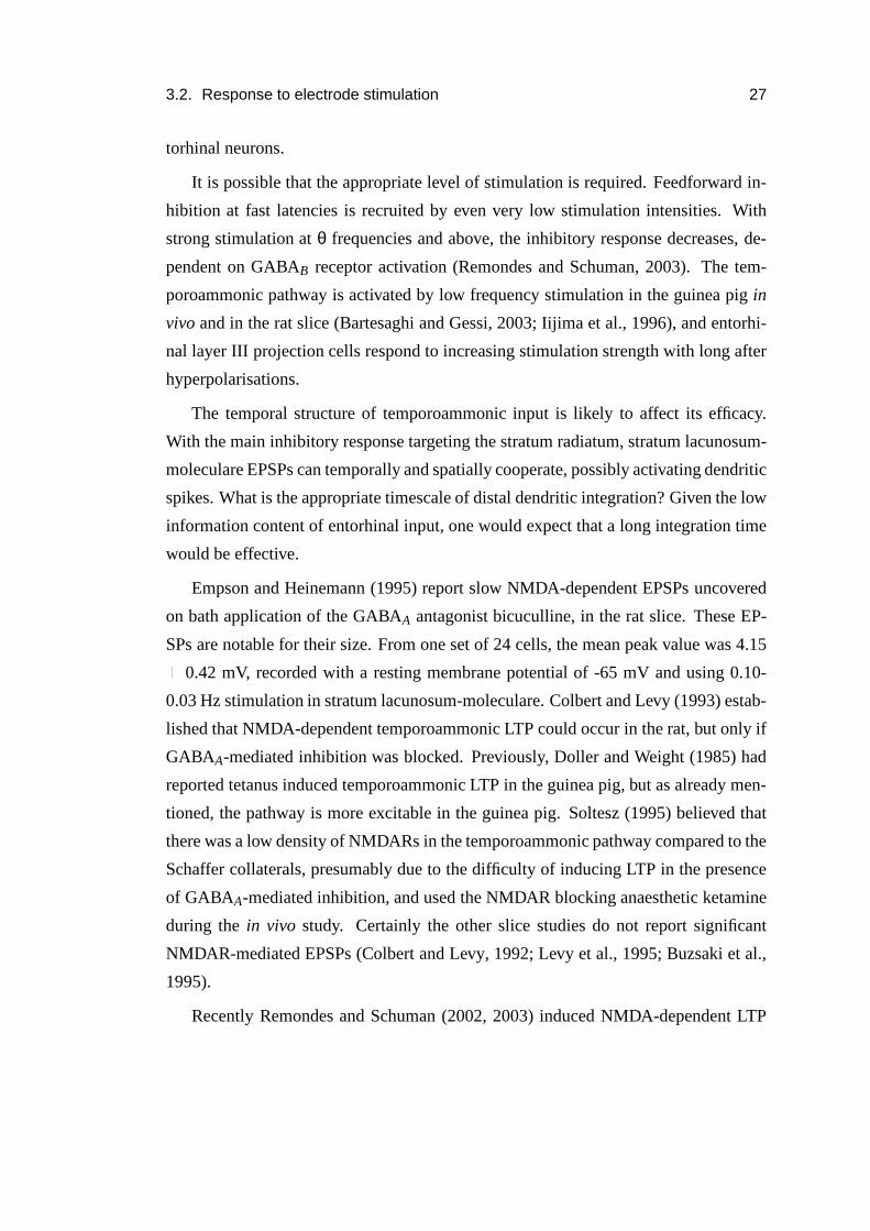
Figure 3.2: Representative field potentials recorded after temporoammonic stimulation (TA stim) and
Schaffer collateral stimulation (SC stim). (A) Diagram of electrode locations. Recording electrodes are
in the stratum radiatum (SR) and stratum lacunosum-moleculare (SLM). (B) Despite the large SLM field
EPSP after TA stimulation, a positive-going field is recorded in SR. Scale bar: 0.2 mV/30 ms. Figure
taken from Dvorak-Carbone and Schuman (1999a), c�
The American Physiological Society.
26 Chapter 3. Physiology of the temporoammonic pathway
1992). Their short response latencies, large and fast perisomatic inhibitory postsy-
naptic currents (IPSCs) contribute to the control of sodium channel-dependent activ-
ity in CA1 (Miles et al., 1996). Meanwhile, the main inhibitory response to tem-
poroammonic stimulation is feedforward inhibition in the stratum radiatum (Empson
and Heinemann, 1995).
In the rabbit (Yeckel and Berger, 1990) and the guinea pig (Doller and Weight,
1982), it is possible to elicit CA1 pyramidal cell activity in response to electrode stim-
ulation of the temporoammonic path inputs in slice preparations. As pointed out by
Buzsaki et al. (1995), no such monosynaptically discharging CA1 pyramidal cells have
been observed in the rat, despite many studies. The principal response is a large feed-
forward IPSP in the stratum radiatum (Empson and Heinemann, 1995). This inhibition
swamps the respectable EPSPs recorded in stratum lacunosum-moleculare, and record-
ings at the soma mainly consist of a small long IPSP (Colbert and Levy, 1992). The
somatic PSP shape is consistent with the propagation of the summed PSPs along a pas-
sive cable model of the neuron (Leung, 1995). There has been no systematic study of
how the response varies along the longitudinal axis of CA1, but numerous studies have
used multiple recording sites. None of these studies have found a channel of excitatory
responses consistent with the centre-surround responses observed in the visual cortex.
There has been at least one report of in vivo recordings in the rat, under anaesthesia,
which also recorded purely inhibitory somatic fast latency PSPs (Soltesz, 1995).
Electrode stimulation excites a random subset of fibres. Would excitatory re-
sponses be observed if an appropriate, naturally occurring stimulus was applied (Buzsaki
et al., 1995)? Superficial entorhinal activity contains information about the past, cur-
rent and future locations of the animal, and about the task being performed (Barnes
et al., 1990; Quirk et al., 1992; Frank et al., 2000, 2001). They express very little in-
formation about these variables compared to CA1 pyramidal cells (Frank et al., 2000,
2001). CA1 pyramidal cells receive � 2,000 temporoammonic inputs, certainly very
few compared to the � 30,000 Schaffer collateral inputs (Megıas et al., 2001). If a spe-
cific subset of inputs need to be coincidentally active to ensure an excitatory somatic
response, that subset must convey information about an uncommon event. In this case,
significant information about so far unidentified variables should be expressed by en-
3.2. Response to electrode stimulation 27
torhinal neurons.
It is possible that the appropriate level of stimulation is required. Feedforward in-
hibition at fast latencies is recruited by even very low stimulation intensities. With
strong stimulation at θ frequencies and above, the inhibitory response decreases, de-
pendent on GABAB receptor activation (Remondes and Schuman, 2003). The tem-
poroammonic pathway is activated by low frequency stimulation in the guinea pig in
vivo and in the rat slice (Bartesaghi and Gessi, 2003; Iijima et al., 1996), and entorhi-
nal layer III projection cells respond to increasing stimulation strength with long after
hyperpolarisations.
The temporal structure of temporoammonic input is likely to affect its efficacy.
With the main inhibitory response targeting the stratum radiatum, stratum lacunosum-
moleculare EPSPs can temporally and spatially cooperate, possibly activating dendritic
spikes. What is the appropriate timescale of distal dendritic integration? Given the low
information content of entorhinal input, one would expect that a long integration time
would be effective.
Empson and Heinemann (1995) report slow NMDA-dependent EPSPs uncovered
on bath application of the GABAA antagonist bicuculline, in the rat slice. These EP-
SPs are notable for their size. From one set of 24 cells, the mean peak value was 4.15�
0.42 mV, recorded with a resting membrane potential of -65 mV and using 0.10-
0.03 Hz stimulation in stratum lacunosum-moleculare. Colbert and Levy (1993) estab-
lished that NMDA-dependent temporoammonic LTP could occur in the rat, but only if
GABAA-mediated inhibition was blocked. Previously, Doller and Weight (1985) had
reported tetanus induced temporoammonic LTP in the guinea pig, but as already men-
tioned, the pathway is more excitable in the guinea pig. Soltesz (1995) believed that
there was a low density of NMDARs in the temporoammonic pathway compared to the
Schaffer collaterals, presumably due to the difficulty of inducing LTP in the presence
of GABAA-mediated inhibition, and used the NMDAR blocking anaesthetic ketamine
during the in vivo study. Certainly the other slice studies do not report significant
NMDAR-mediated EPSPs (Colbert and Levy, 1992; Levy et al., 1995; Buzsaki et al.,
1995).
Recently Remondes and Schuman (2002, 2003) induced NMDA-dependent LTP

28 Chapter 3. Physiology of the temporoammonic pathway
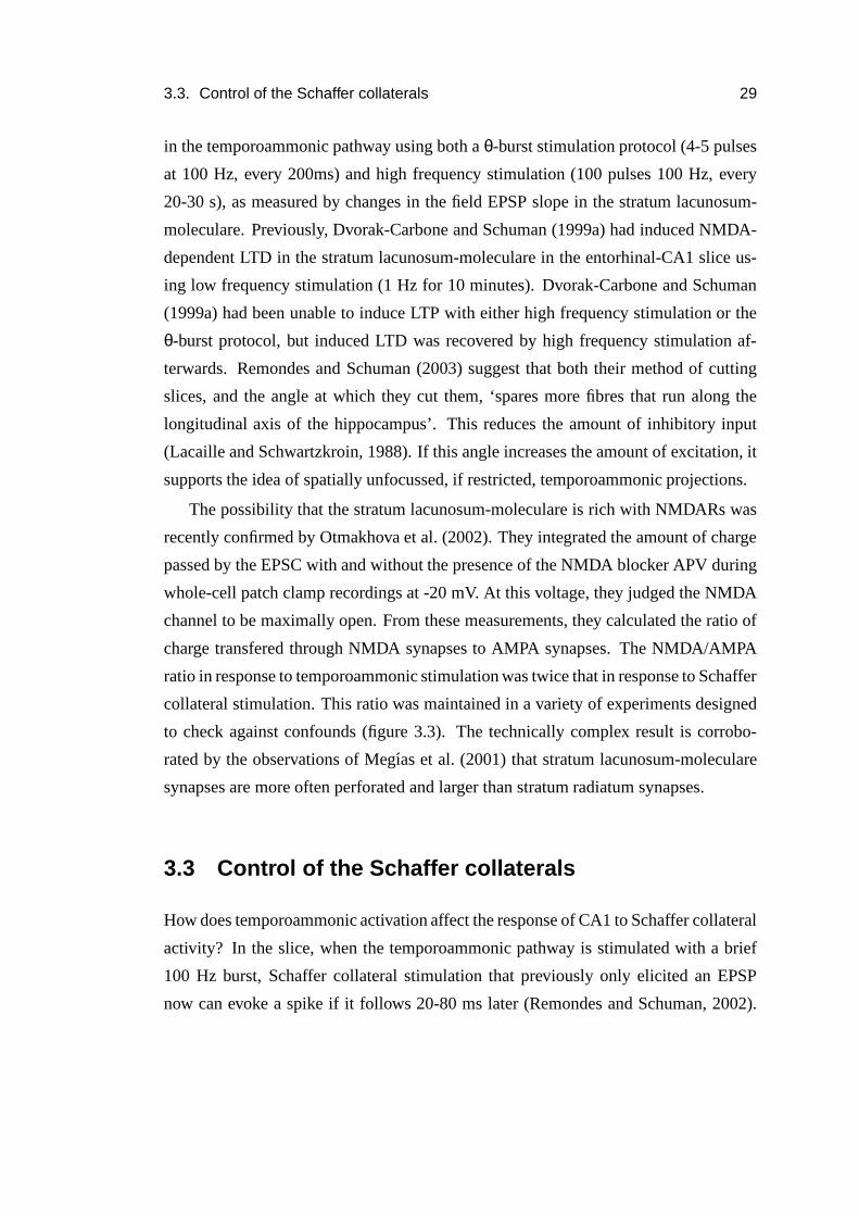
Figure 3.3: NMDA/AMPA area ratio of temporoammonic (here perforant path, PP) EPSPs is � double
the ratio for Schaffer collateral (SC) EPSPs. Results of a cell body patch clamp experiment in slices in
artificial cerebrospinal fluid either with magnesium (control) or without (Low Mg2�
. Picrotoxin (PTX) is
added to block GABA receptors, and APV is an NMDAR antagonist. (A) Averages of 10 EPSPs. (B)
Total area of EPSPs from 11 cells. Asterisks denote significant difference from the previous condition
(*p � 0.05, **p � 0.01). Figure taken from Otmakhova et al. (2002), c�
Society for Neuroscience.
3.3. Control of the Schaffer collaterals 29
in the temporoammonic pathway using both a θ-burst stimulation protocol (4-5 pulses
at 100 Hz, every 200ms) and high frequency stimulation (100 pulses 100 Hz, every
20-30 s), as measured by changes in the field EPSP slope in the stratum lacunosum-
moleculare. Previously, Dvorak-Carbone and Schuman (1999a) had induced NMDA-
dependent LTD in the stratum lacunosum-moleculare in the entorhinal-CA1 slice us-
ing low frequency stimulation (1 Hz for 10 minutes). Dvorak-Carbone and Schuman
(1999a) had been unable to induce LTP with either high frequency stimulation or the
θ-burst protocol, but induced LTD was recovered by high frequency stimulation af-
terwards. Remondes and Schuman (2003) suggest that both their method of cutting
slices, and the angle at which they cut them, ‘spares more fibres that run along the
longitudinal axis of the hippocampus’. This reduces the amount of inhibitory input
(Lacaille and Schwartzkroin, 1988). If this angle increases the amount of excitation, it
supports the idea of spatially unfocussed, if restricted, temporoammonic projections.
The possibility that the stratum lacunosum-moleculare is rich with NMDARs was
recently confirmed by Otmakhova et al. (2002). They integrated the amount of charge
passed by the EPSC with and without the presence of the NMDA blocker APV during
whole-cell patch clamp recordings at -20 mV. At this voltage, they judged the NMDA
channel to be maximally open. From these measurements, they calculated the ratio of
charge transfered through NMDA synapses to AMPA synapses. The NMDA/AMPA
ratio in response to temporoammonic stimulation was twice that in response to Schaffer
collateral stimulation. This ratio was maintained in a variety of experiments designed
to check against confounds (figure 3.3). The technically complex result is corrobo-
rated by the observations of Megıas et al. (2001) that stratum lacunosum-moleculare
synapses are more often perforated and larger than stratum radiatum synapses.
3.3 Control of the Schaffer collaterals
How does temporoammonic activation affect the response of CA1 to Schaffer collateral
activity? In the slice, when the temporoammonic pathway is stimulated with a brief
100 Hz burst, Schaffer collateral stimulation that previously only elicited an EPSP
now can evoke a spike if it follows 20-80 ms later (Remondes and Schuman, 2002).
30 Chapter 3. Physiology of the temporoammonic pathway
In contrast, when Schaffer collateral stimulation just strong enough to consistently
evoke a spike follows by 200 ms or more, the probability of evoking a spike is signif-
icantly reduced (Dvorak-Carbone and Schuman, 1999b). This ‘spike-blocking’ has a
time course consistent with GABAB receptors, and indeed is itself blocked by GABAB
receptor antagonists. Unfortunately, due to the complex localisations of presynaptic,
postsynaptic and extrasynaptic GABAB receptors around Schaffer collateral synapses
(Colbert and Levy, 1992; Scanziani, 2000; Pham et al., 1998), the mechanism remains
unknown. In turn, it is difficult to predict whether or not it occurs during the rhythmic
discharge of interneurons during θ-activity.
The relative timing of temporoammonic and Schaffer collateral stimulation also
affects the induction of LTP in the Schaffer collaterals. When stimulated at the same
time with brief, high frequency spike trains, the change in the slope of the field EPSP
was significantly less than when the Schaffer collaterals were stimulated alone (Levy
et al., 1998). This reduction in LTP is blocked by the GABAA antagonist bicuculline
(Remondes and Schuman, 2002).
The GABAB receptor anatagonist CGP blocks temporoammonic LTP (Remondes
and Schuman, 2003). Similar effects have been reported at Schaffer collateral synapses
(Davies et al., 1991), and at perforant path synapses to dentate granule cells (Mott and
Lewis, 1991), where presynaptic GABAB receptors on inhibitory synapses are autoac-
tivated. Without the resulting disinhibition, LTP induction is blocked. The Schaffer
collateral synapses also have presynaptic GABAB receptors, whereas the temporoam-
monic synapses do not (Colbert and Levy, 1992). The unknown factor is what levels
of inhibitory activity are required to activate these presynaptic GABAB receptors and
facilitate LTP.
Once induced, temporoammonic LTP has fascinating implications for Schaffer col-
lateral activation. After the induction of temporoammonic LTP using the high fre-
quency protocol, the magnitude of both spike-blocking and enhancing of Schaffer col-
lateral stimulation by appropriately timed temporoammonic stimulation were signif-
icantly increased (Remondes and Schuman, 2002). Meanwhile, after the induction
of LTD, the magnitude of the spike-blocking and enhancement were significantly de-
creased. Furthermore, after temporoammonic LTP, the magnitude of the reduction
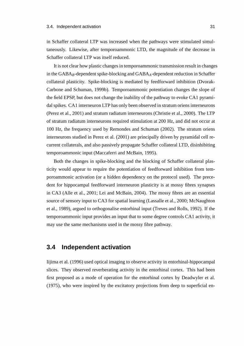
3.4. Independent activation 31
in Schaffer collateral LTP was increased when the pathways were stimulated simul-
taneously. Likewise, after temporoammonic LTD, the magnitude of the decrease in
Schaffer collateral LTP was itself reduced.
It is not clear how plastic changes in temporoammonic transmission result in changes
in the GABAB-dependent spike-blocking and GABAA-dependent reduction in Schaffer
collateral plasticity. Spike-blocking is mediated by feedforward inhibition (Dvorak-
Carbone and Schuman, 1999b). Temporoammonic potentiation changes the slope of
the field EPSP, but does not change the inability of the pathway to evoke CA1 pyrami-
dal spikes. CA1 interneuron LTP has only been observed in stratum oriens interneurons
(Perez et al., 2001) and stratum radiatum interneurons (Christie et al., 2000). The LTP
of stratum radiatum interneurons required stimulation at 200 Hz, and did not occur at
100 Hz, the frequency used by Remondes and Schuman (2002). The stratum oriens
interneurons studied in Perez et al. (2001) are principally driven by pyramidal cell re-
current collaterals, and also passively propagate Schaffer collateral LTD, disinhibiting
temporoammonic input (Maccaferri and McBain, 1995).
Both the changes in spike-blocking and the blocking of Schaffer collateral plas-
ticity would appear to require the potentiation of feedforward inhibition from tem-
poroammonic activation (or a hidden dependency on the protocol used). The prece-
dent for hippocampal feedforward interneuron plasticity is at mossy fibres synapses
in CA3 (Alle et al., 2001; Lei and McBain, 2004). The mossy fibres are an essential
source of sensory input to CA3 for spatial learning (Lassalle et al., 2000; McNaughton
et al., 1989), argued to orthogonalise entorhinal input (Treves and Rolls, 1992). If the
temporoammonic input provides an input that to some degree controls CA1 activity, it
may use the same mechanisms used in the mossy fibre pathway.
3.4 Independent activation
Iijima et al. (1996) used optical imaging to observe activity in entorhinal-hippocampal
slices. They observed reverberating activity in the entorhinal cortex. This had been
first proposed as a mode of operation for the entorhinal cortex by Deadwyler et al.
(1975), who were inspired by the excitatory projections from deep to superficial en-
32 Chapter 3. Physiology of the temporoammonic pathway
torhinal cortex. Excitingly, Iijima et al. (1996) also observed frequency dependent
transmission of activity to the hippocampus. This latter observation was repeated in
rat slices (Gloveli et al., 1997b). The entorhinal layer II projections to CA3 and the
dentate gyrus are preferentially activated by stimulus frequencies above 5 Hz, and re-
main inactive for lower stimulus frequencies. In contrast, entorhinal layer II neurons
are preferentially activated by frequencies below 10 Hz, and are strongly inhibited at
higher frequencies. In anaesthetised guinea pigs, Bartesaghi and Gessi (2003) found
that for 1-4 Hz stimuli, a current sink was observed in CA1 alone in the hippocampus.
In anaesthetised rats, 0.15 Hz stimulation of CA3 resulted in a current sink in the mid-
dle molecular layer of the dentate gyrus, corresponding to the projection zone of the
medial perforant path (Canning et al., 2000).
These findings are consistent with the electrophysiology of entorhinal layer II and
III projection neurons. In layer II projection neurons, postsynaptic NMDARs facilitate
an increased probability of an action potential with repeated stimulation (Heinemann
et al., 2000). In contrast, repetitive stimulation results in a long hyperpolarisation in
layer III projection neurons (Gloveli et al., 1997a).
If activity can reverberate in a frequency dependent manner either through the trisy-
naptic circuit, or through the temporoammonic pathway, one would expect the two
reverberatory loops to have differentiable functions. Sybirska et al. (2000) used 2-
deoxyglucose imaging to observe metabolic activity in the hippocampi of rhesus mon-
keys during delayed match-to-sample and oculomotor delayed-response tasks. The
method preferentially labels the activity in active axonal arbourisations. In all tasks,
they observed intense activity in the stratum lacunosum-moleculare of CA1, but little
activity in CA3. The authors infer that the temporoammonic pathway is recruited in
preference to the trisynaptic circuit for these tasks.
The delayed match-to-sample task is hippocampally dependent, but hippocampal
blood flow correlates negatively with performance in the oculomotor delayed-response
task (Inoue et al., 2004). Low activity in CA3 is theoretically desirable, but there is no
data of CA3 activity for comparison. With 2-deoxyglucose imaging it is impossible to
discriminate between excitatory or inhibitory synaptic activity, or indeed glia activity.
Since there is no discussion of how hippocampally taxing these tasks are, it is not clear

3.4. Independent activation 33
that strong conclusions can be drawn from the results.

Chapter 4
Behaviour
4.1 Introduction
The goal of identifying the computational function of CA1 is to explain its role in
hippocampus dependent behaviour. Studies of the pathologies of amnesia were the
original inspiration for associative memory models of the hippocampus, and explain-
ing the memory deficits in amnesia remains their most important application. Because
the focus of the thesis is on the rat hippocampus, I discuss current animal experiments
into the nature of episodic memory with an emphasis on rats. The results of these ex-
periments, demonstrating the hippocampus dependent rapid learning of complex tasks
within one trial, are the experimental justification for associative memory models of
the hippocampus.
Despite the role of the rodent hippocampus in a variety of computationally taxing
one-shot learning paradigms, its foremost behavioural characteristic is spatially cor-
related activity. Hippocampal cells which respond when the animal is in a particular
part of an environment are called place cells, and the area of the environment in which
they are active are known as place fields (O’Keefe and Dostrovsky, 1971). Place field
activity in novel environments provides the physiological expression of new spatial
memories being formed. Whether the formation of spatial memories is a special case
of memory formation remains is debated (O’Keefe, 1999; Eichenbaum et al., 1999).
How patterns of activity are formed in CA1 is the focus of chapter 8, and material pre-
35
36 Chapter 4. Behaviour
sented here forms an essential context. In addition, the data on the long term changes
in CA1 place fields (Lever et al., 2002) provide the inspiration for the final thrust of the
thesis in chapter 9. The modelling in that chapter is crucially underpinned by recent
data on the spatial correlates of entorhinal activity (Frank et al., 2000, 2001).
O’Keefe and Nadel (1978) interpreted the existence of hippocampal place-related
activity as meaning the role of the hippocampus is to provide a spatial map for nav-
igation. This is an intuitively attractive idea, but it has been intriguingly difficult to
correlate place field activity with successful performance of spatial tasks. A striking
example of how normal CA1 place field activity belies an impaired performance in
a spatial task is provided by Nakazawa et al. (2002). Their experiment appears to
show that CA3 plasticity is required for pattern completion, a prime computational
motivation of associative memory models. In a separate example, the almost normal
individual CA1 place fields observed in the absence of CA3 (Brun et al., 2002) pro-
vide a unique chance to probe the contribution of temporoammonic input to CA1 (if in
unnatural circumstances) and is the inspiration for chapter 9.
The full scope of hippocampus behaviour is beyond the scope of a review of this
length. Notable omissions include the role of the hippocampus in both trace and con-
text conditioning (Sanders et al., 2003), novelty detection (Vinogradova, 2001) and
consolidation (Rosenbaum et al., 2001).
4.2 Episodic memory
The role of the hippocampus in memory was noted by von Bechterew (1900) after
studying a patient with medial temporal lobe damage (Zola-Morgan et al., 1986). De-
spite this, the hippocampus was generally perceived to be just one component of the
limbic system in the first half of the twentieth century. In 1957, an experimental oper-
ation was performed on a patient to ameliorate his highly incapacitating temporal lobe
epilepsy. The medial temporal lobe and parts of associated subcortical structures were
surgically removed, including two thirds of the hippocampus and half the amygdala.
It was very quickly apparent that the patient, referred to as H.M., was unable to form
particular kinds of memories (Scoville and Milner, 1957).
4.2. Episodic memory 37
In particular, H.M.’s inability to form declarative and episodic memories is very
striking. As long as he is not distracted, he can maintain an image, word or thought, but
within a few minutes, as his attention wanders, he forgets that he has even been asked
to perform the task. H.M.’s preoperative vocabulary has remained unaffected, but he
is unable to acquire new words (Kensinger et al., 2001). H.M.’s procedural memory
appears to be in tact for tasks that do not depend on temporally extended strategies. For
instance, he learnt to trace a star accurately in a mirror over many trials, despite being
unable to remember previous trials (Corkin, 1968). H.M. is still alive, still the subject
of experimental studies and enjoying crosswords (Corkin, personal communication).
The studies on H.M. have played a prominent role in popularising the idea that the
hippocampus plays a central role in declarative memory acquisition. The Scoville and
Milner (1957) paper has become the ‘most cited paper in the field of brain and be-
haviour research’ (Squire and Kandel, 1999). In all ten patients discussed by Scoville
and Milner (1957), significant parts of the temporal lobes or amygdala were removed.
This has made it hard to make firm conclusions about the role of the hippocampus in
amnesia.
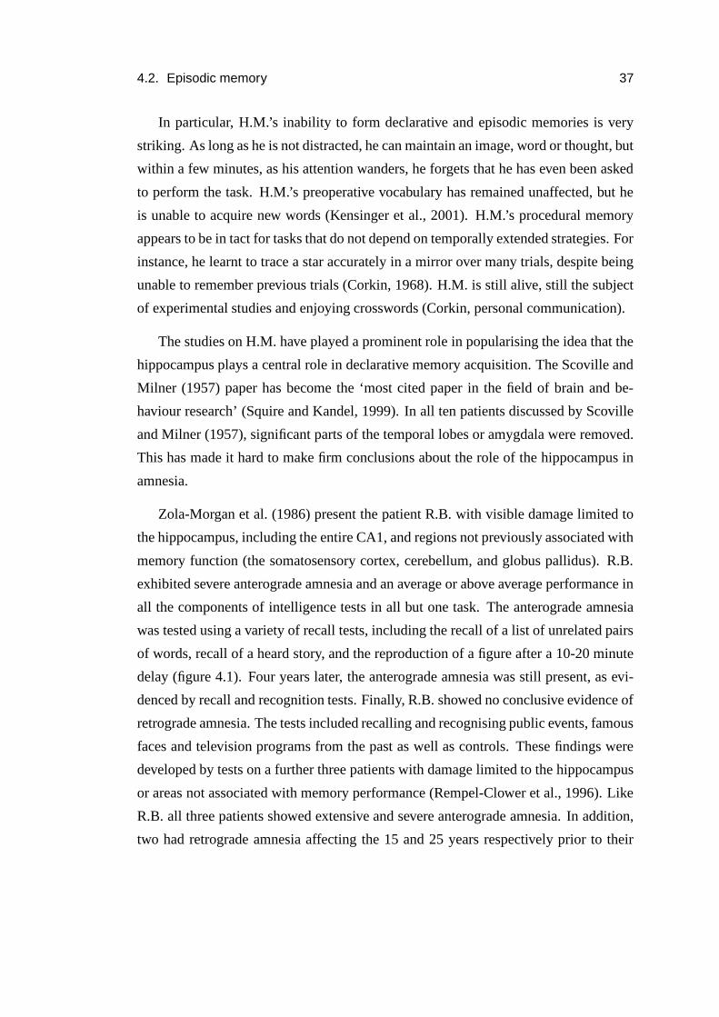
Zola-Morgan et al. (1986) present the patient R.B. with visible damage limited to
the hippocampus, including the entire CA1, and regions not previously associated with
memory function (the somatosensory cortex, cerebellum, and globus pallidus). R.B.
exhibited severe anterograde amnesia and an average or above average performance in
all the components of intelligence tests in all but one task. The anterograde amnesia
was tested using a variety of recall tests, including the recall of a list of unrelated pairs
of words, recall of a heard story, and the reproduction of a figure after a 10-20 minute
delay (figure 4.1). Four years later, the anterograde amnesia was still present, as evi-
denced by recall and recognition tests. Finally, R.B. showed no conclusive evidence of
retrograde amnesia. The tests included recalling and recognising public events, famous
faces and television programs from the past as well as controls. These findings were
developed by tests on a further three patients with damage limited to the hippocampus
or areas not associated with memory performance (Rempel-Clower et al., 1996). Like
R.B. all three patients showed extensive and severe anterograde amnesia. In addition,
two had retrograde amnesia affecting the 15 and 25 years respectively prior to their
38 Chapter 4. Behaviour
Figure 4.1: The performance of patient R.B. and a control in the Rey-Osterreith complex figure test.
The original figure is shown in the small box (bottom left).Subjects are asked to copy the figure (top),
and then asked to reproduce it unseen 10-20 minutes later, without warning (bottom). Left : R.B.’s per-
formance 6 months after the onset of amnesia. Middle: R.B.’s performance 23 months after the amnesia
onset. Right : performance by a control matched for age and education. Figure taken from Zola-Morgan
et al. (1986), c�
Society for Neuroscience.
injuries.
Amnesia is a medically defined condition with diverse pathologies. For instance,
chronic alcohol abuse can lead to an amnesia resulting from damage to regions includ-
ing the thalamus, hypothalamus, mamillary bodies (and not primarily the hippocam-
pus), a condition known as Korsakoff’s syndrome (McEntee and Mair, 1990). The
problem of identifying the contribution of hippocampal damage to amnesia can be
simplified by attempting instead to identify its role in a framework of memory pro-
cesses. The high level taxonomies of memory systems are widely agreed upon, for
instance the distinction between declarative and procedural memory, although differ-
ent researchers have favoured taxonomies. Declarative memories are the facts and data
acquired from experiences, whereas procedural memories are the adjustments to the
neural systems generating these experiences (Cohen and Eichenbaum, 1993, chapter
3).
More controversially, Tulving (1972) has proposed that declarative memory is di-
4.2. Episodic memory 39
visible into semantic and episodic memory. As originally proposed, episodic memories
are the memories of personally experienced events, the memories of what happened,
where and when, whereas semantic memories are knowledge independent of spatial
and temporal contexts. The idea of episodic memory has since been developed to em-
brace the conscious awareness of an event either remembered from the past or planned
in the future (Tulving, 2001). This distinction is useful in humans to distinguish be-
tween strategies used to perform recognition memory tasks: if recall is used to perform
a recognition task, the subject will be aware of it.
Associative memory models of the hippocampus have, since Marr (1971), pro-
posed that sensory and internally generated experiences result in an hippocampal input
which is associated together on a fast time scale, for the future reference of the an-
imal to that experienced event (chapter 5). The specific details are diverse, with the
input activity either referencing or representing sensory and internally generated brain
activity (Teyler and DiScenna, 1986), and the rapidly acquired memory either being
consolidated outside the hippocampus or maintained permanently in the hippocampus
(Alvarez and Squire, 1994; Nadel and Moscovitch, 1997). This function corresponds
most closely to the idea of episodic memory.
The idea that the hippocampus performs episodic memory function is contested.
For instance, Cohen and Eichenbaum (1993) develop a compelling case that the hip-
pocampus has a ‘critical role’ in the acquisition of declarative memories, and that this
is not contained by the idea of the hippocampus as an episodic memory store. This
view has been subsequently developed, particularly focussing on how the hippocampus
forms linked episodic representations that together form a memory space supporting
inference (Eichenbaum, 2001).
Within the still hotly contested debate as to the exact function of the hippocampus
in the declarative memory system, the implications of each theory have only limited
consequences for associative memory models of the hippocampus. I will take the view
that the hippocampus performs the least computations consistent with experimental
data. For instance, the hippocampus may form flexible, relational representations, as
argued by Cohen and Eichenbaum (1993), but it may perform this by associating the
appropriate, as yet unspecified inputs that provide this structure to the memory. This
40 Chapter 4. Behaviour
is in contrast to the hippocampus computing the structure of the relationships between
the inputs itself. As an example, the parietal cortex is preferentially active when infor-
mation is available to disambiguate the relationships between multiple visual objects
(Shafritz et al., 2002). As another example, a common function argued for the hip-
pocampus is that it detects novel stimuli, or combinations of stimuli (Vinogradova,
2001, reviewing a lifetime’s work). Recognition memory is supported by extrahip-
pocampal regions (Brown and Aggleton, 2001), and the encoding of novel stimuli as
an episode is indistinguishable from detecting the novel stimulus. Therefore the default
assumption in this thesis is that hippocampal activity can assist in many memory tasks
by providing recalled episodes, but that the hippocampus itself does not extrapolate
further information from them.
A fundamental criticism of the position that the hippocampus operates as an asso-
ciative memory store is the rejection of the idea of multiple memory systems. Gaffan
(2002) argues that the memory deficits attributed to medial temporal lobe damage,
as exemplified by H.M., are equally consistent with the effects of disconnecting the
temporal cortex from brainstem and basal forebrain afferents. These fibre bundles are
connected to the temporal lobes in the fornix and next to the amygdala. They are
therefore likely to be damaged in H.M.. It is unlikely that this argument can be used
to explain the deficits exhibited by patients such as R.B., whose damage appears to be
restricted to the hippocampus.
4.2.1 Episodic-like memory in animals
If the hippocampus is responsible for episodic memory storage in humans, can this the-
ory be tested in animal models? There are numerous problems to this approach. The
first is the refined definition of episodic memory to include conscious awareness of the
recalled memory. If animals lack consciousness, then by construction animals cannot
have episodic memory. The importance of conscious awareness is to distinguish be-
tween familiarity recognition and recall. Computationally, the representation used in
recall will be a reduced representation of the original event experience, and the repre-
sentation used to judge familiarity can be viewed as a highly reduced representation
of this experience, reduced to a binary variable. If a task can be solved that cannot be
4.2. Episodic memory 41
solved using familiarity alone, and the task requires the hippocampus, then evidence
for an equivalent hippocampal function in our animal is achieved. Because any such
task only tests a restricted part of the definition of episodic memory it is referred to as
‘episodic-like’ memory (Clayton and Dickinson, 1998).
A more serious problem is whether the hippocampus performs the same or similar
functions in different species. The anatomical organisation is similar between the rat,
primates and humans, although the ratio of the numbers of cells in every area signif-
icantly changes (Rosene and Van Hoesen, 1987). Meanwhile, the invasive nature of
electrophysiological recordings in rats and primates can rarely be performed in hu-
mans. For example, the nature of the θ-rhythm in humans is only just beginning to be
explored, and its behavioural correspondence to the rodent θ-rhythm remains uncon-
firmed (Kahana et al., 2001).
The apparent role of the hippocampus in the human amnesia literature has trig-
gered a large body of experimental work searching for a hippocampal dependence of
an episodic-like memory for animals. Ultimately these findings will not directly trans-
fer between animals. The limited success of these experiments, some of which are dis-
cussed below, present compelling evidence for the kind of one-shot learning memory
systems well served by associative memory models. The ultimate focus of this thesis
is on identifying the role of CA1 in the rat, and how it performs its computations. It is
believed that this is interesting in its own right. In addition, our understanding of the
human hippocampus may be increased through understanding a parallel, similar but
different system.
The most successful experiments in examining the existence and nature of episodic-
like memory in animals have adapted the food caching behaviour of particular bird
species. Clayton and Dickinson (1998) presented scrub jays (Aphelocoma coerulescens)
with either wax worms or peanuts for 15 minutes, and allowed them to cache each food
type in the sand wells of different, visually distinctive food trays. The trays were then
removed and returned either 4 or 124 hours later. After the 4 hour delay, fresh wax
worms were placed in the wells where the wax worms had been cached, but after the
124 hour delay, decayed worms were placed in them. This pre-training was designed
to teach the scrub jays that the wax worms, their preferred food, decayed after 4 hours.
42 Chapter 4. Behaviour
During the test experiments, the birds were allowed to cache one food type in one half
of a tray, then to cache the other food type 120 hours later in the other half of the tray.
After a further delay of 4 hours, the scrub jays were allowed to feed from the tray.
When the peanuts were cached first, the scrub jays maintained their preference for wax
worms by preferring to search the side of the tray where the wax worms had been
stored. When the wax worms were cached first, the scrub jays preferred to search the
peanut side of the tray. This is consistent with the birds knowing the three components
of episodic memory: what they searched for depended on when the food was cached,
and they knew where to look.
The results of Clayton and Dickinson (1998) are the only convincing demonstration
of an animal being able to correctly perform a task on the basis of the temporal, spatial
and identity information after one learning trial. The encoding is binary: peanut vs wax
worm, left vs right, and 4 hours vs 124 hours ago. A highly reduced representation of
the event is therefore sufficient to perform the task. Clayton et al. (2003) examined
the temporal component in a little more detail by varying the interval after which the
birds were tested. In this experiment, the scrub jays learnt during training that cached
crickets were fresh after 1 day, but had decayed by 4 four days. When tested at in-
termediate intervals of 2 or 3 days after caching, the scrub jays searched the side of
the tray with cached crickets, rather than the side with cached peanuts. On the fourth
day, their preference switched to peanuts. The scrub jays’ learnt response to 4 day
old crickets can therefore be discriminated to an accuracy of 1 day from 4, indicating
some temporal specificity. In addition, it indicates that the performance in Clayton and
Dickinson (1998) is unlikely to be explained by differential forgetting rates triggered
by a learnt uncertainty in the wax worm longevity, as this would predict a gradual shift
in preference from crickets to peanuts over the 4 days.
In the rodent literature, the search for episodic-like memory storage has focussed
on one-trial learning. In particular, the focus is on one-trial learning in which changes
in behaviour as a result of the recall of an event can be distinguished from changes in
behaviour simply because a prior event has happened (Morris, 2001). For instance, poi-
son aversion can be learnt within one trial, but the subsequent recognition and avoid-
ance of the poison does not require recall.
4.2. Episodic memory 43
One class of tasks that has proved illuminating is paired associate learning. Exper-
iments have been designed that pair what and where information (Day et al., 2003),
what and when information (Fortin et al., 2002), and where and when information
(Kesner and Novak, 1982). Both Fortin et al. (2002) and Kesner and Novak (1982)
will be discussed later in relation to evidence that the hippocampus is involved in se-
quence learning. In the paradigm developed by Day et al. (2003), the rat has only one
trial to find a scented food pellet in one of 49 sand wells, before returning home. The
rat has a second trial 2 minutes later in which to find a differently scented pellet in a
different well. In the test trial, the rat is given a recall cue in the start box of a small
pellet of one of the trial scents. When the start box is opened, there is a pellet corre-
sponding to the recall cue scent in the same position as in the trial. The rats rapidly
learnt the task within days, as judged by the time spent digging at correct and incorrect
sandwells. When the hippocampi were infused with the NMDAR antagonist D-AP5
15 minutes before the sample trials, performance was at chance levels. When infused
in the 20 minutes between the second sample trial and the test trial, the performance
was not significantly affected.
The results of Day et al. (2003) show that NMDAR-dependent plasticity is required
for a task that appears to require the recall of a single odour-location pairing event. It is
difficult to explain how this task could be performed without some form of event mem-
ory recall. There is no requirement to recall the temporal component of every trial, so
the task cannot demonstrate episodic-like memory. The stimuli are more finely grained
than the binary coding required by the task in Clayton and Dickinson (1998). Day et al.
(2003) do not disaggregate the performance in terms of the spatial distances between
the choice sand wells, but it would indicate the accuracy of the spatial component. If
the rats can distinguish neighbouring sand wells, this would indicate a considerable
level of detail in the memory.
One caveat is that paired associate learning has been argued to require a spatial
(where) component. Gilbert and Kesner (2002) tested the ability of rats to learn paired
associations between a visual object and a location, an odour and a location, and be-
tween a visual object and an odour. Rats with hippocampal lesions were unable to
learn the object-location and odour-location pairings, but were able to learn the object-
44 Chapter 4. Behaviour
odour pairing. If the hippocampus is only involved in generating the spatial map of
the environment, as proposed by O’Keefe and Nadel (1978), then the dependence of
the hippocampus is only a result of the hippocampus cognitive map being unavailable.
That the performance in Day et al. (2003) was unaffected by D-AP5 infusions after
the sample trials, suggests that the presence of the spatial component in the one-trial
pair associations is not sufficient to explain the hippocampal dependence, despite the
spatial components of Fortin et al. (2002) and Kesner and Novak (1982).
The one-trial paired associate paradigm was developed by Day et al. (2003) in
response to criticism of previous work investigating episodic-like memory using the
delayed match to place task investigated by Steele and Morris (1999). In these exper-
iments, the rats were given 4 trials per day to find the location of a hidden platform in
a water maze, from different start locations. The platform location was held constant
every day, and moved between one of 9 locations between days. The rats learn the task
sufficiently quickly that after 5 days of pretraining, there is no performance difference
between the second, third and fourth trial escape latencies: after the first trial the rat
is escaping as quickly as it can. When rats were given hippocampal injections of D-
AP5, the escape latency in the second trial was significantly longer, when the interval
between the first and second trial was 20 minutes or more.
This result can be explained by the NMDAR-dependent storage of the first trial
event and subsequent recall in the second trial. It could also be explained by famil-
iarity: the rat swims towards the most familiar location. Despite this shortcoming, the
paradigm was used by Nakazawa et al. (2003) to test the speed of learning in mice with
NMDA NR1 receptor subunit gene knocked out in CA3 pyramidal cells. The escape
latency of the knockout mice in the second trial was significantly longer, despite com-
parable performance during training. The hippocampal NMDAR-dependence of the
task may then be further identified with plasticity in CA3 specifically.
4.2.2 Temporal order
Inspired by studies on the performance of human amnesiacs in temporal order tasks,
Kesner and Novak (1982) investigated the ability of rats with hippocampal lesions to
perform a primacy task. The rats were trained to explore the arms of an eight-arm maze
4.2. Episodic memory 45
in a controlled random order, and then, after a 20 second delay, to choose the arm they
had visited first from a test pair. Control rats performed well in choices between the
earliest arms visited, and between the most recently visited. Lesioned rats performed
as well as controls in the choices between recently visited arms, but at chance levels
for the first visited. When the delay was extended to ten minutes, controls performed
at chance levels except for choices between the most recently visited arms. The le-
sioned rats performed at chance levels for all choices. These results are consistent with
the literature on some amnesiacs with hippocampal damage, where performance in re-
cency discrimination tasks without delays is relatively unimpaired, despite significant
impairment in content discrimination tasks (Sagar et al., 1990).
The experimental design in Kesner and Novak (1982) involved a strong spatial
component which could explain the hippocampal dependence. Fortin et al. (2002)
trained rats to dig in sandwells with odours mixed in, and then discriminate the earliest
occurring odour of a pair from the sequence. Each trial occurs in the same location,
implying that the spatial context does not need to be remembered to perform the task
successfully. Consistent with the results of Kesner and Novak (1982), hippocampus
lesioned rats performed significantly less well than controls.
The experiment of Fortin et al. (2002) shows that the hippocampus is required to
correctly recollect temporal order information. The results are consistent with the idea
that the hippocampus associates discontiguous events, such that recall of the first event
results in the replay of the whole sequence (Levy, 1989; Wallenstein et al., 1998), as
suggested by Fortin et al. (2002). Alternatively, discriminating the primacy of an event
from a sequence out of a pair of events could require recalling the memories of the
unlinked choice events from the hippocampus.
4.2.2.1 CA1 and temporal order
Gilbert et al. (2001) trained CA1 lesioned and control rats to explore all eight arms of
an eight-arm maze in a predetermined random order, and then choose the arm visited
the earliest out of a choice of two. The CA1 lesioned rats were significantly impaired,
performing only marginally better than at chance levels. Spatial recognition was also
assessed, using a delayed matching to sample task. Random objects marked vari-
46 Chapter 4. Behaviour
ously spaced choice foodwells in a circular environment with multiple foodwells, and
the rats were trained to return to a baited foodwell when returned after a delay. The
CA1 lesioned rats’ performance showed no evidence of their impairment. In contrast,
dentate gyrus lesioned rats were highly impaired. For the largest choice separation dis-
tances � 60 cm, the increase in errors was not significant, but as the distance decreased
the significance increased. For separations of 15 cm, the dentate gyrus lesioned rats
performed little above chance. At this distance, the CA1 lesioned rats performed sig-
nificantly worse than the controls, but still within the criteria of successful pretraining.
Gilbert et al. (2001) claim that CA1 in particular is required for temporal order
tasks. They propose that CA1 temporally decorrelates CA3 representation. The only
anatomically distinguished projections from CA3 are to CA1 and the lateral septum
(Amaral and Witter, 1995). If CA1 is completely removed, then hippocampal output
can only be mediated through the lateral septum, presumably to the medial septum
which heavily projects to the subiculum. This is possible, given the existence of spatial
information in the lateral septum (Bezzi et al., 2002), but the lack of spatial activity in
the medial septum makes this theory highly speculative.
CA1 was not completely removed. 17% of ventral CA1 remained by volumetric
analysis. Moser et al. (1995) examined how the size of a dorsal or ventral lesion
affected the ability to acquire a spatial recognition water maze task. With only 20-
40% of dorsal hippocampus, the speed of acquisition was not affected. With only 20-
40% of ventral hippocampus, the task acquisition was severely disrupted. The broad
place fields in the ventral hippocampus (Jung et al., 1994) indicate that the dorsal
hippocampus is more involved in spatial learning, as supported, but dorsally lesioned
animals can still learn the task if trained appropriately (de Hoz et al., 2003). The
extensive postoperative testing in Gilbert et al. (2001), consisting of 2 blocks of 80
trials over 2 weeks, are unusual and could have allowed the rats to acquire the task
given their prior training.
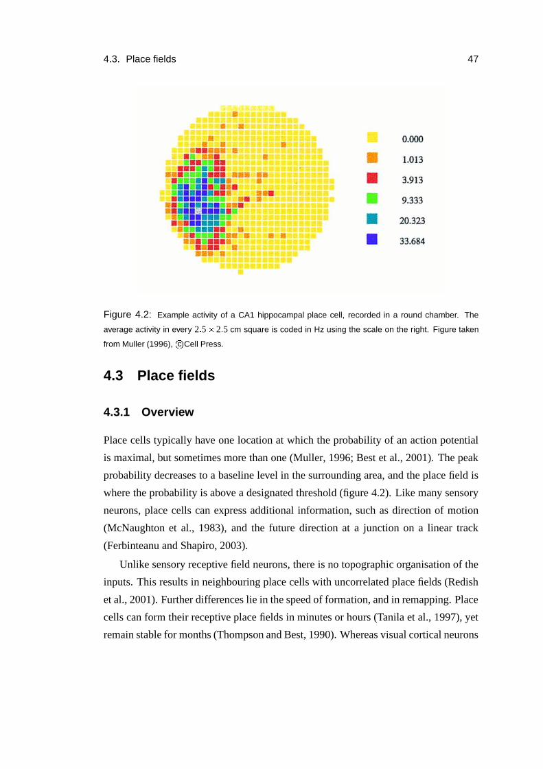
4.3. Place fields 47
Figure 4.2: Example activity of a CA1 hippocampal place cell, recorded in a round chamber. The
average activity in every 2 � 5 � 2 � 5 cm square is coded in Hz using the scale on the right. Figure taken
from Muller (1996), c�
Cell Press.
4.3 Place fields
4.3.1 Overview
Place cells typically have one location at which the probability of an action potential
is maximal, but sometimes more than one (Muller, 1996; Best et al., 2001). The peak
probability decreases to a baseline level in the surrounding area, and the place field is
where the probability is above a designated threshold (figure 4.2). Like many sensory
neurons, place cells can express additional information, such as direction of motion
(McNaughton et al., 1983), and the future direction at a junction on a linear track
(Ferbinteanu and Shapiro, 2003).
Unlike sensory receptive field neurons, there is no topographic organisation of the
inputs. This results in neighbouring place cells with uncorrelated place fields (Redish
et al., 2001). Further differences lie in the speed of formation, and in remapping. Place
cells can form their receptive place fields in minutes or hours (Tanila et al., 1997), yet
remain stable for months (Thompson and Best, 1990). Whereas visual cortical neurons
48 Chapter 4. Behaviour
adapt over days to changes in stimuli, after a behaviourally significant change in the
environment place cells appear to randomly remap their place field location (Bostock
et al., 1991).
The discovery of place cells was a surprising example of an internal representation
of the external environment (O’Keefe and Dostrovsky, 1971). Places fields are located
in an allocentric (world-centred) coordinate system defined by cues in the environment.
O’Keefe and Nadel (1978) specified this internal representation as the ‘cognitive map’
by which the rat could perform spatial navigation. In the ‘strong interpretation’ of the
cognitive map theory the hippocampus only computes the animals’ location within a
representation of the environment (O’Keefe, 1999), and navigation decisions are made
extrahippocampally on the basis of this information. In ‘softer’ interpretations, further
computations are performed by the hippocampus, such as the addition of a temporal
component to form temporal spatial memories.
Place cells are found throughout the hippocampus (Barnes et al., 1990). The most
spatially specific are found in dentate gyrus granule cells (Jung and McNaughton,
1993) and dorsal CA3 and CA1. Place fields in the ventral hippocampus are larger
(Jung et al., 1994). CA3 and CA1 interneurons convey some, but relatively little spatial
information (Kubie et al., 1990). Most of the cortical areas that receive hippocampal
outputs exhibit significant place field activity, including the subiculum, parasubicu-
lum, perirhinal cortex and the deep layers of the entorhinal cortex (Barnes et al., 1990;
Taube, 1995; Burwell et al., 1998; Frank et al., 2001). The lateral septum is an out-
put area as it receives input from the entorhinal cortex, CA3, CA1 and subiculum, but
only weakly projects back to the hippocampus (Jakab and Leranth, 1995). It has re-
cently been shown to exhibit place specific activity, in contrast with the reciprocally
connected medial septum, whose activity appears to correlate with the generation of
hippocampal rhythms (Zhou et al., 1999; Leutgeb and Mizumori, 2002). The medial
prefrontal cortex receives a projection from CA1 but so far there have been no reports
of prefrontal place field activity (Poucet, 1997).
4.3. Place fields 49
4.3.2 Activity in novel environments
When a rat is placed in a novel environment, the average CA1 pyramidal cell rate in-
creases (Wilson and McNaughton, 1993) by 43% over an initial period of 10-20 min-
utes (Nitz and McNaughton, 2004). Within 2-3 minutes place field activity occurs, and
after about 10 minutes, stable place fields are observed (Bostock et al., 1991; Wilson
and McNaughton, 1993). At the same time, CA1 interneuron activity decreases (Wil-
son and McNaughton, 1993; Fyhn et al., 2002): by 16.6�
6.5% over 33 interneurons
from all layers (Nitz and McNaughton, 2004).
If the now familiar environment is sufficiently adjusted, the place fields ‘remap’
(Bostock et al., 1991) as though the environment is novel. Environmental changes that
can elicit remapping include the removal, introduction or relocation of behaviourally
relevant objects. The behavioural relevance of environmental manipulations is very
important. If a landmark cue is added to an arena once the spatial location of the
goal has been learnt with respect to existing landmark cues, rats perform at chance
levels when only the new landmark cue is used in tests (Biegler and Morris, 1999).
Alternatively, if the visual cues are consistent with two different orientations of a four
arm maze, then the place field map is consistent with one of these options, and the
rats will search in the goal location consistent with this map (O’Keefe and Speakman,
1987).
Particular manipulations of the environment often result in partial remappings,
where the place fields of only a subset of cells change. These include introducing
a barrier, or changing the proportions of the arena (Muller and Kubie, 1987; O’Keefe
and Burgess, 1996). When the location of a behaviourally relevant object is changed
in a familiar environment, activity similar to a partial remap is observed. Fyhn et al.
(2002) trained rats in the water maze task, then in test trials recorded the activity when
the hidden platform location was changed. In the new platform location, the activity
of a subset of interneurons decreased. Previously silent pyramidal cells became highly
active, but their activity levels decayed over ‘tens of seconds’. In subsequent trials,
when the new platform location is maintained, place field centres at other locations
were not significantly changed. This activity is consistent with ‘misplace’ cells de-
scribed by O’Keefe and Nadel (1978); cells whose activity is spatially modulated, but
50 Chapter 4. Behaviour
whose rate is maximal when unexpected objects or goals are found, or expected objects
or goals are not found.
NMDAR manipulations demonstrate a role of NMDAR-mediated plasticity in the
successful initial formation of place fields. Mice lacking the NMDA NR1 receptor
subunit in CA1 show no significant LTP in the Schaffer collaterals in the slice, and are
unable to learn the Morris hidden platform water maze task (Tsien et al., 1996). De-
spite this, their place fields are only � 30% larger, a result possibly explained by home-
ostatic mechanisms adjusting the threshold of every CA1 pyramidal cell (McHugh
et al., 1996). Place fields can form in the presence of NMDA antagonists, but when the
lights are turned off for five minutes and then turned back on, the fields remap (Shapiro
and Eichenbaum, 1999).
Meanwhile, Nakazawa et al. (2003) examined place field formation in mice with
the NMDA NR1 receptor subunit gene knocked out in CA3 pyramidal cells. The mice
were familiarised with a linear track by running back and forth for 15 minutes, and
CA1 place field activity was recorded for 15 minutes the next day. Both the mutant
and control mice had statistically inseparable firing rates and field sizes. A partition
was then removed at one end of the track to reveal another linear track, and the mice
explored it. Over the first 15 minutes in this linear track, the place field sizes of the
mutant mice increased by � 50%, where the place field sizes of control mice remained
unchanged. By the next day, the mutant place field sizes had returned to the size of
the control place fields. Nakazawa et al. (2003) state that the larger place field sizes on
entering a novel environment is consistent with CA1 cells being principally driven by
temporoammonic input. This is illogical: if temporoammonic input predominates dur-
ing place field formation, then this will reduce the effect of differences in CA3 between
mutants and controls. More plausibly, the mutant CA1 place fields are larger because
their CA3 place fields are larger, but the influence of Schaffer collateral plasticity and
temporoammonic input compensate for this over one day.
The Schaffer collaterals are highly plastic during the early excitatory CA1 activity
in response to spatial novelty. Weak stimulation (at 0.033 Hz) does not produce signifi-
cant LTP in the stationary rat in a familiar environment, but produces significant LTP 5
minutes after the rat had returned from 5 minutes of exploring a novel environment (Li
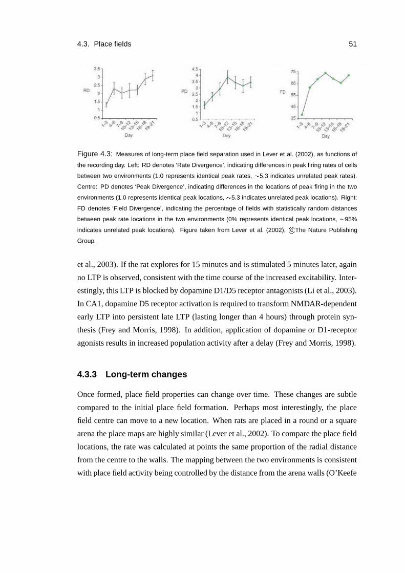
4.3. Place fields 51
Figure 4.3: Measures of long-term place field separation used in Lever et al. (2002), as functions of
the recording day. Left: RD denotes ‘Rate Divergence’, indicating differences in peak firing rates of cells
between two environments (1.0 represents identical peak rates, � 5.3 indicates unrelated peak rates).
Centre: PD denotes ‘Peak Divergence’, indicating differences in the locations of peak firing in the two
environments (1.0 represents identical peak locations, � 5.3 indicates unrelated peak locations). Right:
FD denotes ‘Field Divergence’, indicating the percentage of fields with statistically random distances
between peak rate locations in the two environments (0% represents identical peak locations, � 95%
indicates unrelated peak locations). Figure taken from Lever et al. (2002), c�
The Nature Publishing
Group.
et al., 2003). If the rat explores for 15 minutes and is stimulated 5 minutes later, again
no LTP is observed, consistent with the time course of the increased excitability. Inter-
estingly, this LTP is blocked by dopamine D1/D5 receptor antagonists (Li et al., 2003).
In CA1, dopamine D5 receptor activation is required to transform NMDAR-dependent
early LTP into persistent late LTP (lasting longer than 4 hours) through protein syn-
thesis (Frey and Morris, 1998). In addition, application of dopamine or D1-receptor
agonists results in increased population activity after a delay (Frey and Morris, 1998).
4.3.3 Long-term changes
Once formed, place field properties can change over time. These changes are subtle
compared to the initial place field formation. Perhaps most interestingly, the place
field centre can move to a new location. When rats are placed in a round or a square
arena the place maps are highly similar (Lever et al., 2002). To compare the place field
locations, the rate was calculated at points the same proportion of the radial distance
from the centre to the walls. The mapping between the two environments is consistent
with place field activity being controlled by the distance from the arena walls (O’Keefe
52 Chapter 4. Behaviour
and Burgess, 1996). With repeated sessions, the similarities of the place field maps in
the two arenas significantly diverge: individual fields either gradually move, disappear,
or develop a subfield which comes to predominate (figure 4.3).
The actual shape of the place field also changes. If the rat runs in one direction
along a linear track, the place fields become asymmetric such that the rate is low as the
rat enters the field, and high in the latter part of the field (Mehta et al., 2000). At the
same time, the fields increased by � 20% in width and the place field centres moved� 2.5 cm in the direction opposite to the direction of motion (Mehta et al., 2000, 1997).
Place fields formed with NMDARs blocked are initially stable over hours, but when
the rat returns to the environment the next day, a new map is established (Kentros et al.,
1998). The long-term stability of place fields is equivalently blocked by anisomycin,
an inhibitor of the protein synthesis triggered by NMDA plasticity (Agnihotri et al.,
2004). The asymmetric place field expansion is also prevented by NMDA blockers
(Ekstrom et al., 2001). NMDA mediated spike time-dependent plasticity has been
observed in the Schaffer collaterals in vitro (Nishiyama et al., 2000), consistent with
the theoretical models of sequence learning in CA3 that predicted the phenomenon
(Levy, 1989; Abbott and Blum, 1996; Tsodyks et al., 1996).
4.3.4 Spatially correlated activity in the entorhinal cortex
If place fields are generated in the hippocampus, what information are they generated
from? Barnes et al. (1990) were the first to record the spatial correlates of entorhi-
nal activity. They made recordings of entorhinal, hippocampal and subicular neurons
while the rat performed a task in an eight-arm maze. The spatial correlate of the activ-
ity was quantified as the ‘specificity’, the mean activity along an arm with the highest
mean activity divided by the mean activity elsewhere. The specificity of the entorhinal
cells is approximately equal to that of CA1 interneurons. The authors point out that
this measure does not identify spatially consistent firing in multiple locations.
Quirk et al. (1992) were interested in identifying whether or not remapping is a re-
sult of changes upstream from the hippocampus. They found that the ‘patchiness’ (the
number of continuous regions of high rate activity) of entorhinal cells is highly cor-
related between the two environments, whereas the patchiness of hippocampal cells
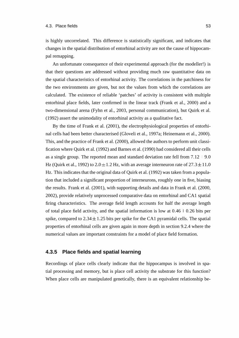
4.3. Place fields 53
is highly uncorrelated. This difference is statistically significant, and indicates that
changes in the spatial distribution of entorhinal activity are not the cause of hippocam-
pal remapping.
An unfortunate consequence of their experimental approach (for the modeller!) is
that their questions are addressed without providing much raw quantitative data on
the spatial characteristics of entorhinal activity. The correlations in the patchiness for
the two environments are given, but not the values from which the correlations are
calculated. The existence of reliable ‘patches’ of activity is consistent with multiple
entorhinal place fields, later confirmed in the linear track (Frank et al., 2000) and a
two-dimensional arena (Fyhn et al., 2003, personal communication), but Quirk et al.
(1992) assert the unimodality of entorhinal activity as a qualitative fact.
By the time of Frank et al. (2001), the electrophysiological properties of entorhi-
nal cells had been better characterised (Gloveli et al., 1997a; Heinemann et al., 2000).
This, and the practice of Frank et al. (2000), allowed the authors to perform unit classi-
fication where Quirk et al. (1992) and Barnes et al. (1990) had considered all their cells
as a single group. The reported mean and standard deviation rate fell from 7 � 12�
9 � 0
Hz (Quirk et al., 1992) to 2 � 0�
1 � 2 Hz, with an average interneuron rate of 27 � 3�
11 � 0
Hz. This indicates that the original data of Quirk et al. (1992) was taken from a popula-
tion that included a significant proportion of interneurons, roughly one in five, biasing
the results. Frank et al. (2001), with supporting details and data in Frank et al. (2000,
2002), provide relatively unprocessed comparative data on entorhinal and CA1 spatial
firing characteristics. The average field length accounts for half the average length
of total place field activity, and the spatial information is low at 0 � 46�
0 � 26 bits per
spike, compared to 2 � 34�
1 � 25 bits per spike for the CA1 pyramidal cells. The spatial
properties of entorhinal cells are given again in more depth in section 9.2.4 where the
numerical values are important constraints for a model of place field formation.
4.3.5 Place fields and spatial learning
Recordings of place cells clearly indicate that the hippocampus is involved in spa-
tial processing and memory, but is place cell activity the substrate for this function?
When place cells are manipulated genetically, there is an equivalent relationship be-
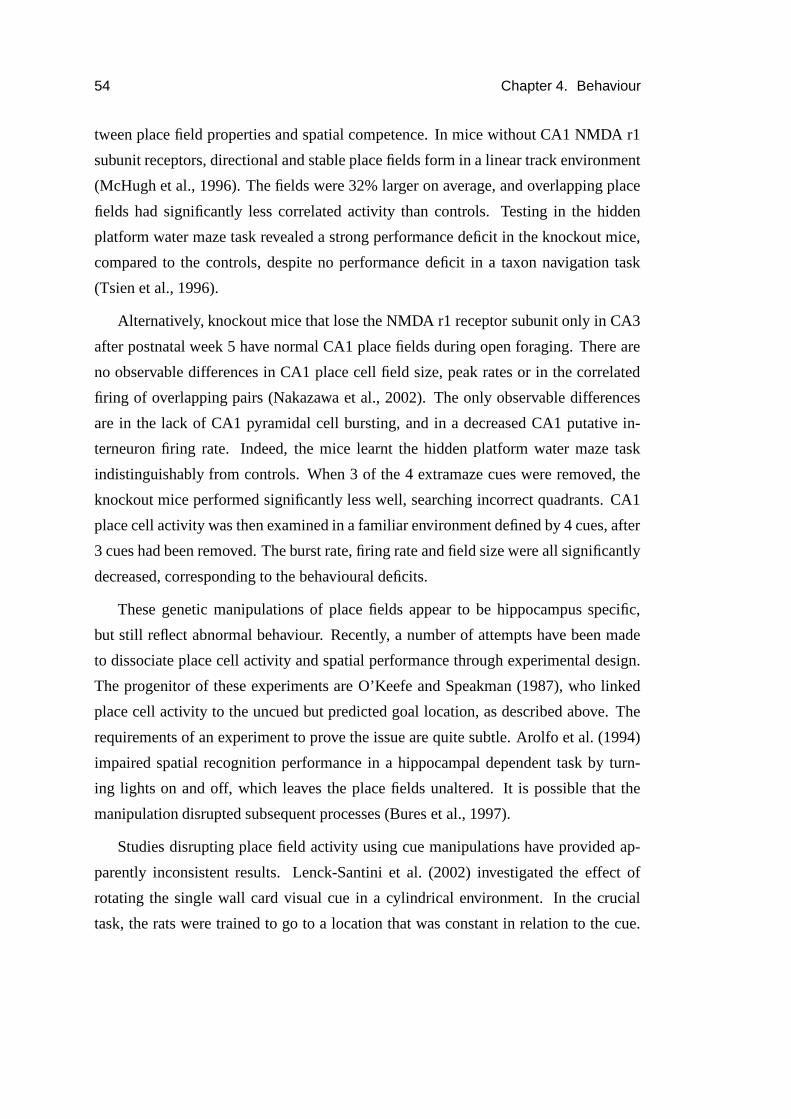
54 Chapter 4. Behaviour
tween place field properties and spatial competence. In mice without CA1 NMDA r1
subunit receptors, directional and stable place fields form in a linear track environment
(McHugh et al., 1996). The fields were 32% larger on average, and overlapping place
fields had significantly less correlated activity than controls. Testing in the hidden
platform water maze task revealed a strong performance deficit in the knockout mice,
compared to the controls, despite no performance deficit in a taxon navigation task
(Tsien et al., 1996).
Alternatively, knockout mice that lose the NMDA r1 receptor subunit only in CA3
after postnatal week 5 have normal CA1 place fields during open foraging. There are
no observable differences in CA1 place cell field size, peak rates or in the correlated
firing of overlapping pairs (Nakazawa et al., 2002). The only observable differences
are in the lack of CA1 pyramidal cell bursting, and in a decreased CA1 putative in-
terneuron firing rate. Indeed, the mice learnt the hidden platform water maze task
indistinguishably from controls. When 3 of the 4 extramaze cues were removed, the
knockout mice performed significantly less well, searching incorrect quadrants. CA1
place cell activity was then examined in a familiar environment defined by 4 cues, after
3 cues had been removed. The burst rate, firing rate and field size were all significantly
decreased, corresponding to the behavioural deficits.
These genetic manipulations of place fields appear to be hippocampus specific,
but still reflect abnormal behaviour. Recently, a number of attempts have been made
to dissociate place cell activity and spatial performance through experimental design.
The progenitor of these experiments are O’Keefe and Speakman (1987), who linked
place cell activity to the uncued but predicted goal location, as described above. The
requirements of an experiment to prove the issue are quite subtle. Arolfo et al. (1994)
impaired spatial recognition performance in a hippocampal dependent task by turn-
ing lights on and off, which leaves the place fields unaltered. It is possible that the
manipulation disrupted subsequent processes (Bures et al., 1997).
Studies disrupting place field activity using cue manipulations have provided ap-
parently inconsistent results. Lenck-Santini et al. (2002) investigated the effect of
rotating the single wall card visual cue in a cylindrical environment. In the crucial
task, the rats were trained to go to a location that was constant in relation to the cue.
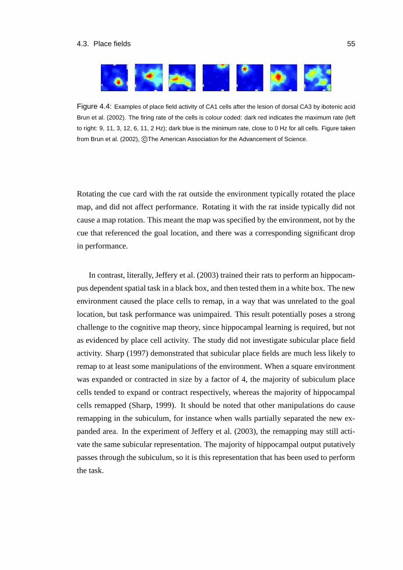
4.3. Place fields 55
Figure 4.4: Examples of place field activity of CA1 cells after the lesion of dorsal CA3 by ibotenic acid
Brun et al. (2002). The firing rate of the cells is colour coded: dark red indicates the maximum rate (left
to right: 9, 11, 3, 12, 6, 11, 2 Hz); dark blue is the minimum rate, close to 0 Hz for all cells. Figure taken
from Brun et al. (2002), c�
The American Association for the Advancement of Science.
Rotating the cue card with the rat outside the environment typically rotated the place
map, and did not affect performance. Rotating it with the rat inside typically did not
cause a map rotation. This meant the map was specified by the environment, not by the
cue that referenced the goal location, and there was a corresponding significant drop
in performance.
In contrast, literally, Jeffery et al. (2003) trained their rats to perform an hippocam-
pus dependent spatial task in a black box, and then tested them in a white box. The new
environment caused the place cells to remap, in a way that was unrelated to the goal
location, but task performance was unimpaired. This result potentially poses a strong
challenge to the cognitive map theory, since hippocampal learning is required, but not
as evidenced by place cell activity. The study did not investigate subicular place field
activity. Sharp (1997) demonstrated that subicular place fields are much less likely to
remap to at least some manipulations of the environment. When a square environment
was expanded or contracted in size by a factor of 4, the majority of subiculum place
cells tended to expand or contract respectively, whereas the majority of hippocampal
cells remapped (Sharp, 1999). It should be noted that other manipulations do cause
remapping in the subiculum, for instance when walls partially separated the new ex-
panded area. In the experiment of Jeffery et al. (2003), the remapping may still acti-
vate the same subicular representation. The majority of hippocampal output putatively
passes through the subiculum, so it is this representation that has been used to perform
the task.
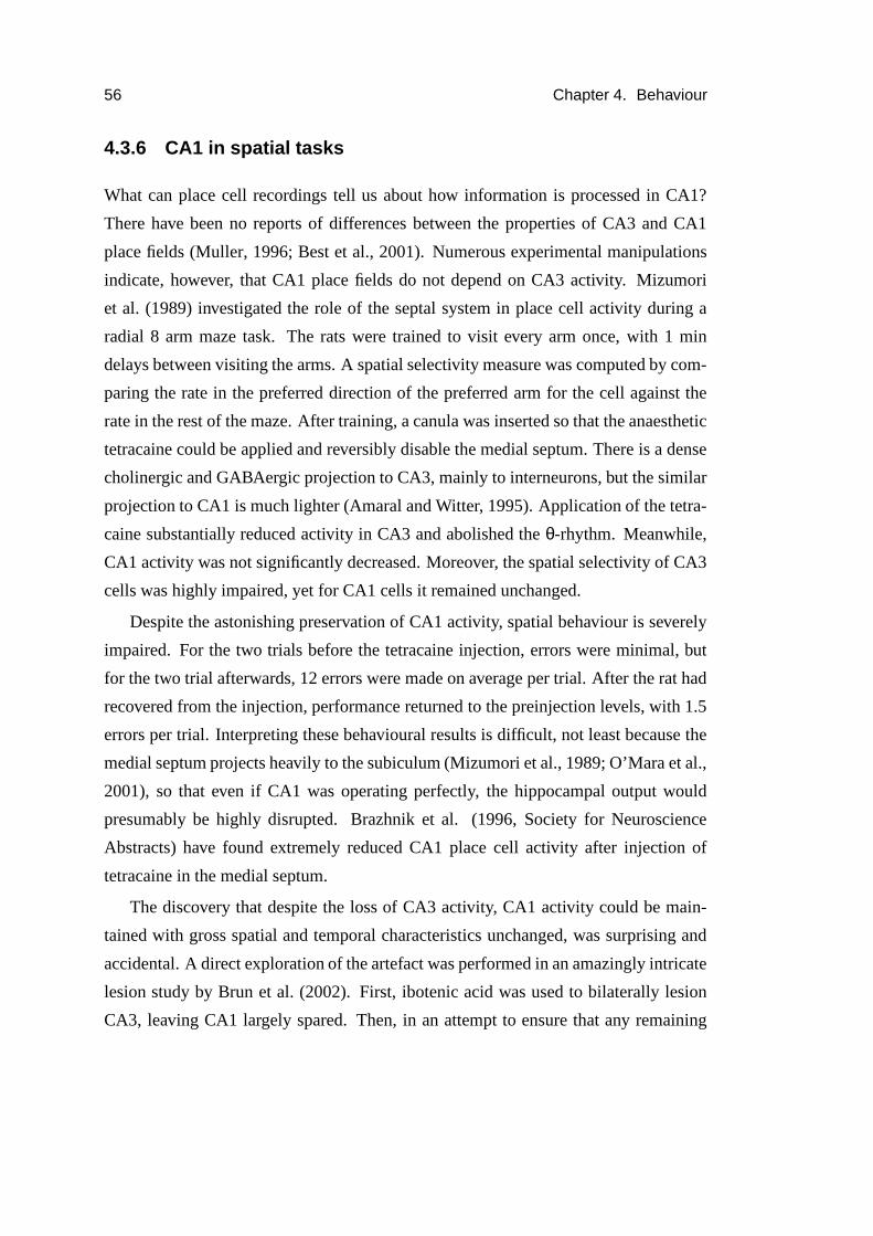
56 Chapter 4. Behaviour
4.3.6 CA1 in spatial tasks
What can place cell recordings tell us about how information is processed in CA1?
There have been no reports of differences between the properties of CA3 and CA1
place fields (Muller, 1996; Best et al., 2001). Numerous experimental manipulations
indicate, however, that CA1 place fields do not depend on CA3 activity. Mizumori
et al. (1989) investigated the role of the septal system in place cell activity during a
radial 8 arm maze task. The rats were trained to visit every arm once, with 1 min
delays between visiting the arms. A spatial selectivity measure was computed by com-
paring the rate in the preferred direction of the preferred arm for the cell against the
rate in the rest of the maze. After training, a canula was inserted so that the anaesthetic
tetracaine could be applied and reversibly disable the medial septum. There is a dense
cholinergic and GABAergic projection to CA3, mainly to interneurons, but the similar
projection to CA1 is much lighter (Amaral and Witter, 1995). Application of the tetra-
caine substantially reduced activity in CA3 and abolished the θ-rhythm. Meanwhile,
CA1 activity was not significantly decreased. Moreover, the spatial selectivity of CA3
cells was highly impaired, yet for CA1 cells it remained unchanged.
Despite the astonishing preservation of CA1 activity, spatial behaviour is severely
impaired. For the two trials before the tetracaine injection, errors were minimal, but
for the two trial afterwards, 12 errors were made on average per trial. After the rat had
recovered from the injection, performance returned to the preinjection levels, with 1.5
errors per trial. Interpreting these behavioural results is difficult, not least because the
medial septum projects heavily to the subiculum (Mizumori et al., 1989; O’Mara et al.,
2001), so that even if CA1 was operating perfectly, the hippocampal output would
presumably be highly disrupted. Brazhnik et al. (1996, Society for Neuroscience
Abstracts) have found extremely reduced CA1 place cell activity after injection of
tetracaine in the medial septum.
The discovery that despite the loss of CA3 activity, CA1 activity could be main-
tained with gross spatial and temporal characteristics unchanged, was surprising and
accidental. A direct exploration of the artefact was performed in an amazingly intricate
lesion study by Brun et al. (2002). First, ibotenic acid was used to bilaterally lesion
CA3, leaving CA1 largely spared. Then, in an attempt to ensure that any remaining
4.3. Place fields 57
CA3 was completely disconnected, the contralateral hippocampus was removed and
cuts were made between CA3 and CA1. Post-operative fluorescent retrograde tracing
identified a small number of neurons still connected at the septal pole. With this le-
sion performed on 11 rats, stable directional place fields and normal θ-activity were
observed. The peak place cell rates were slightly reduced, but overall firing rates were
not significantly different and nor was the average place field size. The sparseness in-
creased, indicating a loss of neurons with the greatest spatial information (Treves and
Rolls, 1991).
The behavioural relevance of the remaining CA1 activity was first tested with a
spatial recognition task (figure 4.4). The rats were trained to find the hidden escape
platform at a constant location in an annular water maze. Rats with full hippocampus
lesions swam significantly less in the target quadrant than those with CA3 lesions, who
in turn performed equivalently to sham lesion controls. In a more demanding task, the
rats had to swim a lap before the platform became available, still hidden. Rats with
CA3 lesions learnt this task much more slowly than controls, during which time their
escape latencies were significantly longer.

Chapter 5
CA1 and models of the hippocampus
5.1 Introduction
This section is intended to be an exhaustive review of models of the hippocampus that
explicitly model CA1, not including articles in press. Numerous researchers have pur-
sued the consequences of a particular viewpoint in series of models. Within each series
of papers by an author, pivotal models of these series have been chosen to exemplify
the approaches, with important developments or changes in viewpoint discussed under
the same banner.
Given the large number of hippocampal models, it is surprising that only a few
specify a role for CA1. Many models are concerned with the role of the hippocampus
in a larger system, with the hippocampus acting as a homogenous network. Notable
systems include the consolidation of cortical memories (Buzsaki, 1989; Alvarez and
Squire, 1994; Murre, 1996; Kali and Dayan, 2004), navigation (Muller and Stead,
1996; Redish and Touretzky, 1998; Foster et al., 2000; Arleo and Gerstner, 2000;
Gaussier et al., 2002; Koene et al., 2003), and conditioning (Gluck and Myers, 1993;
Buhusi and Schmajuk, 1996; Rodriguez and Levy, 2001). These models do not make
any requirement for the differentiation of CA3 and CA1. At the other extreme, there
are numerous models of synaptic integration in CA1 pyramidal cells that make no
claim for their function (Granger et al., 1994; Graham, 2001; Migliore, 2003; Poirazi
et al., 2003). The models concerned with place field formation, discussed in section 6,
59
60 Chapter 5. CA1 and models of the hippocampus
either model CA3 or are uncorrelated with hippocampal anatomy.
All the models reviewed, with the exception of Lorincz and Buzsaki (2000), are
associative memory models. Their primary focus is the potential of CA3 to autoasso-
ciate (Treves and Rolls, 1994; McClelland and Goddard, 1996) or to associate activity
in sequences (Levy et al., 1998; Lisman and Otmakhova, 2001). The role of the tem-
poroammonic pathway is particularly difficult for the models to explain. As an extreme
argument, the suggested functions such as novelty detection and prediction do not ne-
cessitate CA1, as they can be performed just as well in (one of) the receiving layers.
The anatomy of the hippocampus indicates that a particular computation has to be
performed on the output from CA3 before it is disseminated to the rest of the brain.
Treves and Rolls (1994) argue that CA3 activity benefits from being recoded into a
more robust code. McClelland and Goddard (1996) suggest that CA3 and entorhinal
rates are too high for direct association. These arguments necessitate CA1, but not the
temporoammonic input: the claim of McClelland and Goddard (1996) for an invertible
code confounds the superficial and deep layers of the entorhinal cortex.
5.2 Treves and Rolls (1994)
Inspired by Marr (1971), Treves and Rolls developed a detailed associative memory
model of the hippocampus (Rolls, 1989; Treves and Rolls, 1991, 1992, 1994; Treves,
1995). Following McNaughton and Morris (1987), Marr’s hazy hippocampal anatomy
is refined to identify CA3 as the locus of the recurrent collaterals, vital for pattern
completion in associative memory recall. Further, the binary neurons are replaced by
the more physiologically faithful linear threshold neurons.
The parameter dependence of the capacity of a partially connected, recurrent model
of CA3 is calculated using an energy function analysis (Treves and Rolls, 1991). In
keeping with results from binary networks, low activity levels are crucial for large
capacities, and the capacity has an approximately linear relationship with the connec-
tivity. When new inputs are presented to the network, recurrent collateral activity dom-
inates the dynamics and the pattern is not learnt (Treves and Rolls, 1992). Instead, the
idea is invoked that the large and infrequent mossy fibre synapses on CA3 pyramidal
5.2. Treves and Rolls (1994) 61
cell dendrites act as ‘detonator’ synapses (McNaughton and Morris, 1987), providing
comparatively huge excitatory input. This input is strong enough to prevent CA3 ac-
tivity settling into an already learnt attractor state. These strong mossy fibre inputs
are not associated with the CA3 activity during storage because the synapses exhibit
non-associative, presynaptic LTP. In contrast, the perforant path inputs are presumed
to exhibit associative LTP. During recall from partial cues, the perforant path input is
able to recall the complete pattern of CA3 activity by activating neurons and recurrent
collaterals of the corresponding attractor state, whereas the mossy fibre synapses have
little effect. The function of the dentate gyrus in this model is to create orthogonalized
representations of full-sized patterns of entorhinal activity.
The model has been successful in accounting for behaviour, most sensationally in
the requirement of recurrent collateral plasticity for both one-trial spatial learning and
spatial recall from a reduced number of spatial cues (Nakazawa et al., 2003, 2002).
Equally notable has been the dependence of spatial learning on non-inactivated den-
tate gyrus (Lassalle et al., 2000). The model has provided the conceptual framework
for many experiments, partly because it has persevered with the idea of providing
quantitative data. The model is also attractive in its simplicity: it does not attempt
attribute computations to the hippocampus which could be performed elsewhere, such
as novelty detection, path integration or the organisation of temporal order memory.
Like Marr’s model, it shares the conceptual weakness of being inspired by the data on
declarative memory loss in humans and primates, but being most readily testable on
rodents.
The possible functions of CA1 in the model are discussed at length in Treves and
Rolls (1994). They propose that CA1 must ensure efficient information transmission.
More circumspectly, they also suggest that CA1 acts as a competitive network, re-
ducing the redundancy of the CA3 activity (Rolls, 1989). The recurrent inhibition in
CA1 is weak as evidenced by the lack of recurrent collaterals, and the preponderance
of these collaterals to synapse with dendritically distal projecting stratum oriens in-
terneurons (section 2.4), thus CA1 would seem an unlikely candidate for a competitive
network. Finally, it is suggested that the information rich component of the initial en-
torhinal activity can be integrated with the reduced information but completed CA3
62 Chapter 5. CA1 and models of the hippocampus
representation. This idea assumes that CA3 only performs pattern completion. In the
event of recall from a full but noisy pattern of entorhinal activity, it would significantly
reduce information transmission from CA3 to CA1.
Efficient information transmission is envisaged as benefitting from the recoding of
CA3 activity, such that across the larger CA1 population, every CA1 cell conveys less
information, rendering the code more robust to noise and degradation in the subse-
quent journey back to the neocortex. Expansion recoding is only useful if the process
itself does not lose significant amounts of information. This issue is addressed by
Treves (1995), who calculates the parameter dependence of information transmission
between two populations of rate-based linear-threshold neurons representing CA3 and
CA1. The network uses a covariance plasticity rule, and competition is implemented
using a uniform linear threshold. The network has storage and retrieval modes. In the
storage mode, the CA3 rate coded binary (or ternary) patterns propagate to CA1 via
an incomplete, random synaptic weight matrix. The CA3 and CA1 activity are associ-
ated, but the weight changes do not occur until after all the patterns have been learnt.
In retrieval mode, the synaptic weights consist of the time decayed original weight,
the Hebbian term from the storage of the pattern, and a crosstalk talk. An expression
for the average mutual information of the stored and retrieved patterns is calculated
analytically, and evaluated numerically.
The principal result is that the rate of plasticity in the Schaffer collaterals resulting
in the optimal information transmission is very close to the optimal rate of plasticity
in the CA3 recurrent collaterals for storing a given number of patterns in the network
(Treves and Rolls, 1991). This result appears to hold over a wide range of parameters,
and is argued to be quite general; pathological cases are not presented.
The analysis allows the performance of a full-size CA3 and CA1 network to be
evaluated. Unfortunately, the equations are no more transparent than the operation of
the network. The model makes quantitative evaluations of the parameters, which in
principle can be compared to experiment. The correspondence between the rate of
plasticity in a covariance learning rule and the rate of plasticity in experiments is diffi-
cult to establish because the rate of plasticity depends on the protocol used. The result
about the rate of plasticity becomes a qualitative one, although based on quantitative
5.2. Treves and Rolls (1994) 63
principle of maximising the mutual information.
The parameter exploration also argues that reducing the number of CA1 neurons
in CA1 from twice to 1.5 times the number of CA3 neurons reduces the information
transmitted. This is not a controlled comparison, since the number of synapses is
not held constant. From these results, the information advantage of expansion coding
cannot be fully judged. Schultz and Rolls (1999) continue the parameter search of the
same model, and return to this question amongst others. They consider a continuous
range of sizes of CA1 from nearly zero to 3.5 times the size of CA3. They do not
control for the number of synapses and the amount of information simply increases
with the size of CA1, and little can be usefully concluded. Schultz and Rolls (1999)
also find that topographically organising the Schaffer collaterals either has no effect or
decreases the mutual information. The binary rate coding of CA3 activity results in the
maximum information efficiency (Schultz and Rolls, 1999).
The same model is extended by Fulvi-Mari et al. (1999) to include the entorhinal
cortex and the temporoammonic pathway. The temporoammonic input is presumed
to come from the same entorhinal cells as the perforant path input to CA3, and the ef-
fect of the distal location of temporoammonic synapses with the CA1 pyramidal cells is
approximated by reducing the connectivity. The dynamics in CA3 in recall are approx-
imated by adding a noise term to a perfectly recalled pattern, and the temporoammonic
connections are not plastic. The resulting analytical equations are magnitudes of or-
der more complex than in Treves (1995), and solved numerically with acknowledged
difficulty. Increasing the number of temporoammonic inputs increases the mutual in-
formation of the entorhinal and CA1 activity, but a high level of noise is used in CA3,
so this is not surprising. The model is sufficiently complex that a thorough parameter
exploration has not been forthcoming.
A weakness of the approach taken by Treves (1995) is that the validity of the under-
lying assumption is not addressed, that the function of CA1 is to transfer information
from CA3 to CA1. For instance, there is no control, no examination of the conse-
quences for regions downstream of CA1 if it was not there. The parameter dependence
of CA1 in performing the function is spelt out, but there it is difficult to infer how
well CA1 is adapted to perform it. This is especially true when considering the tem-
64 Chapter 5. CA1 and models of the hippocampus
poroammonic input. Treves (1995) states that information transmission and robustly
recoding CA3 activity are not the only functions of CA1, and that this is implied by
the existence of the temporoammonic pathway. When the temporoammonic input is
included, the equations are sufficiently complex to exclude any systematic exploration
of the function of the temporoammonic input. As Treves (2004) puts it, discussing the
role of CA1, the “...simple quantitative advantage of adding one more processing step
does not appear to be a compelling explanation”.
5.3 McClelland and Goddard (1996)
O’Reilly and McClelland (1994) took up the idea in the literature that the dentate
gyrus creates orthogonalised versions of the entorhinal input to CA3 (e.g. Marr, 1971;
McNaughton and Morris, 1987; Treves and Rolls, 1992). They developed an analytical
model of the feedforward connections between the entorhinal cortex, dentate gyrus and
CA3. In this model, every area is composed of implicitly defined binary neurons, and
every layer is partially connected, much in the style of a Marr network. N-winners-
take-all thresholding is implemented using subtractive inhibition, and the synapses
appear to be Brindley synapses in disguise: all the connected synapses have a weight
of 1, except after learning, when they have a weight 1�
Lr, where Lr is the learning
rate.
Using the binary formalism, the conditional probability that an output neuron is
active in two patterns is calculated. This is used to estimate the expected mean output
pattern overlap as a function of the overlap between the input patterns. By comparing
the ratio of the input and output pattern overlaps, the performance of the network in
pattern separation or in pattern completion is assessed over a large set of parameters.
The competing requirements of pattern completion and separation are argued to be the
motivation behind the dual inputs to CA3, reinforcing the point made by Treves and
Rolls (1992).
In the analysis, the input activity is calculated, rather than dendritic sum distribu-
tions. This simplicity gives clear results. By quantifying the performance advantage of
including the dentate gyrus in pattern separation, the model has been influential in pro-
5.3. McClelland and Goddard (1996) 65
moting the idea of the function of the dentate gyrus as orthogonalising the entorhinal
input to CA3.
In the model of O’Reilly and McClelland (1994), the role of CA1 is to overcome
the problem of associating CA3 activity with the original entorhinal activity. Since the
dentate input results in CA3 activity that is decorrelated with the entorhinal activity, the
authors argue that a layer is required to associate the CA3 output with the entorhinal
input in an ‘invertible’ form. They propose that as entorhinal activity is transferred
to CA3 for storage, entorhinal activity also establishes a pattern of activity in CA1.
The existence of CA1 place fields without activity in CA3 (Mizumori et al., 1989) is
cited in support of this idea. The activity in CA3 is then associated with the activity
in CA1. During recall, CA1 activity reactivates the original entorhinal activity, which
is transmitted back to the rest of the neocortex. Reciprocal connections between CA1
and the entorhinal cortex are responsible for the invertible code, and there is no stated
role for plasticity in these pathways.
This idea of invertibility is developed by McClelland and Goddard (1996), who
explore a model in which every CA1 cell returns connections to EC cells which contact
it. This pattern of connectivity is acknowledged as implausible, and various schemes
are mentioned about how it might be achieved in practice. There is no evidence that
activity in the second and third layers of the entorhinal cortex are related, and CA1
projects to the completely different, deep layers of the entorhinal cortex. Even if the
connections can be plausibly arranged, recalled activity evokes activity in a different
set of entorhinal neurons to the entorhinal neurons active during storage. How the
neurons of the deep layers of the entorhinal cortex contact the appropriate cortical
neurons during the reactivation of a memory is a separate, complex issue.
McClelland and Goddard (1996) also mention another motivation for CA1. The
activity of entorhinal cells is relatively high, at � 7% (Quirk et al., 1992), compared
with � 3% in CA3 (Barnes et al., 1990), so directly associating CA3 output with the
entorhinal cortex would result in hippocampal network with a very low capacity. The
implication is that including CA1 between CA3 and the entorhinal cortex increases
the capacity, but exactly how is not investigated. This is potentially an interesting
argument, verified for the case of associations between two layers with high rates in a
66 Chapter 5. CA1 and models of the hippocampus
binary associative memory network by Buckingham (1991), and I will return to it in
chapter 7.
5.4 Lisman and Otmakhova (2001)
Lisman (1999) proposes a model of sequence learning in both CA3 and the dentate
gyrus. The three sources of evidence for sequence learning are the hippocampal depen-
dence of temporal order tasks, the replay of sequences during sleep, and the existence
of phase precession. In particular, phase precession is interpreted as the result of cued
sequence recall from a multi-item buffer in CA3. The presence of phase precession in
the dentate gyrus is interpreted as evidence for a functional back-projection from CA3
to the dentate gyrus. Within the field, this functional back-propagation runs contrary
to convention; in the words of Morris (2001), it is ‘somewhat heretical’.
Due to cholinergic stimulation, a depolarizing afterpotential is activated in the
model CA3 pyramidal cells enabling the cells to produce sustain activity (Lisman and
Idiart, 1995). Through associative NMDA-dependent plasticity, input at the beginning
of a θ-cycle initiates a sequence of activity modulated by the γ-rhythm. In the absence
of new stimuli, the CA3 acts as a memory buffer. Meanwhile, the dentate gyrus, the
author asserts, supports the disambiguation of sequences of inputs which share a com-
mon element. The dentate gyrus autassociates the entorhinal input, so when the CA3
backprojection is received, if the CA3 activity has recalled the wrong pattern of activity
in the sequence, the dentate gyrus can correct this error. In contrast to the evidence for
sequence learning by the hippocampus, very little evidence is provided in support of
this complex role for the dentate gyrus, either analytically or computationally through
simulations.
The model makes three claims for the function of CA1. First, CA1 orthogo-
nalises the Schaffer collateral input (Rolls, 1989). Secondly, Lisman states that the
temporoammonic pathway has ‘point-to-point’ connectivity, that allows the CA3 code
to be converted into a ‘cortical code’, in a very similar argument to that of McClelland
and Goddard (1996) for an invertible code. Finally, following the idea that the tem-
poroammonic input allows the Schaffer collateral activity to be directly compared with
5.4. Lisman and Otmakhova (2001) 67
the entorhinal input (O’Keefe and Nadel, 1978), Lisman proposes that CA1 performs
mismatch detection. The strongest example given is that of cells whose activities co-
incide with the absence of stimuli, as recorded by Vinogradova, and best discussed in
her review Vinogradova (2001).
The implementation of CA1 in this model is developed by Lisman and Otmakhova
(2001). They propose that dopamine receptor activation gates the temporoammonic
input activity during the storage of new information in the hippocampus. Dopamine
facilitates the induction of early LTP in the Schaffer collaterals (Otmakhova and Lis-
man, 1996), and strongly inhibits the response to temporoammonic stimulation without
affecting the Schaffer collateral response at the same concentration (Otmakhova and
Lisman, 2000). These two key observations suggest a mode of operation in which the
dopamine signal enhances Schaffer collateral plasticity and prevents the CA3 buffered
activity from disruption by sensory inputs. The need for this protection from disrup-
tion is because the buffered information does not correspond to the current sensory
input that the temporoammonic input would transmit. The putative match or mismatch
signal is hypothesized to trigger the dopamine signal polysynaptically.
The novel contribution of the model is the identification of dopamine as a neuro-
modulator gating temporoammonic input. Assuming the detection of novelty is some-
times assessed from hippocampal activity, and that dopaminergic neurons signal this
novelty, numerous (distributed) regions between the hippocampus and dopaminergic
neurons can perform this novelty function much more efficiently (e.g. Bogacz et al.,
2001). If CA1 does calculate the novelty, it could implement the appropriate response
locally. Proposing that CA1 detects an unstored pattern, signals this polysynaptically
to another population, which then signal CA1 to store (after a delay) the vital novel ac-
tivity of a one trial event cannot be the most parsimonious explanation of the function
of CA1.
In unidentified circumstances, there is a dopaminergic input which preliminary
studies indicate facilitates Schaffer collateral plasticity and blocks temporoammonic
input. What is the function of this dopaminergic gating? The idea that CA1 inputs
are selectively gated to allow buffered CA3 activity to associate with current cortical
input in CA1 can be traced back in models to Levy (1989). As Rodriguez and Levy
68 Chapter 5. CA1 and models of the hippocampus
(2001) point out, the problem with this attractive idea is that during, for instance, trace
conditioning, there is no observable delay activity in CA3. In contrast, buffered activity
is observed in the subiculum during delayed non-match to sample task (Hampson et al.,
2000; Hampson and Deadwyler, 2003). In section 8.7 I discuss the computational
advantages of Schaffer collateral activity establishing the initial pattern of activity in
CA1 during memory formation, and the role that dopamine may play in achieving this.
5.5 Hasselmo and Schnell (1994)
Hasselmo and Schnell (1994) propose an implementation of novelty detection in CA1
that gives a pivotal role to acetylcholine (ACh). The authors infer that the compari-
son function requires the association of Schaffer collateral activity with CA1 activity
‘guided’ by temporoammonic input. With these assumptions in place, they argue that
the Schaffer collateral inputs must be suppressed during learning, to allow the tem-
poroammonic inputs to dominate CA1 activity and form associations. Inspired by a
previous model of the piriform cortex (Hasselmo and Bower, 1992), ACh is proposed
as the agent that performs this suppression.
In the model, the level of Ach is inversely proportional to the activity of CA1.
When CA1 activity is low, ACh levels are high and temporoammonic inputs dominate.
As Schaffer collateral synapses are potentiated, the activity increases, reducing the
suppression of the Schaffer collateral input. In supporting physiological experiments,
the cholinergic agonist carbachol reduced the peak and slope of the Schaffer collateral
EPSPs significantly more than the temporoammonic EPSPs.
The model does learn to associate the CA3 activity with the CA1 activity estab-
lished by the entorhinal input. With 3 neurons representing every area, only 2 patterns
stored and in excess of 10 free parameters defining the dynamics of the variables, it
is hard to infer the efficiency of the model for the task it was designed for. The paper
also makes no predictions of the implementation (but see Hasselmo et al., 1996). In-
stead, the belief is that understanding the function of the hippocampus will result from
constraining the model to anatomical and physiological data.
The next model with implications for CA1 is Hasselmo et al. (2002). In this pa-
5.5. Hasselmo and Schnell (1994) 69
per, the authors propose that the θ-rhythm partitions separate phases of storage and
recall in CA3 and CA1. During the θ-rhythm, the prominent current sink due to en-
torhinal input is � 180o out of phase with the Schaffer collateral induced current sink
(Brankack et al., 1993). During the phase of high entorhinal current response, Schaffer
collateral stimulation results in LTP, but when the Schaffer collateral input is strong,
Schaffer collateral stimulation results in LTD (Holscher et al., 1997). Intrigued by this
physiology, Hasselmo et al. (2002) study the ability of a rat to learn a reversal task in
a T-maze.
The rat is trained to turn left at the T-junction to find a food reward. Once this
association has been learnt, the food is located at the end of the right turn. In addition
to learning the new food-location association, the rat has to forget the old association.
Controls quickly learn the new location, but rats with fornix lesions continue to make
a significant number of left turns. Fornix lesions abolish the hippocampal θ-rhythm,
which Hasselmo et al. (2002) take to be the reason for the poor learning.
In the model, CA3 activity represents spatial location and the temporoammonic
input represents the reward. With θ-rhythm activity, when the food is switched to the
new location, the absence of temporoammonically driven CA1 reward activity results
in the association being weakened. When the food is discovered, the new reward-
location association is learnt. At the choice point, the stronger association with the
new location, the rat is more likely to choose the correct turn. Crucially for the model,
without the θ-activity the absence of the reward in the old location does not lead to
the old location-reward association being weakened. Thus the new location-reward
association is of an equal strength to the old location-reward association and in the
next trial the rat does not know which way to turn.
Why is there no depression of the old location-reward association without the θ-
rhythm? The implementation for the no θ-rhythm case is not presented. It is stated
that activity in CA3 causes activity in CA1, reinforcing the preexisting connections,
in the absence of temporoammonic input. This is not a satisfactory answer. A simple
covariance rule would be consistent with the model and prevent this. There are other,
serious problems with the model. There is no evidence that entorhinal layer III input
provides the reward signal. The entorhinal input does contain spatial information,
70 Chapter 5. CA1 and models of the hippocampus
which will change the encoding of the goal in CA1. Removing θ-activity can also
abolish CA3 activity (Mizumori et al., 1989). The success of the model is judged by
its fit with the physiological data. Fitting a model to data with liberal assumptions is
not a sound basis for computational function.
Hasselmo and Schnell (1994) and Hasselmo et al. (2002) are well supported mod-
els if one accepts their premises, that CA1 is a novelty detector, and that CA1 activity
needs to be established by entorhinal input. Neither paper explains the computational
motivation as to why this should be the case. As mentioned in the discussion of Lisman
and Otmakhova (2001), claiming that CA1 detects novelty is baroque. Specifically, the
model of Hasselmo and Schnell (1994) has the wrong physiology, since an absence of
activity indicates novelty. Novel environments or encountering a novel stimulus gener-
ates an above average increase in CA1 activity (section 4.3.2). If the temporoammonic
pathway does not support novelty detection, and does not communicate different in-
formation than the perforant pathway, then this theoretical framework has no reason
for CA1. Wallenstein and Hasselmo (1997) present a much more convincing case for
separate phases of encoding and recall in CA3. Schaffer collateral input may indeed
be θ-modulated, but then the network is equivalent to CA3 with one iteration through
CA3 peeled off and laid out as a feedforward network.
5.6 Levy et al. (1998)
Levy (1996) proposed a model in which the CA3 recurrent collaterals facilitate the
storage of sequences. This is achieved by using sparse, asymmetric connections, and
by ensuring the synaptic strength of the recurrent collaterals is sufficiently weak to not
dominate the dynamics. The motivation for the model is the intuition that learning
sequences is computationally useful, an intuition supported by the explanatory reach
of the model, perhaps best reviewed in Levy (1996).
The model views CA1 together with the subiculum and entorhinal cortex as a de-
coder of CA3 activity. Levy (1989) proposes that temporoammonic input establishes
activity in CA1 which is associated with activity in CA3 via the Schaffer collaterals.
Levy (1996) considers that there is insufficient knowledge of CA1 to constrain a model.
5.7. Lorincz and Buzsaki (2000) 71
This change in view is motivated by the author’s electrophysiology experiments of the
entorhinal-CA1 rat slice, in which almost exclusively inhibitory somatic responses are
recorded (Levy et al., 1995; Colbert and Levy, 1992).
Levy et al. (1998) raise the possibility that temporoammonic input can decide
which active CA1 cells will be associated with active CA3 cells, by blocking Schaffer
collateral plasticity. This blocking is proposed to be mediated by the feedforward in-
hibitory response to temporoammonic stimulation. Evidence for this idea was found in
slice stimulation experiments presented in Levy et al. (1998), developed by Remondes
and Schuman (2002), and discussed in section 3.3.
The buffer idea of Levy (1989) is not consistent with observed hippocampal activity
(Rodriguez and Levy, 2001), but this is only one implementation of a more general
prediction function of CA1 proposed by Levy (1989). Perforant path input initiates
sequences of activity in CA3, so even without a CA3 buffer, temporoammonic input is
argued to be associated with future states. Levy (1989) predicts a form of spike time-
dependent plasticity in the Schaffer collaterals, subsequently verified by Nishiyama
et al. (2000), to support this function. Whether the addition of CA1 to a sequence
learning CA3 increases the predictive power of CA3 has never, so far as I am aware,
been tested by any sequence learning model. If the extra feedforward layer is viewed
as an extra iteration of activity through CA3, the prediction gained must be small
compared to the prediction gained in the multiple iterations through CA3.
5.7 Lorincz and Buzsaki (2000)
In a twist to conventional novelty detection models, Lorincz and Buzsaki (2000) pro-
pose that the entorhinal cortex calculates the mismatch between the hippocampally
recalled event and the current input. The idea is attractive: one would prefer to know
if the input matches previous experience as it arrives. In practice, the paper is a tour de
force of obfuscation.
Activity in CA1 is proposed to reconstruct an expected representation of the input
in layer V of the entorhinal cortex. This representation is compared with the actual
input in layer II, and the difference is calculated. This prediction error is temporally

72 Chapter 5. CA1 and models of the hippocampus
deconvolved in the dentate gyrus. In CA3, the principal components of the error are
calculated, expressed as a sequence of activity. The effect of recoding CA3 activity in
CA1 is to transform the principal components into independent components by min-
imising the mutual information. This occurs in two stages. During θ-activity, the input
to CA1 is learnt using the delta rule (Widrow and Hoff, 1960). During sharp waves, the
increased CA1 activity increases the impact of a term in the learning rule that results
in a normalised increase for strong synapses.
Meanwhile, entorhinal activity is transferred to CA1 via a topographic temporoam-
monic pathway. The pathway, it is stated, counteracts delays to create a putative pre-
dictive function for CA1. It also calculates the correlation between CA1 and entorhinal
activity. The transfer of activity is promoted by large reconstruction errors. Once there
is no reconstruction error, CA1 activity will reconstruct the sensory input in entorhinal
layer V that is occurring in layer II. Simulations are presented at the end of the paper
aiming to demonstrate the successful operation of the dentate gyrus component. The
mathematics of the hypothesised learning rules is presented in Lorincz (1998), but in
this earlier version there is no direct input to CA1.
The insight of the model, that the hippocampus may perform independent compo-
nent analysis, is interesting. The physiological aim appears to be to establish a synaptic
matrix in CA3 so that during the elevated CA3 activity of sharp waves, CA1 broad-
casts accurate reconstructions of input experienced during θ-exploration. How does
cued recall operate? The input to CA3 is the reconstruction error, but during recall,
there is no error to be calculated. The only pathway available is the temporoammonic
pathway, and association with CA1 will not result in pattern completion because the
temporoammonic pathway is ‘topographic’.
Chapter 6
Models of place field formation
6.1 Introduction
This review focusses on the mechanisms proposed to explain place field formation,
rather than judging their success in explaining complex properties of place fields, such
as responses to cue manipulations. It is intended to be a representative review, rather
than exhaustive. The formation of place fields in CA1 when CA3 has been lesioned
(Brun et al., 2002) is considered in detail in chapter 9 to understand the function of
the entorhinal input to CA1. The nature of place field formation in CA1 when CA3
is intact is discussed in section 8.7 as an observable example of hippocampal memory
formation.
The problem of how place fields form has not been well constrained, due to the
paucity of recordings of spatial entorhinal activity, until the data of Frank et al. (2000,
2001) (section 4.3.4). Most models that explicitly model entorhinal activity assume a
broad Gaussian dependence on spatial location. This is consistent with the early opin-
ion that entorhinal spatial activity is unimodal (Quirk et al., 1992). From this starting
point, forming the basic place field activity is a ‘trivial’ computation (Treves et al.,
1992): Hartley et al. (2000) show that recorded place fields can be reconstructed from
the thresholding of 2-4 suitably chosen inputs of this kind. Feedforward competitive
learning and recurrent attractor dynamics are the two mechanisms usually employed
to amplify these entorhinal activity place fields into sharper hippocampal place fields.
73
74 Chapter 6. Models of place field formation
The rare exceptions are the cellular models of Fuhs and Touretzky (2000) and McHugh
et al. (1996). These papers are mainly verbal accounts, their relevance is as precedents
to the cellular mechanisms explored in section 9.
6.2 Feedforward network models
The first model of place field formation was the two layer network of Zipser (1985).
Units in the first input layer receive sensory input and their individual activities code
the distance of the rat from a landmark. In one set of simulations, the activities of
the units are either an unnormalised Gaussian or a binary function of the distance to
a landmark. In another set they code the area of the retina subtended by a landmark.
There is a single unit in the second layer whose rate is proportional to the summed
first layer inputs minus a floating threshold. The unit in the second layer is shown to
produce place field activity for both input coding schemes. The size of the second layer
place field decreases as the width of the first layer place fields decrease, and also as the
threshold of the second layer unit increases.
Sharp (1991) introduced learning into a version of the model of Zipser (1985). The
network is extended to three layers representing the neocortex, entorhinal cortex and
hippocampus. Neocortical units code the distance from landmarks by their probability
of being active. The probability either has a Gaussian dependence or a binary depen-
dence on distance. Entorhinal units receive the weighted sum of neocortical input, and
are grouped into winner-takes-all clusters, such that only one unit is active per cluster.
In turn, the hippocampal units receive the weighted sum of entorhinal inputs and are
grouped into a single winner-takes-all cluster. The learning rule implements a weight
increase for pre- and postsynaptically active units, normalised across the postsynaptic
weight distribution. In agreement with experimental results, the place fields formed in
Sharp (1991) are stable and persist even when some cues are removed, demonstrating
pattern completion.
Touretzky and Redish (1996) further developed this competitive learning explana-
tion of place field formation by including input from a path integration system. They
considered the place code within a larger set of systems dedicated to performing navi-
6.2. Feedforward network models 75
gation. The path integration system is proposed to both allow the rat to plan a trajectory
from a current location to a goal location, and to correct the place code in the absence
of sensory input, for instance in the dark. The local view information is extended to
six Gaussians of variously the distance from a landmark, the allocentric bearing of the
landmark, the retinal angle between landmarks and the coordinates of the path inte-
grator. The competitive learning mechanism applied to this input produces place fields
with numerous complex experimental features, including crescent shaped fields and
the concomitant movement of the place field with movement of the landmark.
The most recent and persistent application of the approach is the series of mod-
els developed in the O’Keefe lab (Burgess et al., 1994; Burgess and O’Keefe, 1996;
Hartley et al., 2000; Lever et al., 2002). Burgess et al. (1994) modify the model of
(Sharp, 1991) by replacing the continuous synaptic weights with binary weights, and
the entorhinal inputs have broad Gaussian activity distributions which peak at differ-
ent locations from landmarks. In addition, a goal orientated network downstream of
the place cell layer is modelled. The model inspired experiments to test the assump-
tion that place fields are formed from thresholding a summation of broad place fields
(Burgess and O’Keefe, 1996). The size of place fields were recorded as the dimensions
of a rectangular recording arena were systematically varied. They found that place
fields are highly controlled by the rat’s location with respect to the walls, and can be
accurately described as a sum of Gaussian dependencies from this distance (O’Keefe
and Burgess, 1996). The parameterisation of this dependence is consistent with the
place field formation mechanism of summation and threshold of inputs of Gaussian
functions of distance from walls.
Correspondingly, the entorhinal input in subsequent studies (Hartley et al., 2000;
Lever et al., 2002) is expressed as broad Gaussians of distance from landmarks (the
landmarks are walls in O’Keefe and Burgess (1996)), and allocentric bearing to the
landmark. The place cells are threshold-linear neurons with the threshold a free param-
eter. Hartley et al. (2000) use recorded place field activity from O’Keefe and Burgess
(1996) to parameterise the entorhinal inputs. By using a random search of the param-
eter space, they demonstrate that parameter sets can be found from which place fields
formed from a thresholded sum of 2-4 entorhinal inputs can reproduce the distributions
76 Chapter 6. Models of place field formation
of place field characteristics, including firing rate, field number and field size.
The history of competitive learning networks illustrates an increasing engagement
with the more complex properties of place fields, dependent on correspondingly more
complex inputs, but the essential computational mechanism remains unchanged since
Sharp (1991). Hartley et al. (2000) provide some evidence that place fields are consis-
tent with a mechanism of summating and thresholding broad, directional place fields.
The result is weakened by being able to specify both the mechanism and the nature
of the input. As principally a physiology laboratory, they can record substantial quan-
titative data on the position information of entorhinal cells directly, as functions of
distance and allocentric bearing from candidate landmarks. The mapping of this in-
formation to hippocampal place field activity can be achieved in a number of different
ways, each way having putatively different consequences for hippocampal properties.
Predicting that entorhinal cells must code for allocentric bearing is an easily falsifiable
prediction of great potential interest.
6.3 Recurrent network models
An alternative mechanism for amplifying the spatial dependency of broad Gaussian
entorhinal place fields into narrow hippocampal place fields is using cooperation, rather
than competition. The recurrent collaterals of CA3 provide a candidate neural substrate
for this mechanism as exploited by numerous models.
An early implementation of this idea was proposed by Hetherington and Shapiro
(1993). In this model, place fields are formed in a hidden, recurrent layer of a three
layer network trained using the back-propagating algorithm. The entorhinal inputs cor-
respond to the retinal area subtended by landmarks, following Zipser (1985). The re-
current collaterals are principally used by the model to explain how place field activity
can persist in the absence of local views, rather than to compute the place fields, since
equivalent place fields form in a purely feedforward version of the network (Shapiro
and Hetherington, 1993).The model is computationally unsatisfactory in that it uses a
supervised learning process to generate place fields from experimentally unconstrained
inputs, and therefore is unable to say much about how place fields are formed, or what
6.3. Recurrent network models 77
generates them.
Samsonovich and McNaughton (1997) were perhaps the first to investigate the con-
sequences of attractor states in CA3 for place fields in depth. They view CA3 place
field activity as a product of the cooperative activity of the active cells in an environ-
ment, rather than as coding for a particular combination of local view inputs. They
propose that the subsets of cell active in an environment are pre-wired to be active to-
gether, and call these pre-wired subsets ‘charts’. The recruitment of a chart by dentate
gyrus input on entering an environment is their explanation for the lack of correlation
of place field locations in different environments. The stability and capacity analy-
sis of a network of this kind with rate-based neurons was calculated by Battaglia and
Treves (1998). Samsonovich and McNaughton (1997) could account in simulations
for the changes in place fields observed as a result of the environmental manipulations
performed by O’Keefe and Burgess (1996). It explains the appearance of directional
place fields when the rat is constrained to run between two goals in an open environ-
ment as the recruitment of two different charts for both journeys. The entorhinal inputs
have broad Gaussian place fields and orientation tunings. The model is computation-
ally noteworthy in that the narrow hippocampal place fields form in the absence of
plasticity. In this way, the place fields are the products of cooperative activity.
In recurrent place field models where place field activity is either assumed (Muller
and Stead, 1996) or developed in the absence of plasticity (Samsonovich and Mc-
Naughton, 1997), the synaptic matrix has to have a certain structure if the transitions
in activity between place field locations are to match the continuous changes observed
experimentally. If the connectivity is random, then the attractor states will be local and
place field activity will jump from attractor to attractor. The required synaptic organ-
isation is that the strength of connection between two cells decreases as the distance
between their fields increases (Tsodyks, 1999). Muller and Stead (1996) rightly point
out that Hebbian plasticity will create this synaptic matrix, and this was first demon-
strated by Levy (1996).
The chart network of Samsonovich and McNaughton (1997) is unable to explain
how place fields change from being omnidirectional during random exploration of a
novel environment to directional when the rat is trained to take certain trajectories
78 Chapter 6. Models of place field formation
(Markus et al., 1995). Brunel and Trullier (1998) explain this acquired directionality
as the result of a covariance plasticity in a rate-based neuron model of CA3. Again,
they model the entorhinal inputs as broad Gaussians of place and orientation, and em-
phasise that this means that place cells are intrinsically directional. The covariance
plasticity rule amplifies the effects of cooperative activity through synaptic competi-
tion, decreasing place field sizes in addition to the reduction due to cooperative activity
alone. When the rat is stationary, place cells biased by their input to be active will have
this bias reinforced both by cooperative activity, and by the Hebbian plasticity. In
contrast, when the rat randomly explores, the activity of a place field is reinforced by
cooperative activity from cells which, on average, do not share the directional bias, so
the directionality is decreased, an effect again amplified by the plasticity.
The most recent noteworthy place field model was proposed by Kali and Dayan
(2000), which can be viewed as a parallel development of the model of Brunel and
Trullier (1998). The entorhinal inputs have Gaussian dependencies on the distance
from the four walls of the simulated environment, and a Gaussian dependency on the
head direction. These are supplied to threshold-linear rate neurons via the two path-
ways of the mossy fibres and the perforant pathway. The dentate granule cells are given
small place fields (Jung and McNaughton, 1993) which are located in an uncorrelated
location, unless the environments are very similar (O’Reilly and McClelland, 1994;
Treves and Rolls, 1994). Each CA3 cell receives one unmodifiable mossy fibre in-
put, and is connected to all the entorhinal cells with modifiable synapses. Because the
entorhinal inputs are explicitly modelled, the network is able to produce remappings
with uncorrelated place field firing by changing the location of dentate granule place
fields. In novel areas of the environment, transmission in the recurrent collaterals is
suppressed and the perforant path and recurrent collateral synaptic weights are set by
Hebbian learning controlled with weight decay. The magnitude of the weight change
decays exponentially with the time spent exploring the location with a given orienta-
tion. This gating of plasticity by familiarity is implemented to prevent the inevitable
oversampling of one attractor state from corrupting neighbouring attractor states. Al-
lowing learning in the expanded section of a familiar environment allows another ex-
planation of the changes observed by O’Keefe and Burgess (1996), with specific dy-
6.4. Cellular models 79
namics. In the very similar but different environments of Skaggs and McNaughton
(1998), a path integration variable dependency is added to the entorhinal activity. The
dentate granule place activity is unchanged, so the CA3 place field firing is different
but highly correlated.
Recurrent models all consider entorhinal activity as broad, directional place fields.
This activity is matured into hippocampal activity both by cooperative activation of
cells in the face of a global or widespread inhibition (Samsonovich and McNaughton,
1997) and by competitive Hebbian plasticity (Brunel and Trullier, 1998; Kali and
Dayan, 2000). Kali and Dayan (2000) add considerable sophistication to the range of
phenomena they can explain by adding the dual inputs to CA3, but this does not change
the underlying computation. The gating of learning by familiarity is computationally
interesting, but the mechanism, implemented by some unidentified neuromodulator,
would appear to require a sophisticated regulation mechanism of its own to ensure that
combinations of location and head direction are accorded with even approximately cor-
rect levels of familiarity. A synaptic rule that tended to an uniform weight structure, for
instance the presynaptic covariance rule of Minai (1997) or the spike time-dependent
learning rule proposed by van Rossum et al. (2000) combined with a suitable activity
regulation mechanism could perform the same function.
6.4 Cellular models
Fuhs and Touretzky (2000) attempt to explain remapping as the product of an intra-
cellular mechanism. In the experiments of Bostock et al. (1991), rats are place in a
cylindrical environment with a white cue card on the wall. Once the rats are famil-
iarised with this environment, the white cue card is replaced with a black cue card.
Initially the place field maps are very similar, but within a few recording sessions, the
maps are unrelated. Fuhs and Touretzky (2000) attempt to explain this remapping as
a gradual result of plastic changes. As pointed out by (Bostock et al., 1991), only half
the rats remap and the random exploration the task does not require the hippocampus.
Therefore, the changes are equally attributable to the time scale of the rats’ attention
in noticing the different cue card.
80 Chapter 6. Models of place field formation
The authors modelled CA3 with linear rate neurons, and provided the network with
entorhinal inputs with different broad, directional Gaussian distributions of position
and bearing to the cue cards. In the model, CA3 cells have different place fields with
the different cue cards, but some cells have fields in similar locations. They noted the
effects of different plasticity rules in the perforant path input on the locations of these
place fields. The BCM rule (Bienenstock et al., 1982) resulted in place fields being
active in only one of the environments.
McHugh et al. (1996) were intrigued that mice with the NMDA r1 receptor knocked
out in CA1 had place fields only 40% larger than control mice. They wondered whether
activity regulating mechanisms could tune the place fields in the absence of NMDAR-
dependent LTP. Using just activity from modelled CA3 inputs to a CA1 cell with un-
described details, the place fields they observe have a poor spatial specificity.
Chapter 7
Relaying activity in Marr’s model and
the hippocampus
7.1 Introduction
Treves and Rolls (1994) hypothesised that the function of CA1 is to ensure the trans-
mission of information from CA3 to the neocortex. Treves (1995) analysed how this
function constrains the values of specific parameters of the network from CA3 to the
cortex, such as the rate of plasticity in the Schaffer collaterals. However, the analysis
of Treves (1995) is only valid if the original hypothesis of Treves and Rolls (1994) is
valid. The main purpose of this chapter is to examine the hypothesis using a quantita-
tive model of the projection from CA3 to the neocortex. This is achieved by calculating
the predicted performances of associative memory network models of the projection.
The models used are developed from Marr’s model of the hippocampus (Marr,
1971). In Marr (1971), the performances of a 2-layer and a 3-layer network are com-
pared. The networks describe the flow of activity between the neocortex and the hip-
pocampus. In this chapter, the same models are used to describe the flow of activity
from CA3 to the neocortex, with and without CA1 as the third layer. The models are
also used to compare the capacities of the Schaffer collaterals and the temporoammonic
pathway as associative memory networks.
There are a number of outstanding questions about the parameter dependence of
81
82 Chapter 7. Relaying activity in Marr’s model and the hippocampus
Marr’s model. These questions are: (1) whether extra layers in Marr’s network can
improve the performance (2) how spatially organising the projections between layers
affects the performance and (3) how allowing activity to re-enter the network after the
output layer affects the performance. These questions are addressed before proceeding
to apply Marr’s model to the problem of whether or not CA1 improves the transmis-
sion of information from CA3 to the cortex. The structure of the chapter reflects this
approach: section 7.3 introduces Marr (1971) and examines the performance of Marr’s
2-layer and 3-layer models; section 7.4 examines the performances of these networks
as applied to the hippocampus.
Marr’s model is used because it is analytically tractable (appendix A). This allows
the performance of full-scale hippocampal networks to be predicted. A weakness of
the model is that certain key parameters, such as the number of patterns stored in the
network, are difficult to establish experimentally. The network performances are used
here primarily to quantify the relative advantage of one model over another. How
well the results from Marr’s model generalise to the networks of the hippocampus is
considered in the discussion (section 7.5).
7.1.1 Results overview
Marr (1971) used quantitative reasoning to argue that a third layer improved the perfor-
mance of the 2-layer network. This finding was questioned by Willshaw and Bucking-
ham (1990), who concluded that an extra layer does not improve the performance of
small-scale versions of Marr’s model. I establish that the third layer can significantly
improve performance, and how suitable parameters can be chosen. This is achieved by
using the predicted performances of the full-size networks from Marr (1971).
In the model of Marr (1971), the forward projections from the neocortex to the
hippocampus are spatially organised, to approximate the anatomy. I demonstrate that a
spatial organisation of the projections from the neocortex to the hippocampus in Marr’s
model can improve the performance of the network. The advantage results from the
localisation of the initial recall cue.
The nature of the return projections from the hippocampus to the neocortex is not
discussed by Marr (1971). I show that the spatial organisation of the projections does
7.2. Marr’s model of the hippocampus (Marr, 1971) 83
not affect the performance. This is because the recalled activity is distributed through-
out the hippocampal layer.
The performance of a network is examined in which the activity from the return
pathway is allowed to re-enter the network. It is shown that this increases the perfor-
mance of the network. It is also shown that the analysis used to predict the performance
of other networks in the chapter successfully predicts the performance of a simulated
network.
The capacity of the network of the projection from CA3 to the subiculum and cortex
is compared with and without CA1. To achieve this, Marr’s model is re-parameterised
such that the input layer represents CA3, and the output layer represents the cortex and
the subiculum. The 2-layer model does not include CA1, and the 3-layer model does
include a CA1 layer.
I find that including the CA1 layer in the network increases the capacity of the
return projection from CA3 to the neocortex and subiculum. However, if the number
of axonal contacts of CA3 cells is increased by 30%, then the networks perfom equiv-
alently when presented with noiseless cues, with the parameters used. Therefore, the
comparison provides evidence that CA1 improves the capacity of the network to act as
an associative memory network, but not by a margin that presents a clear case for this
being the main function of CA1.
The performance of the temporoammonic pathway as an associative memory net-
work is investigated by suitably parameterising Marr’s 2-layer model. I find that the
capacity of the temporoammonic pathway is significantly lower than the Schaffer col-
laterals as a Marr network. If the entorhinal-CA1 network operates as an associative
memory network, then some mechanism must compensate for this capacity mismatch.
7.2 Marr’s model of the hippocampus (Marr, 1971)
The hypothesis of Marr (1971) is that the mammalian hippocampus operates as a short-
term content-addressable memory network. In the paper, the hippocampal network
stores patterns of neocortical activity, referred to as events. Each event is supposed to
represent both sensory information about the environment and the current internal state
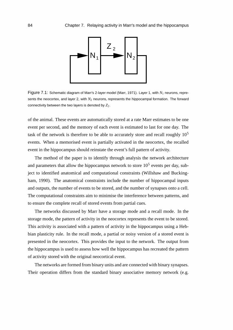
84 Chapter 7. Relaying activity in Marr’s model and the hippocampus
1N2Z
N2
Figure 7.1: Schematic diagram of Marr’s 2-layer model (Marr, 1971). Layer 1, with N1 neurons, repre-
sents the neocortex, and layer 2, with N2 neurons, represents the hippocampal formation. The forward
connectivity between the two layers is denoted by Z2.
of the animal. These events are automatically stored at a rate Marr estimates to be one
event per second, and the memory of each event is estimated to last for one day. The
task of the network is therefore to be able to accurately store and recall roughly 105
events. When a memorised event is partially activated in the neocortex, the recalled
event in the hippocampus should reinstate the event’s full pattern of activity.
The method of the paper is to identify through analysis the network architecture
and parameters that allow the hippocampus network to store 105 events per day, sub-
ject to identified anatomical and computational constraints (Willshaw and Bucking-
ham, 1990). The anatomical constraints include the number of hippocampal inputs
and outputs, the number of events to be stored, and the number of synapses onto a cell.
The computational constraints aim to minimise the interference between patterns, and
to ensure the complete recall of stored events from partial cues.
The networks discussed by Marr have a storage mode and a recall mode. In the
storage mode, the pattern of activity in the neocortex represents the event to be stored.
This activity is associated with a pattern of activity in the hippocampus using a Heb-
bian plasticity rule. In the recall mode, a partial or noisy version of a stored event is
presented in the neocortex. This provides the input to the network. The output from
the hippocampus is used to assess how well the hippocampus has recreated the pattern
of activity stored with the original neocortical event.
The networks are formed from binary units and are connected with binary synapses.
Their operation differs from the standard binary associative memory network (e.g.
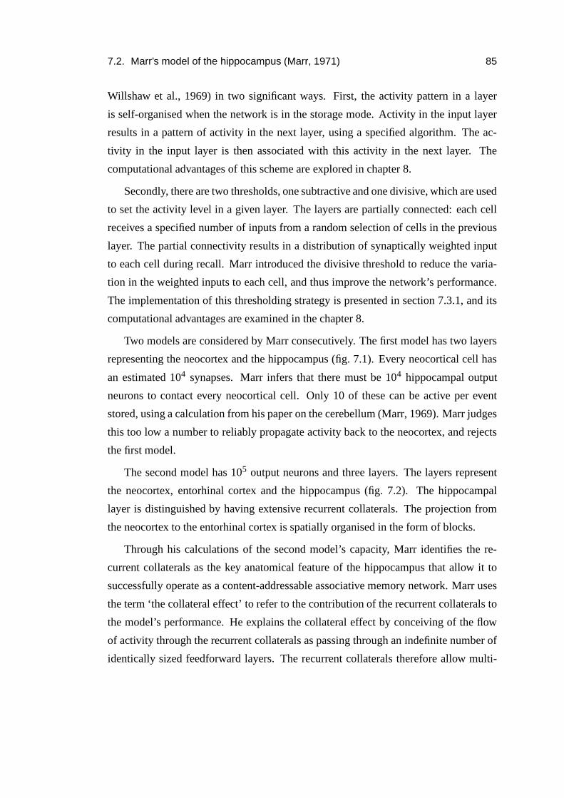
7.2. Marr’s model of the hippocampus (Marr, 1971) 85
Willshaw et al., 1969) in two significant ways. First, the activity pattern in a layer
is self-organised when the network is in the storage mode. Activity in the input layer
results in a pattern of activity in the next layer, using a specified algorithm. The ac-
tivity in the input layer is then associated with this activity in the next layer. The
computational advantages of this scheme are explored in chapter 8.
Secondly, there are two thresholds, one subtractive and one divisive, which are used
to set the activity level in a given layer. The layers are partially connected: each cell
receives a specified number of inputs from a random selection of cells in the previous
layer. The partial connectivity results in a distribution of synaptically weighted input
to each cell during recall. Marr introduced the divisive threshold to reduce the varia-
tion in the weighted inputs to each cell, and thus improve the network’s performance.
The implementation of this thresholding strategy is presented in section 7.3.1, and its
computational advantages are examined in the chapter 8.
Two models are considered by Marr consecutively. The first model has two layers
representing the neocortex and the hippocampus (fig. 7.1). Every neocortical cell has
an estimated 104 synapses. Marr infers that there must be 104 hippocampal output
neurons to contact every neocortical cell. Only 10 of these can be active per event
stored, using a calculation from his paper on the cerebellum (Marr, 1969). Marr judges
this too low a number to reliably propagate activity back to the neocortex, and rejects
the first model.
The second model has 105 output neurons and three layers. The layers represent
the neocortex, entorhinal cortex and the hippocampus (fig. 7.2). The hippocampal
layer is distinguished by having extensive recurrent collaterals. The projection from
the neocortex to the entorhinal cortex is spatially organised in the form of blocks.
Through his calculations of the second model’s capacity, Marr identifies the re-
current collaterals as the key anatomical feature of the hippocampus that allow it to
successfully operate as a content-addressable associative memory network. Marr uses
the term ‘the collateral effect’ to refer to the contribution of the recurrent collaterals to
the model’s performance. He explains the collateral effect by conceiving of the flow
of activity through the recurrent collaterals as passing through an indefinite number of
identically sized feedforward layers. The recurrent collaterals therefore allow multi-
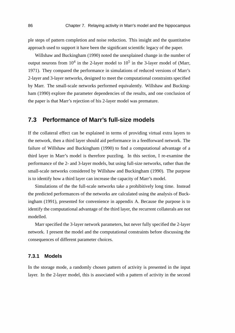
86 Chapter 7. Relaying activity in Marr’s model and the hippocampus
ple steps of pattern completion and noise reduction. This insight and the quantitative
approach used to support it have been the significant scientific legacy of the paper.
Willshaw and Buckingham (1990) noted the unexplained change in the number of
output neurons from 104 in the 2-layer model to 105 in the 3-layer model of (Marr,
1971). They compared the performance in simulations of reduced versions of Marr’s
2-layer and 3-layer networks, designed to meet the computational constraints specified
by Marr. The small-scale networks performed equivalently. Willshaw and Bucking-
ham (1990) explore the parameter dependencies of the results, and one conclusion of
the paper is that Marr’s rejection of his 2-layer model was premature.
7.3 Performance of Marr’s full-size models
If the collateral effect can be explained in terms of providing virtual extra layers to
the network, then a third layer should aid performance in a feedforward network. The
failure of Willshaw and Buckingham (1990) to find a computational advantage of a
third layer in Marr’s model is therefore puzzling. In this section, I re-examine the
performance of the 2- and 3-layer models, but using full-size networks, rather than the
small-scale networks considered by Willshaw and Buckingham (1990). The purpose
is to identify how a third layer can increase the capacity of Marr’s model.
Simulations of the the full-scale networks take a prohibitively long time. Instead
the predicted performances of the networks are calculated using the analysis of Buck-
ingham (1991), presented for convenience in appendix A. Because the purpose is to
identify the computational advantage of the third layer, the recurrent collaterals are not
modelled.
Marr specified the 3-layer network parameters, but never fully specified the 2-layer
network. I present the model and the computational constraints before discussing the
consequences of different parameter choices.
7.3.1 Models
In the storage mode, a randomly chosen pattern of activity is presented in the input
layer. In the 2-layer model, this is associated with a pattern of activity in the second
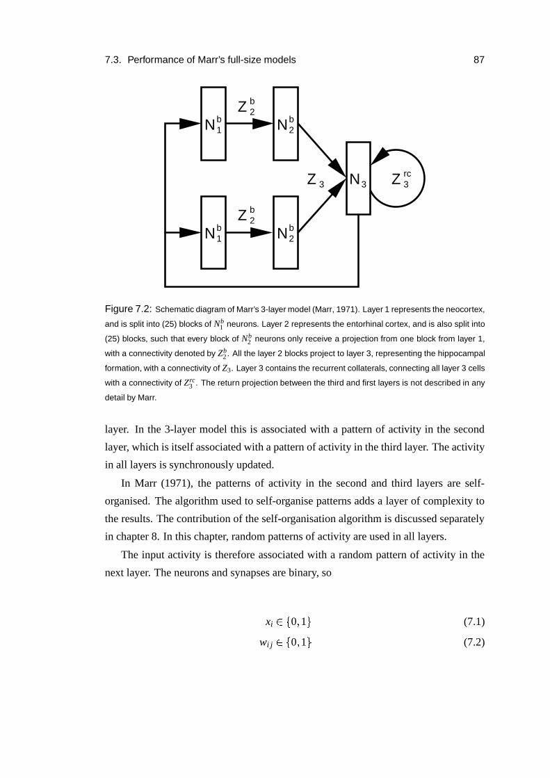
7.3. Performance of Marr’s full-size models 87
b2
b2
b1
b1N
b2Z
b2Z
3 3rc3
N
N
N
Z N Z
Figure 7.2: Schematic diagram of Marr’s 3-layer model (Marr, 1971). Layer 1 represents the neocortex,
and is split into (25) blocks of Nb1 neurons. Layer 2 represents the entorhinal cortex, and is also split into
(25) blocks, such that every block of Nb2 neurons only receive a projection from one block from layer 1,
with a connectivity denoted by Zb2 . All the layer 2 blocks project to layer 3, representing the hippocampal
formation, with a connectivity of Z3. Layer 3 contains the recurrent collaterals, connecting all layer 3 cells
with a connectivity of Zrc3 . The return projection between the third and first layers is not described in any
detail by Marr.
layer. In the 3-layer model this is associated with a pattern of activity in the second
layer, which is itself associated with a pattern of activity in the third layer. The activity
in all layers is synchronously updated.
In Marr (1971), the patterns of activity in the second and third layers are self-
organised. The algorithm used to self-organise patterns adds a layer of complexity to
the results. The contribution of the self-organisation algorithm is discussed separately
in chapter 8. In this chapter, random patterns of activity are used in all layers.
The input activity is therefore associated with a random pattern of activity in the
next layer. The neurons and synapses are binary, so
xi ��0 � 1 � (7.1)
wi j ��0 � 1 � (7.2)
88 Chapter 7. Relaying activity in Marr’s model and the hippocampus
where xi is the state of neuron i, and wi j is the synapse to neuron i from neuron j in
the previous layer.
The learning rule is all-or-none Hebbian plasticity. During the storage of an event
∆wi j � xix j � (7.3)
for an unpotentiated synapse.
In recall mode, a recall cue is presented in layer 1. The recall cue is either a stored
input pattern, or a partial or noisy version of a stored input pattern. The activity in all
layers is again synchronously updated. The recall cue is presented for one time-step in
the input layer then removed.
The state of a neuron in each time-step is calculated by thresholding the dendritic
sum. The dendritic sum, di, of neuron i is
di � ∑j
ci jwi jx j (7.4)
where ci j denotes whether there is a connection with the input neuron j. All layers
are only partially connected.
Two threshold are used, one subtractive and one divisive. The subtractive threshold,
T , operates on the dendritic sum of all cells:
xi ��
1 if di � T
0 otherwise �
(7.5)
The divisive inhibition threshold for all cells, f , selects the output units with the
greatest proportion of modified active synapses (Marr, 1971, section 3.1.2). All the
synapses connecting active input and output cells are modified during the storage of a
pattern. Therefore, output cells where the majority of its active synapses are potenti-
ated during recall are likely to have been active during storage.
The divisive threshold operates not only on the dendritic sum but also the input
activity of each cell. The input activity of neuron i, ai, is defined as
7.3. Performance of Marr’s full-size models 89
ai � ∑j
ci jx j � (7.6)
The input activity is therefore the number of active input cells that the cell is con-
nected to, whether or not the synapses are potentiated. The divisive threshold selects
the output cells with the greatest proportion of modified active synapses:
xi ��
1 if di � f ai
0 otherwise �
(7.7)
The divisive inhibition represents the effects of feedforward somatic inhibition
from a basket cell. Every cell is hypothesised to have its own basket cell which re-
ceives the same input synapses. In this way, the dendritic sum of each cell is divided
by an amount proportional to its input activity. The subtractive threshold represents
dendritic feedforward and feedback inhibition. How the values of thresholds T and f
are chosen is not properly explained (Marr, 1971, section 3.1.3, S5; section 3.3). Marr
implements the threshold cell i, as
xi ��
1 if di � max�T � f ai �
0 otherwise �
(7.8)
The task set by Marr was to be able to recall an event from a recall cue of activity
in just one block of layer 1, when 105 events have been stored in the network.
7.3.2 Methods
In this chapter, unless otherwise stated, all the results are generated by calculating the
predicted performance of a network.
In order to predict the performance of a network, the cells are first classified into
two populations which are treated as homogeneous populations. The cells that were
active during the storage of the pattern being recalled are classed as genuine cells. The
cells that were not active during storage are classed as spurious cells. The probability
90 Chapter 7. Relaying activity in Marr’s model and the hippocampus
function of the dendritic sum of a genuine neuron, P � dg � , and the probability function
of the dendritic sum of a spurious neuron, P � ds � , are calculated using the analysis
developed by (Buckingham, 1991, appendix A).
The proportion of the probability function of the dendritic sum of each class that
exceeds the subtractive and divisive thresholds, T and f, are used to calculate the ex-
pected number of active genuine neurons, E � Ng � , and the expected number of spurious
neurons, E �Ns � , in layer i:
E �Ng � � P � dg � max � T � f ag ��� � Mi (7.9)
E � Ns � � P � ds � max�T � f as � � � � Ni � Mi � (7.10)
(7.11)
where Mi is the number of active neurons in a pattern in layer i, and Ni is the total
number of neurons in layer i.
In order to determine the values of T and f during recall, the values of T and f are
chosen which minimise the hamming distance between the output and the stored pat-
tern. This method of determining T and f is referred to as the ‘omniscient’ thresholding
mechanism, after Buckingham (1991).
The omniscient thresholding mechanism sets all the output units to be inactive
when very noisy recall cues are used. To prevent inactive states in response to recall
from very noisy cues, Mµi , the number of active cells in layer i during the recall of
pattern µ, is constrained such that
2 � Mi � Mµi � Mi � 2 � (7.12)
where Mi is the number of active cells in layer i during the storage of a pattern.
The output error therefore tends to a maximum of Mi false negatives and Mi � 2 false
positives, a hamming distance of 3Mi � 2.
The performance is calculated using the activity of the output layer, and not by the
activity in layer 1. In Marr (1971), activity is allowed to cycle indefinitely through the
recurrent collaterals before being assessed. The recurrent collaterals are not modelled
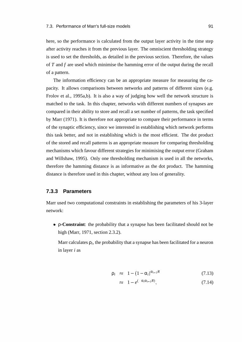
7.3. Performance of Marr’s full-size models 91
here, so the performance is calculated from the output layer activity in the time step
after activity reaches it from the previous layer. The omniscient thresholding strategy
is used to set the thresholds, as detailed in the previous section. Therefore, the values
of T and f are used which minimise the hamming error of the output during the recall
of a pattern.
The information efficiency can be an appropriate measure for measuring the ca-
pacity. It allows comparisons between networks and patterns of different sizes (e.g.
Frolov et al., 1995a,b). It is also a way of judging how well the network structure is
matched to the task. In this chapter, networks with different numbers of synapses are
compared in their ability to store and recall a set number of patterns, the task specified
by Marr (1971). It is therefore not appropriate to compare their performance in terms
of the synaptic efficiency, since we interested in establishing which network performs
this task better, and not in establishing which is the most efficient. The dot product
of the stored and recall patterns is an appropriate measure for comparing thresholding
mechanisms which favour different strategies for minimising the output error (Graham
and Willshaw, 1995). Only one thresholding mechanism is used in all the networks,
therefore the hamming distance is as informative as the dot product. The hamming
distance is therefore used in this chapter, without any loss of generality.
7.3.3 Parameters
Marr used two computational constraints in establishing the parameters of his 3-layer
network:
� ρ-Constraint: the probability that a synapse has been facilitated should not be
high (Marr, 1971, section 2.3.2).
Marr calculates ρi, the probability that a synapse has been facilitated for a neuron
in layer i as
ρi � 1 � � 1 � αi � αi � 1R (7.13)
� 1 � e���
αiαi � 1R � � (7.14)
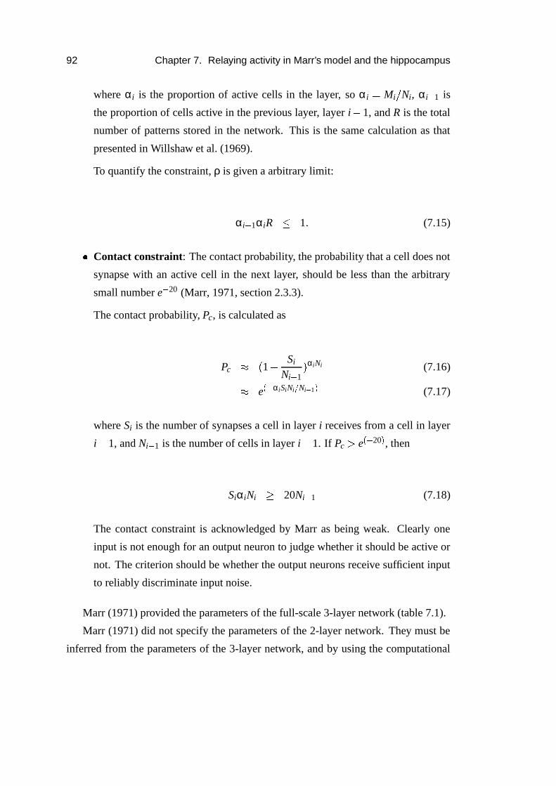
92 Chapter 7. Relaying activity in Marr’s model and the hippocampus
where αi is the proportion of active cells in the layer, so αi � Mi � Ni, αi�
1 is
the proportion of cells active in the previous layer, layer i � 1, and R is the total
number of patterns stored in the network. This is the same calculation as that
presented in Willshaw et al. (1969).
To quantify the constraint, ρ is given a arbitrary limit:
αi�
1αiR � 1 � (7.15)
� Contact constraint: The contact probability, the probability that a cell does not
synapse with an active cell in the next layer, should be less than the arbitrary
small number e�
20 (Marr, 1971, section 2.3.3).
The contact probability, Pc, is calculated as
Pc � � 1 �
Si
Ni�
1� αiNi (7.16)
� e���
αiSiNi � Ni � 1 � (7.17)
where Si is the number of synapses a cell in layer i receives from a cell in layer
i � 1, and Ni�
1 is the number of cells in layer i � 1. If Pc � e� �
20 � , then
SiαiNi � 20Ni�
1 (7.18)
The contact constraint is acknowledged by Marr as being weak. Clearly one
input is not enough for an output neuron to judge whether it should be active or
not. The criterion should be whether the output neurons receive sufficient input
to reliably discriminate input noise.
Marr (1971) provided the parameters of the full-scale 3-layer network (table 7.1).
Marr (1971) did not specify the parameters of the 2-layer network. They must be
inferred from the parameters of the 3-layer network, and by using the computational
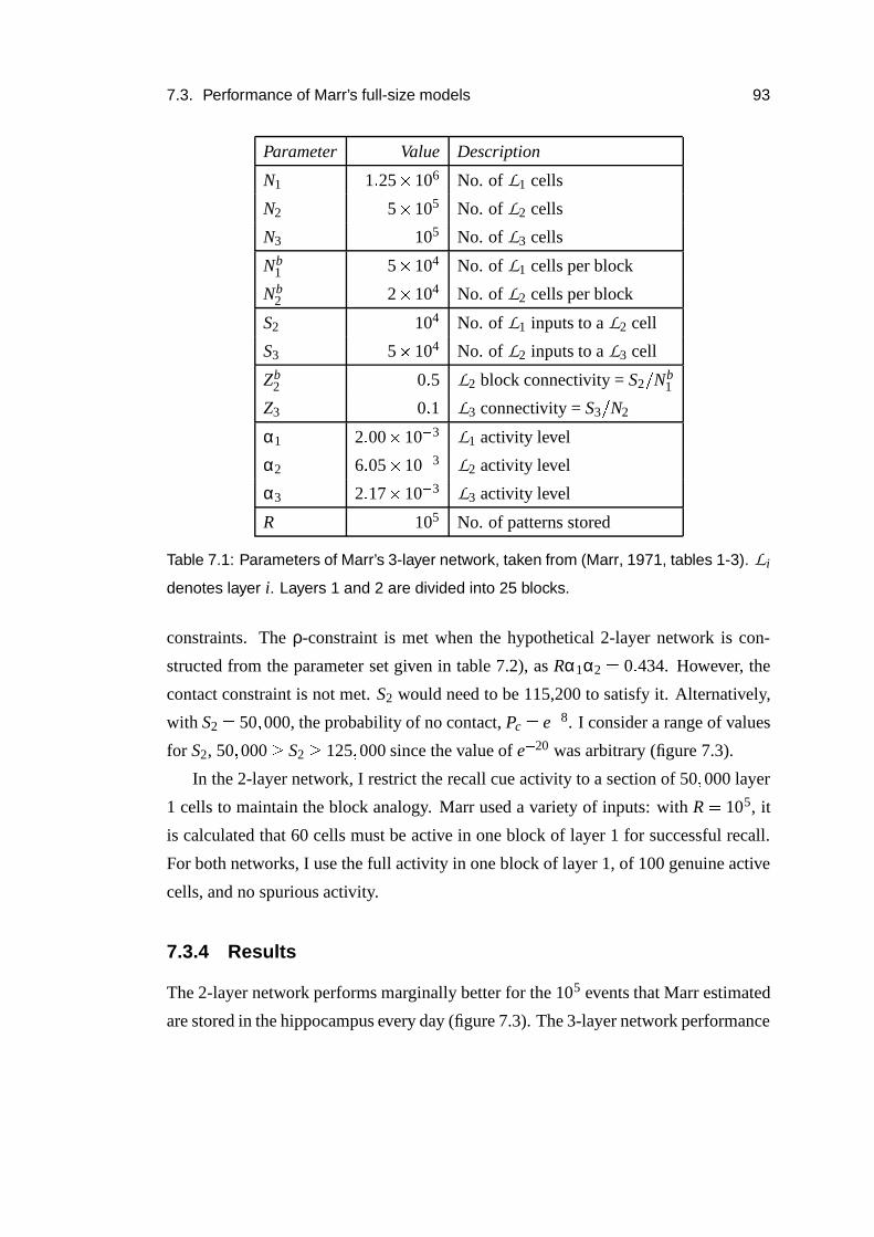
7.3. Performance of Marr’s full-size models 93
Parameter Value Description
N1 1 � 25 � 106 No. of L1 cells
N2 5 � 105 No. of L2 cells
N3 105 No. of L3 cells
Nb1 5 � 104 No. of L1 cells per block
Nb2 2 � 104 No. of L2 cells per block
S2 104 No. of L1 inputs to a L2 cell
S3 5 � 104 No. of L2 inputs to a L3 cell
Zb2 0 � 5 L2 block connectivity = S2 � Nb
1
Z3 0 � 1 L3 connectivity = S3 � N2
α1 2 � 00 � 10�
3 L1 activity level
α2 6 � 05 � 10�
3 L2 activity level
α3 2 � 17 � 10�
3 L3 activity level
R 105 No. of patterns stored
Table 7.1: Parameters of Marr’s 3-layer network, taken from (Marr, 1971, tables 1-3). Li
denotes layer i. Layers 1 and 2 are divided into 25 blocks.
constraints. The ρ-constraint is met when the hypothetical 2-layer network is con-
structed from the parameter set given in table 7.2), as Rα1α2 � 0 � 434. However, the
contact constraint is not met. S2 would need to be 115,200 to satisfy it. Alternatively,
with S2 � 50 � 000, the probability of no contact, Pc � e�
8. I consider a range of values
for S2, 50 � 000 � S2 � 125 � 000 since the value of e�
20 was arbitrary (figure 7.3).
In the 2-layer network, I restrict the recall cue activity to a section of 50 � 000 layer
1 cells to maintain the block analogy. Marr used a variety of inputs: with R � 105, it
is calculated that 60 cells must be active in one block of layer 1 for successful recall.
For both networks, I use the full activity in one block of layer 1, of 100 genuine active
cells, and no spurious activity.
7.3.4 Results
The 2-layer network performs marginally better for the 105 events that Marr estimated
are stored in the hippocampus every day (figure 7.3). The 3-layer network performance
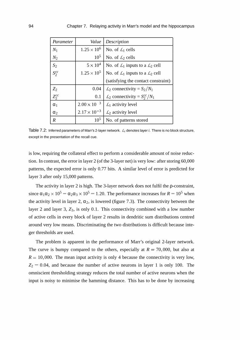
94 Chapter 7. Relaying activity in Marr’s model and the hippocampus
Parameter Value Description
N1 1 � 25 � 106 No. of L1 cells
N2 105 No. of L2 cells
S2 5 � 104 No. of L1 inputs to a L2 cell
Scc2 1 � 25 � 105 No. of L1 inputs to a L2 cell
(satisfying the contact constraint)
Z2 0 � 04 L2 connectivity = S2 � N1
Zcc2 0 � 1 L2 connectivity = Scc
2 � N1
α1 2 � 00 � 10�
3 L1 activity level
α2 2 � 17 � 10�
3 L2 activity level
R 105 No. of patterns stored
Table 7.2: Inferred parameters of Marr’s 2-layer network. Li denotes layer i. There is no block structure,
except in the presentation of the recall cue.
is low, requiring the collateral effect to perform a considerable amount of noise reduc-
tion. In contrast, the error in layer 2 (of the 3-layer net) is very low: after storing 60,000
patterns, the expected error is only 0.77 bits. A similar level of error is predicted for
layer 3 after only 15,000 patterns.
The activity in layer 2 is high. The 3-layer network does not fulfil the ρ-constraint,
since α1α2� 105 � α2α3
� 105 � 1 � 20. The performance increases for R � 105 when
the activity level in layer 2, α2, is lowered (figure 7.3). The connectivity between the
layer 2 and layer 3, Z3, is only 0 � 1. This connectivity combined with a low number
of active cells in every block of layer 2 results in dendritic sum distributions centred
around very low means. Discriminating the two distributions is difficult because inte-
ger thresholds are used.
The problem is apparent in the performance of Marr’s original 2-layer network.
The curve is bumpy compared to the others, especially at R � 70 � 000, but also at
R � 10 � 000. The mean input activity is only 4 because the connectivity is very low,
Z2 � 0 � 04, and because the number of active neurons in layer 1 is only 100. The
omniscient thresholding strategy reduces the total number of active neurons when the
input is noisy to minimise the hamming distance. This has to be done by increasing
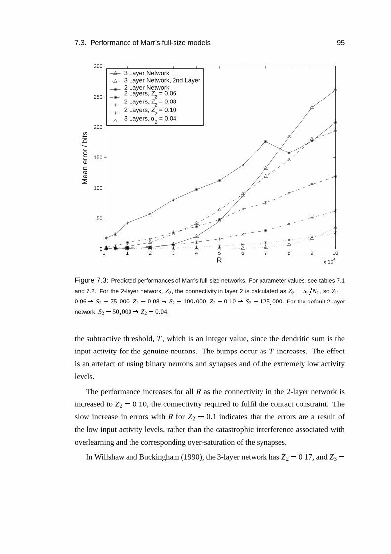
7.3. Performance of Marr’s full-size models 95
0 1 2 3 4 5 6 7 8 9 10
x 104
0
50
100
150
200
250
300
R
Mea
n er
ror
/ bits
3 Layer Network3 Layer Network, 2nd Layer2 Layer Network2 Layers, Z
2 = 0.06
2 Layers, Z2 = 0.08
2 Layers, Z2 = 0.10
3 Layers, α2 = 0.04
Figure 7.3: Predicted performances of Marr’s full-size networks. For parameter values, see tables 7.1
and 7.2. For the 2-layer network, Z2, the connectivity in layer 2 is calculated as Z2 � S2�N1, so Z2 �
0 � 06 � S2 � 75 � 000, Z2 � 0 � 08 � S2 � 100 � 000, Z2 � 0 � 10 � S2 � 125 � 000. For the default 2-layer
network, S2 � 50 � 000 � Z2 � 0 � 04.
the subtractive threshold, T , which is an integer value, since the dendritic sum is the
input activity for the genuine neurons. The bumps occur as T increases. The effect
is an artefact of using binary neurons and synapses and of the extremely low activity
levels.
The performance increases for all R as the connectivity in the 2-layer network is
increased to Z2 � 0 � 10, the connectivity required to fulfil the contact constraint. The
slow increase in errors with R for Z2 � 0 � 1 indicates that the errors are a result of
the low input activity levels, rather than the catastrophic interference associated with
overlearning and the corresponding over-saturation of the synapses.
In Willshaw and Buckingham (1990), the 3-layer network has Z2 � 0 � 17, and Z3 �
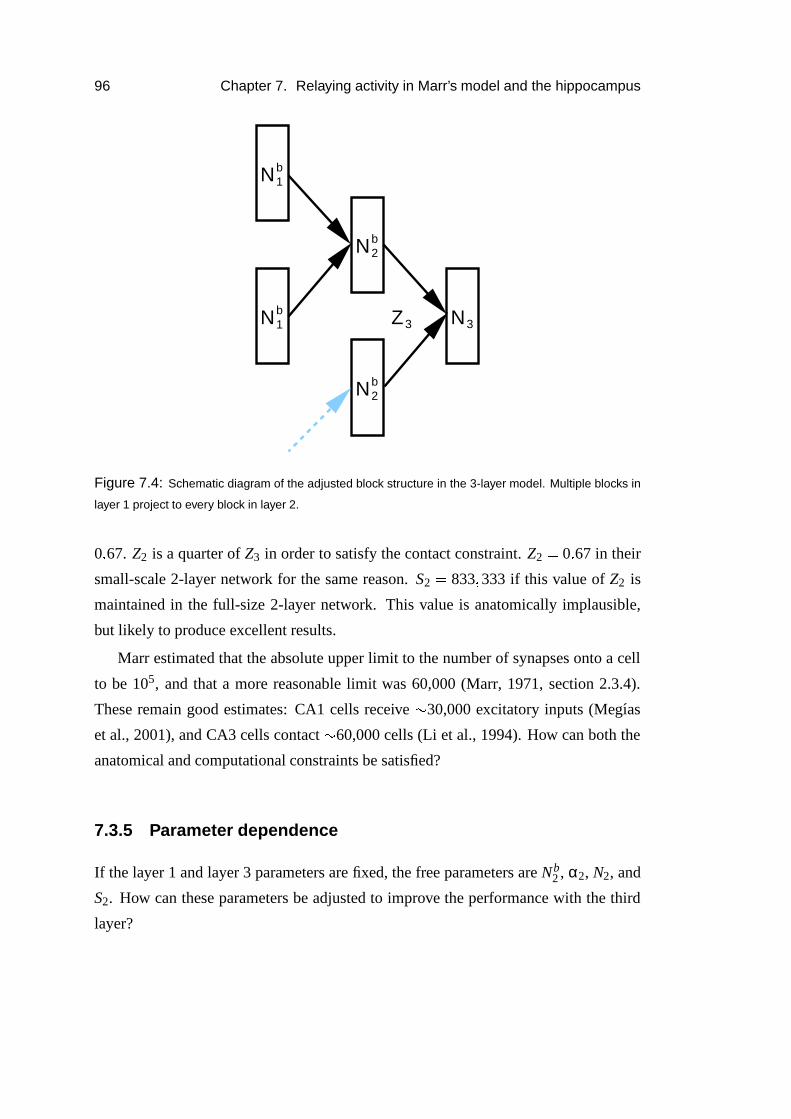
96 Chapter 7. Relaying activity in Marr’s model and the hippocampus
b2
b1
b1
N
NZ
N
3
N
N
b2
3
Figure 7.4: Schematic diagram of the adjusted block structure in the 3-layer model. Multiple blocks in
layer 1 project to every block in layer 2.
0 � 67. Z2 is a quarter of Z3 in order to satisfy the contact constraint. Z2 � 0 � 67 in their
small-scale 2-layer network for the same reason. S2 � 833 � 333 if this value of Z2 is
maintained in the full-size 2-layer network. This value is anatomically implausible,
but likely to produce excellent results.
Marr estimated that the absolute upper limit to the number of synapses onto a cell
to be 105, and that a more reasonable limit was 60,000 (Marr, 1971, section 2.3.4).
These remain good estimates: CA1 cells receive � 30,000 excitatory inputs (Megıas
et al., 2001), and CA3 cells contact � 60,000 cells (Li et al., 1994). How can both the
anatomical and computational constraints be satisfied?
7.3.5 Parameter dependence
If the layer 1 and layer 3 parameters are fixed, the free parameters are Nb2 , α2, N2, and
S2. How can these parameters be adjusted to improve the performance with the third
layer?
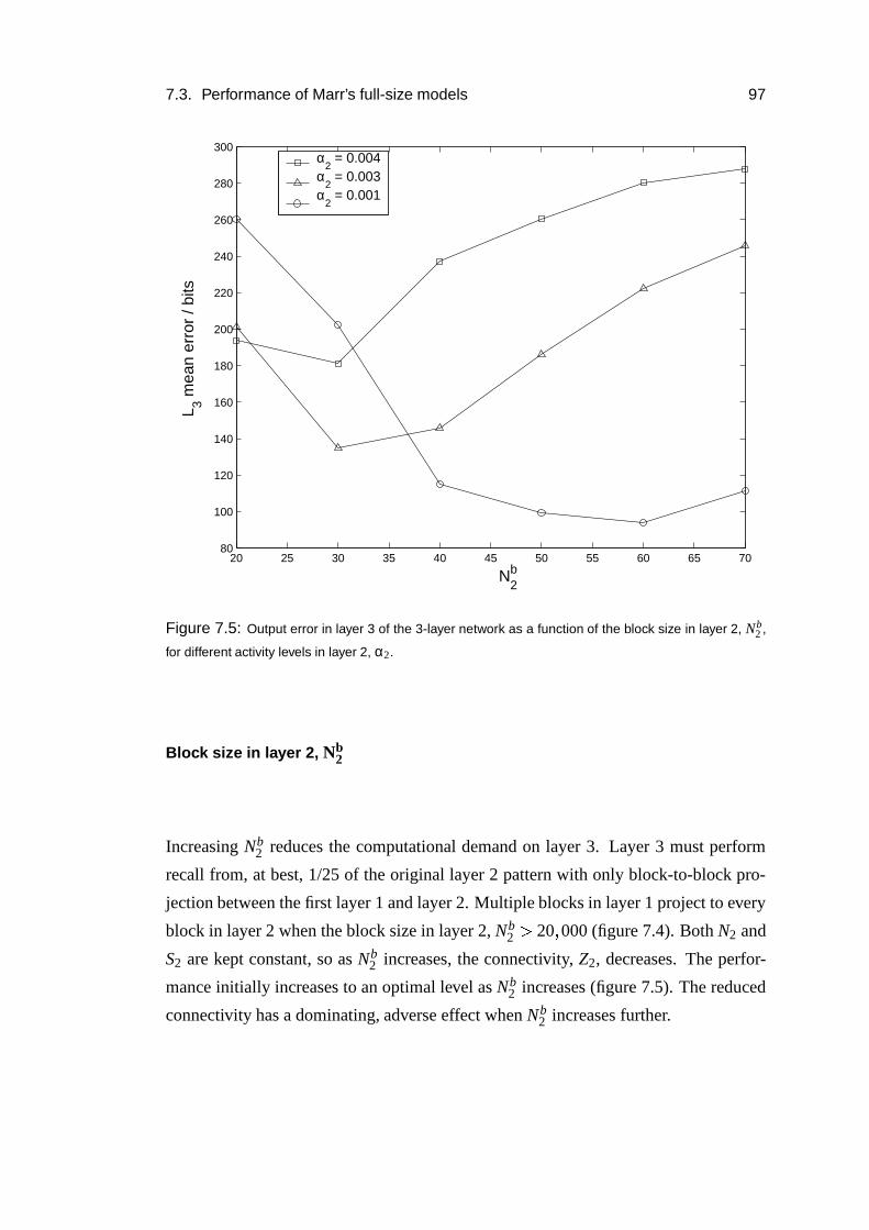
7.3. Performance of Marr’s full-size models 97
20 25 30 35 40 45 50 55 60 65 7080
100
120
140
160
180
200
220
240
260
280
300
N2b
L 3 mea
n er
ror
/ bits
α2 = 0.004
α2 = 0.003
α2 = 0.001
Figure 7.5: Output error in layer 3 of the 3-layer network as a function of the block size in layer 2, Nb2 ,
for different activity levels in layer 2, α2.
Block size in layer 2, Nb2
Increasing Nb2 reduces the computational demand on layer 3. Layer 3 must perform
recall from, at best, 1/25 of the original layer 2 pattern with only block-to-block pro-
jection between the first layer 1 and layer 2. Multiple blocks in layer 1 project to every
block in layer 2 when the block size in layer 2, Nb2 � 20 � 000 (figure 7.4). Both N2 and
S2 are kept constant, so as Nb2 increases, the connectivity, Z2, decreases. The perfor-
mance initially increases to an optimal level as Nb2 increases (figure 7.5). The reduced
connectivity has a dominating, adverse effect when Nb2 increases further.
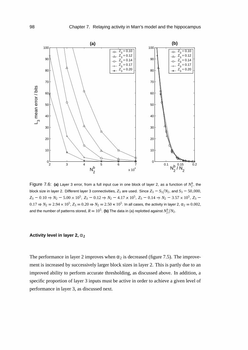
98 Chapter 7. Relaying activity in Marr’s model and the hippocampus
0.1 0.15 0.20
10
20
30
40
50
60
70
80
90
100(b)
N2b / N
2
2 3 4 5 6 7
x 104
0
10
20
30
40
50
60
70
80
90
100
N2b
(a)
L 3 mea
n er
ror
/ bits
Z3 = 0.10
Z3 = 0.12
Z3 = 0.14
Z3 = 0.17
Z3 = 0.20
Z3 = 0.10
Z3 = 0.12
Z3 = 0.14
Z3 = 0.17
Z3 = 0.20
Figure 7.6: (a) Layer 3 error, from a full input cue in one block of layer 2, as a function of Nb2 , the
block size in layer 2. Different layer 3 connectivities, Z3 are used. Since Z3 � S3�N2, and S3 � 50 � 000,
Z3 � 0 � 10 � N2 � 5 � 00 � 105, Z3 � 0 � 12 � N2 � 4 � 17 � 105, Z3 � 0 � 14 � N2 � 3 � 57 � 105, Z3 �
0 � 17 � N2 � 2 � 94 � 105, Z3 � 0 � 20 � N2 � 2 � 50 � 105. In all cases, the activity in layer 2, α2 � 0 � 002,
and the number of patterns stored, R � 105. (b) The data in (a) replotted against Nb2
�N2.
Activity level in layer 2, α2
The performance in layer 2 improves when α2 is decreased (figure 7.5). The improve-
ment is increased by successively larger block sizes in layer 2. This is partly due to an
improved ability to perform accurate thresholding, as discussed above. In addition, a
specific proportion of layer 3 inputs must be active in order to achieve a given level of
performance in layer 3, as discussed next.
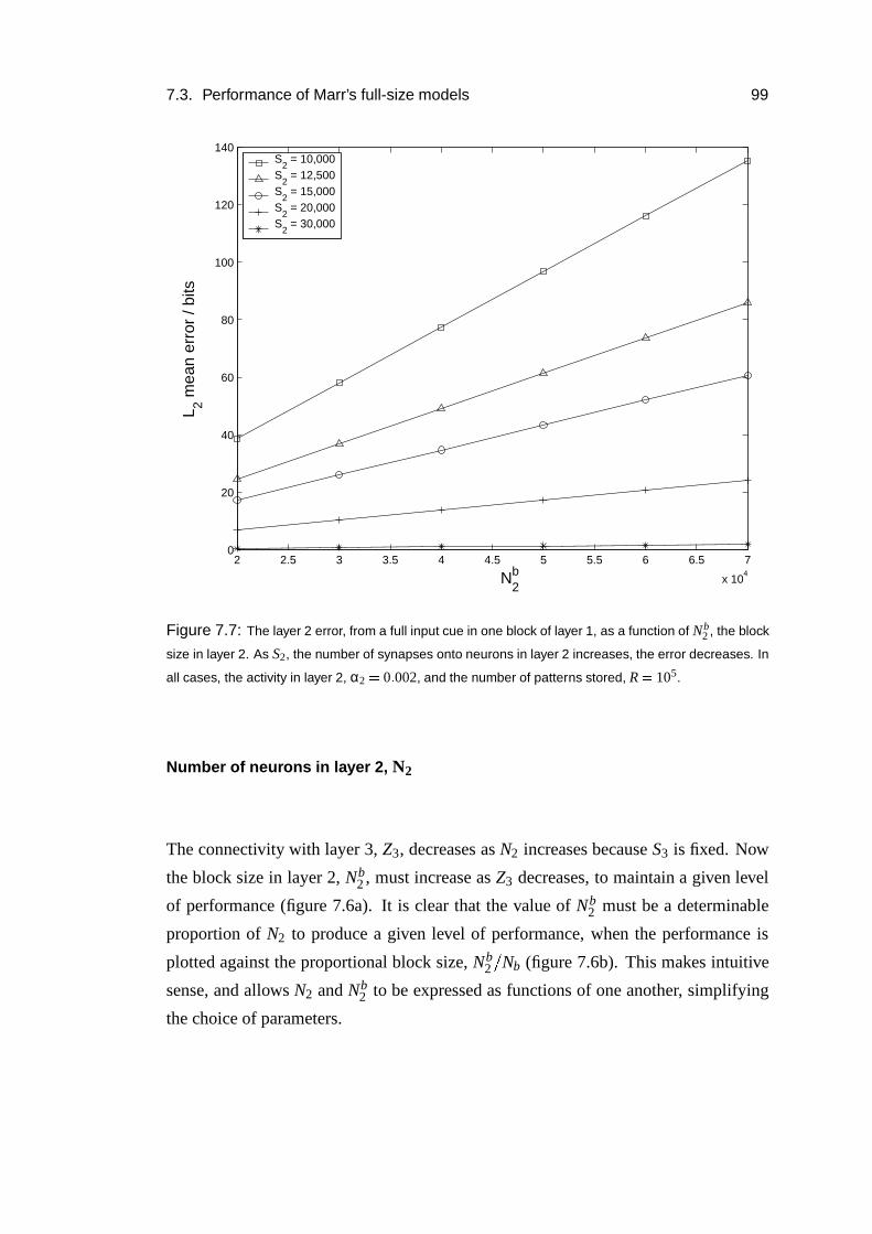
7.3. Performance of Marr’s full-size models 99
2 2.5 3 3.5 4 4.5 5 5.5 6 6.5 7
x 104
0
20
40
60
80
100
120
140
N2b
L 2 mea
n er
ror
/ bits
S2 = 10,000
S2 = 12,500
S2 = 15,000
S2 = 20,000
S2 = 30,000
Figure 7.7: The layer 2 error, from a full input cue in one block of layer 1, as a function of Nb2 , the block
size in layer 2. As S2, the number of synapses onto neurons in layer 2 increases, the error decreases. In
all cases, the activity in layer 2, α2 � 0 � 002, and the number of patterns stored, R � 105.
Number of neurons in layer 2, N2
The connectivity with layer 3, Z3, decreases as N2 increases because S3 is fixed. Now
the block size in layer 2, Nb2 , must increase as Z3 decreases, to maintain a given level
of performance (figure 7.6a). It is clear that the value of Nb2 must be a determinable
proportion of N2 to produce a given level of performance, when the performance is
plotted against the proportional block size, Nb2 � Nb (figure 7.6b). This makes intuitive
sense, and allows N2 and Nb2 to be expressed as functions of one another, simplifying
the choice of parameters.
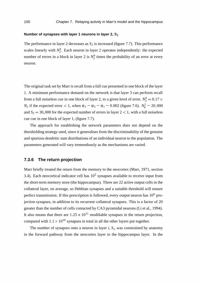
100 Chapter 7. Relaying activity in Marr’s model and the hippocampus
Number of synapses with layer 1 neurons in layer 2, S2
The performance in layer 2 decreases as S2 is increased (figure 7.7). This performance
scales linearly with Nb2 . Each neuron in layer 2 operates independently: the expected
number of errors in a block in layer 2 is Nb2 times the probability of an error at every
neuron.
The original task set by Marr is recall from a full cue presented in one block of the layer
1. A minimum performance demand on the network is that layer 3 can perform recall
from a full noiseless cue in one block of layer 2, to a given level of error. Nb2 � 0 � 17 �
N2 if the expected error � 1, when α2 � α3 � α1 � 0 � 002 (figure 7.6). N2b � 20 � 000
and S2 � 30 � 000 for the expected number of errors in layer 2 � 1, with a full noiseless
cue cue in one block of layer 1, (figure 7.7).
The approach for establishing the network parameters does not depend on the
thresholding strategy used, since it generalises from the discriminability of the genuine
and spurious dendritic sum distributions of an individual neuron to the population. The
parameters generated will vary tremendously as the mechanisms are varied.
7.3.6 The return projection
Marr briefly treated the return from the memory to the neocortex (Marr, 1971, section
3.4). Each neocortical indicator cell has 105 synapses available to receive input from
the short-term memory store (the hippocampus). There are 22 active output cells in the
collateral layer, on average, so Hebbian synapses and a suitable threshold will ensure
perfect transmission. If this prescription is followed, every output neuron has 106 pro-
jection synapses, in addition to its recurrent collateral synapses. This is a factor of 20
greater than the number of cells contacted by CA3 pyramidal neurons (Li et al., 1994).
It also means that there are 1 � 25 � 1011 modifiable synapses in the return projection,
compared with 1 � 1 � 1010 synapses in total in all the other layers put together.
The number of synapses onto a neuron in layer i, Si, was constrained by anatomy
in the forward pathway from the neocortex layer to the hippocampus layer. In the
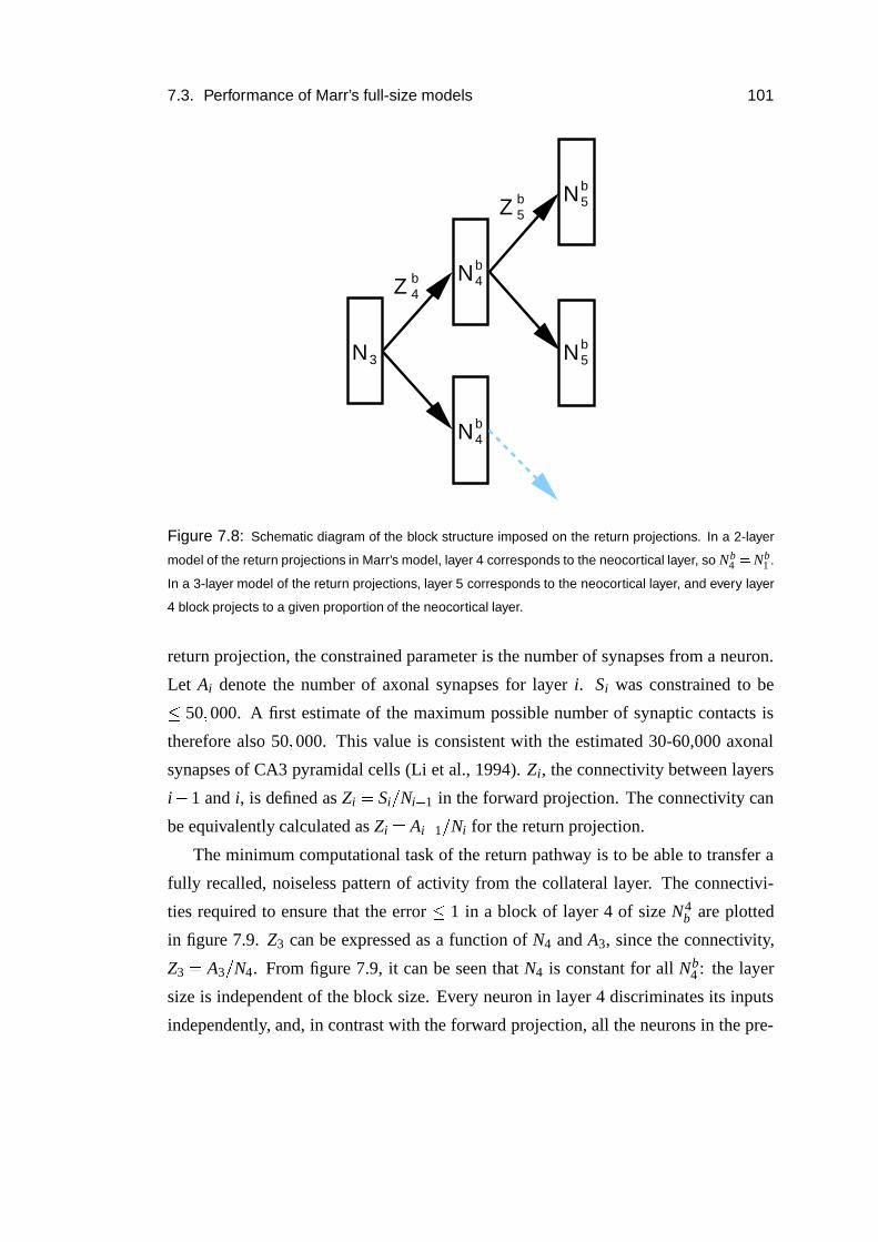
7.3. Performance of Marr’s full-size models 101
b4
b5
b5
b4Nb
4Z
b5
N
N
N
N3
Z
Figure 7.8: Schematic diagram of the block structure imposed on the return projections. In a 2-layer
model of the return projections in Marr’s model, layer 4 corresponds to the neocortical layer, so Nb4 � Nb
1 .
In a 3-layer model of the return projections, layer 5 corresponds to the neocortical layer, and every layer
4 block projects to a given proportion of the neocortical layer.
return projection, the constrained parameter is the number of synapses from a neuron.
Let Ai denote the number of axonal synapses for layer i. Si was constrained to be
� 50 � 000. A first estimate of the maximum possible number of synaptic contacts is
therefore also 50 � 000. This value is consistent with the estimated 30-60,000 axonal
synapses of CA3 pyramidal cells (Li et al., 1994). Zi, the connectivity between layers
i � 1 and i, is defined as Zi � Si � Ni�
1 in the forward projection. The connectivity can
be equivalently calculated as Zi � Ai�
1 � Ni for the return projection.
The minimum computational task of the return pathway is to be able to transfer a
fully recalled, noiseless pattern of activity from the collateral layer. The connectivi-
ties required to ensure that the error � 1 in a block of layer 4 of size N4b are plotted
in figure 7.9. Z3 can be expressed as a function of N4 and A3, since the connectivity,
Z3 � A3 � N4. From figure 7.9, it can be seen that N4 is constant for all Nb4 : the layer
size is independent of the block size. Every neuron in layer 4 discriminates its inputs
independently, and, in contrast with the forward projection, all the neurons in the pre-
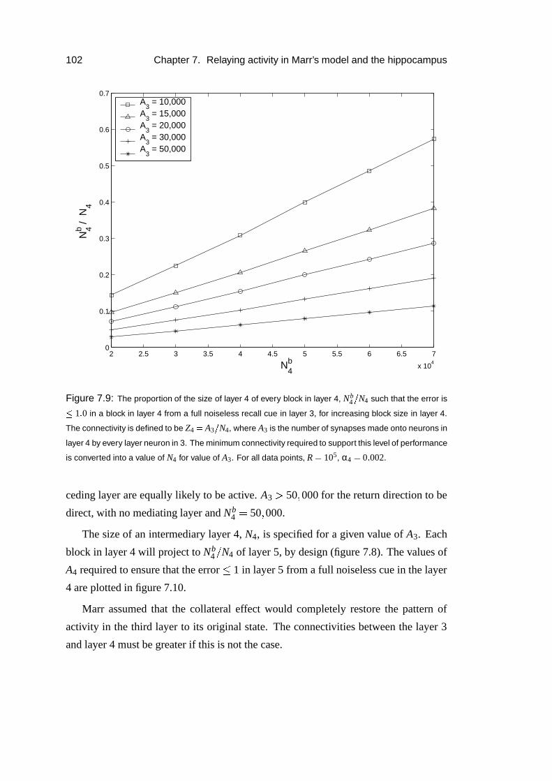
102 Chapter 7. Relaying activity in Marr’s model and the hippocampus
2 2.5 3 3.5 4 4.5 5 5.5 6 6.5 7
x 104
0
0.1
0.2
0.3
0.4
0.5
0.6
0.7N
4b / N
4
N4b
A3 = 10,000
A3 = 15,000
A3 = 20,000
A3 = 30,000
A3 = 50,000
Figure 7.9: The proportion of the size of layer 4 of every block in layer 4, Nb4
�N4 such that the error is
�1 � 0 in a block in layer 4 from a full noiseless recall cue in layer 3, for increasing block size in layer 4.
The connectivity is defined to be Z4 � A3�N4, where A3 is the number of synapses made onto neurons in
layer 4 by every layer neuron in 3. The minimum connectivity required to support this level of performance
is converted into a value of N4 for value of A3. For all data points, R � 105, α4 � 0 � 002.
ceding layer are equally likely to be active. A3 � 50 � 000 for the return direction to be
direct, with no mediating layer and Nb4 � 50 � 000.
The size of an intermediary layer 4, N4, is specified for a given value of A3. Each
block in layer 4 will project to Nb4 � N4 of layer 5, by design (figure 7.8). The values of
A4 required to ensure that the error � 1 in layer 5 from a full noiseless cue in the layer
4 are plotted in figure 7.10.
Marr assumed that the collateral effect would completely restore the pattern of
activity in the third layer to its original state. The connectivities between the layer 3
and layer 4 must be greater if this is not the case.
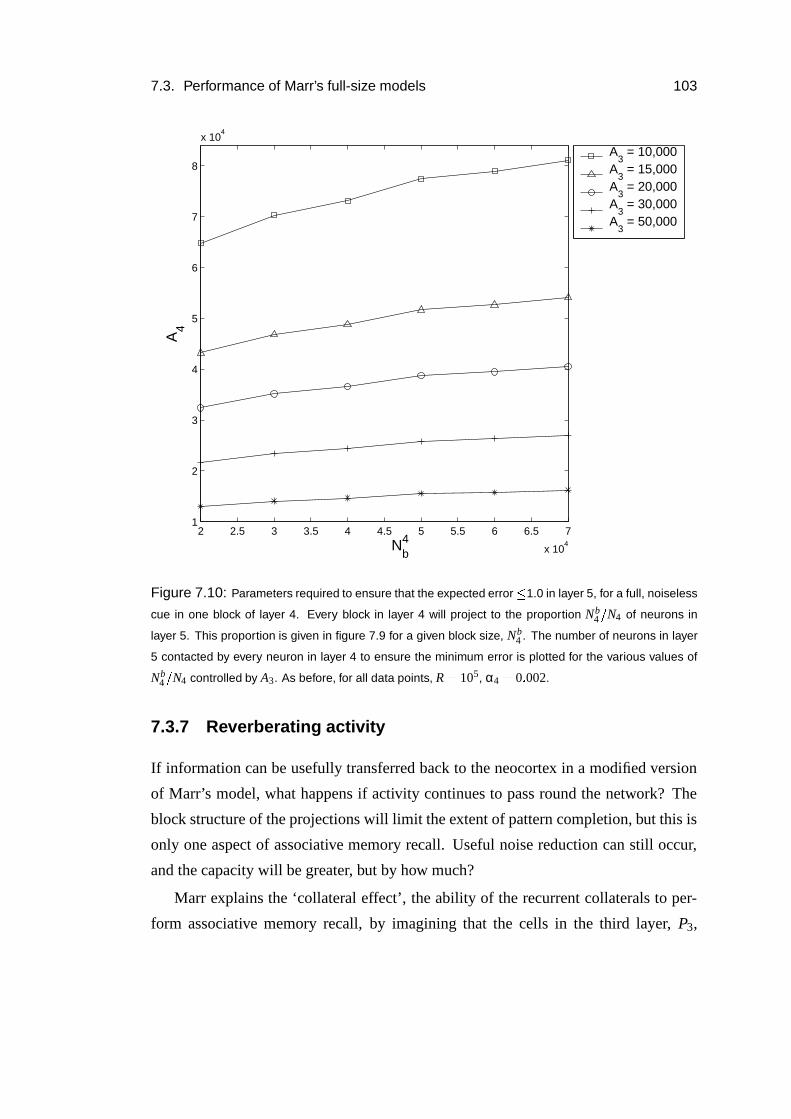
7.3. Performance of Marr’s full-size models 103
2 2.5 3 3.5 4 4.5 5 5.5 6 6.5 7
x 104
1
2
3
4
5
6
7
8
x 104
Nb4
A4
A3 = 10,000
A3 = 15,000
A3 = 20,000
A3 = 30,000
A3 = 50,000
Figure 7.10: Parameters required to ensure that the expected error�
1.0 in layer 5, for a full, noiseless
cue in one block of layer 4. Every block in layer 4 will project to the proportion Nb4
�N4 of neurons in
layer 5. This proportion is given in figure 7.9 for a given block size, Nb4 . The number of neurons in layer
5 contacted by every neuron in layer 4 to ensure the minimum error is plotted for the various values of
Nb4
�N4 controlled by A3. As before, for all data points, R � 105, α4 � 0 � 002.
7.3.7 Reverberating activity
If information can be usefully transferred back to the neocortex in a modified version
of Marr’s model, what happens if activity continues to pass round the network? The
block structure of the projections will limit the extent of pattern completion, but this is
only one aspect of associative memory recall. Useful noise reduction can still occur,
and the capacity will be greater, but by how much?
Marr explains the ‘collateral effect’, the ability of the recurrent collaterals to per-
form associative memory recall, by imagining that the cells in the third layer, P3,
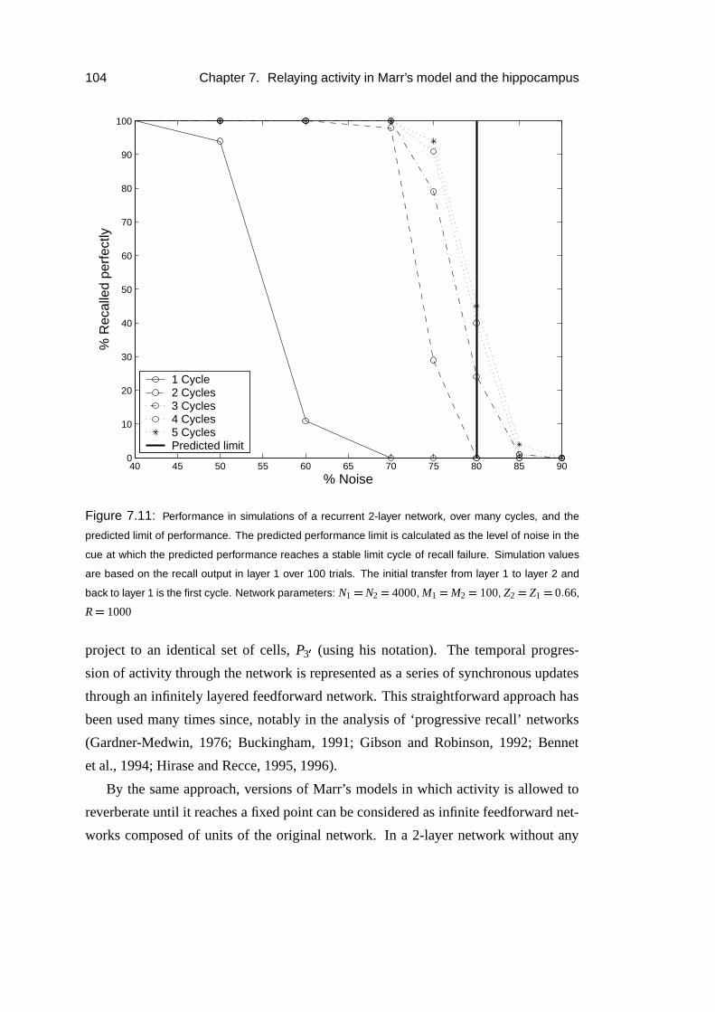
104 Chapter 7. Relaying activity in Marr’s model and the hippocampus
40 45 50 55 60 65 70 75 80 85 900
10
20
30
40
50
60
70
80
90
100
% Noise
% R
ecal
led
perf
ectly
1 Cycle2 Cycles3 Cycles4 Cycles5 CyclesPredicted limit
Figure 7.11: Performance in simulations of a recurrent 2-layer network, over many cycles, and the
predicted limit of performance. The predicted performance limit is calculated as the level of noise in the
cue at which the predicted performance reaches a stable limit cycle of recall failure. Simulation values
are based on the recall output in layer 1 over 100 trials. The initial transfer from layer 1 to layer 2 and
back to layer 1 is the first cycle. Network parameters: N1 � N2 � 4000, M1 � M2 � 100, Z2 � Z1 � 0 � 66,
R � 1000
project to an identical set of cells, P3 � (using his notation). The temporal progres-
sion of activity through the network is represented as a series of synchronous updates
through an infinitely layered feedforward network. This straightforward approach has
been used many times since, notably in the analysis of ‘progressive recall’ networks
(Gardner-Medwin, 1976; Buckingham, 1991; Gibson and Robinson, 1992; Bennet
et al., 1994; Hirase and Recce, 1995, 1996).
By the same approach, versions of Marr’s models in which activity is allowed to
reverberate until it reaches a fixed point can be considered as infinite feedforward net-
works composed of units of the original network. In a 2-layer network without any
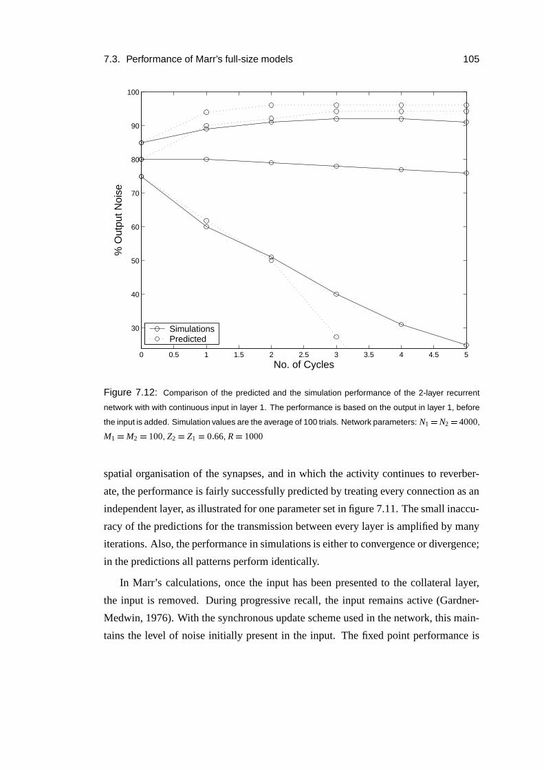
7.3. Performance of Marr’s full-size models 105
0 0.5 1 1.5 2 2.5 3 3.5 4 4.5 5
30
40
50
60
70
80
90
100
% O
utpu
t Noi
se
No. of Cycles
SimulationsPredicted
Figure 7.12: Comparison of the predicted and the simulation performance of the 2-layer recurrent
network with with continuous input in layer 1. The performance is based on the output in layer 1, before
the input is added. Simulation values are the average of 100 trials. Network parameters: N1 � N2 � 4000,
M1 � M2 � 100, Z2 � Z1 � 0 � 66, R � 1000
spatial organisation of the synapses, and in which the activity continues to reverber-
ate, the performance is fairly successfully predicted by treating every connection as an
independent layer, as illustrated for one parameter set in figure 7.11. The small inaccu-
racy of the predictions for the transmission between every layer is amplified by many
iterations. Also, the performance in simulations is either to convergence or divergence;
in the predictions all patterns perform identically.
In Marr’s calculations, once the input has been presented to the collateral layer,
the input is removed. During progressive recall, the input remains active (Gardner-
Medwin, 1976). With the synchronous update scheme used in the network, this main-
tains the level of noise initially present in the input. The fixed point performance is
106 Chapter 7. Relaying activity in Marr’s model and the hippocampus
therefore dictated by the level of noise which the network can tolerate being added to
a complete and noiseless input without affecting a perfect output. In response to high
levels of input noise, the error minimisation of the threshold setting reduces the output
activity level. The mean of the genuine dendritic sum distribution will be greater than
the mean of the spurious dendritic sum distribution. The threshold acts to increase the
ratio of genuine to spurious inputs to the next layer where possible. If in the first step
this ratio increases, recall will be successful. This process is illustrated in an exemplar
network in figure 7.12. Re-presenting the initial input on a successful recall trajectory
cannot decrease the ratio of genuine to spurious activity below its original level, and
prolongs the course of the trajectory to a steady state.
7.4 Application to the hippocampus
7.4.1 CA1 as a relay
Marr’s model can be used to investigate whether or not CA1 increases the capacity
of the CA3 projection to the subiculum and entorhinal cortex. In this section, Marr’s
2-layer and 3-layer models are parameterised to represent the projection from CA3
to the cortex and the subiculum, with and without CA1. The performances of these
two networks are then compared to quantify the contribution of the CA1 layer to the
network capacity.
It should be noted that this comparison is not controlled in that the number of
neurons and synapses in each network is not constant. A controlled comparison is
impossible to achieve, because neither the anatomical constraints nor the implentation
costs of neurons are known. I assume that CA3, the subiculum and the deep layers
of the entorhinal cortex are already optimised to perform their functions. Therefore
including the number of CA1 neurons or synapses in these areas would decrease their
performance, nullifying the control.
When Marr’s model is used to model the pathways from CA3 to the entorhinal
cortex and subiculum, the synapses are simplified to binary synapses capable of sup-
porting one-shot learning. The Schaffer collaterals synapses in CA1 are known to be
highly plastic (Bliss and Collingridge, 1993), consistent with this assumption. How-
7.4. Application to the hippocampus 107
ever, it is not clear if the assumption is valid for the synapses in the pathways from
CA1. The CA1 projection to the subiculum exhibits robust LTP (O’Mara et al., 2000),
as do the deep layers of the entorhinal cortex (Yun et al., 2002). It remains to be
determined whether or not this plasticity supports one-shot learning.
The low activity levels of hippocampal neurons have been cited as evidence consis-
tent with the function of the hippocampus as an associative memory network (Barnes
et al., 1990), since sparse activity patterns significantly enhance the memory and in-
formation capacity of such networks (Meunier et al., 1991). If the activity levels in
the subiculum and entorhinal cortex are significantly greater than in the hippocampus,
then, by this argument, this would imply that the pathways from CA1 to the subicu-
lum and entorhinal cortex do not operate as associative memory networks. Recent
experimental recordings indicate that average rates of subicular and deep entorhinal
neurons during hippocampus-dependent tasks are comparable to the average rates of
hippocampal neurons (Hampson and Deadwyler, 2003; Frank et al., 2001). This is in
contrast to earlier studies, which reported average rates an order of magnitude greater
(Sharp, 1999; Quirk et al., 1992).
The pattern completion properties of the recurrent collaterals can be expected to
settle on a pattern of activity. The pathways from CA3 are therefore unlikely to be
required to perform pattern completion. Useful noise reduction can be performed in
the return pathways for noisy, nearly recalled patterns in CA3. The performance of the
network is therefore measured using recall from full-size, noisy cues.
Model parameters
Estimates of the numbers of neurons are given in table 7.3. There are considerable
variations between rat strains (Amaral et al., 1990). Numbers for the Sprague-Dawley
strain have been used here.
The number of ipsilateral cells contacted by every CA3 cell has been estimated
in detail (see table 7.3). The numbers of subicular and entorhinal cells contacted by
every CA1 pyramidal cell are not known. It is assumed that CA1 pyramidal cells can
contact the same number of cells as CA3 pyramidal cells, and that they contact the
subicular and entorhinal neurons equally. I assume that every CA3 pyramidal cell has
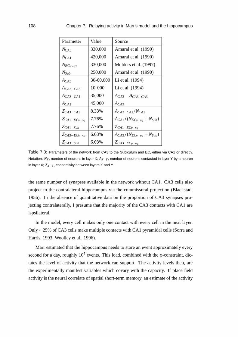
108 Chapter 7. Relaying activity in Marr’s model and the hippocampus
Parameter Value Source
NCA3 330,000 Amaral et al. (1990)
NCA1 420,000 Amaral et al. (1990)
NECV � VI 330,000 Mulders et al. (1997)
NSub 250,000 Amaral et al. (1990)
ACA3 30-60,000 Li et al. (1994)
ACA3�
CA3 10 � 000 Li et al. (1994)
ACA3�
CA1 35,000 ACA3 � ACA3�
CA3
ACA1 45,000 ACA3
ZCA3�
CA1 8.33% ACA3�
CA1 � NCA1
ZCA1�
ECV � VI 7.76% ACA1 � � NECV � V I
�NSub �
ZCA1�
Sub 7.76% ZCA1�
ECV � V I
ZCA3�
ECV � VI 6.03% ACA3 � � NECV � V I
�NSub �
ZCA3�
Sub 6.03% ZCA3�
ECV � V I
Table 7.3: Parameters of the network from CA3 to the Subiculum and EC, either via CA1 or directly.
Notation: NX , number of neurons in layer X; AX � Y , number of neurons contacted in layer Y by a neuron
in layer X; ZX � Y , connectivity between layers X and Y.
the same number of synapses available in the network without CA1. CA3 cells also
project to the contralateral hippocampus via the commissural projection (Blackstad,
1956). In the absence of quantitative data on the proportion of CA3 synapses pro-
jecting contralaterally, I presume that the majority of the CA3 contacts with CA1 are
ispsilateral.
In the model, every cell makes only one contact with every cell in the next layer.
Only � 25% of CA3 cells make multiple contacts with CA1 pyramidal cells (Sorra and
Harris, 1993; Woolley et al., 1996).
Marr estimated that the hippocampus needs to store an event approximately every
second for a day, roughly 105 events. This load, combined with the ρ-constraint, dic-
tates the level of activity that the network can support. The activity levels then, are
the experimentally manifest variables which covary with the capacity. If place field
activity is the neural correlate of spatial short-term memory, an estimate of the activity
7.4. Application to the hippocampus 109
levels can be derived.
Less than a third of hippocampal place fields will be active in a given environment,
roughly � 12% (Thompson and Best, 1989). Those active have a mean rate of � 1.0
Hz (e.g. Frank et al., 2000). If one time step in Marr’s model is equivalent to one
θ-cycle of approximately 100 ms, this is 0.1 spikes per time step. The probability of
successful synaptic transmission is � 0.5 (Rosenmund et al., 1993). The probability of
transmission is perhaps best included as a separate variable (e.g. Gibson et al., 1991;
Graham and Willshaw, 1999), but here I will consider the effect of its mean value on
the firing rate. The resulting order of magnitude estimate for the activity is between
0.015 and 0.001.
The activity levels of the subiculum and entorhinal neurons can be estimated to be
within the upper part of a similar range. During θ-modulated spatial activity, deep en-
torhinal neurons fired at a mean rate of � 2.2 Hz (Frank et al., 2001), and in a delayed
non-match-to-sample task, subicular cells had a mean rate of � 1.9 Hz (Hampson and
Deadwyler, 2003). These sources have been chosen because they also contain compar-
ative recordings of CA1, and are in the lower end of reported values. The probabilities
of synaptic transmission and the proportions of cells active in an environment for deep
entorhinal and subicular neurons remain unknown (Barnes et al., 1990; Sharp, 1999;
O’Mara et al., 2001).
7.4.2 Results
The CA1 network capacity is greater when recall is performed from a noiseless cue
(figure 7.13). 500,000 patterns can be stored with a direct projection and no CA1, and
800,000 can be stored with CA1 for an error � 1. The networks perform equivalently
in this task when A3, the number of axonal projections from CA3, is increased by only
10,000.
It is intriguing that the mean error of the CA1 network increases more rapidly than
the two layer, no CA1 network, when the number of patterns stored exceeds 9 � 105,
resulting in the curves crossing (figure 7.13). This occurs as a result of the process
of error correction or amplification, as illustrated for the recurrently connected rever-
berating network in figure 7.12. The mean error in the second layer of the three layer
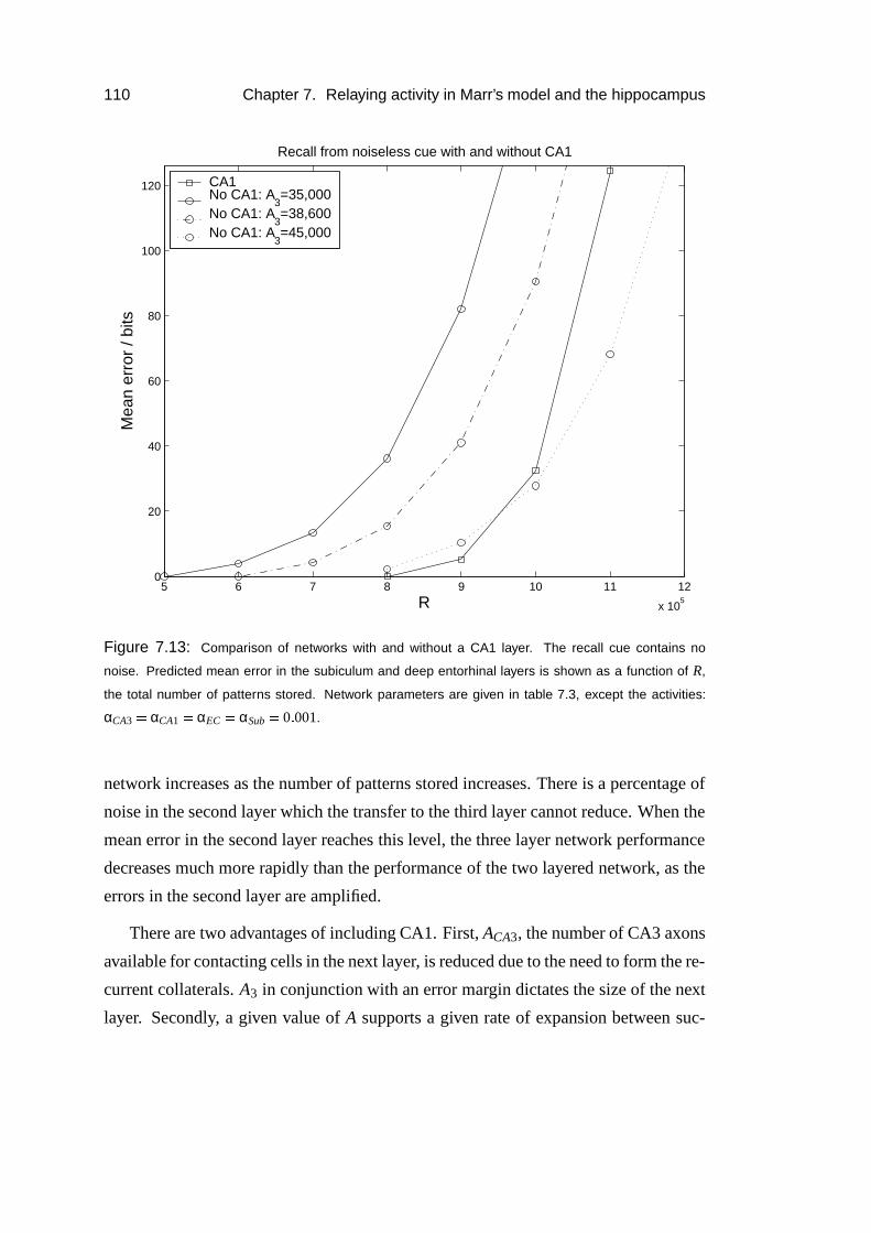
110 Chapter 7. Relaying activity in Marr’s model and the hippocampus
5 6 7 8 9 10 11 12
x 105
0
20
40
60
80
100
120
R
Mea
n er
ror
/ bits
Recall from noiseless cue with and without CA1
CA1No CA1: A
3=35,000
No CA1: A3=38,600
No CA1: A3=45,000
Figure 7.13: Comparison of networks with and without a CA1 layer. The recall cue contains no
noise. Predicted mean error in the subiculum and deep entorhinal layers is shown as a function of R,
the total number of patterns stored. Network parameters are given in table 7.3, except the activities:
αCA3 � αCA1 � αEC � αSub � 0 � 001.
network increases as the number of patterns stored increases. There is a percentage of
noise in the second layer which the transfer to the third layer cannot reduce. When the
mean error in the second layer reaches this level, the three layer network performance
decreases much more rapidly than the performance of the two layered network, as the
errors in the second layer are amplified.
There are two advantages of including CA1. First, ACA3, the number of CA3 axons
available for contacting cells in the next layer, is reduced due to the need to form the re-
current collaterals. A3 in conjunction with an error margin dictates the size of the next
layer. Secondly, a given value of A supports a given rate of expansion between suc-
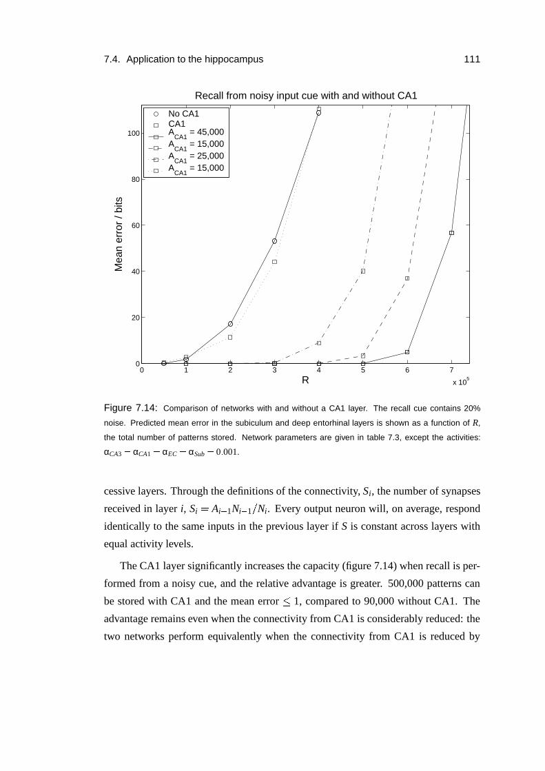
7.4. Application to the hippocampus 111
0 1 2 3 4 5 6 7
x 105
0
20
40
60
80
100
R
Mea
n er
ror
/ bits
Recall from noisy input cue with and without CA1
No CA1CA1A
CA1 = 45,000
ACA1
= 15,000A
CA1 = 25,000
ACA1
= 15,000
Figure 7.14: Comparison of networks with and without a CA1 layer. The recall cue contains 20%
noise. Predicted mean error in the subiculum and deep entorhinal layers is shown as a function of R,
the total number of patterns stored. Network parameters are given in table 7.3, except the activities:
αCA3 � αCA1 � αEC � αSub � 0 � 001.
cessive layers. Through the definitions of the connectivity, Si, the number of synapses
received in layer i, Si � Ai�
1Ni�
1 � Ni. Every output neuron will, on average, respond
identically to the same inputs in the previous layer if S is constant across layers with
equal activity levels.
The CA1 layer significantly increases the capacity (figure 7.14) when recall is per-
formed from a noisy cue, and the relative advantage is greater. 500,000 patterns can
be stored with CA1 and the mean error � 1, compared to 90,000 without CA1. The
advantage remains even when the connectivity from CA1 is considerably reduced: the
two networks perform equivalently when the connectivity from CA1 is reduced by
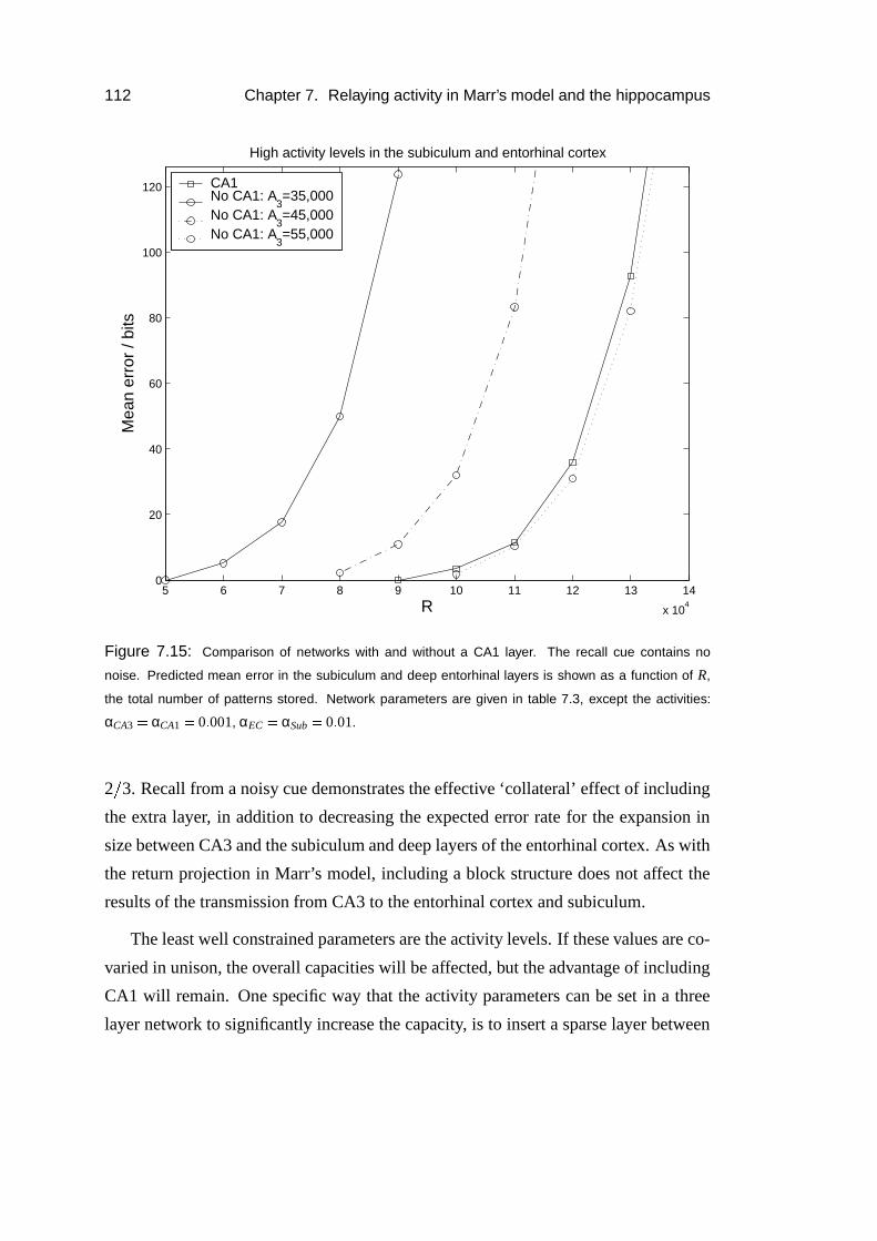
112 Chapter 7. Relaying activity in Marr’s model and the hippocampus
5 6 7 8 9 10 11 12 13 14
x 104
0
20
40
60
80
100
120
R
Mea
n er
ror
/ bits
High activity levels in the subiculum and entorhinal cortex
CA1No CA1: A
3=35,000
No CA1: A3=45,000
No CA1: A3=55,000
Figure 7.15: Comparison of networks with and without a CA1 layer. The recall cue contains no
noise. Predicted mean error in the subiculum and deep entorhinal layers is shown as a function of R,
the total number of patterns stored. Network parameters are given in table 7.3, except the activities:
αCA3 � αCA1 � 0 � 001, αEC � αSub � 0 � 01.
2 � 3. Recall from a noisy cue demonstrates the effective ‘collateral’ effect of including
the extra layer, in addition to decreasing the expected error rate for the expansion in
size between CA3 and the subiculum and deep layers of the entorhinal cortex. As with
the return projection in Marr’s model, including a block structure does not affect the
results of the transmission from CA3 to the entorhinal cortex and subiculum.
The least well constrained parameters are the activity levels. If these values are co-
varied in unison, the overall capacities will be affected, but the advantage of including
CA1 will remain. One specific way that the activity parameters can be set in a three
layer network to significantly increase the capacity, is to insert a sparse layer between

7.4. Application to the hippocampus 113
two highly active layers (discussed in Buckingham, 1991, section 6.2.2). Given the
computational demands on low activity levels in CA3, and the lack of any observable
difference in activity levels between CA3 and CA1, CA1 is highly unlikely to be per-
forming any such activity matching. As mentioned in the introduction to this section, it
is most likely that the activity levels in the entorhinal cortex and subiculum are higher
than in CA1 and CA3.
When the activity rates of the subiculum and entorhinal cortex are increased by
a factor of 10, the capacity in recall from a noiseless cue is significantly reduced for
both networks (figure 7.15). The advantage of including CA1 remains, and a greater
increase in A3 is required for the networks to perform equivalently.
7.4.3 Temporoammonic pathway
The contribution of the temporoammonic pathway has been ignored in considering
CA1 as a relay. Physiological evidence was presented in section 3.4 that the entorhinal-
CA1 forward and return projections operate as an independent reverberatory loop, via
the projection from the deep layers of the entorhinal cortex to superficial layers. It was
verified in section 7.3.7 that recurrently connecting a multilayered network increases
performance.
In this section, the entorhinal-CA1 reverberatory network is examined in the frame-
work of Marr’s model, to examine its suitability for the one-shot learning of associative
memories. The network is unlikely to perform pattern completion due to the limited
divergence of the forward and return projections. It could usefully perform noise re-
duction from full-sized cues. The spatial segregation of the parallel loops through
the entorhinal cortex and CA1 could maintain separate information streams (Longden
and Willshaw, 2002). Isolated information in these loops would be integrated in the
projections through the trisynaptic circuit.
Model parameters
The numbers of neurons in every layer of the network are given in table 7.4.3. It is
presumed that the majority of the synapses in the stratum lacunosum-moleculare of
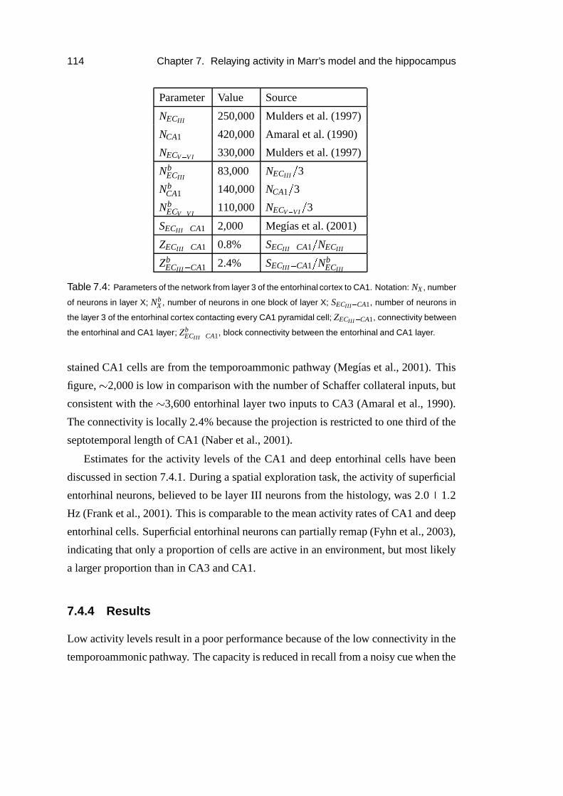
114 Chapter 7. Relaying activity in Marr’s model and the hippocampus
Parameter Value Source
NECIII 250,000 Mulders et al. (1997)
NCA1 420,000 Amaral et al. (1990)
NECV � V I 330,000 Mulders et al. (1997)
NbECIII
83,000 NECIII � 3
NbCA1 140,000 NCA1 � 3
NbECV � V I
110,000 NECV � VI � 3
SECIII�
CA1 2,000 Megıas et al. (2001)
ZECIII�
CA1 0.8% SECIII�
CA1 � NECIII
ZbECIII
�CA1 2.4% SECIII
�CA1 � Nb
ECIII
Table 7.4: Parameters of the network from layer 3 of the entorhinal cortex to CA1. Notation: NX , number
of neurons in layer X; NbX , number of neurons in one block of layer X; SECIII � CA1, number of neurons in
the layer 3 of the entorhinal cortex contacting every CA1 pyramidal cell; ZECIII � CA1, connectivity between
the entorhinal and CA1 layer; ZbECIII � CA1, block connectivity between the entorhinal and CA1 layer.
stained CA1 cells are from the temporoammonic pathway (Megıas et al., 2001). This
figure, � 2,000 is low in comparison with the number of Schaffer collateral inputs, but
consistent with the � 3,600 entorhinal layer two inputs to CA3 (Amaral et al., 1990).
The connectivity is locally 2 � 4% because the projection is restricted to one third of the
septotemporal length of CA1 (Naber et al., 2001).
Estimates for the activity levels of the CA1 and deep entorhinal cells have been
discussed in section 7.4.1. During a spatial exploration task, the activity of superficial
entorhinal neurons, believed to be layer III neurons from the histology, was 2 � 0�
1 � 2
Hz (Frank et al., 2001). This is comparable to the mean activity rates of CA1 and deep
entorhinal cells. Superficial entorhinal neurons can partially remap (Fyhn et al., 2003),
indicating that only a proportion of cells are active in an environment, but most likely
a larger proportion than in CA3 and CA1.
7.4.4 Results
Low activity levels result in a poor performance because of the low connectivity in the
temporoammonic pathway. The capacity is reduced in recall from a noisy cue when the
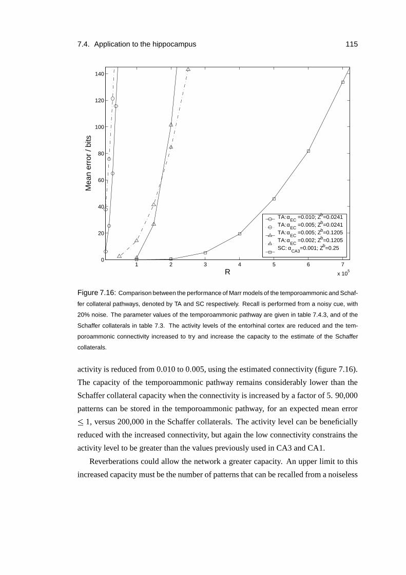
7.4. Application to the hippocampus 115
1 2 3 4 5 6 7
x 105
0
20
40
60
80
100
120
140
R
Mea
n er
ror
/ bits
TA: αEC
=0.010; Zb=0.0241TA: α
EC =0.005; Zb=0.0241
TA: αEC
=0.005; Zb=0.1205TA: α
EC =0.002; Zb=0.1205
SC: αCA3
=0.001; Zb=0.25
Figure 7.16: Comparison between the performance of Marr models of the temporoammonic and Schaf-
fer collateral pathways, denoted by TA and SC respectively. Recall is performed from a noisy cue, with
20% noise. The parameter values of the temporoammonic pathway are given in table 7.4.3, and of the
Schaffer collaterals in table 7.3. The activity levels of the entorhinal cortex are reduced and the tem-
poroammonic connectivity increased to try and increase the capacity to the estimate of the Schaffer
collaterals.
activity is reduced from 0 � 010 to 0 � 005, using the estimated connectivity (figure 7.16).
The capacity of the temporoammonic pathway remains considerably lower than the
Schaffer collateral capacity when the connectivity is increased by a factor of 5. 90,000
patterns can be stored in the temporoammonic pathway, for an expected mean error
� 1, versus 200,000 in the Schaffer collaterals. The activity level can be beneficially
reduced with the increased connectivity, but again the low connectivity constrains the
activity level to be greater than the values previously used in CA3 and CA1.
Reverberations could allow the network a greater capacity. An upper limit to this
increased capacity must be the number of patterns that can be recalled from a noiseless
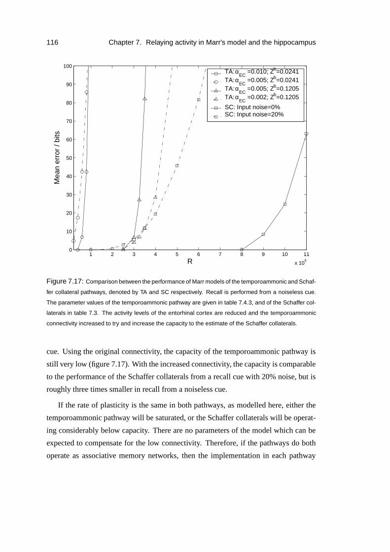
116 Chapter 7. Relaying activity in Marr’s model and the hippocampus
1 2 3 4 5 6 7 8 9 10 11
x 105
0
10
20
30
40
50
60
70
80
90
100
R
Mea
n er
ror
/ bits
TA: αEC
=0.010; Zb=0.0241TA: α
EC =0.005; Zb=0.0241
TA: αEC
=0.005; Zb=0.1205TA: α
EC =0.002; Zb=0.1205
SC: Input noise=0%SC: Input noise=20%
Figure 7.17: Comparison between the performance of Marr models of the temporoammonic and Schaf-
fer collateral pathways, denoted by TA and SC respectively. Recall is performed from a noiseless cue.
The parameter values of the temporoammonic pathway are given in table 7.4.3, and of the Schaffer col-
laterals in table 7.3. The activity levels of the entorhinal cortex are reduced and the temporoammonic
connectivity increased to try and increase the capacity to the estimate of the Schaffer collaterals.
cue. Using the original connectivity, the capacity of the temporoammonic pathway is
still very low (figure 7.17). With the increased connectivity, the capacity is comparable
to the performance of the Schaffer collaterals from a recall cue with 20% noise, but is
roughly three times smaller in recall from a noiseless cue.
If the rate of plasticity is the same in both pathways, as modelled here, either the
temporoammonic pathway will be saturated, or the Schaffer collaterals will be operat-
ing considerably below capacity. There are no parameters of the model which can be
expected to compensate for the low connectivity. Therefore, if the pathways do both
operate as associative memory networks, then the implementation in each pathway
7.5. Summary and discussion 117
must be different to avoid this capacity mismatch. One such implementation would
be when the rate of plasticity in the temporoammonic pathway is slower than in the
Schaffer collaterals.
7.5 Summary and discussion
In Marr’s model, suitably parameterised extra layers improve the performance in both
the forward and return projections. Any confusion over this result has stemmed from
attempting to constrain the connections at the network level, rather than from the cor-
rect perspective of every output neuron. In the forward projection, spatially organising
the connections into blocks improves performance because the cue can originate in an
isolated section of the neocortical layer. In the return projection, this block structur-
ing does not affect the performance as the recall cue is equally present throughout the
collateral layer.
The primary computational benefit of the extra layers is due to the limits of conver-
gence and divergence in neuron numbers between layers, that anatomically constrained
synaptic and axonal synapse numbers respectively can support. The secondary benefit,
for parameters sets operating further from the network capacity, is the collateral effect
of a recurrent network played out in a feedforward network.
The recent reports of plasticity in the pathways from CA1 to the subiculum and in
the deep layers of the entorhinal cortex (O’Mara et al., 2000; Yun et al., 2002) raise the
possibility that these precorticocortical pathways support the one-shot learning present
in CA3 (Nakazawa et al., 2003) and theoretically argued for in the Schaffer collaterals
(Treves, 1995). When Marr’s model is used to model the storage of associative mem-
ories between CA3, CA1 and the principal afferent targets of the hippocampus, the
subiculum and the entorhinal cortex, CA1 improves the capacity. This result provides
quantitative support for the idea of CA1 as a relay (Treves and Rolls, 1994).
The size of CA1 in the rat is well explained by the model. The combined size of
the deep entorhinal cortex layers and the subiculum is � 1.8 the size of CA3 (table 7.3).
The insertion of CA1 replaces this near doubling of neuron numbers with expansions of
1.3 between CA3 and CA1, and 1.4 between CA1 and the afferent target areas. These
118 Chapter 7. Relaying activity in Marr’s model and the hippocampus
smaller expansion ratios result in a greater capacity for a given error tolerance and
constrained number of axonal synapses, as was discussed in the results of section 7.4.1.
In contrast, the result does not explain neuron numbers in other species. In hu-
mans there are an estimated 2 � 7 � 106 neurons in CA3, 16 � 106 in CA1, 4 � 5 � 106
in the subiculum (West and Gundersen, 1990), and 3 � 8 � 106 neurons in layers V-VI
of the entorhinal cortex (West and Slomianka, 1998a,b). The number of CA1 neurons
amongst the 5 subjects varied considerably, from 11 to 24 � 106. If these numbers are
correct then the large number of CA1 neurons is not adequately explained by ensuring
successful transmission of information from CA3 to the rest of the brain.
Other anatomical aspects of CA1 in the rat remain unexplained, notably the spatial
organisations of the projections to and from CA1. The temporoammonic pathway is
topographically organised, such that to a first approximation, separate thirds of the sep-
totemporal length of the pathway are independent, and this organisation is maintained
throughout the subsequent projections between CA1, the subiculum and the entorhinal
cortex (Naber et al., 2001, see section 2.5). Within the framework of Marr’s model,
this striking organisation serves no purpose. It is possible that the connectivity is an
epiphenomenon, but perhaps unlikely.
The role for the temporoammonic input is not specified by (Treves and Rolls,
1994). The capacity of the entorhinal-CA1 Marr network as a Marr model is much
lower than that of the CA3-CA1 Marr network, over a broad parameter range. It is
therefore unlikely that both pathways operate as one-shot associative memory networks
which associate the same patterns of activity in CA1, (as proposed by Hasselmo and
Schnell, 1994).
The generality of the results gained by applying Marr’s model to the hippocampus
depend on the validity of the model’s simplifying assumptions. In the limit of sparse
coding, the assumption of binary synapses has little effect on the capacity of the net-
work to correctly retrieve patterns. In the Willshaw network (Willshaw et al., 1969),
when the original clipped binary Hebbian learning rule is replaced with an incremental
covariance Hebbian rule, the capacity of the network is reduced from 1/(2ln2) ( � 0.721)
bits per synapse to ln2 ( � 0.693) bits per synapse (Nadal and Toulouse, 1990). The ac-
curacy of the weight changes is not an important factor because sparse coding reduces
7.5. Summary and discussion 119
the interference between patterns.
Binary neurons can be considered to be a simplification of a binary rate-coding
scheme. In a recurrent network of threshold-linear neurons with covariance Hebbian
learning, the assumption of a binary distribution of rates has only a small effect on
the capacity (Treves and Rolls, 1991; Simmen et al., 1996). Again, this conclusion
is valid in the limit of sparse coding. The threshold-linear neuron model is a realistic
level of description in that it is able to reproduce the gross characteristics of the graded
response of a neuron to injected currents (Treves and Rolls, 1991). When the binary
rate-coding scheme in the network is replaced by a ternary or exponential distribution
of rates, the effect on the predicted capacity is small (Treves and Rolls, 1991, figure
6(a)).
The critical issue for determining how well the results generalise is the assumption
of sparse coding. The activity levels in the hippocampus are distinctively low (Barnes
et al., 1990). If the coding in the hippocampus is not sparse, then the capacity of the
network is significantly affected, and the fundamental assumption that the hippocam-
pus is an associative memory network has to be reexamined.

Chapter 8
Self-organising activity in Marr’s
model and the hippocampus
8.1 Introduction
How does the activity originate in every layer of Marr’s model? This is a relevant
problem for CA1 when the model is applied to the hippocampus. Excitatory connec-
tions allow input activity to autoassociate in CA3. Recurrent inhibitory connections
allow the dentate gyrus to operate as a competitive network. CA1 cannot rely upon
positive or negative feedback mechanisms to self-organise representations because it
lacks significant feedback connections (section 2.4).
Marr suggested an algorithm for pattern formation. The size of the input decides
whether or not a pattern is to be learnt or recalled. If it is below an activity level, it is
recalled, and if above, it is learnt (Marr, 1971, section 2.2.2). The aim is to choose the
most suitable cells to represent the current input when the pattern is learnt (Marr, 1971,
section 2.2.2). The chosen cells are the ones with the most active input synapses, the
highest input activity, a. The cells are connected by the so-called Brindley synapses
which have an unmodifiable excitatory component, regardless of whether the synapse
has been modified or not (Brindley, 1969). The Brindley synapses potentially allow
the output neurons with the highest input activity to be identified .
The algorithm is guided by a sensible principle, but omits important details. How
121
122 Chapter 8. Self-organising activity in Marr’s model and the hippocampus
does the output neuron sum the Brindley synapses without including the contribution
of the modified synapses? Neurons potentiated in one pattern will be more likely to be
active in the next. This problem is avoided by using a plasticity rule that ensures no net
weight gain. In this case, including the input activity in the dendritic sum biases the
neurons with the highest connectivity to be chosen. Unfortunately, Brindley synapses
are experimentally unsubstantiated. I discuss whether the NMDA component of Schaf-
fer collateral synapses could fulfil the same function at the end of this chapter. Marr
argues that his algorithm chooses the ‘best suited’ cells for representing the output, but
this is never qualified. Marr’s real motivation might have been biological plausibility:
if the position had been verified with private calculations, it is surprising that they were
not included in the paper.
Accurate analytic expressions were used to predict the performance of full-sized
hippocampal networks in the previous chapter. Buckingham (1991) extended the anal-
ysis to the network with self-organised patterns (appendix B), and used it to investigate
the performance of the ‘guess-s’ thresholding mechanism developed in the thesis. In
the guess-s mechanism, every output neuron adjusts its threshold to minimise its out-
put error. The estimate of the noise in the cue is gradually lowered across the network,
changing the threshold of the neuron (Buckingham and Willshaw, 1993). The guess-s
strategy was used to show that a self-organising network outperforms a competitive
network, proposed by Rolls (1989) to best describe the Schaffer collaterals (Bucking-
ham, 1991, section 5.4). Buckingham (1991) argued that networks storing random
and self-organised patterns perform equivalently. The reasoning was that the chosen
neurons have a higher connectivity, increasing performance, and have a higher propor-
tion of modified synapses, decreasing performance. This point is supported by a graph
of equivalent performances as a function of the noise in the cue (Buckingham, 1991,
figure 5.10).
Signal-to-noise analysis is used in this chapter to investigate the capacity of net-
works storing random or self-organised patterns. I show analytically that self-organising
networks have a higher capacity than networks storing random patterns with a higher
connectivity, in the arguably hippocampally relevant regime of low connectivity and a
high memory load, by considering the signal-to-noise ratio of the predicted dendritic
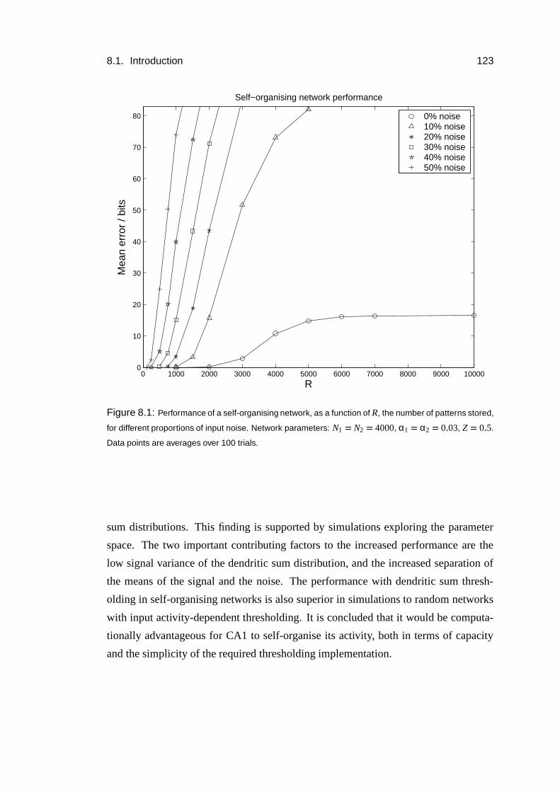
8.1. Introduction 123
0 1000 2000 3000 4000 5000 6000 7000 8000 9000 100000
10
20
30
40
50
60
70
80
R
Mea
n er
ror
/ bits
Self−organising network performance
0% noise10% noise20% noise30% noise40% noise50% noise
Figure 8.1: Performance of a self-organising network, as a function of R, the number of patterns stored,
for different proportions of input noise. Network parameters: N1 � N2 � 4000, α1 � α2 � 0 � 03, Z � 0 � 5.
Data points are averages over 100 trials.
sum distributions. This finding is supported by simulations exploring the parameter
space. The two important contributing factors to the increased performance are the
low signal variance of the dendritic sum distribution, and the increased separation of
the means of the signal and the noise. The performance with dendritic sum thresh-
olding in self-organising networks is also superior in simulations to random networks
with input activity-dependent thresholding. It is concluded that it would be computa-
tionally advantageous for CA1 to self-organise its activity, both in terms of capacity
and the simplicity of the required thresholding implementation.
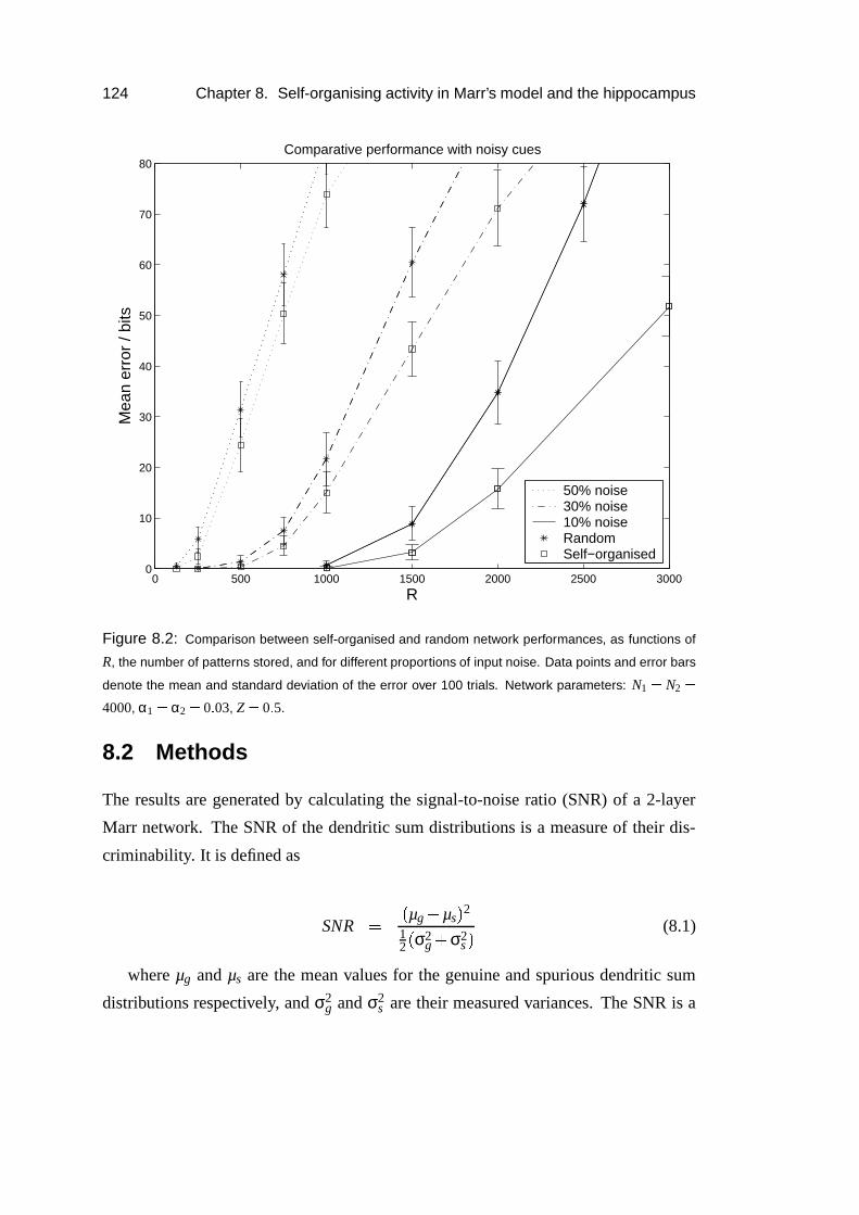
124 Chapter 8. Self-organising activity in Marr’s model and the hippocampus
0 500 1000 1500 2000 2500 30000
10
20
30
40
50
60
70
80
R
Mea
n er
ror
/ bits
Comparative performance with noisy cues
50% noise30% noise10% noiseRandomSelf−organised
Figure 8.2: Comparison between self-organised and random network performances, as functions of
R, the number of patterns stored, and for different proportions of input noise. Data points and error bars
denote the mean and standard deviation of the error over 100 trials. Network parameters: N1 � N2 �
4000, α1 � α2 � 0 � 03, Z � 0 � 5.
8.2 Methods
The results are generated by calculating the signal-to-noise ratio (SNR) of a 2-layer
Marr network. The SNR of the dendritic sum distributions is a measure of their dis-
criminability. It is defined as
SNR � � µg � µs � 212 � σ2
g� σ2
s � (8.1)
where µg and µs are the mean values for the genuine and spurious dendritic sum
distributions respectively, and σ2g and σ2
s are their measured variances. The SNR is a
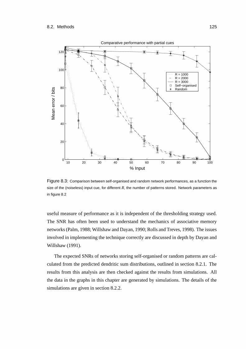
8.2. Methods 125
10 20 30 40 50 60 70 80 90 1000
20
40
60
80
100
120
% Input
Mea
n er
ror
/ bits
Comparative performance with partial cues
R = 1000R = 2000R = 3000Self−organisedRandom
Figure 8.3: Comparison between self-organised and random network performances, as a function the
size of the (noiseless) input cue, for different R, the number of patterns stored. Network parameters as
in figure 8.2
useful measure of performance as it is independent of the thresholding strategy used.
The SNR has often been used to understand the mechanics of associative memory
networks (Palm, 1988; Willshaw and Dayan, 1990; Rolls and Treves, 1998). The issues
involved in implementing the technique correctly are discussed in depth by Dayan and
Willshaw (1991).
The expected SNRs of networks storing self-organised or random patterns are cal-
culated from the predicted dendritic sum distributions, outlined in section 8.2.1. The
results from this analysis are then checked against the results from simulations. All
the data in the graphs in this chapter are generated by simulations. The details of the
simulations are given in section 8.2.2.
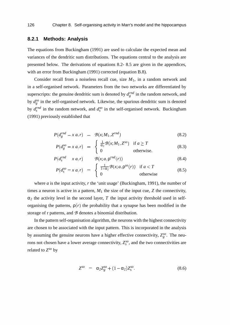
126 Chapter 8. Self-organising activity in Marr’s model and the hippocampus
8.2.1 Methods: Analysis
The equations from Buckingham (1991) are used to calculate the expected mean and
variances of the dendritic sum distributions. The equations central to the analysis are
presented below. The derivations of equations 8.2- 8.5 are given in the appendices,
with an error from Buckingham (1991) corrected (equation B.8).
Consider recall from a noiseless recall cue, size M1, in a random network and
in a self-organised network. Parameters from the two networks are differentiated by
superscripts: the genuine dendritic sum is denoted by drndg in the random network, and
by dsog in the self-organised network. Likewise, the spurious dendritic sum is denoted
by drnds in the random network, and dso
s in the self-organised network. Buckingham
(1991) previously established that
P � drndg � x
�a � r � � B � x;M1 � Zrnd � (8.2)
P � dsog � x
�a � r � �
�1
α2B � x;M1 � Zso � if a � T
0 otherwise �
(8.3)
P � drnds � x
�a � r � � B � x;a � ρrnd � r � � (8.4)
P � dsos � x
�a � r � �
�1
1�
α2B � x;a � ρso � r � � if a � T
0 otherwise(8.5)
where a is the input activity, r the ‘unit usage’ (Buckingham, 1991), the number of
times a neuron is active in a pattern, M1 the size of the input cue, Z the connectivity,
α2 the activity level in the second layer, T the input activity threshold used in self-
organising the patterns, ρ � r � the probability that a synapse has been modified in the
storage of r patterns, and B denotes a binomial distribution.
In the pattern self-organisation algorithm, the neurons with the highest connectivity
are chosen to be associated with the input pattern. This is incorporated in the analysis
by assuming the genuine neurons have a higher effective connectivity, Zsog . The neu-
rons not chosen have a lower average connectivity, Zsos , and the two connectivities are
related to Zso by
Zso � α2Zsog
� � 1 � α2 � Zsos � (8.6)
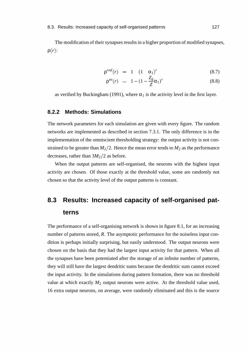
8.3. Results: Increased capacity of self-organised patterns 127
The modification of their synapses results in a higher proportion of modified synapses,
ρ � r � :
ρrnd � r � � 1 � � 1 � α1 � r (8.7)
ρso � r � � 1 � � 1 �
Zg
Zα1 � r (8.8)
as verified by Buckingham (1991), where α1 is the activity level in the first layer.
8.2.2 Methods: Simulations
The network parameters for each simulation are given with every figure. The random
networks are implemented as described in section 7.3.1. The only difference is in the
implementation of the omniscient thresholding strategy: the output activity is not con-
strained to be greater than M2 � 2. Hence the mean error tends to M2 as the performance
decreases, rather than 3M2 � 2 as before.
When the output patterns are self-organised, the neurons with the highest input
activity are chosen. Of those exactly at the threshold value, some are randomly not
chosen so that the activity level of the output patterns is constant.
8.3 Results: Increased capacity of self-organised pat-
terns
The performance of a self-organising network is shown in figure 8.1, for an increasing
number of patterns stored, R. The asymptotic performance for the noiseless input con-
dition is perhaps initially surprising, but easily understood. The output neurons were
chosen on the basis that they had the largest input activity for that pattern. When all
the synapses have been potentiated after the storage of an infinite number of patterns,
they will still have the largest dendritic sums because the dendritic sum cannot exceed
the input activity. In the simulations during pattern formation, there was no threshold
value at which exactly M2 output neurons were active. At the threshold value used,
16 extra output neurons, on average, were randomly eliminated and this is the source
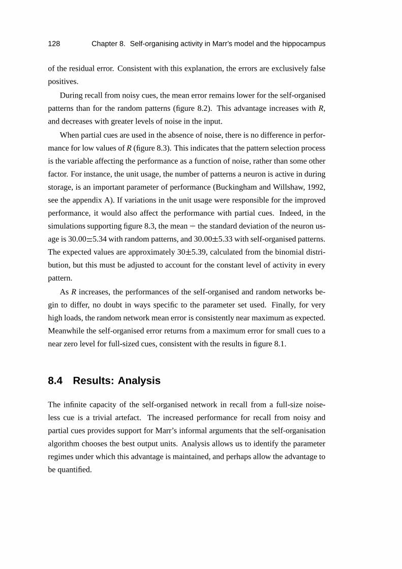
128 Chapter 8. Self-organising activity in Marr’s model and the hippocampus
of the residual error. Consistent with this explanation, the errors are exclusively false
positives.
During recall from noisy cues, the mean error remains lower for the self-organised
patterns than for the random patterns (figure 8.2). This advantage increases with R,
and decreases with greater levels of noise in the input.
When partial cues are used in the absence of noise, there is no difference in perfor-
mance for low values of R (figure 8.3). This indicates that the pattern selection process
is the variable affecting the performance as a function of noise, rather than some other
factor. For instance, the unit usage, the number of patterns a neuron is active in during
storage, is an important parameter of performance (Buckingham and Willshaw, 1992,
see the appendix A). If variations in the unit usage were responsible for the improved
performance, it would also affect the performance with partial cues. Indeed, in the
simulations supporting figure 8.3, the mean�
the standard deviation of the neuron us-
age is 30.00�
5.34 with random patterns, and 30.00�
5.33 with self-organised patterns.
The expected values are approximately 30�
5.39, calculated from the binomial distri-
bution, but this must be adjusted to account for the constant level of activity in every
pattern.
As R increases, the performances of the self-organised and random networks be-
gin to differ, no doubt in ways specific to the parameter set used. Finally, for very
high loads, the random network mean error is consistently near maximum as expected.
Meanwhile the self-organised error returns from a maximum error for small cues to a
near zero level for full-sized cues, consistent with the results in figure 8.1.
8.4 Results: Analysis
The infinite capacity of the self-organised network in recall from a full-size noise-
less cue is a trivial artefact. The increased performance for recall from noisy and
partial cues provides support for Marr’s informal arguments that the self-organisation
algorithm chooses the best output units. Analysis allows us to identify the parameter
regimes under which this advantage is maintained, and perhaps allow the advantage to
be quantified.
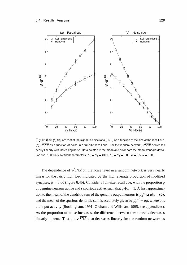
8.4. Results: Analysis 129
0 20 40 60 80 1000
1
2
3
4
5
6
7S
NR
1/2
% Input
(a) Partial cue
0 20 40 60 80 1000
1
2
3
4
5
6
7
% Noise
(a) Noisy cue
SN
R1/
2
Self−organisedRandom
Self−organisedRandom
Figure 8.4: (a) Square root of the signal-to-noise ratio (SNR) as a function of the size of the recall cue.
(b) � SNR as a function of noise in a full-size recall cue. For the random network, � SNR decreases
nearly linearly with increasing noise. Data points are the mean and error bars the mean standard devia-
tion over 100 trials. Network parameters: N1 � N2 � 4000, α1 � α2 � 0 � 03, Z � 0 � 5, R � 1000.
The dependence of � SNR on the noise level in a random network is very nearly
linear for the fairly high load indicated by the high average proportion of modified
synapses, ρ � 0 � 60 (figure 8.4b). Consider a full-size recall cue, with the proportion g
of genuine neurons active and s spurious active, such that g�
s � 1. A first approxima-
tion to the mean of the dendritic sum of the genuine output neurons is µrndg
� a � g �sρ � ,
and the mean of the spurious dendritic sum is accurately given by µrnds � aρ, where a is
the input activity (Buckingham, 1991; Graham and Willshaw, 1995, see appendices).
As the proportion of noise increases, the difference between these means decreases
linearly to zero. That the � SNR also decreases linearly for the random network as
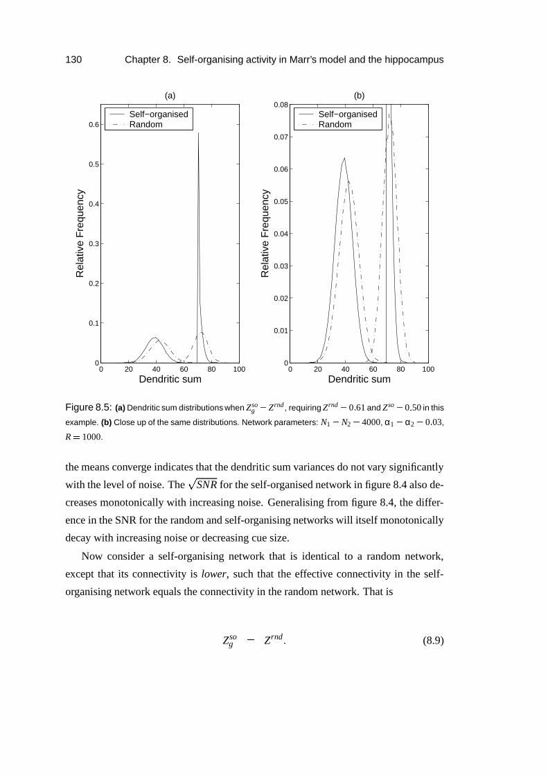
130 Chapter 8. Self-organising activity in Marr’s model and the hippocampus
0 20 40 60 80 1000
0.1
0.2
0.3
0.4
0.5
0.6
Dendritic sum
Rel
ativ
e F
requ
ency
(a)
0 20 40 60 80 1000
0.01
0.02
0.03
0.04
0.05
0.06
0.07
0.08
Rel
ativ
e F
requ
ency
Dendritic sum
(b)
Self−organisedRandom
Self−organisedRandom
Figure 8.5: (a) Dendritic sum distributions when Zsog � Zrnd , requiring Zrnd � 0 � 61 and Zso � 0 � 50 in this
example. (b) Close up of the same distributions. Network parameters: N1 � N2 � 4000, α1 � α2 � 0 � 03,
R � 1000.
the means converge indicates that the dendritic sum variances do not vary significantly
with the level of noise. The � SNR for the self-organised network in figure 8.4 also de-
creases monotonically with increasing noise. Generalising from figure 8.4, the differ-
ence in the SNR for the random and self-organising networks will itself monotonically
decay with increasing noise or decreasing cue size.
Now consider a self-organising network that is identical to a random network,
except that its connectivity is lower, such that the effective connectivity in the self-
organising network equals the connectivity in the random network. That is
Zsog � Zrnd
� (8.9)
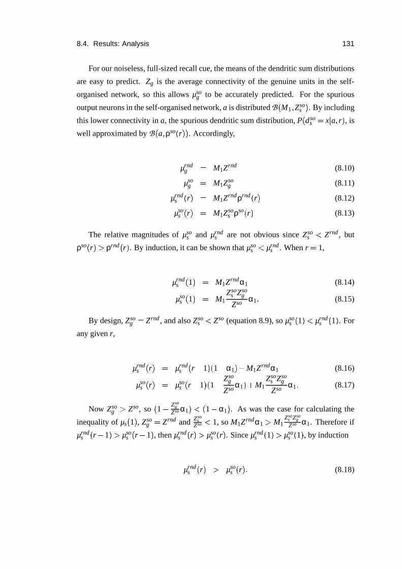
8.4. Results: Analysis 131
For our noiseless, full-sized recall cue, the means of the dendritic sum distributions
are easy to predict. Zg is the average connectivity of the genuine units in the self-
organised network, so this allows µsog to be accurately predicted. For the spurious
output neurons in the self-organised network, a is distributed B � M1 � Zsos � . By including
this lower connectivity in a, the spurious dendritic sum distribution, P � dsos � x
�a � r � , is
well approximated by B � a � ρso � r � � . Accordingly,
µrndg � M1Zrnd (8.10)
µsog � M1Zso
g (8.11)
µrnds � r � � M1Zrndρrnd � r � (8.12)
µsos � r � � M1Zso
s ρso � r � (8.13)
The relative magnitudes of µsos and µrnd
s are not obvious since Zsos � Zrnd , but
ρso � r � � ρrnd � r � . By induction, it can be shown that µsos � µrnd
s . When r � 1,
µrnds � 1 � � M1Zrndα1 (8.14)
µsos � 1 � � M1
Zsos Zso
g
Zso α1 � (8.15)
By design, Zsog � Zrnd , and also Zso
s � Zso (equation 8.9), so µsos � 1 � � µrnd
s � 1 � . For
any given r,
µrnds � r � � µrnd
s � r � 1 � � 1 � α1 � �M1Zrndα1 (8.16)
µsos � r � � µso
s � r � 1 � � 1 �
Zsog
Zso α1 � �M1
Zsos Zso
g
Zso α1 � (8.17)
Now Zsog � Zso, so � 1 �
Zsog
Zso α1 � � � 1 � α1 � . As was the case for calculating the
inequality of µs � 1 � , Zsog � Zrnd and Zso
sZso � 1, so M1Zrndα1 � M1
Zsos Zso
gZso α1. Therefore if
µrnds � r � 1 � � µso
s � r � 1 � , then µrnds � r � � µso
s � r � . Since µrnds � 1 � � µso
s � 1 � , by induction
µrnds � r � � µso
s � r � � (8.18)

132 Chapter 8. Self-organising activity in Marr’s model and the hippocampus
Indeed, as r � ∞, µrnds � M1Zrnd and µso
s � M1Zsos , so µrnd
s � ∞ � � µsos � ∞ � .
Since r is distributed identically for both the networks,
µrnds � µso
s � (8.19)
The variances require a little more attention. The variance of a genuine neuron’s
dendritic sum in the self-organised network is intuitively small, as the variance of the
upper tail of the input activity distribution must be less than across the whole distri-
bution. Indeed, the majority of genuine neurons have an input activity equal at the
threshold during selection. The dendritic sums from illustrative networks are shown in
figure 8.5. In this example, σsog is clearly very low. In general, the genuine dendritic
sum variance can be calculated explicitly:
� σrndg � 2 � M1Zrnd � 1 � Zrnd � � (8.20)
� σsog � 2 � 1
α2∑
a � TB � a;M1 � Zso � � a � M1Zso
g � 2 � (8.21)
The variances of the spurious dendritic sums are tricky to calculate analytically.
Calculating the propagation of σa and σr through B � a � ρ � r � � results in an unwieldy ex-
pression. Instead, I consider parameter ranges of ρ � r � and Z that constrain the relative
magnitudes of σrnds and σso
s .
The variance of the self-organised spurious dendritic sum is well approximated by
aρso � r � � 1 � ρso � r � � , since α2�
1. The random spurious variance is aρrnd � r � � 1 �
ρrnd � r � � . If the random network is operating with low output error rates and maximal
information efficiency, then ρrnd � 0 � 5 (Willshaw et al., 1969; Canning and Gardner,
1988). When ρrnd � r � � 0 � 5, ρrnd � r � � ρso � r � (equations 8.7 and 8.8), so for given
values of a,
σrnds � r �
a � � σsos � r �
a � when ρrnd � r � � 0 � 5 (8.22)
How does this inequality vary over the distribution of a? The input activities
are distributed binomially, B � M1 � Zsos � and B � M1 � Zrnd � , so the variances are σso
a �M1Zso
s � 1 � Zsos � and σrnd
a � M1Zrnd � 1 � Zrnd � . Since Zsos � Zrnd , when Zrnd � 0 � 5
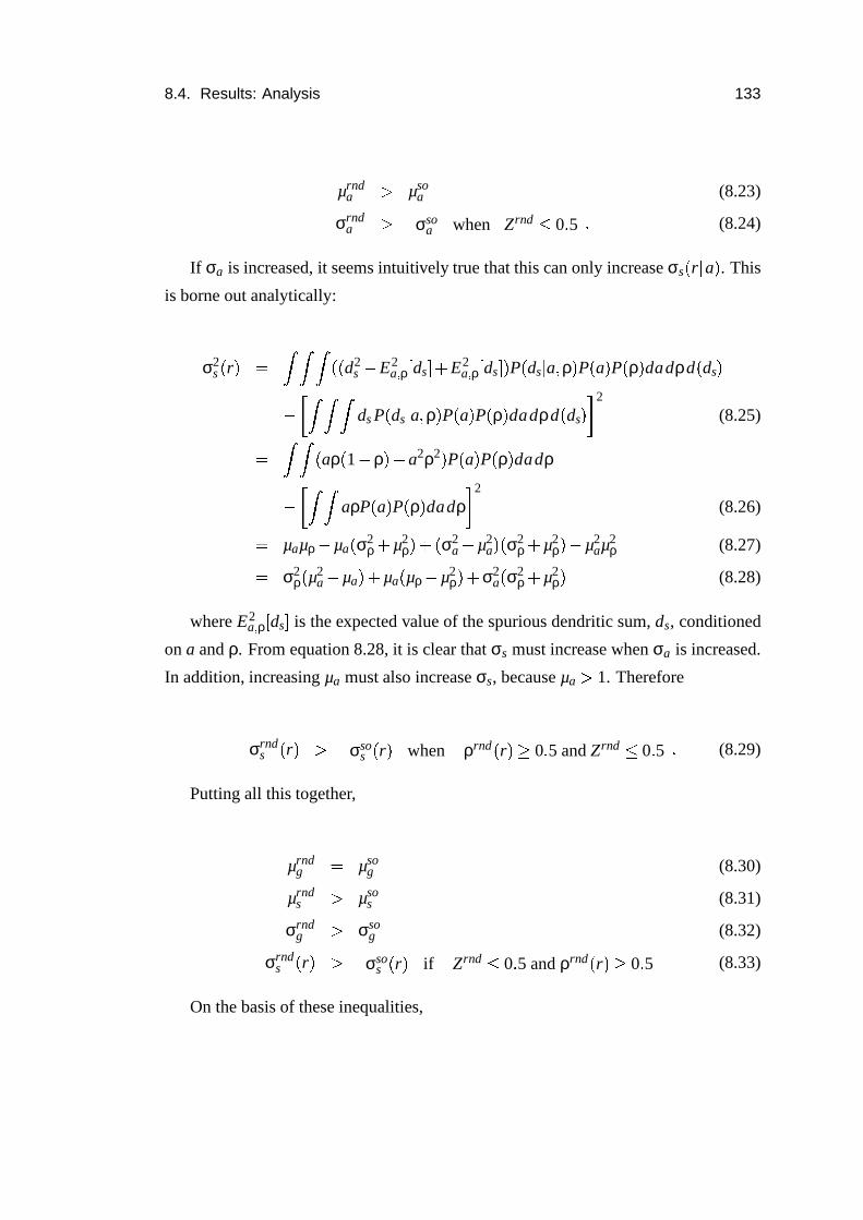
8.4. Results: Analysis 133
µrnda � µso
a (8.23)
σrnda � σso
a when Zrnd � 0 � 5 � (8.24)
If σa is increased, it seems intuitively true that this can only increase σs � r �a � . This
is borne out analytically:
σ2s � r � � �����
� � d2s � E2
a � ρ � ds � �E2
a � ρ � ds � � P � ds�a � ρ � P � a � P � ρ � dadρd � ds �
��� ����� ds P � ds�a � ρ � P � a � P � ρ � dadρd � ds ��� 2
(8.25)
� ���� aρ � 1 � ρ � �
a2ρ2 � P � a � P � ρ � dadρ
��� ��� aρP � a � P � ρ � dadρ � 2
(8.26)
� µaµρ � µa � σ2ρ
�µ2
ρ � � � σ2a
�µ2
a � � σ2ρ
�µ2
ρ � � µ2aµ2
ρ (8.27)
� σ2ρ � µ2
a � µa � �µa � µρ � µ2
ρ � � σ2a � σ2
ρ�
µ2ρ � (8.28)
where E2a � ρ � ds � is the expected value of the spurious dendritic sum, ds, conditioned
on a and ρ. From equation 8.28, it is clear that σs must increase when σa is increased.
In addition, increasing µa must also increase σs, because µa � 1. Therefore
σrnds � r � � σso
s � r � when ρrnd � r � � 0 � 5 and Zrnd � 0 � 5 � (8.29)
Putting all this together,
µrndg � µso
g (8.30)
µrnds � µso
s (8.31)
σrndg � σso
g (8.32)
σrnds � r � � σso
s � r � if Zrnd � 0 � 5 and ρrnd � r � � 0 � 5 (8.33)
On the basis of these inequalities,
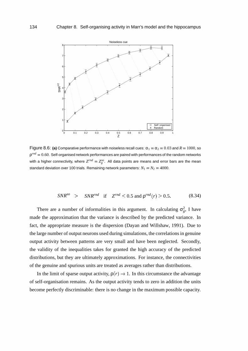
134 Chapter 8. Self-organising activity in Marr’s model and the hippocampus
0 0.1 0.2 0.3 0.4 0.5 0.6 0.7 0.8 0.9 10
1
2
3
4
5
6
7
8
SN
R1/
2
Noiseless cue
Z
Self−organisedRandom
Figure 8.6: (a) Comparative performance with noiseless recall cues: α1 � α2 � 0 � 03 and R � 1000, so
ρrnd � 0 � 60. Self-organised network performances are paired with performances of the random networks
with a higher connectivity, where Zrnd � Zsog . All data points are means and error bars are the mean
standard deviation over 100 trials. Remaining network parameters: N1 � N2 � 4000.
SNRso � SNRrnd if Zrnd � 0 � 5 and ρrnd � r � � 0 � 5 � (8.34)
There are a number of informalities in this argument. In calculating σ2g, I have
made the approximation that the variance is described by the predicted variance. In
fact, the appropriate measure is the dispersion (Dayan and Willshaw, 1991). Due to
the large number of output neurons used during simulations, the correlations in genuine
output activity between patterns are very small and have been neglected. Secondly,
the validity of the inequalities takes for granted the high accuracy of the predicted
distributions, but they are ultimately approximations. For instance, the connectivities
of the genuine and spurious units are treated as averages rather than distributions.
In the limit of sparse output activity, ρ � r � � 1. In this circumstance the advantage
of self-organisation remains. As the output activity tends to zero in addition the units
become perfectly discriminable: there is no change in the maximum possible capacity.
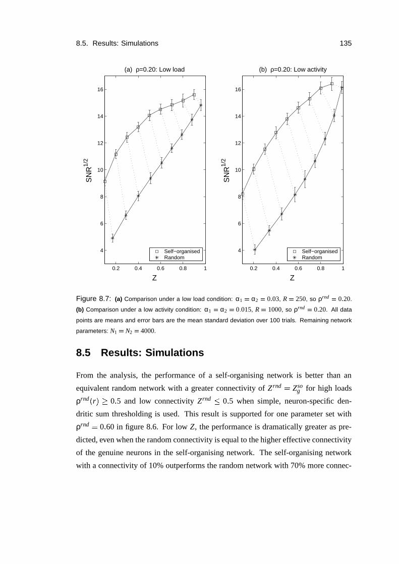
8.5. Results: Simulations 135
0.2 0.4 0.6 0.8 1
4
6
8
10
12
14
16
Z
SN
R1/
2
(a) ρ=0.20: Low load
0.2 0.4 0.6 0.8 1
4
6
8
10
12
14
16
Z
SN
R1/
2
(b) ρ=0.20: Low activity
Self−organisedRandom
Self−organisedRandom
Figure 8.7: (a) Comparison under a low load condition: α1 � α2 � 0 � 03, R � 250, so ρrnd � 0 � 20.
(b) Comparison under a low activity condition: α1 � α2 � 0 � 015, R � 1000, so ρrnd � 0 � 20. All data
points are means and error bars are the mean standard deviation over 100 trials. Remaining network
parameters: N1 � N2 � 4000.
8.5 Results: Simulations
From the analysis, the performance of a self-organising network is better than an
equivalent random network with a greater connectivity of Zrnd � Zsog for high loads
ρrnd � r � � 0 � 5 and low connectivity Zrnd � 0 � 5 when simple, neuron-specific den-
dritic sum thresholding is used. This result is supported for one parameter set with
ρrnd � 0 � 60 in figure 8.6. For low Z, the performance is dramatically greater as pre-
dicted, even when the random connectivity is equal to the higher effective connectivity
of the genuine neurons in the self-organising network. The self-organising network
with a connectivity of 10% outperforms the random network with 70% more connec-
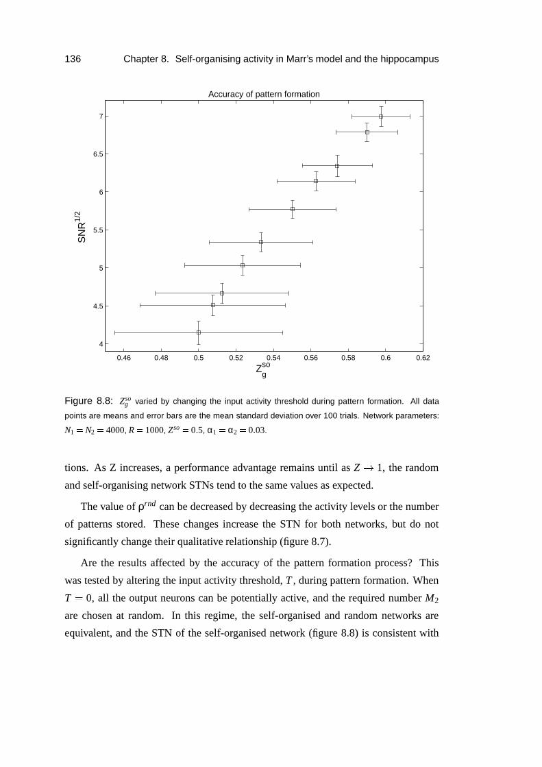
136 Chapter 8. Self-organising activity in Marr’s model and the hippocampus
0.46 0.48 0.5 0.52 0.54 0.56 0.58 0.6 0.62
4
4.5
5
5.5
6
6.5
7
Zgso
SN
R1/
2
Accuracy of pattern formation
Figure 8.8: Zsog varied by changing the input activity threshold during pattern formation. All data
points are means and error bars are the mean standard deviation over 100 trials. Network parameters:
N1 � N2 � 4000, R � 1000, Zso � 0 � 5, α1 � α2 � 0 � 03.
tions. As Z increases, a performance advantage remains until as Z � 1, the random
and self-organising network STNs tend to the same values as expected.
The value of ρrnd can be decreased by decreasing the activity levels or the number
of patterns stored. These changes increase the STN for both networks, but do not
significantly change their qualitative relationship (figure 8.7).
Are the results affected by the accuracy of the pattern formation process? This
was tested by altering the input activity threshold, T , during pattern formation. When
T � 0, all the output neurons can be potentially active, and the required number M2
are chosen at random. In this regime, the self-organised and random networks are
equivalent, and the STN of the self-organised network (figure 8.8) is consistent with
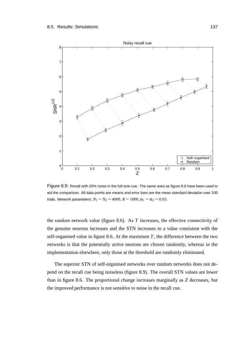
8.5. Results: Simulations 137
0 0.1 0.2 0.3 0.4 0.5 0.6 0.7 0.8 0.9 10
1
2
3
4
5
6
7
8
SN
R1/
2
Z
Noisy recall cue
Self−organisedRandom
Figure 8.9: Recall with 20% noise in the full-size cue. The same axes as figure 8.6 have been used to
aid the comparison. All data points are means and error bars are the mean standard deviation over 100
trials. Network parameters: N1 � N2 � 4000, R � 1000, α1 � α2 � 0 � 03.
the random network value (figure 8.6). As T increases, the effective connectivity of
the genuine neurons increases and the STN increases to a value consistent with the
self-organised value in figure 8.6. At the maximum T , the difference between the two
networks is that the potentially active neurons are chosen randomly, whereas in the
implementation elsewhere, only those at the threshold are randomly eliminated.
The superior STN of self-organised networks over random networks does not de-
pend on the recall cue being noiseless (figure 8.9). The overall STN values are lower
than in figure 8.6. The proportional change increases marginally as Z decreases, but
the improved performance is not sensitive to noise in the recall cue.
138 Chapter 8. Self-organising activity in Marr’s model and the hippocampus
8.6 Results: Thresholding dependence
In a binary associative memory network storing random patterns, partial connectivity
results in a distribution of input activities. Variations in the input activity to each cell
result increase the variance of the dendritic sum distribution. The capacity of the net-
work is significantly lower than is predicted when this effect is not taken into account
(Buckingham, 1991). Thresholding mechanisms have been proposed that improve the
network performance by reducing or compensating for variations in the input activity
distributions (Marr, 1971; Buckingham and Willshaw, 1993; Graham and Willshaw,
1995). However, none of these mechanisms has satisfactorily explained how the input
activity to each cell can be measured.
Marr (1971) uses an inhibitory cell to measure the input activity to each pyramidal
cell. This requires as many interneurons as pyramidal cells. This is unlikely because
only � 10% of hippocampal neurons are inhibitory interneurons (Freund and Buzsaki,
1996). Furthermore, the basket cells proposed to mediate the divisive inhibition con-
tact more than 1500 pyramidal cells (Sik et al., 1995). Buckingham and Willshaw
(1993) assume that the input activity is known. Graham and Willshaw (1995) propose
a scheme in which NMDARs communicate the dendritic sum and AMPA receptors
(AMPARs) communicate the input activity of the cell. The AMPA signal puts the cell
into a state such that the subsequent NMDA response is integrated to result in a somatic
potential equal to the dendritic sum divided by the input activity. This scheme is not
consistent with the large variation in the number of AMPA receptors and the relatively
low variation in the number of NMDA receptors in Schaffer collateral synapses (Racca
et al., 2000).
If input activity information is not available during recall, how can the effects of
partial connectivity on the capacity be reduced? In the self-organising network, there
is little variation in the input activity of the genuine neurons by design. Therefore a
divisive threshold will not improve the performance (figure 8.10). In this section, it is
shown in simulations that a self-organising network with a dendritic sum threshold out-
performs a random network with both an dendritic sum and an input activity threshold
of the omniscient thresholding strategy.
It should be noted that the omniscient strategy is not the optimal input activity-
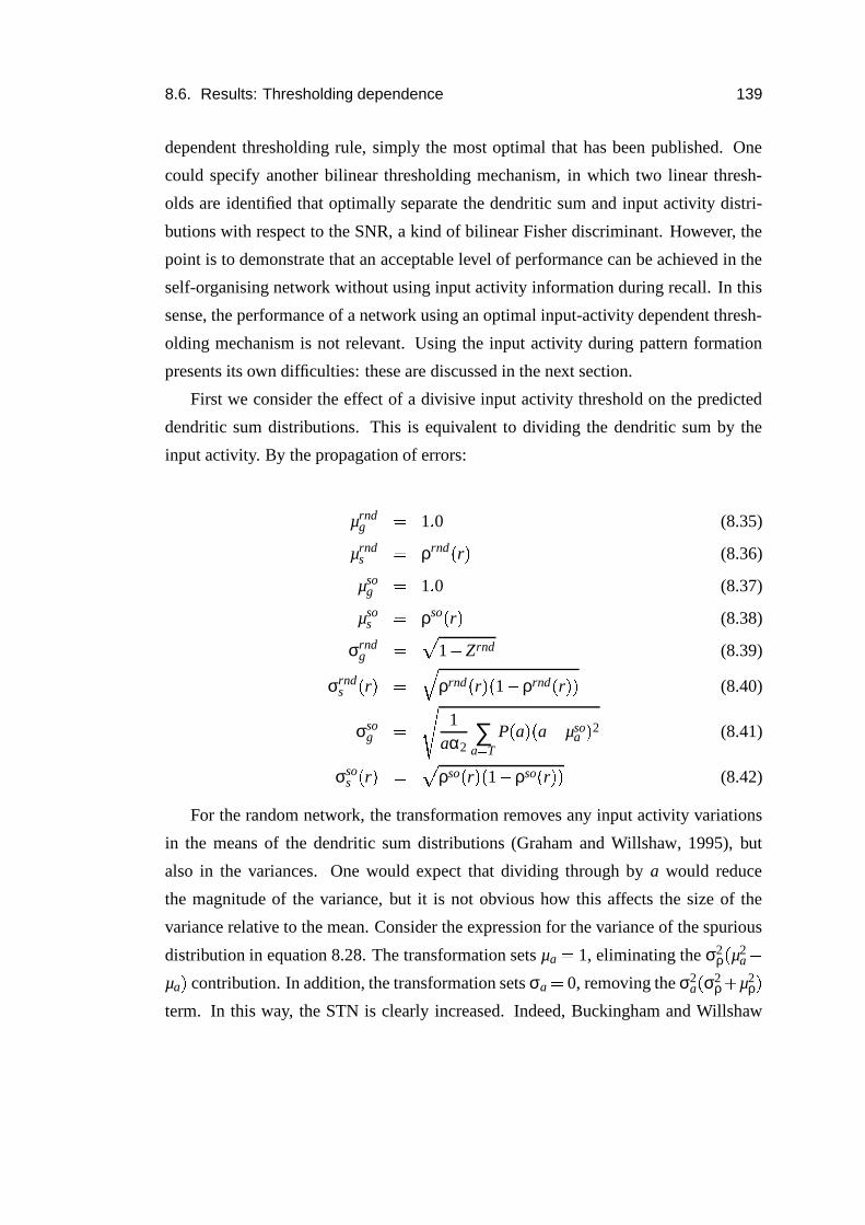
8.6. Results: Thresholding dependence 139
dependent thresholding rule, simply the most optimal that has been published. One
could specify another bilinear thresholding mechanism, in which two linear thresh-
olds are identified that optimally separate the dendritic sum and input activity distri-
butions with respect to the SNR, a kind of bilinear Fisher discriminant. However, the
point is to demonstrate that an acceptable level of performance can be achieved in the
self-organising network without using input activity information during recall. In this
sense, the performance of a network using an optimal input-activity dependent thresh-
olding mechanism is not relevant. Using the input activity during pattern formation
presents its own difficulties: these are discussed in the next section.
First we consider the effect of a divisive input activity threshold on the predicted
dendritic sum distributions. This is equivalent to dividing the dendritic sum by the
input activity. By the propagation of errors:
µrndg � 1 � 0 (8.35)
µrnds � ρrnd � r � (8.36)
µsog � 1 � 0 (8.37)
µsos � ρso � r � (8.38)
σrndg � � 1 � Zrnd (8.39)
σrnds � r � � � ρrnd � r � � 1 � ρrnd � r � � (8.40)
σsog � 1
aα2∑
a � TP � a � � a � µso
a � 2 (8.41)
σsos � r � � � ρso � r � � 1 � ρso � r � � (8.42)
For the random network, the transformation removes any input activity variations
in the means of the dendritic sum distributions (Graham and Willshaw, 1995), but
also in the variances. One would expect that dividing through by a would reduce
the magnitude of the variance, but it is not obvious how this affects the size of the
variance relative to the mean. Consider the expression for the variance of the spurious
distribution in equation 8.28. The transformation sets µa � 1, eliminating the σ2ρ � µ2
a �
µa � contribution. In addition, the transformation sets σa � 0, removing the σ2a � σ2
ρ�
µ2ρ �
term. In this way, the STN is clearly increased. Indeed, Buckingham and Willshaw
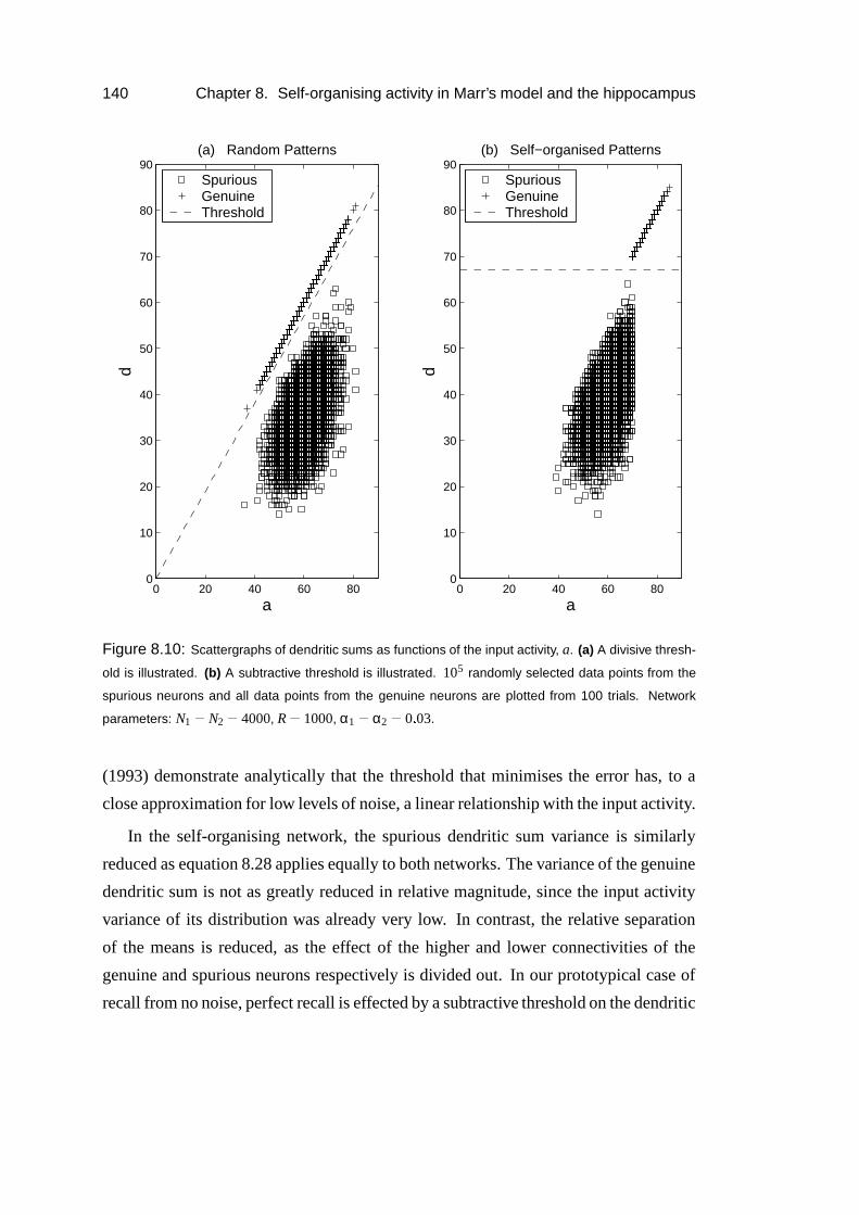
140 Chapter 8. Self-organising activity in Marr’s model and the hippocampus
0 20 40 60 800
10
20
30
40
50
60
70
80
90
a
d
(a) Random Patterns
0 20 40 60 800
10
20
30
40
50
60
70
80
90
d
(b) Self−organised Patterns
a
SpuriousGenuineThreshold
SpuriousGenuineThreshold
Figure 8.10: Scattergraphs of dendritic sums as functions of the input activity, a. (a) A divisive thresh-
old is illustrated. (b) A subtractive threshold is illustrated. 105 randomly selected data points from the
spurious neurons and all data points from the genuine neurons are plotted from 100 trials. Network
parameters: N1 � N2 � 4000, R � 1000, α1 � α2 � 0 � 03.
(1993) demonstrate analytically that the threshold that minimises the error has, to a
close approximation for low levels of noise, a linear relationship with the input activity.
In the self-organising network, the spurious dendritic sum variance is similarly
reduced as equation 8.28 applies equally to both networks. The variance of the genuine
dendritic sum is not as greatly reduced in relative magnitude, since the input activity
variance of its distribution was already very low. In contrast, the relative separation
of the means is reduced, as the effect of the higher and lower connectivities of the
genuine and spurious neurons respectively is divided out. In our prototypical case of
recall from no noise, perfect recall is effected by a subtractive threshold on the dendritic

8.6. Results: Thresholding dependence 141
0.1 0.2 0.3 0.4 0.5 0.6 0.7 0.8 0.9 12
3
4
5
6
7
8
Z
SN
R1/
2
Input activity−dependent thresholding
Self−organised (d/a)Self−organised (d)Random (d/a)Random (d)
Figure 8.11: The SNR calculated for the dendritic sum divided by the input activity (‘d/a’ in legend),
for recall from a noiseless cue. Data from figure 8.6 is plotted for comparison (‘d’ in legend). All data
points are means and error bars are the mean standard deviation over 100 trials. Network parameters:
N1 � N2 � 4000, R � 1000, α1 � α2 � 0 � 03.
sum, mimicking the conditions during pattern formation.
Implementing input activity-dependent thresholding greatly improves the STN of
the random network, as expected (figure 8.11). It also decreases the performance of the
self-organised network: the reduction in the difference between the means is greater
than the reduction in the spurious dendritic sum variance for this parameter set. It is
noteworthy that the STN of the random network with input activity thresholding is
consistently lower over the full between extrema range of connectivity. This is consis-
tent with the superior performance of the network in figures 8.2 and 8.3 during recall
with partial and noisy cues respectively.
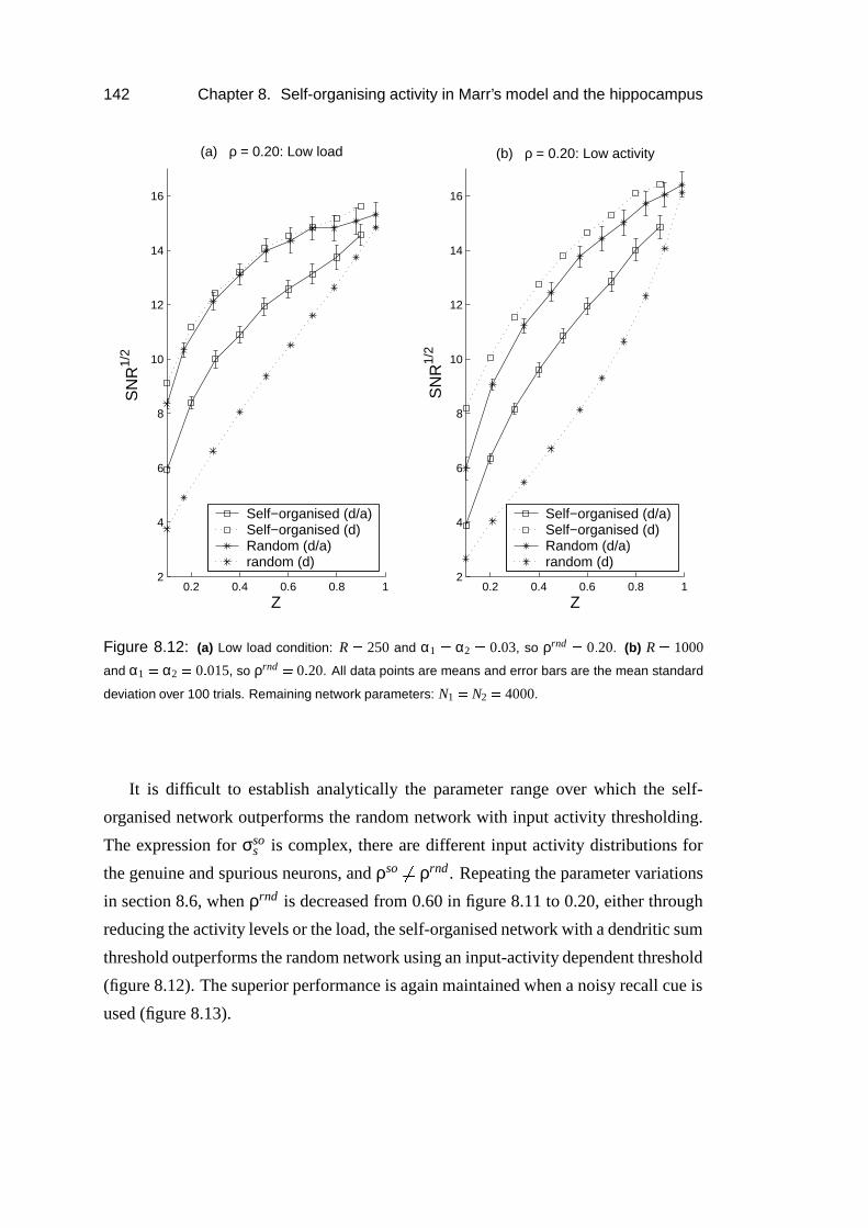
142 Chapter 8. Self-organising activity in Marr’s model and the hippocampus
0.2 0.4 0.6 0.8 12
4
6
8
10
12
14
16
SN
R1/
2
Z
(a) ρ = 0.20: Low load
0.2 0.4 0.6 0.8 12
4
6
8
10
12
14
16
SN
R1/
2
Z
(b) ρ = 0.20: Low activity
Self−organised (d/a)Self−organised (d)Random (d/a)random (d)
Self−organised (d/a)Self−organised (d)Random (d/a)random (d)
Figure 8.12: (a) Low load condition: R � 250 and α1 � α2 � 0 � 03, so ρrnd � 0 � 20. (b) R � 1000
and α1 � α2 � 0 � 015, so ρrnd � 0 � 20. All data points are means and error bars are the mean standard
deviation over 100 trials. Remaining network parameters: N1 � N2 � 4000.
It is difficult to establish analytically the parameter range over which the self-
organised network outperforms the random network with input activity thresholding.
The expression for σsos is complex, there are different input activity distributions for
the genuine and spurious neurons, and ρso �� ρrnd . Repeating the parameter variations
in section 8.6, when ρrnd is decreased from 0.60 in figure 8.11 to 0.20, either through
reducing the activity levels or the load, the self-organised network with a dendritic sum
threshold outperforms the random network using an input-activity dependent threshold
(figure 8.12). The superior performance is again maintained when a noisy recall cue is
used (figure 8.13).

8.7. Self-organising CA1 activity 143
0.1 0.2 0.3 0.4 0.5 0.6 0.7 0.8 0.9 11
1.5
2
2.5
3
3.5
4
4.5
5
5.5
6
Z
SN
R1/
2
Noisy recall cue
Self−organised (d/a)Self−organised (d)Random (d/a)Random (d)
Figure 8.13: Recall with 20% noise in the full-size cue. All data points are means and error bars
are the mean standard deviation over 100 trials. Network parameters: N1 � N2 � 4000, R � 1000,
α1 � α2 � 0 � 03.
8.7 Self-organising CA1 activity
There are at least three ways that CA1 activity can be formed, to be associated with in-
coming CA3 activity. The Schaffer collaterals could self-organise a pattern of activity
in CA1, using the algorithm suggested by Marr (1971). Secondly, the temporoam-
monic pathway could impose a pattern of activity on CA1 (e.g. McClelland and God-
dard, 1996). Finally, CA1 could operate as a competitive network, using mutual inhi-
bition to form CA1 activity (Rolls, 1989).
Marr’s pattern formation algorithm produces an analytically supported superior ca-
pacity in comparison with random networks, for low connectivities and high loads. Un-
der a preliminary parameter search, it also appears to provide better or equivalent per-
144 Chapter 8. Self-organising activity in Marr’s model and the hippocampus
formance to random networks that use the more complex and non-local input-activity
dependent thresholding mechanisms. The major remaining difficulty is its implemen-
tation. How can a neuron calculate its input activity during pattern formation? If it uses
Brindley synapses, there is no way for the output neuron to integrate the Brindley com-
ponent without also integrating the modified component of the synapse. Marr proposes
that feedback neurons compensate for the number of modified synapses, so that remov-
ing the inhibition that counteracts the Brindley component allows the input activity to
be calculated (Marr, 1971, section 4.3.2). This set-up would require multiple sets of
dedicated, specific inhibitory connections so far completely unsubstantiated. Finally,
there is no experimental support for Brindley synapses as originally envisioned.
If the temporoammonic inputs impose a pattern of activity in CA1, the result would,
at best, be random activity. The temporoammonic synaptic matrix will result in cor-
relations in activity transmitted to CA1 from hypothetical uncorrelated entorhinal pat-
terns of activity. In practice, entorhinal layer II and III patterns are highly correlated, in
comparison to hippocampal patterns of activity, when small adjustments are made to an
environment’s shape, floor texture and food type (Fyhn et al., 2003). It is possible that
the sparse temporoammonic connectivity, the increased size of CA1 and the observed
plasticity in the temporoammonic pathway (Remondes and Schuman, 2002) individu-
ally or collectively orthogonalise the entorhinal inputs. The occurrence of CA1 place
field activity with CA3 lesioned (Brun et al., 2002) indicates that this may be the case.
Preliminary reports of simultaneous recordings of entorhinal layer III and CA1 in CA3
lesioned rats indicate that entorhinal activity is indeed decorrelated in CA1 (Fyhn et al.,
2003). In the Marr or Willshaw networks, uncorrelated random patterns create consid-
erable demands on thresholding mechanisms to maintain a given level of performance
in comparison with patterns self-organised by Marr’s prescription. Correlated patterns
further decrease performance by increasing crosstalk.
CA1 is least likely to operate as a competitive network. There is a lack of recurrent
collaterals to implement strong feedback inhibition, as discussed in section 2.4. When
rats explore a novel environment, CA1 interneuron activity decreases (Nitz and Mc-
Naughton, 2004). It would be surprising if interneuron activity was crucial in the for-
mation of spatial memories during this period. Marr’s model applied to CA1 requires
8.7. Self-organising CA1 activity 145
some method of activity regulation, either to maintain an activity level or to minimise
the error. It is envisioned that CA3 performs recall, such that CA1 will receive full
or nearly full-size patterns with only a small amount of noise. Under these circum-
stances, the requirements to maintain activity levels do not require massive feedback
inhibition. In any case, the capacity of a competitive network, using lateral inhibition
or a plasticity rule, has an upper bound of the capacity of a corresponding associative
memory network.
In summary, were there to be a way for the network to implement the Marr al-
gorithm, it would be computationally beneficial. Marr self-organised networks have
a higher capacity than networks storing random patterns, and the latter have a higher
capacity than competitive networks, all other parameters being equal. Finally, at the
cost of an elaborate prior pattern selection algorithm, Marr self-organising networks
require a relatively simple and local implementation. Whilst binary networks exag-
gerate the importance of thresholding by simplifying the activity and synaptic weight
distributions, the issues remain in partially connected associative memory networks
with real valued activities and weights.
8.7.1 CA1 activity in novel environments
What happens during pattern formation in CA1? As discussed in section 4.2, neu-
rophysiological correlates of memories of single events are notoriously difficult to
identify, both conceptually and experimentally. Place fields are the most observable
patterns of hippocampal activity in the rat, and thought to be the substance of at least
spatial memory (discussed in Bures et al., 1997; Nakazawa et al., 2004). By observing
their formation, it is possible to examine one aspect of hippocampal memory forma-
tion.
During the exploration of a novel environment, CA1 pyramidal cell activity levels
are elevated (Wilson and McNaughton, 1993), and the activity levels of CA1 interneu-
rons targeting perisomatic and dendritic regions of pyramidal cells are decreased (Nitz
and McNaughton, 2004), as discussed in detail in section 4.3. What is the function of
the elevated CA1 pyramidal cell activity? Undoubtedly, it indicates an increased rate
of plastic change in the Schaffer collaterals (e.g. Li et al., 2003). This may associate
146 Chapter 8. Self-organising activity in Marr’s model and the hippocampus
CA3 activity with CA1 activity imposed by the temporoammonic pathway.
The altered physiology during place field formation could be indicative of an out-
put neuron selection process, independent of temporoammonic input. Attention, or
behavioural relevance, is required to form place fields with long-term stability (Ken-
tros et al., 2004), and dopamine is required to consolidate LTP (Frey and Morris, 1998).
During the exploration of a novel environment, there is a dopamine-dependent facili-
tation of LTP induction (Li et al., 2003) and dopamine blocks temporoammonic trans-
mission in the slice (Otmakhova and Lisman, 2000).
8.7.2 Brindley synapses reconsidered
The Schaffer collaterals synapses invariably contain NMDARs. In contrast, the distri-
bution of the number of AMPARs per synapse is much broader, including numerous
‘silent synapses’, synapses with no AMPA component (Isaac et al., 1995). In one study
focussing on the stratum radiatum, fewer than 1% of glutamatergic synapses did not
contain NMDARs, but 12% did not contain AMPARs (Racca et al., 2000). In the same
study, the skewness of the distribution of the number of NMDARs per synapse was
half that for AMPARs.
A CA1 pyramidal cell depolarised through lower inhibition, including dendritic
inhibition, can therefore receive two signals in response to brief Schaffer collateral
stimulation. The first is a fast AMPA response, a function of the number of potentiated
synapses. The second is a slower NMDA response, a function of the input activity.
This is a speculative mechanism by which the selection of output neurons, chosen by
virtue of their high dendritic sum input, will be biased towards those with a high input
activity.
Consistent with this idea is data from the expression of the c-fos gene, which im-
ages neuronal activity mainly through calcium influx, during the first 30 minutes of
the exploration of a novel environment (Hess et al., 1995). CA1 activity increased by
a factor of between 3 and 4, whilst CA3 activity increased by a factor of 2. Calcium
levels do not map simply to activity levels, but this level of c-fos activity is roughly
8 times greater than the 43% excitatory activity increase observed by Nitz and Mc-
Naughton (2004). This relatively large influx of calcium could equally be explained
8.8. Summary and discussion 147
by the increased back propagation of action potentials, a large source of calcium influx
in CA1 pyramidal cells (Spruston et al., 1995).
The feasibility of the idea rests on the timescale of the dendritic integration. NMDAR-
mediated EPSCs have a rise time of � 10 ms, an order of magnitude longer than the
AMPA EPSCs. The time course of the change in output response to a change in the in-
put activity distribution is governed by the synaptic time constant (Treves, 1993). Sim-
ulations or analysis are required to demonstrate whether a slower NMDAR-mediated
signalling of the input activity would in fact bias the choice of output units to those
with a higher input activity in simple models. The answer is not straightforward, since,
for instance NMDARs have a considerably higher affinity to glutamate than AMPARs
(Hille, 2001).
8.8 Summary and discussion
Marr (1971) proposed an algorithm for an associative memory network to self-organise
its output patterns during storage. The chosen output neurons have the highest connec-
tivity to the active input neurons, for every pattern. The resulting network is trivially
able to relay an infinite number of stored patterns, with a very low error (figure 8.1).
This boundary condition means that the performance is better than a network that has
stored randomly chosen patterns at high capacities, whether the cue is noisy (figure 8.2)
or incomplete (figure 8.3), in a general sense.
The superior performance is supported analytically using signal-to-noise analy-
sis, in the case where dendritic sum thresholding is used. Using very accurate, but
ultimately approximate expressions for the dendritic sums (Buckingham, 1991, see
appendices), it is demonstrated that the signal-to-noise ratio for the self-organised net-
work has to be greater than the random network for low connectivities (Z � 50%) and
high loads (probability of a synapse being modified, ρ � 0 � 5) in the random network.
Further, this is true even when the connectivity in the self-organising network is less
than the random network connectivity, such that only the neurons chosen to be active
in an output pattern have a connectivity (for that pattern) equal to the connectivity in
the random network. This result is verified in simulations, and an exploration of the
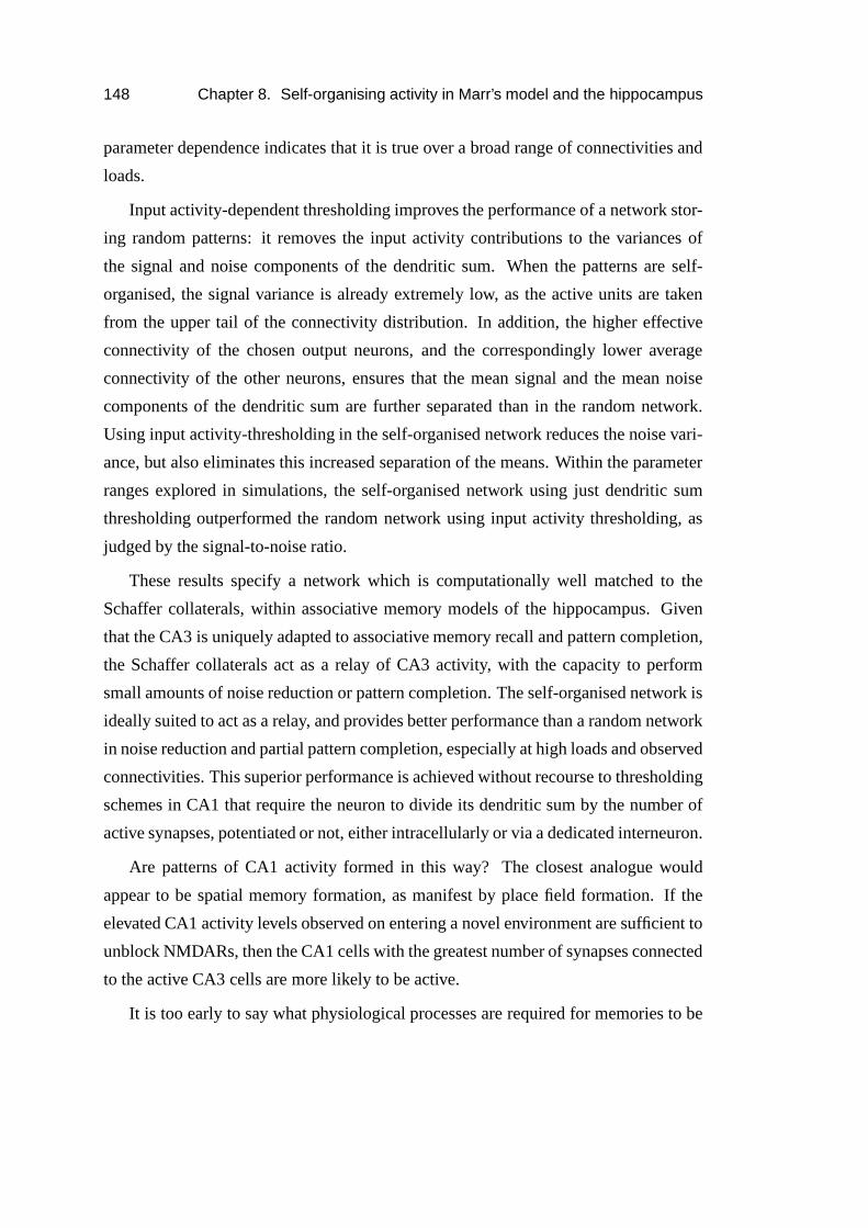
148 Chapter 8. Self-organising activity in Marr’s model and the hippocampus
parameter dependence indicates that it is true over a broad range of connectivities and
loads.
Input activity-dependent thresholding improves the performance of a network stor-
ing random patterns: it removes the input activity contributions to the variances of
the signal and noise components of the dendritic sum. When the patterns are self-
organised, the signal variance is already extremely low, as the active units are taken
from the upper tail of the connectivity distribution. In addition, the higher effective
connectivity of the chosen output neurons, and the correspondingly lower average
connectivity of the other neurons, ensures that the mean signal and the mean noise
components of the dendritic sum are further separated than in the random network.
Using input activity-thresholding in the self-organised network reduces the noise vari-
ance, but also eliminates this increased separation of the means. Within the parameter
ranges explored in simulations, the self-organised network using just dendritic sum
thresholding outperformed the random network using input activity thresholding, as
judged by the signal-to-noise ratio.
These results specify a network which is computationally well matched to the
Schaffer collaterals, within associative memory models of the hippocampus. Given
that the CA3 is uniquely adapted to associative memory recall and pattern completion,
the Schaffer collaterals act as a relay of CA3 activity, with the capacity to perform
small amounts of noise reduction or pattern completion. The self-organised network is
ideally suited to act as a relay, and provides better performance than a random network
in noise reduction and partial pattern completion, especially at high loads and observed
connectivities. This superior performance is achieved without recourse to thresholding
schemes in CA1 that require the neuron to divide its dendritic sum by the number of
active synapses, potentiated or not, either intracellularly or via a dedicated interneuron.
Are patterns of CA1 activity formed in this way? The closest analogue would
appear to be spatial memory formation, as manifest by place field formation. If the
elevated CA1 activity levels observed on entering a novel environment are sufficient to
unblock NMDARs, then the CA1 cells with the greatest number of synapses connected
to the active CA3 cells are more likely to be active.
It is too early to say what physiological processes are required for memories to be
8.8. Summary and discussion 149
stored. A leading theory is that attended events are automatically stored, whereas unat-
tended events are not (Morris and Frey, 1997). For instance, place fields formed by rats
attending to the environment are stable over days, whereas place fields formed in unat-
tended environments are not stable for more than 6 hours (Kentros et al., 2004). When
behaviourally relevant elements of the environment are discovered to have moved, such
as the hidden escape platform in a water maze, the physiological correlates are remark-
ably similar to those during the exploration of a novel environment: elevated pyrami-
dal cell activity, and reduced inhibitory cell activity (Fyhn et al., 2002). This activity
is only observed, however, in a proportion of cells, not across the population.
A soft application of Marr’s pattern self-organisation algorithm would involve the
short term potentiation of the Schaffer collateral synapses to some fraction of the CA1
cells best connected to the active CA3 cells, on entering the novel environment. Again,
this could be achieved through NMDAR activation. Of these cells, temporoammonic
input could choose which will be active. As illustrated in figure 8.8, the computational
advantages of self-organised patterns is not highly dependent on the accuracy of the
pattern formation process.

Chapter 9
Place field formation in the
temporoammonic pathway
9.1 Introduction
The place cell activity recorded without input from CA3 by Brun et al. (2002) provides
an exciting opportunity to examine the computational function of the temporoammonic
pathway. Numerous electrophysiological studies have established the inhibitory nature
of the pathway in the rat (Colbert and Levy, 1992; Empson and Heinemann, 1995;
Soltesz, 1995; Levy et al., 1995; Buzsaki et al., 1995; Leung, 1995, section 3.2). In
the absence of any significant excitatory somatic response, how can temporoammonic
input result in any kind of activity? I shall show that in an integrate-and-fire neu-
ron model of the pathway, when the entorhino-CA1 pyramidal cell EPSPs are assigned
long time constants, consistent with NMDARs, the response to synchronous slice stim-
ulation is inhibitory. The model pyramidal cells are still functionally active because
they are sensitive to increases in rate without increases in temporal correlation.
Most models of place field formation have used excitatory recurrent collaterals or
n-winners-take-all dynamics to convert entorhinal input into hippocampal place fields
(section 6). The low number of recurrent collaterals mean that these are unlikely mech-
anisms for generating narrow place fields in CA1 (section 2.4). Feedback inhibition
can be expected to refine the place field activity, but is not a striking feature of CA1. All
151
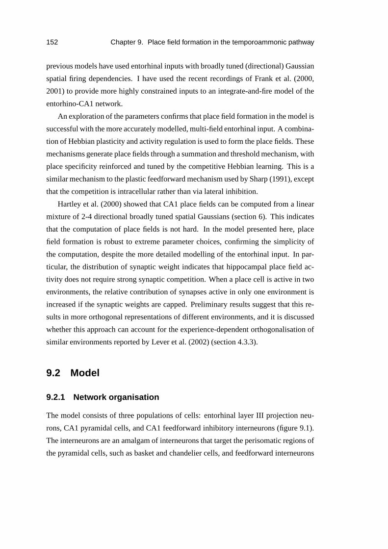
152 Chapter 9. Place field formation in the temporoammonic pathway
previous models have used entorhinal inputs with broadly tuned (directional) Gaussian
spatial firing dependencies. I have used the recent recordings of Frank et al. (2000,
2001) to provide more highly constrained inputs to an integrate-and-fire model of the
entorhino-CA1 network.
An exploration of the parameters confirms that place field formation in the model is
successful with the more accurately modelled, multi-field entorhinal input. A combina-
tion of Hebbian plasticity and activity regulation is used to form the place fields. These
mechanisms generate place fields through a summation and threshold mechanism, with
place specificity reinforced and tuned by the competitive Hebbian learning. This is a
similar mechanism to the plastic feedforward mechanism used by Sharp (1991), except
that the competition is intracellular rather than via lateral inhibition.
Hartley et al. (2000) showed that CA1 place fields can be computed from a linear
mixture of 2-4 directional broadly tuned spatial Gaussians (section 6). This indicates
that the computation of place fields is not hard. In the model presented here, place
field formation is robust to extreme parameter choices, confirming the simplicity of
the computation, despite the more detailed modelling of the entorhinal input. In par-
ticular, the distribution of synaptic weight indicates that hippocampal place field ac-
tivity does not require strong synaptic competition. When a place cell is active in two
environments, the relative contribution of synapses active in only one environment is
increased if the synaptic weights are capped. Preliminary results suggest that this re-
sults in more orthogonal representations of different environments, and it is discussed
whether this approach can account for the experience-dependent orthogonalisation of
similar environments reported by Lever et al. (2002) (section 4.3.3).
9.2 Model
9.2.1 Network organisation
The model consists of three populations of cells: entorhinal layer III projection neu-
rons, CA1 pyramidal cells, and CA1 feedforward inhibitory interneurons (figure 9.1).
The interneurons are an amalgam of interneurons that target the perisomatic regions of
the pyramidal cells, such as basket and chandelier cells, and feedforward interneurons
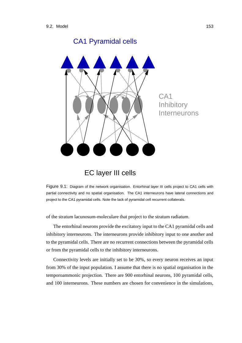
9.2. Model 153
CA1 Pyramidal cells
EC layer III cells
CA1InhibitoryInterneurons
Figure 9.1: Diagram of the network organisation. Entorhinal layer III cells project to CA1 cells with
partial connectivity and no spatial organisation. The CA1 interneurons have lateral connections and
project to the CA1 pyramidal cells. Note the lack of pyramidal cell recurrent collaterals.
of the stratum lacunosum-moleculare that project to the stratum radiatum.
The entorhinal neurons provide the excitatory input to the CA1 pyramidal cells and
inhibitory interneurons. The interneurons provide inhibitory input to one another and
to the pyramidal cells. There are no recurrent connections between the pyramidal cells
or from the pyramidal cells to the inhibitory interneurons.
Connectivity levels are initially set to be 30%, so every neuron receives an input
from 30% of the input population. I assume that there is no spatial organisation in the
temporoammonic projection. There are 900 entorhinal neurons, 100 pyramidal cells,
and 100 interneurons. These numbers are chosen for convenience in the simulations,
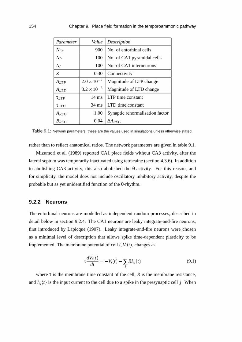
154 Chapter 9. Place field formation in the temporoammonic pathway
Parameter Value Description
NEc 900 No. of entorhinal cells
NP 100 No. of CA1 pyramidal cells
NI 100 No. of CA1 interneurons
Z 0.30 Connectivity
ALTP 2 � 0 � 10�
2 Magnitude of LTP change
ALTD 8 � 2 � 10�
3 Magnitude of LTD change
τLTP 14 ms LTP time constant
τLTD 34 ms LTD time constant
AREG 1.00 Synaptic renormalisation factor
BREG 0.04 ∆AREG
Table 9.1: Network parameters. these are the values used in simulations unless otherwise stated.
rather than to reflect anatomical ratios. The network parameters are given in table 9.1.
Mizumori et al. (1989) reported CA1 place fields without CA3 activity, after the
lateral septum was temporarily inactivated using tetracaine (section 4.3.6). In addition
to abolishing CA3 activity, this also abolished the θ-activity. For this reason, and
for simplicity, the model does not include oscillatory inhibitory activity, despite the
probable but as yet unidentified function of the θ-rhythm.
9.2.2 Neurons
The entorhinal neurons are modelled as independent random processes, described in
detail below in section 9.2.4. The CA1 neurons are leaky integrate-and-fire neurons,
first introduced by Lapicque (1907). Leaky integrate-and-fire neurons were chosen
as a minimal level of description that allows spike time-dependent plasticity to be
implemented. The membrane potential of cell i, Vi � t � , changes as
τdVi � t �
dt � � Vi � t � � ∑j
RIi j � t � (9.1)
where τ is the membrane time constant of the cell, R is the membrane resistance,
and Ii j � t � is the input current to the cell due to a spike in the presynaptic cell j. When
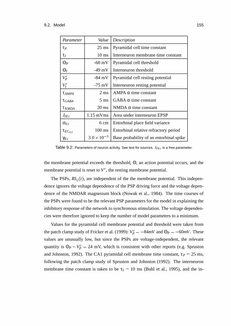
9.2. Model 155
Parameter Value Description
τP 25 ms Pyramidal cell time constant
τI 10 ms Interneuron membrane time constant
ΘP -60 mV Pyramidal cell threshold
ΘI -49 mV Interneuron threshold
V rP -84 mV Pyramidal cell resting potential
V rI -75 mV Interneuron resting potential
τAMPA 2 ms AMPA α time constant
τGABA 5 ms GABA α time constant
τNMDA 20 ms NMDA α time constant
JIEc 1.15 mVms Area under interneuron EPSP
σEc 6 cm Entorhinal place field variance
τECre f 100 ms Entorhinal relative refractory period
γEc 3 � 0 � 10�
3 Base probability of an entorhinal spike
Table 9.2: Parameters of neuron activity. See text for sources. JPEc is a free parameter.
the membrane potential exceeds the threshold, Θ, an action potential occurs, and the
membrane potential is reset to V r, the resting membrane potential.
The PSPs, RIi j � t � , are independent of the the membrane potential. This indepen-
dence ignores the voltage dependence of the PSP driving force and the voltage depen-
dence of the NMDAR magnesium block (Nowak et al., 1984). The time courses of
the PSPs were found to be the relevant PSP parameters for the model in explaining the
inhibitory response of the network to synchronous stimulation. The voltage dependen-
cies were therefore ignored to keep the number of model parameters to a minimum.
Values for the pyramidal cell membrane potential and threshold were taken from
the patch clamp study of Fricker et al. (1999): V rP � � 84mV and ΘP � � 60mV . These
values are unusually low, but since the PSPs are voltage-independent, the relevant
quantity is ΘP � V rP � 24 mV, which is consistent with other reports (e.g. Spruston
and Johnston, 1992). The CA1 pyramidal cell membrane time constant, τP � 25 ms,
following the patch clamp study of Spruston and Johnston (1992). The interneuron
membrane time constant is taken to be τI � 10 ms (Buhl et al., 1995), and the in-
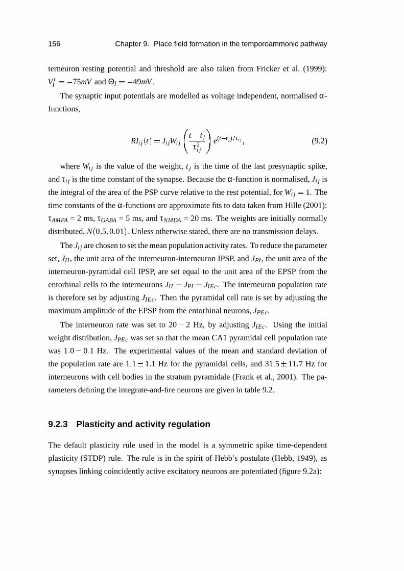
156 Chapter 9. Place field formation in the temporoammonic pathway
terneuron resting potential and threshold are also taken from Fricker et al. (1999):
V rI � � 75mV and ΘI � � 49mV .
The synaptic input potentials are modelled as voltage independent, normalised α-
functions,
RIi j � t � � Ji jWi j
�t � t j
τ2i j � e
�t�
t j � � τi j � (9.2)
where Wi j is the value of the weight, t j is the time of the last presynaptic spike,
and τi j is the time constant of the synapse. Because the α-function is normalised, Ji j is
the integral of the area of the PSP curve relative to the rest potential, for Wi j � 1. The
time constants of the α-functions are approximate fits to data taken from Hille (2001):
τAMPA = 2 ms, τGABA = 5 ms, and τNMDA = 20 ms. The weights are initially normally
distributed, N � 0 � 5 � 0 � 01 � . Unless otherwise stated, there are no transmission delays.
The Ji j are chosen to set the mean population activity rates. To reduce the parameter
set, JII, the unit area of the interneuron-interneuron IPSP, and JPI, the unit area of the
interneuron-pyramidal cell IPSP, are set equal to the unit area of the EPSP from the
entorhinal cells to the interneurons JII � JPI � JIEc. The interneuron population rate
is therefore set by adjusting JIEc. Then the pyramidal cell rate is set by adjusting the
maximum amplitude of the EPSP from the entorhinal neurons, JPEc.
The interneuron rate was set to 20�
2 Hz, by adjusting JIEc. Using the initial
weight distribution, JPEc was set so that the mean CA1 pyramidal cell population rate
was 1 � 0�
0 � 1 Hz. The experimental values of the mean and standard deviation of
the population rate are 1 � 1�
1 � 1 Hz for the pyramidal cells, and 31 � 5�
11 � 7 Hz for
interneurons with cell bodies in the stratum pyramidale (Frank et al., 2001). The pa-
rameters defining the integrate-and-fire neurons are given in table 9.2.
9.2.3 Plasticity and activity regulation
The default plasticity rule used in the model is a symmetric spike time-dependent
plasticity (STDP) rule. The rule is in the spirit of Hebb’s postulate (Hebb, 1949), as
synapses linking coincidently active excitatory neurons are potentiated (figure 9.2a):
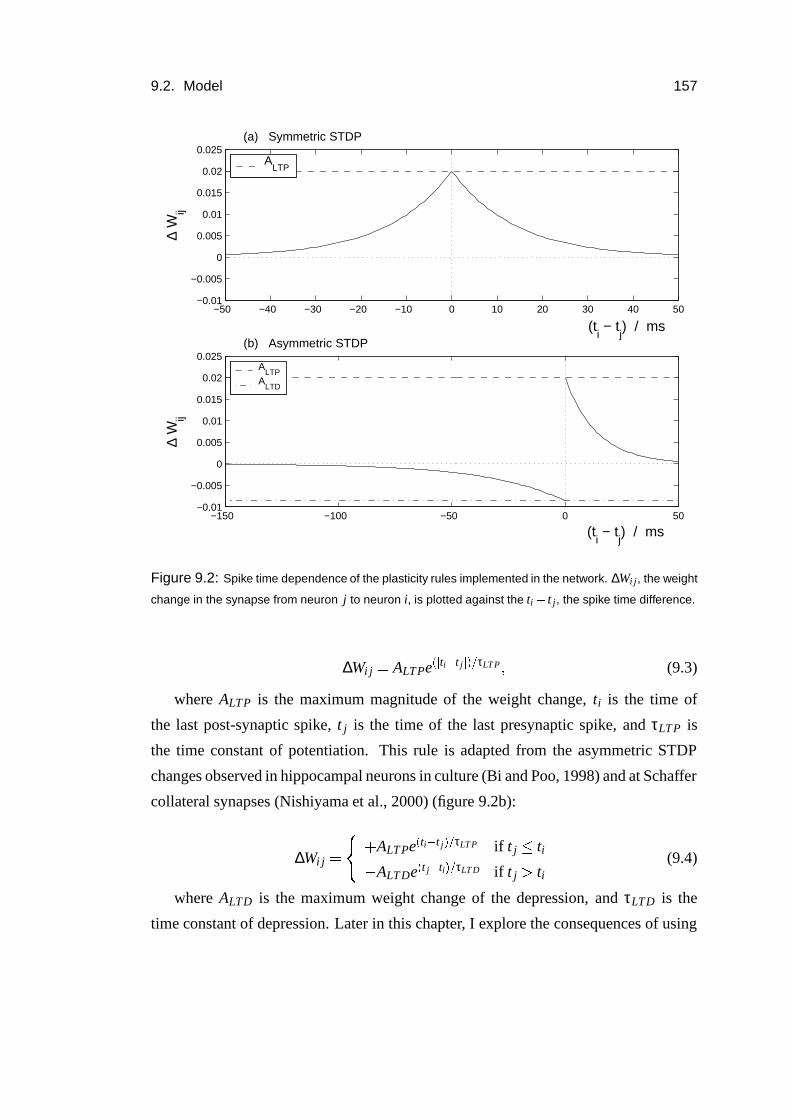
9.2. Model 157
−150 −100 −50 0 50−0.01
−0.005
0
0.005
0.01
0.015
0.02
0.025
(ti − t
j) / ms
∆ W
ij
(b) Asymmetric STDP
−50 −40 −30 −20 −10 0 10 20 30 40 50−0.01
−0.005
0
0.005
0.01
0.015
0.02
0.025
∆ W
ij
(a) Symmetric STDP
(ti − t
j) / ms
ALTP
ALTD
ALTP
Figure 9.2: Spike time dependence of the plasticity rules implemented in the network. ∆Wi j, the weight
change in the synapse from neuron j to neuron i, is plotted against the ti � t j, the spike time difference.
∆Wi j � ALTPe���
ti�
t j� � � τLT P � (9.3)
where ALTP is the maximum magnitude of the weight change, ti is the time of
the last post-synaptic spike, t j is the time of the last presynaptic spike, and τLTP is
the time constant of potentiation. This rule is adapted from the asymmetric STDP
changes observed in hippocampal neurons in culture (Bi and Poo, 1998) and at Schaffer
collateral synapses (Nishiyama et al., 2000) (figure 9.2b):
∆Wi j ��
�ALTPe
�ti�
t j � � τLT P if t j � ti
� ALTDe�t j
�ti � � τLT D if t j � ti
(9.4)
where ALTD is the maximum weight change of the depression, and τLTD is the
time constant of depression. Later in this chapter, I explore the consequences of using
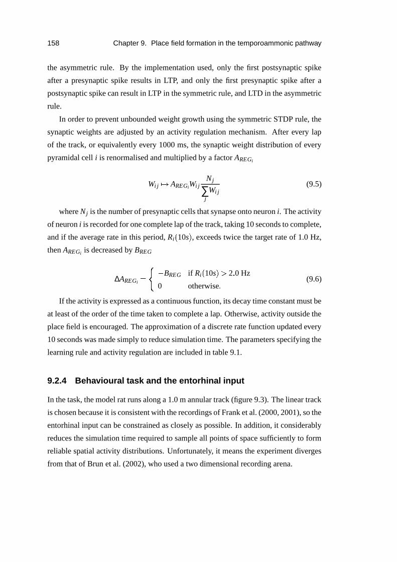
158 Chapter 9. Place field formation in the temporoammonic pathway
the asymmetric rule. By the implementation used, only the first postsynaptic spike
after a presynaptic spike results in LTP, and only the first presynaptic spike after a
postsynaptic spike can result in LTP in the symmetric rule, and LTD in the asymmetric
rule.
In order to prevent unbounded weight growth using the symmetric STDP rule, the
synaptic weights are adjusted by an activity regulation mechanism. After every lap
of the track, or equivalently every 1000 ms, the synaptic weight distribution of every
pyramidal cell i is renormalised and multiplied by a factor AREGi
Wi j �� AREGiWi jN j
∑j
Wi j(9.5)
where N j is the number of presynaptic cells that synapse onto neuron i. The activity
of neuron i is recorded for one complete lap of the track, taking 10 seconds to complete,
and if the average rate in this period, Ri � 10s � , exceeds twice the target rate of 1.0 Hz,
then AREGi is decreased by BREG
∆AREGi ��
� BREG if Ri � 10s � � 2 � 0 Hz
0 otherwise �
(9.6)
If the activity is expressed as a continuous function, its decay time constant must be
at least of the order of the time taken to complete a lap. Otherwise, activity outside the
place field is encouraged. The approximation of a discrete rate function updated every
10 seconds was made simply to reduce simulation time. The parameters specifying the
learning rule and activity regulation are included in table 9.1.
9.2.4 Behavioural task and the entorhinal input
In the task, the model rat runs along a 1.0 m annular track (figure 9.3). The linear track
is chosen because it is consistent with the recordings of Frank et al. (2000, 2001), so the
entorhinal input can be constrained as closely as possible. In addition, it considerably
reduces the simulation time required to sample all points of space sufficiently to form
reliable spatial activity distributions. Unfortunately, it means the experiment diverges
from that of Brun et al. (2002), who used a two dimensional recording arena.
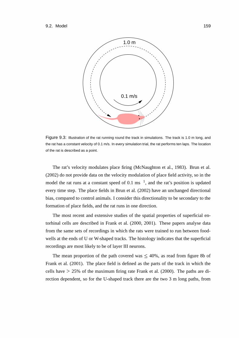
9.2. Model 159
0.1 m/s
1.0 m
Figure 9.3: Illustration of the rat running round the track in simulations. The track is 1.0 m long, and
the rat has a constant velocity of 0.1 m/s. In every simulation trial, the rat performs ten laps. The location
of the rat is described as a point.
The rat’s velocity modulates place firing (McNaughton et al., 1983). Brun et al.
(2002) do not provide data on the velocity modulation of place field activity, so in the
model the rat runs at a constant speed of 0.1 ms�
1, and the rat’s position is updated
every time step. The place fields in Brun et al. (2002) have an unchanged directional
bias, compared to control animals. I consider this directionality to be secondary to the
formation of place fields, and the rat runs in one direction.
The most recent and extensive studies of the spatial properties of superficial en-
torhinal cells are described in Frank et al. (2000, 2001). These papers analyse data
from the same sets of recordings in which the rats were trained to run between food-
wells at the ends of U or W-shaped tracks. The histology indicates that the superficial
recordings are most likely to be of layer III neurons.
The mean proportion of the path covered was � 40%, as read from figure 8b of
Frank et al. (2001). The place field is defined as the parts of the track in which the
cells have � 25% of the maximum firing rate Frank et al. (2000). The paths are di-
rection dependent, so for the U-shaped track there are the two 3 m long paths, from
160 Chapter 9. Place field formation in the temporoammonic pathway
EC place field
EC cells
Figure 9.4: An example of a random entorhinal cell’s place field location on the track.
the foodwell at one end to the foodwell at the other end, and back again. Along all
paths, the mean field length is � 70 cm, as read from figure 3a of Frank et al. (2000)
(calculated from the same data as Frank et al. (2001)). From this I have inferred that
every superficial entorhinal cell has, on average, two place fields covering 40% of the
track in one direction (figures 9.4 and 9.5).
Individual superficial entorhinal cells appear to fire independently. In 13 putative
excitatory cell pairs, there was no significant short time (1-3 ms) cross-correlation
(Frank et al., 2001). A lack of a peak in the cross-correlogram is consistent with inde-
pendent firing, but is not sufficient to prove it, since cross-correlograms ignore higher
order correlations than spike pairs and assume the neurons are in stationary states. For
36 superficial cells, the mean positional information was 0.46�
0.26 bits per spike
(Frank et al., 2000, figure 3b), implying that the cells fire fairly regularly, regardless of
the rat’s location. This is also reflected by the interspike interval distribution, which
peaks between 30 ms and 100 ms (Frank et al., 2001). In contrast, the interspike inter-
val distribution of CA1 pyramidal neurons has peaks�
10 ms and at � 125 ms.
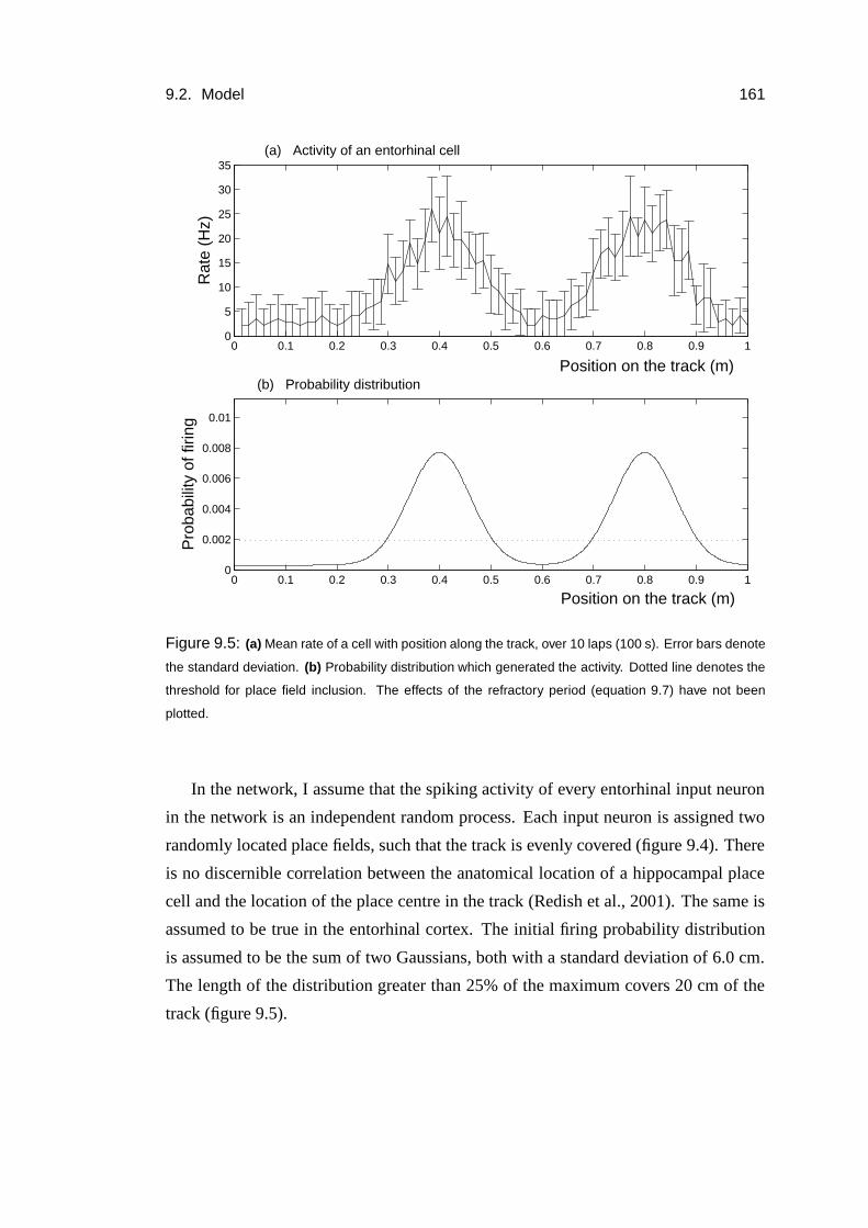
9.2. Model 161
0 0.1 0.2 0.3 0.4 0.5 0.6 0.7 0.8 0.9 10
5
10
15
20
25
30
35
Position on the track (m)
Rat
e (H
z)
(a) Activity of an entorhinal cell
0 0.1 0.2 0.3 0.4 0.5 0.6 0.7 0.8 0.9 10
0.002
0.004
0.006
0.008
0.01
Position on the track (m)
Pro
babi
lity
of fi
ring
(b) Probability distribution
Figure 9.5: (a) Mean rate of a cell with position along the track, over 10 laps (100 s). Error bars denote
the standard deviation. (b) Probability distribution which generated the activity. Dotted line denotes the
threshold for place field inclusion. The effects of the refractory period (equation 9.7) have not been
plotted.
In the network, I assume that the spiking activity of every entorhinal input neuron
in the network is an independent random process. Each input neuron is assigned two
randomly located place fields, such that the track is evenly covered (figure 9.4). There
is no discernible correlation between the anatomical location of a hippocampal place
cell and the location of the place centre in the track (Redish et al., 2001). The same is
assumed to be true in the entorhinal cortex. The initial firing probability distribution
is assumed to be the sum of two Gaussians, both with a standard deviation of 6.0 cm.
The length of the distribution greater than 25% of the maximum covers 20 cm of the
track (figure 9.5).
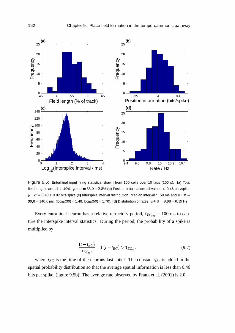
162 Chapter 9. Place field formation in the temporoammonic pathway
0.35 0.4 0.450
5
10
15
20
25
Position information (bits/spike)
Fre
quen
cy
(b)
45 50 55 60 650
5
10
15
20
25
Field length (% of track)
Fre
quen
cy
(a)
0 1 2 3 40
20
40
60
80
100
120
140
Log10
(Interspike interval / ms)
Fre
quen
cy
(c)
9.4 9.6 9.8 10 10.2 10.40
5
10
15
20
25
Rate / Hz
Fre
quen
cy
(d)
Figure 9.6: Entorhinal input firing statistics, drawn from 100 cells over 10 laps (100 s). (a) Total
field lengths are all � 40%. µ � σ � 55 � 0 � 2 � 8% (b) Position information: all values � 0.46 bits/spike.
µ � σ � 0 � 40 � 0 � 02 bits/spike (c) Interspike interval distribution. Median interval � 50 ms and µ � σ �
99 � 8 � 140 � 0 ms, (log10(30) = 1.48, log10(50) = 1.70). (d) Distribution of rates: µ � σ � 9 � 98 � 0 � 19 Hz
Every entorhinal neuron has a relative refractory period, τECre f = 100 ms to cap-
ture the interspike interval statistics. During the period, the probability of a spike is
multiplied by
� t � tEC �τECre f
if � t � tEC � � τECre f (9.7)
where tEC is the time of the neurons last spike. The constant γEc is added to the
spatial probability distribution so that the average spatial information is less than 0.46
bits per spike, (figure 9.5b). The average rate observed by Frank et al. (2001) is 2.0�
9.2. Model 163
1.2 Hz. The activity rate of the entorhinal cells in the model is set to 10�
1 Hz so that
every pyramidal cell receives enough inputs in my network. The parameters used to
define the entorhinal input are included in table 9.2.
For comparison with the data of Frank et al. (2000, 2001), sample distributions
of the total field length, position information, interspike interval and activity rate of
the entorhinal activity are given in figure 9.6. The parameters used result in entorhi-
nal cells with larger place fields that convey less position information than observed
experimentally (figure 9.6a,b), whilst the interspike interval distribution is consistent
with observed values (figure 9.6c).
9.2.5 Data analysis
As far as possible, the analysis maintains consistency with Frank et al. (2001, 2000),
since these papers directly compare the spatial firing properties of CA1 and superficial
entorhinal neurons. The 1.0 m track is divided into 70 spatial bins of 1.43 cm, consis-
tent with the 4.2 cm bins over the 3 m track in Frank et al. (2000) except that I do not
smooth the rate distribution.
Following Frank et al. (2000), place field size is defined as the width of the activity
distribution greater than 25% of the maximum. The location of the place field centre
is the spatial bin with the highest mean rate. In the event that a cell has multiple place
fields, two fields are considered one large field if the rate does not fall below 12.5% of
the maximum rate between them.
The position information, I � x � , is calculated using the leading term of the expansion
of the mutual information (Skaggs et al., 1993)
I � x � � ∑x
λ � x �λ
log2 � λ � x �λ � (9.8)
where λ is the average firing rate of the cell, and λ � x � is the firing rate in the spatial
bin at the position on the track, x.
The CA1 pyramidal firing characteristics must also be compared with the data of
Brun et al. (2002). The comparison is not straightforward, because Brun et al. (2002)
use a two dimensional recording arena. They define the place field size as the propor-
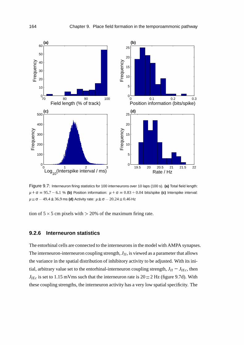
164 Chapter 9. Place field formation in the temporoammonic pathway
70 80 90 1000
10
20
30
40
50
60
Field length (% of track)
Fre
quen
cy
(a)
0 0.1 0.2 0.30
5
10
15
20
25
Position information (bits/spike)
Fre
quen
cy
(b)
0 1 2 30
100
200
300
400
500
Log10
(Interspike interval / ms)
Fre
quen
cy
(c)
19.5 20 20.5 21 21.5 220
5
10
15
20
25
Rate / Hz
Fre
quen
cy
(d)
Figure 9.7: Interneuron firing statistics for 100 interneurons over 10 laps (100 s). (a) Total field length:
µ � σ � 95 � 7 � 6 � 1 % (b) Position information: µ � σ � 0 � 83 � 0 � 04 bits/spike (c) Interspike interval:
µ � σ � 49 � 4 � 36 � 9 ms (d) Activity rate: µ � σ � 20 � 24 � 0 � 46 Hz
tion of 5 � 5 cm pixels with � 20% of the maximum firing rate.
9.2.6 Interneuron statistics
The entorhinal cells are connected to the interneurons in the model with AMPA synapses.
The interneuron-interneuron coupling strength, JII, is viewed as a parameter that allows
the variance in the spatial distribution of inhibitory activity to be adjusted. With its ini-
tial, arbitrary value set to the entorhinal-interneuron coupling strength, JII � JIEc, then
JIEc is set to 1.15 mVms such that the interneuron rate is 20�
2 Hz (figure 9.7d). With
these coupling strengths, the interneuron activity has a very low spatial specificity. The
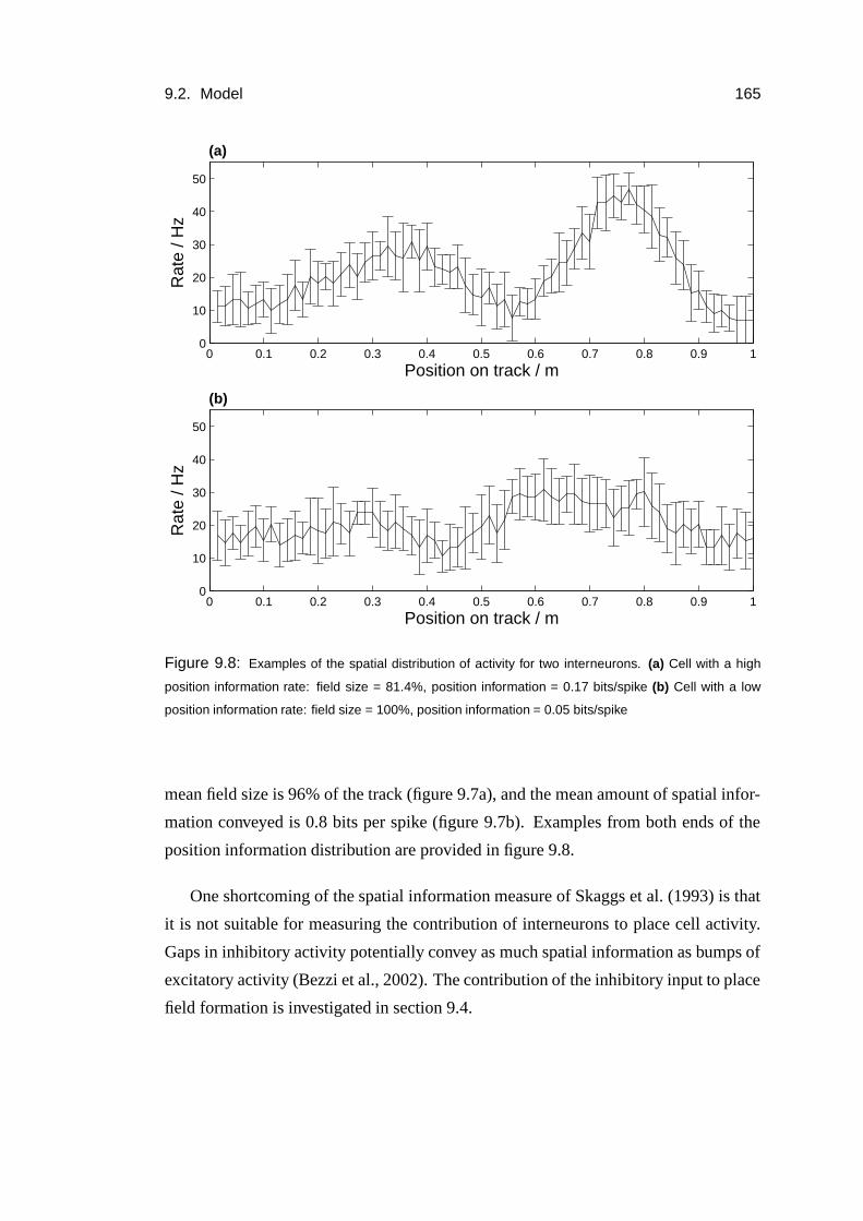
9.2. Model 165
0 0.1 0.2 0.3 0.4 0.5 0.6 0.7 0.8 0.9 10
10
20
30
40
50
Position on track / m
Rat
e / H
z
(b)
0 0.1 0.2 0.3 0.4 0.5 0.6 0.7 0.8 0.9 10
10
20
30
40
50
Position on track / m
Rat
e / H
z
(a)
Figure 9.8: Examples of the spatial distribution of activity for two interneurons. (a) Cell with a high
position information rate: field size = 81.4%, position information = 0.17 bits/spike (b) Cell with a low
position information rate: field size = 100%, position information = 0.05 bits/spike
mean field size is 96% of the track (figure 9.7a), and the mean amount of spatial infor-
mation conveyed is 0.8 bits per spike (figure 9.7b). Examples from both ends of the
position information distribution are provided in figure 9.8.
One shortcoming of the spatial information measure of Skaggs et al. (1993) is that
it is not suitable for measuring the contribution of interneurons to place cell activity.
Gaps in inhibitory activity potentially convey as much spatial information as bumps of
excitatory activity (Bezzi et al., 2002). The contribution of the inhibitory input to place
field formation is investigated in section 9.4.
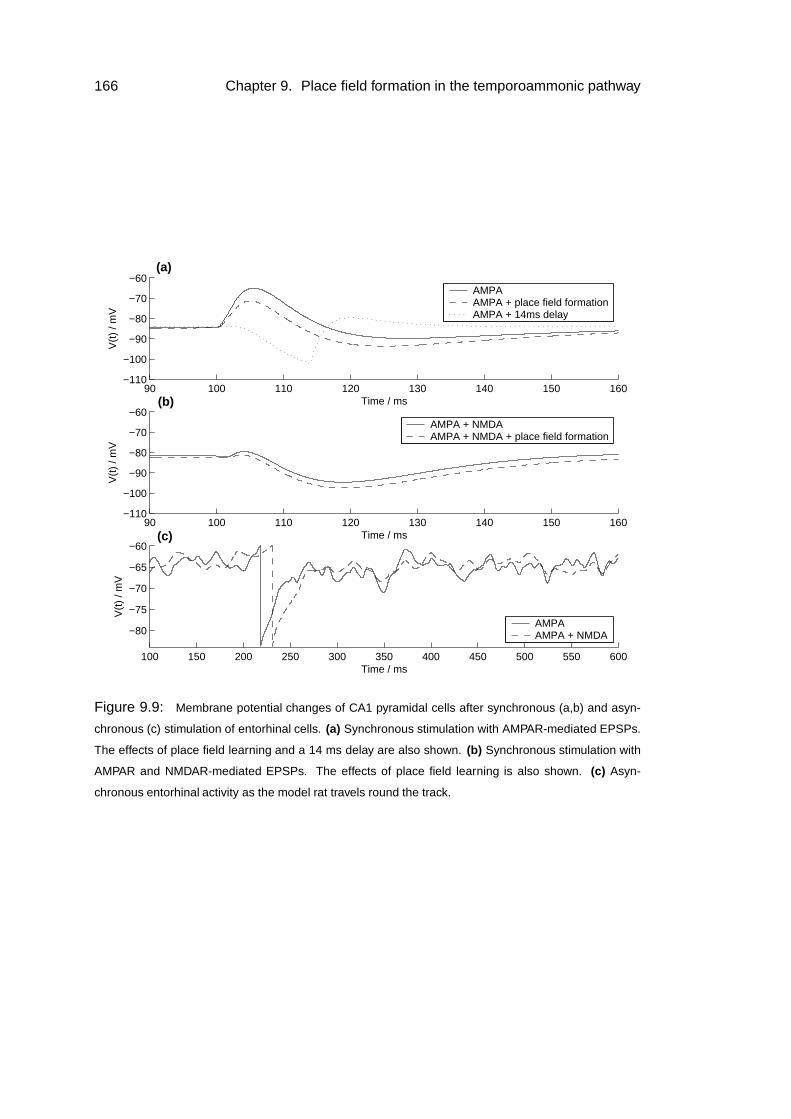
166 Chapter 9. Place field formation in the temporoammonic pathway
90 100 110 120 130 140 150 160−110
−100
−90
−80
−70
−60(a)
Time / ms
V(t
) / m
V
90 100 110 120 130 140 150 160−110
−100
−90
−80
−70
−60(b)
Time / ms
V(t
) / m
V
100 150 200 250 300 350 400 450 500 550 600
−80
−75
−70
−65
−60(c)
Time / ms
V(t
) / m
V
AMPAAMPA + place field formationAMPA + 14ms delay
AMPA + NMDAAMPA + NMDA + place field formation
AMPAAMPA + NMDA
Figure 9.9: Membrane potential changes of CA1 pyramidal cells after synchronous (a,b) and asyn-
chronous (c) stimulation of entorhinal cells. (a) Synchronous stimulation with AMPAR-mediated EPSPs.
The effects of place field learning and a 14 ms delay are also shown. (b) Synchronous stimulation with
AMPAR and NMDAR-mediated EPSPs. The effects of place field learning is also shown. (c) Asyn-
chronous entorhinal activity as the model rat travels round the track.
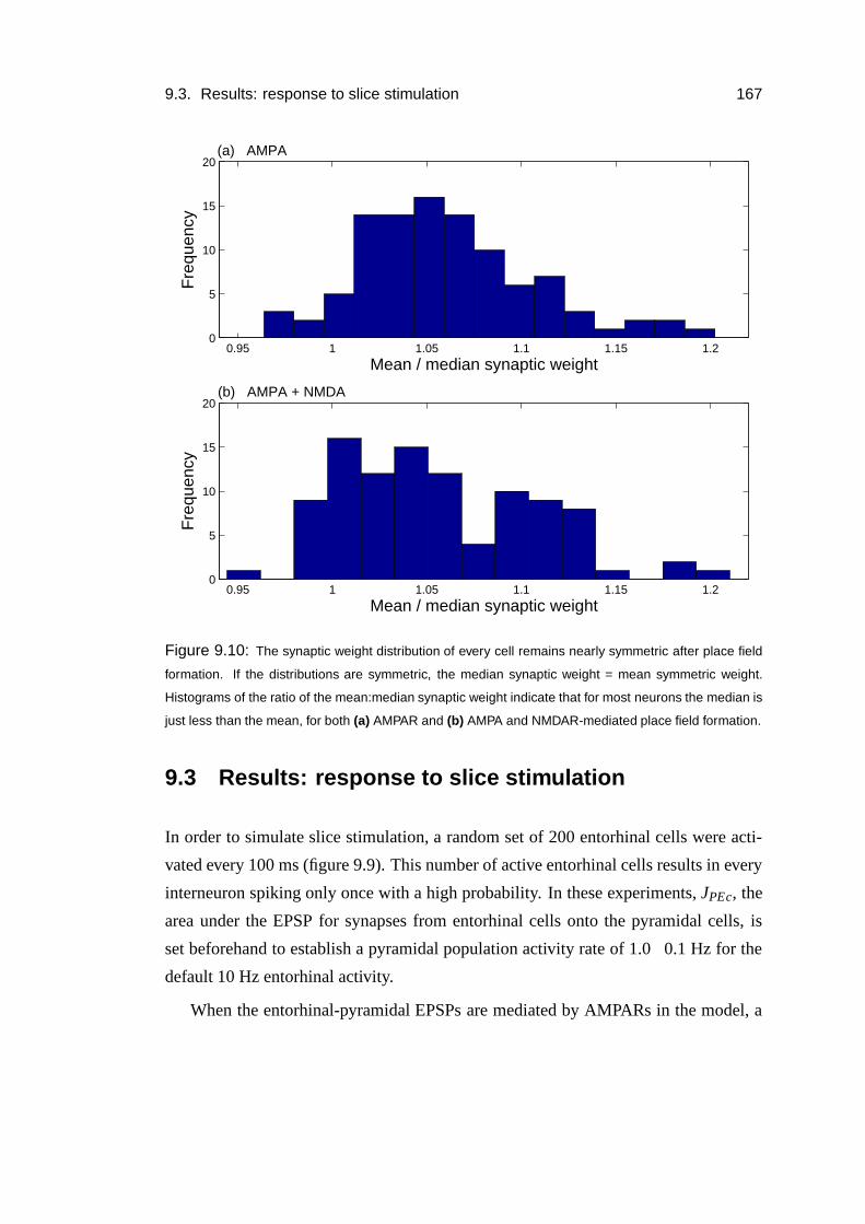
9.3. Results: response to slice stimulation 167
0.95 1 1.05 1.1 1.15 1.20
5
10
15
20
Mean / median synaptic weight
Fre
quen
cy
(a) AMPA
0.95 1 1.05 1.1 1.15 1.20
5
10
15
20
Mean / median synaptic weight
Fre
quen
cy
(b) AMPA + NMDA
Figure 9.10: The synaptic weight distribution of every cell remains nearly symmetric after place field
formation. If the distributions are symmetric, the median synaptic weight = mean symmetric weight.
Histograms of the ratio of the mean:median synaptic weight indicate that for most neurons the median is
just less than the mean, for both (a) AMPAR and (b) AMPA and NMDAR-mediated place field formation.
9.3 Results: response to slice stimulation
In order to simulate slice stimulation, a random set of 200 entorhinal cells were acti-
vated every 100 ms (figure 9.9). This number of active entorhinal cells results in every
interneuron spiking only once with a high probability. In these experiments, JPEc, the
area under the EPSP for synapses from entorhinal cells onto the pyramidal cells, is
set beforehand to establish a pyramidal population activity rate of 1.0�
0.1 Hz for the
default 10 Hz entorhinal activity.
When the entorhinal-pyramidal EPSPs are mediated by AMPARs in the model, a
168 Chapter 9. Place field formation in the temporoammonic pathway
clear excitatory response is observed, followed by a longer hyperpolarizing response
(figure 9.9a). This requires JPEc = 0.51 mVms to set the rate to 1 � 0�
0 � 1 Hz over
the first second. The excitatory response persists even when an unrealistically large
transmission delay of 14 ms is included, such that the EPSPs peak at the trough of the
inhibitory response, requiring JPEc = 2.0 mVms (figure 9.9a).
The response is biased in that the synaptic weights have initial random and similar
values in the model. After 10 laps of the track, the synaptic weights have functional
significance as place fields have successfully formed (section 9.4). Even so, the synap-
tic distribution is nearly symmetric, indicating that a large proportion of synapses are
responsible for the cells activity (figure 9.10a). The slice stimulus response is indeed
lower, but it still has a large depolarising phase (figure 9.9a). The low position infor-
mation conveyed by every superficial EC neuron means that it is highly unlikely that a
small subset of input weights will govern a cell’s activity. Therefore it is unlikely that
the lack of an excitatory response is due to the random selection of entorhinal activity
rather than a pattern of natural stimuli, as suggested by Buzsaki et al. (1995).
As discussed in section 3.2, it has often been assumed that temporoammonic synapses
lack a significant NMDA component (e.g. Soltesz, 1995). Otmakhova et al. (2002) re-
ported that the area under NMDAR-mediated EPSPs at temporoammonic synapses
is roughly three times that of AMPAR-mediated EPSPs (figure 3.3). Let us define
JPEcNMDA the area under the NMDAR-mediated PSP, and JPEcAMPA, the area under the
AMPAR-mediated EPSP, so that JPEcNMDA � 3 � JPEcAMPA.
When this NMDAR-mediated component is included in the EPSP, and an uniform
delay of 2 ms is inserted in the entorhinal-pyramidal transmission, setting JPEc = 0.14
mVms maintains the pyramidal cell population rate at 1 � 0�
0 � 1 Hz. Thus the total
area under the unit PSPs is only slightly larger at 0.56 mVms. The PSP response now
consists of a small depolarising phase, followed by a large hyperpolarisation. A small,
extended depolarising tail of the NMDA EPSP is just discernible (figure 9.9b). Once
the place fields have been learnt, the synaptic distribution is also nearly symmetric (fig-
ure 9.10b). Again, random stimulation now results in a more hyperpolarised response,
and the NMDA depolarising tail is no longer visible.
The effect of including the NMDAR-mediated component in the EPSP on the mem-
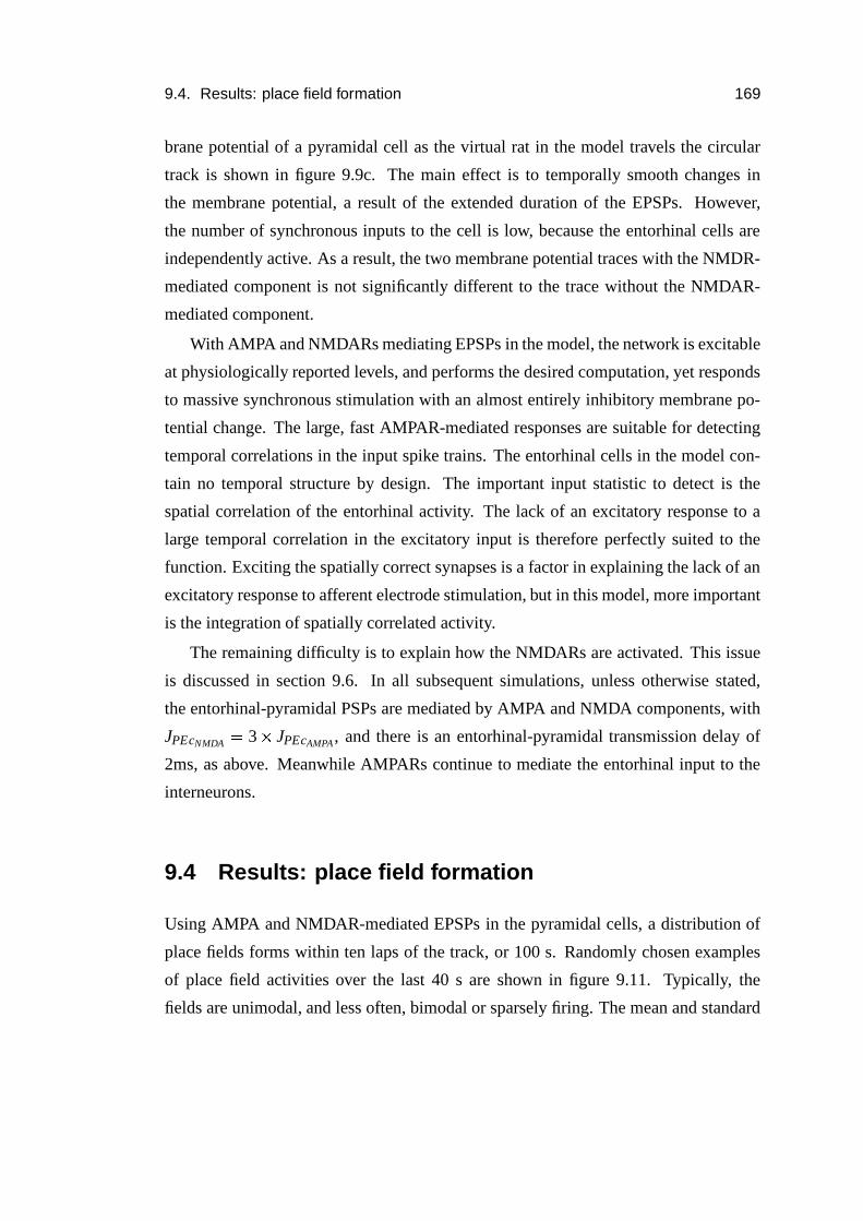
9.4. Results: place field formation 169
brane potential of a pyramidal cell as the virtual rat in the model travels the circular
track is shown in figure 9.9c. The main effect is to temporally smooth changes in
the membrane potential, a result of the extended duration of the EPSPs. However,
the number of synchronous inputs to the cell is low, because the entorhinal cells are
independently active. As a result, the two membrane potential traces with the NMDR-
mediated component is not significantly different to the trace without the NMDAR-
mediated component.
With AMPA and NMDARs mediating EPSPs in the model, the network is excitable
at physiologically reported levels, and performs the desired computation, yet responds
to massive synchronous stimulation with an almost entirely inhibitory membrane po-
tential change. The large, fast AMPAR-mediated responses are suitable for detecting
temporal correlations in the input spike trains. The entorhinal cells in the model con-
tain no temporal structure by design. The important input statistic to detect is the
spatial correlation of the entorhinal activity. The lack of an excitatory response to a
large temporal correlation in the excitatory input is therefore perfectly suited to the
function. Exciting the spatially correct synapses is a factor in explaining the lack of an
excitatory response to afferent electrode stimulation, but in this model, more important
is the integration of spatially correlated activity.
The remaining difficulty is to explain how the NMDARs are activated. This issue
is discussed in section 9.6. In all subsequent simulations, unless otherwise stated,
the entorhinal-pyramidal PSPs are mediated by AMPA and NMDA components, with
JPEcNMDA � 3 � JPEcAMPA, and there is an entorhinal-pyramidal transmission delay of
2ms, as above. Meanwhile AMPARs continue to mediate the entorhinal input to the
interneurons.
9.4 Results: place field formation
Using AMPA and NMDAR-mediated EPSPs in the pyramidal cells, a distribution of
place fields forms within ten laps of the track, or 100 s. Randomly chosen examples
of place field activities over the last 40 s are shown in figure 9.11. Typically, the
fields are unimodal, and less often, bimodal or sparsely firing. The mean and standard
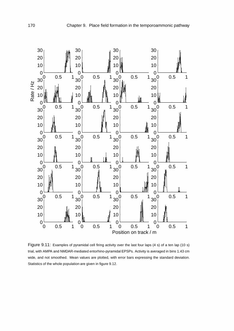
170 Chapter 9. Place field formation in the temporoammonic pathway
0 0.5 10
10
20
30
0 0.5 10
10
20
30
0 0.5 10
10
20
30
0 0.5 10
10
20
30
0 0.5 10
10
20
30
Rat
e / H
z
0 0.5 10
10
20
30
0 0.5 10
10
20
30
0 0.5 10
10
20
30
0 0.5 10
10
20
30
0 0.5 10
10
20
30
0 0.5 10
10
20
30
0 0.5 10
10
20
30
0 0.5 10
10
20
30
0 0.5 10
10
20
30
0 0.5 10
10
20
30
0 0.5 10
10
20
30
0 0.5 10
10
20
30
0 0.5 10
10
20
30
0 0.5 10
10
20
30
0 0.5 10
10
20
30
0 0.5 10
10
20
30
0 0.5 10
10
20
30
0 0.5 10
10
20
30
Position on track / m0 0.5 1
0
10
20
30
Figure 9.11: Examples of pyramidal cell firing activity over the last four laps (4 s) of a ten lap (10 s)
trial, with AMPA and NMDAR-mediated entorhino-pyramidal EPSPs. Activity is averaged in bins 1.43 cm
wide, and not smoothed. Mean values are plotted, with error bars expressing the standard deviation.
Statistics of the whole population are given in figure 9.12.
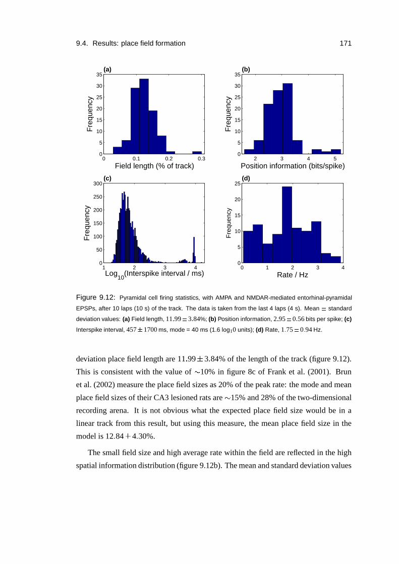
9.4. Results: place field formation 171
0 0.1 0.2 0.30
5
10
15
20
25
30
35
Field length (% of track)
Fre
quen
cy
(a)
2 3 4 50
5
10
15
20
25
30
35(b)
Position information (bits/spike)
Fre
quen
cy
1 2 3 40
50
100
150
200
250
300
Log10
(Interspike interval / ms)
Fre
quen
cy
(c)
0 1 2 3 40
5
10
15
20
25
Rate / Hz
(d)
Fre
quen
cy
Figure 9.12: Pyramidal cell firing statistics, with AMPA and NMDAR-mediated entorhinal-pyramidal
EPSPs, after 10 laps (10 s) of the track. The data is taken from the last 4 laps (4 s). Mean � standard
deviation values: (a) Field length, 11 � 99 � 3 � 84%; (b) Position information, 2 � 95 � 0 � 56 bits per spike; (c)
Interspike interval, 457 � 1700 ms, mode = 40 ms (1.6 log10 units); (d) Rate, 1 � 75 � 0 � 94 Hz.
deviation place field length are 11 � 99�
3 � 84% of the length of the track (figure 9.12).
This is consistent with the value of � 10% in figure 8c of Frank et al. (2001). Brun
et al. (2002) measure the place field sizes as 20% of the peak rate: the mode and mean
place field sizes of their CA3 lesioned rats are � 15% and 28% of the two-dimensional
recording arena. It is not obvious what the expected place field size would be in a
linear track from this result, but using this measure, the mean place field size in the
model is 12 � 84�
4 � 30%.
The small field size and high average rate within the field are reflected in the high
spatial information distribution (figure 9.12b). The mean and standard deviation values
172 Chapter 9. Place field formation in the temporoammonic pathway
0 0.5 1 1.5 2 2.5 3 3.5 41.5
2
2.5
3
3.5
4
4.5
5
5.5
Rate / Hz
Pos
ition
info
rmat
ion
(bits
/spi
ke)
AMPAAMPA + NMDA
Figure 9.13: The position information as a function of the rate, over the last 4 laps (40 s) of 10 laps
around the track, when either AMPA and NMDARs, or AMPARs alone mediate the entorhino-pyramidal
EPSPs. Correlation coefficients: AMPA and NMDA, -0.67, AMPA, -0.70.
are 2 � 95�
0 � 56 bits per spike. The distribution is somewhat higher and narrower than
the 2 � 34�
1 � 25 bits per spike reported by Frank et al. (2000). Because the place field
sizes are slightly larger, this implies that the firing rate within the place field is greater
in proportion to the average rate in the model than in Frank et al. (2000)’s data.
Brun et al. (2002) quantify the spatial information of CA1 pyramidal cell activity,
using the sparseness measure introduced by (Treves and Rolls, 1991). Over K spatial
bins, the sparseness of a cell is defined as
� ∑k rk � K � 2∑k r2
k � K(9.9)
where rk is the rate of the cell in the spatial bin k, and r2k is the square of the rate

9.4. Results: place field formation 173
0 10 20 30 40 50 60 70 80 90 1000
0.1
0.2
0.3
0.4
0.5
0.6
0.7
0.8
0.9
1
Position of cell in array
Pea
k ra
te lo
catio
n / m
Figure 9.14: Locations of the peak firing rate calculated from the last 4 laps, as a function of position
in the array. The correlation coefficient of position on the track and in the array is -0.09.
in that bin.
Brun et al. (2002) measured the median sparseness of CA1 pyramidal cells as 0.46
for CA3 lesioned rats, and 0.30 for the control rats. The mean and standard deviation
sparseness for the CA1 pyramidal cells in the model is 0 � 10�
0 � 04.
Both of the measures of spatial information are affected by the length of the time
bin. The interspike interval distribution is highly skewed (figure 9.12c). The mode is
40 ms, or 1.6 in log10 units, while the mean and standard deviation are 457�
1700
ms. There is a second peak at between 4000-4500ms, (3.60-3.65 in log10 units). This
corresponds to events in the secondary peaks. If the locations of the secondary peaks
are randomly located, the interspike interval distribution will be widely distributed with
a maximum, averaging across all cells, on the opposite side of the ring to the primary
peak. The mean place field size is 10 cm, so this is a distance of 45 cm away, or 4500
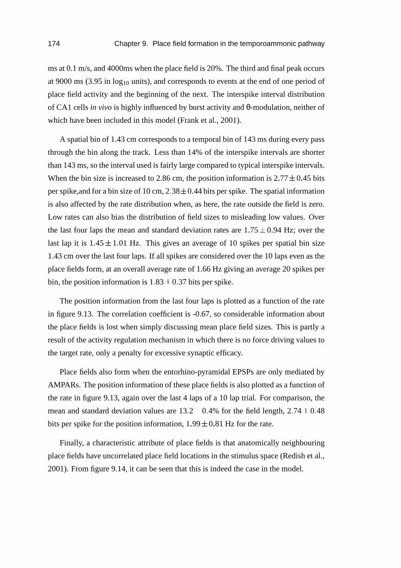
174 Chapter 9. Place field formation in the temporoammonic pathway
ms at 0.1 m/s, and 4000ms when the place field is 20%. The third and final peak occurs
at 9000 ms (3.95 in log10 units), and corresponds to events at the end of one period of
place field activity and the beginning of the next. The interspike interval distribution
of CA1 cells in vivo is highly influenced by burst activity and θ-modulation, neither of
which have been included in this model (Frank et al., 2001).
A spatial bin of 1.43 cm corresponds to a temporal bin of 143 ms during every pass
through the bin along the track. Less than 14% of the interspike intervals are shorter
than 143 ms, so the interval used is fairly large compared to typical interspike intervals.
When the bin size is increased to 2.86 cm, the position information is 2 � 77�
0 � 45 bits
per spike,and for a bin size of 10 cm, 2 � 38�
0 � 44 bits per spike. The spatial information
is also affected by the rate distribution when, as here, the rate outside the field is zero.
Low rates can also bias the distribution of field sizes to misleading low values. Over
the last four laps the mean and standard deviation rates are 1 � 75�
0 � 94 Hz; over the
last lap it is 1 � 45�
1 � 01 Hz. This gives an average of 10 spikes per spatial bin size
1.43 cm over the last four laps. If all spikes are considered over the 10 laps even as the
place fields form, at an overall average rate of 1.66 Hz giving an average 20 spikes per
bin, the position information is 1 � 83�
0 � 37 bits per spike.
The position information from the last four laps is plotted as a function of the rate
in figure 9.13. The correlation coefficient is -0.67, so considerable information about
the place fields is lost when simply discussing mean place field sizes. This is partly a
result of the activity regulation mechanism in which there is no force driving values to
the target rate, only a penalty for excessive synaptic efficacy.
Place fields also form when the entorhino-pyramidal EPSPs are only mediated by
AMPARs. The position information of these place fields is also plotted as a function of
the rate in figure 9.13, again over the last 4 laps of a 10 lap trial. For comparison, the
mean and standard deviation values are 13 � 2�
0 � 4% for the field length, 2 � 74�
0 � 48
bits per spike for the position information, 1 � 99�
0 � 81 Hz for the rate.
Finally, a characteristic attribute of place fields is that anatomically neighbouring
place fields have uncorrelated place field locations in the stimulus space (Redish et al.,
2001). From figure 9.14, it can be seen that this is indeed the case in the model.
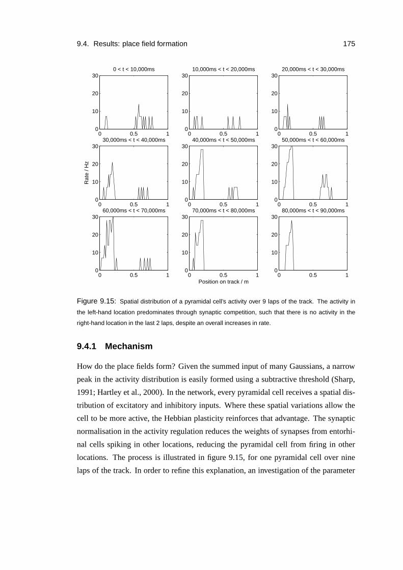
9.4. Results: place field formation 175
0 0.5 10
10
20
300 < t < 10,000ms
0 0.5 10
10
20
3010,000ms < t < 20,000ms
0 0.5 10
10
20
3020,000ms < t < 30,000ms
0 0.5 10
10
20
30
Rat
e / H
z
30,000ms < t < 40,000ms
0 0.5 10
10
20
3040,000ms < t < 50,000ms
0 0.5 10
10
20
3050,000ms < t < 60,000ms
0 0.5 10
10
20
3060,000ms < t < 70,000ms
0 0.5 10
10
20
30
Position on track / m
70,000ms < t < 80,000ms
0 0.5 10
10
20
3080,000ms < t < 90,000ms
Figure 9.15: Spatial distribution of a pyramidal cell’s activity over 9 laps of the track. The activity in
the left-hand location predominates through synaptic competition, such that there is no activity in the
right-hand location in the last 2 laps, despite an overall increases in rate.
9.4.1 Mechanism
How do the place fields form? Given the summed input of many Gaussians, a narrow
peak in the activity distribution is easily formed using a subtractive threshold (Sharp,
1991; Hartley et al., 2000). In the network, every pyramidal cell receives a spatial dis-
tribution of excitatory and inhibitory inputs. Where these spatial variations allow the
cell to be more active, the Hebbian plasticity reinforces that advantage. The synaptic
normalisation in the activity regulation reduces the weights of synapses from entorhi-
nal cells spiking in other locations, reducing the pyramidal cell from firing in other
locations. The process is illustrated in figure 9.15, for one pyramidal cell over nine
laps of the track. In order to refine this explanation, an investigation of the parameter
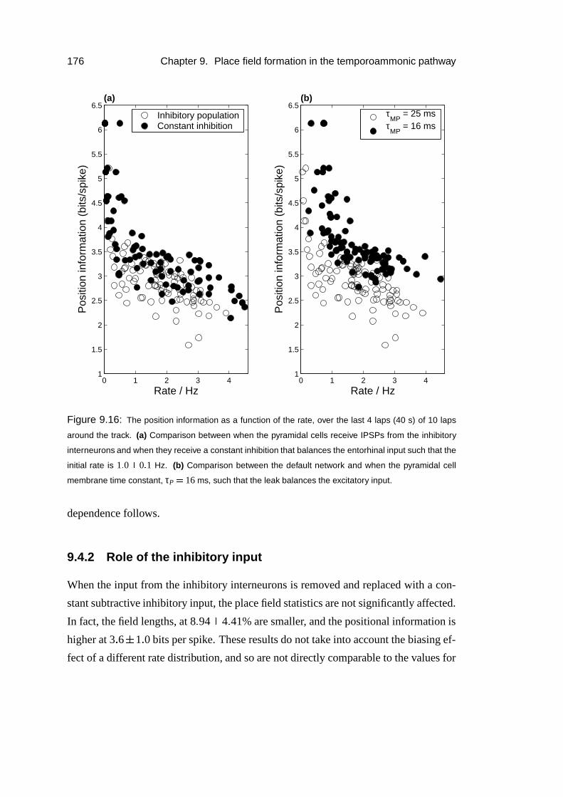
176 Chapter 9. Place field formation in the temporoammonic pathway
0 1 2 3 41
1.5
2
2.5
3
3.5
4
4.5
5
5.5
6
6.5(a)
Rate / Hz
Pos
ition
info
rmat
ion
(bits
/spi
ke)
0 1 2 3 41
1.5
2
2.5
3
3.5
4
4.5
5
5.5
6
6.5
Pos
ition
info
rmat
ion
(bits
/spi
ke)
Rate / Hz
(b)
Inhibitory populationConstant inhibition
τMP
= 25 msτ
MP = 16 ms
Figure 9.16: The position information as a function of the rate, over the last 4 laps (40 s) of 10 laps
around the track. (a) Comparison between when the pyramidal cells receive IPSPs from the inhibitory
interneurons and when they receive a constant inhibition that balances the entorhinal input such that the
initial rate is 1 � 0 � 0 � 1 Hz. (b) Comparison between the default network and when the pyramidal cell
membrane time constant, τP � 16 ms, such that the leak balances the excitatory input.
dependence follows.
9.4.2 Role of the inhibitory input
When the input from the inhibitory interneurons is removed and replaced with a con-
stant subtractive inhibitory input, the place field statistics are not significantly affected.
In fact, the field lengths, at 8 � 94�
4 � 41% are smaller, and the positional information is
higher at 3 � 6�
1 � 0 bits per spike. These results do not take into account the biasing ef-
fect of a different rate distribution, and so are not directly comparable to the values for
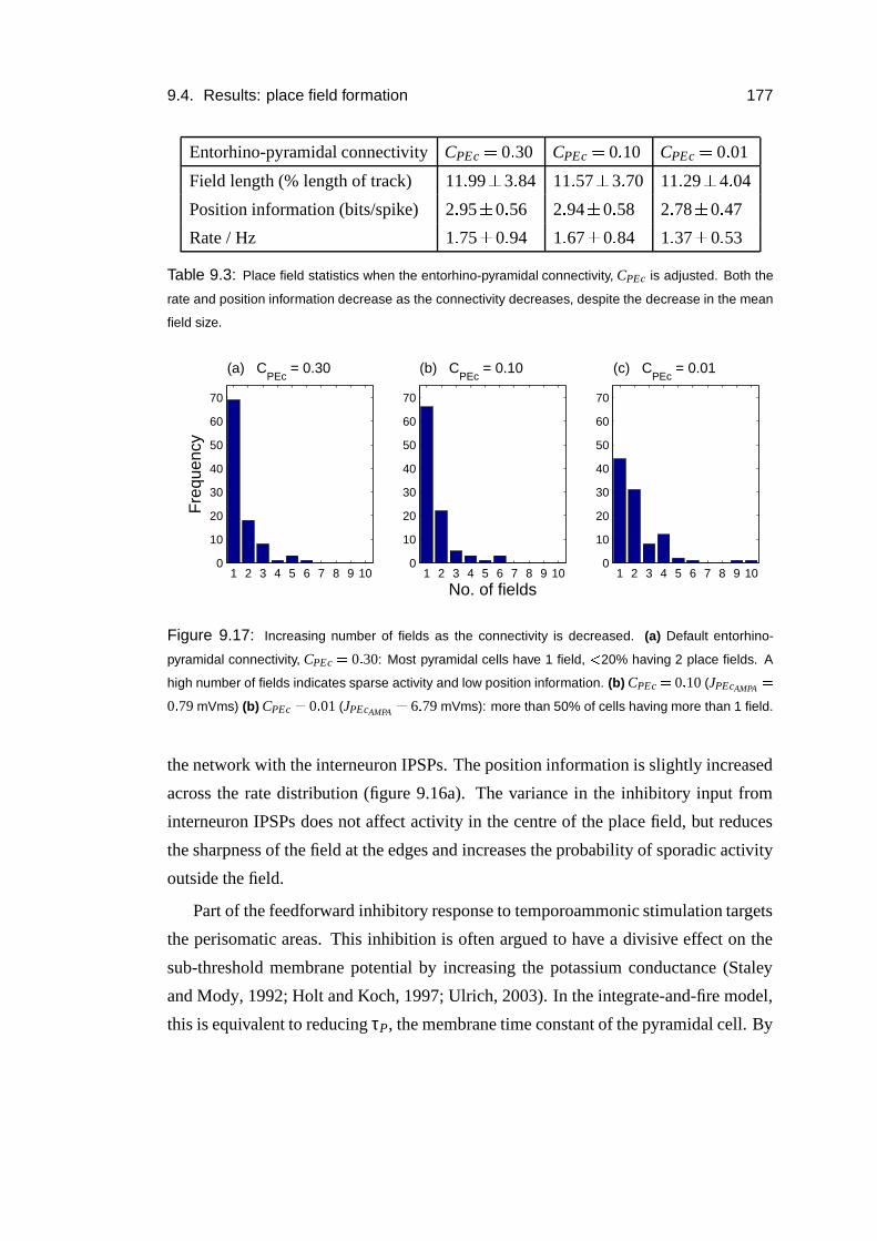
9.4. Results: place field formation 177
Entorhino-pyramidal connectivity CPEc � 0 � 30 CPEc � 0 � 10 CPEc � 0 � 01
Field length (% length of track) 11 � 99�
3 � 84 11 � 57�
3 � 70 11 � 29�
4 � 04
Position information (bits/spike) 2 � 95�
0 � 56 2 � 94�
0 � 58 2 � 78�
0 � 47
Rate / Hz 1 � 75�
0 � 94 1 � 67�
0 � 84 1 � 37�
0 � 53
Table 9.3: Place field statistics when the entorhino-pyramidal connectivity, CPEc is adjusted. Both the
rate and position information decrease as the connectivity decreases, despite the decrease in the mean
field size.
1 2 3 4 5 6 7 8 9 100
10
20
30
40
50
60
70
Fre
quen
cy
(a) CPEc
= 0.30
1 2 3 4 5 6 7 8 9 100
10
20
30
40
50
60
70
No. of fields
(b) CPEc
= 0.10
1 2 3 4 5 6 7 8 9 100
10
20
30
40
50
60
70
(c) CPEc
= 0.01
Figure 9.17: Increasing number of fields as the connectivity is decreased. (a) Default entorhino-
pyramidal connectivity, CPEc � 0 � 30: Most pyramidal cells have 1 field, � 20% having 2 place fields. A
high number of fields indicates sparse activity and low position information. (b) CPEc � 0 � 10 (JPEcAMPA �
0 � 79 mVms) (b) CPEc � 0 � 01 (JPEcAMPA � 6 � 79 mVms): more than 50% of cells having more than 1 field.
the network with the interneuron IPSPs. The position information is slightly increased
across the rate distribution (figure 9.16a). The variance in the inhibitory input from
interneuron IPSPs does not affect activity in the centre of the place field, but reduces
the sharpness of the field at the edges and increases the probability of sporadic activity
outside the field.
Part of the feedforward inhibitory response to temporoammonic stimulation targets
the perisomatic areas. This inhibition is often argued to have a divisive effect on the
sub-threshold membrane potential by increasing the potassium conductance (Staley
and Mody, 1992; Holt and Koch, 1997; Ulrich, 2003). In the integrate-and-fire model,
this is equivalent to reducing τP, the membrane time constant of the pyramidal cell. By
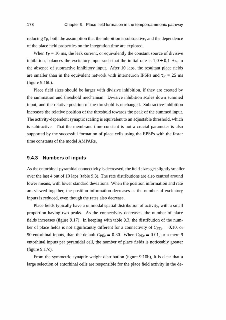
178 Chapter 9. Place field formation in the temporoammonic pathway
reducing τP, both the assumption that the inhibition is subtractive, and the dependence
of the place field properties on the integration time are explored.
When τP = 16 ms, the leak current, or equivalently the constant source of divisive
inhibition, balances the excitatory input such that the initial rate is 1 � 0�
0 � 1 Hz, in
the absence of subtractive inhibitory input. After 10 laps, the resultant place fields
are smaller than in the equivalent network with interneuron IPSPs and τP = 25 ms
(figure 9.16b).
Place field sizes should be larger with divisive inhibition, if they are created by
the summation and threshold mechanism. Divisive inhibition scales down summed
input, and the relative position of the threshold is unchanged. Subtractive inhibition
increases the relative position of the threshold towards the peak of the summed input.
The activity-dependent synaptic scaling is equivalent to an adjustable threshold, which
is subtractive. That the membrane time constant is not a crucial parameter is also
supported by the successful formation of place cells using the EPSPs with the faster
time constants of the model AMPARs.
9.4.3 Numbers of inputs
As the entorhinal-pyramidal connectivity is decreased, the field sizes get slightly smaller
over the last 4 out of 10 laps (table 9.3). The rate distributions are also centred around
lower means, with lower standard deviations. When the position information and rate
are viewed together, the position information decreases as the number of excitatory
inputs is reduced, even though the rates also decrease.
Place fields typically have a unimodal spatial distribution of activity, with a small
proportion having two peaks. As the connectivity decreases, the number of place
fields increases (figure 9.17). In keeping with table 9.3, the distribution of the num-
ber of place fields is not significantly different for a connectivity of CPEc � 0 � 10, or
90 entorhinal inputs, than the default CPEc � 0 � 30. When CPEc � 0 � 01, or a mere 9
entorhinal inputs per pyramidal cell, the number of place fields is noticeably greater
(figure 9.17c).
From the symmetric synaptic weight distribution (figure 9.10b), it is clear that a
large selection of entorhinal cells are responsible for the place field activity in the de-
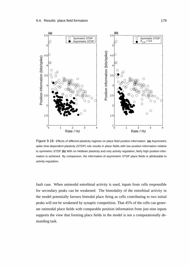
9.4. Results: place field formation 179
0 1 2 3 41
1.5
2
2.5
3
3.5
4
4.5
5
5.5
Rate / Hz
Pos
ition
info
rmat
ion
(bits
/spi
ke)
(a)
0 1 2 3 41
1.5
2
2.5
3
3.5
4
4.5
5
5.5
Pos
ition
info
rmat
ion
(bits
/spi
ke)
(b)
Rate / Hz
Symmetric STDPAsymmetric STDP
Symmetric STDPA
LTP = 0.0
Figure 9.18: Effects of different plasticity regimes on place field position information. (a) Asymmetric
spike time-dependent plasticity (STDP) rule results in place fields with low position information relative
to symmetric STDP. (b) With no Hebbian plasticity and only activity regulation, fairly high position infor-
mation is achieved. By comparison, the information of asymmetric STDP place fields is attributable to
activity regulation.
fault case. When unimodal entorhinal activity is used, inputs from cells responsible
for secondary peaks can be weakened. The bimodality of the entorhinal activity in
the model potentially favours bimodal place firing as cells contributing to two initial
peaks will not be weakened by synaptic competition. That 45% of the cells can gener-
ate unimodal place fields with comparable position information from just nine inputs
supports the view that forming place fields in the model is not a computationally de-
manding task.
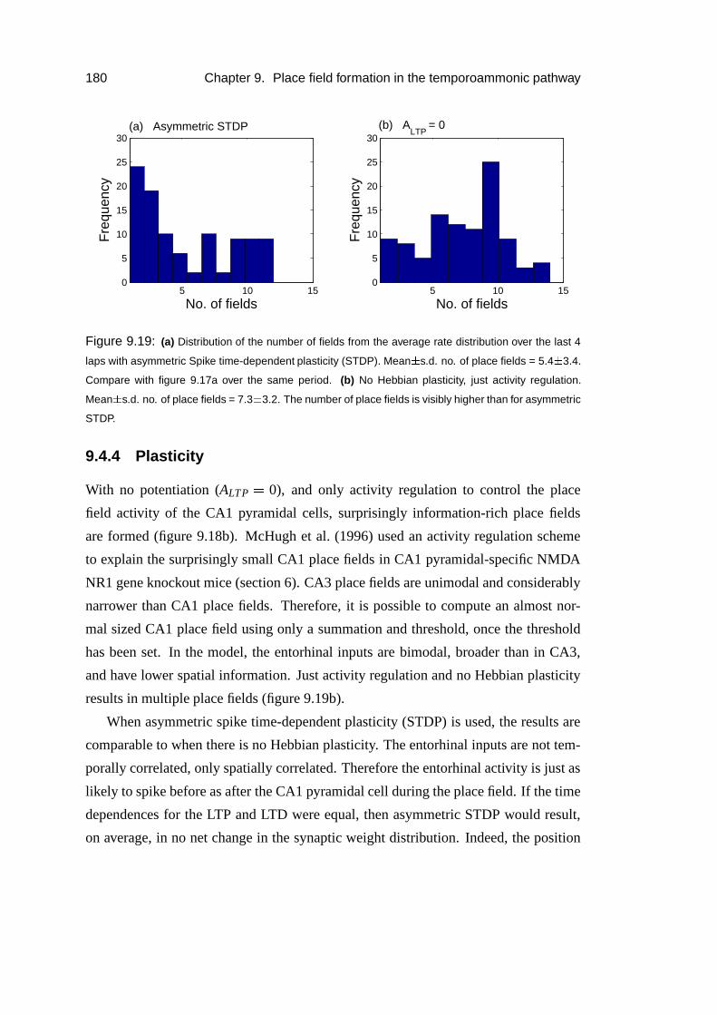
180 Chapter 9. Place field formation in the temporoammonic pathway
5 10 150
5
10
15
20
25
30
No. of fields
Fre
quen
cy
(a) Asymmetric STDP
5 10 150
5
10
15
20
25
30
Fre
quen
cy
No. of fields
(b) ALTP
= 0
Figure 9.19: (a) Distribution of the number of fields from the average rate distribution over the last 4
laps with asymmetric Spike time-dependent plasticity (STDP). Mean � s.d. no. of place fields = 5.4 � 3.4.
Compare with figure 9.17a over the same period. (b) No Hebbian plasticity, just activity regulation.
Mean � s.d. no. of place fields = 7.3 � 3.2. The number of place fields is visibly higher than for asymmetric
STDP.
9.4.4 Plasticity
With no potentiation (ALTP � 0), and only activity regulation to control the place
field activity of the CA1 pyramidal cells, surprisingly information-rich place fields
are formed (figure 9.18b). McHugh et al. (1996) used an activity regulation scheme
to explain the surprisingly small CA1 place fields in CA1 pyramidal-specific NMDA
NR1 gene knockout mice (section 6). CA3 place fields are unimodal and considerably
narrower than CA1 place fields. Therefore, it is possible to compute an almost nor-
mal sized CA1 place field using only a summation and threshold, once the threshold
has been set. In the model, the entorhinal inputs are bimodal, broader than in CA3,
and have lower spatial information. Just activity regulation and no Hebbian plasticity
results in multiple place fields (figure 9.19b).
When asymmetric spike time-dependent plasticity (STDP) is used, the results are
comparable to when there is no Hebbian plasticity. The entorhinal inputs are not tem-
porally correlated, only spatially correlated. Therefore the entorhinal activity is just as
likely to spike before as after the CA1 pyramidal cell during the place field. If the time
dependences for the LTP and LTD were equal, then asymmetric STDP would result,
on average, in no net change in the synaptic weight distribution. Indeed, the position
9.5. Place field formation in similar environments 181
information distribution (figure 9.18a) is comparable to the case with no plasticity (fig-
ure 9.18b). There can be a small net gain in synaptic weight at a place field because
τLTD � τLTP. This is reflected in the distribution in the number of fields (figure 9.19a),
which is biased towards a lower number of fields compared to the no plasticity case
(figure 9.19b).
9.5 Place field formation in similar environments
What is the function of the temporoammonic pathway? So far, three positions have
been developed:
� The rate of plasticity in the temporoammonic pathway must be lower than in the
Schaffer collaterals, due to the lower capacity of the temporoammonic pathway
(section 7.4.3).
� It is computationally advantageous for the Schaffer collaterals to form the initial
pattern of activity in CA1 during place field formation, in terms of increased
capacity and simpler thresholding implementation (section 8.7).
� Place field formation in the temporoammonic pathway is robust, and is supported
by low connectivities (section 9.4).
The long-term plasticity of place field locations of similar environments (Lever
et al., 2002, section 4.3.3) is an experimental finding that can potentially be explained
by the plasticity in the temporoammonic pathway.
The finding has an intuitive significance for behaviour. The hippocampus has a crit-
ical role in the memory of one-trial events (Nakazawa et al., 2003) and in establishing a
spatial map of an environment (O’Keefe and Nadel, 1978). When similar environments
are not initially perceived as being different, the representations of stored events will
be correlated through a shared representation of space. CA1 could allow the represen-
tations of the environments to become uncorrelated, as a function of experience, whilst
maintaining the stored record of events. This strategy would allow the hippocampus
to support both the rapid acquisition of memories of attended events, and to benefit
182 Chapter 9. Place field formation in the temporoammonic pathway
from experience in developing perceptions of distinct spatial contexts. In the case of a
spatial cue manipulation the perception of difference is sensory, and once noticed, the
environment could be treated as novel if integrated perceptions of localisation are first
formed in the hippocampus.
Lever et al. (2002) report three ways in which the place fields diverge:
� Changes in rate
� Discrete field relocalisation
� Smooth field relocalisation
The first two can be explained by competitive learning. For instance, a presynaptic
covariance rule will orthogonalise the correlated inputs by promoting different cells
to be active in response to different input patterns (Minai, 1997). For two neurons
both initially active to a pair of correlated inputs, one cell will come to represent one
pattern, and the other cell the other pattern. These changes can account for changes in
rate and new fields appearing, but what process supports the same cell being active in
increasingly different locations on the tracks? One candidate is lateral inhibition: the
initial CA3 input established CA1 place map is randomly rearranged to minimise the
lateral inhibition. However, if the place fields have been learnt by Hebbian learning
as in the previous sections, the synapses active in the same locations on each track
will be potentiated at a faster rate than the synapses which are not. This will promote
correlated activity despite the lateral inhibition.
The purpose of the experiments that follow is to explore the consequences of tem-
poroammonic plasticity for place fields formed by CA3 input. The dynamics of CA3
do not directly concern us, so CA3 input is modelled by the spatially consistent activa-
tion of the CA1 pyramidal neurons, in addition to the effects of entorhinal input. The
reduction in the strength of the Schaffer collateral input is modelled by the removal
of the CA3 input. This extreme implementation allows us to identify the effects of
temporoammonic plasticity alone.
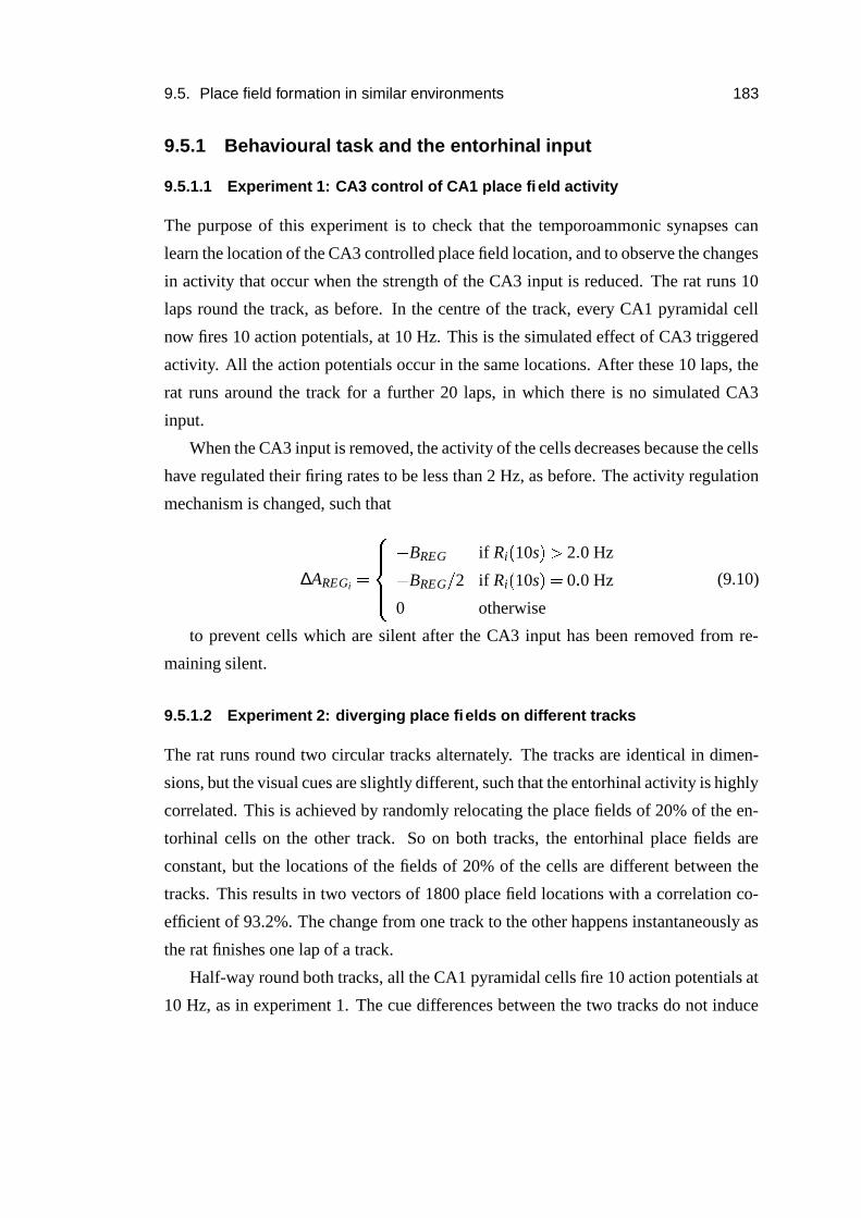
9.5. Place field formation in similar environments 183
9.5.1 Behavioural task and the entorhinal input
9.5.1.1 Experiment 1: CA3 control of CA1 place field activity
The purpose of this experiment is to check that the temporoammonic synapses can
learn the location of the CA3 controlled place field location, and to observe the changes
in activity that occur when the strength of the CA3 input is reduced. The rat runs 10
laps round the track, as before. In the centre of the track, every CA1 pyramidal cell
now fires 10 action potentials, at 10 Hz. This is the simulated effect of CA3 triggered
activity. All the action potentials occur in the same locations. After these 10 laps, the
rat runs around the track for a further 20 laps, in which there is no simulated CA3
input.
When the CA3 input is removed, the activity of the cells decreases because the cells
have regulated their firing rates to be less than 2 Hz, as before. The activity regulation
mechanism is changed, such that
∆AREGi ����� ���
� BREG if Ri � 10s � � 2 � 0 Hz�
BREG � 2 if Ri � 10s � � 0 � 0 Hz
0 otherwise
(9.10)
to prevent cells which are silent after the CA3 input has been removed from re-
maining silent.
9.5.1.2 Experiment 2: diverging place fields on different tracks
The rat runs round two circular tracks alternately. The tracks are identical in dimen-
sions, but the visual cues are slightly different, such that the entorhinal activity is highly
correlated. This is achieved by randomly relocating the place fields of 20% of the en-
torhinal cells on the other track. So on both tracks, the entorhinal place fields are
constant, but the locations of the fields of 20% of the cells are different between the
tracks. This results in two vectors of 1800 place field locations with a correlation co-
efficient of 93.2%. The change from one track to the other happens instantaneously as
the rat finishes one lap of a track.
Half-way round both tracks, all the CA1 pyramidal cells fire 10 action potentials at
10 Hz, as in experiment 1. The cue differences between the two tracks do not induce
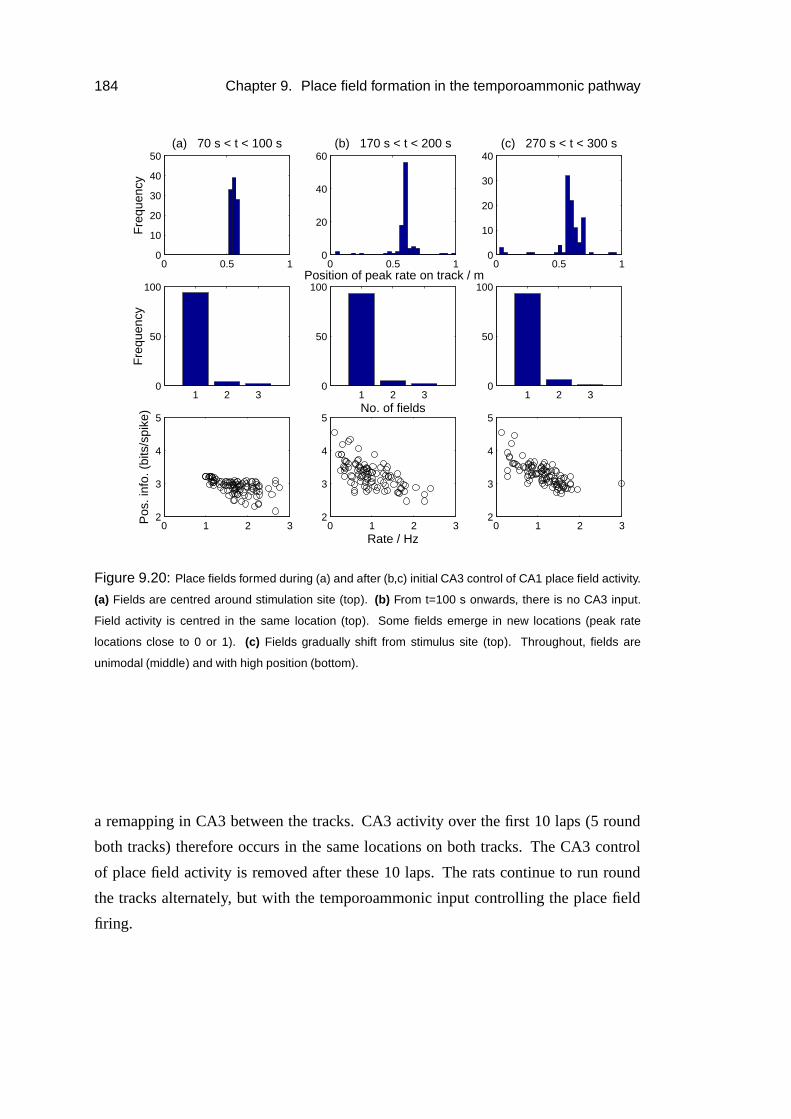
184 Chapter 9. Place field formation in the temporoammonic pathway
0 0.5 10
10
20
30
40(c) 270 s < t < 300 s
1 2 30
50
100
0 1 2 32
3
4
5
0 0.5 10
10
20
30
40
50(a) 70 s < t < 100 s
Fre
quen
cy
1 2 30
50
100
Fre
quen
cy
0 1 2 32
3
4
5
Pos
. inf
o. (
bits
/spi
ke)
0 0.5 10
20
40
60
Position of peak rate on track / m
(b) 170 s < t < 200 s
1 2 30
50
100
No. of fields
0 1 2 32
3
4
5
Rate / Hz
Figure 9.20: Place fields formed during (a) and after (b,c) initial CA3 control of CA1 place field activity.
(a) Fields are centred around stimulation site (top). (b) From t=100 s onwards, there is no CA3 input.
Field activity is centred in the same location (top). Some fields emerge in new locations (peak rate
locations close to 0 or 1). (c) Fields gradually shift from stimulus site (top). Throughout, fields are
unimodal (middle) and with high position (bottom).
a remapping in CA3 between the tracks. CA3 activity over the first 10 laps (5 round
both tracks) therefore occurs in the same locations on both tracks. The CA3 control
of place field activity is removed after these 10 laps. The rats continue to run round
the tracks alternately, but with the temporoammonic input controlling the place field
firing.
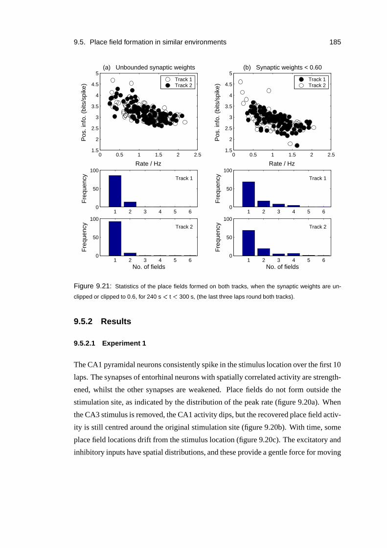
9.5. Place field formation in similar environments 185
1 2 3 4 5 60
50
100
Fre
quen
cy
1 2 3 4 5 60
50
100
No. of fields
Fre
quen
cy
1 2 3 4 5 60
50
100
No. of fields
Fre
quen
cy1 2 3 4 5 6
0
50
100
Fre
quen
cy
0 0.5 1 1.5 2 2.51.5
2
2.5
3
3.5
4
4.5
5
Rate / Hz
(b) Synaptic weights < 0.60
Pos
. inf
o. (
bits
/spi
ke)
0 0.5 1 1.5 2 2.51.5
2
2.5
3
3.5
4
4.5
5
Rate / Hz
Pos
. inf
o. (
bits
/spi
ke)
(a) Unbounded synaptic weights
Track 1Track 2
Track 1Track 2
Track 1
Track 2
Track 1
Track 2
Figure 9.21: Statistics of the place fields formed on both tracks, when the synaptic weights are un-
clipped or clipped to 0.6, for 240 s � t � 300 s, (the last three laps round both tracks).
9.5.2 Results
9.5.2.1 Experiment 1
The CA1 pyramidal neurons consistently spike in the stimulus location over the first 10
laps. The synapses of entorhinal neurons with spatially correlated activity are strength-
ened, whilst the other synapses are weakened. Place fields do not form outside the
stimulation site, as indicated by the distribution of the peak rate (figure 9.20a). When
the CA3 stimulus is removed, the CA1 activity dips, but the recovered place field activ-
ity is still centred around the original stimulation site (figure 9.20b). With time, some
place field locations drift from the stimulus location (figure 9.20c). The excitatory and
inhibitory inputs have spatial distributions, and these provide a gentle force for moving
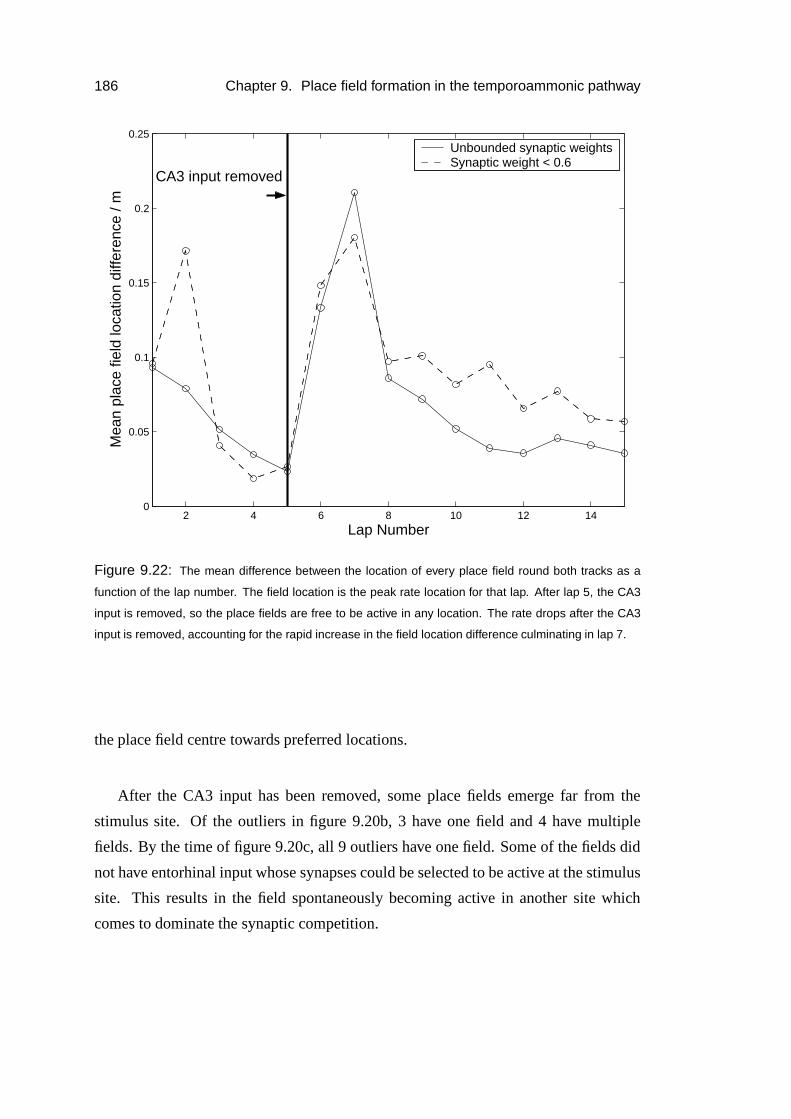
186 Chapter 9. Place field formation in the temporoammonic pathway
2 4 6 8 10 12 140
0.05
0.1
0.15
0.2
0.25
Lap Number
Mea
n pl
ace
field
loca
tion
diffe
renc
e / m
Unbounded synaptic weightsSynaptic weight < 0.6
CA3 input removed
Figure 9.22: The mean difference between the location of every place field round both tracks as a
function of the lap number. The field location is the peak rate location for that lap. After lap 5, the CA3
input is removed, so the place fields are free to be active in any location. The rate drops after the CA3
input is removed, accounting for the rapid increase in the field location difference culminating in lap 7.
the place field centre towards preferred locations.
After the CA3 input has been removed, some place fields emerge far from the
stimulus site. Of the outliers in figure 9.20b, 3 have one field and 4 have multiple
fields. By the time of figure 9.20c, all 9 outliers have one field. Some of the fields did
not have entorhinal input whose synapses could be selected to be active at the stimulus
site. This results in the field spontaneously becoming active in another site which
comes to dominate the synaptic competition.
9.5. Place field formation in similar environments 187
9.5.2.2 Experiment 2
As in experiment 1, the CA3 place field locations are learnt within the first 10 laps
of the track. Averaging over both tracks, the fields are not significantly different from
those learnt in experiment 1 over the same time range, despite the more variable spatial
correlations in the entorhinal activity. After the CA3 input has been removed, the place
field activity remains unimodal and high in position information (figure 9.21a). The
place fields tend to remain close to the CA3 input stimulation site for both tracks (data
not shown).
The evolution of the mean distance between every cell’s place fields on the two
tracks is shown in figure 9.22 ( ‘unbounded synaptic weights’ in the figure). The place
fields on the two tracks are initially separated by a mean distance of 9.3 cm. This
reflects the different preferred place field locations resulting from the different spatial
distributions of entorhinal input. The mean distance reduces to 2.3 cm by the fifth lap
as the CA3 controlled place locations over the first 100 s are learnt. The CA1 pyramidal
cell rate distribution drops after the CA3 input is removed, and activity regulation takes
a few laps to recover the rate distribution. By the tenth lap, the place fields have been
largely learnt again and the mean separation is 3.56 cm.
The majority of place fields are in similar locations on both tracks. Synapses that
are active in place fields on both tracks are potentiated faster than those only active on
one track. This has the effect of pulling the fields towards the same location on both
tracks. What mechanism can be used to maintain the place fields on both tracks, but
to move them apart? Because the same output cell is active to both sets of inputs, the
mechanism cannot be presynaptic. Ideally, the weights active in both locations would
be weakened, and the less frequently active synapses would be potentiated.
When the weights are clipped, so that they cannot exceed 0.6, the place fields form
by the fifth lap, as indicated by the average separation of 2.6 cm (figure 9.22). The
place fields after 30 laps (15 round both tracks) are further apart at 5.68 cm than with
unclipped Hebbian learning.
The upper limit on the synaptic weight prevents synapses active in the same loca-
tion on both tracks from dominating the place activity. This has the knock on effect of
increasing the potentiation of more infrequently active synapses. As established ear-
188 Chapter 9. Place field formation in the temporoammonic pathway
lier, narrow CA1 place fields can be maintained in the model by entorhinal cells with
a symmetric synaptic weight distribution. The larger set of entorhinal cells supporting
the place cell activity mean that the field is more likely to have a different preferred
location.
The clipped network also takes longer to learn the place fields in the absence of
CA3 input: the synapses active only on one track may be potentiated proportionally
more, but this occurs at a slower rate than for the synapses active on both tracks in the
unclipped network. This is reflected in the larger number of place fields and slightly
lower position information over the last 3 laps (figure 9.21b).
9.6 Discussion
The hyperpolarising somatic response to temporoammonic stimulation is consistent
with functional CA1 activity in the model when the polarising response occurs over a
long period of time relative to the inhibitory response. The model provides a demon-
stration of this point. It can be concluded that the hyperpolarizing response does not
imply that temporoammonic input cannot cause CA1 activity (Levy et al., 1995).
The explanation is consistent with the distal location of temporoammonic inputs to
CA1 pyramidal cells, and with the nature of the superficial entorhinal activity. Passive
propagation from the stratum lacunosum-moleculare to the soma will attenuate and
widen an EPSP. In the absence of active ion channels, the time of an input encoded in
a brief, high amplitude EPSP will become noisy. Dendritic spikes may minimise the
loss of this information, and could also signal coincident activity. There would appear
to be no advantage to detecting coincident entorhinal activity, given the low spatial
information and apparent lack of temporal correlation in superficial entorhinal activity.
In contrast, CA3 activity has significant temporal correlations, and many mechanisms
support the encoding of CA3 input spike times. The input spike times are encoded
by brief EPSPs, the synapses are located relatively proximal to the soma, and spike
time-dependent plasticity is observed (Nishiyama et al., 2000).
The contribution of NMDARs to EPSPs is difficult to predict because of their volt-
age dependence. Changes in the local membrane potential are sensitive to the local
9.6. Discussion 189
spatial arrangement. In the stratum radiatum, the localisation of Schaffer collateral
synapses on spines allows the effects of individual EPSPs on the local calcium con-
centration and membrane potential to be localised (Sabatini et al., 2002). In the stra-
tum lacunosum-moleculare, the density of spines drops dramatically, and the propor-
tion of asymmetric synapses contacting the dendritic shaft directly increases (Megıas
et al., 2001). In the absence of localising effects of dendritic morphology, the stra-
tum lacunosum-moleculare NMDARs of a particular cell will be activated by the mean
input rate of the cell.
In the model, the NMDAR-mediated component of the EPSPs was not modulated
by the membrane potential. If the stratum lacunosum-moleculare NMDARs of a cell
do respond as a population to the mean rate of the temporoammonic input, then this
is an acceptable first approximation. The model also assumes that LTP is expressed
as an equal increase in the voltage changes with time of the NMDA and AMPARs.
This is contrary to the proposed implementation of Marr’s self-organisation algorithm
discussed in section 8.7.2. The NMDA component of Schaffer collateral synapses
should remain constant for the implementation of Marr’s algorithm to work. It is not
crucial to the model that NMDA receptors express LTP as place fields are learnt in the
model with AMPARs alone. NMDARs in the stratum lacunosum-moleculare exhibit
inward rectification, unlike those in the stratum radiatum (Otmakhova et al., 2002).
That the NMDARs in the two layers have different properties is consistent with them
having different functions.
Place fields are formed in the model by Hebbian learning strengthening local spatial
correlations of entorhinal input. The ease of the task is partly because the model did
not have to generate many place field properties. For instance, the place fields reported
by Brun et al. (2002) are directional. In the model, the directionality of CA1 place
fields would have to come from the directionality of the inputs. The previous studies
of entorhinal activity do not mention their directionality, so the model is falsifiable on
this issue.
Place field activity can be supported in the model by a large number of entorhinal
inputs. If temporoammonically driven place field activity is associated with a large
number of entorhinal cells, then place fields can be maintained by spatially correlated

190 Chapter 9. Place field formation in the temporoammonic pathway
changes in the input rate. Entorhinal neurons conveys little spatial information com-
pared to CA1 pyramidal cells, and their activity is temporally uncorrelated by cross-
correlograms. Place field activity will be more reliable if it is supported by a large
population of entorhinal cells rather than a select few.
In the model, clipped Hebbian learning was used to prevent synaptic competition
from associating the place field activity to a few entorhinal inputs. An alternative im-
plementation would be place fields learnt by LTD, with activity regulation normalising
synaptic weight changes, as before. Low frequency stimulation of temporoammonic
afferents in the entorhinal-CA1 slice results in LTD, which is recovered by a period of
high frequency stimulation (Dvorak-Carbone and Schuman, 1999a, see section 3.2).
The implications and the success of this implementation is one focus of current work.
When the CA1 pyramidal cells spike in a given location regardless of the tem-
poroammonic input in the model, the temporoammonic inputs can learn to support the
place field in that location. If the place fields are active in identical locations on similar
tracks with slightly different entorhinal representations, the place fields on both tracks
are learnt. When the synaptic weights are clipped, associating the place field activ-
ity with the entorhinal input results in place fields further apart at the expense of the
place field location information. Clipping the weights alone cannot account for the in-
creasing decorrelation of place field locations in different environments observed over
a month by Lever et al. (2002). By reducing the extent to which synapses can influ-
ence the location of temporoammonically sustained firing in the model, it increases the
likelihood that changes in the correlation of the place field locations can be explained
by some other mechanism in CA1, such as lateral inhibition. The changes could occur
upstream of CA1, and this possibility can be tested by recording place fields in CA3.
Chapter 10
Conclusion
10.1 Introduction
In this chapter, the modelling results are briefly summarised and applied to the hip-
pocampus, providing the context for predictions of hippocampal behaviour and physi-
ology. The results of the thesis are consistent with the hypotheses that CA1 maintains
information transmission from CA3 to the subiculum and the neocortex (Treves and
Rolls, 1994), and that CA1 maintains the capacity of these pathways, by preventing
direct associations between cells in CA3 and the more active cells of the subiculum
and neocortex (McClelland and Goddard, 1996).
The novel claim of the thesis is that temporoammonic plasticity is the substrate
for the experience-dependent changes in CA1 activity across multiple environments
(Lever et al., 2002; Hayman et al., 2003). This view is discussed in relation to emerging
data on differences between CA3 and CA1 place field activity, which indicate that
CA1 place field activity is more stable over multiple environments than CA3 activity.
It is suggested that it is behaviourally most useful to learn both the regularities and
the differences of multiple environments. How this could be achieved is described
in one focus of the future work. The recent dissociation of Schaffer collateral and
temporoammonic pathway NMDAR subunit composition (Arrigoni and Greene, 2004)
potentially allows the contribution of temporoammonic plasticity to behaviour to be
isolated and the hypothesis to be tested.
191
192 Chapter 10. Conclusion
10.2 Summary of results
In full-size 2 and 3-layer Marr models of the hippocampus, the third layer increases
the capacity (chapter 7). The increase is achieved by maintaining levels of connectivity
without violating anatomical constraints, and by allowing further noise reduction and
pattern completion. The organisation of the connections between layers into block
projections improves the performance when the recall cue is spatially localised in the
input layer, but not when the recall cue is distributed throughout the input layer.
The inclusion of a CA1 layer in a Marr network relaying activity from CA3 to
the cortex and subiculum increases the capacity (chapter 7). The number of synapses
required for the network to perform equivalently without CA1 is only 10,000, for a
noiseless cue. The advantage of CA1 is greater when the activity levels are increased in
the cortex and subiculum. However, the information efficiency of the network without
CA1 is much greater, and within the upper reaches of anatomical plausibility. The
capacity of a Marr model of the temporoammonic pathway is low in comparison with
a Marr model of the Schaffer collaterals.
Binary associative memory networks with patterns self-organised according to an
algorithm suggested by Marr (1971) are shown, through analysis, to have a higher
signal-to-noise ratio (SNR) during recall than networks that have stored random pat-
terns, for low connectivities and high loads (chapter 8). In simulations, the higher SNR
is maintained over a larger parameter range. The higher SNR is also maintained when
dendritic sum thresholding is used in the self-organised network and input activity-
dependent thresholding is used in the random network.
In an integrate-and-fire model of the temporoammonic pathway, the hyperpolaris-
ing response to synchronous stimulation of temporoammonic inputs is consistent with
CA1 pyramidal cell EPSPs having a long time course in relation to the feedforward
IPSP (chapter 9). Place fields are learnt in the model using Hebbian learning and
activity-regulating synaptic renormalisation, from multi-field entorhinal activity with
low spatial information. The place fields are learnt over a wide parameter range. Place
fields are not learnt when an asymmetric STDP learning rule is used. The lack of tem-
poral correlation in the entorhinal input results in uniform changes across the synaptic
population, except for a small potentiation of spatially correlated activity due to the
10.3. Interpreting the results in the hippocampus 193
longer time constant of synaptic depression than potentiation.
Place field activity is successfully associated with temporoammonic inputs in the
model when the CA1 pyramidal cell activity is driven in an arbitrary location by an ex-
ternal input (chapter 9). The place field location is maintained when the external drive
is removed, with a small drift in position over limited periods. Place field locations are
also learnt when the place field is located by an external drive in an equivalent place
on two identically shaped, but differently cued tracks. When the Hebbian learning is
capped, the place fields after the external drive has been removed are further apart.
10.3 Interpreting the results in the hippocampus
The results from chapter 7 support the ideas of CA1 as a relay (Treves and Rolls, 1994)
and as an activity-matching layer between the low-activity CA3 and relatively high-
activity subiculum and entorhinal cortex (McClelland and Goddard, 1996). They do
not explain the contribution of the temporoammonic input or the spatial organisation
of the projections from CA1.
The low capacity of the Marr model of the temporoammonic pathway indicates that
it is unlikely to associate patterns at the same rate as the Schaffer collaterals (e.g. Has-
selmo and Schnell, 1994). Meanwhile, if CA3 forms patterns of activity in CA1, there
are the computational advantages of an increased capacity and simpler thresholding
implementation.
Examining the temporoammonic pathway in isolation allows its properties to be
identified. The hyperpolarising response to temporoammonic stimulation is consistent
with the temporoammonic pathway not responding to temporal correlations in the en-
torhinal input. Place fields are easily learnt from temporally uncorrelated input using
plasticity mechanisms that detect spatial rather than temporal input correlations, even
when the place field is located in a random location. Therefore, the formation of place
fields in the absence of CA3 (Brun et al., 2002) does not imply that entorhinal inputs
control place field locations.
194 Chapter 10. Conclusion
10.4 Predictions: CA3/CA1 differentiation
Temporoammonic plasticity supports associative memory recall, as indicated by the
ability of CA3 lesioned rats to perform spatial recognition (Brun et al., 2002). CA3
plasticity supports behaviourally significant one-shot learning (Nakazawa et al., 2003),
and the rate of plasticity in the Schaffer collaterals should theoretically be as great as
in the CA3 recurrent collaterals to ensure efficient information transmission Treves
(1995). If temporoammonic plasticity is slower than Schaffer collateral plasticity, then
CA3 and CA1 activity should be dissociable on the basis of experience.
Data on differences between the behavioural correlates of CA3 and CA1 pyramidal
cell activity are rare. Preliminary findings suggest that CA1 is less likely to remap than
CA3 (Leutgeb et al., 2003; Lee et al., 2003). In the study of Leutgeb et al. (2003),
50% of CA1 place cells active in one environment were active in a second environ-
ment, compared with only � 10% of CA3 place cells. This effect occurred when either
novel or familiar environments were used. Lee et al. (2003) trained rats to run round a
circular track with both local and distal cues. In alternate recording sessions, the distal
and local cues were rotated in opposite directions. 60% of CA3 versus 20% of CA1
place cells rotated their field, and 18% of CA3 versus 47% of CA1 place cells had
ambiguous responses, such as rotating and gaining a new field at the same time. The
conclusion of Lee et al. (2003) is that the responses of CA3 cells are more coherent
across the population, possibly reflecting attractor dynamics, than CA1 place cells.
The results of Lee et al. (2003) and Leutgeb et al. (2003) are consistent with CA1
place cells learning individual responses to multiple environments, and CA3 place cells
responding as a population to individual environments. This does not mean that CA1
place cells necessarily learn the common features of multiple environments. In another
preliminary finding, Fyhn et al. (2003) report that in a bilaterally CA3 lesioned rat, ac-
tivity in the superficial entorhinal cortex is highly correlated in different environments,
and activity in CA1 is decorrelated compared to the entorhinal activity.
These findings suggest that CA1 activity uses its temporoammonic input to learn
the statistics of multiple environments, but for what behavioural purpose? Section 9.5
began to explore the hypothesis that CA1 generates the experience-dependent decor-
relation of place field maps in similar environments (Lever et al., 2002). It was con-
10.4. Predictions: CA3/CA1 differentiation 195
cluded that, by limiting the synaptic competition during the associative learning, differ-
ent place field locations could be supported in differently cued geometrically identical
environments. The mechanism for decorrelating similar place fields in different loca-
tions remained unspecified. The results of this section are therefore inconclusive but
consistent with the hypothesis.
Hayman et al. (2003) developed the findings of Lever et al. (2002). The rats ex-
plored identical environments in nearby locations. The walls and floors were regularly
interchanged, so the animals had to learn to distinguish the environments from distal
cues. The colours of the walls and floors were changed, when the place cell maps
of rats in the environments had diverged. The place field maps of the two environ-
ments remapped, such that the acquired divergence of the place maps was lost. The
correlation coefficient of the place field locations in the two environments was 0.23
in the familiar environments and 0.43 in the novel environments. This is significantly
greater, with 0.61 the value between recording sessions in the same environment. It is
concluded that information learnt in one ‘context’ does not transfer to another context.
Hayman et al. (2003) do not provide any data on the timing of these place map
divergences; individual rats showed considerable difference in the rate of divergence.
The position developed here predicts that the correlation coefficient of the place field
locations in the two environments will be greater during the initial exploration of the
familiar environment. This could be judged either as an initial measure, or by the
savings in the time taken for the maps to significantly diverge. Learning from multi-
ple contexts does not require generalising across them, as assumed by Hayman et al.
(2003).
In mice with a CA3 pyramidal cell-specific knockout of the NMDAR1 gene, nor-
mal place fields are observed in a familiar environment even though the mice are im-
paired in some spatial tasks (Nakazawa et al., 2003). The mice were impaired com-
pared to controls in the delayed match-to-place task when the water-maze platform was
in a novel location, but not when the platform was in a familiar location (Nakazawa
et al., 2003). Even if the CA3 place maps generated in one session are unstable (Ken-
tros et al., 1998), behaviourally useful learning occurs in CA1 across sessions. Tem-
poroammonic plasticity is preserved in these mice, so experience-dependent changes

196 Chapter 10. Conclusion
can be predicted to be observed in CA1. However, it would be impossible to distin-
guish whether the changes were a result of temporoammonic plasticity, as proposed
here, Schaffer collateral plasticity or changes in entorhinal plasticity, as predicted by
Jeffery et al. (2004).
Can the NMDARs in either the temporoammonic or Schaffer collateral pathways
be blocked without significantly affecting NMDAR-mediated transmission in the other
pathway? If so, then the contribution of NMDARs to plasticity and signal transduc-
tion in one of or both the pathways can be directly assessed. Otmakhova et al. (2002)
suggest that the different properties of NMDARs in the two pathways may be due to
differences in the surrounding protein complex, or due to a different subunit composi-
tion.
Arrigoni and Greene (2004) recently reported that temporoammonic NMDARs
contain a lower proportion of the NR2B subunit than Schaffer collateral synapses. NM-
DARs are assembled from a NR1 subunit and one or more NR2A-D subunits (Seeburg,
1993). In the presence of ifenprodil, a selective antagonist of NMDARs containing the
NR2B subunit, the charge passed by a NMDAR-mediated EPSCs induced by tem-
poroammonic stimulation was reduced by 29 � 6�
4 � 40%, compared to 75 � 1�
4 � 07% at
Schaffer collateral synapses (Arrigoni and Greene, 2004). Temporoammonic synapses
are also structurally distinguishable from Schaffer collateral synapses. 40% of stratum
lacunosum moleculare asymmetric synapses are perforated, compared to 10% in the
stratum radiatum. Perforated synapses have multiple transmission zones and, in the
stratum radiatum, elevated levels of AMPA and NMDARs (Ganeshina et al., 2004).
A NR2B subunit-selective antagonist focally applied to CA1 will primarily affect
the Schaffer collateral plasticity, as interneurons preferentially express the NR2C/D
subunits (Monyer et al., 1994). The exact consequences are hard to predict. Blocking
NR2B subunits inhibits LTD induction but not LTP (Liu et al., 2004) yet LTP is more
easily induced with the overexpression of NR2B (Tang et al., 1999). If this approach
is feasible, it would allow the specific contribution of the temporoammonic plasticity
to be examined.
10.5. Future work 197
10.5 Future work
In the previous section it was suggested that temporoammonic plasticity may learn
the regularities and differences of multiple environments. One way to achieve this
is to use a plasticity rule that maximises the long-term variance and minimises the
short-term variance, by having LTP and LTD operating on long and short time scales
respectively, as proposed by Stone (1996). This approach increases the contribution
of infrequent inputs, as was attempted by clipping the weights in the model. The rule
can be combined with magnitude-dependent LTD (van Rossum et al., 2000) to result
in a stable, unimodal weight distribution. This work is promising for developing an
understanding of temporoammonic plasticity relevant to behaviour.
The divergence of CA1 place fields in circular and square environments (Lever
et al., 2002) is strikingly apposed to the tendency of subicular place fields to not remap
in the two environments (Sharp, 1997). Given that the subiculum is the major source
of outputs from CA1, the two results seem incongruous. The subiculum has a very dif-
ferent intrinsic structure, with excitatory recurrent connections indicated by anatomy
(Harris et al., 2001), physiology (Harris and Stewart, 2001) and the recording of per-
sistent activity (Hampson et al., 2000). Contrasting the effects of lateral inhibition or
recurrent excitation on place fields formed over multiple environments will provide a
basis from which to understood the function of the subiculum, which has yet to be
modelled despite the behavioural correlates that contrast with hippocampal activity
(O’Mara et al., 2001).
How both long and short-term plasticity in the Schaffer collateral and temporoam-
monic pathways interact to shape CA1 activity is not obvious. The physiological data
on the dependency of Schaffer collateral plasticity and efficacy on temporoammonic
plasticity and stimulation may not have a straightforward explanation, but is consis-
tent with a view that changes in the two pathways are not independent. In particular,
how the spike time-dependent plasticity in the Schaffer collaterals (Mehta et al., 1997;
Nishiyama et al., 2000) combines with gradual changes in CA1 place fields as a result
of temporoammonic plasticity is a problem with a large number of parameters that can
be constrained at the integrate-and-fire neuron level.

Appendix A
Analysis of Marr’s network with
random patterns (Buckingham, 1991)
Marr’s capacity equations assume that every neuron is active in the same number of
patterns. Willshaw et al. (1969) also used this approximation to calculate the capacity
of their related feedforward associative memory network. Buckingham and Willshaw
(1992) later pointed out that the binomial distribution of the ‘unit usage’, the number
of times a neuron is active in a pattern, results in a significant and consistent error
between the predicted and simulation performance. In both Marr’s network and the
Willshaw network, the performance depends on the proportion of synapses that have
been modified. For the network to operate within the performance criteria, the distri-
bution of the proportion of modified synapses has to be below a set level. Using just
the mean to set this level overestimates the number of patterns that can be stored.
Gibson and Robinson (1992) and Bennet et al. (1994) approximate the distribution
of the dendritic sum as a Gaussian. This is a good approximation for the majority of
neurons, but is a poor description of the tails of the distribution. Setting an accurate
threshold depends on being able to integrate the tail of the distribution accurately, and
small errors in the threshold lead to large variations in performance.
Buckingham’s analysis is accurate (fig. A.1). The equations in this section are
valid for a two-layered network in which randomly chosen patterns have been stored.
The input layer is referred to as layer A, and the output layer as layer B. In the next
199
200Appendix A. Analysis of Marr’s network with random patterns (Buckingham, 1991)
appendix I discuss the implications of self-organising patterns in the network.
Consider the recall of a stored pattern. The aim is to calculate the distribution of
the dendritic sum of an output neuron, to which a particular thresholding mechanism
can be applied. In order to judge the performance, the output neurons are labelled. Let
those active during storage of the pattern be ‘genuine’ and the output neurons that were
silent ‘spurious’, with dendritic sum distributions dg and ds respectively.
For both genuine and spurious neurons, the neuron usage, r, is binomially dis-
tributed. It depends on the number of patterns stored, R, and the probability that a
neuron is chosen to be active in a pattern. This probability is the proportion of active
units in the output layer, αB:
P � r � k � ��
R
k � αkB � 1 � αB � R
�k (A.1)
As mentioned above, r changes the probability that a given synapse has been modi-
fied, denoted by ρ. This is one minus the probability that it was not modified (Willshaw
et al., 1969):
ρ � r � � � 1 � � 1 � αA � r � (A.2)
where αA is the proportion of active units in the input layer.
When recall is initiated, a cue of Mc input neurons are active. The number of presy-
naptically active synapses for an output neuron is called the input activity, denoted by
a. In our partially connected network, every output neuron receives inputs from the
same proportion of input neurons. This proportion is the connectivity, Z. On presen-
tation of the recall cue, the input activity a is therefore binomially distributed with a
probability of Z, from Mc trials:
P � a � x � ��
Mc
x � Zx � 1 � Z � Mc�
x� (A.3)
For a spurious neuron with a presynaptically active synapses, the dendritic sum, ds,
depends on the probability that all the synapses has been potentiated during the storage
of the R patterns:
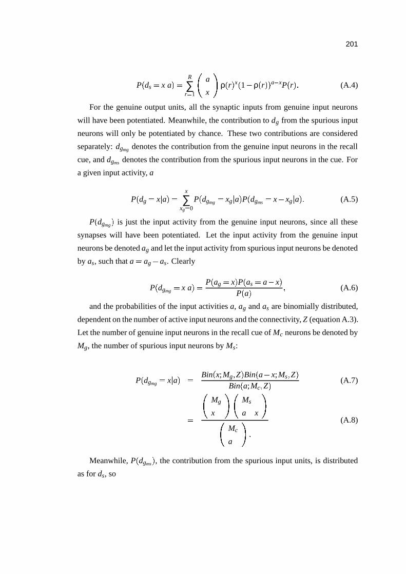
201
P � ds � x�a � � R
∑r � 1
�a
x � ρ � r � x � 1 � ρ � r � � a�
xP � r � � (A.4)
For the genuine output units, all the synaptic inputs from genuine input neurons
will have been potentiated. Meanwhile, the contribution to dg from the spurious input
neurons will only be potentiated by chance. These two contributions are considered
separately: dgmg denotes the contribution from the genuine input neurons in the recall
cue, and dgms denotes the contribution from the spurious input neurons in the cue. For
a given input activity, a
P � dg � x�a � � x
∑xg � 0
P � dgmg � xg�a � P � dgms � x � xg
�a � � (A.5)
P � dgmg � is just the input activity from the genuine input neurons, since all these
synapses will have been potentiated. Let the input activity from the genuine input
neurons be denoted ag and let the input activity from spurious input neurons be denoted
by as, such that a � ag�
as. Clearly
P � dgmg � x�a � � P � ag � x � P � as � a � x �
P � a � � (A.6)
and the probabilities of the input activities a, ag and as are binomially distributed,
dependent on the number of active input neurons and the connectivity, Z (equation A.3).
Let the number of genuine input neurons in the recall cue of Mc neurons be denoted by
Mg, the number of spurious input neurons by Ms:
P � dgmg � x�a � � Bin � x;Mg � Z � Bin � a � x;Ms � Z �
Bin � a;Mc � Z � (A.7)
��
Mg
x � �Ms
a � x ��Mc
a � �
(A.8)
Meanwhile, P � dgms � , the contribution from the spurious input units, is distributed
as for ds, so
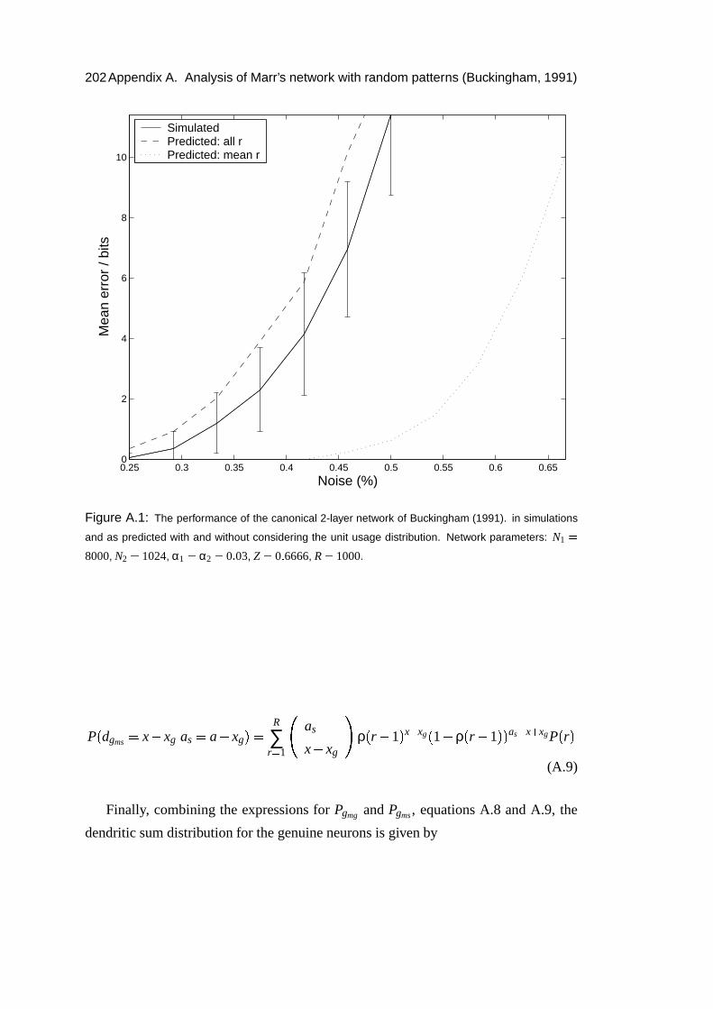
202Appendix A. Analysis of Marr’s network with random patterns (Buckingham, 1991)
0.25 0.3 0.35 0.4 0.45 0.5 0.55 0.6 0.650
2
4
6
8
10
Noise (%)
Mea
n er
ror
/ bits
SimulatedPredicted: all rPredicted: mean r
Figure A.1: The performance of the canonical 2-layer network of Buckingham (1991). in simulations
and as predicted with and without considering the unit usage distribution. Network parameters: N1 �
8000, N2 � 1024, α1 � α2 � 0 � 03, Z � 0 � 6666, R � 1000.
P � dgms � x � xg�as � a � xg � � R
∑r � 1
�as
x � xg � ρ � r � 1 � x�
xg � 1 � ρ � r � 1 � � as�
x � xgP � r �(A.9)
Finally, combining the expressions for Pgmg and Pgms , equations A.8 and A.9, the
dendritic sum distribution for the genuine neurons is given by
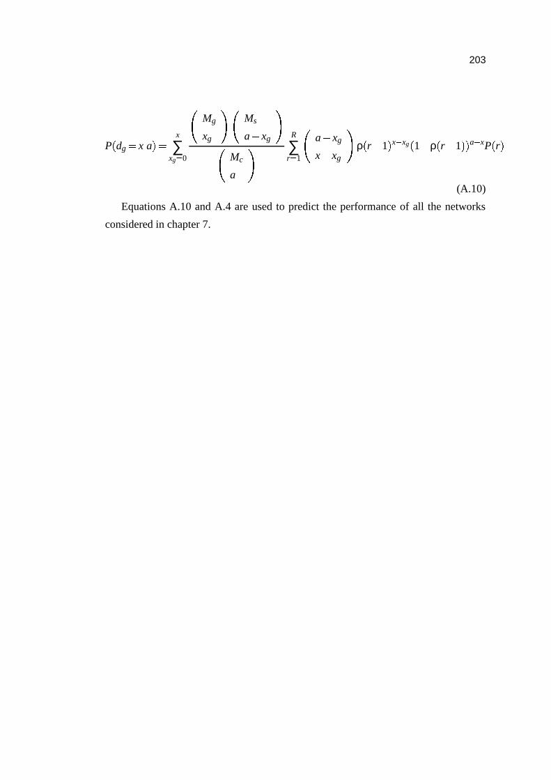
203
P � dg � x�a � � x
∑xg � 0
�Mg
xg � �Ms
a � xg ��Mc
a �R
∑r � 1
�a � xg
x � xg � ρ � r � 1 � x�
xg � 1 � ρ � r � 1 � � a�
xP � r �
(A.10)
Equations A.10 and A.4 are used to predict the performance of all the networks
considered in chapter 7.


Appendix B
Analysis of Marr’s self-organising
network (Buckingham, 1991)
The output neurons are selected because they have the highest connectivity for that
pattern. Marr calculates the effective connectivity, denoted by Zg, as proportion of the
total number of active input synapses (over all the output neurons) out of the largest
possible number of input synapses, M1� M2:
Zg �N2
M1
∑a � T
B � a;M1 � Z � aM1M2
� (B.1)
where T is the threshold on the input activity, a, used during pattern formation
(Marr, 1971, sec. 3.1.3.S2). Buckingham (1991, sec. 5.2) believes Marr’s expression
to be unargued and suggests
Zg �M1
∑a � T
B � a;M1 � Z � a
M1
M1
∑a � � T
B � a �
;M1 � Z �� (B.2)
but since
205
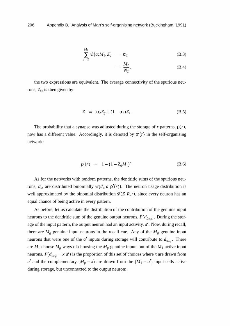
206 Appendix B. Analysis of Marr’s self-organising network (Buckingham, 1991)
M1
∑a � T
B � a;M1 � Z � � α2 (B.3)
� M2
N2� (B.4)
the two expressions are equivalent. The average connectivity of the spurious neu-
rons, Zs, is then given by
Z � α2Zg� � 1 � α2 � Zs � (B.5)
The probability that a synapse was adjusted during the storage of r patterns, ρ � r � ,now has a different value. Accordingly, it is denoted by ρ
� � r � in the self-organising
network:
ρ� � r � � 1 � � 1 � ZgM1 � r � (B.6)
As for the networks with random patterns, the dendritic sums of the spurious neu-
rons, ds, are distributed binomially B � ds;a � ρ� � r � � . The neuron usage distribution is
well approximated by the binomial distribution B � Z � R � r � , since every neuron has an
equal chance of being active in every pattern.
As before, let us calculate the distribution of the contribution of the genuine input
neurons to the dendritic sum of the genuine output neurons, P � dgmg � . During the stor-
age of the input pattern, the output neuron had an input activity, a�
. Now, during recall,
there are Mg genuine input neurons in the recall cue. Any of the Mg genuine input
neurons that were one of the a�
inputs during storage will contribute to dgmg . There
are M1 choose Mg ways of choosing the Mg genuine inputs out of the M1 active input
neurons. P � dgmg � x�a
� � is the proportion of this set of choices where x are drawn from
a�
and the complementary � Mg � x � are drawn from the � M1 � a� � input cells active
during storage, but unconnected to the output neuron:

207
P � dgmg � x�a
� � ��
a�
x � �M1 � a
�
mg � x ��M1
mg � � (B.7)
Averaging P � dgmg � x�a
� � over P � a � � gives an accurate approximation to P � dgmg � :
P � dgmg � x � � M1
∑a � � T
P � dgmg � x�a
� � B � a �
;M1 � Z � (B.8)
contrary to the formula given by Buckingham (1991, page 141).
During recall, the output neuron will have an input activity, a, distinct from the
input activity during storage, a�
. Of the a active inputs, ag are genuine and as are
spurious. All ag will have been modified, so the distribution of ag is P � dgmg � , while as
is binomially distributed, dependent on Ms and Zs:
P � a � � min�a �mg �∑
ag � 0P � ag � P � as � a � ag � (B.9)
� min�a �mg �∑
ag � 0P � dgmg � ag � B � a � ag;Ms � Zs � � (B.10)
Combining equations B.8 and B.9,
P � dgmg � x�a � � P � dgmg � x � P � as � a � x �
P � a � (B.11)
� P � dgmg � x � B � a � x;Ms � Zs �P � a � � (B.12)
As for the storage of random patterns, the contribution to the dendritic sum of the
genuine output neuron from spurious input neurons, ds, is distributed B � ds;as � ρ � r �
1 � � . Combining P � ds � with equation B.11, and averaging over all dgmg and r,
P � dg � x�a � � x
∑xg � 0
P � dgmg � xg�a � P � dgms � x � xg
�a � (B.13)
� x
∑xg � 0
P � dgmg � xg�a �
R
∑r � 0
B � x � xg;a � xg � ρ� � r � 1 � � P � r � � (B.14)
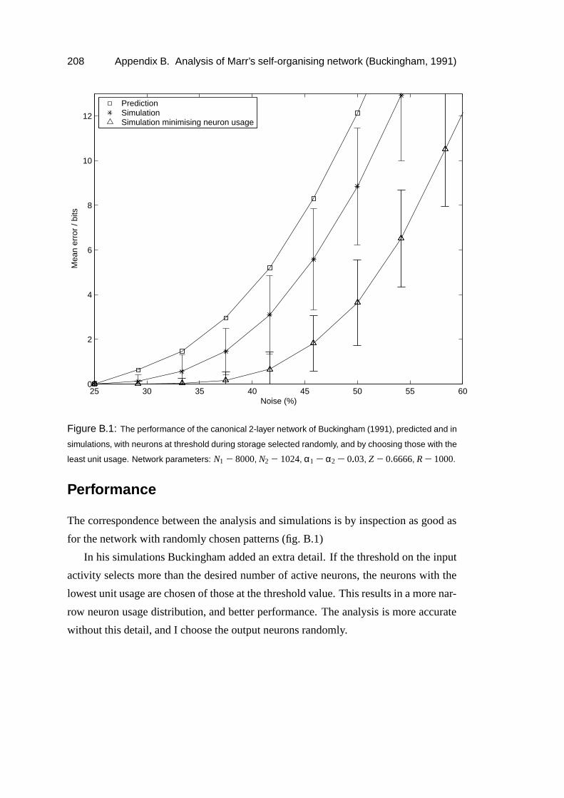
208 Appendix B. Analysis of Marr’s self-organising network (Buckingham, 1991)
25 30 35 40 45 50 55 600
2
4
6
8
10
12
Noise (%)
Mea
n er
ror
/ bits
PredictionSimulationSimulation minimising neuron usage
Figure B.1: The performance of the canonical 2-layer network of Buckingham (1991), predicted and in
simulations, with neurons at threshold during storage selected randomly, and by choosing those with the
least unit usage. Network parameters: N1 � 8000, N2 � 1024, α1 � α2 � 0 � 03, Z � 0 � 6666, R � 1000.
Performance
The correspondence between the analysis and simulations is by inspection as good as
for the network with randomly chosen patterns (fig. B.1)
In his simulations Buckingham added an extra detail. If the threshold on the input
activity selects more than the desired number of active neurons, the neurons with the
lowest unit usage are chosen of those at the threshold value. This results in a more nar-
row neuron usage distribution, and better performance. The analysis is more accurate
without this detail, and I choose the output neurons randomly.
Bibliography
Abbott, L. and Blum, K. (1996). Functional significance of long-term potentiation for
sequence learning and prediction. Cerebral Cortex, 6(3):406–16.
Agnihotri, N., Hawkins, R., Kandel, E., and Kentros, C. (2004). The long-term stability
of new hippocampal place fields requires new protein synthesis. Proceedings of
the National Academy of Sciences, U.S.A., 101(10):3656–61.
Alle, H., Jonas, P., and Geiger, J. (2001). PTP and LTP at a hippocampal mossy fiber-
interneuron synapse. Proceedings of the National Academy of Sciences, U.S.A.,
98(25):14708–13.
Alvarez, P. and Squire, L. (1994). Memory consolidation and the medial temporal
lobe: a simple network model. Proceedings of the National Academy of Science,
U.S.A., 91(15):7041–5.
Amaral, D. (1993). Emerging principles of intrinsic hippocampal organization. Cur-
rent Opinion in Neurobiology, 3(2):225–9.
Amaral, D., Dolorfo, C., and Alvarez-Royo, P. (1991). Organization of CA1 projec-
tions to the subiculum: a PHA-L analysis in the rat. Hippocampus, 1(4):415–35.
Amaral, D., Ishizuka, N., and Claiborne, B. (1990). Neurons, numbers and the hip-
pocampal network. Progress in Brain Research, 83:1–11.
Amaral, D. and Witter, M. (1989). The three-dimensional organization of the hip-
pocampal formation: a review of anatomical data. Neuroscience, 31(3):571–91.
209
210 Bibliography
Amaral, D. and Witter, M. (1995). The Rat Nervous System, chapter Hippocampal
formation, pages 443–494. Academic Press, San Diego, New York, 2nd edition.
Andersen, P., Bliss, V., and Skrede, K. (1971). Lamellar organization of hippocampal
excitatory pathways. Experimental Brain Research, 13(2):222–238.
Aranzi, G. (1564). De humano foetu opusculum. Rome.
Arleo, A. and Gerstner, W. (2000). Spatial cognition and neuro-mimetic navigation: a
model of hippocampal place cell activity. Biological Cybernetics, 83(3):287–99.
Arolfo, M., Nerad, L., Schenk, F., and Bures, J. (1994). Absence of snapshot memory
of the target view interferes with place navigation learning by rats in the water
maze. Behavioral Neuroscience, 108(2):308–16.
Arrigoni, E. and Greene, R. (2004). Schaffer collateral and perforant path inputs ac-
tivate different subtypes of NMDA receptors on the same CA1 pyramidal cell.
British Journal of Pharmacology, 142(2):317–22.
Barbarosie, M., Louvel, J., Kurcewicz, I., and Avoli, M. (2000). CA3-Released
entorhinal seizures disclose dentate gyrus epileptogenicity and unmask a tem-
poroammonic pathway. Journal of Neurophysiology, 83(3):1115–24.
Barnes, C., McNaughton, B., Mizumori, S., Leonard, B., and Lin, L. (1990). Com-
parison of spatial and temporal characteristics of neuronal activity in sequential
stages of hippocampal processing. Progress in Brain Research, 83:287–300.
Bartesaghi, R. and Gessi, T. (2003). Activation of perforant path neurons to field CA1
by hippocampal projections. Hippocampus, 2:235–49.
Battaglia, F. and Treves, A. (1998). Attractor neural networks storing multiple space
representations: A model for hippocampal place fields. Physical Review E,
58(6):7738–7753. Part B.
Bennet, M., Gibson, W., and Robinson, J. (1994). Dynamics of the CA3 pyramidal
neuron associative memory network in the hippocampus. Philosophical Transac-
tions of the Royal Society B, 343:167–187.
Bibliography 211
Best, P., White, A., and Minai, A. (2001). Spatial processing in the brain: the activity
of hippocampal place cells. Annual Review of Neuroscience, 24:459–86.
Bezzi, M., Samengo, I., Leutgeb, S., and Mizumori, S. (2002). Measuring information
spatial densities. Neural Computation, 14(2):405–20.
Bi, G. and Poo, M. (1998). Synaptic modifications in cultured hippocampal neurons:
Dependence on spike timing, synaptic strength, and postsynaptic cell type. Jour-
nal of Neuroscience, 18(24):10464–72.
Biegler, R. and Morris, R. (1999). Blocking in the spatial domain with arrays of dis-
crete landmarks. Journal of Experimental Psychology: Animal Behavior Pro-
cesses, 25(3):334–51.
Bienenstock, E., Cooper, L., and Munro, P. (1982). Theory for the development of neu-
ron selectivity: orientation specificity and binocular interaction in visual cortex.
Journal of Neuroscience, 2(1):32–48.
Blackstad, T. (1956). Commissural connections of the hippocampal region in the rat,
with special reference to their mode of termination. Journal of Comparative Neu-
rology, 105:417–537.
Blasco-Ibanez, J. and Freund, T. (1995). Synaptic input of horizontal interneurons in
stratum oriens of the hippocampal CA1 subfield: structural basis of feed-back
activation. European Journal of Neuroscience, 7(10):2170–80.
Bliss, T. V. and Collingridge, G. L. (1993). A synaptic model of memory: long-term
potentiation in the hippocampus. Nature, 361(6407):31–9.
Bogacz, R., Brown, M., and Giraud-Carrier, C. (2001). Model of familiarity discrimi-
nation in the perirhinal cortex. Journal of Computational Neuroscience, 10(1):5–
23.
Bostock, E., Muller, R., and Kubie, J. (1991). Experience-dependent modifications of
hippocampal place cell firing. Hippocampus, 1(2):193–205.
212 Bibliography
Brankack, J., Stewart, M., and Fox, S. (1993). Current source density analysis of the
hippocampal theta rhythm: associated sustained potentials and candidate synaptic
generators. Brain Research, 615(2):310–27.
Brindley, G. (1969). Nerve net models of plausible size that perform many simple
learning tasks. Proceedings of the Royal Society of London B, Biological Sciences,
174(35):173–91.
Brown, M. and Aggleton, J. (2001). Recognition memory: what are the roles of the
perirhinal cortex and hippocampus? Nature Reviews Neuroscience, 2(1):51–61.
Brun, V., Otnass, M., Molden, S., Steffenach, H., Witter, M., Moser, M., and Moser,
E. (2002). Place cells and place recognition maintained by direct entorhinal-
hippocampal circuitry. Science, 296(5576):2243–6.
Brunel, N. and Trullier, O. (1998). Plasticity of directional place fields in a model of
rodent CA3. Hippocampus, 8(6):651–65.
Buckingham, J. (1991). Delicate nets, faint recollections: a study of partially con-
nected associative network memories. PhD thesis, University of Edinburgh.
Buckingham, J. and Willshaw, D. (1992). Performance characteristics of the associa-
tive net. Network, 3:407–414.
Buckingham, J. and Willshaw, D. (1993). On setting unit thresholds in an incompletely
connected associative net. Network, 4:441–459.
Buhl, E., Cobb, S., Halasy, K., and Somogyi, P. (1995). Properties of unitary IPSPs
evoked by anatomically identified basket cells in the rat hippocampus. European
Journal of Neuroscience, 7(9):1989–2004.
Buhusi, C. and Schmajuk, N. (1996). Attention, configuration, and hippocampal func-
tion. Hippocampus, 6(6):621–42.
Bures, J., Fenton, A., Kaminsky, Y., and Zinyuk, L. (1997). Place cells and place
navigation. Proceedings of the National Academy of Sciences, U.S.A., 94(1):343–
50.
Bibliography 213
Burgess, N. and O’Keefe, J. (1996). Neuronal computations underlying the firing of
place cells and their role in navigation. Hippocampus, 6(6):749–62.
Burgess, N., Recce, M., and O’Keefe, J. (1994). A model of hippocampal function.
Neural Networks, 7:1065–81.
Burwell, R. (2000). The parahippocampal region: corticocortical connectivity. Annals
of the New York Academy of Sciences, 911:25–42.
Burwell, R., Shapiro, M., O’Malley, M., and Eichenbaum, H. (1998). Positional firing
properties of perirhinal cortex neurons. Neuroreport, 9(13):3013–8.
Buzsaki, G. (1989). Two-stage model of memory trace formation: a role for ”noisy”
brain states. Neuroscience, 31(3):551–70.
Buzsaki, G., Penttonen, M., Bragin, A., Nadasdy, Z., and Chrobak, J. (1995). Possible
physiological role of the perforant path-CA1 projection. Hippocampus, 5:141–
146.
Canning, A. and Gardner, E. (1988). Partially connected models of neural networks.
Journal of Physics A: Mathematical and General, 21:3275–84.
Canning, K., Wu, K., Peloquin, P., Kloosterman, F., and Leung, L. (2000). Physiology
of the entorhinal and perirhinal projections to the hippocampus studied by current
source density analysis. Annals of the New York Academy of Sciences, 911:55–72.
Christie, B., Franks, K., Seamans, J., Saga, K., and Sejnowski, T. (2000). Synaptic
plasticity in morphologically identified CA1 stratum radiatum interneurons and
giant projection cells. Hippocampus, 10(6):673–83.
Clayton, N. and Dickinson, A. (1998). Episodic-like memory during cache recovery
by scrub jays. Nature, 395(6699):272–4.
Clayton, N., Yu, K., and Dickinson, A. (2003). Interacting cache memories: evidence
for flexible memory use by Western Scrub-Jays (Aphelocoma californica). Jour-
nal of Experimental Psychology: Animal Behavior Processes, 29(1):14–22.
214 Bibliography
Cohen, N. and Eichenbaum, H. (1993). Memory, amnesia, and the hippocampal sys-
tem. The MIT press, Cambridge, Massachusetts.
Colbert, C. and Levy, W. (1992). Electrophysiological and pharmacological charac-
terization of perforant path synapses in CA1: mediation by glutamate receptors.
Journal of Neurophysiology, 68(1):1–8.
Colbert, C. and Levy, W. (1993). Long-term potentiation of perforant path synapses in
hippocampal CA1 in vitro. Brain Research, 606(1):87–91.
Corkin, S. (1968). Acquisition of motor skill after bilateral medial temporal-lobe ex-
cision. Neuropsychologia, 6(3):255–265.
Csicsvari, J., Hirase, H., Czurko, A., and Buzsaki, G. (1998). Reliability and state
dependence of pyramidal cell-interneuron synapses in the hippocampus: an en-
semble approach in the behaving rat. Neuron, 21(1):179–89.
Davies, C., Starkey, S., Pozza, M., and Collingridge, G. (1991). GABA autoreceptors
regulate the induction of LTP. Nature, 349(6310):609–11.
Day, M., Langston, R., and Morris, R. (2003). Glutamate-receptor-mediated encoding
and retrieval of paired-associate learning. Nature, 424(6945):205–9.
Dayan, P. and Willshaw, D. (1991). Optimizing synaptic learning rules in linear asso-
ciative memories. Biological Cybernetics, 65(4):253–265.
de Hoz, L., Knox, J., and Morris, R. (2003). Longitudinal axis of the hippocampus:
both septal and temporal poles of the hippocampus support water maze spatial
learning depending on the training protocol. Hippocampus, 13(5):587–603.
Deadwyler, S., West, J., Cotman, C., and Lynch, G. (1975). Physiological studies
of the reciprocal connections between the hippocampus and entorhinal cortex.
Experimental Neurology, 49(1 Pt 1):35–57.
Delatour, B. and Witter, M. (2002). Projections from the parahippocampal region to
the prefrontal cortex in the rat: evidence of multiple pathways. European Journal
of Neuroscience, 15(8):1400–7.
Bibliography 215
Deuchars, J. and Thomson, A. (1996). CA1 pyramid-pyramid connections in rat hip-
pocampus in vitro: dual intracellular recordings with biocytin filling. Neuro-
science, 74(4):1009–18.
Doller, H. and Weight, F. (1982). Perforant pathway activation of hippocampal CA1
stratum pyramidale neurons: electrophysiological evidence for a direct pathway.
Brain Research, 237(1):1–13.
Doller, H. and Weight, F. (1985). Perforant pathway-evoked long-term potentiation of
CA1 neurons in the hippocampal slice preparation. Brain Research, 333(2):305–
310.
Dolorfo, C. and Amaral, D. (1998a). Entorhinal cortex of the rat: topographic organi-
zation of the cells of origin of the perforant path projection to the dentate gyrus.
Journal of Comparative Neurology, 398(1):25–48.
Dolorfo, C. and Amaral, D. (1998b). Entorhinal cortex of the rat: topographic organi-
zation of the cells of origin of the perforant path projection to the dentate gyrus.
Journal of Comparative Neurology, 398(1):25–48.
Dvorak-Carbone, H. and Schuman, E. (1999a). Long-term depression of
temporoammonic-CA1 hippocampal synaptic transmission. Journal of Neuro-
physiology, 81:1036–1044.
Dvorak-Carbone, H. and Schuman, E. (1999b). Patterned activity in stratum lacuno-
sum moleculare inhibits CA1 pyramidal neuron firing. Journal of Neurophysiol-
ogy, 82:3213–3222.
Eichenbaum, H. (2001). The hippocampus and declarative memory: cognitive mecha-
nisms and neural codes. Behavioral Brain Research, 127(1-2):199–207.
Eichenbaum, H., Dudchenko, P., Wood, E., Shapiro, M., and Tanila, H. (1999). The
hippocampus, memory, and place cells: is it spatial memory or a memory space?
Neuron, 23(2):209–26.
216 Bibliography
Ekstrom, A., Meltzer, J., McNaughton, B., and Barnes, C. (2001). NMDA receptor an-
tagonism blocks experience-dependent expansion of hippocampal ”place fields”.
Neuron, 31(4):631–8.
Empson, R. and Heinemann, U. (1995). The perforant path projection to hippocampal
area CA1 in the rat hippocampal-entorhinal cortex combined slice. Journal of
Physiology, 484:707–20.
Ferbinteanu, J. and Shapiro, M. (2003). Prospective and retrospective memory coding
in the hippocampus. Neuron, 40(6):1227–39.
Fortin, N., Agster, K., and Eichenbaum, H. (2002). Critical role of the hippocampus
in memory for sequences of events. Nature Neuroscience, 5(5):458–62.
Foster, D., Morris, R., and Dayan, P. (2000). A model of hippocampally dependent
navigation, using the temporal difference learning rule. Hippocampus, 10(1):1–
16.
Frank, L., Brown, E., and Wilson, M. (2000). Trajectory encoding in the hippocampus
and entorhinal cortex. Neuron, 27(1):169–78.
Frank, L., Brown, E., and Wilson, M. (2001). A comparison of the firing properties
of putative excitatory and inhibitory neurons from CA1 and the entorhinal cortex.
Journal of Neurophysiology, 86(4):2029–2040.
Frank, L., Eden, U., Solo, V., Wilson, M., and Brown, E. (2002). Contrasting pat-
terns of receptive field plasticity in the hippocampus and the entorhinal cortex: an
adaptive filtering approach. Journal of Neuroscience, 22(9):3817–30.
Freund, T. and Buzsaki, G. (1996). Interneurons of the hippocampus. Hippocampus,
6:347–470.
Frey, U. and Morris, R. (1998). Synaptic tagging: implications for late maintenance of
hippocampal long-term potentiation. Trends in Neuroscience, 21(5):181–8.
Bibliography 217
Fricker, D., Verheugen, J., and Miles, R. (1999). Cell-attached measurements of the fir-
ing threshold of rat hippocampal neurones. Journal of Physiology, 517(Pt 3):791–
804.
Frolov, A., Kartashov, A., Goltsev, A., and Folk, R. (1995a). Quality and efficiency
of retrieval for Willshaw-like autoassociative networks. 1. Correction. Network:
Computation in Neural Systems, 6(4):513–34.
Frolov, A., Kartashov, A., Goltsev, A., and Folk, R. (1995b). Quality and efficiency
of retrieval for Willshaw-like autoassociative networks. 2. Recognition. Network:
Computation in Neural Systems, 6(4):535–49.
Fuhs, M. and Touretzky, D. (2000). Synaptic learning models of map separation in the
hippocampus. Neurocomputing, 32:379–384.
Fulvi-Mari, C., Panzeri, S., Rolls, E., and Treves, A. (1999). Information Theory and
the Brain, chapter 15, A quantitative model of information processing in CA1,
pages 273–289. Cambridge University Press.
Fyhn, M., Molden, S., Hollup, S., Moser, M., and Moser, E. (2002). Hippocampal
neurons responding to first-time dislocation of a target object. Neuron, 35(3):555–
66.
Fyhn, M., Witter, M., Moser, M., and Moser, E. (2003). Decorrelation of spatial
input from entorhinal cortex in dentate gyrus and hippocampus. In Society for
Neuroscience Abstracts.
Gaffan, D. (2002). Against memory systems. Philosophical Transactions of the Royal
Society of London B, Biological Sciences, 357(1424):1111–21.
Ganeshina, O., Berry, R., Petralia, R., Nicholson, D., and Geinisman, Y. (2004). Dif-
ferences in the expression of AMPA and NMDA receptors between axospinous
perforated and nonperforated synapses are related to the configuration and size of
postsynaptic densities. Journal of Comparative Neurology, 468(1):86–95.
218 Bibliography
Gardner-Medwin, A. (1976). The recall of events through the learning of associations
between their parts. Proceedings of the Royal Society of London B, Biological
Sciences, 194(1116):375–402.
Gaussier, P., Revel, A., Banquet, J., and Babeau, V. (2002). From view cells and place
cells to cognitive map learning: processing stages of the hippocampal system.
Biological Cybernetics, 86(1):15–28.
Gibson, W. and Robinson, J. (1992). Statistical analysis of the dynamics of a sparse
associative memory. Neural Networks, 5(4):645–661.
Gibson, W., Robinson, J., and Bennett, M. (1991). Probabilistic secretion of quanta in
the central nervous system: granule cell synaptic control of pattern separation and
activity regulation. Philosophical Transactions of the Royal Society B., Biological
Sciences, 332(1264):199–220.
Gilbert, P. and Kesner, R. (2002). Role of the rodent hippocampus in paired-associate
learning involving associations between a stimulus and a spatial location. Behav-
ioral Neuroscience, 116(1):63–71.
Gilbert, P., Kesner, R., and Lee, I. (2001). Dissociating hippocampal subregions: a
double dissociation between dentate gyrus and CA1. Hippocampus, 11:626–636.
Gloveli, T., Schmitz, D., Empson, R., Dugladze, T., and Heinemann, U. (1997a). Mor-
phological and electrophysiological characterization of layer III cells of the me-
dial entorhinal cortex of the rat. Neuroscience, 77(3):629–48.
Gloveli, T., Schmitz, D., Empson, R., and Heinemann, U. (1997b). Frequency-
dependent information flow from the entorhinal cortex to the hippocampus. Jour-
nal of Neurophysiology, 78(6):3444–9.
Gluck, M. and Myers, C. (1993). Hippocampal mediation of stimulus representation:
a computational theory. Hippocampus, 3(4):491–516.
Gomez-Isla, T., Price, J., McKeel, D. J., J.C., M., Growdon, J., and Hyman, B.
(1996). Profound loss of layer II entorhinal cortex neurons occurs in very mild
Alzheimer’s disease. Journal of Neuroscience, 16(14):4491–500.
Bibliography 219
Graham, B. (2001). Pattern recognition in a compartmental model of a CA1 pyramidal
neuron. Network: Computation in Neural Systems, 12(4):473–92.
Graham, B. and Willshaw, D. (1995). Improving recall from an associative memory.
Biological Cybernetics, 72:337–346.
Graham, B. and Willshaw, D. (1999). Probabilistic synaptic transmission in the asso-
ciative net. Neural Computation, 11(1):117–37.
Granger, R., Whitson, J., Larson, J., and Lynch, G. (1994). Non-hebbian properties
of long-term potentiation enable high-capacity encoding of temporal sequences.
Proceedings of the National Academy of Science, U.S.A., 91(21):10104–8.
Gulyas, A., Megias, M., Emri, Z., and Freund, T. (1999). Total number and ratio
of excitatory and inhibitory synapses converging onto single interneurons of dif-
ferent types in the CA1 area of the rat hippocampus. Journal of Neuroscience,
19(22):10082–97.
Hampson, R. and Deadwyler, S. (2003). Temporal firing characteristics and the strate-
gic role of subicular neurons in short-term memory. Hippocampus, 13(4):529–41.
Hampson, R., Hedberg, T., and Deadwyler, S. (2000). Differential information pro-
cessing by hippocampal and subicular neurons. Annals of the New York Academy
of Sciences, 911:151–165.
Harris, E. and Stewart, M. (2001). Intrinsic connectivity of the rat subiculum: II.
Properties of synchronous spontaneous activity and a demonstration of multiple
generator regions. Journal of Comparative Neurology, 435(4):506–18.
Harris, E., Witter, M., Weinstein, G., and Stewart, M. (2001). Intrinsic connectivity
of the rat subiculum: I. Dendritic morphology and patterns of axonal arborization
by pyramidal neurons. Journal of Comparative Neurology, 435(4):490–505.
Hartley, T., Burgess, N., Lever, C., Cacucci, F., and O’Keefe, J. (2000). Modeling
place fields in terms of the cortical inputs to the hippocampus. Hippocampus,
10(4):369–79.
220 Bibliography
Hasselmo, M., Bodelon, C., and Wyble, B. (2002). A proposed function for hippocam-
pal theta rhythm: separate phases of encoding and retrieval enhance reversal of
prior learning. Neural Computation, 14(4):793–817.
Hasselmo, M. and Bower, J. (1992). Cholinergic suppression specific to intrinsic not
afferent fiber synapses in rat piriform (olfactory) cortex. Journal of Neurophysi-
ology, 67(5):1222–9.
Hasselmo, M. and Schnell, E. (1994). Laminar selectivity of the cholinergic sup-
pression of synaptic transmission in rat hippocampal region CA1: computational
modeling and brain slice physiology. Journal of Neuroscience, 14(6):3898–914.
Hasselmo, M., Wyble, B., and Wallenstein, G. (1996). Encoding and retrieval of
episodic memories: role of cholinergic and gabaergic modulation in the hip-
pocampus. Hippocampus, 6(6):693–708.
Hayman, R., Chakraborty, S., Anderson, M., and Jeffery, K. (2003). Context-specific
acquisition of location discrimination by hippocampal place cells. European Jour-
nal of Neuroscience, 18(10):2825–34.
Hebb, D. (1949). The Organization of Behaviour. New York: Wiley.
Heinemann, U., Schmitz, D., Eder, C., and Gloveli, T. (2000). Properties of entorhinal
cortex projection cells to the hippocampal formation. Annuals of the New York
Academy of Sciences, 911:1112–26.
Hess, U., Lynch, G., and Gall, C. (1995). Regional patterns of c-fos mRNA expression
in rat hippocampus following exploration of a novel environment versus perfor-
mance of a well-learned discrimination. Journal of Neuroscience, 15(12):7796–
809.
Hetherington, P. and Shapiro, M. (1993). A simple network model simulates hip-
pocampal place fields: II. Computing goal-directed trajectories and memory
fields. Behavioral Neuroscience, 107(3):434–43.
Bibliography 221
Hille, B. (2001). Ion Channels of Excitable Membranes. Sinauer Associates, Inc., third
edition.
Hirase, H. and Recce, M. (1995). Performance analysis of progressive recall in par-
tially connected recurrent networks. In Fogelman-Soulie, F. and Gallinari, P., ed-
itors, Proceedings of the International Conference on Artificial Neural Networks
(ICANN’95), pages 509–14. Paris: EC2.
Hirase, H. and Recce, M. (1996). A search for the optimal thresholding sequence in
an associative memory. Network: Computation in Neural Systems, 7(4):741–56.
Holscher, C., Anwyl, R., and Rowan, M. (1997). Stimulation on the positive phase
of hippocampal theta rhythm induces long-term potentiation that can be depo-
tentiated by stimulation on the negative phase in area CA1 in vivo. Journal of
Neuroscience, 17(16):6470–7.
Holt, G. and Koch, C. (1997). Shunting inhibition does not have a divisive effect on
firing rates. Neural Computation, 9(5):1001–13.
Iijima, T., Witter, M., Ichikawa, M., Tominaga, T., Kajiwara, R., and Matsumoto,
G. (1996). Entorhinal-hippocampal interactions revealed by real-time imaging.
Science, 272(5265):1176–9.
Inoue, M., Mikami, A., Ando, I., and Tsukada, H. (2004). Functional brain mapping
of the macaque related to spatial working memory as revealed by PET. Cerebral
Cortex, 14(1):106–19.
Insausti, R., Herrero, M., and Witter, M. (1997). Entorhinal cortex of the rat: cy-
toarchitectonic subdivisions and the origin and distribution of cortical efferents.
Hippocampus, 7(2):146–83.
Isaac, J., Nicoll, R., and Malenka, R. (1995). Evidence for silent synapses: implica-
tions for the expression of LTP. Neuron, 15(2):427–34.
Ishizuka, N., Cowan, W., and Amaral, D. (1995). A quantitative analysis of the den-
dritic organization of pyramidal cells in the rat hippocampus. Journal of Compar-
ative Neurology, 362(1):17–45.
222 Bibliography
Ishizuka, N., Weber, J., and Amaral, D. (1990). Organization of intrahippocampal pro-
jections originating from CA3 pyramidal cells in the rat. Journal of Comparative
Neurology, 295(4):580–623.
Jakab, R. and Leranth, C. (1995). The rat nervous system, chapter Septum, pages
405–442. San Diego: Academic Press, 2nd edition.
Jeffery, K., Anderson, M., Hayman, R., and Chakraborty, S. (2004). A proposed archi-
tecture for the neural representation of spatial context. Neuroscience Behavioral
Reviews, 28(2):201–18.
Jeffery, K., Gilbert, A., Burton, S., and Strudwick, A. (2003). Preserved performance
in a hippocampal-dependent spatial task despite complete place cell remapping.
Hippocampus, 13(2):175–89.
Jung, M. and McNaughton, B. (1993). Spatial selectivity of unit activity in the hip-
pocampal granular layer. Hippocampus, 3(2):165–82.
Jung, M., Wiener, S., and McNaughton, B. (1994). Comparison of spatial firing char-
acteristics of units in dorsal and ventral hippocampus of the rat. Journal of Neu-
roscience, 14(12):7347–56.
Kahana, M., Seelig, D., and Madsen, J. (2001). Theta returns. Current Opinion in
Neurobiology, 11(6):739–44.
Kali, S. and Dayan, P. (2000). The involvement of recurrent connections in area CA3
in establishing the properties of place fields: a model. Journal of Neuroscience,
20(19):7463–77.
Kali, S. and Dayan, P. (2004). Off-line replay maintains declarative memories in a
model of hippocampal-neocortical interactions. Nature Neuroscience, 7(3):286–
94.
Kensinger, E., Ullman, M., and Corkin, S. (2001). Bilateral medial temporal lobe
damage does not affect lexical or grammatical processing: evidence from amnesic
patient H.M. Hippocampus, 11(4):347–60.
Bibliography 223
Kentros, C., Agnihotri, N., Streater, S., Hawkins, R., and Kandel, E. (2004). Increased
attention to spatial context increases both place field stability and spatial memory.
Neuron, 42(2):283–95.
Kentros, C., Hargreaves, E., Hawkins, R., Kandel, E., Shapiro, M., and Muller, R.
(1998). Abolition of long-term stability of new hippocampal place cell maps by
NMDA receptor blockade. Science, 280(5372):2121–6.
Kesner, R. and Novak, J. (1982). Serial position curve in rats: role of the dorsal
hippocampus. Science, 218(4568):173–5.
Kiss, J., Buzsaki, G., Morrow, J., Glantz, S., and Leranth, C. (1996). Entorhinal corti-
cal innervation of parvalbumin-containing neurons (Basket and Chandelier cells)
in the rat Ammon’s horn. Hippocampus, 6(3):239–46.
Klausberger, T., Magill, P., Marton, L., Roberts, J., Cobden, P., Buzsaki, G., and Som-
ogyi, P. (2003). Brain-state- and cell-type-specific firing of hippocampal interneu-
rons in vivo. Nature, 421(6925):844–8.
Koene, R., Gorchetchnikov, A., Cannon, R., and Hasselmo, M. (2003). Modeling
goal-directed spatial navigation in the rat based on physiological data from the
hippocampal formation. Neural Networks, 16(5-6):577–84.
Kubie, J., Muller, R., and Bostock, E. (1990). Spatial firing properties of hippocampal
theta cells. Journal of Neuroscience, 10(4):110–23.
Lacaille, J. and Schwartzkroin, P. (1988). Stratum lacunosum-moleculare interneurons
of hippocampal CA1 region. I. Intracellular response characteristics, synaptic re-
sponses, and morphology. Journal of Neuroscience, 8(4):1400–10.
Lapicque, L. (1907). Recherches quantatives sur l’excitation electrique des nerfs traitee
comme une polarization. J. Physiol. Pathol. Gen., 9:620–635.
Lassalle, J.-M., Bataille, T., and Halley, H. (2000). Reversible inactivation of the
hippocampal mossy fiber synapses in mice impairs spatial learning, but neither
consolidation nor memory retrieval, in the Morris navigation task. Neurobiology
of Learning and Memory, 73(3):243–257.
224 Bibliography
Lee, I., Yoganarasimha, D. ., Rao, G., and Knierim, J. (2003). Differential coherence
of CA1 vs. CA3 place field ensembles in cue-conflict environments. In Society
for Neuroscience Abstracts.
Lei, S. and McBain, C. (2004). Two loci of expression for long-term depression
at hippocampal mossy fiber-interneuron synapses. Journal of Neuroscience,
24(9):2112–21.
Lenck-Santini, P., Muller, R., Save, E., and Poucet, B. (2002). Relationships between
place cell firing fields and navigational decisions by rats. Journal of Neuroscience,
22(20):9035–47.
Leung, L. (1995). Simulation of perforant path evoked field and intracellular potentials
in hippocampal CA1 area. Hippocampus, 5(2):129–36.
Leutgeb, S., Kjelstrup, K., Treves, A., Moser, M., and Moser, E. (2003). Differential
representation of context in hippocampal areas CA3 and CA1. In Society for
Neuroscience Abstracts.
Leutgeb, S. and Mizumori, S. (2002). Context-specific spatial representations by lat-
eral septal cells. Neuroscience, 112(3):655–63.
Lever, C., Wills, T., Cacucci, F., Burgess, N., and O’Keefe, J. (2002). Long-term
plasticity in hippocampal place-cell representation of environmental geometry.
Nature, 416(6876):90–4.
Levy, W. (1989). Computational models of learning in simple neural systems, chapter
A computational approach to hippocampal function, pages 243–305. Academic
Press, New York.
Levy, W. (1996). A sequence predicting CA3 is a flexible associator that learns and
uses context to solve hippocampal-like tasks. Hippocampus, 6:579–590.
Levy, W., Colbert, C., and Desmond, N. (1995). Another network model bites the
dust: entorhinal inputs are no more than weakly excitatory in the hippocampal
CA1 region. Hippocampus, 5:137–140.
Bibliography 225
Levy, W., Desmond, N., and Zhang, D. (1998). Perforant path activation modulates
the induction of long-term potentiation of the Schaffer collateral-hippocampal
CA1 response: theoretical and experimental analyses. Learning and Memory,
4(6):510–8.
Lorincz, A. (1998). Forming independent components via temporal locking of re-
construction architectures: a functional model of the hippocampus. Biological
Cybernetics, 79(3):263–75.
Lorincz, A. and Buzsaki, G. (2000). Two-phase computational model training long-
term memories in the entorhinal-hippocampal region. Annuals of the New York
Academy of Sciences, 911:83–111.
Li, S., Cullen, W., Anwyl, R., and Rowan, M. (2003). Dopamine-dependent facilitation
of LTP induction in hippocampal CA1 by exposure to spatial novelty. Nature
Neuroscience.
Li, X., Somogyi, P., Tepper, J., and Buzsaki, G. (1992). Axonal and dendritic ar-
borization of an intracellularly labeled chandelier cell in the CA1 region of rat
hippocampus. Experimental Brain Research, 90(3):519–25.
Li, X., Somogyi, P., Ylinen, A., and Buzsaki, G. (1994). The hippocampal CA3 net-
work: an in vivo intracellular labeling study. Journal of Comparative Neurology,
339(2):181–208.
Lisman, J. (1999). Relating hippocampal circuitry to function: recall of memory se-
quences by reciprocal dentate-CA3 interactions. Neuron, 22(3):233–42.
Lisman, J. and Idiart, M. (1995). Storage of 7 +/- 2 short-term memories in oscillatory
subcycles. Science, 267(5203):1512–5.
Lisman, J. and Otmakhova, N. (2001). Storage, recall, and novelty detection of se-
quences by the hippocampus: elaborating on the SOCRATIC model to account
for normal and aberrant effects of dopamine. Hippocampus, 11(5):551–68.
226 Bibliography
Liu, L., Wong, T., Pozza, M., Lingenhoehl, K., Wang, Y., Sheng, M., Auberson, Y.,
and Wang, Y. (2004). Role of NMDA receptor subtypes in governing the direction
of hippocampal synaptic plasticity. Science, 304(5673):1021–4.
Longden, K. and Willshaw, D. (2002). An evaluation of recurrent feedforward memory
networks and their relevance to the hippocampus. Neurocomputing, 44:527–31.
Lorente de No, R. (1933). Studies on the structure of the cerebral cortex. Journal fur
Psychologie und Neurologie, 45:381–438.
Lorente de No, R. (1934). Studies on the structure of the cerebral cortex. II. Continua-
tion of the study of the ammonic system. Journal fur Psychologie und Neurologie,
46:113–77.
Maccaferri, G. and McBain, C. (1995). Passive propagation of LTD to stratum oriens-
alveus inhibitory neurons modulates the temporoammonic input to the hippocam-
pal CA1 region. Neuron, 15(1):137–45.
Markus, E., Qin, Y., Leonard, B., Skaggs, W., McNaughton, B., and Barnes, C. (1995).
Interactions between location and task affect the spatial and directional firing of
hippocampal neurons. Journal of Neuroscience, 15(11):7079–94.
Marr, D. (1969). A theory of cerebellar cortex. Journal of Physiology, 202(2):437–70.
Marr, D. (1971). Simple memory: a theory for archicortex. Philosophical Transactions
of the Royal Society B, Biological Sciences, 262(841):24–81.
McClelland, J. and Goddard, N. (1996). Considerations arising from a complemen-
tary learning systems perspective on hippocampus and neocortex. Hippocampus,
6:654–665.
McEntee, W. and Mair, R. (1990). The Korsakoff syndrome: a neurochemical perspec-
tive. Trends in Neuroscience, 13(8):340–4. Erratum in: Trends in Neuroscience.
1990, 13(11):446.

Bibliography 227
McHugh, T., Blum, K., Tsien, J., Tonegawa, S., and Wilson, M. (1996). Impaired
hippocampal representation of space in CA1-specific NMDAR1 knockout mice.
Cell, 87(7):1339–49.
McNaughton, B., Barnes, C., Meltzer, J., and Sutherland, R. (1989). Hippocam-
pal granule cells are necessary for normal spatial learning but not for spatially-
selective pyramidal cell discharge. Experimental Brain Research, 76(3):485–96.
McNaughton, B., Barnes, C., and O’Keefe, J. (1983). The contributions of position,
direction, and velocity to single unit activity in the hippocampus of freely-moving
rats. Experimental Brain Research, 52(1):41–9.
McNaughton, B. and Morris, R. (1987). Hippocampal synaptic enhancement and
information-storage within a distributed memory system. Trends in Neuroscience,
10(10):408–415.
Megıas, M., Emri, Z., Freund, T., and Gulyas, A. (2001). Total number and distribu-
tion of inhibitory and excitatory synapses on hippocampal CA1 pyramidal cells.
Neuroscience, 102(3):527–40.
Mehta, M., Barnes, C., and McNaughton, B. (1997). Experience-dependent, asymmet-
ric expansion of hippocampal place fields. Proceedings of the National Academy
of Sciences, U.S.A., 94:8918–8921.
Mehta, M., Quirk, M., and Wilson, M. (2000). Experience-dependent asymmetric
shape of hippocampal receptive fields. Neuron, 25:707–715.
Meunier, C., Yanai, H.-F., and Amari, S. (1991). Sparsely coded associative memories:
capacity and dynamical properties. Network: Computation in Neural Systems,
2:469–87.
Migliore, M. (2003). On the integration of subthreshold inputs from Perforant Path and
Schaffer Collaterals in hippocampal CA1 pyramidal neurons. Journal of Compu-
tational Neuroscience, 14(2):185–92.
228 Bibliography
Miles, R., Toth, K., Gulyas, A., Hajos, N., and Freund, T. (1996). Differences between
somatic and dendritic inhibition in the hippocampus. Neuron, 16(4):815–23.
Minai, A. (1997). Covariance learning of correlated patterns in competitive networks.
Neural Computation, 9(3):667–81.
Mizumori, S., McNaughton, B., Barnes, C., and Fox, K. (1989). Preserved spa-
tial coding in hippocampal CA1 pyramidal cells during reversible suppression
of CA3c output: evidence for pattern completion in hippocampus. Journal of
Neuroscience, 9:3915–3928.
Monyer, H., Burnashev, N., Laurie, D., Sakmann, B., and Seeburg, P. (1994). Devel-
opmental and regional expression in the rat brain and functional properties of four
NMDA receptors. Neuron, 12(3):529–40.
Morris, R. (2001). Episodic-like memory in animals: psychological criteria, neural
mechanisms and the value of episodic-like tasks to investigate animal models of
neurodegenerative disease. Philosophical Transactions of the Royal Society of
London B, Biological Sciences, 356(1413):1453–65.
Morris, R. and Frey, U. (1997). Hippocampal synaptic plasticity: role in spatial learn-
ing or the automatic recording of attended experience? Philosophical Transac-
tions of the Royal Society B, Biological Sciences, 352(1360):1489–1503.
Moser, M., Moser, E., Forrest, E., Andersen, P., and Morris, R. (1995). Spatial learning
with a minislab in the dorsal hippocampus. Proceedings of the National Academy
of Sciences, U.S.A., 92(21):9697–701.
Mott, D. and Lewis, D. (1991). Facilitation of the induction of long-term potentiation
by GABAB receptors. Science, 252(5013):1718–20.
Mulders, W., West, M., and Slomianka, L. (1997). Neuron numbers in the presubicu-
lum, parasubiculum, and entorhinal area of the rat. Journal of Comparative Neu-
rology, 385(1):83–94.
Muller, R. (1996). A quarter of a century of place cells. Neuron, 17(5):813–22.
Bibliography 229
Muller, R. and Kubie, J. (1987). The effects of changes in the environment on the
spatial firing of hippocampal complex-spike cells. Journal of Neuroscience,
7(7):1951–68.
Muller, R. and Stead, M. (1996). Hippocampal place cells connected by Hebbian
synapses can solve spatial problems. Hippocampus, 6(6):709–19.
Murre, J. (1996). TraceLink: a model of amnesia and consolidation of memory. Hip-
pocampus, 6(6):675–84.
Naber, P., da Silva, F., and Witter, M. (2001). Reciprocal connections between the
entorhinal cortex and hippocampal fields CA1 and the subiculum are in register
with the projections from CA1 to the subiculum. Hippocampus, 11(2):99–104.
Nadal, J.-P. and Toulouse, G. (1990). Information storage in sparsely coded memory
nets. Network: Computation in Neural Systems, 1:61–74.
Nadel, L. and Moscovitch, M. (1997). Memory consolidation, retrograde amnesia and
the hippocampal complex. Current Opinion in Neurobiology, 7(2):217–27.
Nadler, J., Perry, B., and Cotman, C. (1980). Selective reinnervation of hippocam-
pal area CA1 and the fascia dentata after destruction of CA3-CA4 afferents with
kainic acid. Brain Research, 182(1):1–9.
Nakazawa, K., McHugh, T., Wilson, M., and Tonegawa, S. (2004). NMDA recep-
tors, place cells and hippocampal spatial memory. Nature Reviews Neuroscience,
5(5):361–72.
Nakazawa, K., Quirk, M., Chitwood, R., Watanabe, M., Yeckel, M., Sun, L., Kato,
A., Carr, C., Johnston, D., Wilson, M., and Tonegawa, S. (2002). Requirement
for hippocampal CA3 NMDA receptors in associative memory recall. Science,
297(5579):211–8.
Nakazawa, K., Sun, L., Quirk, M., Rondi-Reig, L., Wilson, M., and Tonegawa, S.
(2003). Hippocampal CA3 NMDA receptors are crucial for memory acquisition
of one-time experience. Neuron, 38(2):305–12.
230 Bibliography
Nishiyama, M., Hong, K., Mikoshiba, K., Poo, M., and Kato, K. (2000). Calcium
stores regulate the polarity and input specificity of synaptic modification. Nature,
408(6812):584–8.
Nitz, D. and McNaughton, B. (2004). Differential modulation of CA1 and dentate
gyrus interneurons during exploration of novel environments. Journal of Neuro-
physiology, 91(2):863–72.
Nowak, L., Bregestovski, P., Ascher, P., Herbet, A., and Prochiantz, A. (1984). Mag-
nesium gates glutamate-activated channels in mouse central neurons. Nature,
307:462–5.
O’Keefe, J. (1999). Do hippocampal pyramidal cells signal non-spatial as well as
spatial information? Hippocampus, 9(4):352–64.
O’Keefe, J. and Burgess, N. (1996). Geometric determinants of the place fields of
hippocampal neurons. Nature, 381(6581):425–8.
O’Keefe, J. and Dostrovsky, J. (1971). The hippocampus as a spatial map. Preliminary
evidence from unit activity in the freely-moving rat. Brain Research, 34(1):171–
5.
O’Keefe, J. and Nadel, L. (1978). The Hippocampus as a Cognitive Map. Oxford:
Clarendon Press.
O’Keefe, J. and Speakman, A. (1987). Single unit activity in the rat hippocampus
during a spatial memory task. Experimental Brain Research, 68(1):1–27.
O’Mara, S., Commins, S., and Anderson, M. (2000). Synaptic plasticity in the hip-
pocampal area CA1-subiculum projection: implications for theories of memory.
Hippocampus, 10(4):447–56.
O’Mara, S., Commins, S., Anderson, M., and Gigg, J. (2001). The subiculum: a review
of form, physiology and function. Progress in Neurobiology, 64:129–155.
O’Reilly, R. and McClelland, J. (1994). Hippocampal conjunctive encoding, storage,
and recall: avoiding a tradeoff. Hippocampus, 4:661–682.
Bibliography 231
Otmakhova, N. and Lisman, J. (1996). D1/D5 dopamine receptor activation increases
the magnitude of early long-term potentiation at CA1 hippocampal synapses.
Journal of Neuroscience, 16(23):7478–86.
Otmakhova, N. and Lisman, J. (2000). Dopamine, serotonin, and noradrenaline
strongly inhibit the direct perforant path-CA1 synaptic input, but have little effect
on the Schaffer collateral input. Annals of the New York Academy of Sciences,
911:462–4.
Otmakhova, N., Otmakhov, N., and Lisman, J. (2002). Pathway-specific properties of
AMPA and NMDA-mediated transmission in CA1 hippocampal pyramidal cells.
Journal of Neuroscience, 22(4):199–207.
Palm, G. (1988). Neural and Synergetic Computers. Springer Series in Synergetics,
volume 42, chapter Local synaptic rules with maximal information storage ca-
pacity, pages 100–110. Springer: Berlin, Heidelberg, New York.
Perez, Y., Morin, F., and Lacaille, J. (2001). A Hebbian form of long-term potentiation
dependent on mGluR1a in hippocampal inhibitory interneurons. Proceedings of
the National Academy of Sciences, U.S.A., 98(16):9401–6.
Pham, T., Nurse, S., and Lacaille, J. (1998). Distinct GABAB actions via synaptic and
extrasynaptic receptors in rat hippocampus in vitro. Journal of Neurophysiology,
80(1):297–308.
Poirazi, P., Brannon, T., and Mel, B. (2003). Arithmetic of subthreshold synaptic
summation in a model CA1 pyramidal cell. Neuron, 37(6):890–1.
Poucet, B. (1997). Searching for spatial unit firing in the prelimbic area of the rat
medial prefrontal cortex. Behavioral Brain Research, 84(1-2):151–9.
Quirk, G., Muller, R., Kubie, J., and Ranck, J. (1992). The positional firing proper-
ties of medial entorhinal neurons: description and comparison with hippocampal
place cells. Journal of Neuroscience, 12(5):1945–63.
232 Bibliography
Racca, C., Stephenson, F., Streit, P., Roberts, J., and Somogyi, P. (2000). NMDA
receptor content of synapses in stratum radiatum of the hippocampal CA1 area.
Journal of Neuroscience, 20(7):2512–22.
Ramon y Cajal, S. (1911). Histologie du systeme nerveux de l’homme et des vertebres.
Maloine, Paris. Translated by L. Azoulay.
Ramon y Cajal, S. (1995). Histology of the nervous system of man and vertebrates.
Oxford University Press, New York. Translated by N. Swanson and L.W. Swan-
son.
Redish, A., Battaglia, F., Chawla, M., Ekstrom, A., Gerrard, J., Lipa, P., Rosenzweig,
E., Worley, P., Guzowski, J., McNaughton, B., and Barnes, C. (2001). Indepen-
dence of firing correlates of anatomically proximate hippocampal pyramidal cells.
Journal of Neuroscience, 21(5):RC134.
Redish, A. and Touretzky, D. (1998). The role of the hippocampus in solving the
morris water maze. Neural Computation, 10(1):73–111.
Remondes, M. and Schuman, E. (2002). Direct cortical input modulates plasticity and
spiking in CA1 pyramidal neurons. Nature, 416:736–739.
Remondes, M. and Schuman, E. (2003). Molecular mechanisms contributing to long-
lasting synaptic plasticity at the temporoammonic-CA1 synapse. Learning and
Memory, 10(4):247–52.
Rempel-Clower, N., Zola, S., Squire, L., and Amaral, D. (1996). Three cases of endur-
ing memory impairment after bilateral damage limited to the hippocampal forma-
tion. Journal of Neuroscience, 16(16):5233–55.
Rodriguez, P. and Levy, W. (2001). A model of hippocampal activity in trace condi-
tioning: where’s the trace? Behavioural Neuroscience, 115(6):1224–38.
Rolls, E. (1989). Parallel Distributed Processing, chapter Parallel distributed process-
ing in the brain: implications of the functional architecture of neuronal networks
in the hippocampus, pages 286–308. Oxford: Oxford University Press.
Bibliography 233
Rolls, E. and Treves, A. (1998). Neural Networks and Brain Function. Oxford Uni-
versity Press.
Rosenbaum, R., Winocur, G., and Moscovitch, M. (2001). New views on old mem-
ories: re-evaluating the role of the hippocampal complex. Behavioral Brain Re-
search, 127(1-2):183–97.
Rosene, D. and Van Hoesen, G. (1987). Cerebral Cortex, Volume 6: Further aspects
of cortical function, including hippocampus, chapter The hippocampal formation
of the primate brain. A review of some comparative aspects of cytoarchitecture
and connections. Plenum Press, New York.
Rosenmund, C., Clements, J., and Westbrook, G. (1993). Nonuniform probability of
glutamate release at a hippocampal synapse. Science, 262(5134):754–7.
Sabatini, B., Oertner, T., and Svoboda, K. (2002). The life cycle of Ca(2+) ions in
dendritic spines. Neuron, 33(3):439–52.
Sagar, H., Gabrieli, J., Sullivan, E., and Corkin, S. (1990). Recency and frequency
discrimination in the amnesic patient H.M. Brain, 113(Part 3):581–602.
Samsonovich, A. and McNaughton, B. (1997). Path integration and cognitive map-
ping in a continuous attractor neural network model. Journal of Neuroscience,
17(15):5900–20.
Sanders, M., Wiltgen, B., and Fanselow, M. (2003). The place of the hippocampus in
fear conditioning. European Journal of Pharmocology, 463(1-3):217–23.
Scanziani, M. (2000). GABA spillover activates postsynaptic GABAB receptors to
control rhythmic hippocampal activity. Neuron, 25(3):673–81.
Schaffer, K. (1892). Beitrag zur histologie der ammons hornformation. Archiv fur
Mikroscopische Anatomie, 39(1).
Schultz, S. and Rolls, E. (1999). Analysis of information transmission in the Schaffer
collaterals. Hippocampus, 9(5):582–98.
234 Bibliography
Scoville, W. and Milner, B. (1957). Loss of recent memory after bilateral hippocampal
lesions. Journal of Neurochemistry, 20(1):11–21.
Seeburg, P. (1993). The TINS/TiPS Lecture. The molecular biology of mammalian
glutamate receptor channels. Trends in Neuroscience, 16(9):359–65.
Shafritz, K., Gore, J., and Marois, R. (2002). The role of the parietal cortex in vi-
sual feature binding. Proceedings of the National Academy of Sciences, U.S.A.,
99(16):10917–22.
Shapiro, M. and Eichenbaum, H. (1999). Hippocampus as a memory map: synap-
tic plasticity and memory encoding by hippocampal neurons. Hippocampus,
9(4):365–84.
Shapiro, M. and Hetherington, P. (1993). A simple network model simulates hip-
pocampal place fields: parametric analyses and physiological predictions. Be-
havioural Neuroscience, 107(1):34–50.
Sharp, P. (1991). Computer simulation of hippocampal place cells. Psychobiology,
19:103–115.
Sharp, P. (1997). Subicular cells generate similar spatial firing patterns in two geo-
metrically and visually distinctive environments: comparison with hippocampal
place cells. Behavioral Brain Research, 85(1):71–92.
Sharp, P. (1999). Subicular place cells expand or contract their spatial firing pattern to
fit the size of the environment in an open field but not in the presence of barriers:
comparison with hippocampal place cells. Behavioral Neuroscience, 113(4):643–
62.
Sik, A., Penttonen, M., Ylinen, A., and Buzsaki, G. (1995). Hippocampal CA1 in-
terneurons: an in vivo intracellular labeling study. Journal of Neuroscience,
15(10):6651–65.
Simmen, M., Treves, A., and Rolls, E. (1996). Pattern retrieval in threshold-linear
associative nets. Network: Computation in Neural Systems, 7:109–22.
Bibliography 235
Skaggs, W. and McNaughton, B. (1998). Spatial firing properties of hippocampal CA1
populations in an environment containing two visually identical regions. Journal
of Neuroscience, 18(20):8455–66.
Skaggs, W., McNaughton, B., Gothard, K., and Markus, E. (1993). An information-
theoretic approach to deciphering the hippocampal code. In Hanson, S., Cowan,
J., and Giles, C., editors, Advances in neural information processing 5, pages
1030–1037. San Mateo, CA:Kaufman.
Soltesz, I. (1995). Brief history of cortico-hippocampal time with a special reference
to the direct entorhinal input to CA1. Hippocampus, 5:120–124.
Sorra, K. and Harris, K. (1993). Occurrence and three-dimensional structure of multi-
ple synapses between individual radiatum axons and their target pyramidal cells
in hippocampal area CA1. Journal of Neuroscience, 13(9):3736–48.
Spruston, N. and Johnston, D. (1992). Perforated patch-clamp analysis of the pas-
sive membrane properties of three classes of hippocampal neurons. Journal of
Neurophysiology, 67(3):508–29.
Spruston, N., Schiller, Y., Stuart, G., and Sakmann, B. (1995). Activity-dependent ac-
tion potential invasion and calcium influx into hippocampal CA1 dendrites. Sci-
ence, 268(5208):297–300.
Squire, L. and Kandel, E. (1999). Memory. From Mind to Molecules. Scientific Amer-
ican Library.
Staley, K. and Mody, I. (1992). Shunting of excitatory input to dentate gyrus gran-
ule cells by a depolarizing GABAa receptor-mediated postsynaptic conductance.
Journal of Neurophysiology, 68(1):197–212.
Steele, R. and Morris, R. (1999). Delay-dependent impairment of a matching-to-
place task with chronic and intrahippocampal infusion of the NMDA-antagonist
D-AP5. Hippocampus, 9(2):118–36.
236 Bibliography
Stone, J. (1996). Learning perceptually salient visual parameters using spatiotemporal
smoothness constraints. Neural Computation, 8(7):1463–92.
Sybirska, E., Davachi, L., and Goldman-Rakic, P. (2000). Prominence of direct
entorhinal-CA1 pathway activation in sensorimotor and cognitive tasks revealed
by 2-DG functional mapping in nonhuman primate. Journal of Neuroscience,
20(15):5827–34.
Tamamaki, N. and Nojyo, Y. (1995). Preservation of topography in the connections
between the subiculum, field CA1, and the entorhinal cortex in rats. Journal of
Comparative Neurology, 353(3):379–90.
Tang, Y., Shimizu, E., Dube, G., Rampon, C., Kerchner, G., Zhuo, M., Liu, G., and
Tsien, J. (1999). Genetic enhancement of learning and memory in mice. Nature,
401(6748):63–9.
Tanila, H., Sipila, P., Shapiro, M., and Eichenbaum, H. (1997). Brain aging: impaired
coding of novel environmental cues. Journal of Neuroscience, 17(13):5167–74.
Taube, J. (1995). Place cells recorded in the parasubiculum of freely moving rats.
Hippocampus, 5(6):569–83. Erratum in: Hippocampus 1996;6(5):561.
Teyler, T. and DiScenna, P. (1986). The hippocampal memory indexing theory. Be-
havioral Neuroscience, 100(2):147–54.
Thompson, L. and Best, P. (1989). Place cells and silent cells in the hippocampus of
freely-behaving rats. Journal of Neuroscience, 9(7):2382–90.
Thompson, L. and Best, P. (1990). Long-term stability of the place-field activity of
single units recorded from the dorsal hippocampus of freely behaving rats. Brain
Research, 509(2):299–308.
Thomson, A. and Radpour, S. (1991). Excitatory connections between CA1 pyramidal
cells revealed by spike triggered averaging in slices of rat hippocampus are par-
tially NMDA receptor mediated. European Journal of Neuroscience, 3(6):587–
601.
Bibliography 237
Touretzky, D. and Redish, A. (1996). Theory of rodent navigation based on interacting
representations of space. Hippocampus, 6(3):247–70.
Traub, R.D.and Jefferys, J. and Whittington, M. (1999). Fast oscillations in cortical
circuits. MIT Press, Cambridge, Mass.
Treves, A. (1993). Mean-field analysis of neuronal spike dynamics. Network, 4:259–
284.
Treves, A. (1995). Quantitative estimate of the information relayed by the Schaffer
collaterals. Journal of Computational Neuroscience, 2(3):259–72.
Treves, A. (2004). Computational constraints between retrieving the past and predict-
ing the future, and the CA3-CA1 differentiation. Hippocampus. In press.
Treves, A., Miglino, O., and Parisi, D. (1992). Rats, nets, maps, and the emergence of
place cells. Psychobiology, 20(1):1–8.
Treves, A. and Rolls, E. (1991). What determines the capacity of autoassociative
memories in the brain? Network, 2:371–397.
Treves, A. and Rolls, E. (1992). Computational constraints suggest the need for two
distinct input systems to the hippocampal CA3 network. Hippocampus, 2(2):189–
99.
Treves, A. and Rolls, E. (1994). A computational analysis of the role of the hippocam-
pus in memory. Hippocampus, 4:374–391.
Tsien, J., Huerta, P., and Tonegawa, S. (1996). The essential role of hippocampal CA1
NMDA receptor-dependent synaptic plasticity in spatial memory. Cell, 87:1327–
1338.
Tsodyks, M. (1999). Attractor neural network models of spatial maps in hippocampus.
Hippocampus, 9(4):481–9.
Tsodyks, M., Skaggs, W., Sejnowski, T., and McNaughton, B. (1996). Population
dynamics and theta rhythm phase precession of hippocampal place cell firing: a
spiking neuron model. Hippocampus, 6:271–280.
238 Bibliography
Tsukamoto, M., Yasui, T., Yamada, M., Nishiyama, N., Matsuki, N., and Ikegaya,
Y. (2003). Mossy fibre synaptic NMDA receptors trigger non-Hebbian long-term
potentiation at entorhino-CA3 synapses in the rat. Journal of Physiology, 546(Part
3):665–75.
Tulving, E. (1972). Organization of memory, chapter Episodic and semantic memory,
pages 381–403. Academic Press, New York.
Tulving, E. (2001). Episodic memory and common sense: how far apart? Philo-
sophical Transaction of the Royal Society of London B, Biological Sciences,
356(1413):1505–15.
Ulrich, D. (2003). Differential arithmetic of shunting inhibition for voltage and
spike rate in neocortical pyramidal cells. European Journal of Neuroscience,
18(8):2159–65.
van Rossum, M., Bi, G., and Turrigiano, G. (2000). Stable Hebbian learning from
spike timing-dependent plasticity. Journal of Neuroscience, 20(23):8812–21.
Verwer, R., Meijer, R., Van Uum, H., and Witter, M. (1997). Collateral projections
from the rat hippocampal formation to the lateral and medial prefrontal cortex.
Hippocampus, 7(4):397–402.
Vinogradova, O. (2001). Hippocampus as comparator: Role of the two input and two
output systems of the hippocampus in selection and registration of information.
Hippocampus, 11(5):578–598.
von Bechterew, W. (1900). Demonstration eines gehirns mit zerstorung der vorderer
und inneren teile der hirnrinde beider schlafenlappen. Neurol. Zentralblatt.,
19:990–991.
Wallenstein, G., Eichenbaum, H., and Hasselmo, M. (1998). The hippocampus as an
associator of discontiguous events. Trends in Neuroscience, 21(8):317–23.
Wallenstein, G. and Hasselmo, M. (1997). GABAergic modulation of hippocampal
population activity: sequence learning, place field development and the phase
precession effect. Journal of Neurophysiology, 78:393–408.
Bibliography 239
West, M. and Gundersen, H. (1990). Unbiased stereological estimation of the num-
ber of neurons in the human hippocampus. Journal of Comparative Neurology,
296(1):1–22.
West, M. and Slomianka, L. (1998a). Total number of neurons in the layers of the
human entorhinal cortex. Hippocampus, 8(1):69–82.
West, M. and Slomianka, L. (1998b). Total number of neurons in the layers of the
human entorhinal cortex. Hippocampus, 8(4):426. Erratum.
White, L. (1959). Ipsilateral afferents to the hippocampal formation in the albino rat.
Journal of Comparative Neurology, 113:1–41.
Widrow, B. and Hoff, M. (1960). Adaptive switching circuits. IRE WESCON Conven-
tion Record, part 4:96–104.
Willshaw, D. and Buckingham, J. (1990). An assessment of Marr’s theory of the
hippocampus as a temporary memory store. Philosophical Transactions of the
Royal Society London B, Biological Sciences, 329(1253):205–15.
Willshaw, D., Buneman, O., and Longuet-Higgins, H. (1969). Non-holographic asso-
ciative memory. Nature, 222(197):960–962.
Willshaw, D. and Dayan, P. (1990). Optimal plasticity from matrix memories: what
goes up must come down. Neural Computation, 2:85–93.
Wilson, M. and McNaughton, B. (1993). Dynamics of the hippocampal ensemble code
for space. Science, 261(5124):1055–8.
Witter, M., Naber, P., van Haeften, T., Machielsen, W., Rombouts, S., Barkhof, F.,
Scheltens, P., and Lopes da Silva, F. (2000). Cortico-hippocampal communi-
cation by way of parallel parahippocampal-subicular pathways. Hippocampus,
10(4):398–410.
Woolley, C., Wenzel, H., and Schwartzkroin, P. (1996). Estradiol increases the fre-
quency of multiple synapse boutons in the hippocampal CA1 region of the adult
female rat. Journal of Comparative Neurology, 373(1):108–17.

240 Bibliography
Yeckel, M. and Berger, T. (1990). Feedforward excitation of the hippocampus by
afferents from the entorhinal cortex: redefinition of the role of the trisynaptic
pathway. Proceedings of the National Academy of Sciences, U.S.A., 87(15):5832–
6.
Yun, S., Mook-Jung, I., and Jung, M. (2002). Variation in effective stimulus patterns
for induction of long-term potentiation across different layers of rat entorhinal
cortex. Journal of Neuroscience, 22(5):RC214.
Zhou, T., Tamura, R., Kuriwaki, J., and Ono, T. (1999). Comparison of medial and
lateral septal neuron activity during performance of spatial tasks in rats. Hip-
pocampus, 9(3):220–34.
Zipser, D. (1985). A computational model of hippocampal place fields. Behavioral
Neuroscience, 99(5):1006–18.
Zola-Morgan, S., Squire, L., and Amaral, D. (1986). Human amnesia and the medial
temporal region: enduring memory impairment following a bilateral lesion lim-
ited to field CA1 of the hippocampus. Journal of Neuroscience, 6(10):2950–67.
Copyright © 2022 FDOKUMEN