Numerical solutions of Einstein’s equations for cosmological

spacetimes with spatial topology S3 and symmetry group

U(1)

F. Beyer∗, L. Escobar†, and J. Frauendiener‡

Department of Mathematics and Statistics, University of Otago

March 3, 2016

Abstract

In this paper we consider the single patch pseudo-spectral scheme for tensorialand spinorial evolution problems on the 2-sphere presented in [3, 4] which is basedon the spin-weighted spherical harmonics transform. We apply and extend thismethod to Einstein’s equations and certain classes of spherical cosmological space-times. More specifically, we use the hyperbolic reductions of Einstein’s equationsobtained in the generalized wave map gauge formalism combined with Geroch’s sym-metry reduction, and focus on cosmological spacetimes with spatial S3-topologiesand symmetry groups U(1) or U(1) × U(1). We discuss analytical and numericalissues related to our implementation. We test our code by reproducing the exact in-homogeneous cosmological solutions of the vacuum Einstein field equations obtainedin [7].

1 Introduction

For many interesting problems, in particular in general relativity, spherical topologiesS2 or S3 play an important role. In the context of cosmological models the sphericalFriedman-Robertson-Walker models, the Bianchi IX or the Kantowski-Sachs models areparticularly important examples. The main difficulty for the numerical (and analytical)treatment of spherical manifolds is the fact that these manifolds cannot be coveredglobally by a single regular coordinate patch, and therefore the coordinate description ofany smooth tensorial quantity inevitably breaks down somewhere. In the literature thisproblem is often referred to as the pole problem since in standard polar coordinates for

∗Email: fbeyer@maths.otago.ac.nz.†Email: lescobar@maths.otago.ac.nz.‡Email: joergf@maths.otago.ac.nz.

1

arX

iv:1

505.

0592

0v3

[gr

-qc]

2 M

ar 2

016

the 2-sphere S2 these issues appear at the poles. Many approaches have been tried todeal with this issue, see for instance [22,30] and references therein. In earlier work [3,4],we have presented a numerical framework which applies to situations which involve the2-sphere. The main idea of this approach is to implement and extend the algorithmintroduced by Huffenberger and Wandelt (HWT) in [29] to compute a transform forfunctions of given spin-weight s on the 2-sphere in terms of spin-weighted sphericalharmonics. The concepts of the spin-weight, the so-called eth-operators and of spin-weighted spherical harmonics were introduced originally in [36] and shall be reviewedin Section 2.3 below. As a consequence of this formalism, our code is (pseudo-)spectralin space; time evolutions are performed with the method of lines and standard ODEintegrators (see below). We also point the reader to alternative implementations of thisand similar formalisms in [2, 10,25].

In our earlier work [3, 4], we have studied simple evolution problems, like the 2 + 1-Maxwell and 2 + 1-Dirac equation, on fixed S2-backgrounds as test applications for ournumerical infrastructure. The main motivation for this paper now is to apply the sameformalism and numerical infrastructure to the much more complicated situation of thefull Einstein equations. In this context, 2-spheres arise in a very natural way. In theasymptotically flat setting for example the spatial manifold R × S2 is often consideredwhich allows to address the spherical character of the far zone of the radiation field. Inthe cosmological setting, which we are interested in here, we can find S2-topologies asa consequence of Geroch’s symmetry reduction [24] (see Section 2.1) when the originalspatial manifold has a symmetry. For example this was the basis for the work by Moncriefin [34] and for subsequent papers, and for the work in [6,7] which shall play a particularlyimportant role in Section 5. Here the spacetimes of interest have spatial S3-topologiesand the metrics have a certain spacelike symmetry such that Geroch’s reduction yieldsthe spatial manifold S2. The 3 + 1-vacuum Einstein equations thereby become 2 + 1-coupled Einstein-scalar field equations. All of this is explained in Section 2.1. Notice thatGeroch’s symmetry reduction has also been used to obtain axially symmetric reductionsof Einstein’s equations in the asymptotically flat case; see for example [11,40].

The extraction of suitable evolution and constraint equations from Einstein’s equa-tions is essentially the same problem, both in the original 3+1 and in the reduced 2+1-case. We use the generalized wave map formalism [21] (also called generalized harmonicmap formalism or simply wave/harmonic map formalism) which can be understood asa covariant version of the more familiar generalized wave/harmonic formalism; the lat-ter was first introduced in [21] in order to generalize the original harmonic/wave gaugeconsidered in [18]. We summarize the wave map formalism in Section 3.1. It turns outthat in combination with the spin-weight formalism all singular terms caused by thesingular polar coordinate chart of the 2-sphere can be completely eliminated. This hadalready been observed for the simpler equations considered in [3, 4]. Notice that gener-alized wave gauges have been used extensively in the literature in various contexts, seefor instance [23].

The numerical results in this paper are obtained using the spin-weighted sphericalharmonics transform in [3, 4]. The underlying Fourier transform is 2-dimensional as it

2

applies to functions defined on the 2-dimensional manifold S2. Sometimes however itis interesting to restrict to special classes of functions on S2 and therefore to derivea specialized, but more efficient version of this transform. In our context we shall beinterested in functions on S2 which are invariant under rotations around an axis (inR3), i.e., functions which do not depend on the azimuthal angle ϕ in standard polarcoordinates. For such functions, the 2-dimensional transform is inefficient. In this paper,we therefore also present an efficient implementation of a 1-dimensional variant of thistransform which applies to such axially symmetric functions on S2. The complexityO(L3) of the 2-dimensional transform is thereby reduced to the complexity O(L2), whereL is the band limit of the functions on S2 in terms of the spin weight spherical harmonics.We call this transform the axially symmetric spin-weighted transform. It will be discussedin detail in Section 4.

Finally, Section 5 is devoted to a test application of our numerical approach. Wediscuss different error sources and how they arise in our implementation. We also studythe evolution using the areal gauge and the generalized wave map gauge.

2 Preliminaries

2.1 Geroch’s symmetry reduction

In this section, we give a quick overview of Geroch’s symmetry reduction [24]. LetM = R × Σ be a globally hyperbolic 4-dimensional spacetime endowed with a metricgab of signature (−,+,+,+) and a global smooth time function t whose level sets areCauchy surfaces homeomorphic to Σ. We denote the hypersurfaces given by t = t0 forany constant t0 by Σt0 . Each Σt0 is homeomorphic to Σ. To begin with, let ξa be asmooth space-like Killing vector field on M induced by the smooth effective global actionof the group U(1). We suppose that ξa is everywhere tangent to the hypersurfaces Σt

and defineψ := gabξ

aξb, Ωa := εabcd ξbDcξd (2.1)

as the norm and the twist of ξa respectively. The operator D is the covariant derivativecompatible with the metric gab. Notice that by the Frobenius theorem, the field ξa ishypersurface orthogonal if and only if Ωa = 0. We also define

hab := gab −1

ψξaξb. (2.2)

It turns out that for vacuum spacetimes (M, gab) with any cosmological constant Λ the1-form Ωa is closed. This fact allows us to introduce a local twist potential ω so thatΩa = Daω. In fact, ω is a global potential if M is simply connected as we shall alwaysassume.

Let S be the set of orbits of ξa on M and consider the map

π : M → S,

3

where π maps every p ∈ M to the uniquely determined integral curve of ξa through p.The requirement that π is a smooth map induces a differentiable structure on S, andhence it can be considered as a smooth manifold. Since Lξhab = 0, there is a uniquesmooth Lorentzian metric on S which pulls back to hab along π. We write this metricon S as hab. For the same reason, there are also unique functions ψ, ω on S which pullback to ψ and ω. It turns out that Einstein’s field equations with cosmological constantΛ for (M, gab) imply the following set of equations for (S, hab, ψ, ω) where

hab := ψhab. (2.3)

We call this system the Geroch-Einstein system (GES)1 and it reads

∇a∇aψ =1

ψ(∇aψ∇aψ −∇aω∇aω)− 2Λ,

∇a∇aω =1

ψ∇aψ∇aω, (2.4)

Rab = Eab +2Λ

ψhab,

with

Eab =1

2ψ2(∇aψ∇bψ +∇aω∇bω) , (2.5)

where Rab is the Ricci tensor associated with hab. In fact, the equations for ψ and ωimply that

Tab := Eab −1

2habE, (2.6)

is divergence free. It thus plays the role of the energy momentum tensor associated withthe two scalar fields ψ and ω in the 2 + 1-dimensional spacetime S with metric hab. As aresult, the GES can be interpreted as the equations of 2+1-gravity coupled to two scalarfields ψ and ω governed by wave-map equations.

Suppose for a moment that ψ, ω and hab are known and that they satisfy Eq. (2.4).Then we can reconstruct a solution (M, gab) of the 3 + 1-dimensional Einstein vacuumequation with cosmological constant Λ as follows. It turns out that as a consequence ofthe above equations, the 2-form

αab =1

2ψ3/2εabcΩ

c

on S is curl-free, i.e.,∇[aαbc] = 0.

We can pull this quantity back to a 2-form α on M which is also curl-free. This meansthat there exists, locally, a 1-form ηa on M such that

D[aηb] = αab;

1We have used ∇a to denote the covariant derivative operator associated with hab. Indices are loweredand raised by hab.

4

notice that it is irrelevant here that the Levi-Civita covariant derivative Da is not yetknown at this stage due to the antisymmetrization. In fact, the 1-form ηa is uniquelydetermined by this equation up to the gradient of a smooth function f and we can usesome of the freedom in choosing f to set ηaξ

a = 1. Then the metric

gab = hab + ψηaηb,

where hab and ψ are the pull-backs of hab/ψ and ψ, respectively, is a solution of the 3+1Einstein vacuum equation with cosmological constant, Λ, and, we find

ξa = gabξb = ψηa.

So effectively, the quantities ψ, ω and hab determine the metric gab up to a total gradientof some function f which fixes the covariant version ξa of the Killing vector field ξa.

2.2 The 2- and 3-spheres

To begin with, we consider the manifold S3 as the submanifold of R4 given by x21 +x2

2 +x2

3 + x24 = 1. We can introduce Euler coordinates (θ, λ1, λ2) on S3

x1 = cosθ

2cosλ1, x2 = cos

θ

2sinλ1,

x3 = sinθ

2cosλ2, x4 = sin

θ

2sinλ2,

where θ ∈ (0, π) and λ1, λ2 ∈ (0, 2π). Alternatively, we use coordinates (θ, ρ1, ρ2) (whichare also referred to as Euler coordinates) with θ as above and

λ1 = (ρ1 + ρ2)/2, λ2 = (ρ1 − ρ2)/2. (2.7)

Clearly, both sets of Euler coordinates break down at θ = 0 and π. The vector fields ∂ρ1and ∂ρ2 are smooth and non-vanishing vector fields on S3 which become parallel at thepoles θ = 0, π.

Similarly we define the manifold S2 as the subset y21 +y2

2 +y23 = 1 of R3 and introduce

standard polar coordinates

y1 = sinϑ cosϕ, y2 = sinϑ sinϕ, y3 = cosϑ.

The Hopf map π : S3 → S2 is

(x1, x2, x3, x4) 7→ (y1, y2, y3) = (2(x1x3 + x2x4), 2(x2x3 − x1x4), x21 + x2

2 − x23 − x2

4)

= (sin θ cos ρ2, sin θ sin ρ2, cos θ).

This is a smooth map which has the coordinate representation

π : (θ, ρ1, ρ2) 7→ (ϑ, ϕ) = (θ, ρ2). (2.8)

5

Hence, with respect to our coordinates, the Hopf map reduces to a simple projectionmap. Now, S3 is a principal fiber bundle over S2 with structure group U(1) whose bundlemap is the Hopf map. In fact, if M = R × S3 and ξa = ∂aρ1 is assumed to be a Killingvector (as we will do) then S = R × S2 is the space of orbits and π the correspondingmap in Geroch’s symmetry reduction.

In this paper, we shall employ this relationship between S3 and S2 for our studiesof U(1)-symmetric fields. Just as a side remark we also mention the case Σ = S1 × S2

which is a trivial bundle over S2. If ξa agrees with a vector field tangent to the S1-factorand we introduce appropriate coordinates, then the bundle map π : S1 × S2 → S2 takesthe same coordinate form as Eq. (2.8). In particular, Geroch’s symmetry reduction alsoyields the space of orbits S = R× S2. Hence, almost all techniques which we introducein this paper, can also be applied to that case.

2.3 The bundle of orthonormal frames over S2 and spin-weighted spher-ical harmonics

SO(3) is the bundle of oriented orthonormal frames over S2 with structure group U(1).Given that SO(3) is double covered by SU(2) and that the latter is diffeomorphic to S3,the Hopf map π : S3 → S2 can be identified with the bundle map. The theoretical detailsare discussed, for example, in [4]. Hence, when we start from the spatial manifold S3, dothe symmetry reduction as explained before and therefore arrive at the spatial manifoldS2, the manifold S3 “reappears” in a different role, namely as the bundle of orthonormalframes. In practice this means the following: we let U be the dense open subset of S2

obtained by removing the north and the south poles. The polar coordinates (ϑ, ϕ) coverU and the Euler coordinates (θ, ρ1, ρ2) cover π−1(U). In particular, Eq. (2.8) holds. Let(ma,ma) be the complex smooth frame on U defined by

ma :=1√2

(∂aϑ −

i

sin θ∂aϕ

)(2.9)

and by the complex conjugate ma. Any point p = (θ, ρ1, ρ2) ∈ S3 in the bundle oforthonormal frames can then be identified with the basis (eiρ1ma, e−iρ1ma) of the tangentspace evaluated at the point π(p) ∈ S2. The local section σ : U → π−1(U) specified byany real function ρ1 = ρ1(ϑ, ϕ) yields a different frame over U which is related to(ma,ma) by a pointwise rotation

ma 7→ eiρ1(ϑ,ϕ)ma, ma 7→ e−iρ1(ϑ,ϕ)ma (2.10)

at each point in U . If f : U → C is a component of a smooth real tensor field on S2

with respect to the frame (ma,ma), the function eisρ1 · (f π) on π−1(U) ⊂ S3, whichis defined for some integer s called the spin-weight, is the corresponding componentobtained by any frame rotation above. Any such function f is said to have the well-defined spin-weight s. The “standard” section and hence the “standard” frame which weshall use without further notice in the following is given by ρ1(ϑ, ϕ) = 0. We shall notdistinguish between the original function f on U and the corresponding function f π

6

on the range of the standard section in the bundle of orthonormal frames. When weinterpret a function f on S2 with well-defined spin-weight s as the function eisρ1 · (f π)on π−1(U) ⊂ S3, we are able to replace singular frame derivatives on S2 by regularderivatives along left-invariant vector fields on S3. This yields eth-operators ð and ðgiven by

ð[f ] := ∂ϑ[f ]− i

sinϑ∂ϕ[f ]− sfcotϑ, (2.11)

ð[f ] := ∂ϑ[f ] +i

sinϑ∂ϕ[f ] + sfcotϑ, (2.12)

for any function f on S2 with spin-weight s. Notice that our convention differs by afactor

√2 from the one for ma and ma in Eq. (2.9). The function ð[f ] has a well-defined

spin-weight s+ 1 and ð[f ] has spin-weight s− 1.The spin-weighted spherical harmonics (SWSH) play an important role in the rep-

resentation of spin-weighted functions on S2. They form a basis of L2(SU(2)) as anapplication of the Peter-Weyl theorem to the compact group SU(2) [43]. Under certainassumptions, any spin-weighted function sf on S2 can therefore be represented as aninfinite series of SWSH

sf(ϑ, ϕ) =

∞∑l=0

l∑m=−l

alm sYlm(ϑ, ϕ),

where sYlm are the SWSH and alm the complex coefficients of the function (also calledspectral coefficients). The standard scalar spherical harmonics are given by s = 0. Byapplying the eth-operators to these we obtain

ð[ sYlm(ϑ, ϕ)] = −√

(l − s)(l + s+ 1) s+1Ylm(ϑ, ϕ),

ð[ sYlm(ϑ, ϕ)] =√

(l + s)(l − s+ 1) s−1Ylm(ϑ, ϕ),

ðð[ sYlm(ϑ, ϕ)] = −(l − s)(l + s+ 1) sYlm(ϑ, ϕ).

3 Einstein’s evolution and constraint equations

3.1 Hyperbolic reduction

The Einstein equations (2.4) are a set of geometric partial differential equations. Theyare invariant under general coordinate transformations which implies that they are notautomatically of any particular type when expressed in an arbitrary coordinate system.There exist many ways of extracting hyperbolic and elliptic subsets from these equationsby fixing certain coordinate gauges. Here, we will use the so called wave map gauge, ageneralization of the well-known harmonic gauge. The setup for the wave map gauge isdiscussed in detail in the appendix.

We now introduce a general smooth frame (eaµ). Notice that this frame is neithernecessarily a coordinate frame nor an orthonormal frame. The components Rµν of the

7

Ricci tensor Rab with respect to this frame can be written as

Rσρ = −1

2hµν∂µ∂νhσρ +∇(σΓρ) + Υσρ(h, ∂h), (3.1)

where in the first term, ∂νhσρ is the derivative of the function hσρ in the direction of theframe vector field eaν , the third term is a lengthy nonlinear expression in the componentsof hab and their first derivatives, and Γµ in the second term denotes the contractedconnection coefficients Γµ := hνσΓµνσ with

∇µΓν := ∂µΓν − ΓσµνΓσ.

Here, the connection coefficients of the frame are defined as (using the conventions in [42])

∇µeaν = Γσµνeaσ

and are computed as

Γσµν = hρσΓρµν , Γµνρ =1

2( ∂ρhµν + ∂νhµρ − ∂µhνρ + Cρµν + Cνµρ − Cµνρ ) , (3.2)

with Cνµρ = hνσCσµρ and

[eµ, eν ]a = Cρµνeaρ.

Notice that while the left side of Eq. (3.1) represents the components of a smooth tensorfield, none of the terms on the right-hand side does this individually. In particular, thequantity Γµ does not represent a covector field. Notice also that, in general, ∂µ∂νhσρ isnot the same as ∂ν∂µhσρ (as it would be for a coordinate frame for which Cνµρ = 0).

The non-tensorial split is not the only issue of Eq. (3.1). In addition, the secondterm destroys the hyperbolicity of its principal part. The idea is to get rid of this secondterm by defining a new tensor field

Rab := Rab +∇(aDb) (3.3)

where Da is the vector field defined in Eq. (A.3). The frame representation of Rab is

Rσρ = −1

2hµν∂µ∂νhσρ + Υσρ(h, ∂h) + hα(ρ∇σ)Γ

αβγh

βγ +∇(σfρ),

where Υσρ is the same nonlinear expression as above. Regarded as a differential operatoracting on hµν it has a hyperbolic principal part.

The idea of the generalized wave map formalism is to replace the Ricci tensor Rab inthe field equation by this new tensor Rab. We call the resulting equations the “evolutionequations” since, under suitable conditions, these have a well-posed initial value problemfor any choice of gauge source quantities fa and hab. The evolution equations impliedby Eq. (2.4) are therefore

∇a∇aψ =1

ψ(∇aψ∇aψ −∇aω∇aω)− 2Λ,

∇a∇aω =1

ψ∇aψ∇aω,

Rab = Eab +2Λ

ψhab,

8

with Eqs. (2.5) and (3.3). This is a coupled system of quasilinear wave equations.Suppose now that (hab, ψ, ω) is a solution of the evolution equations. It is a solution

of the original equations (2.4) if Da ≡ 0 (hence, if hab is in generalized wave mapgauge) and hence Rab ≡ Rab. Under which conditions does therefore the covector fieldDa vanish? The evolution equations and the contracted Bianchi identities imply thesubsidiary system (see [39] for details)

∇b∇bDa +Db∇(bDa) = 0. (3.4)

This is a homogeneous system of wave equations for the unknown Da. It follows thatDa ≡ 0 if and only if Da = 0 and ∇aDb = 0 on the initial hypersurface; these conditionstherefore constitute constraints. While the constraint

0 = Dν = hρσ(Γνρσ − Γνρσ) + fν (3.5)

can be satisfied for any initial data hab, ψ and ω by a suitable choice of the free gaugesource quantities fa and hab, and is hence referred to as the gauge constraint, the con-straints

∇µDν = 0 (3.6)

turn out to hold at the initial time if and only if the initial data satisfy the standardHamiltonian and Momentum constraints (supposing that the gauge constraint and theevolution equations are satisfied). These are equations which are therefore indepen-dent of the gauge source functions. Hence Eq. (3.6) represents the actual “physicalconstraints” on the initial data for hab, ψ and ω.

3.2 The generalized wave map gauge in the case S = R× S2

In this section, we focus on the case S := R × S2 and the field equations in the formEq. (2.4). As before let t : S → R be a smooth time function on S and

Σt := t × S2 ' S2, t ∈ R.

We introduce coordinates (t, ϑ, ϕ) on the dense subset R × U of S and define T a = ∂at .With the same choice of complex vector field ma on U ⊂ S2 as in Section 2.2, weintroduce the frame (ea0, e

a1, e

a2) = (T a,ma,ma) on R×U . The spin-weight of any function

f : R × U → C is defined in the same way as in Section 2.3, but now with respect toframe transformations of the form

T a 7→ T a, ma 7→ eiρ1(ϑ,ϕ)ma, ma 7→ e−iρ1(ϑ,ϕ)ma

instead of Eq. (2.10). Therefore, the frame vector field T a has spin-weight 0, ma spin-weight 1 and ma spin-weight −1. Under the above considerations, we choose the dualframe (ω0

a, ω1a, ω

2a) by

ω0a = ∇at, ω1

a =1√2

(∇aϑ+ i sinϑ ∇aϕ) , ω2a = ω1

a,

9

with spin-weight of 0, −1 and 1 respectively. The duality relation reads

ωµaeaν = δµν .

Then, the general form of a smooth metric on S is

hab = λ ω0aω

0b + 2 ω0

(a

(β ω1

b) + β ω2b)

)+ 2δ ω1

(aω2b) + φ ω1

aω1b + φ ω2

aω2b . (3.7)

After a straightforward computation we find that almost all the quantities Cµνρ intro-duced in the previous subsection are zero except

C212 = C1

21 = −C221 = −C1

12 =−1√

2cotϑ. (3.8)

The occurrence of the singular function cotϑ is a consequence of the fact that the quan-tities Cµνρ are not components of a tensor field and hence do not have well-definedspin-weights. It is a consequence of the discussion in the previous section, however,that all quantities, which we eventually work with, are frame components of smoothtensor fields and therefore have well-defined spin-weights without such singular terms— even though singular terms without well-defined spin-weights appear in intermediatecalculations when non-tensorial expressions are used. Since the eth-operators are essen-tially projections of covariant derivatives it is not surprising that all these terms whichare caused by the connection coefficients related to the unit sphere will disappear whenframe derivatives are replaced consistently by corresponding eth-operators according toEq. (2.11). Indeed, we are able to demonstrate this explicitly.

In all of what follows we choose

hab = −ω0aω

0b + 2 ω1

(aω2b), (3.9)

as the reference metric introduced in the previous section. This is a smooth metric onS which represents the static cylinder with the standard spatial metric on S2. All theremaining gauge freedom is then encoded in the vector field fa. We shall introducequantities

Γµ := hσρΓµσρ, (3.10)

Γµ := Γµ − Γµ, (3.11)

where the latter are the components of a covector field Γa which we call the smoothcontracted connection coefficients. Thus

Da = Γa − fa.

Note that by construction, the non-tensorial quantities Γµ do not contain any derivativesof the metric hab and we have

Γabc =had

2( Cdbc + Cdcb − Cbcd )

10

as a consequence of Eq. (3.2). But they contain terms proportional to cotϑ due toEq. (3.8). All the first order derivatives of the metric hab in Γµ are in Γa. We define thenon-tensorial quantity

Υµν(h, ∂h, Γ) := ∇(µΓν) + Υµν(h, ∂h) , (3.12)

with the same Υµν as in Eq. (3.1), and write the evolution equations as

hµν∂µ∂νψ − hµνΓρνµ∂ρψ =hρσ

ψ(∂ρψ∂σψ − ∂ρω∂σω)− 2Λ,

hµν∂µ∂νω − hµνΓρνµ∂ρω =hρσ

ψ∂ρψ∂σω, (3.13)

hρσ∂ρ∂σhµν − 2Υµν(h, ∂h, Γ) = 2∇(µfν) −1

ψ2(∂µψ ∂νψ + ∂µω ∂νω)− 4Λ

ψhµν .

We notice that the first terms on the left hand sides constitute the principal part of thisevolution system, i.e., quasilinear wave operators. These terms by themselves are nottensorial and hence give rise to singular terms (terms proportional to cotϑ) and termswhich do not have well-defined spin-weights when the frame derivatives are replaced byeth-operators as described before. The second terms on the left hand sides cancel theseproblematic terms completely, and consequently, the left hand sides are tensorial. Theright hand sides are tensorial already. As a result of this fully tensorial character ofall these equations, the system of evolution equations Eq. (3.13) can now be solved byimplementing a pseudo-spectral method based on the SWSH.

4 Numerical implementation

As explained earlier, we wish to implement a spectral method based on spin-weightedspherical harmonics to approximate spatial derivatives. A basic introduction to spectralmethods can be found in books like [16,17,46] and references therein. For the temporaldiscretization we mainly used the Runge-Kutta-Fehlberg method except for convergencetests for which the explicit 4th-order Runge-Kutta method is used. We start this sectionby describing briefly the algorithm of complexity O(L3), where L is the band limitof the functions on S2 in terms of the spin-weighted spherical harmonics, to computethe spin-weighted spherical harmonic transforms (forward and backward) introduced byHuffenberger and Wandelt in [29]. Henceforth we will refer to this algorithm as HWT.Later, in the next subsection, we introduce an optimized version of this transform forthe case of functions on S2 with spin-weight s that exhibit axial symmetry (i.e., invariantalong the coordinate vector field ∂ϕ). As a result, we obtain an algorithm of complexityO(L2) which requires a low memory cost in comparison with that required by HWTs. Inthis work, we will focus on functions that exhibit axial symmetry and hence our spectralimplementation is based on this transform. For details, improvements and applicationsof the HWTs for general functions in S2 we refer the reader to [3, 4]. We finalize thissection by discussing our method to choose the “optimal” grid size in order to keepnumerical errors as small as possible.

11

4.1 General description of HWTs

To begin with, let us consider a square integrable spin-weighted function f ∈ L2(S2)with spin-weight s. The forward and backward spin-weighted spherical harmonic trans-formations are defined, respectively, by

salm =

∫S2

f(ϑ, ϕ) sY lm(ϑ, ϕ) dΩ, (4.1)

f(ϑ, ϕ) =

L∑l=|s|

l∑m=−l

salm sYlm(ϑ, ϕ), (4.2)

where the decomposition has been truncated at the maximal mode L. Henceforth, weshall refer to it as the band limit. To calculate numerically the integral in Eq. (4.1) overa finite coordinate grid, one requires a quadrature rule and knowledge of the SWSH overthat grid. The quadrature rule presented in [29] is based on a smooth non-invertiblemap where geometrically the poles are expanded as circles in T2. Once a quadraturerule on equidistant points on T2 has been specified, we proceed to compute the SWSHwhich are written in terms of the so called Wigner d-matrices [41] by

sYlm = (−1)s√

2l + 1

4πeimϕdlm,−s(ϑ).

These matrices are easily calculated using recursion rules introduced by [45]. Adoptingthe notation ∆l

mn := dlmn(π2 ), the Wigner d-matrices can be expressed as

dlmn(ϑ) = im−nl∑

q=−l∆lqm e−iqϑ∆l

qn, (4.3)

where n and m take integer values that run from −l to l. Later in Section 4.2.3, weexplain in detail how to compute the ∆l

nm terms. The above expression allows to writethe forward and backward spin-weighted spherical harmonic transforms respectively as

salm = is−m√

2l + 1

4π

l∑q=−l

∆lqmIqm∆l

qs, (4.4)

f(ϑ, ϕ) =∑m,n

eimϑeinϕJmn, (4.5)

where the matrices Imn and Jmn are computed from the standard 2-dimensional Fouriertransforms (forward and backward, respectively) over 2π-periodic extensions of the func-tion f(ϑ, ϕ) into T2. In general, the complexity of the outlined algorithm is O(L3).

12

4.2 Axially symmetric spin-weighted transforms

4.2.1 The axially symmetric spin-weighted forward transform

Let us begin by pointing out that the previous algorithm can be decomposed into twomain tasks; namely, computation of the ∆l

mn terms and calculation of the Imn andJmn matrices by means of the 2-dimensional forward and backward Fourier transforms,respectively, acting on some given function f(ϑ, ϕ). In what follows, we discuss in detailhow to simplify these tasks for the case of axially symmetric functions, i.e., functionsthat only depend on the ϑ coordinate.

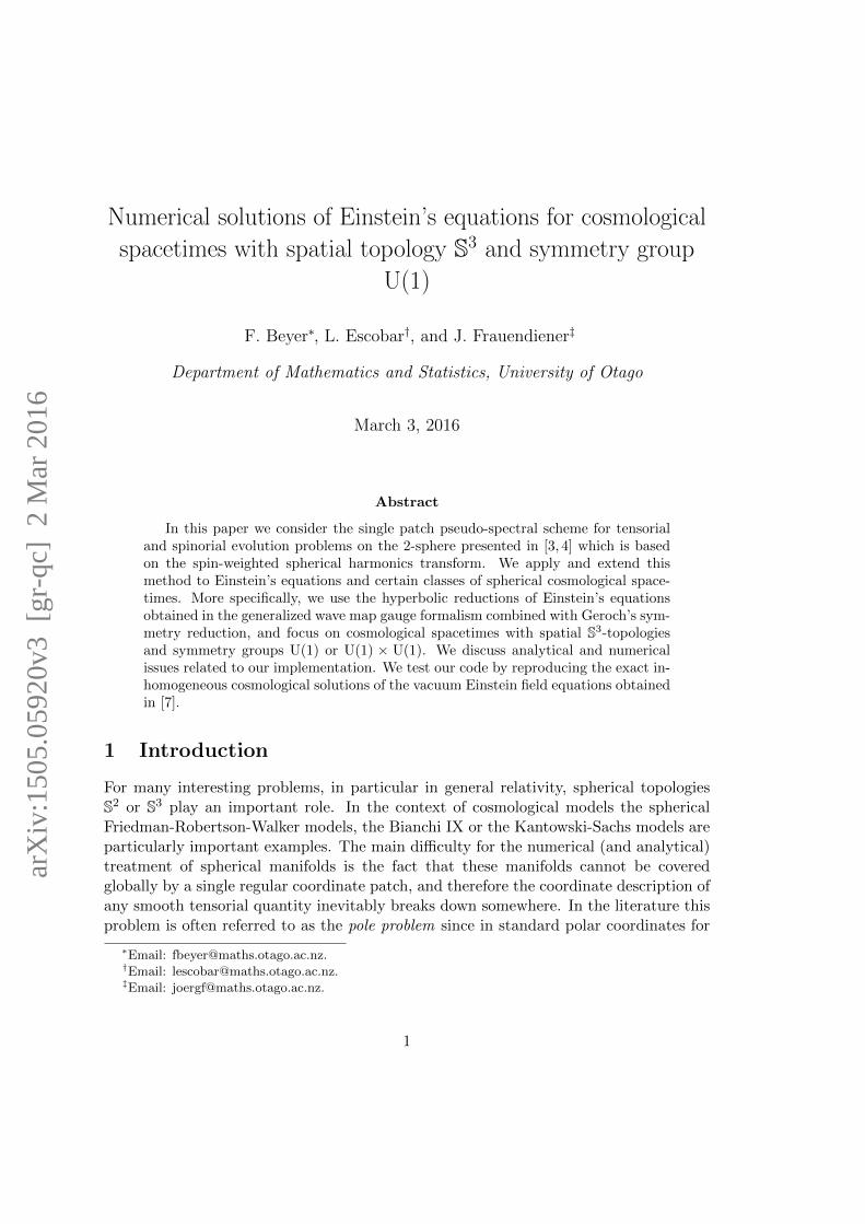
Let us consider a square integrable axially symmetric spin-weighted function f(ϑ) ∈L2(S2) with spin-weight s. Due to the ϕ dependence of the non-zero m modes of SWSH,see Eq. (4.1), we can write the function f(ϑ) in terms of only sYl0(ϑ, ϕ). Hence, theforward spin-weighted spherical harmonic transform Eq. (4.1) can be written in a simpleform as

sal =

∫S2

f(ϑ) sY l(ϑ) sinϑ dϑ dϕ,

where we have used the notation sal = sal0 and sYl(ϑ) = sYl0(ϑ, ϕ). Then, we rewriteEq. (4.4) as

sal = is√

2l + 1

4π

l∑n=−l

∆ln0In∆l

ns, (4.6)

with2

In := 2π

π∫0

e−inϑ f(ϑ) sinϑ dϑ. (4.7)

Similarly to what is done for HWTs in [29], the number of computations required toobtain the spectral coefficients sal can be reduced by a factor of 2 by using symmetriesassociated with the ∆l

mn quantities. In addition, we can introduce another reduction duethe fact that ∆l

n0 = 0 for l+n = odd. This allows to reduce the number of computationsby a further factor of 2. Therefore, we define the axially symmetric spin-weighted forwardtransform (ASFT) as

sal = is√

2l + 1

4π

l∑n=l(mod2)

∆ln0Jn∆l

ns (n+= 2), (4.8)

where n is a positive integer that increases in steps of two and starts at 0 or 1 dependingon whether l is even or odd. The vector Jn is defined by

Jn :=

In n = 0,

In + (−1)sI(−n) n > 0.(4.9)

2The factor 2π comes from the trivial integral over ϕ.

13

Figure 1

The evaluation of In can be carried out by extending the function f(ϑ) to T = S1 as a 2π-periodic function. This allows the implementation of the standard 1-dimensional Fouriertransform in contrast to the general case of HWTs which, due to the ϕ dependence,requires a 2-dimensional Fourier transform. Now, let us define the extended function onT as

sF (ϑ) :=

f(ϑ) ϑ ≤ π,(−1)s f(2π − ϑ) ϑ > π.

(4.10)

Clearly, the vector In remains unchanged because sF (ϑ) agrees with f(ϑ) on the integra-tion domain in Eq. (4.7). The function sF (ϑ) is chosen to be 2π periodic, hence it can bewritten as a 1-dimensional Fourier sum. However, before doing so we need to define thenumber of sampling points in T. Let us consider Fig. 1. In this diagram, the upper partof the circumference represents the number of samples Nϑ taken for 0 ≤ ϑ ≤ π, whereasthe lower part shows the Nϑ − 2 samples for π < ϑ < 2π. Clearly, the subtraction by2 in the lower half of the circumference comes from the extraction of the poles to avoidoversampling. Therefore, to sample a function on T we proceed as follows. If the desirednumber of samples for a function f(ϑ) on S2 is Nϑ, then the number of samples forthe extended function sF (ϑ) on T should be N ′ϑ = 2(Nϑ − 1) and the spatial samplinginterval will be ∆ϑ = 2π/N ′ϑ. Therefore, the extended function can be written as a1-dimensional Fourier sum by

sF (ϑ) =

N ′ϑ/2∑k=−N ′ϑ/2+1

Fkeikϑ.

The substitution of this equation into Eq. (4.7) yields

In = 2π

N ′ϑ/2∑k=−N ′ϑ/2+1

Fkw(k − n), (4.11)

where w(p) is a function Z→ R defined by

w(p) =

π∫0

eipϑ sinϑ dϑ =

2/(1− p2) p even,

0 p odd, p 6= ±1,

±iπ/2 p = ±1.

14

By comparison with Eq. (4.11) we note that the latter is proportional to a discreteconvolution in the spectral space. Therefore, it can be evaluated as a multiplication inthe real space such that In is the 1-dimensional forward Fourier transform of 2π sF wras follows

In =2π

N ′ϑ

N ′ϑ−1∑q′=0

exp (−inq∆ϑ) sF (q′∆ϑ) wr(q′∆ϑ

),

where wr(q′∆ϑ) is the real-valued quadrature weight in T given by

wr(q′∆ϑ) =

N ′ϑ/2∑p=−N ′ϑ/2+1

e−ipq′∆ϑ w(p).

Finally, we want to emphasize that even though this way of sampling functions on Tallows to include the value of the extended function at the poles, it yields an evennumber of modes in spectral space. Hence, we will not have the same number of pos-itive and negative modes after application of ASFT. Indeed, for the mode IN ′ϑ/2 (seeEq. (4.9)), the vector JL′ cannot be calculated since the term I−N ′ϑ/2 is not given by the1-dimensional forward Fourier. We avoid this issue by calculating the set of Jn terms upto n = N ′ϑ/2− 1. Note that setting IN ′ϑ/2 to zero does not constitute a loss of informa-tion due to the exponential decay of the spectral coefficients of the Fourier transform.In fact, this extra mode is in general numerically negligible and hence, it will not affectthe accuracy of the ASFT.

Now, in order to satisfy the Nyquist condition [17], the relation between the numberof sampling points in T and the band limit must satisfy the inequality

2(Nϑ − 1) ≥ (2L+ 1) + 1,

where the last term on the right-hand side comes from counting the extra term withoutmirrored partner. As a result, the maximum value of the band limit for which the ASFTis exact is

L = Nϑ − 2. (4.12)

4.2.2 The axially symmetric spin-weighted backward transform

This transform maps the spectral coefficients sal back to the corresponding axially sym-metric function on S2. As the inverse transform does not contain integrals, issues ofquadrature accuracy do not arise. In a similar way as we implemented the properties ofthe 3-dimensional ∆l

nm term to obtain Eq. (4.8), we can write from Eq. (4.5) the axiallysymmetric spin-weighted backward transform (ASBT) as

f(ϑ) =

N ′ϑ/2∑n=−N ′ϑ/2+1

einϑGn,

15

where the vector Gn is given by

Gn :=

0 if n = N ′ϑ/2,

isL∑

l≡mod2(n)

√2l+14π ∆l

n(−s) sal ∆ln0 (l+= 2).

(4.13)

Similar to Eq. (4.8), l increases in steps of two and starts at l(mod2). We set GN ′ϑ/2 = 0because in the implementation of the ASFT we chose IN ′ϑ/2 = 0. The evaluation ofEq. (4.13) is carried out by a 1-dimensional inverse Fourier transform that results ina function sF (ϑ) sampled on T. This function satisfies the symmetry properties inEq. (4.10) where f(ϑ) represents the function sF (ϑ) on 0 ≤ ϑ ≤ π. Thus, sF (ϑ)corresponds to the extension of the function f(ϑ) on T.

4.2.3 Computation of the 3-dimensional ∆lnm

So far the forward and backward spin-weighted spherical harmonic transforms have beensimplified for axially symmetric functions by the implementation of a 1-dimensionalFourier transform instead of a 2-dimensional one as required in the algorithm HWT.In fact, we can simplify the computation of the ∆l

nm terms even further. This has asignificant effect on the efficiency of both ASFT and ASBT, given that such a task takesaround half of the execution time in practical situations. We therefore devote this sectionto discuss this issue.

Before we explain how the ∆lnm terms are computed, we bring up a relevant fact for

both ASFT and ASBT. By examination of Eq. (4.8) and Eq. (4.13), we realize that we donot really need to calculate the complete set of ∆l

nm terms3 to perform the transform.Instead, we just need to compute up to the ∆l

ns term, where s is the spin-weight ofthe function that is supposed to be transformed. This yields a remarkable speed-up ofthe algorithm since in most cases s L. Now, based on this, we proceed to computethe ∆l

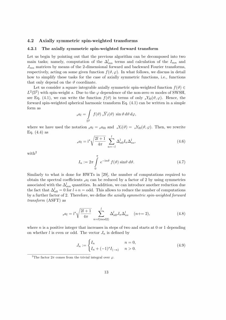
ns terms implementing the recursive algorithm introduced by Trapani and Navazain [45]. The recursive relations are given by the following equations

(a) ∆ll0 =

√2l − 1

2l∆l−1

(l−1)0,

(b) ∆llm =

√l(2l − 1)

2(l +m)(l +m− 1)∆l−1

(l−1)(m−1),

(c) ∆lnm =

2m√(l − n)(l + n+ 1)

∆l(n+1)(m) −

√(l − n− 1)(l + n+ 2)

(l − n)(l + n+ 1)∆l

(n+2)(m),

where the letters “(a)”, “(b)” and “(c)” denote the sequence in which they should beused. We note that terms with a combination of indices outside of the correct rangeare set to 0. One way to visualize the above algorithm is by means of the pyramidalrepresentation of the ∆l

ns terms in Fig. 2. The volume of the complete pyramid represents

3 n and m take integer values from −l to l.

16

Figure 2 Figure 3

the complete set of the ∆lnm terms. Setting the top peak of the pyramid as ∆0

00 = 1,we start moving down both in the vertical direction using rule (a), and in the diagonaldirection by (b). Thus, one can find the ∆l

ns terms in the right-hand side in the frontface of the pyramid. Then, using rule (c) repeatedly, one can find the terms behindthe front face in order to calculate the right-hand side of the pyramid volume. If weneed to compute the full set of ∆l

nm terms, we would need to repeat this algorithm inorder to obtain the complete right-hand side of the pyramid volume. However, we justneed to repeat step (b) until we reach the row corresponding to l = |s| (for the givenl-level) because we are just interested in computing the first ∆l

ns terms. Moreover, sinceonly the ∆l

ns terms with positive values of n are needed to compute both ASFT andASBT (see Eqs. (4.8) and (4.13)), we apply rule (c) until we reach the column n = 0.The left-hand side of the pyramid volume can be obtained by applying the mirror rule∆ln(−|s|) = (−1)l−n∆l

n|s| (see [45]). In Fig. 3, we display a schematic representation

of this, where the number of ∆lns terms that have to be computed are represented by

the gray section. In this illustration we consider the collection of the ∆lns terms for

each l-plane. Note that the gray section is not a rectangle since we can implement thesymmetric transposition rule ∆l

n|s| = (−1)|s|−n∆l|s|n. In short, we will require O(L2)

operations to compute the ∆lns terms needed for implementing both ASFT and ASBT,

which will allow us to pre-compute the ∆lnm terms for a low memory cost in comparison

with the general algorithm for HWTs4.In conclusion, we have presented both the forward and backward spin-weighted spher-

ical harmonic transform for the axi-symmetric case by implementing simplifications ofthe general algorithm HWTs in order to optimize them for axially symmetric functionsin S2. The first main simplification is the replacement of the 2-dimensional by a 1-dimensional Fourier transform for both the forward and backward transforms. Thisreduces the number of computations to O(L log2 L). The second simplification lies inthe fact that both the forward and backward transforms do not need the full set of ∆l

nm

4For L = 1024, the memory cost of AST is v 1MB whereas for HWT is v 1GB.

17

terms in the axial case. Therefore, the resulting algorithm requires O(L2) operationsfor each transform. However, if we precompute the Wigner coefficients ∆l

mn then thetransform is only requires O(L log2 L) operations.

These transform have been implemented in a Python 2.7 module5. Furthermore,the module allows to define objects that represent spin weighted functions for which analgebra can be defined. Hence, it can be seen not only as a set of functions, but as aPython environment for working with axi-symmetric SWSH.

4.3 Choosing the optimal grid size

Because the axially symmetric transforms are based on the Fourier transform, we ex-pect that spectral coefficients decay exponentially to zero when the band limit tends toinfinity. Theoretically speaking, a function is described in spectral space by an infinitenumber of spectral coefficients. On the other hand, because of the machine roundingerror6, any sufficiently smooth function is described by a finite set of spectral coefficientsthat contribute numerically to the spectral decomposition. In other words, the spectralcoefficients with order lower than 10−15 are negligible numerically, and thus are not nec-essary for an accurate description of functions in the spectral space. Hereafter, we callthe l-order of the last mode above order 10−15 as the optimal band limit. Consequently,in virtue of Eq. (4.12) the optimal band limit defines the optimal number of grid points.Taking a larger number of grid points than the optimal one will add unnecessary compu-tations in the transform and consequently the accuracy is reduced instead of enhanced.We refer to this as the sampling error. In our implementation we control this error bykeeping the number of grid points as close as possible to the optimal case. To this end,we proceed as follows. Initially, we sample the initial data in a large grid. In our casewe have chosen Nθ = 1025. Then, we apply the ASFT to each function of the initialdata and identify the highest mode which is just above the threshold 10−15. In otherwords, we identify the optimal band limit for each function of the system. From allthese modes we set the order of the highest mode as the optimal band limit for theinitial data. Henceforth we will refer to this as the global optimal band limit. UsingEq. (4.12) we obtain the optimal number of grid points required to sample the functionsof the system. Finally, we begin the numerical solution of the system by interpolatingthe initial data in the optimal grid. Now, we discuss how we keep the optimal grid sizeduring the evolution. For each time step, we check the last mode of each field in orderto observe whether they are smaller than some given tolerance. For this implementationthis has been set to 10−14. Then, if some of those modes do not satisfy the mentionedcondition, it implies that the number of grid points is not enough for sampling someof the functions of the system. Therefore, we need to interpolate all the functions to abigger grid. We point out that the new grid should not differ too much from the previous

5This module can be freely downloaded under the GNU General Public License (GPL) at http:

//gravity.otago.ac.nz/wiki/uploads/People/Axial_Spin_Weight_Functions.zip6In this paper, the terms “machine rounding error” and “machine precision” refer to the finite pre-

cision by which numbers can be represented in a computer. We always assume that this precision is ofthe order 10−15 which corresponds to standard “double precision”.

18

one because, as we mentioned before, it could lead to too many unnecessary grid pointsand hence to larger errors. In this implementation, we decided to increase the grid byfour points each time this is required. Using this small increment, we expect to stayclose enough to the optimal grid and as a consequence keep a good accuracy.

To finalize this section we point out that due to non-linearities in our evolutionequations, some kind of filtering process is required in order to avoid the so-called aliasingeffect. For this we use the well known 2/3-rule. For details and justification of this rule,see [17] and references therein.

5 Numerical application

5.1 Smooth Gowdy symmetry generalized Taub-NUT solutions

It is well known that solutions of Einstein’s field equations are uniquely determined(up to isometries and questions of extendibility) by the Cauchy data on a Cauchy sur-face. However, there exist cases for which the uniquely determined maximal globallyhyperbolic development [13] of the data can be extended in several inequivalent ways.These extensions are not globally hyperbolic and hence there are Cauchy horizons whosetopology and smoothness may in general be complicated. Furthermore, there can existclosed causal curves in the extended regions which violate basic causality conditions. Awell known example of this sort of solutions is the Taub solution [44], which is a two-parametric family of spatially homogeneous cosmological models with spatial topologyS3. Extensions through the Cauchy horizons are known as Taub-NUT solutions [37].

As generalizations of the Taub(-NUT) solutions, we consider now the class of smoothGowdy-symmetric generalized Taub-NUT solutions introduced in [6] motivated by earlywork by Moncrief [33]. These are Gowdy-symmetric globally hyperbolic solutions ofEinstein’s vacuum field equation with zero cosmological constant and spatial topologyS3 which have a past Cauchy horizon with topology S3 ruled by closed generators. Tocover the maximal global hyperbolic developments, the class is written in terms of the“areal” time function t ∈ (0, π) [14] and the same Euler coordinates as in Section 2.2 forthe spatial part. In these coordinates the metrics take the form

g = eM (−dt2 + dθ2) +R0

(sin2 t eu(dρ1 +Qdρ2)2 + sin2 θ e−udρ2

2

), (5.1)

with a positive constant R0 and smooth functions u, Q and M that depend only on tand θ. A large class of such solutions of the Einstein vacuum equations were constructedin [6] as an application of the Fuchsian method [1].

5.2 A family of exact solutions

In a subsequent paper [7], the same authors introduced a three-parametric family ofexplicit smooth Gowdy-symmetric generalized Taub-NUT solutions as an applicationof soliton methods. For this family of exact solutions, the components of the metric

19

Eq. (5.1) are given by

eM =R0

64c31

(U2 + V 2

), eu =

R0

64c21

Ue−M

1 + y,

Q = x+c3

8

(1− x2

)(7 + 4y + y2 +

(1− y)V 2

4c21U

),

where

U = c23

(1− x2

)(1− y)3 + 4c2

1(1 + y), V = 4c1 (1− y) (1− c3x(2 + y)) ,

with x = cosϑ, y = cos t. Here c1 and c3 are real constants that, together with R0, defineparticular solutions. We point out that this family of solutions contains the spatiallyhomogeneous Taub solutions as the special case given by

c1 =1

l

(√l2 +m2 +m

), c3 = 0, R0 = 2l

√l2 +m2,

with free parameters l > 0 and m ∈ R. Inhomogeneous solutions are obtained bychoosing any non-zero value for c3 (see [7] for details).

In the following we now perform the Geroch reduction described in Sections 2.1 and2.2 for these exact solutions. As a consequence of Gowdy symmetry, the vector field ∂ϕ isa smooth Killing field of the 2+1 metric hab. Consequently, all the metric components ofany Gowdy symmetric metric represented in these two coordinates are axial symmetricin the sense defined in Section 4 and hence the axial symmetric transform introducedin Section 4.2 is the natural choice for our numerical implementation discussed below.Before we discuss this in detail, we list the resulting formulas

ψ = R0 sin2 t eu, (5.2)

∂tω = −R0sin3 t

sinϑe2u∂ϑQ, (5.3)

∂ϑω = −R0sin3 t

sinϑe2u∂tQ, (5.4)

h = ψ(eM (−dt2 + dϑ2) +R0 sin2 ϑ e−udρ2

2

), (5.5)

where ψ and ω are the norm and twist associated with ∂ρ1 and hab the 2 + 1 metric.Next, as described in Section 3.2, we write the metric in terms of the frame (T,m,m)which yields

λ = R0 sin2 t eM+u, (5.6)

β = 0, (5.7)

δ = R0 sin2 t(eM+u +R0

)/2, (5.8)

φ = R0 sin2 t(eM+u −R0

)/2. (5.9)

Henceforth, we refer to hab as the 2+1 smooth Gowdy symmetry generalized Taub-NUTmetric.

20

We notice that the quantities Γµ associated with hab are calculated from Eq. (3.11)by first computing the contracted Christoffel symbols Γµ of hab and then by calculatingΓµ from Eq. (3.10) and the background metric Eq. (3.9). The results are

Γ0 = − cot t, (5.10)

Γ1 = Γ2 =√

2 c23 csc2 t sin8 t

2sin 2ϑ. (5.11)

Here, and in all of what follows, we choose c1 = 1, R0 = 2, and only vary c3.For the following it is also convenient to list the values of the metric functions at the

time t = π/2 which we shall use as the initial data for our numerical evolutions. Noticethat we cannot use t = 0 or t = π as initial times because the data are singular there.Thus, evaluating Eqs. (5.6)–(5.9) and time derivatives at t = π/2, we obtain7

λ0 = −4− c23 sin2 ϑ, ∂tλ0 = −4c2

3 sin2 ϑ, (5.12)

φ0 =c2

3

2sin2 ϑ, ∂tφ0 = c2

3 sin2 ϑ, (5.13)

δ0 = 4 +c2

3

2sin2 ϑ, ∂tδ0 = c2

3 sin2 ϑ, (5.14)

β0 = 0, ∂tβ0 = 0. (5.15)

From Eq. (5.2) and its time derivative we obtain the initial values for ψ0 and ∂tψ0

respectively. Finally, by integrating Eq. (5.4) with respect to ϑ and setting the irrelevantintegration constant to zero we obtain ω0. By considering Eq. (5.3) we obtain ∂tω0. Theexplicit form of these functions is

ω0 =−128(−8 + 16c3 cosϑ)

256 + 288c23 + 3c4

3 − 512c3 cosϑ− 4c23

(−56 + c2

3

)cos 2ϑ+ c4

3 cos 4ϑ,(5.16)

ψ0 =8(1 + 1

4c23 sin2 ϑ

)(1− 2c3 cosϑ)2 +

(1 + 1

4c23 sin2 ϑ

)2 , (5.17)

∂tω0 = 128(64 + 64c2

3 cos2 ϑ− 64c33 cos3 ϑ− 4c4

3 sin4 ϑ (5.18)

+c3 cosϑ(−128 + 8c2

3 sin2 ϑ+ 9c43 sin4 ϑ

) )/ B ,

∂tψ0 = −64c3

(128c3 cos2 ϑ− 32c3 sin2 ϑ+ 4c3

3 sin4 ϑ+ c53 sin6 ϑ (5.19)

+16 cosϑ(−12 + 5c2

3 sin2 ϑ)− 24c3

3 sin2 2ϑ)/ B ,

whereB =

(32− 64c3 cosϑ+ 64c2

3 cos2 ϑ+ 8c23 sin2 ϑ+ c4

3 sin4 ϑ)2.

5.3 Numerical error sources

The purpose of the following subsections is to describe the numerical evolution of theequations (3.13) for the just discussed initial data. We shall do this for two sets of gauge

7We have used ∂tg0 to denote the temporal partial derivative of any function g evaluated at the initialtime.

21

source functions. Before we go into the details in Sections 5.4 and 5.5, however, let usdiscuss possible numerical error sources which we shall refer to in our discussion of ournumerical results below.

Clearly the time and spatial discretization gives rise to numerical errors. In generalit is expected that time discretization errors are larger than spatial ones thanks to therapid (exponential) convergence of the latter. In order to investigate the presumablymore significant time discretization errors we shall use two different time discretizationschemes, the (non-adaptive) 4th-order Runge-Kutta scheme and the (adaptive) Runge-Kutta-Fehlberg (RKF) scheme. See [16] for details about adaptive Runge-Kutta meth-ods. Spatial discretizations shall always be based on our adaptive framework discussedin Section 4.3. For runs using the adaptive RKF scheme, we can therefore expect thatall discretization errors can be made sufficiently small by choosing suitable toleranceparameters.

In our numerical experiments we identify further error sources which turn out to beparticularly severe. Recall from Section 4.3 that we choose the same band limit for allunknowns. However, in most of our practical examples, only few of the unknowns actu-ally require high spatial resolutions. As a consequence, many unknowns are oversampled,which is not only inefficient numerically, but also generates undesired numerical noise.The origin of this noise is that the “unnecessary” modes associated with too large bandlimits are in general not zero numerically. In fact, while they are typically of the orderof the machine precision initially, they may grow during the evolution in particular duenonlinear coupling of modes. Typically, the larger the difference between the optimalband limit for any particular unknown and the global band limit is, the larger is thisnoise. This error is difficult to control in practice and it is quite common that once thisnoise has started to grow during the evolution it continues to grow increasingly fast. Wemeasure this error by looking at the evolution of the highest modes of certain represen-tative unknowns during the evolution. The only conceivable cure of this problem wouldbe to work with higher machine precisions, which would, however, significantly slowdown the numerical runs. Our numerical infrastructure is completely based on “dou-ble precision”. We have not attempted to work with higher machine precisions such as“quad precision” yet. Further comments on this in the context of a different numericalinfrastructure can be found, for example, in [2].

Another severe, but not fully independent numerical error is associated with theviolation of the constraints. Recall that due to Eq. (3.4), the condition Dµ ≡ 0 is iden-tically satisfied during the evolution if (i) the evolution equations hold exactly and (ii)the constraints Eqs. (3.5) and (3.6) are satisfied initially. For our numerical calculations,however, both of these conditions are violated. Let us for the sake of this argument imag-ine that the constraints are violated at the initial time, but that the evolution equationshold identically (i.e., we pretend that the numerical evolutions are done with an infiniteresolution in space and time and with infinite machine precision). Then Eq. (3.4) de-scribes the (exact) evolution of the in general non-zero constraint violation quantitiesDµ. Since the initial data for these quantities are now assumed to be non-zero, theirevolution is in general also non-zero. Depending on the particular properties of the evo-

22

lution system and hence of Eq. (3.4), these quantities may in fact grow rapidly duringthe evolution. If this is the case, the constraint violation error can become large veryquickly even if it is small at the initial time, and the resulting numerical solutions of Ein-stein’s equations therefore become useless quickly. This situation cannot be improved byincreasing the numerical resolution. In fact, this error is a consequence of the structureof the continuum evolution equations. Various ways to reconcile this problem have beenproposed in the literature. One of the most promising ideas [5, 9, 26] is to introduceconstraint damping terms, i.e., to add terms to the evolution equations (i) which areproportional to the constraint violation quantities (hence the solutions of the evolutionequations for the actual case of interest Dµ ≡ 0 are unchanged) and (ii) which, however,turn the surface Dµ ≡ 0 into a future attractor for Eq. (3.4). This technique has provedto be quite useful to produce stable calculations for asymptotically flat spacetimes (seefor instance [8,28,31,38]). The analytic derivation of suitable constraint damping termsis in general difficult and is usually done based on approximations which may only holdin certain regimes of the evolution (see e.g., [20]). In this paper here we work withoutconstraint damping terms. Nevertheless, we remark that thanks to the close relationshipof our formulation of Einstein’s equations with the ones used in the above references,similar choices of constraint damping terms are expected to be useful in reducing theconstraint violation errors in our applications. Indeed we have already gathered somepromising experience with constraint damping terms of the type used in [38] which weshall report on in a future article.

5.4 Numerical evolutions in areal gauge

In this section now, we shall fix the gauge freedom for the evolution equations by iden-tifying the gauge source functions fµ with the contracted Christoffel symbols given byEqs. (5.10) – (5.11); we recall that we have implicitly always assumed Eq. (3.9) as thereference metric and continue to do so. As common in the literature, we refer to thiscoordinate gauge as areal gauge. We shall then evolve the evolution equations (3.13)for the initial data given by Eqs. (5.12) – (5.19) at t = π/2 using these gauge sourcefunctions. The resulting numerical solutions are given in the same coordinates as theexact solution and direct comparisons between the exact and the numerical solutionscan be performed conveniently by considering the error quantity

E(t) := maxµ,ν‖ h(e)

µν (t, ϑ)− h(n)µν (t, ϑ) ‖L2(S2) ,

where h(e)µν (t, ϑ) represents a frame component of the exact metric for any given t, whereas

h(n)µν (t, ϑ) represents the numerical value. The norm ‖·‖L2(S2) is approximated numerically

by the discrete `2-norm of the grid function vector. Notice that the same spacetimes inthe same coordinates have been constructed numerically with different methods in [27].However, in contrast to our discussion here, some of Einstein’s equations turn out to beformally singular in the “interior” of the Gowdy square in the formulation used thereand hence are ignored to avoid serious numerical problems.

23

0.5π 0.6π 0.7π 0.8π 0.9π πt

−30

−25

−20

−15

−10

Log

2[E

(t)]

∆t = 0.04

∆t = 0.02

∆t = 0.01

Figure 4: Convergence test, c3 = 0.2.

0 π/4 π/2 3π/4 πθ

0

1

2

3

4

5

6

ψ(θ

)

t = 1.581

t = 1.938

t = 2.3

t = 2.588

t = 2.793

t = 3.0

Figure 5: Norm of the Killing vector, c3 = 0.2.

0 π/4 π/2 3π/4 πθ

4

5

6

7

8

9

10

11

ω(θ

)

t = 1.581

t = 1.938

t = 2.3

t = 2.588

t = 2.793

t = 3.0

Figure 6: Twist of the Killing vector, c3 = 0.2.

As a first test for our numerical implementation we present a convergence test inFig. 4 for c3 = 0.2. The evolution is carried out with the (non-adaptive) 4th-orderRunge-Kutta scheme. The figure shows the expected convergence rate demonstratingthat the time discretization error is dominant here. This is not surprising since at eacht all the metric components are very smooth functions that can be resolved on the gridwith high accuracy so long as t does not get too close to t = π. The oversamplingand constraint violation errors discussed in the previous subsection are small during thisearly phase of the evolution.

Next, we replace the non-adaptive 4th-order Runge-Kutta scheme by the adaptiveRKF method. In Fig. 5 and Fig. 6 we show the numerical evolutions of the geometricquantities ψ and ω for c3 = 0.2. The numerical error in these calculations are shown inFig. 7 for different values of c3. The error tolerance Tol of the RKF method is chosen tobe 10−8. This figure suggests that the numerical errors here remain bounded for a longtime. The larger c3 is, however, and hence the more inhomogeneous the solution is, themore rapidly the numerical errors grow close to t = π as expected. Fig. 8 indicates that

24

0.5π 0.6π 0.7π 0.8π 0.9π πt

−10.0

−9.5

−9.0

−8.5

−8.0

Log

10[E

(t)]

c3 = 0.15

c3 = 0.2

c3 = 0.25

c3 = 0.3

Figure 7: Error propagation for various valuesof c3 and Tol = 10−8.

0.5π 0.6π 0.7π 0.8π 0.9π πt

−14

−13

−12

−11

−10

−9

−8

Log

10[E

(t)]

Tol = 10−8

Tol = 10−9

Tol = 10−10

Figure 8: Error propagation for various valuesof Tol and c3 = 0.3.

0.5π 0.6π 0.7π 0.8π 0.9π πt

−14

−13

−12

−11

−10

−9

−8

Log

10[D

(t)]

Tol = 10−8

Tol = 10−9

Tol = 10−10

Figure 9: Constraints propagation for various values of Tol and c3 = 0.3.

the behavior close to t = π cannot be improved by decreasing the value of Tol. Thissuggests that close to t = π the numerical errors are not dominated anymore by the timediscretization error, but that one of the other error sources discussed in Section 5.3 takesover. Our experience suggests that in fact both the oversampling error and the constraintviolation error are significant at late times, in particular, for larger values of c3. As aconsequence of Eqs. (5.12) – (5.19), the required band limits for the metric componentsand their time derivatives are small, but the required band limits to resolve ψ0, ω0 andtheir time derivatives are relatively large. This discrepancy, which we associate with theoversampling error, is in fact larger the larger c3 is. As already mentioned before, thenoise generated by oversampling indeed grows during the evolution.

In order to measure the constraint violation error, we define the quantity

D(t) := maxµ‖ fµ(t, ϑ)− Γµ(t, ϑ) ‖L2(S2).

In Fig. 9, we show the evolution of this quantity for c3 = 0.3. At late times, the curves

25

look very similar to the ones of E(t) in Fig. 8. This suggests that the constraint violationerror contributes significantly to the total numerical error.

5.5 Numerical evolutions in wave map gauge

In this section we describe numerical computations for the same spacetimes as before,but using a different coordinate gauge. To this end, we want to choose the same initialdata as before, but work with different gauge source functions. Both the gauge constraintEq. (3.5) and the physical constraints Eq. (3.6) clearly have to be satisfied at the initialtime. Since we do not want to resolve these complicated nonlinear PDEs, our strategyis to use exactly the same initial data for the values of the metric components and theirfirst time derivative values, and also exactly the same initial values of the gauge sourcefunctions as before. In order to implement a different coordinate gauge, we then applythe following “gauge driver condition” during the evolution whose purpose is to rapidlydrive the gauge source functions from their initial values fixed by the gauge constrainttowards the target gauge source functions fµ:

fµ = (Γµ|t0 − fµ)e−q(t−t0) + fµ. (5.20)

Here the parameter q controls how rapidly the gauge is driven towards the target. Thequantities Γµ|t0 are calculated from the initial data and are understood as functions ofthe spatial coordinates only. Notice that different gauge drivers for the generalized waverepresentation of Einstein’s equations were considered in [32]. Eq. (5.20) guarantees thatthe gauge constraint is satisfied at the initial time. As discussed at the end of Section 3.1,the physical constraints, even though they pose highly non-trivial restrictions on thechoice of the initial data because they are essentially linear combinations of the well-known Hamiltonian and momentum constraints, turn out to not be restrictions on thegauge source functions. Hence it is not necessary to introduce terms in Eq. (5.20) whichaccount for the first time derivative of Γµ at t = t0.

We apply this idea to calculate the same spacetimes as before, but now we choosethe wave gauge as the target gauge, which is defined by the condition fµ = 0. For ournumerical tests we choose q = 10 in Eq. (5.20). Before we present our numerical resultswe notice that it is straightforward to derive the formula

t(w) =π

2+

1

2log

(1− cos t

1 + cos t

), (5.21)

which for our spacetimes relates the time coordinate t in areal gauge (used in Section 5.4)and the time coordinate t(w) in wave map gauge. This formula holds identically eventhough Eq. (5.20) is strictly speaking not the exact wave map gauge. However as aconsequence of Γ0|t0=π/2 = 0 which follows from Eq. (5.10), the target gauge source

function f0 = 0 agrees identically with f0 = 0. Eq. (5.21) is then obtained by solvingthe exactly homogeneous wave map equation for the wave map time coordinate functionwith appropriate initial conditions. Eq. (5.21) allows us to make direct comparisonsbetween our results here and the results in the previous section. In particular, it reveals

26

that the wave time slices t(w) = const are the same as the areal time slices t = const(for different constants), and, the “singularities” at t = 0, π are shifted to infinity, inparticular, t(w) → ∞ for t → π. We point out however that it is not possible to derivea formula which relates the spatial coordinates in both gauges. This is true even ifq in Eq. (5.20) was so large that we could consider our gauge as the exact wave mapgauge. This is a consequence of the fact that the homogeneity of the wave equations forthe spatial wave map coordinates is destroyed by terms given by the reference metricEq. (3.9). In fact we shall demonstrate below that the spatial coordinates on each timeslice are different in areal and wave map coordinates.

In order to obtain a more geometric and detailed comparison of the two gauges, weconsider the Eikonal equation following [19]

∇aτ∇aτ = −1. (5.22)

Let τ be a smooth solution of the initial value problem of the Eikonal equation withsmooth initial data τ0 : Σ0 → R prescribed freely on any smooth Cauchy surface Σ0

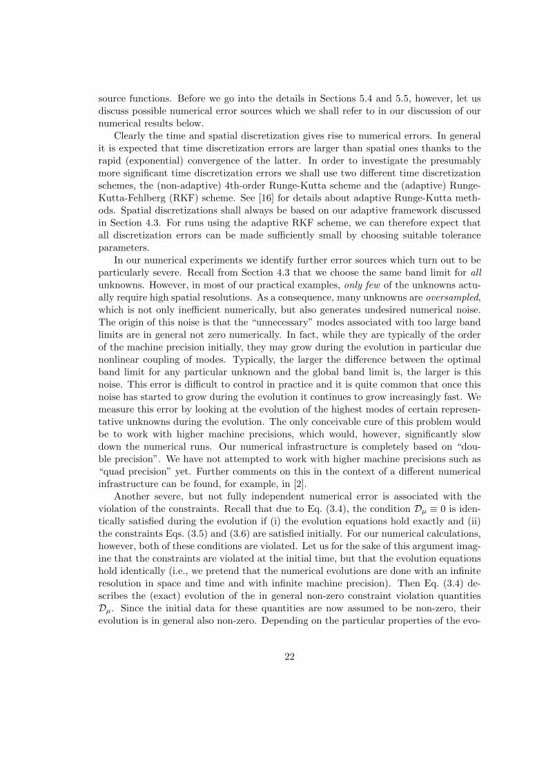
in any smooth globally hyperbolic spacetime. The method of characteristics applied tothis PDE allows to prove that such a solution indeed always exists at least sufficientlyclose to the initial hypersurface Σ0. For definiteness now we restrict to the case of zeroinitial data τ0 = 0 for all of what follows. Fix any point p in the timelike future ofΣ0 in the spacetime and consider any timelike geodesic through p (with unit tangentvector). Any such geodesic must intersect Σ0 at some point x0 in the past of p. There isprecisely one such timelike geodesic through p with unit tangent vector which intersectsΣ0 perpendicularly in x0 and hence the point x0 is uniquely determined. The valueτ(p) of the solution τ of the Eikonal equation with zero initial data then representsthe proper time along this timelike geodesic from x0 to p. The quantity τ is thereforea meaningful geometric scalar quantity which can be used to compare our numericalspacetimes, in particular when the same spacetime is calculated in different coordinategauges. We proceed as follows. For initial data parameters R0 = 2, c1 = 1 and c3 = 0.1(see Section 5.2):

1. We calculate the corresponding solution of Einstein’s evolution equations in arealgauge (in the same way as in Section 5.4) and of the Eikonal equation Eq. (5.22)(with zero initial data) up to t = 3. The value of the resulting τ function on thet = 3-surface expressed with respect to spatial areal coordinates yields the dashedcurve in Fig. 10.

2. Eq. (5.21) implies that t = 3 corresponds to t(w) ≈ 4.217. For the same initialdata parameters as in the first step, we calculate the corresponding solution ofEinstein’s evolution equations in wave gauge numerically (using the gauge drivercondition Eq. (5.20) with q = 10) and of the Eikonal equation Eq. (5.22) (withzero initial data) up to t(w) ≈ 4.217. The value of the resulting τ function on thet(w) ≈ 4.217-surface expressed with respect to spatial wave map coordinates yieldsthe continuous curve in Fig. 10.

27

0 π/4 π/2 3π/4 πΘ

1.98

1.99

2.00

2.01

2.02

2.03

2.04

2.05τ

Θ = θ Areal

Θ = θ(w)Wave

Figure 10: Proper time comparison.

0 π/4 π/2 3π/4 πθ

0.0000

0.0005

0.0010

0.0015

0.0020

diffe

renc

ebe

twee

nτ

func

tions

Figure 11: Difference of the proper times.

0.5π 0.75π πt

−8

−6

−4

−2

0

Log

10[D

(t)]

Areal

Wave

Figure 12: Comparison of the constraint violations.

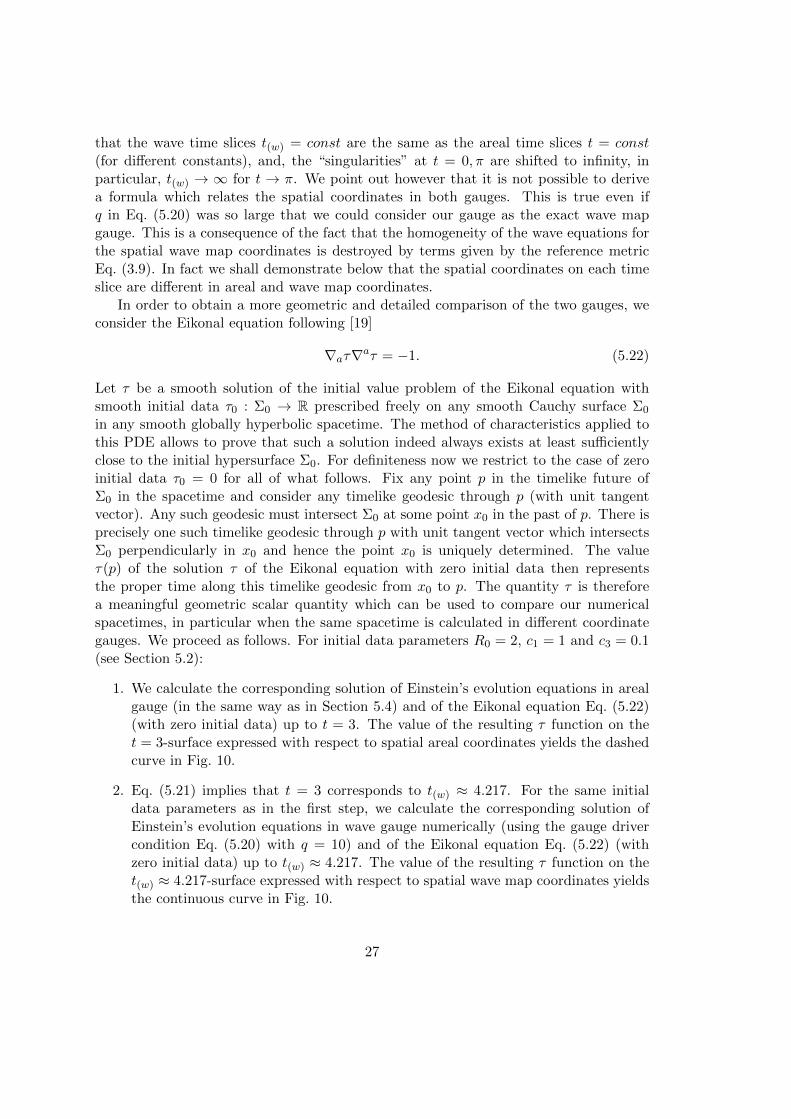
Since the t = 3-surface and the t(w) ≈ 4.217-surface represent the same geometric surfacein our spacetime and since τ is a geometric scalar quantity, the value of the solution ofthe Eikonal equation on this surface should be the same function in both steps above.However, since this function is expressed in terms of different spatial coordinates, namelyareal coordinates in the first step and wave map coordinates in the second step, thetwo curves in Fig. 10 are slightly different. Hence Fig. 10 can be understood as arepresentation of the difference of these two sets of spatial coordinates. This difference isemphasized in Fig. 11 where the two curves in Fig. 10 are subtracted directly. Intuitively,these two sets of spatial coordinates should agree at geometrically distinct points, namely,at the poles and also at the equator as a consequence of a reflection symmetry which isinherent to our particular class of exact solutions. Indeed the difference curve in Fig. 11is zero at the poles θ = 0, π and the equator θ = π/2.

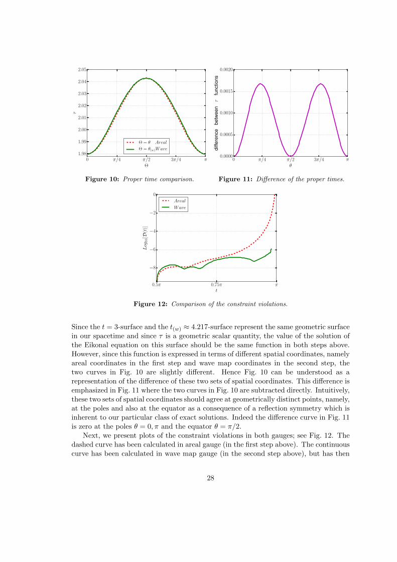
Next, we present plots of the constraint violations in both gauges; see Fig. 12. Thedashed curve has been calculated in areal gauge (in the first step above). The continuouscurve has been calculated in wave map gauge (in the second step above), but has then

28

been expressed in terms of the areal time function by means of Eq. (5.21). It is interestingto notice that the constraint violations are significantly smaller in wave map gauge thanthey are in areal gauge towards the end of the numerical evolution.

Finally we comment on the fact that in wave map gauge the shift quantity β inEq. (3.7) is a non-trivial non-zero function in contrast to areal gauge; see Eq. (5.7). Whenβ cannot be assumed to be zero identically, the algebraic complexity of the evolutionequations is increased dramatically. It is surprising that irrespective of this it appearsthat we get better numerical results in wave map than in areal gauge.

6 Discussion

The purpose of our work here was to introduce a numerical approach to solve the Cauchyproblem for spacetimes which involve the manifold S2. We employ a fully regular rep-resentation of the Einstein equations based on the spin-weighted spherical transformand the generalized wave map formalism. This allows us to account for all singularterms explicitly which usually arise as a consequence of the coordinate singularities ofpolar coordinates at the poles of the 2-sphere. Our numerical infrastructure is based onthe spin-weight formalism and corresponding transforms introduced in [3, 4]. We haveextended this infrastructure so that it now provides an efficient treatment of axially sym-metric functions on the 2-sphere, reducing the complexity O(L3) of the full transformto the complexity O(L2). We therefore expect this method to be useful also for otherapplications in future work. We have also demonstrated the consistency and feasibilityof our approach by means of numerical studies of certain inhomogeneous cosmologicalsolutions of the Einstein’s equations.

As another application of this method we are currently studying the critical behaviorof perturbations of the Nariai spacetime [3, 4]. In particular it is suggested that largeramplitudes of the perturbations, which had not been studied before, could lead to theformation of cosmological black holes. It would be of great interest to explore the thresh-old solutions and the expected cosmological black hole solutions as well as consequencesfor the longstanding cosmic no-hair and cosmic censorship conjectures. Other conceiv-able interesting applications where our numerical infrastructure can be applied directlyare Robinson-Trautman solutions [15] and Ricci flow [35].

A The generalized wave map formalism

Whether we want to solve the Cauchy problem for the 3 + 1-Einstein vacuum equationsGab + Λgab = 0 or for the 2 + 1 equations (2.4), the first task is always to extract hy-perbolic evolution equations and constraint equations with well-understood propagationproperties from the equation for the Ricci tensor of the unknown metric. We shall nowbriefly discuss the “generalized wave map formalism”. In most of the literature, therelated (but not covariant) generalized wave/harmonic formalism is used. While thisis sufficient for many applications, it is a drawback for us. In fact, for applicationswith spatial S2-topologies covered by a single singular polar coordinate system, it is far

29

more convenient to work with actual covariant quantities (i.e., smooth tensor fields).The reason is that frame components of smooth tensor fields on S2 have well-definedspin-weights (despite of the fact that the frame itself is singular at the poles) so thatthey are expandable in spin-weighted spherical harmonics, which are globally definedregular ‘functions’ on the 2-sphere (even though their coordinate representation may besingular). It turns out that expressing everything with respect to these bases, rendersthe equations manifestly regular.

To this end, we discuss the geometric formulation of the wave map gauge [21]. Weconsider a map Φ : M → M between two general smooth 4-dimensional manifolds Mand M (or open subsets thereof) equipped with Lorentzian metrics8 hab and hab. Themap Φ is called a wave map if it extremizes the functional

F [Φ] =

∫M

trh(Φ∗h) Volh.

In coordinate charts (xµ) on M and (yα) on M we obtain the Euler-Lagrange equationsfor the coordinate representation yα = yα(xµ) of Φ

hyα + Γαβγh

µν ∂yβ

∂xµ∂yγ

∂xν= 0. (A.1)

Here, Γαβγ are the Christoffel symbols for the metric hab in the coordinate basis onM , and h is the wave operator for scalar functions defined by hab. This equation iscalled the wave-map equation. More details can be found in [12]. If the manifolds wereRiemannian then the analogous equation would characterize a harmonic map between Mand M . Let us point out that the left hand side of the equation defines a geometric object,namely a section in the pull-back bundle Φ∗TM . This is not immediately obvious dueto the appearance of the Christoffel symbols in the second term. However, the tensorialcharacter of that term under change of coordinates in M is compensated for by the firstterm which, by itself, is also non-tensorial under such coordinate transformations.

The generalized wave-map equation is the equation (A.1) with a non-vanishing, ar-bitrary right hand side, a section in Φ∗TM with coordinate representation fα

hyα + Γαβγh

µν ∂yβ

∂xµ∂yγ

∂xν= −fα. (A.2)

The minus sign on the right-hand side is a matter of conventions. Suppose now thatM = M and Φ = idM . Then (xµ) and (yα) are two coordinate charts for M and (A.2)can be read as an equation determining the coordinate system (yα) for M by imposinga geometrical gauge condition. This equation is a semi-linear wave equation of M whichhas solutions near any Cauchy surface so that such a coordinate gauge always existslocally.

8All of the following arguments also hold if M and M are n-dimensional manifolds for some arbitrarypositive integer n and if hab is a general smooth pseudo-Riemannian (not necessary Lorentzian) metric.

30

Choosing the coordinates according to this gauge, i.e., putting xµ = yµ and express-ing the wave operator in these coordinates yields the equation

(−Γαβγ + Γαβγ)hβγ = −fα,

where Γαβγ are the Christoffel symbols of the metric h on M . In this equation thetensorial character becomes manifest since the left hand side involves the difference oftwo connection coefficients so it gives the components of a vector field in the coordinatebasis of the (xµ). Therefore, this equation holds in any basis on M as long as weinterpret the Christoffel symbols as the connection coefficients with respect to the chosenbasis. Note also that this implies that imposing the equation (A.2) does not constitutea condition on the coordinate system (xα) but a condition on the metric componentsin their dependence on the coordinates. We define the vector field Da in terms of itscomponents

Dα := (−Γαβγ + Γαβγ)hβγ + fα. (A.3)

So, Da = 0 when (A.2) is imposed. A metric hab which is restricted by Da = 0 is saidto be in wave map gauge (with respect to hab); in Eq. (3.9) we fix a particular metrichab. We point out that the wave map gauge reduces to the widely used generalizedwave/harmonic gauge characterized by xµ = −fµ on space-times with topology R4

when the Minkowski metric in Cartesian coordinates xµ is used as a reference metric hab.

References

[1] E. Ames, F. Beyer, J. Isenberg, and P. G. LeFloch. Quasilinear Hyperbolic FuchsianSystems and AVTD Behavior in T 2-Symmetric Vacuum Spacetimes. Ann. HenriPoincare, 14(6):1445–1523, 2013.

[2] F. Beyer. A spectral solver for evolution problems with spatial S3-topology. J.Comp. Phys., 228(17):6496–6513, 2009.

[3] F. Beyer, B. Daszuta, and J. Frauendiener. A spectral method for half-integerspin fields based on spin-weighted spherical harmonics. Class. Quantum Grav.,32(17):175013, 2015.

[4] F. Beyer, B. Daszuta, J. Frauendiener, and B. Whale. Numerical evolutions offields on the 2-sphere using a spectral method based on spin-weighted sphericalharmonics. Class. Quantum Grav., 31(7):075019, 2014.

[5] F. Beyer and L. Escobar. Graceful exit from inflation for minimally coupled BianchiA scalar field models. Class. Quantum Grav., 30(19):195020, 2013.

[6] F. Beyer and J. Hennig. Smooth Gowdy-symmetric generalized Taub–NUT solu-tions. Class. Quantum Grav., 29(24):245017, 2012.

[7] F. Beyer and J. Hennig. An exact smooth Gowdy-symmetric generalized Taub–NUTsolution. Class. Quantum Grav., 31(9):095010, 2014.

31

[8] M. Boyle, L. Lindblom, H. P. Pfeiffer, M. A. Scheel, and L. E. Kidder. Testing theaccuracy and stability of spectral methods in numerical relativity. Phys. Rev. D,75(2):024006, 2007.

[9] O. Brodbeck, S. Frittelli, P. Hubner, and O. A. Reula. Einstein’s equations withasymptotically stable constraint propagation. J. Math. Phys., 40(2):909, 1999.

[10] B. Brugmann. A pseudospectral matrix method for time-dependent tensor fields ona spherical shell. J. Comp. Phys., 235:216–240, 2013.

[11] M. W. Choptuik, E. W. Hirschmann, S. L. Liebling, and F. Pretorius. An axisym-metric gravitational collapse code. Class. Quantum Grav., 20(9):1857, 2003.

[12] Y. Choquet-Bruhat. General Relativity and the Einstein Equations. Oxford math-ematical monographs. Oxford University Press, Oxford, New York, 2008.

[13] Y. Choquet-Bruhat and R. P. Geroch. Global aspects of the Cauchy problem ingeneral relativity. Commun. Math. Phys., 14(4):329–335, 1969.

[14] P. T. Chrusciel. On space-times with U(1) × U(1) symmetric compact Cauchysurfaces. Ann. Phys., 202(1):100–150, 1990.

[15] H. P. de Oliveira, E. L. Rodrigues, and J. E. F. Skea. Numerical evolution of generalRobinson-Trautman spacetimes: Code tests, wave forms, and the efficiency of thegravitational wave extraction. Phys. Rev. D, 84(4):044007, 2011.

[16] D. R. Durran. Numerical Methods for Fluid Dynamics, volume 32 of Texts inApplied Mathematics. Springer, New York, NY, 2010.

[17] B. Fornberg. A Practical Guide to Pseudospectral Methods. Cambridge UniversityPress, 1998.

[18] Y. Foures-Bruhat. Theoreme d’existence pour certains systemes d’equations auxderivees partielles non lineaires. Acta Mathematica, 88(1):141–225, 1952.

[19] J. Frauendiener. Numerical treatment of the hyperboloidal initial value problemfor the vacuum Einstein equations. II. The evolution equations. Phys. Rev. D,58(6):064003, 1998.

[20] J. Frauendiener and T. Vogel. Algebraic stability analysis of constraint propagation.Class. Quantum Grav., 22(9):1769–1793, 2005.

[21] H. Friedrich. On the global existence and the asymptotic behavior of solutions tothe Einstein-Maxwell-Yang-Mills equations. J. Diff. Geom., 34:275–345, 1991.

[22] D. Garfinkle. Numerical simulations of Gowdy spacetimes on S2 × S1 × R. Phys.Rev. D, 60(10):104010, 1999.

32

[23] D. Garfinkle. Harmonic coordinate method for simulating generic singularities.Phys. Rev. D, 65(4):044029, 2002.

[24] R. P. Geroch. A Method for Generating Solutions of Einstein’s Equations. J. Math.Phys., 12(6):918, 1971.

[25] R. Gomez, L. Lehner, P. Papadopoulos, and J. Winicour. The eth formalism innumerical relativity. Class. Quantum Grav., 14(4):977–990, 1997.

[26] C. Gundlach, J. Martın-Garcıa, G. Calabrese, and I. Hinder. Constraint damping inthe Z4 formulation and harmonic gauge. Class. Quantum Grav., 22(17):3767–3774,2005.

[27] J. Hennig. Fully pseudospectral time evolution and its application to 1 + 1 dimen-sional physical problems. J. Comp. Phys., 235:322–333, 2013.

[28] M. Holst, L. Lindblom, R. Owen, H. P. Pfeiffer, M. A. Scheel, and L. E. Kid-der. Optimal constraint projection for hyperbolic evolution systems. Phys. Rev. D,70(8):084017, 2004.

[29] K. M. Huffenberger and B. D. Wandelt. Fast and Exact Spin-s Spherical HarmonicTransforms. Astro. J. Suppl. Series, 189(2):255–260, 2010.

[30] L. Lehner, O. A. Reula, and M. Tiglio. Multi-block simulations in general relativity:high-order discretizations, numerical stability and applications. Class. QuantumGrav., 22(24):5283–5321, 2005.

[31] L. Lindblom, M. A. Scheel, L. E. Kidder, H. P. Pfeiffer, D. Shoemaker, and S. A.Teukolsky. Controlling the growth of constraints in hyperbolic evolution systems.Phys. Rev. D, 69(12):124025, 2004.

[32] L. Lindblom and B. Szilagyi. Improved gauge driver for the generalized harmonicEinstein system. Phys. Rev. D, 80(8):084019, 2009.

[33] V. Moncrief. The space of (generalized) Taub-Nut spacetimes. J. Geom. Phys.,1(1):107–130, 1984.

[34] V. Moncrief. Reduction of Einstein’s equations for vacuum space-times with space-like U(1) isometry groups. Ann. Phys., 167(1):118–142, 1986.

[35] J. Morgan and T. Gang. Ricci Flow and the Poincare Conjecture. Clay MathematicsMonographs, 2007.

[36] E. T. Newman and R. Penrose. Note on the Bondi-Metzner-Sachs Group. J. Math.Phys., 7(5):863, 1966.

[37] E. T. Newman, L. Tamburino, and T. Unti. Empty-Space Generalization of theSchwarzschild Metric. J. Math. Phys., 4(7):915, 1963.

33

[38] F. Pretorius. Evolution of Binary Black-Hole Spacetimes. Phys. Rev. Lett.,95:121101, 2005.

[39] H. Ringstrom. The Cauchy Problem in General Relativity. ESI Lectures in Mathe-matics and Physics. European Mathematical Society, Zurich, Switzerland, 2009.

[40] O. Rinne. An axisymmetric evolution code for the Einstein equations on hyper-boloidal slices. Class. Quantum Grav., 27(3):035014, 2010.

[41] T. Risbo. Fourier transform summation of Legendre series and D-functions. J.Geodesy, 70(7):383–396, 1996.

[42] H. Stephani, D. Kramer, M. A. H. MacCallum, C. Hoenselaers, and E. Herlt. Exactsolutions of Einstein’s field equations. Cambridge University Press, second edition,2003.

[43] M. Sugiura. Unitary Representations and Harmonic Analysis. An Introduction.North Holland, 1990.

[44] A. H. Taub. Empty Space-Times Admitting a Three Parameter Group of Motions.Ann. Math., 53(3):472–490, 1951.

[45] S. Trapani and J. Navaza. Calculation of spherical harmonics and Wigner d-functions by FFT. Applications to fast rotational matching in molecular replacementand implementation into AMoRe. Acta Cryst. A, 62(4):262–269, 2006.

[46] A. Vretblad. Fourier Analysis and Its Applications. Springer New York, 2003.

34