arX

iva

stro

-ph

0005

004v

2 1

9 Ju

l 200

0

First Estimations of Cosmological Parameters from Boomerang

AE Lange1 PAR Ade2 JJ Bock3 JR Bond4 J Borrill5 A Boscaleri6 K Coble7 BP Crill1 P de

Bernardis8 P Farese7 P Ferreira9 10 K Ganga1 11 M Giacometti8 E Hivon1 VV Hristov1 A Iacoangeli8

AH Jaffe12 L Martinis13 S Masi8 PD Mauskopf14 A Melchiorri8 T Montroy7 CB Netterfield15 E Pascale6

F Piacentini8 D Pogosyan4 S Prunet4 S Rao16 G Romeo16 JE Ruhl7 F Scaramuzzi13 and D Sforna8

1California Institute of Technology Pasadena CA USA2Queen Mary and Westfield College London UK3Jet Propulsion Laboratory Pasadena CA USA

4Canadian Institute for Theoretical Astrophysics University of Toronto Canada5National Energy Research Scientific Computing Center LBNL Berkeley CA USA

6IROE-CNR Firenze Italy7Dept of Physics Univ of California Santa Barbara CA USA

8Dipartimento di Fisica Universitarsquo La Sapienza Roma Italy9Astrophysics University of Oxford NAPL Keble Road OX2 6HT UK

10Dept de Physique Theorique Universite de Geneve Switzerland11Physique Corpusculaire et Cosmologie College de France

11 place Marcelin Berthelot 75231 Paris Cedex 05 France12Center for Particle Astrophysics University of California BerkeleyCA USA13ENEA Centro Ricerche di Frascati Via E Fermi 45 00044 Frascati Italy

14Dept of Physics and Astronomy University of Massachussets Amherst MA USA15Depts of Physics and Astronomy University of Toronto Canada

16Istituto Nazionale di Geofisica Roma Italy

The anisotropy of the cosmic microwave background radiation contains information about thecontents and history of the universe We report new limits on cosmological parameters derived fromthe angular power spectrum measured in the first Antarctic flight of the Boomerang experimentWithin the framework of inflation-motivated adiabatic cold dark matter models and using onlyweakly restrictive prior probabilites on the age of the universe and the Hubble expansion parameterh we find that the curvature is consistent with flat and that the primordial fluctuation spectrumis consistent with scale invariant in agreement with the basic inflation paradigm We find thatthe data prefer a baryon density Ωbh

2 above though similar to the estimates from light elementabundances and big bang nucleosynthesis When combined with large scale structure observationsthe Boomerang data provide clear detections of both dark matter and dark energy contributionsto the total energy density Ωtot independent of data from high redshift supernovae

The angular power spectrum Cℓ of temperatureanisotropy in the cosmic microwave background (CMB)is a powerful probe of the content and nature of the uni-verse The DMR instrument on the COBE satellite mea-sured Cℓ for multipoles ℓ sim

lt 20 corresponding to angularscales simgt 7[1] Significant experimental effort by manygroups focusing on smaller angular scales when com-bined [2 3 4] led to the Cℓ estimates in the ℓ bandsmarked with xrsquos in Figure 1 which indicate a peak atℓ sim 200[5] It has long been recognized that if Cℓ can bedetermined with high precision over these angular scalesparameters such as the total energy density and baryoncontent of the universe and the shape of the primordialpower spectrum of density fluctuations can be accuratelymeasured [6] The most recently published Boomerang

angular power spectrum shown in Figure 1 representsa qualitative step towards such high precision [7] (here-after B98)

The data define a strong peak at ℓ sim 200 The steepdrop in power from ℓ sim 200 to ℓ sim 400 is consistent withthe structure expected from acoustic oscillations in adi-abatic cold dark matter (CDM) models of the universebut is not consistent with the locations and widths ofpeaks expected in the simplest cosmic string global topo-

logical defect and isocurvature perturbation models [8]The data at higher ℓ show strong detections which limitthe height of a second peak but are consistent with theheight expected in many CDM models

In this paper we concentrate on determining a setof 7 cosmological parameters that characterize a verybroad class of CDM models by statistically confrontingthe theoretical Cℓrsquos with the B98 and DMR data Sam-ple CDM models that fit the data are shown in Figure 1These are best-fit theoretical models using successivelymore restrictive ldquoprior probabilitiesrdquo on the parametersA major theme of this paper is to illustrate explicitlyhow inferences that are drawn from the CMB data de-pend on the priors that are assumed Some of these pri-ors are quite weakly restrictive and are generally agreedupon by most cosmologists for example that the Uni-verse is older than 10 Gyr and that the Hubble constantH0 = 100 h km sminus1Mpcminus1 lies between 45 and 90 Morestrongly restrictive priors rely on specific measurementseg the HST key project determination of H0 to 10accuracy [9] and the determination of the cosmologicalbaryon density ωb equiv Ωbh

2 to 10 [10]

In [7] we applied a ldquomediumrdquo set of priors to the B98power spectrum to constrain a 6 cosmological parame-

2

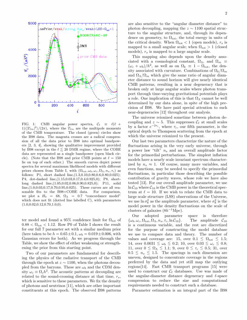
FIG 1 CMB angular power spectra Cℓ equiv ℓ(ℓ +1)〈|Tℓm|2〉(2π) where the Tℓm are the multipole momentsof the CMB temperature The closed (green) circles showthe B98 data The magenta crosses are a radical compres-sion of all the data prior to B98 into optimal bandpow-ers [2 3 4] showing the qualitative improvement providedby B98 except in the ℓ sim

lt 20 DMR regime where the COBEdata are represented as a single bandpower (open black cir-cle) (Note that the B98 and prior CMB points at ℓ = 150lie on top of each other) The smooth curves depict powerspectra for several maximum likelihood models with differentpriors chosen from Table I with (Ωtot ωb ωc ΩΛ ns τc) asfollows P1 short dashed line(13010080060800025)P4 dot-dashed line(1150030170409250) P8 short-long dashed line(10500200609008250) P11 solidline(100030170700950025) These curves are all rea-sonable fits to the B98+COBE data For comparisonwe plot a H0 = 68 ΩΛ = 07 ldquoconcordance modelrdquowhich does not fit (dotted line labelled C) with parameters(10002012070100)

ter model and found a 95 confidence limit for Ωtot of088 lt Ωtot lt 112 Row P0 of Table I shows the resultfor our full 7 parameter set with a similar medium prior(here taken to be h = 065plusmn01 ωb = 0019plusmn0006 withGaussian errors for both) As we progress through theTable we show the effect of either weakening or strength-ening the prior from this starting point

Two of our parameters are fundamental for describ-ing the physics of the radiative transport of the CMBthrough the epoch at z sim 1100 when the photons decou-pled from the baryons These are ωb and the CDM den-sity ωc equiv Ωch

2 The acoustic patterns at decoupling arerelated to the sound-crossing distance at that time rswhich is sensitive to these parameters We fix the densityof photons and neutrinos [11] which are other importantconstituents at this epoch The observed B98 patterns

are also sensitive to the ldquoangular diameter distancerdquo tophoton decoupling mapping the z sim 1100 spatial struc-ture to the angular structure and through its depen-dence on geometry to Ωtot the total energy in units ofthe critical density When Ωtot lt 1 (open models) rs ismapped to a small angular scale when Ωtot gt 1 (closedmodels) rs is mapped to a large angular scale

This mapping also depends upon the density asso-ciated with a cosmological constant ΩΛ and Ωm equiv(ωc + ωb)h2 as well as on Ωk equiv 1 minus Ωtot the den-sity associated with curvature Combinations of ΩkΩm

and ΩΛΩm which give the same ratio of angular diam-eter distance to sound horizon will give nearly identicalCMB patterns resulting in a near degeneracy that isbroken only at large angular scales where photon trans-port through time-varying gravitational potentials playsa role One implication of this is that ΩΛ cannot be welldetermined by our data alone in spite of the high pre-cision of B98 We have paid special attention to suchnear-degeneracies [12] throughout our analysis

The universe reionized sometime between photon de-coupling and z sim 5 This suppresses Cℓ at small scalesby a factor eminus2τc where τc our fifth parameter is theoptical depth to Thompson scattering from the epoch atwhich the universe reionized to the present

Our last two parameters characterize the nature of thefluctuations arising in the very early universe througha power law ldquotiltrdquo ns and an overall amplitude factorfor the primordial perturbations The simplest inflationmodels have a nearly scale invariant spectrum character-ized by ns asymp 1 Of course many more variables andeven functions may be needed to specify the primordialfluctuations in particular those describing the possiblecontribution of gravity waves whose role we have alsotested [13] For our overall amplitude parameter we useln C10 where C10 is the CMB power in the theoretical spec-trum at ℓ = 10 If we wish to relate the CMB data tolarge scale structure (LSS) observations of the Universewe use ln σ2

8 as the amplitude parameter where σ28 is the

model power in the density fluctuations on the scale ofclusters of galaxies (8hminus1Mpc)

Our adopted parameter space is thereforeωb ωc Ωtot ΩΛ ns τc ln C10 The amplitude C10

is a continuous variable and the rest are discretizedfor the purpose of constructing the model databasewe use to compare data and theory The number ofvalues and coverage are 15 over 01 minus

lt Ωtot minuslt 15

14 over 00031 minuslt ωb minuslt 02 10 over 003 minuslt ωc minuslt 0811 over 0 minus

lt ΩΛ minuslt 11 9 over 0 minus

lt τc minuslt 05 31 over

05 minuslt ns minuslt 15 The spacings in each dimension areuneven designed to concentrate coverage in the regionspreferred by the data and yet still map the outlyingregions[14] Fast CMB transport programs [15] wereused to construct our Cℓ databases Use was made ofthe angular-diameter distance degeneracy and ℓ-spacecompression to reduce the size and computationalrequirements needed to construct such a database

Parameter estimation is an integral part of the B98

3

analysis pipeline which makes statistically well-definedmaps and corresponding noise matrices from the time-ordered data from which we compute a set of maxi-mum likelihood bandpowers CB The likelihood curva-ture matrix FBBprime is calculated to provide error estimatesincluding correlations between bandpowers The curva-ture matrix FBBprime and the curvature matrix evaluatedat zero signal F0

BBprime are used in the offset-lognormal ap-proximation [2] to compute likelihood functions L(x ~y) =

P (~CB|x ~y) for each combination of parameters x and ~y inour database Here x is the value of the parameter we arelimiting ~y specifies the values of the other parameters

We multiply the likelihood by our chosen priors andmarginalize over the values of the other parameters ~yincluding the systematic uncertainties in the beamwidthand calibration of the measurement [16] This yields themarginalized likelihood distribution

L(x) equiv P (x|~CB) =

intPprior(x ~y)L(x ~y)d~y (1)

For clear detections central values and 1σ limits for theexplicit database parameters mentioned above are foundfrom the 16 50 and 84 integrals of L(x) Whenno clear detection exists these errors can be misleadingso for these cases we shift to likelihood falloffs by eminus12

from the maximum or variances about the mean of thedistribution L(x) The mean and variance are used toset the limits on other ldquoauxiliaryrdquo parameters such ash and Ωm which may be nonlinear combinations of thedatabase variables For good detections the three esti-mation methods give very good agreement and yield 2σerrors that are roughly twice the 1σ ones generally re-ported in this paper

We have used this method to estimate parameters us-ing the B98 power spectrum of Figure 1 with the COBEbandpowers determined by [2] and a variety of priorsThe results are summarized in Table I likelihood func-tions for selected parameters and priors are shown in Fig-ure 2

In the presence of degenerate and ill-constrained com-binations of parameters as with CMB data the edgesof the data-base form implicit priors We have con-structed our database such that these effective priors areextremely broad This allows us to probe the dependenceof our results on individually imposed priors The choiceof measure on the space is itself a prior we have used alinear measure in each of our variables [17] Sufficientlyrestrictive priors can break parameter degeneracies andresult in more stringent limits on the cosmological pa-rameters Artificially restrictive databases or priors canlead to misleading results thus priors should be bothwell motivated and tested for stability We therefore re-gard it as essential that the role of ldquohidden priorsrdquo in anychoice for Cℓ database construction be clearly articulated

To illustrate the effects of the database structure andapplied priors we have plotted likelihood functions foundusing only the database and priors (and no B98 data) inFigure 3 These should be compared with those plot-

ted in Figure 2 which include the B98 constraints asdiscussed below We now turn to the results found byapplying different priors in the general order of weakestto strongest applied priors

Our ldquoentire databaserdquo analysis prefers closed modelswith very high ωb as shown in line P1 of Table I and inFigure 2 The low sound speed of these models coupleswith the closed geometry to fit the peak near ℓ sim 200These models require very high values of h and ωb andhave extremely low ages so we have mapped out this re-gion using a coarse grid The dual-peaked projected like-lihood functions shown are reflections of the the complex-ity of the full 9-dimensional likelihood hypersurface Wenote that parameter combinations that appear to have alow probability based on the projected one-dimensionallimits can fit the data quite well eg the Ωtot = 1 best-fit model of Figure 1

Applying weakly restrictive priors (lines P2-P4 in Ta-ble I) moves the result away from the low sound speedmodels to a regime which is stable upon application ofmore restrictive priors as shown in panels 1 (top left)and 4 (bottom left) of Figure 2 Given their gross conflictwith many other cosmological tests we do not advocatethe ldquoentire databaserdquo models as representative of the ac-tual universe and we proceed with prior-limited analysesbelow

The analysis with weakly restrictive priors (P2-P4)finds that the curvature is consistent with flat whilefavoring slightly closed models The migration towardΩk = 0 as more restrictive priors are applied as shownin Table I and in panel 1 (top left) of Figure 2 suggestscaution in drawing any conclusion from the magnitude ofthe likelihood drop at Ωk = 0 In fact as is evident fromFigure 1 there are models with Ωk = 0 that fit the dataquite well The likelihood curve simply indicates thatthere are more models with Ωk lt 0 than with Ωk gt 0that fit the data well

We have taken special care to study the effect on thelikelihood distributions of choosing a different parame-terization of our database For example we have inves-tigated the likelihoods that result from a finely griddeddatabase that uses Ωc Ωb and h in place of Ωk ωband ωc to determine Ωk This second method restrictedto τc = 0 models uses these different variable choicesgridding and a completely different procedure and codewhich uses maximization of the likelihood over other vari-ables rather than marginalization To compare with thissecond method we have taken the database used for thetable and mimicked the effective priors due to the pa-rameter limits of the second database The results foundusing these two parameterizations and codes agree quitewell - in all cases the likelihood curves shift by at mosta small fraction of their width For example for the ap-plied priors of P2 the 95 confidence limits on Ωtot shiftfrom 099 lt Ωtot lt 124 for the method used in the tableto 094 lt Ωtot lt 127 for the Ωc Ωb and h method Dueto the very steep slope of the likelihood near Ωk = 0however even this small shift changes L(Ωk = 0)Lmax

4

from 02 to 08 We also find L(Ωk = 0)Lmax asymp 08if we use maximization rather than marginalization inthe code used for the table Additionally we note thata downward shift of about 5 in Ωtot occurs if the 10Gyr age constraint is removed from P2 These pointsplus the obvious compatibility of the data with the best-fit Ωtot = 1 curve in Fig 1 reinforces our conclusionthat there is no significant evidence in the B98 data fornon-zero curvature The only valid conclusion to drawfrom the data that we analyze in this paper is that thegeometry of the universe is very close to flat

The baryon density ωb is also well constrained Whileour results are higher (sim 3σ) than the ωb estimates fromlight element abundances [10] it is most remarkable thatour entirely independent method yields a result that is soclose to the BBN value The scalar spectral index ns isvery stable once weak priors are applied and is near thevalue expected from inflation This weak prior analysisdoes not yield a significant detection of ΩΛ the Ωch

2

results in Table I are suggestive of a detection but are atleast in part driven by the weak priors acting on limitsof the database [18 19] as shown in Figure 3 The valuesof τc are in the range of expectation of the models butthere is no clear detection

Note that the the weak priors adopt the conservativerestriction that the age of the universe exceeds 10 GyrWithout this the weak h prior still allows a contribu-tion albeit reduced from the high ωb low sound speedlow age solution With the age restriction this solutionis eliminated and the weak BBN prior (ωb minus

lt 05) doesnot significantly change the constraint thus the ldquoweakh+BBN+agerdquo (P4) and ldquoweak h+agerdquo (P2) rows are es-sentially identical

In row P4a we add a ldquoCMB priorrdquo which is a fulllikelihood analysis of all prior CMB experiments com-bined with B98 and DMR including appropriate fil-ter functions calibration uncertainties correlations andnoise estimates for use in the offset-lognormal approxi-mation [2] As would be expected given the errors wecompute on the compressed bandpowers of these experi-ments in Figure 1 cf those for B98 this CMB prior onlyslightly modifies the B98-derived parameters with ns themost notable migration None the less as much previ-ous analysis of the prior heterogeneous CMB datasetshas shown [20] reasonably strong cosmological conclu-sions could already be drawn on ns and Ωtot Row P4bshows results excluding B98 for the weak prior casethrough our machinery Though ns and Ωk have detec-tions consistent with the B98 results no conclusions canbe drawn on ωb (though the ldquowhole databaserdquo analysisdoes pick up the high ωb Ωtot region) We note that ifτc asymp 0 is enforced most variables remain unmoved butns which is well-correlated with τc moves closer to unityfor P4 P4a P4b we would have ns = 097 103 102respectively and for P5 P5a P5b we would have ns =093 098 098 A prior probability of τc based on ideas ofearly star formation would help to decrease the ns degreeof freedom

The Ωtot ωb and ns results are stable to the additionof a prior which imposes two constraints derived fromLSS observations [21] The first is an estimate of σ2

8

that requires the theory in question to reproduce the lo-cal abundance of clusters of galaxies The second is anestimate of a shape parameter for the density power spec-trum derived from observations of galaxy clustering [22]Adding LSS to the weak h and BBN priors (P5 and pan-els 2 (top center) and 3 (top right) of Figure 2) breaksa degeneracy yielding a detection of ΩΛ that is consis-tent with ldquocosmic concordancerdquo models This also occurswhen LSS is added to only the prior CMB data (P5band [21]) The LSS prior also strengthens the statisti-cal significance of the determination of Ωch

2 Panel 3(top right) of Figure 2 shows likelihood contours in theΩk equiv 1 minus Ωtot vs ΩΛ plane Here we have plotted theLSS prior (P5) which strongly localizes the contours [23]away from the ΩΛ = 0 axis toward a region that is highlyconsistent with the SN1a results [24] Indeed treatingthe SN1a likelihood as a prior does not change the re-sults very much as indicated by row P12 and P13 of theTable to be compared with rows P5 and P11 respec-tively

The use of a strong h prior alone yields results verysimilar to those for the weak h case The strong BBNprior however shifts many of the results from the weakBBN case Our data indicate a higher Ωbh

2 than BBNand constraining it with the BBN prior shifts the valuesof several parameters including Ωch

2 ΩΛ ns and ΩmAdditional ldquostrong priorrdquo results (P8-P11) are shown inTable I as an exercise in the power of combining otherconstraints with CMB data of this quality

A number of the cosmological parameters are highlycorrelated reflecting weak degeneracies in the broad butrestricted ℓ-space range that the B98+DMR data cov-ers [12] Some of these degeneracies can be broken withdata at higher ℓ as is visually evident in the radically dif-ferent behavior of the models of Figure 1 beyond ℓ sim 600To understand the degeneracies within the context of thisdata we have explored the structure of the parameter co-variance matrix 〈∆yi∆yj〉 both for the database param-eters and the ones derived from them They add motiva-tion for the specific parameter choices we have made [25]Parameter eigenmodes [6 12] of the covariance matrixfound by rotating into principal components explicitlyshow the combinations of physical database variablesthat give orthogonal error bars A by-product is a rank-ordered set of eigenvalues which show that for the cur-rent B98 data 3 combinations of the 7 parameters aredetermined to better than 10 [26]

We conclude that the B98 data are consistent with thepredictions of the basic inflationary paradigm that thecurvature of the universe is near zero (Ωk = 0) and thatthe primordial power spectrum is nearly scale-invariant(ns = 1) The slight preference that the current datashow for closed rather than open models is not webelieve a statistically significant indication of non-zerocurvature A more conclusive statement awaits further

5

analysis of B98 data which will increase the precision ofthe measured power spectrum andor the results fromother experiments

We measure a strong detection of the baryon densityΩbh

2 a first for determinations of this parameter fromCMB data The value that we measure is robust to thechoice of prior and is both remarkably close to and signif-icantly higher than that given by the observed light ele-ment abundances combined with BBN theory Assumingthat Ωtot = 1 we find Ωbh

2 = 0031 plusmn 0004Finally we find that combining the B98 data with our

relatively weak prior representing LSS observations andwith our other weak priors on the Hubble constant andthe age of the universe yields a clear detection of bothnon-baryonic matter (Ωch

2 = 0014+0003minus0002) and dark en-

ergy (ΩΛ = 066+007minus009) contributions to the total energy

density in the universe The amount of dark energy thatwe measure is robust to the inclusion of a prior on Ωtot

(shifting to ΩΛ = 067+004minus006 for Ωtot = 1) and to the

inclusion of the prior likelihood given by observationsof high-redshift SN1a (shifting to ΩΛ = 069+002

minus003 whenboth the Ωtot = 1 and the SN1a priors are included) The

perfect concordance between the completely independentdetections of ΩΛ from the CMB+LSS data and from theSN1a data is powerful support for the notion that theuniverse is currently dominated by precisely the amountof dark energy necessary to provide zero curvature

The analysis presented here and in [7] makes use ofonly a small fraction of the data obtained during the firstAntarctic flight of Boomerang Work now in progresswill increase the precision of the power spectrum fromℓ = 50 to 600 and extend the measurements to smallerangular scales allowing yet more precise determinationsof several of the cosmological parameters

AcknowledgementsThe Boomerang program has been supported by

NASA (NAG5-4081 amp NAG5-4455) the NSF Science ampTechnology Center for Particle Astrophysics (SA1477-22311NM under AST-9120005) and NSF Office of Po-lar Programs (OPP-9729121) in the USA ProgrammaNazionale Ricerche in Antartide Agenzia Spaziale Ital-iana and University of Rome La Sapienza in Italy and byPPARC in UK We thank Saurabh Jha and Peter Gar-navich for supplying the SN1a curves used in Figure 2

[1] C Bennett et al Astrophys J 464 L1 (1996)[2] J R Bond A H Jaffe and L Knox Astrophys J 533

19 (2000) The bandpowers used to construct the rad-ically compressed pre-Boomerang-LDB spectrum arelisted there except for the [3] and [4] data which we havealso included

[3] A D Miller et al Astrophys J 524 L1 (1999)[4] P Mauskopf et al Ap J Letters 536 L59 (2000)[5] L Knox and L Page submitted to Phys Rev Lett

astro-ph0002162 (2000)[6] eg J R Bond G Efstathiou and M Tegmark Mon

Not R Astron Soc 291 L33 (1997) and referencestherein see also [21] for forecasts of LDB parameter ex-traction performance

[7] P deBernardis et al Nature 404 955 (2000)[8] R Durrer A Gangui M Sakellariadou Phys Rev Lett

76 579-582 (1996) eg B Allen et al Phys Rev Lett79 2624 (1997) U Pen N Turok and U Seljak PhysRev D 58 023506 (1998) A Albrecht R A Battye andJ Robinson Phys Rev D 59 023508 (1999)

[9] W L Freedman astro-ph9909076 (1999) J R Mouldet al Astrophys J 529 786 (2000)

[10] K A Olive G Steigman and T P Walker submittedto Phys Rep astro-ph9905320 (1999) D Tytler J MOrsquoMeara N Suzuki and D Lubin submitted to PhysicaScripta astro-ph0001318 (2000)

[11] The Cℓ spectra with massive neutrinos are quite similarto those without and current data including B98 willnot be able to strongly constrain the value When theLSS prior is added to the CMB data however the com-bination is quite powerful eg [21]

[12] G Efstathiou and J R Bond Mon Not R Astron Soc304 75 (1999)

[13] Gravity waves (GW) can induce CMB anisotropy andcould have a separate tilt nt and an overall amplitude

They have little effect over the range of ℓrsquos that B98 ismost sensitive to but could have an important impacton the amplitude relative to COBE To test the role thatGW induced anisotropies would play we have adoptedthe model used by [21] for ns lt 1 we set nt = ns minus 1and for ns gt 1 we allow no GW contribution Thispresents a fixed alternative reasonably motivated by in-flation without introducing new parameters We havefound that there is a negligible effect on the parameterdeterminations in Table I there is only a very slight mi-gration upward in ns

[14] The specific values of the database variables used for thisanalysis are (ωc = 003 006 012 017 022 027 033040 055 08) (ωb = 0003125 000625 00125 001750020 0025 0030 0035 004 005 0075 010 01502) (ΩΛ =0 01 02 03 04 05 06 07 08 09 1011) (Ωk =09 07 05 03 02 015 01 005 0 -005-01 -015 -02 -03 -05) (ns =15 145 14 135 13125 12 1175 115 1125 11 1075 105 1025 100975 095 0925 09 0875 085 0825 08 0775 0750725 07 065 06 055 05) (τc =0 0025 005 007501 015 02 03 05)

[15] U Seljak and M Zaldarriaga Astrophys J 469437 (1996) httpwwwsnsiasedusimmatiaszCMB-FASTcmbfasthtml A Lewis A Challinor and ALasenby astro-ph9911177 (1999)

[16] Apart from the 7 stated database parameters we haveallowed for an estimated 10 uncertainty in the calibra-tion and the beam which we determine simultaneouslywith the overall amplitude C10 by relaxing to the maxi-mum likelihood value in these variables We then deter-mine the Fisher error matrix assume that the variablesare log-normally distributed and evaluate a correction tothe likelihoods appropriate for marginalization over theseldquointrinsicrdquo variables Including the marginalization cor-

3

analysis pipeline which makes statistically well-definedmaps and corresponding noise matrices from the time-ordered data from which we compute a set of maxi-mum likelihood bandpowers CB The likelihood curva-ture matrix FBBprime is calculated to provide error estimatesincluding correlations between bandpowers The curva-ture matrix FBBprime and the curvature matrix evaluatedat zero signal F0

BBprime are used in the offset-lognormal ap-proximation [2] to compute likelihood functions L(x ~y) =

P (~CB|x ~y) for each combination of parameters x and ~y inour database Here x is the value of the parameter we arelimiting ~y specifies the values of the other parameters

We multiply the likelihood by our chosen priors andmarginalize over the values of the other parameters ~yincluding the systematic uncertainties in the beamwidthand calibration of the measurement [16] This yields themarginalized likelihood distribution

L(x) equiv P (x|~CB) =

intPprior(x ~y)L(x ~y)d~y (1)

For clear detections central values and 1σ limits for theexplicit database parameters mentioned above are foundfrom the 16 50 and 84 integrals of L(x) Whenno clear detection exists these errors can be misleadingso for these cases we shift to likelihood falloffs by eminus12

from the maximum or variances about the mean of thedistribution L(x) The mean and variance are used toset the limits on other ldquoauxiliaryrdquo parameters such ash and Ωm which may be nonlinear combinations of thedatabase variables For good detections the three esti-mation methods give very good agreement and yield 2σerrors that are roughly twice the 1σ ones generally re-ported in this paper

We have used this method to estimate parameters us-ing the B98 power spectrum of Figure 1 with the COBEbandpowers determined by [2] and a variety of priorsThe results are summarized in Table I likelihood func-tions for selected parameters and priors are shown in Fig-ure 2

In the presence of degenerate and ill-constrained com-binations of parameters as with CMB data the edgesof the data-base form implicit priors We have con-structed our database such that these effective priors areextremely broad This allows us to probe the dependenceof our results on individually imposed priors The choiceof measure on the space is itself a prior we have used alinear measure in each of our variables [17] Sufficientlyrestrictive priors can break parameter degeneracies andresult in more stringent limits on the cosmological pa-rameters Artificially restrictive databases or priors canlead to misleading results thus priors should be bothwell motivated and tested for stability We therefore re-gard it as essential that the role of ldquohidden priorsrdquo in anychoice for Cℓ database construction be clearly articulated

To illustrate the effects of the database structure andapplied priors we have plotted likelihood functions foundusing only the database and priors (and no B98 data) inFigure 3 These should be compared with those plot-

ted in Figure 2 which include the B98 constraints asdiscussed below We now turn to the results found byapplying different priors in the general order of weakestto strongest applied priors

Our ldquoentire databaserdquo analysis prefers closed modelswith very high ωb as shown in line P1 of Table I and inFigure 2 The low sound speed of these models coupleswith the closed geometry to fit the peak near ℓ sim 200These models require very high values of h and ωb andhave extremely low ages so we have mapped out this re-gion using a coarse grid The dual-peaked projected like-lihood functions shown are reflections of the the complex-ity of the full 9-dimensional likelihood hypersurface Wenote that parameter combinations that appear to have alow probability based on the projected one-dimensionallimits can fit the data quite well eg the Ωtot = 1 best-fit model of Figure 1

Applying weakly restrictive priors (lines P2-P4 in Ta-ble I) moves the result away from the low sound speedmodels to a regime which is stable upon application ofmore restrictive priors as shown in panels 1 (top left)and 4 (bottom left) of Figure 2 Given their gross conflictwith many other cosmological tests we do not advocatethe ldquoentire databaserdquo models as representative of the ac-tual universe and we proceed with prior-limited analysesbelow

The analysis with weakly restrictive priors (P2-P4)finds that the curvature is consistent with flat whilefavoring slightly closed models The migration towardΩk = 0 as more restrictive priors are applied as shownin Table I and in panel 1 (top left) of Figure 2 suggestscaution in drawing any conclusion from the magnitude ofthe likelihood drop at Ωk = 0 In fact as is evident fromFigure 1 there are models with Ωk = 0 that fit the dataquite well The likelihood curve simply indicates thatthere are more models with Ωk lt 0 than with Ωk gt 0that fit the data well

We have taken special care to study the effect on thelikelihood distributions of choosing a different parame-terization of our database For example we have inves-tigated the likelihoods that result from a finely griddeddatabase that uses Ωc Ωb and h in place of Ωk ωband ωc to determine Ωk This second method restrictedto τc = 0 models uses these different variable choicesgridding and a completely different procedure and codewhich uses maximization of the likelihood over other vari-ables rather than marginalization To compare with thissecond method we have taken the database used for thetable and mimicked the effective priors due to the pa-rameter limits of the second database The results foundusing these two parameterizations and codes agree quitewell - in all cases the likelihood curves shift by at mosta small fraction of their width For example for the ap-plied priors of P2 the 95 confidence limits on Ωtot shiftfrom 099 lt Ωtot lt 124 for the method used in the tableto 094 lt Ωtot lt 127 for the Ωc Ωb and h method Dueto the very steep slope of the likelihood near Ωk = 0however even this small shift changes L(Ωk = 0)Lmax

4

from 02 to 08 We also find L(Ωk = 0)Lmax asymp 08if we use maximization rather than marginalization inthe code used for the table Additionally we note thata downward shift of about 5 in Ωtot occurs if the 10Gyr age constraint is removed from P2 These pointsplus the obvious compatibility of the data with the best-fit Ωtot = 1 curve in Fig 1 reinforces our conclusionthat there is no significant evidence in the B98 data fornon-zero curvature The only valid conclusion to drawfrom the data that we analyze in this paper is that thegeometry of the universe is very close to flat

The baryon density ωb is also well constrained Whileour results are higher (sim 3σ) than the ωb estimates fromlight element abundances [10] it is most remarkable thatour entirely independent method yields a result that is soclose to the BBN value The scalar spectral index ns isvery stable once weak priors are applied and is near thevalue expected from inflation This weak prior analysisdoes not yield a significant detection of ΩΛ the Ωch

2

results in Table I are suggestive of a detection but are atleast in part driven by the weak priors acting on limitsof the database [18 19] as shown in Figure 3 The valuesof τc are in the range of expectation of the models butthere is no clear detection

Note that the the weak priors adopt the conservativerestriction that the age of the universe exceeds 10 GyrWithout this the weak h prior still allows a contribu-tion albeit reduced from the high ωb low sound speedlow age solution With the age restriction this solutionis eliminated and the weak BBN prior (ωb minus

lt 05) doesnot significantly change the constraint thus the ldquoweakh+BBN+agerdquo (P4) and ldquoweak h+agerdquo (P2) rows are es-sentially identical

In row P4a we add a ldquoCMB priorrdquo which is a fulllikelihood analysis of all prior CMB experiments com-bined with B98 and DMR including appropriate fil-ter functions calibration uncertainties correlations andnoise estimates for use in the offset-lognormal approxi-mation [2] As would be expected given the errors wecompute on the compressed bandpowers of these experi-ments in Figure 1 cf those for B98 this CMB prior onlyslightly modifies the B98-derived parameters with ns themost notable migration None the less as much previ-ous analysis of the prior heterogeneous CMB datasetshas shown [20] reasonably strong cosmological conclu-sions could already be drawn on ns and Ωtot Row P4bshows results excluding B98 for the weak prior casethrough our machinery Though ns and Ωk have detec-tions consistent with the B98 results no conclusions canbe drawn on ωb (though the ldquowhole databaserdquo analysisdoes pick up the high ωb Ωtot region) We note that ifτc asymp 0 is enforced most variables remain unmoved butns which is well-correlated with τc moves closer to unityfor P4 P4a P4b we would have ns = 097 103 102respectively and for P5 P5a P5b we would have ns =093 098 098 A prior probability of τc based on ideas ofearly star formation would help to decrease the ns degreeof freedom

The Ωtot ωb and ns results are stable to the additionof a prior which imposes two constraints derived fromLSS observations [21] The first is an estimate of σ2

8

that requires the theory in question to reproduce the lo-cal abundance of clusters of galaxies The second is anestimate of a shape parameter for the density power spec-trum derived from observations of galaxy clustering [22]Adding LSS to the weak h and BBN priors (P5 and pan-els 2 (top center) and 3 (top right) of Figure 2) breaksa degeneracy yielding a detection of ΩΛ that is consis-tent with ldquocosmic concordancerdquo models This also occurswhen LSS is added to only the prior CMB data (P5band [21]) The LSS prior also strengthens the statisti-cal significance of the determination of Ωch

2 Panel 3(top right) of Figure 2 shows likelihood contours in theΩk equiv 1 minus Ωtot vs ΩΛ plane Here we have plotted theLSS prior (P5) which strongly localizes the contours [23]away from the ΩΛ = 0 axis toward a region that is highlyconsistent with the SN1a results [24] Indeed treatingthe SN1a likelihood as a prior does not change the re-sults very much as indicated by row P12 and P13 of theTable to be compared with rows P5 and P11 respec-tively

The use of a strong h prior alone yields results verysimilar to those for the weak h case The strong BBNprior however shifts many of the results from the weakBBN case Our data indicate a higher Ωbh

2 than BBNand constraining it with the BBN prior shifts the valuesof several parameters including Ωch

2 ΩΛ ns and ΩmAdditional ldquostrong priorrdquo results (P8-P11) are shown inTable I as an exercise in the power of combining otherconstraints with CMB data of this quality

A number of the cosmological parameters are highlycorrelated reflecting weak degeneracies in the broad butrestricted ℓ-space range that the B98+DMR data cov-ers [12] Some of these degeneracies can be broken withdata at higher ℓ as is visually evident in the radically dif-ferent behavior of the models of Figure 1 beyond ℓ sim 600To understand the degeneracies within the context of thisdata we have explored the structure of the parameter co-variance matrix 〈∆yi∆yj〉 both for the database param-eters and the ones derived from them They add motiva-tion for the specific parameter choices we have made [25]Parameter eigenmodes [6 12] of the covariance matrixfound by rotating into principal components explicitlyshow the combinations of physical database variablesthat give orthogonal error bars A by-product is a rank-ordered set of eigenvalues which show that for the cur-rent B98 data 3 combinations of the 7 parameters aredetermined to better than 10 [26]

We conclude that the B98 data are consistent with thepredictions of the basic inflationary paradigm that thecurvature of the universe is near zero (Ωk = 0) and thatthe primordial power spectrum is nearly scale-invariant(ns = 1) The slight preference that the current datashow for closed rather than open models is not webelieve a statistically significant indication of non-zerocurvature A more conclusive statement awaits further

5

analysis of B98 data which will increase the precision ofthe measured power spectrum andor the results fromother experiments

We measure a strong detection of the baryon densityΩbh

2 a first for determinations of this parameter fromCMB data The value that we measure is robust to thechoice of prior and is both remarkably close to and signif-icantly higher than that given by the observed light ele-ment abundances combined with BBN theory Assumingthat Ωtot = 1 we find Ωbh

2 = 0031 plusmn 0004Finally we find that combining the B98 data with our

relatively weak prior representing LSS observations andwith our other weak priors on the Hubble constant andthe age of the universe yields a clear detection of bothnon-baryonic matter (Ωch

2 = 0014+0003minus0002) and dark en-

ergy (ΩΛ = 066+007minus009) contributions to the total energy

density in the universe The amount of dark energy thatwe measure is robust to the inclusion of a prior on Ωtot

(shifting to ΩΛ = 067+004minus006 for Ωtot = 1) and to the

inclusion of the prior likelihood given by observationsof high-redshift SN1a (shifting to ΩΛ = 069+002

minus003 whenboth the Ωtot = 1 and the SN1a priors are included) The

perfect concordance between the completely independentdetections of ΩΛ from the CMB+LSS data and from theSN1a data is powerful support for the notion that theuniverse is currently dominated by precisely the amountof dark energy necessary to provide zero curvature

The analysis presented here and in [7] makes use ofonly a small fraction of the data obtained during the firstAntarctic flight of Boomerang Work now in progresswill increase the precision of the power spectrum fromℓ = 50 to 600 and extend the measurements to smallerangular scales allowing yet more precise determinationsof several of the cosmological parameters

AcknowledgementsThe Boomerang program has been supported by

NASA (NAG5-4081 amp NAG5-4455) the NSF Science ampTechnology Center for Particle Astrophysics (SA1477-22311NM under AST-9120005) and NSF Office of Po-lar Programs (OPP-9729121) in the USA ProgrammaNazionale Ricerche in Antartide Agenzia Spaziale Ital-iana and University of Rome La Sapienza in Italy and byPPARC in UK We thank Saurabh Jha and Peter Gar-navich for supplying the SN1a curves used in Figure 2

[1] C Bennett et al Astrophys J 464 L1 (1996)[2] J R Bond A H Jaffe and L Knox Astrophys J 533

19 (2000) The bandpowers used to construct the rad-ically compressed pre-Boomerang-LDB spectrum arelisted there except for the [3] and [4] data which we havealso included

[3] A D Miller et al Astrophys J 524 L1 (1999)[4] P Mauskopf et al Ap J Letters 536 L59 (2000)[5] L Knox and L Page submitted to Phys Rev Lett

astro-ph0002162 (2000)[6] eg J R Bond G Efstathiou and M Tegmark Mon

Not R Astron Soc 291 L33 (1997) and referencestherein see also [21] for forecasts of LDB parameter ex-traction performance

[7] P deBernardis et al Nature 404 955 (2000)[8] R Durrer A Gangui M Sakellariadou Phys Rev Lett

76 579-582 (1996) eg B Allen et al Phys Rev Lett79 2624 (1997) U Pen N Turok and U Seljak PhysRev D 58 023506 (1998) A Albrecht R A Battye andJ Robinson Phys Rev D 59 023508 (1999)

[9] W L Freedman astro-ph9909076 (1999) J R Mouldet al Astrophys J 529 786 (2000)

[10] K A Olive G Steigman and T P Walker submittedto Phys Rep astro-ph9905320 (1999) D Tytler J MOrsquoMeara N Suzuki and D Lubin submitted to PhysicaScripta astro-ph0001318 (2000)

[11] The Cℓ spectra with massive neutrinos are quite similarto those without and current data including B98 willnot be able to strongly constrain the value When theLSS prior is added to the CMB data however the com-bination is quite powerful eg [21]

[12] G Efstathiou and J R Bond Mon Not R Astron Soc304 75 (1999)

[13] Gravity waves (GW) can induce CMB anisotropy andcould have a separate tilt nt and an overall amplitude

They have little effect over the range of ℓrsquos that B98 ismost sensitive to but could have an important impacton the amplitude relative to COBE To test the role thatGW induced anisotropies would play we have adoptedthe model used by [21] for ns lt 1 we set nt = ns minus 1and for ns gt 1 we allow no GW contribution Thispresents a fixed alternative reasonably motivated by in-flation without introducing new parameters We havefound that there is a negligible effect on the parameterdeterminations in Table I there is only a very slight mi-gration upward in ns

[14] The specific values of the database variables used for thisanalysis are (ωc = 003 006 012 017 022 027 033040 055 08) (ωb = 0003125 000625 00125 001750020 0025 0030 0035 004 005 0075 010 01502) (ΩΛ =0 01 02 03 04 05 06 07 08 09 1011) (Ωk =09 07 05 03 02 015 01 005 0 -005-01 -015 -02 -03 -05) (ns =15 145 14 135 13125 12 1175 115 1125 11 1075 105 1025 100975 095 0925 09 0875 085 0825 08 0775 0750725 07 065 06 055 05) (τc =0 0025 005 007501 015 02 03 05)

[15] U Seljak and M Zaldarriaga Astrophys J 469437 (1996) httpwwwsnsiasedusimmatiaszCMB-FASTcmbfasthtml A Lewis A Challinor and ALasenby astro-ph9911177 (1999)

[16] Apart from the 7 stated database parameters we haveallowed for an estimated 10 uncertainty in the calibra-tion and the beam which we determine simultaneouslywith the overall amplitude C10 by relaxing to the maxi-mum likelihood value in these variables We then deter-mine the Fisher error matrix assume that the variablesare log-normally distributed and evaluate a correction tothe likelihoods appropriate for marginalization over theseldquointrinsicrdquo variables Including the marginalization cor-

4

from 02 to 08 We also find L(Ωk = 0)Lmax asymp 08if we use maximization rather than marginalization inthe code used for the table Additionally we note thata downward shift of about 5 in Ωtot occurs if the 10Gyr age constraint is removed from P2 These pointsplus the obvious compatibility of the data with the best-fit Ωtot = 1 curve in Fig 1 reinforces our conclusionthat there is no significant evidence in the B98 data fornon-zero curvature The only valid conclusion to drawfrom the data that we analyze in this paper is that thegeometry of the universe is very close to flat

The baryon density ωb is also well constrained Whileour results are higher (sim 3σ) than the ωb estimates fromlight element abundances [10] it is most remarkable thatour entirely independent method yields a result that is soclose to the BBN value The scalar spectral index ns isvery stable once weak priors are applied and is near thevalue expected from inflation This weak prior analysisdoes not yield a significant detection of ΩΛ the Ωch

2

results in Table I are suggestive of a detection but are atleast in part driven by the weak priors acting on limitsof the database [18 19] as shown in Figure 3 The valuesof τc are in the range of expectation of the models butthere is no clear detection

Note that the the weak priors adopt the conservativerestriction that the age of the universe exceeds 10 GyrWithout this the weak h prior still allows a contribu-tion albeit reduced from the high ωb low sound speedlow age solution With the age restriction this solutionis eliminated and the weak BBN prior (ωb minus

lt 05) doesnot significantly change the constraint thus the ldquoweakh+BBN+agerdquo (P4) and ldquoweak h+agerdquo (P2) rows are es-sentially identical

In row P4a we add a ldquoCMB priorrdquo which is a fulllikelihood analysis of all prior CMB experiments com-bined with B98 and DMR including appropriate fil-ter functions calibration uncertainties correlations andnoise estimates for use in the offset-lognormal approxi-mation [2] As would be expected given the errors wecompute on the compressed bandpowers of these experi-ments in Figure 1 cf those for B98 this CMB prior onlyslightly modifies the B98-derived parameters with ns themost notable migration None the less as much previ-ous analysis of the prior heterogeneous CMB datasetshas shown [20] reasonably strong cosmological conclu-sions could already be drawn on ns and Ωtot Row P4bshows results excluding B98 for the weak prior casethrough our machinery Though ns and Ωk have detec-tions consistent with the B98 results no conclusions canbe drawn on ωb (though the ldquowhole databaserdquo analysisdoes pick up the high ωb Ωtot region) We note that ifτc asymp 0 is enforced most variables remain unmoved butns which is well-correlated with τc moves closer to unityfor P4 P4a P4b we would have ns = 097 103 102respectively and for P5 P5a P5b we would have ns =093 098 098 A prior probability of τc based on ideas ofearly star formation would help to decrease the ns degreeof freedom

The Ωtot ωb and ns results are stable to the additionof a prior which imposes two constraints derived fromLSS observations [21] The first is an estimate of σ2

8

that requires the theory in question to reproduce the lo-cal abundance of clusters of galaxies The second is anestimate of a shape parameter for the density power spec-trum derived from observations of galaxy clustering [22]Adding LSS to the weak h and BBN priors (P5 and pan-els 2 (top center) and 3 (top right) of Figure 2) breaksa degeneracy yielding a detection of ΩΛ that is consis-tent with ldquocosmic concordancerdquo models This also occurswhen LSS is added to only the prior CMB data (P5band [21]) The LSS prior also strengthens the statisti-cal significance of the determination of Ωch

2 Panel 3(top right) of Figure 2 shows likelihood contours in theΩk equiv 1 minus Ωtot vs ΩΛ plane Here we have plotted theLSS prior (P5) which strongly localizes the contours [23]away from the ΩΛ = 0 axis toward a region that is highlyconsistent with the SN1a results [24] Indeed treatingthe SN1a likelihood as a prior does not change the re-sults very much as indicated by row P12 and P13 of theTable to be compared with rows P5 and P11 respec-tively

The use of a strong h prior alone yields results verysimilar to those for the weak h case The strong BBNprior however shifts many of the results from the weakBBN case Our data indicate a higher Ωbh

2 than BBNand constraining it with the BBN prior shifts the valuesof several parameters including Ωch

2 ΩΛ ns and ΩmAdditional ldquostrong priorrdquo results (P8-P11) are shown inTable I as an exercise in the power of combining otherconstraints with CMB data of this quality

A number of the cosmological parameters are highlycorrelated reflecting weak degeneracies in the broad butrestricted ℓ-space range that the B98+DMR data cov-ers [12] Some of these degeneracies can be broken withdata at higher ℓ as is visually evident in the radically dif-ferent behavior of the models of Figure 1 beyond ℓ sim 600To understand the degeneracies within the context of thisdata we have explored the structure of the parameter co-variance matrix 〈∆yi∆yj〉 both for the database param-eters and the ones derived from them They add motiva-tion for the specific parameter choices we have made [25]Parameter eigenmodes [6 12] of the covariance matrixfound by rotating into principal components explicitlyshow the combinations of physical database variablesthat give orthogonal error bars A by-product is a rank-ordered set of eigenvalues which show that for the cur-rent B98 data 3 combinations of the 7 parameters aredetermined to better than 10 [26]

We conclude that the B98 data are consistent with thepredictions of the basic inflationary paradigm that thecurvature of the universe is near zero (Ωk = 0) and thatthe primordial power spectrum is nearly scale-invariant(ns = 1) The slight preference that the current datashow for closed rather than open models is not webelieve a statistically significant indication of non-zerocurvature A more conclusive statement awaits further

5

analysis of B98 data which will increase the precision ofthe measured power spectrum andor the results fromother experiments

We measure a strong detection of the baryon densityΩbh

2 a first for determinations of this parameter fromCMB data The value that we measure is robust to thechoice of prior and is both remarkably close to and signif-icantly higher than that given by the observed light ele-ment abundances combined with BBN theory Assumingthat Ωtot = 1 we find Ωbh

2 = 0031 plusmn 0004Finally we find that combining the B98 data with our

relatively weak prior representing LSS observations andwith our other weak priors on the Hubble constant andthe age of the universe yields a clear detection of bothnon-baryonic matter (Ωch

2 = 0014+0003minus0002) and dark en-

ergy (ΩΛ = 066+007minus009) contributions to the total energy

density in the universe The amount of dark energy thatwe measure is robust to the inclusion of a prior on Ωtot

(shifting to ΩΛ = 067+004minus006 for Ωtot = 1) and to the

inclusion of the prior likelihood given by observationsof high-redshift SN1a (shifting to ΩΛ = 069+002

minus003 whenboth the Ωtot = 1 and the SN1a priors are included) The

perfect concordance between the completely independentdetections of ΩΛ from the CMB+LSS data and from theSN1a data is powerful support for the notion that theuniverse is currently dominated by precisely the amountof dark energy necessary to provide zero curvature

The analysis presented here and in [7] makes use ofonly a small fraction of the data obtained during the firstAntarctic flight of Boomerang Work now in progresswill increase the precision of the power spectrum fromℓ = 50 to 600 and extend the measurements to smallerangular scales allowing yet more precise determinationsof several of the cosmological parameters

AcknowledgementsThe Boomerang program has been supported by

NASA (NAG5-4081 amp NAG5-4455) the NSF Science ampTechnology Center for Particle Astrophysics (SA1477-22311NM under AST-9120005) and NSF Office of Po-lar Programs (OPP-9729121) in the USA ProgrammaNazionale Ricerche in Antartide Agenzia Spaziale Ital-iana and University of Rome La Sapienza in Italy and byPPARC in UK We thank Saurabh Jha and Peter Gar-navich for supplying the SN1a curves used in Figure 2

[1] C Bennett et al Astrophys J 464 L1 (1996)[2] J R Bond A H Jaffe and L Knox Astrophys J 533

19 (2000) The bandpowers used to construct the rad-ically compressed pre-Boomerang-LDB spectrum arelisted there except for the [3] and [4] data which we havealso included

[3] A D Miller et al Astrophys J 524 L1 (1999)[4] P Mauskopf et al Ap J Letters 536 L59 (2000)[5] L Knox and L Page submitted to Phys Rev Lett

astro-ph0002162 (2000)[6] eg J R Bond G Efstathiou and M Tegmark Mon

Not R Astron Soc 291 L33 (1997) and referencestherein see also [21] for forecasts of LDB parameter ex-traction performance

[7] P deBernardis et al Nature 404 955 (2000)[8] R Durrer A Gangui M Sakellariadou Phys Rev Lett

76 579-582 (1996) eg B Allen et al Phys Rev Lett79 2624 (1997) U Pen N Turok and U Seljak PhysRev D 58 023506 (1998) A Albrecht R A Battye andJ Robinson Phys Rev D 59 023508 (1999)

[9] W L Freedman astro-ph9909076 (1999) J R Mouldet al Astrophys J 529 786 (2000)

[10] K A Olive G Steigman and T P Walker submittedto Phys Rep astro-ph9905320 (1999) D Tytler J MOrsquoMeara N Suzuki and D Lubin submitted to PhysicaScripta astro-ph0001318 (2000)

[11] The Cℓ spectra with massive neutrinos are quite similarto those without and current data including B98 willnot be able to strongly constrain the value When theLSS prior is added to the CMB data however the com-bination is quite powerful eg [21]

[12] G Efstathiou and J R Bond Mon Not R Astron Soc304 75 (1999)

[13] Gravity waves (GW) can induce CMB anisotropy andcould have a separate tilt nt and an overall amplitude

They have little effect over the range of ℓrsquos that B98 ismost sensitive to but could have an important impacton the amplitude relative to COBE To test the role thatGW induced anisotropies would play we have adoptedthe model used by [21] for ns lt 1 we set nt = ns minus 1and for ns gt 1 we allow no GW contribution Thispresents a fixed alternative reasonably motivated by in-flation without introducing new parameters We havefound that there is a negligible effect on the parameterdeterminations in Table I there is only a very slight mi-gration upward in ns

[14] The specific values of the database variables used for thisanalysis are (ωc = 003 006 012 017 022 027 033040 055 08) (ωb = 0003125 000625 00125 001750020 0025 0030 0035 004 005 0075 010 01502) (ΩΛ =0 01 02 03 04 05 06 07 08 09 1011) (Ωk =09 07 05 03 02 015 01 005 0 -005-01 -015 -02 -03 -05) (ns =15 145 14 135 13125 12 1175 115 1125 11 1075 105 1025 100975 095 0925 09 0875 085 0825 08 0775 0750725 07 065 06 055 05) (τc =0 0025 005 007501 015 02 03 05)

[15] U Seljak and M Zaldarriaga Astrophys J 469437 (1996) httpwwwsnsiasedusimmatiaszCMB-FASTcmbfasthtml A Lewis A Challinor and ALasenby astro-ph9911177 (1999)

[16] Apart from the 7 stated database parameters we haveallowed for an estimated 10 uncertainty in the calibra-tion and the beam which we determine simultaneouslywith the overall amplitude C10 by relaxing to the maxi-mum likelihood value in these variables We then deter-mine the Fisher error matrix assume that the variablesare log-normally distributed and evaluate a correction tothe likelihoods appropriate for marginalization over theseldquointrinsicrdquo variables Including the marginalization cor-

5

analysis of B98 data which will increase the precision ofthe measured power spectrum andor the results fromother experiments

We measure a strong detection of the baryon densityΩbh

2 a first for determinations of this parameter fromCMB data The value that we measure is robust to thechoice of prior and is both remarkably close to and signif-icantly higher than that given by the observed light ele-ment abundances combined with BBN theory Assumingthat Ωtot = 1 we find Ωbh

2 = 0031 plusmn 0004Finally we find that combining the B98 data with our

relatively weak prior representing LSS observations andwith our other weak priors on the Hubble constant andthe age of the universe yields a clear detection of bothnon-baryonic matter (Ωch

2 = 0014+0003minus0002) and dark en-

ergy (ΩΛ = 066+007minus009) contributions to the total energy

density in the universe The amount of dark energy thatwe measure is robust to the inclusion of a prior on Ωtot

(shifting to ΩΛ = 067+004minus006 for Ωtot = 1) and to the

inclusion of the prior likelihood given by observationsof high-redshift SN1a (shifting to ΩΛ = 069+002

minus003 whenboth the Ωtot = 1 and the SN1a priors are included) The

perfect concordance between the completely independentdetections of ΩΛ from the CMB+LSS data and from theSN1a data is powerful support for the notion that theuniverse is currently dominated by precisely the amountof dark energy necessary to provide zero curvature

The analysis presented here and in [7] makes use ofonly a small fraction of the data obtained during the firstAntarctic flight of Boomerang Work now in progresswill increase the precision of the power spectrum fromℓ = 50 to 600 and extend the measurements to smallerangular scales allowing yet more precise determinationsof several of the cosmological parameters

AcknowledgementsThe Boomerang program has been supported by

NASA (NAG5-4081 amp NAG5-4455) the NSF Science ampTechnology Center for Particle Astrophysics (SA1477-22311NM under AST-9120005) and NSF Office of Po-lar Programs (OPP-9729121) in the USA ProgrammaNazionale Ricerche in Antartide Agenzia Spaziale Ital-iana and University of Rome La Sapienza in Italy and byPPARC in UK We thank Saurabh Jha and Peter Gar-navich for supplying the SN1a curves used in Figure 2

[1] C Bennett et al Astrophys J 464 L1 (1996)[2] J R Bond A H Jaffe and L Knox Astrophys J 533

19 (2000) The bandpowers used to construct the rad-ically compressed pre-Boomerang-LDB spectrum arelisted there except for the [3] and [4] data which we havealso included

[3] A D Miller et al Astrophys J 524 L1 (1999)[4] P Mauskopf et al Ap J Letters 536 L59 (2000)[5] L Knox and L Page submitted to Phys Rev Lett

astro-ph0002162 (2000)[6] eg J R Bond G Efstathiou and M Tegmark Mon

Not R Astron Soc 291 L33 (1997) and referencestherein see also [21] for forecasts of LDB parameter ex-traction performance

[7] P deBernardis et al Nature 404 955 (2000)[8] R Durrer A Gangui M Sakellariadou Phys Rev Lett

76 579-582 (1996) eg B Allen et al Phys Rev Lett79 2624 (1997) U Pen N Turok and U Seljak PhysRev D 58 023506 (1998) A Albrecht R A Battye andJ Robinson Phys Rev D 59 023508 (1999)

[9] W L Freedman astro-ph9909076 (1999) J R Mouldet al Astrophys J 529 786 (2000)

[10] K A Olive G Steigman and T P Walker submittedto Phys Rep astro-ph9905320 (1999) D Tytler J MOrsquoMeara N Suzuki and D Lubin submitted to PhysicaScripta astro-ph0001318 (2000)

[11] The Cℓ spectra with massive neutrinos are quite similarto those without and current data including B98 willnot be able to strongly constrain the value When theLSS prior is added to the CMB data however the com-bination is quite powerful eg [21]

[12] G Efstathiou and J R Bond Mon Not R Astron Soc304 75 (1999)

[13] Gravity waves (GW) can induce CMB anisotropy andcould have a separate tilt nt and an overall amplitude

They have little effect over the range of ℓrsquos that B98 ismost sensitive to but could have an important impacton the amplitude relative to COBE To test the role thatGW induced anisotropies would play we have adoptedthe model used by [21] for ns lt 1 we set nt = ns minus 1and for ns gt 1 we allow no GW contribution Thispresents a fixed alternative reasonably motivated by in-flation without introducing new parameters We havefound that there is a negligible effect on the parameterdeterminations in Table I there is only a very slight mi-gration upward in ns

[14] The specific values of the database variables used for thisanalysis are (ωc = 003 006 012 017 022 027 033040 055 08) (ωb = 0003125 000625 00125 001750020 0025 0030 0035 004 005 0075 010 01502) (ΩΛ =0 01 02 03 04 05 06 07 08 09 1011) (Ωk =09 07 05 03 02 015 01 005 0 -005-01 -015 -02 -03 -05) (ns =15 145 14 135 13125 12 1175 115 1125 11 1075 105 1025 100975 095 0925 09 0875 085 0825 08 0775 0750725 07 065 06 055 05) (τc =0 0025 005 007501 015 02 03 05)

[15] U Seljak and M Zaldarriaga Astrophys J 469437 (1996) httpwwwsnsiasedusimmatiaszCMB-FASTcmbfasthtml A Lewis A Challinor and ALasenby astro-ph9911177 (1999)

[16] Apart from the 7 stated database parameters we haveallowed for an estimated 10 uncertainty in the calibra-tion and the beam which we determine simultaneouslywith the overall amplitude C10 by relaxing to the maxi-mum likelihood value in these variables We then deter-mine the Fisher error matrix assume that the variablesare log-normally distributed and evaluate a correction tothe likelihoods appropriate for marginalization over theseldquointrinsicrdquo variables Including the marginalization cor-

6

TABLE I Results of parameter extraction using successively more restrictive priors The confidence intervals are 1σ evaluatedusing methods described in the text The 2σ errors are approximately double the 1σ values quoted in most cases upper limitsare quoted at 2σ The quoted values are reported after marginalizing over all other parameters Note that these combinationsare not and should not be the parameters of the ldquomaximum likelihoodrdquo best-fit models of Figure 1 The weak h and BBN(Ωbh

2) priors are tophat functions (uniform priors) and both include an additional age gt 10 Gyr prior The strong priors areGaussians with the stated 1σ error and also have weak constraints imposed on the other variables P0 is the medium h +BBN prior used in [7] and described in the text The LSS priors are combinations of Gaussians and tophats [22] The SN1prior (P12 P13) includes LSS as well the SN1a likelihood shown in panel 3 of Fig 2 P4a and P5a show the small effect ofincluding prior CMB data in our B98+DMR analysis these should be contrasted with P4b and P5b the case of prior CMBdata alone Columns 1-5 (Ωtot to ΩΛ) are predominantly driven by the CMB data except for Ωbh

2 and Ωb when the strongBBN prior (P7-P9) is applied Most of the values in columns 6-10 (τc to Age) are influenced by the structure of the parameterspace and should not be interpreted as CMB-driven constraints exceptions are the Ωch

2 and ΩΛ results when the LSS prior isapplied An equivalent table that includes an inflation-inspired gravity wave induced contribution to the anisotropy [13] yieldsremarkably similar parameters and errors

Priors Ωtot Ωbh2 ns Ωb ΩΛ τc Ωch

2 Ωm h Age

P0 Medium h+BBN 107006006 00300004

0004 100008008 008002

002 037023023 012016

009 025010009 072023

023 063006006 11916

16

P1 Whole Database 131016 01000031

0043 088012009 010005

005 053022027 022019

016 081034034 108039

039 782929

P2 Weak h (045 lt h lt 090)+age 115010009 00360006

0005 104010009 011004

004 lt 083 021019015 024008

009 084029029 058010

010 1272121

P3 Weak BBN (Ωbh2minuslt 005)+age 116010

010 003500060006 103010

010 016009009 lt 083 021019

015 019010009 092033

033 052014014 14639

39

P4 Weak h+BBN+age 115010009 00360005

0005 104010009 011004

004 lt 083 021019015 024008

009 084029029 058010

010 1272121

P4a Weak and prior CMB 101009009 00310007

0006 106010009 010004

004 lt 079 024019017 018007

006 064023023 059011

011 1341919

P4b NO B98 Weak and prior CMB 103012010 00240017

0018 114012013 008006

006 lt 080 029016019 021009

008 071028028 060011

011 1292020

P5 LSS amp Weak h+BBN+age 112007007 00340006

0005 099010008 010004

004 066007009 019021

014 014003002 048013

013 060011011 14516

16

P5a LSS amp Weak and prior CMB 102009008 00300007

0006 105010008 009004

004 047018022 022019

016 016005004 057020

020 060012012 13817

17

P5b NO B98 LSS amp Weak and CMB 100007007 00280015

0015 108011011 008006

006 058013017 026017

018 014004003 044015

015 063012012 13817

17

P6 Strong h (h = 071 plusmn 008) 109007006 00360005

0005 105009009 008003

003 lt 082 020019015 026008

010 071027027 066007

007 1161414

P7 Strong BBN (Ωbh2=0019 plusmn 0002) 110005

005 002100030002 085008

007 007002002 079008

030 009012007 008007

003 038021021 054010

010 1772929

P8 Strong h+BBN 104004004 00210003

0002 087007007 005002

002 075014025 008012

006 009009003 028019

019 068009009 15222

22

P9 LSS amp Strong h+BBN 104005004 00220003

0002 092006006 005002

002 066005007 008012

006 014003002 039007

007 064008008 14013

13

P10 Ωtot = 1 amp Weak h+age 1 003100040004 099007

007 006002002 lt 078 010013

007 027005007 057021

021 074009009 10908

08

P11 Ωtot = 1 amp LSS amp Weak 1 003000040004 096007

006 005001001 067004

006 009012007 018002

002 032005005 079005

005 1170404

P12 LSS amp Weak amp SN1a 108005005 00340005

0004 102009008 008003

003 072005004 023019

017 015003003 037007

007 070009009 13313

13

P13 Ωtot = 1 amp LSS amp Weak amp SN1a 1 003000030004 097007

006 005001001 069002

004 010012007 018002

001 031003003 081003

003 1160303

rection makes little difference We have also marginalizedover bins that were used in creating the power spectrumbut not in the analysis since they are correlated

[17] The choice of measure is not important for strong local-ized peaks but can potentially affect limits on poorlyconstrained variables and on those with complex likeli-hood functions One can argue for logarithmic measuresin C10 (as we have used) and in ωb and ωc (which wehave not used) and there are certainly philosophical al-ternatives to linear measures in Ωtot and ΩΛ Considerwhat happens when we turn the ldquowhole databaserdquo ωb

likelihood curve of Figure 2 into a probability curve ifwe adopt a logarithmic rather than linear measure theanomalous peak at 01 drops below the ldquocosmologicalpeakrdquo at 003 once weak priors are adopted the 003peak is all that is left and it is very stable to changingthe measure Changing measures usually moves peaks asmall fraction of a σ although the amount does dependupon relationships to correlated variables with large er-rors The discreteness of our database is also a restric-tion on how accurately we can localize peaks For exam-ple our finest gridding in Ωtot is 005 from 08 to 12

hence accurate localization better than half this spacingshould not be expected When projections are made theavailable volume of models leads to effective priors aswell [18 19]

[18] The weak prior by itself actually focuses ωc about 022dropping to either side because of h and age restrictionsOur data do constrain ωc further but not enough to claima CMB determination beyond the prior until the LSSprior is included

[19] ΩΛ and Ωtot have a prior probability dropping as Ωtot

drops and ΩΛ rises just because Ωm is positive There isa physical effect that also favors the closed models whenCMB is added As ωb varies the sound speed lowers thepeak moves to higher ℓ but can be mapped back to ourobserved ℓpk by judiciously choosing an Ωtot gt 1 ΩΛ gt 0moves the peak to lower ℓ which Ωtot lt 1 can also moveback to the observed ℓpk but it is a smaller effect If wehad allowed ΩΛ lt 0 closed models could have done thesame further favoring Ωtot gt 1 because of the volume ofmodels available

[20] eg M White et al Mon Not R Astron Soc 283pp107 (1996) K Ganga et al Astrophys J 484 7

7

(1997) C Lineweaver Astrophys J 505 69 (1998) ref[21] G Efsthathiou et al Mon Not R Astron Soc303 pp47 (1998) S Dodelson and L Knox Phys RevLett 84 3523 (2000) A Melchiorri et al Ap J Let-

ters 536 L63 (2000) M Tegmark and M ZaldarriagaAstrophys J in press astro-ph0002091 (2000) M LeDour et al submitted to Astron and Astrophys astro-ph0004282 (2000)

[21] JR Bond and AH Jaffe Phil Trans R Soc London357 57 (1999) astro-ph9809043

[22] The LSS prior is a slight modification of the one usedin [21] σ8Ω

056m =055+02+11

minus02minus08 is assumed to be dis-tributed as a Gaussian smeared by a tophat distribu-tion with the first error indicating the 1-σ error onthe Gaussian and the second indicating the extent ofthe tophat about the mean The constraint from powerspectrum shapes involves a combination of spectrumtilt ns minus 1 and a ldquoscaling shape parameterrdquo Γ asymp

Ωm h eminus(ΩB(1+Ωminus1

m (2h)12)minus006) which is related to thehorizon scale when the Universe passed from relativis-tic to matter dominance Γ + (ns minus 1)2=022+07+08

minus04minus07 Both priors were designed to generously encompass theobservations and so are ldquoweakrdquo to ldquomediumrdquo rather thanldquostrongrdquo in the sense of Table I

[23] The contours plotted at LLmax =exp[minus230 617 1182] provide rough indicators

of 1 2 and 3σ [12][24] Riess et al Astron J 116 1009 (1998) S Perlmutter

et al Astrophys J 517 565 (1999)[25] Here are some sample correlation coefficients for the weak

h+BBN case of Table I it is relatively small between ωb

and other database variables but between ΩB and h itis 86 Similarly as is evident from the contour map inFigure 2 Ωk and ΩΛ are correlated only at the 41 levelwhereas Ωm and ΩΛ are correlated at the 96 level Thusfor CMB work it is advantageous to use Ωk as a variablerather than Ωm and hence this is what we plotted inFigure 2 rather than the more recognizable Ωm-ΩΛ plotωc and ΩΛ have a 75 correlation not surprising in viewof that for Ωm

[26] For the P4 case the best determined eigenmode (toplusmn003) is a combination of slope amplitude and Thomp-son depth next (to plusmn004) is predominantly Ωk with ajudicious negative contribution from ΩΛ a combinationorthogonal to the angular diameter distance degeneracythe third eigenmode (to plusmn009) is mostly ωb with a lit-tle contribution from all other variables The next threecombinations are determined to plusmn014 the worst (plusmn04)combination is one of ωc and ΩΛ Similar coefficients andaccuracies hold for other priors except for distortions inthe strong BBN prior case

7

(1997) C Lineweaver Astrophys J 505 69 (1998) ref[21] G Efsthathiou et al Mon Not R Astron Soc303 pp47 (1998) S Dodelson and L Knox Phys RevLett 84 3523 (2000) A Melchiorri et al Ap J Let-

ters 536 L63 (2000) M Tegmark and M ZaldarriagaAstrophys J in press astro-ph0002091 (2000) M LeDour et al submitted to Astron and Astrophys astro-ph0004282 (2000)

[21] JR Bond and AH Jaffe Phil Trans R Soc London357 57 (1999) astro-ph9809043

[22] The LSS prior is a slight modification of the one usedin [21] σ8Ω

056m =055+02+11

minus02minus08 is assumed to be dis-tributed as a Gaussian smeared by a tophat distribu-tion with the first error indicating the 1-σ error onthe Gaussian and the second indicating the extent ofthe tophat about the mean The constraint from powerspectrum shapes involves a combination of spectrumtilt ns minus 1 and a ldquoscaling shape parameterrdquo Γ asymp

Ωm h eminus(ΩB(1+Ωminus1

m (2h)12)minus006) which is related to thehorizon scale when the Universe passed from relativis-tic to matter dominance Γ + (ns minus 1)2=022+07+08

minus04minus07 Both priors were designed to generously encompass theobservations and so are ldquoweakrdquo to ldquomediumrdquo rather thanldquostrongrdquo in the sense of Table I

[23] The contours plotted at LLmax =exp[minus230 617 1182] provide rough indicators

of 1 2 and 3σ [12][24] Riess et al Astron J 116 1009 (1998) S Perlmutter

et al Astrophys J 517 565 (1999)[25] Here are some sample correlation coefficients for the weak

h+BBN case of Table I it is relatively small between ωb

and other database variables but between ΩB and h itis 86 Similarly as is evident from the contour map inFigure 2 Ωk and ΩΛ are correlated only at the 41 levelwhereas Ωm and ΩΛ are correlated at the 96 level Thusfor CMB work it is advantageous to use Ωk as a variablerather than Ωm and hence this is what we plotted inFigure 2 rather than the more recognizable Ωm-ΩΛ plotωc and ΩΛ have a 75 correlation not surprising in viewof that for Ωm

[26] For the P4 case the best determined eigenmode (toplusmn003) is a combination of slope amplitude and Thomp-son depth next (to plusmn004) is predominantly Ωk with ajudicious negative contribution from ΩΛ a combinationorthogonal to the angular diameter distance degeneracythe third eigenmode (to plusmn009) is mostly ωb with a lit-tle contribution from all other variables The next threecombinations are determined to plusmn014 the worst (plusmn04)combination is one of ωc and ΩΛ Similar coefficients andaccuracies hold for other priors except for distortions inthe strong BBN prior case

8

whole

wk H

wk H +BBN

med H+ BBN

LSS+wk

FIG 2 Likelihood functions for a subset of the priors used in Table I Panel 1 (top left) shows the likelihood for Ωk equiv 1minusΩtotthe full-database (P1 dotted line) prefers closed models but reasonable priors (P2 dashed blue line P4 solid blue line P0dot-dash red line note that P2 and P4 lie on top of one another in every panel in this plot but are distinct in Figure 3)progressively move toward Ωk = 0 We caution the reader against agressively interpreting any 2σ effects Likelihood curves forΩΛ are shown in panel 2 (top center) In panels 2 and 4-6 the cases and line types are as in panel 1 except that dot-dashednow denotes the weak+LSS prior P5 With weak priors applied there is no significant detection of ΩΛ (P2 and P4 overlappingas solid blue line in all remaining L(x) panels) Only by adding the LSS prior is ΩΛ localized away from zero (P5 red dot-dashin all remaining L(x) panels) Panel 3 (top right) shows the contour plot of Ωk and ΩΛ for which the first two panels areprojections to one axis The bold diagonal black lines mark Ωm=1 and Ωm=0 The blue contours are those found with theweak prior (P4) plotted at 1 2 and 3σ[23] Red contours are similarly plotted for the weak+LSS prior (P5) SN1a constraintsare plotted as the lighter (black) smooth contours and are consistent with the CMB contours at the 1σ level Panel 4 (bottomleft) shows the contours for ωb the full database analysis results in a bimodal distribution with the higher peak concentratedat very high values These high ωb models are eliminated by the application of a weak h prior or weak BBN prior (P2 andP4 overlapping as blue here) Panel 5 (bottom center) shows a localization of ωc for the weak h and BBN prior cases butthis is partially due to the effect of the database structure coupling to the h and age priors Only the LSS prior (P5 reddot-dash) allows the CMB to significantly constrain ωc Panel 6 (bottom right) shows good localization and consistency inthe ns determination once any priors are applied The inflation-motivated Ωtot=1 priors (P10 P11) give very similar curveslocalized around unity See Figure 3 to see the effects of the database and priors on these curves

9

whole wk H

wk H+BBN med H+BBN

wk+LSSwk+LSS+DMR

FIG 3 Likelihood functions similar to those in Figure 2 but computed without using the B98 data These curves show theeffect of the database constraints and applied priors alone The identification of the curves is the same as in Figure 2 with theaddition of the dotted magenta curve in panels 2-6 which shows the likelihood given weak priors and the COBE DMR data Inpanel 3 only the 1σ (red) contour is shown for the prior only and prior+DMR cases while 1 2 and 3σ (light black) contoursare shown for SN1a The curves for P2 (solid blue) and P4 (dashed blue) are slightly separated in this figure in contrast toFigure 2 where they overlapped Of particular interest here are the slope induced across Ωk the slight localization of Ωch

2

with the weak priors and the significant localization of Ωch2 and ns with just weak+DMR+LSS (dotted magenta)

9

whole wk H

wk H+BBN med H+BBN

wk+LSSwk+LSS+DMR

FIG 3 Likelihood functions similar to those in Figure 2 but computed without using the B98 data These curves show theeffect of the database constraints and applied priors alone The identification of the curves is the same as in Figure 2 with theaddition of the dotted magenta curve in panels 2-6 which shows the likelihood given weak priors and the COBE DMR data Inpanel 3 only the 1σ (red) contour is shown for the prior only and prior+DMR cases while 1 2 and 3σ (light black) contoursare shown for SN1a The curves for P2 (solid blue) and P4 (dashed blue) are slightly separated in this figure in contrast toFigure 2 where they overlapped Of particular interest here are the slope induced across Ωk the slight localization of Ωch

2

with the weak priors and the significant localization of Ωch2 and ns with just weak+DMR+LSS (dotted magenta)
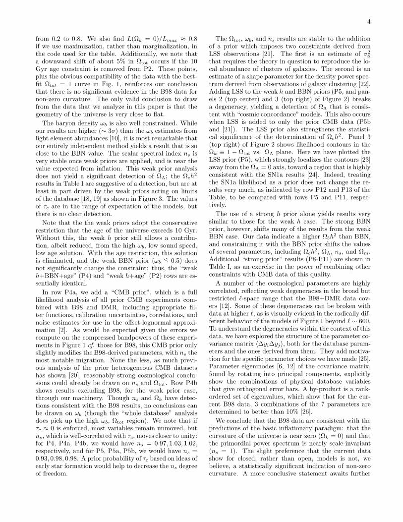
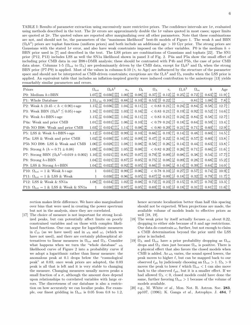
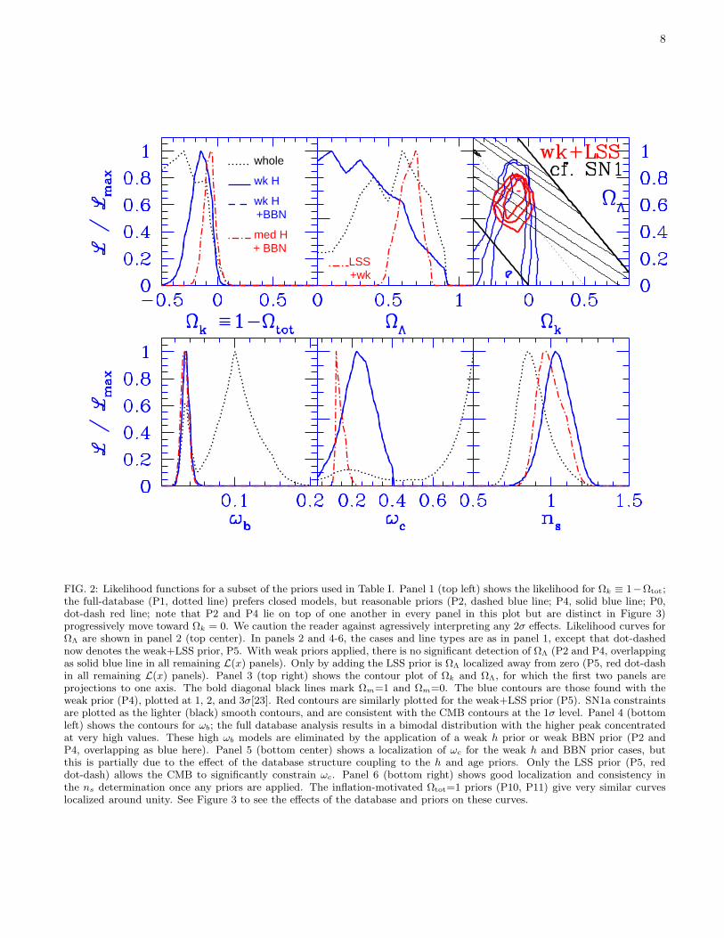