arX

iv:h

ep-t

h/03

1120

1v3

10

Jan

2004

Flavoring the gravity dual of N = 1 Yang-Mills

with probes

Carlos Nunez † 1, Angel Paredes ∗ 2 and Alfonso V. Ramallo ∗ 3

† Center for Theoretical Physics, Massachusetts Institute of TechnologyCambridge, MA 02139, USA

∗Departamento de Fısica de Partıculas, Universidad de Santiago de CompostelaE-15782 Santiago de Compostela, Spain

ABSTRACT

We study two related problems in the context of a supergravity dual to N = 1 SYM. Oneof the problems is finding kappa symmetric D5-brane probes in this particular background.The other is the use of these probes to add flavors to the gauge theory. We find a rich andmathematically appealing structure of the supersymmetric embeddings of a D5-brane probein this background. Besides, we compute the mass spectrum of the low energy excitationsof N = 1 SQCD (mesons) and match our results with some field theory aspects known fromthe study of supersymmetric gauge theories with a small number of flavors.

US-FT-3/03MIT-CPT/3441hep-th/0311201 November 2003

1nunez@lns.mit.edu2angel@fpaxp1.usc.es3alfonso@fpaxp1.usc.es

1 Introduction

The gauge/string correspondence, an old proposal due to ’t Hooft [1], is now well understoodin the context of maximally supersymmetric super Yang-Mills (SYM) theories. Indeed, theso-called AdS/CFT correspondence is a conjectured equivalence between type IIB stringtheory on AdS5 × S5 and N = 4 SYM theory [2]. In the large ’t Hooft coupling limit, theN = 4 SYM theory is dual to the type IIB supergravity background corresponding to thenear-horizon geometry of a stack of parallel D3-branes, whose metric is precisely that of theAdS5 × S5 space. There are nowadays a lot of non-trivial tests of this duality (for a reviewsee [3]).

The extension of the gauge/string correspondence to theories with less supersymmetriesis obviously of great interest. A possible way to obtain supergravity duals of SYM theorieswith reduced supersymmetry is to consider branes wrapping supersymmetric cycles of Calabi-Yau manifolds [4]. In order to preserve some supersymmetry the normal bundle of the cyclewithin the Calabi-Yau space has to be twisted [5]. Gauged supergravities in lower dimensionsprovide the most natural framework to implement this twisting. In these theories the gaugefield can be used to fiber the cycle in which the brane is wrapped in such a way that somesupersymmetries are preserved.

In this paper we will restrict ourselves to the case of the supergravity dual of N = 1 SYM.This background, which corresponds to a fivebrane wrapping a two-cycle, was obtained inref. [6] from the solution found in ref. [7] representing non-abelian magnetic monopolesin four dimensions. The geometry of this background is smooth and leads to confinementand chiral symmetry breaking. Actually, if only the abelian part of the vector field of sevendimensional gauged supergravity is excited, one obtains a geometry which is singular atthe origin and coincides with the smooth one at large distances, i.e. in the UV. Therefore,the singularity at the origin is resolved by making the gauge field non-abelian, in completeanalogy to what happens with the resolution of the Dirac string by the ’t Hooft-Polyakovmonopole. Moreover, as argued in ref. [8], the same mechanism that de-singularizes thesupergravity solution also gives rise to gaugino condensation. Based on this observation, theNSVZ beta function can be reproduced at leading order [9, 10, 11]. Other aspects of thissupergravity dual have been studied in ref. [12](for a review see [13]).

Most of the analysis carried out with the background of [6] do not incorporate quarks inthe fundamental representation which, in a string theory setup, correspond to open strings.In order to introduce an open string sector in a supergravity dual it is quite natural to add D-brane probes and see whether one can extract some information about the quark dynamics.As usual, if the number of brane probes is much smaller than those of the background, onecan assume that there is no backreaction of the probe in the bulk geometry. In this paperwe follow this approach and we will probe with D5-branes the supergravity dual of N = 1SYM. The main technique to determine the supersymmetric brane probe configurations iskappa symmetry [14], which tells us that, if ǫ is a Killing spinor of the background, onlythose embeddings for which a certain matrix Γκ satisfies

Γκ ǫ = ǫ . (1.1)

preserve the supersymmetry of the background [15]. The matrix Γκ depends on the metric

1

induced on the worldvolume of the brane. Therefore, if the Killing spinors ǫ are known, wecan regard (1.1) as an equation for the embedding of the brane.

The starting point in our program will be the determination of the Killing spinors ofthe background. It turns out that a simple expression for these spinors can be obtained ifone considers a frame inspired by the uplifting of the metric from gauged seven dimensionalsupergravity. The realization of the topological twist in this case is similar to the oneintroduced in ref. [16], which generalizes that of ref. [17], to obtain manifolds of G2 holonomyand the deformed and resolved conifold from gauged eight-dimensional supergravity. Theresulting Killing spinors are characterized by a series of projections and all we have to do isto find those configurations for which the kappa symmetry condition (1.1) follows from theprojections satisfied by the Killing spinors.

The probes we are going to consider are D5-branes wrapped on a two-dimensional sub-manifold. We will be able to find some differential equations for the embedding which are,in general, quite complicated to solve. The first obvious configuration one should look at isthat of a fivebrane wrapped at a fixed distance from the origin. In this case the equationssimplify drastically and we will be able to prove a no-go theorem which states that, unlesswe place the brane at an infinite distance from the origin, the probe breaks supersymmetry.This result is consistent with the fact that these N = 1 theories do not have a moduli space.In this analysis we will make contact with the two-cycle considered in ref. [10] and showthat it preserves supersymmetry at an asymptotically large distance from the origin.

Guided by the negative result obtained when trying to wrap the D5-brane at constantdistance, we will allow this distance to vary within the two-submanifold of the embedding. Tosimplify the equations that determine the embeddings, we first consider the singular versionof the background, in which the vector field of the seven dimensional gauged supergravity isabelian. This geometry coincides with the non-singular one, in which the vector field is non-abelian, at large distances from the origin. By choosing an appropriate set of variables we willbe able to write the differential equations for the embedding as two pairs of Cauchy-Riemannequations which are straightforward to integrate in general. Among all possible solutionswe will concentrate on some of them characterized by integers, which can be interpreted aswinding numbers. Generically these solutions have spikes, in which the probe is at infinitedistance from the origin and, thus, they correspond to fivebranes wrapping a non compactsubmanifold. Moreover, these configurations are worldvolume solitons and we will verifythat they saturate an energy bound [18].

With the insight gained by the analysis of the worldvolume solitons in the abelian back-ground we will consider the equations for the embeddings in the non-abelian background.In principle any solution for the smooth geometry must coincide in the UV with one of theconfigurations found for the singular metric. This observation will allow us to formulate anansatz to solve the complicated equations arising from kappa symmetry. Actually, in somecases, we will be able to find analytical solutions for the embeddings, which behave as thosefound for the singular metric at large distance from the origin and also saturate an energybound, which ensures their stability.

One of our motivations to study brane probes is to use these results to explore the quarksector of the gauge/gravity duality. Actually, it was proposed in refs. [19, 20] that one canadd flavor to this correspondence by considering spacetime filling branes and looking at their

2

fluctuations. In ref. [21] this program has been made explicit for the AdS5 × S5 geometryof a stack of D3-branes and a D7-brane probe. When the D3-branes of the background andthe D7-brane of the probe are separated, the fundamental matter arising from the stringsstretched between them becomes massive and a discrete spectrum of mesons for an N = 2SYM with a matter hypermultiplet can be obtained analytically from the fluctuations of a D7-brane probe. In ref. [22] a similar analysis was performed for the N = 1 Klebanov-Strasslerbackground [23], while in refs. [24, 25] the meson spectrum for some non-supersymmetricbackgrounds was found (for recent related work see refs. [26, 27]).

It was suggested in ref. [28] that one possible way to add flavor to the N = 1 SYMbackground is by considering supersymmetric embeddings of D5-branes which wrap a two-dimensional submanifold and are spacetime filling. Some of the configurations we will findin our kappa symmetry analysis have the right ingredients to be used as flavor branes. Theyare supersymmetric by construction, extend infinitely and have some parameter which deter-mines the minimal distance between the brane probe and the origin. This distance should beinterpreted as the mass scale of the quarks. Moreover, these brane probes capture geomet-rically the pattern of R-symmetry breaking of SQCD with few flavors [29]. Consequently,we will study the quadratic fluctuations around the static probe configurations found byintegrating the kappa symmetry equations. We will verify that these fluctuations decayexponentially at large distances. However, we will not be able to define a normalizabilitycondition which could give rise to a discrete spectrum. The reason for this is the exponentialblow up of the dilaton at large distances. Actually, this same difficulty was found in ref.[30] in the study of the glueball spectrum for this background. As proposed in ref. [30], weshall introduce a cut-off and impose boundary conditions which ensure that the fluctuationtakes place in a region in which the supergravity approximation remains valid. The resultingspectrum is discrete and, by using numerical methods, we will be able to determine its form.

The organization of this paper is the following. In section 2 we introduce the supergravitydual of N = 1 SYM. The Killing spinors for this background are obtained in appendix A,where we also obtain those corresponding to the background of refs. [31, 32, 33], whichrepresents D5-branes wrapped on a three-cycle. In section 3 we obtain the kappa symmetryequations which determine the supersymmetric embeddings. In section 4 we obtain the no-gotheorem for branes wrapped at fixed distance. In section 5 the kappa symmetry equationsfor the abelian background are integrated in general and some of the particular solutions arestudied in detail. Section 6 deals with the integration of the equations for the supersymmetricembeddings in the full non-abelian background. The spectrum of the quadratic fluctuationsis analysed in section 7. The asymptotic form of these fluctuations is obtained in appendixB. Finally, in section 8 we summarize our results, draw some conclusions and discuss somelines of future work.

1.1 Reader’s guide

Given that this is a long paper, we feel it would be useful to include here a “roadmap”to help the reader to quickly find the results of his/her particular interest. Those readersinterested in the supersymmetry preserved by the background and in the application of kappasymmetry to find compact and non compact embeddings in the geometry dual to N = 1

3

SYM, should pay special attention to sections 2-6 and appendix A. Readers more interestedin the gravity version of the addition of flavors to N = 1 SYM should take for granted section3 and look at the solutions exhibited in eqs. (5.19), (5.22) and (6.15), which are what wecalled “abelian and non-abelian unit-winding solutions”. Then, they should go straight tosection 7 and take into account the results of appendix B.

2 The supergravity dual of N = 1 Yang-Mills

The supergravity solution we will be dealing with corresponds to a stack of N D5-braneswrapped on a two-cycle. It can be obtained [6, 7] by considering seven dimensional gaugedsupergravity, which is a consistent truncation of ten dimensional supergravity on a three-sphere. To get this background one starts with an ansatz for the seven dimensional metricwhich has a term corresponding to the metric of a two-sphere and looks for a supersymmetricsolution of the equations of motion. After uplifting to ten dimensions one ends up with asolution of type IIB supergravity which preserves four supersymmetries. The ten dimensionalmetric in Einstein frame is:

ds210 = e

φ

2

[

dx21,3 + e2h ( dθ2 + sin2 θdϕ2 ) + dr2 +

1

4(wi −Ai)2

]

, (2.1)

where φ is the dilaton, the unwrapped coordinates xµ have been rescaled and all distancesare measured in units of Ngsα

′. The angles θ ∈ [0, π] and ϕ ∈ [0, 2π) parametrize thetwo-sphere of gauged seven dimensional supergravity. This sphere is fibered in the tendimensional metric by the one-forms Ai (i = 1, 2, 3), which are the components of the non-abelian gauge vector field of the seven dimensional supergravity. Their expression can bewritten in terms of a function a(r) and the angles (θ, ϕ) as follows:

A1 = −a(r)dθ , A2 = a(r) sin θdϕ , A3 = − cos θdϕ . (2.2)

The wi ’s appearing in eq. (2.1) are the su(2) left-invariant one-forms, satisfying dwi =−1

2ǫijk w

j ∧wk, which parametrize the compactification three-sphere and can be represented

in terms of three angles ϕ, θ and ψ:

w1 = cosψdθ + sinψ sin θdϕ ,

w2 = − sinψdθ + cosψ sin θdϕ ,

w3 = dψ + cos θdϕ . (2.3)

The three angles ϕ, θ and ψ take values in the rank 0 ≤ ϕ < 2π, 0 ≤ θ ≤ π and 0 ≤ ψ < 4π.For a metric ansatz such as the one written in (2.1) one obtains a supersymmetric solutionwhen the functions a(r), h(r) and the dilaton φ are:

a(r) =2r

sinh 2r,

4

e2h = r coth 2r − r2

sinh2 2r− 1

4,

e−2φ = e−2φ02eh

sinh 2r, (2.4)

where φ0 is the value of the dilaton at r = 0. Near the origin r = 0 the function e2h behavesas e2h ∼ r2 and the metric is non-singular. The solution of the type IIB supergravity includesa Ramond-Ramond three-form F(3) given by

F(3) = −1

4(w1 − A1 ) ∧ (w2 − A2 ) ∧ (w3 − A3 ) +

1

4

∑

a

F a ∧ (wa − Aa ) , (2.5)

where F a is the field strength of the su(2) gauge field Aa, defined as:

F a = dAa +1

2ǫabc A

b ∧Ac . (2.6)

The different components of F a are:

F 1 = −a′ dr ∧ dθ , F 2 = a′ sin θdr ∧ dϕ , F 3 = ( 1 − a2 ) sin θdθ ∧ dϕ , (2.7)

where the prime denotes derivative with respect to r. Since dF(3) = 0, one can represent F(3)

in terms of a two-form potential C(2) as F(3) = dC(2). Actually, it is not difficult to verifythat C(2) can be taken as:

C(2) =1

4

[

ψ ( sin θdθ ∧ dϕ − sin θdθ ∧ dϕ ) − cos θ cos θdϕ ∧ dϕ −

−a ( dθ ∧ w1 − sin θdϕ ∧ w2 )]

. (2.8)

Moreover, the equation of motion of F(3) in the Einstein frame is d(

eφ ∗F(3)

)

= 0, where ∗denotes Hodge duality. Therefore it follows that, at least locally, one must have

eφ ∗F(3) = dC(6) , (2.9)

with C(6) being a six-form potential. It is readily checked that C(6) can be taken as:

C(6) = dx0 ∧ dx1 ∧ dx2 ∧ dx3 ∧ C , (2.10)

where C is the following two-form:

C = −e2φ

8

[ (

( a2 − 1 )a2 e−2h − 16 e2h)

cos θdϕ ∧ dr − ( a2 − 1 ) e−2hw3 ∧ dr +

+ a′(

sin θdϕ ∧ w1 + dθ ∧ w2) ]

. (2.11)

5

The Killing spinors ǫ of the above background are worked out in Appendix A. They canbe obtained by requiring the vanishing of the supersymmetry variations of the fermionicfields of type IIB supergravity. This requirement leads to a system of first-order BPS dif-ferential equations (eq. (A.16)) for the functions φ, h and a of the ansatz written in eqs.(2.1) and (2.5). It can be easily checked that the functions of eq. (2.4) satisfy the system(A.16). Moreover, it follows from the analysis of appendix A that the Killing spinors ǫ arecharacterized by the following set of projections:

Γx0···x3 ( cosαΓ12 + sinαΓ1Γ2 ) ǫ = ǫ ,

Γ12 ǫ = Γ12 ǫ ,

ǫ = iǫ∗ , (2.12)

where the Γ-matrices refer to the frame (A.2) and the explicit expression of the angle α,which depends on the radial coordinate r, is given in eqs. (A.17) and (A.25) (see eqs. (A.3),(A.4) and (A.26)). It is interesting to write here the UV and IR limits of α, namely

limr→∞

α = 0 , limr→0

α = −π2. (2.13)

The BPS equations (A.16) also admit a solution in which the function a(r) vanishes, i.e.

in which the one-form Ai has only one non-vanishing component, namely A3. We will referto this solution as the abelian N = 1 background. Its explicit form can be easily obtainedby taking the r → ∞ limit of the functions given in eq. (2.4). Notice that, indeed a(r) → 0as r → ∞ in eq. (2.4). Neglecting exponentially suppressed terms, one gets:

e2h = r − 1

4, (a = 0) , (2.14)

while φ can be obtained from the last equation in (2.4). The metric of the abelian backgroundis singular at r = 1/4 (the position of the singularity can be moved to r = 0 by a redefinitionof the radial coordinate). This IR singularity of the abelian background is removed in thenon-abelian metric by switching on the A1, A2 components of the one-form (2.2). Moreover,when a = 0, the angle α appearing in the expression of the Killing spinors (and in theprojection (2.12)) is zero, as follows from eq. (A.17).

3 Kappa symmetry

As mentioned in the introduction, the kappa symmetry condition for a supersymmetricembedding of a D5-brane probe is Γκ ǫ = ǫ (see eq. (1.1)), where ǫ is a Killing spinor of thebackground. For ǫ such that ǫ = iǫ∗ and when there is no worldvolume gauge field, one has:

Γκ =1

6!

1√−g ǫm1···m6 γm1···m6 , (3.1)

6

where g is the determinant of the induced metric gmn on the worldvolume

gmn = ∂mXµ ∂nX

ν Gµν , (3.2)

with Gµν being the ten-dimensional metric and γm1···m6 are antisymmetrized products ofworldvolume Dirac matrices γm, defined as:

γm = ∂mXµEν

µ Γν . (3.3)

The vierbeins Eνµ are the coefficients which relate the one-forms eν of the frame and the

differentials of the coordinates, i.e. eν = EνµdX

µ. Let us take as worldvolume coordinates

(x0, · · · , x3, θ, ϕ). Then, for an embedding with θ = θ(θ, ϕ), ϕ = ϕ(θ, ϕ), ψ = ψ(θ, ϕ) andr = r(θ, ϕ), the kappa symmetry matrix Γκ takes the form:

Γκ =eφ

√−g Γx0···x3 γθϕ , (3.4)

with γθϕ being the antisymmetrized product of the two induced matrices γθ and γϕ, whichcan be written as:

e−φ

4 γθ = eh Γ1 + (V1θ +a

2) Γ1 + V2θ Γ2 + V3θ Γ3 + ∂θrΓr ,

e−φ

4

sin θγϕ = eh Γ2 + V1ϕ Γ1 + (V2ϕ − a

2) Γ2 + V3ϕ Γ3 +

∂ϕr

sin θΓr , (3.5)

where the V ’s can be obtained by computing the pullback on the worldvolume of the leftinvariant one-forms wi, and are given by:

V1θ =1

2cosψ ∂θ θ +

1

2sinψ sin θ ∂θ ϕ ,

sin θ V1ϕ =1

2cosψ ∂ϕ θ +

1

2sinψ sin θ ∂ϕ ϕ ,

V2θ = −1

2sinψ ∂θ θ +

1

2cosψ sin θ ∂θ ϕ ,

sin θ V2ϕ = −1

2sinψ ∂ϕ θ +

1

2cosψ sin θ ∂ϕ ϕ ,

V3θ =1

2∂θψ +

1

2cos θ ∂θ ϕ ,

sin θ V3ϕ =1

2∂ϕψ +

1

2cos θ ∂ϕ ϕ +

1

2cos θ . (3.6)

By using the projections (A.3) and (A.8) one can compute the action of γθϕ on the Killingspinor ǫ. It is clear that one arrives at an expression of the type:

e−φ

2

sin θγθϕ ǫ = [ c12 Γ12 + c12 Γ1Γ2 + c11 Γ1Γ1 + c13 Γ1Γ3 +

+ c13 Γ13 + c23 Γ23 + c23 Γ2Γ3 ] ǫ , (3.7)

7

where the c’s are coefficients that can be explicitly computed. By using eq. (3.7) we canobtain the action of Γκ on ǫ and we can use this result to write the kappa symmetry projectionΓκǫ = ǫ. Actually, eq. (1.1) is automatically satisfied if it reduces to the first equation in eq.(2.12). If we want this to happen, all terms except the ones containing Γ12 ǫ and Γ1 Γ2 ǫ onthe right-hand side of eq. (3.7) should vanish. Then, we should require

c11 = c13 = c13 = c23 = c23 = 0 . (3.8)

By using the explicit expressions of the c’s one can obtain from eq. (3.8) five conditions thatour supersymmetric embeddings must necessarily satisfy. These conditions are:

eh (V1ϕ + V2θ ) = 0 , (3.9)

eh (V3ϕ + cosα∂θr ) + (V2ϕ − a

2) sinα∂θr − V2θ sinα

∂ϕr

sin θ= 0 , (3.10)

(V1θ +a

2)V3ϕ − V3θ V1ϕ − eh sinα∂θr +

+ (V2ϕ − a

2) cosα∂θr − V2θ cosα

∂ϕr

sin θ= 0 , (3.11)

V3ϕ V2θ − V3θ (V2ϕ − a

2) − V1ϕ cosα∂θr +

+(

eh sinα + (V1θ +a

2) cosα

)

∂ϕr

sin θ= 0 , (3.12)

sinαV1ϕ∂θr − eh V3θ +(

eh cosα − (V1θ +a

2) sinα

)

∂ϕr

sin θ= 0 . (3.13)

Moreover, if we want the kappa symmetry projection Γκǫ = ǫ to coincide with the SUGRAprojection, the ratio of the coefficients of the terms with Γ1 Γ2 ǫ and Γ12 ǫ must be tanα, i.e.

one must have:

tanα =c12c12

. (3.14)

The explicit form of c12 and c12 is:

c12 = e2h + V1θ V2ϕ − V2θ V1ϕ − a

2(V1θ − V2ϕ ) − a2

4− cosαV3ϕ ∂θr + cosαV3θ

∂ϕr

sin θ,

c12 = eh (V2ϕ − V1θ − a ) − sinαV3ϕ ∂θr + sinαV3θ∂ϕr

sin θ. (3.15)

Amazingly, except when r is constant and takes values in the interval 0 < r <∞ (see section4), eq. (3.14) is a consequence of eqs. (3.9)-(3.13). Actually, by eliminating V3θ of eqs. (3.12)and (3.13), and making use of eqs. (3.9) and (3.10), one arrives at the following expressionof tanα:

tanα =eh (V2ϕ − V1θ − a )

e2h + V1θ V2ϕ − V2θ V1ϕ − a2(V1θ − V2ϕ ) − a2

4

. (3.16)

8

Notice that the terms of c12 (c12) which do not contain sinα (cosα) are just the ones in thenumerator (denominator) of the right-hand side of this equation. It follows from this factthat eq. (3.14) is satisfied if eqs. (3.9)-(3.13) hold. Moreover, by using the values of cosαand sinα given in eq. (A.17), one obtains the interesting relation:

(

1 + a2 + 4e2h ) (V1θ − V2ϕ ) = 4a(

V 22θ + V1θ V2ϕ − 1

4

)

. (3.17)

The system of eqs. (3.9)-(3.13) is rather involved and, although it could seem at first sightvery difficult and even hopeless to solve, we will be able to do it in some particular cases.Moreover, it is interesting to notice that, by simple manipulations, one can obtain the fol-lowing expressions of the partial derivatives of r:

∂θr = − cosαV3ϕ + sinα e−h [ (V1θ +a

2)V3ϕ − V3θ V1ϕ ] ,

∂ϕr = cosα sin θV3θ + sinα sin θe−h [ (V2ϕ − a

2)V3θ − V3ϕ V2θ ] , (3.18)

which will be very useful in our analysis.

4 Branes wrapped at fixed distance

In this section we will consider the possibility of wrapping the D5-branes at a fixed distancer > 0 from the origin. It is clear that, in this case, we have ∂θr = ∂ϕr = 0 and many ofthe terms on the left-hand side of eqs. (3.9)-(3.13) cancel. Moreover eh is non-vanishingwhen r > 0 and it can be factored out in these equations. Thus, the equations (3.9)-(3.13)of kappa symmetry when the radial coordinate r is constant and non-zero reduce to:

V1ϕ + V2θ = V3ϕ = V3θ = 0 . (4.1)

From the equations V3ϕ = V3θ = 0 we obtain the following differential equations for ψ

∂θ ψ = − cos θ ∂θϕ , ∂ϕ ψ = − cos θ ∂ϕϕ − cos θ . (4.2)

The integrability condition for this system gives:

∂ϕθ ∂θϕ − ∂θθ ∂ϕϕ =sin θ

sin θ. (4.3)

By using this condition and the definition of the V ’s (eq. (3.6)) one can prove that

V1θ V2ϕ − V1ϕ V2θ = −1

4. (4.4)

Let us now define ∆ as follows:V2ϕ − V1θ ≡ ∆ . (4.5)

9

By using the expression of the V’s in terms of the angles, one can combine eq. (4.5) and thecondition V1ϕ + V2θ = 0 in the following matrix equation

cosψ sinψ

− sinψ cosψ

sin θ∂θ θ − sin θ∂ϕϕ

sin θ sin θ∂θϕ + ∂ϕθ

=

−2∆ sin θ

0

. (4.6)

Since the matrix appearing on the left-hand side is non-singular, we can multiply by itsinverse. By doing this one arrives at the following equations:

∂θθ − sin θ

sin θ∂ϕϕ = −2∆ cosψ ,

∂ϕθ

sin θ+ sin θ∂θϕ = −2∆ sinψ . (4.7)

Substituting the derivatives of θ obtained from the above equations into the integrabilitycondition (4.3) we obtain after some calculation

sin2 θ

(

∂θϕ + ∆sinψ

sin θ

)2

+sin2 θ

sin2 θ

(

∂ϕϕ − ∆ cosψsin θ

sin θ

)2

= ∆2 − 1 . (4.8)

The right-hand side of eq. (4.8) is non-negative. Then, one obtains a bound for ∆:

∆2 ≥ 1 . (4.9)

Notice that we have not imposed all the requirements of kappa symmetry. Indeed, it stillremains to check that the ratios between the coefficients c12 and c12 is the one correspondingto the projection of the background. Using eq. (4.4) and the definition of ∆ (eq. 4.5)), oneobtains:

c12 = e2h + a∆

2− a2 + 1

4, c12 = eh (∆ − a) . (4.10)

Then, one must have:

tanα =eh (∆ − a)

e2h + a ∆2− a2+1

4

= − aeh

e2h + 1−a2

4

, (4.11)

where we have used the values of sinα and cosα given in the appendix A (eq. A.17). If eh

is nonzero (and finite), we can factor it out in eq. (4.11) and obtain the following expressionof ∆:

∆ =2a

1 + a2 + 4e2h. (4.12)

Notice that ∆ depends only on the coordinate r and is a monotonically decreasing functionsuch that 0 < ∆ < 1 for 0 < r <∞ and

limr→0

∆ = 1 , limr→∞

∆ = 0 . (4.13)

10

As ∆ < 1, the bound (4.9) is not satisfied and, thus, there is no solution to our equationsfor 0 < r < ∞. Notice that this was to be expected from the lack of moduli space of theN = 1 theories.

Let us now consider the possibility of placing the brane probe at r → ∞. Notice that inthis case eq. (4.11) is satisfied for any finite value of ∆. However, the value ∆ = 1 is specialsince, in this case, the right-hand side of eq. (4.8) vanishes and we obtain two equations thatdetermine the derivatives of ϕ, namely:

∂θϕ = −sinψ

sin θ, ∂ϕϕ = cosψ

sin θ

sin θ(4.14)

Using these equations into the system (4.7) for ∆ = 1 one gets the following equations forthe derivatives of θ:

∂θθ = − cosψ , ∂ϕθ = − sin θ sinψ , (4.15)

and, similarly, the equations (4.2) for ψ become:

∂θψ = sinψ cot θ , ∂ϕψ = − sin θ cot θ cosψ − cos θ (4.16)

The equations (4.14) and (4.15) can be regarded as coming from the following identificationsof the frame forms in the (θ, ϕ) and (θ, ϕ) spheres:

dθ

sin θdϕ

=

cosψ − sinψ

sinψ cosψ

−dθ

sin θdϕ

(4.17)

The differential equations (4.16) are just the integrability conditions of the system (4.17).Another interesting observation is that one can prove by using the differential eqs. (4.14)-(4.16) that the pullbacks of the su(2) left-invariant one-forms are

P [w1] = −dθ , P [w2] = sin θdϕ , P [w3] = − cos θdϕ . (4.18)

Let us try to find a solution of the differential equations (4.14)-(4.16) in which θ = θ(θ)and ϕ = ϕ(ϕ). The vanishing of ∂ϕθ and ∂θϕ immediately leads to sinψ = 0 or ψ =0, π (mod 2π). Thus ψ is constant in this case. Let us put cosψ = η = ±1. The vanishingof ∂θψ is automatic, whereas the condition ∂ϕψ = 0 leads to a relation between θ and θ:

cot θ = −η cot θ (4.19)

In the case ψ = 0, one has η = 1 and the previous relation yields θ = π− θ. Notice that thisrelation is in agreement with the first equation in eq. (4.15). Moreover, the second equationin (4.14) gives ϕ = ϕ. Similarly one can solve the equations for ψ = π. The solutions inthese two cases are just the ones used in ref. [10] in the calculation of the beta function(with some correction in the ψ = 0 case to have the correct range of θ and θ), namely:

θ = π − θ , ϕ = ϕ , ψ = 0 (mod 2π) ,

θ = θ , ϕ = 2π − ϕ , ψ = π (mod 2π) (4.20)

11

It follows from our results that the embedding of ref. [10] is only supersymmetric asymp-totically when r → ∞. In this sense, although it is somehow distinguished, it is not uniquesince for any embedding such that the V ’s are finite when r → ∞, the determinant of the

induced metric diverges as√−g ∼ e

3φ

2+2h and the only term which survives in the equation

Γκǫ = ǫ is the one with the matrix Γ12, giving rise to the same projection as the backgroundfor r → ∞.

5 Worldvolume solitons (abelian case)

Let us consider the case a = α = 0 in the general equations of section 3. From equations(3.9) and (3.17) we get the following (Cauchy-Riemann like) equations:

V1θ = V2ϕ , V1ϕ = −V2θ , (5.1)

whereas, from eq. (3.18) we obtain that the derivatives of r are given by:

rθ = −V3ϕ , rϕ = sin θ V3θ , (5.2)

where rθ ≡ ∂θr and rϕ ≡ ∂ϕr. It can be easily demonstrated that, in this abelian case,the full set of equations (3.9)-(3.13) collapses to the two pairs of equations (5.1) and (5.2).Notice that c12 = 0 when a = α = 0 and eq. (5.1) holds and, thus, eq. (3.14) is satisfiedidentically.

Let us study first the two equations (5.1). By using the same technique as the oneemployed in section 4 to derive eq. (4.7), it can be shown easily that they can be written as

sin θ∂θ θ = sin θ∂ϕϕ , ∂ϕθ = − sin θ sin θ∂θϕ . (5.3)

In order to find the general solution of eq. (5.3), let us introduce a new set of variables uand u as follows:

u = log tanθ

2, u = log tan

θ

2. (5.4)

Then, eq. (5.3) can be written as the Cauchy-Riemann equations in the (u, ϕ) and (u, ϕ)variables, namely:

∂u

∂u=

∂ϕ

∂ϕ,

∂u

∂ϕ= −∂ϕ

∂u. (5.5)

Since u, u ∈ (−∞,+∞) and ϕ, ϕ ∈ (0, 2π), the above equations are the Cauchy-Riemannequations in a band. The general solution of these equations is of the form:

u+ iϕ = f(u+ iϕ) , (5.6)

where f is an arbitrary function. Given any function f , it is clear that the above equationprovides the general solution θ(θ, ϕ) and ϕ(θ, ϕ) of the system (5.3).

12

Let us turn now to the analysis of the system of equations (5.2), which determines theradial coordinate r. By using the explicit values of V3ϕ and V3θ, these equations can bewritten as:

rθ = − 1

2 sin θ∂ϕ ψ − 1

2

cos θ

sin θ∂ϕϕ− 1

2cot θ ,

rϕ =sin θ

2∂θ ψ +

sin θ

2cos θ ∂θϕ , (5.7)

where θ(θ, ϕ) and ϕ(θ, ϕ) are solutions of eq. (5.3). In terms of the derivatives with respectto variable u defined above (sin θ∂θ = ∂u), these equations become:

ru = −1

2∂ϕψ − 1

2cos θ ∂ϕϕ − 1

2cos θ ,

rϕ =1

2∂uψ +

1

2cos θ ∂uϕ . (5.8)

The integrability condition of these equations is just ∂ϕru = ∂urϕ. As any solution (θ, ϕ) ofthe Cauchy-Riemann equations (5.3) satisfies:

∂ϕθ∂ϕϕ = −∂uθ∂uϕ , (5.9)

and, since ϕ, being a solution of the Cauchy-Riemann equations, is harmonic in (u, ϕ), itfollows that ∂ϕru = ∂urϕ if and only if ψ is also harmonic in (u, ϕ), i.e. the differentialequation for ψ is just the Laplace equation in the (u, ϕ) plane, namely

∂2ϕψ + ∂2

uψ = 0 . (5.10)

Remarkably, the form of r(θ, ϕ) can be obtained in general. Let us define:

Λ(θ, ϕ) =∫ ϕ

0dϕ sin θ∂θψ(θ, ϕ) −

∫ dθ

sin θ∂ϕψ(θ, 0) , (5.11)

It follows from this definition and the fact that ψ is harmonic in (u, ϕ) that ψ and Λ alsosatisfy the Cauchy-Riemann equations:

∂Λ

∂ϕ=

∂ψ

∂u,

∂Λ

∂u= −∂ψ

∂ϕ. (5.12)

Thus ψ and Λ are conjugate harmonic functions, i.e. ψ+ iΛ is an analytic function of u+ iϕ.Notice that given Λ one can obtain ψ by integrating the previous differential equations. Itcan be checked by using the Cauchy-Riemann equations that the derivatives of r, as givenby the right hand side of eq. (5.8), can be written as rθ = ∂θF , rϕ = ∂ϕF , where:

F (θ, ϕ) =1

2

[

Λ(θ, ϕ) − log ( sin θ sin θ(θ, ϕ))]

. (5.13)

Therefore, it follows that:

e2r = CeΛ(θ,ϕ)

sin θ sin θ(θ, ϕ), (5.14)

with C being a constant. We will make use of this amazingly simple expression to derive theequation of some particularly interesting embeddings.

13

-6 -4 -2 2 4 6

y

x

Figure 1: Curves y = y(x) for three values of the winding number n: n = 0 (solid line),n = 1 (dashed curve) and n = 2 (dotted line). These three curves correspond to r∗ = 1.

5.1 n-Winding solitons

First of all, let us consider the particular class of solutions of the Cauchy-Riemann eqs. (5.5):

u+ iϕ = n(u+ iϕ) + constant , (5.15)

where n is an integer and the constant is complex. In terms of the original variables:

tanθ

2= c

(

tanθ

2

)n

, ϕ = nϕ + ϕ0 , (5.16)

with c and ϕ0 being constants. It is clear that in this solution the ϕ coordinate of the probewraps n times the [0, 2π] interval as ϕ varies between 0 and 2π. Let us now assume that thecoordinate ψ is constant, i.e. ψ = ψ0. It is clear from its definition that the function Λ(θ, ϕ)is zero in this case. Moreover, by using the identities

sin x =2 tan x

2

1 + tan2 x2

, tanx

2=

√

1 − cosx

1 + cosx, (5.17)

one can prove that:

sin θ = 2√c

(sin θ )n

( 1 + cos θ )n + c ( 1 − cos θ )n, (5.18)

where c = c2. After plugging this result in eq. (5.14), one obtains the explicit form of thefunction r(θ), namely:

e2r =e2r∗

1 + c

( 1 + cos θ )n + c ( 1 − cos θ )n

(sin θ )n+1, (5.19)

where r∗ = r(θ = π/2). We will call n-winding embedding to the brane configurationcorresponding to eqs. (5.16) and (5.19) for a constant value of the angle ψ.

Let us pause for a moment to study the function (5.19). First of all it is easy to verifythat this function is invariant if we change n → −n and c → 1/c (or equivalently changingθ → π − θ for the same constant c). Actually, in what follows we shall take the integrationconstant c = 1 and thus we can restrict ourselves to the case in which n is non-negative.In this c = 1 case r∗ is the minimal separation between the brane probe and the origin.

14

Another observation is that r diverges for θ = 0, π, which corresponds to the location ofthe spikes of the worldvolume solitons. Therefore the supersymmetric embedding we havefound is non-compact. Actually, it has the topology of a cylinder whose compact directionis parametrized by ϕ. This cylinder connects the two poles at θ = 0, π of the (θ, ϕ) sphereat r = ∞ and passes at a distance r∗ from the origin.

It is also interesting to discuss the symmetries of our solutions. Recall that the angle ψ isconstant for our embeddings. Thus, it is clear that one can shift it by an arbitrary constantǫ as ψ → ψ + ǫ. This U(1) symmetry corresponds to an isometry of the abelian backgroundwhich quantum-mechanically is broken to ZZ 2N as a consequence of the flux quantizationof the RR two-form potential [6, 34, 35]. In the gauge theory side this isometry has beenidentified [6, 34, 35] with the U(1) R-symmetry of the N = 1 SYM theory, which is brokendown to ZZ 2N by a field theory anomaly [29]. On the other hand, it is also clear that we havean additional U(1) associated to constant shifts in ϕ, which are equivalent to a redefinitionof ϕ0 in eq. (5.16).

To visualize the shape of the brane in these solutions it is rather convenient to introducethe following cartesian coordinates x and y

x = r cos θ , y = r sin θ . (5.20)

In terms of (x, y) the D5-brane embedding will be described by means of a curve y = y(x).Notice that y ≥ 0, whereas −∞ < x < +∞. The value of the coordinate y at x = 0 is justr∗, i.e. y(x = 0) = r∗. Moreover, for large values of the coordinate x, the function y(x) → 0exponentially as

y(x) ≈ C |x| e− 2|n|+1

|x| , (|x| → ∞) , (5.21)

where C is a constant. To illustrate this behaviour we have plotted in figure 1 the curvesy(x) for three different values of the winding n and the same value of r∗.

A particularly interesting case is obtained when n = ±1. By adjusting properly theconstant ϕ0 in eq. (5.16) the angular embedding reduces to:

θ = θ , ϕ = ϕ + constant , (n = 1) ,

θ = π − θ , ϕ = 2π − ϕ + constant , (n = −1) , (5.22)

with ψ being constant. These types of angular embeddings are similar to the ones consideredin ref. [10] (although they are not the same, see eq. (4.20) ) and we will refer to them asunit-winding embeddings. Notice that the two cases displayed in eq. (5.22) represent thetwo possible identifications of the (θ, ϕ) and (θ, ϕ) two-spheres.

When n = 0 the brane is wrapping the (θ, ϕ) sphere at constant values of θ and ϕ, i.e.

one has:θ = constant = θ0 , ϕ = constant = ϕ0 , (n = 0) (5.23)

We will refer to this case as zero-winding embedding [9].One can verify that the brane embeddings we have found are solutions of the probe

equations of motion. Actually, they are supersymmetric worldvolume solitons of the D5brane probe. To illustrate this fact let us show that these configurations saturate a BPS

15

energy bound. To simplify matters, let us assume that the angular embedding is the onedisplayed in eq. (5.16) and let r(θ) be an arbitrary function. The Dirac-Born-Infeld (DBI)lagrangian density for a D5-brane with unit tension is:

L = −e−φ √−gst + P[

C(6)

]

, (5.24)

where gst is the determinant of the induced metric in the string frame (gst = e3φ g) and

P[

C(6)

]

is the pullback on the worldvolume of the RR six-form of the background. Theelements of the induced metric for the n-winding solution along the angular coordinates are:

gθθ = eφ

2

(

e2h +n2

4

sin2 θ

sin2 θ+ r2

θ

)

,

gϕϕ = eφ

2

(

e2h +n2

4

sin2 θ

sin2 θ+ V 2

3ϕ

)

sin2 θ . (5.25)

From this expression one immediately obtains the determinant of the induced metric, namely:

√−g = e3φ

2 sin θ

√

√

√

√

(

e2h +n2

4

sin2 θ

sin2 θ+ V 2

3ϕ

)(

e2h +n2

4

sin2 θ

sin2 θ+ r2

θ

)

. (5.26)

Moreover, the pullback on the worldvolume of the two-form C is 1:

P[

C]

=e2φ

8( 16e2h cos θ − ne−2h cos θ ) rθ dϕ ∧ dθ (5.27)

The hamiltonian density H for a static configuration is just H = −L or:

H = e2φ

[

sin θ

√

√

√

√

(

e2h +n2

4

sin2 θ

sin2 θ+ V 2

3ϕ

)(

e2h +n2

4

sin2 θ

sin2 θ+ r2

θ

)

−

− 1

8( 16e2h cos θ − ne−2h cos θ ) rθ

]

, (5.28)

It can be checked that, for an arbitrary function r(θ), one can write H as:

H = Z + S , (5.29)1It is worth mentioning that the pullback of the RR two-form to the worldvolume is

P [C(2)] =ψ

4dϕ ∧

(

n sin θdθ − sin θdθ)

,

where θ(θ) is the function displayed in eq. (5.18) . From this expression it is straightforward to verify thatthe RR two-form flux through the two-submanifold where we are wrapping our brane is

∫

P [C(2)] = πψ (|n| − 1) ,

and thus it vanishes iff n = ±1.

16

where Z is a total derivative:

Z = −∂θ

[

e2φ(

e2h cos θ +n

4cos θ

)

]

, (5.30)

and S is non-negative:S ≥ 0 , (5.31)

with S = 0 precisely when the BPS equations for the embedding are satisfied. The expressionof S is:

S = sin θ e2φ

[

√

√

√

√

(

e2h +n2

4

sin2 θ

sin2 θ+ V 2

3ϕ

)(

e2h +n2

4

sin2 θ

sin2 θ+ r2

θ

)

−

−(

e2h +n2

4

sin2 θ

sin2 θ− V3ϕ rθ

)

]

. (5.32)

The BPS equation for r in this case is rθ = −V3ϕ (see eq. (5.2)). If this equation is satisfied,the first term on the right-hand side of eq. (5.32) is a square root of a perfect square whichcancels against the second term of this equation. Moreover, it is easy to check that thecondition S ≥ 0 is equivalent to:

(rθ + V3ϕ )2 ≥ 0 , (5.33)

which is obviously satisfied and reduces to an equality if and only if the BPS equation forthe embedding is satisfied.

5.2 (n,m)-Winding solitons

The solutions found in the previous section are easily generalized if we allow the angle ψ towind a certain number of times as the coordinate ϕ varies from ϕ = 0 to ϕ = 2π. Recallingthat ψ ranges from 0 to 4π, let us write the following ansatz for ψ(ϕ):

ψ = ψ0 + 2mϕ , (5.34)

where m is an integer. It is obvious that the above function satisfies the Laplace equation(5.10). Moreover, its harmonic conjugate Λ is immediately obtained by solving the Cauchy-Riemann differential equations (5.12), namely:

Λ = −2mu . (5.35)

In terms of the angle θ, the above equation becomes:

eΛ =1

(

tan θ2

)2m . (5.36)

17

By plugging this result in eq. (5.14), and using the value of sin θ given in eq. (5.18), it isstraightforward to obtain the function r(θ) of the embedding. One gets:

e2r =e2r∗

1 + c

( 1 + cos θ )n + c ( 1 − cos θ )n

[ tan θ2]2m(sin θ )n+1

, (5.37)

where, as in the n-winding case, r∗ = r(θ = π/2).An interesting observation concerning the solution we have just found is that, by choosing

appropriately the winding number m, one of the spikes of the m = 0 solutions at θ = 0 orθ = π disappears. Indeed if, for example, n is nonnegative and we take 2m = n + 1, thefunction r(θ) is regular at θ = 0. Similarly, also when n ≥ 0, one can eliminate the spike atθ = π by choosing 2m = −n− 1.

5.3 Spiral solitons

By considering more general solutions of the Cauchy-Riemann equations (5.5) and (5.12) wecan obtain many more classes of supersymmetric configurations of the brane probe. One ofthe questions one can address is whether or not one can have embeddings in which r is finitefor all values of the angles. We will now see that the answer to this question is yes, althoughthe corresponding embeddings seem not to be very interesting. To illustrate this point, letus see how we can find functions ψ and Λ such that they make the radial coordinate of then-winding embedding finite at θ = 0, π. First of all, notice that, in terms of the Cauchy-Riemann variables u and u defined in eq. (5.4), we have to explore the behaviour of theembedding at u, u→ ±∞. Since

sin θ =2eu

1 + e2u, sin θ =

2eu

1 + e2u, (5.38)

one has that sin θ → e−|u|, sin θ → e−|u| as u, u → ±∞. Then, the factors multiplying eΛ

in eq. (5.14) diverge as e|u|+|u|. In the n-winding solution |u| = |n||u| and, therefore thisdivergence is of the type e(|n|+1)|u|. We can cancel this divergence by adding a Λ such thateΛ → 0 as u→ ±∞ in such a way that, for example, Λ + (|n|+ 1)|u| → −∞. This is clearlyachieved by taking a function Λ such that Λ → −u2. It is straightforward to find an analyticfunction in the (u, ϕ) plane such that its imaginary part behaves as −u2 for u→ ±∞. Onecan take

ψ + iΛ = −i(u + iϕ)2 = 2uϕ − i(u2 − ϕ2) . (5.39)

From this equation we can read the functions ψ and Λ. In terms of θ and ϕ they are:

ψ = 2uϕ = 2ϕ log tanθ

2, Λ = −u2 + ϕ2 = −( log tan

θ

2)2 + ϕ2 . (5.40)

In this case r → 0, ψ → ±∞ as θ → 0, π, which means that we describe an infinite spiralwhich winds infinitely in the ψ direction. Notice that, although r is always finite, the volumeof the two-submanifold is infinite due to this infinite winding. One can try other alternativesto make the radial coordinate finite. In all the ones we have analyzed one obtains the infinitespiral behaviour described above.

18

6 Worldvolume solitons (nonabelian case)

Let us consider the full nonabelian background and let us try to obtain solutions to thekappa symmetry equations (3.9)-(3.13). Actually we will restrict ourselves to the situationsin which r only depends on the angle θ. It can be easily checked that, in this case, only fourof the five equations (3.9)-(3.13) are independent. As an independent set of equations wewill choose eqs. (3.9), (3.17) and

∂θr = − eh V3ϕ

eh cosα + (V2ϕ − a2) sinα

, (6.1)

sinαV1ϕ ∂θr − eh V3θ = 0 , (6.2)

which can be obtained from eqs. (3.10) and (3.13) after taking ∂ϕr = 0.We will now try to find the non-abelian version of the solutions found in the abelian

theory for arbitrary winding n. With this purpose, let us consider the following ansatz forϕ:

ϕ(θ, ϕ) = nϕ + f(θ) , (6.3)

while we shall assume that θ, ψ and r are functions of θ only. We will require that, in theasymptotic UV, ϕ → nϕ. It this clear that in this ansatz ∂ϕϕ = n and that ∂θϕ = ∂θf .Moreover, from eq. (3.9) we can obtain the relation between ∂θϕ and ∂θθ, namely:

∂θϕ = tanψ[

∂θ θ

sin θ− n

sin θ

]

. (6.4)

Using this value of ∂θϕ, we get the following values of the V functions:

V1θ =1

2

[

∂θ θ

cosψ− n

sin θ

sin θ

sin2 ψ

cosψ

]

,

V1ϕ =n

2

sin θ

sin θsinψ = −V2θ ,

V2ϕ =n

2

sin θ

sin θcosψ ,

V3θ =1

2∂θψ +

1

2cot θ tanψ ∂θ θ − n

2tanψ

cos θ

sin θ,

V3ϕ =n

2

cos θ

sin θ+

1

2cot θ . (6.5)

By using these values in eq. (3.17), one gets the value of ∂θθ in terms of the other variables:

∂θ θ =n sin θ cosh 2r − sin θ cosψ

sin θ cosh 2r − n sin θ cosψ. (6.6)

19

On the other hand, by combining the two equations (6.4) and (6.6), we obtain:

∂θ ϕ =n2 sin2 θ − sin2 θ

sin θ sin θ ( sin θ cosh 2r − n sin θ cosψ )sinψ . (6.7)

Moreover, plugging the values of V1ϕ, V2ϕ, V3θ and V3ϕ in eqs. (6.1) and (6.2) we can obtainthe values of the derivatives of ψ and r. The result is:

∂θψ =n cot θ sin θ + cot θ sin θ

sin θ cosh 2r − n sin θ cosψsinψ ,

∂θr = −1

2

n cos θ + cos θ

sin θ cosh 2r − n sin θ cosψsinh 2r . (6.8)

It follows from eq. (6.6) that, asymptotically in the UV, sin θ ∂θθ → n sin θ. In orderto fulfill this relation for arbitrary r it is easy to see from eq. (6.6) that one must have(n sin θ)2 = sin2 θ, which only happens for n = ±1 and sin θ = sin θ. Noticing that for thesevalues one has ∂θ θ = ±1, one is finally led to the two possibilities of eq. (5.22): θ = θ forn = 1 and θ = π − θ for n = −1. Notice that in the two cases of eq. (5.22) this equationimplies that ∂θ ϕ = 0 and thus when n = ±1 the angular identifications of the abelian unit-winding embeddings (eq. (5.22)) also solve the non-abelian equations (6.6) and (6.7) for allr.

For a general value of n one has that asymptotically in the UV ∂θϕ → 0 and ∂θψ → 0,as in the abelian solutions. Moreover it follows from eqs. (6.7) and (6.8) that ϕ and ψ canbe kept constant for all r if sinψ = 0, i.e. when ψ = 0, π mod 2π. For this values of ψ theequations simplify and, although we will not attempt to do it here, one could try to integratenumerically the equations of θ and r. It is however interesting to point out that, contrary towhat happens in the abelian n-winding solution, the angle ψ cannot be an arbitrary constantfor the non-abelian probes. As we will argue below, this is a geometrical realization of thebreaking of the R-symmetry of the corresponding N = 1 SYM theory in the IR. On thecontrary, the angle ϕ can take an arbitrary constant value, as in the abelian solution.

6.1 Non abelian unit-winding solutions

Let us now obtain the non-abelian generalization of the unit-winding solutions. First of allwe define

η = n = ±1 . (6.9)

We have already noticed that for unit-winding embeddings the values of θ and ϕ displayed ineq. (5.22) solve the non-abelian differential equations (6.6) and (6.7). Therefore, let us tryto find a solution in the nonabelian theory in which the embedding of the (θ, ϕ) coordinatesis the same as in the abelian theory, i.e. as in eq. (5.22). For this type of embeddingssin θ = sin θ, ∂θθ = η and eq. (6.5) reduces to:

V1θ =η cosψ

2, V1ϕ =

η sinψ

2,

20

V2θ = −η sinψ

2, V2ϕ =

η cosψ

2,

V3θ =ψθ

2, V3ϕ = cot θ , (6.10)

where we have denoted ψθ ≡ ∂θ ψ. As a check, notice that V1θ, V1ϕ, V2θ and V2ϕ satisfy eqs.(5.1). It follows from eq. (3.17) that they must also satisfy

V 21θ + V 2

1ϕ =1

4, V 2

2θ + V 22ϕ =

1

4, (6.11)

which indeed they verify. Moreover, by substituting sin θ = sin θ and cos θ = η cos θ in eq.(6.8), we obtain the following differential equations for ψ(θ) and r(θ):

ψθ = −2η sinψ

sinh 2rrθ ,

rθ = − cot θ

cosh 2r − η cosψsinh 2r . (6.12)

These equations can be integrated with the result:(

tanψ

2

)η

= A coth r ,

sinh r√

A2 + tanh2 r=

C

sin θ, (6.13)

where A and C are constants of integration. Eq. (6.13), together with eq. (5.22), determinesthe unit-winding embeddings of the probe in the non-abelian background. Notice that, asin the corresponding abelian solution, r diverges when θ = 0, π, i.e. the brane probe extendsinfinitely in the radial direction. On the other hand, it is also instructive to explore ther → ∞ limit of the solution (6.13). First of all, it is clear that when r → ∞ the angle ψreaches asymptotically a constant value ψ0, given by

cosψ0 =1 − A2

1 + A2η . (6.14)

Moreover, when r → ∞ the function r(θ) displayed in eq. (6.13) becomes, after a properidentification of the integration constants, exactly the one written in eq. (5.19) for n = ±1and c = 1. Notice that the angle ψ in the embedding (6.13) is not constant in general.Actually, only when A = 0 or A = ∞ the coordinate ψ remains constant and equal to0, π mod2π (cosψ = η for A = 0 and cosψ = −η in the case A = ∞). It is interesting towrite the dependence of r on θ in these two particular cases. When A = ∞ the solution is

θ ={

θ, if η = +1 ,π − θ, if η = −1 ,

, ϕ ={

ϕ+ constant, if η = +1 ,2π − ϕ+ constant, if η = −1

,

ψ ={

π, 3π, if η = +1 ,0, 2π, if η = −1 ,

, sinh r =sinh r∗sin θ

, (6.15)

21

-6 -4 -2 2 4 6

y

x

Figure 2: Comparison between the non-abelian (solid line) and abelian (dashed line) unit-winding embeddings for the same value of r∗ . The non-abelian embedding is the onecorresponding to eq. (6.15) and the abelian one is that given in eq. (5.19) for n = 1 andc = 1. The curves for two different values of r∗ (r∗ = 0.5 and r∗ = 1) are shown. Thevariables (x, y) are the ones defined in eq. (5.20).

where r∗ is the minimal value of r (i.e. r∗ = r(θ = π/2)) and we have also displayed theangular part of the embedding. Notice that, for a given sign of the winding number η, onlytwo values of ψ are possible. Thus, in this solution, the U(1) symmetry of shifts in ψ isbroken to a ZZ 2 symmetry. This will be interpreted in section 7 as the realization, at thelevel of the brane probe, of the R-symmetry breaking of the gauge theory.

To have a better understanding of the solution (6.15) we have plotted it in figure 2 interms of the variables (x, y) defined in eq. (5.20). For comparison we have also plotted theabelian solution corresponding to the same value of r∗. In this figure the embeddings fortwo different values of the minimal radial distance r∗ are shown. When r∗ is large enough(r∗ ≥ 2) the two curves become practically identical.

Let us now have a look at the case of the A = 0 embeddings. The function r(θ) in thiscase can be read from eq. (6.13), namely:

cosh r =C

sin θ. (6.16)

We have plotted in figure 3 the profile for these embeddings in terms of the variables (x, y)of eq. (5.20). Notice that, when C is in the interval (1,∞) it can be parametrized asC = cosh r∗, with r∗ > 0 being the minimal radial distance between the probe and theorigin. On the contrary, when C lies in the interval [0, 1] the brane reaches the origin whensin θ = C. We have thus, in this case, a one-parameter family of configurations which passthrough the origin.

As in their abelian counterparts, these worldvolume solitons for the non-abelian back-ground saturate an energy bound. In order to prove this fact, let us define

D ≡ coth 2r − ηcosψ

sinh 2r. (6.17)

Notice that D ≥ 0 for any real ψ and r. Moreover the equation for r(θ) can be written asrθ = − cot θ/D. For arbitrary functions r(θ) and ψ(θ) the hamiltonian density takes theform:

H = e2φ sin θ

[

√

(

r − rθ cot θ)2

+ rD(

rθ +cot θ

D

)2+rD

4

(

ψθ − 2η sinψ

D sinh 2rcot θ

)2 −

22

-6 -4 -2 2 4 6

y

x

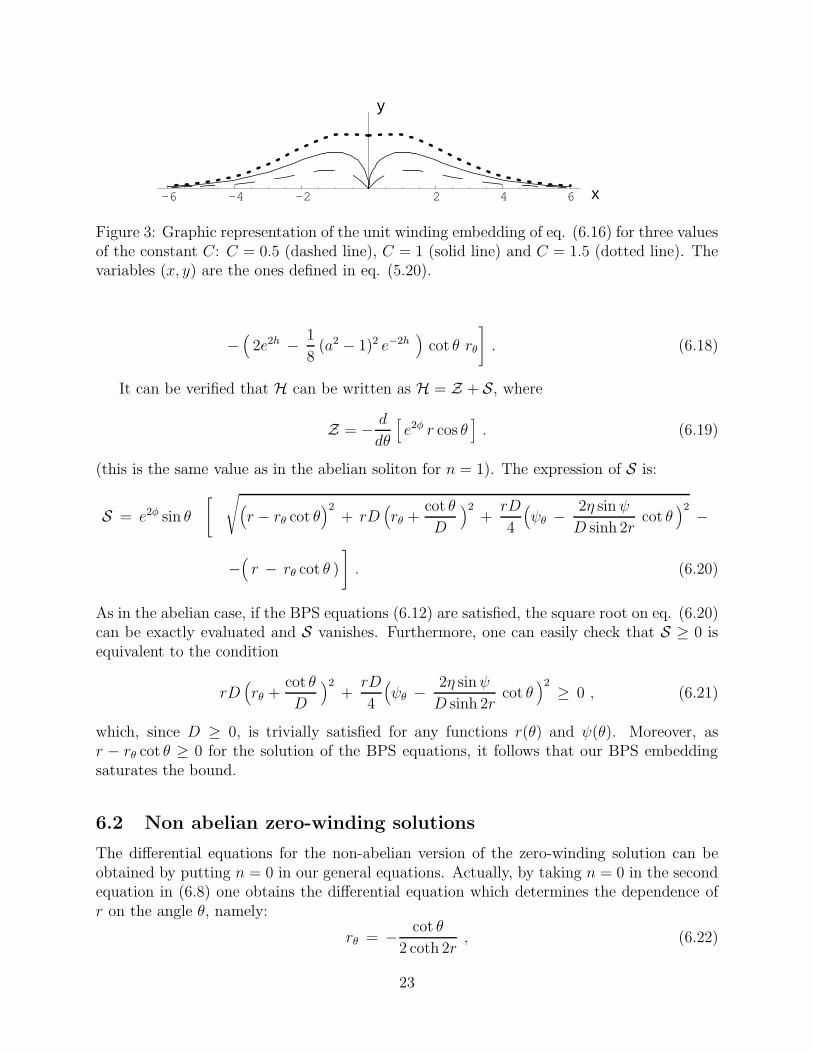
Figure 3: Graphic representation of the unit winding embedding of eq. (6.16) for three valuesof the constant C: C = 0.5 (dashed line), C = 1 (solid line) and C = 1.5 (dotted line). Thevariables (x, y) are the ones defined in eq. (5.20).

−(

2e2h − 1

8(a2 − 1)2 e−2h

)

cot θ rθ

]

. (6.18)

It can be verified that H can be written as H = Z + S, where

Z = − d

dθ

[

e2φ r cos θ]

. (6.19)

(this is the same value as in the abelian soliton for n = 1). The expression of S is:

S = e2φ sin θ

[

√

(

r − rθ cot θ)2

+ rD(

rθ +cot θ

D

)2+rD

4

(

ψθ − 2η sinψ

D sinh 2rcot θ

)2 −

−(

r − rθ cot θ )

]

. (6.20)

As in the abelian case, if the BPS equations (6.12) are satisfied, the square root on eq. (6.20)can be exactly evaluated and S vanishes. Furthermore, one can easily check that S ≥ 0 isequivalent to the condition

rD(

rθ +cot θ

D

)2+rD

4

(

ψθ − 2η sinψ

D sinh 2rcot θ

)2 ≥ 0 , (6.21)

which, since D ≥ 0, is trivially satisfied for any functions r(θ) and ψ(θ). Moreover, asr − rθ cot θ ≥ 0 for the solution of the BPS equations, it follows that our BPS embeddingsaturates the bound.

6.2 Non abelian zero-winding solutions

The differential equations for the non-abelian version of the zero-winding solution can beobtained by putting n = 0 in our general equations. Actually, by taking n = 0 in the secondequation in (6.8) one obtains the differential equation which determines the dependence ofr on the angle θ, namely:

rθ = − cot θ

2 coth 2r, (6.22)

23

which can be easily integrated, namely:

sinh 2r =C

sin θ. (6.23)

Notice that, as in the abelian case, this solution has two spikes at θ = 0, π, where r divergesand, thus, the brane probe also extends infinitely in the radial direction. Moreover, theminimal value of the radial coordinate, which we will denote by r∗, is reached at θ = π/2.This minimal value is related to the constant C in eq. (6.23), namely sinh 2r∗ = C. It isreadily verified that for large r this solution behaves exactly as the zero-winding solution inthe abelian theory. Moreover, it follows from eq. (6.4) that, in this n = 0 case, the angle ϕonly depends on θ. Actually, the differential equations for the angles θ, ϕ and ψ as functionsof θ are easily obtained from eqs. (6.6), (6.7) and (6.4):

∂θ θ = − cosψ

cosh 2r,

∂θ ϕ = − 1

cosh 2r

sinψ

sin θ,

∂θ ψ =cot θ sinψ

cosh 2r. (6.24)

By combining the equations of ψ and θ one can easily get the relation between these twoangles, namely:

sinψ =B

sin θ. (6.25)

Notice that, for consistency, B ≤ 1 and sin θ ≥ B. We can also obtain ϕ = ϕ(θ) andθ = θ(θ):

ϕ = − arctan

[

B cos θ√

sin2 θ − B2

]

+ constant ,

− arcsin

[

cos θ√1 − B2

]

= arcsin

[

cos θ√1 + C2

]

+ constant . (6.26)

Actually, much simpler equations for the embedding are obtained if one considers the par-ticular case in which the angle ψ is constant. Notice that, as was pointed out after eq. (6.8),this only can happen if ψ = 0, π (mod 2π) (see also the last equation in (6.24)). These solu-tions correspond to taking the constant B equal to zero in eq. (6.25). Moreover, it followsfrom the eq. (6.24) that ϕ is an arbitrary constant in this case, while the dependence of θ onθ can be obtained by combining eqs. (6.23) and (6.24). If we denote cosψ = ǫ, with ǫ = ±1,one has:

sinh 2r =sinh 2r∗

sin θ, sin( θ − θ∗ ) = ǫ

cos θ

cosh 2r∗, (6.27)

where θ∗ = θ(θ = π/2). Notice that there are four possible values of ψ in this zero-windingsolution and, thus, the U(1) R-symmetry is broken to ZZ 4 in this case.

24

Let us finally point out that, also in this case, the hamiltonian density H can be put asH = Z + S, where S is nonnegative (S = 0 for the BPS solution) and Z is given by:

Z = −∂θ

[

e2φ cos θ(

r − 1

4coth 2r +

r

2 sinh2 2r

)

]

. (6.28)

6.3 Cylinder solutions

We shall now show that there exists a general class of supersymmetric embeddings for thenon-abelian background. For convenience, let us consider r as worldvolume coordinate andlet us assume that the D5-brane is sitting at the north poles of the (θ, ϕ) and (θ, ϕ) two-spheres, i.e. at θ = θ = 0. In the remaining angular coordinates ϕ, ϕ and ψ, the embeddingis characterized by the equation:

ϕ− ϕ0

p=

ϕ− ϕ0

q=

ψ − ψ0

s, (6.29)

where (ϕ0, ϕ0, ψ0) and (p, q, s) are constants. Notice that, if one of the constants of thedenominator in (6.29) is zero, then the corresponding angle must be a constant. Let usparametrize these embeddings by means of two worldvolume coordinates σ1 and σ2, definedas follows:

σ1 =ϕ− ϕ0

p=

ϕ− ϕ0

q=

ψ − ψ0

s, σ2 = r . (6.30)

It is straightforward to demonstrate that the pullback to the worldvolume of the forms wi

and Ai is given by:

P [w1 ] = P [w2 ] = 0 , P [w3 ] = (q + s) dσ1 ,

P [A1 ] = P [A2 ] = 0 , P [A3 ] = −p dσ1 . (6.31)

It follows from these results that the pullback of the frame one-forms ei and ej is zero fori, j = 1, 2, whereas P [e3] is non-vanishing. As a consequence, the induced Dirac matricesare:

γσ1 =1

2(p+ q + s) e

φ

4 Γ3 , γσ2 = eφ

4 Γr . (6.32)

The kappa symmetry matrix Γκ for the embedding at hand is:

Γκ =eφ

√−g Γx0···x3 γσ1σ2 . (6.33)

Moreover, by using the projection conditions satisfied by the Killing spinors ǫ, one can provethat

γσ1σ2 ǫ = −p + q + s

2e

φ

2 Γr Γ3 ǫ =p+ q + s

2e

φ

2

(

cosαΓ12 + sinαΓ1Γ2

)

ǫ , (6.34)

25

and, since the determinant of the induced metric is√−g = e

3φ

2p+q+s

2, it is immediate to

verify that the kappa symmetry projection Γκǫ = ǫ coincides with the projection satisfiedby the Killing spinors of the background. Therefore, our brane probe preserves all thesupersymmetries of the background. Notice that the induced metric on the worldvolumealong the σ1, σ2 directions has the form

eφ

2 [(p+ q + s)2

4dσ2

1 + dσ22 ] , (6.35)

which is conformally equivalent to the metric of a cylinder. After a simple calculation onecan prove that the energy density of these solutions is

H = ∂r

[

e2φ(

pr + (q + s− p)(

coth 2r

4− r

2 sinh2 2r

))

]

. (6.36)

One can also have cylinders located at the south pole of the (θ, ϕ) and (θ, ϕ) two-spheres.Indeed, the above equations remain valid if θ = π (θ = π) if one changes p → −p (q → −q,respectively). On the other hand, if p = 0 the angle ϕ is constant and, as the pullback ofthe ei frame one-forms also vanishes when θ is also constant, it follows that θ can have anyconstant value when p = 0. Similarly, if q = 0 one necessarily has ϕ = ϕ0 and θ can be anarbitrary constant in this case.

When p = 1, q = n and s = 2m, the angular part of the embedding is the same as inthe (n,m)-winding solitons. Actually, these cylinder solutions correspond to formally takingr∗ → −∞ is the abelian solution of eq. (5.37). This forces one to take θ = 0, π and, thusone can regard the cylinder as a zoom which magnifies the region in which the probe goesto infinity. One can also get cylinder embeddings by consider the limit of the non-abeliansolutions in which the probe reaches the point r = 0. For example, by taking r∗ = 0 ineq. (6.15) one gets the p = q = 1, s = 0 cylinder solutions while the r∗ → 0 limit of theembedding (6.27) corresponds to a cylinder with p = 1 and q = s = 0. Actually, when onetakes the r∗ → 0 limit of these non-abelian embeddings one obtains two cylinder solutions,one with θ = 0 and the other with θ = π. This suggests that, in order to obtain a consistentsolution, one must combine in general two cylinders located at each of the two poles of the(θ, ϕ) two-sphere. Notice that this is also required if one imposes the condition of RR chargeneutrality of the two-sphere at infinity.

7 Quadratic fluctuations around the unit-winding em-

bedding

As mentioned in the introduction, we are now going to consider some of the brane probeconfigurations previously found as flavor branes, which will allow us to introduce dynamicalquarks in the N = 1 SYM theory. Following refs. [19, 20, 21], the spectrum of quadraticfluctuations of the brane probe will be interpreted as the meson spectrum of N = 1 SQCD.So, let us try to elaborate on the reasons to consider these probes as the addition of flavorsto the field theory dual. In fact, when considering the ’t Hooft expansion for large number of

26

colors, the role of flavors is played by the boundaries of the Feynman graph. From a gravityperspective, these boundaries correspond to the addition of D-branes and open strings in thegame.

In our case, we have a system of N D5-branes wrapping a two-cycle inside the resolvedconifold and Nf D5-branes that wrap another two-submanifold, thus introducing Nf flavorsin the SU(N) gauge theory. Taking the decoupling limit with gsα

′N fixed and large isequivalent to replacing the N D5-branes by the geometry they generate (the one studiedin section 2), while the Nf -D5 branes that do not backreact (because we take Nf muchsmaller than N) are treated as probes. From a gauge theory perspective, this is equivalentto consider the dynamics of gluons and gluinos coupled to fundamentals, but neglecting thebackreaction of the latter. Of course it would be of great interest to find the backreactedsolution.

The way of adding fundamental fields in this gauge theory from a string theory perspectivewas discussed in [28], where two possible ways, adding D9 branes or adding D5 branes asprobes, were proposed. In this paper we are considering the cleaner case of D5 probes. Acareful analysis of the open string spectrum shows the existence of a four dimensional gaugeN = 1 vector multiplet and a complex scalar multiplet. This is the spectrum of SQCD. Inthe case analyzed below we will consider abelian DBI actions for the probes, so that we willbe dealing with the Nf = 1 case.

We have found several brane configurations in the non-abelian background which, inprinciple, could be suitable to generate the meson spectrum. One of the requirements weshould demand to these configurations is that they must incorporate some scale parameterwhich could be used to generate the mass scale of the quarks. Within our framework such amass scale is nothing but the minimal distance between the flavor brane and the origin, i.e.

what we have denoted by r∗. This requirement allows to discard the cylinder solutions wehave found since they reach the origin and have no such a mass scale. We are thus left withthe unit-winding solutions of section 6.1 and the zero-winding solutions of section 6.2 as theonly analytical solutions we have found for the non-abelian background.

In this section we shall analyze the fluctuations around the unit-winding solutions of sec-tion 6.1. We have several reasons for this election. First of all, the unperturbed unit-windingembedding is simpler. Secondly, we will show in appendix B that the UV behaviour of thefluctuations is better in the unit-winding configuration than in the zero-winding embed-ding. Thirdly, the unit-winding embeddings of constant ψ incorporate the correct patternU(1) → ZZ 2 of R-symmetry breaking, whereas for the zero-winding embeddings of eq. (6.27)the U(1) symmetry is broken to a ZZ 4 subgroup.

Recall from section 6.1 that we have two possible solutions with ψ = 0, π (mod 2π),which are the ones displayed in eqs. (6.15) and (6.16). As discussed in section 6.1, thesolution of eq. (6.16) contains a one-parameter subfamily of embeddings which reach theorigin and, thus, they should correspond to massless dynamical quarks. On the contrary,the embeddings of eq. (6.15) pass through the origin only in one case, i.e. when r∗ = 0and, somehow, the limit in which the quarks are massless is uniquely defined. Recall thatfor r∗ = 0 the solution (6.15) is identical to the unit-winding cylinder. For these reasons weconsider the configuration displayed in eq. (6.15) more adequate for our purposes and wewill use it as the unperturbed flavor brane.

27

We will consider first in subsection 7.1 the fluctuations of the scalar transverse to thetransverse probe, while in subsection 7.2 we will study the fluctuations of the worldvolumegauge field. The gauge theory interpretation of the results will be discussed in subsection7.3

7.1 Scalar mesons

Let us consider a non-abelian unit-winding embedding with θ = θ, ϕ = ϕ + constant andψ = π (mod 2π). For convenience we take first r as worldvolume coordinate and consider θas a function of r, ϕ and of the unwrapped coordinates x, i.e. θ = θ(r, x, ϕ). The lagrangiandensity for such embedding can be easily obtained by computing the induced metric. Onegets:

L = −e2φ sin θ ×

×[

√

[

1 + r tanh r(

(∂rθ)2 + (∂xθ)2 +1

cos2 θ + r coth r sin2 θ(∂ϕθ)2

)

]

(r coth r + cot2 θ) +

+ r∂rθ − cot θ

]

, (7.1)

where we have neglected the term ∂r(r cos θe2φ) which, being a total radial derivative, doesnot contribute to the equations of motion.

We are going to expand this lagrangian around the corresponding non-abelian unit-winding configuration obtained in section 6.1. Actually, by taking in eq. (6.15) η = +1 oneobtains a configuration with ψ = π (mod 2π), which corresponds to a function θ = θ0(r),given by:

sin θ0(r) =sinh r∗sinh r

, (7.2)

where r∗ is the minimum value of r and r∗ ≤ r <∞. It is clear from this equation that withthe coordinate r we can only describe one-half of the brane probe: the one that is wrapped,say, on the north hemisphere of the two-sphere, in which θ ∈ (0, π/2). Outside this intervalθ0(r) is a double-valued function of r. Let us put

θ(r, x, ϕ) = θ0(r) + χ(r, x, ϕ) , (7.3)

and expand L up to quadratic order in χ. Using the first-order equation satisfied by θ0(r),namely:

∂rθ0 = − coth r tan θ0 , (7.4)

we get

L = −1

2

e2φ

1 + r coth r tan2 θ0

[

r tanh r cos θ0 (∂rχ)2 +2r

cos θ0χ ∂rχ +

r coth r

cos3 θ0χ2

]

−

− 1

2e2φ r tanh r

[

cos θ0 (∂xχ)2 +1

cos θ0 ( 1 + r coth r tan2 θ0 )(∂ϕχ)2

]

. (7.5)

28

In the equations of motion derived from this lagrangian we will perform the ansatz:

χ(r, x, ϕ) = eikx eilϕ ξ(r) , (7.6)

where, as ϕ is a periodically identified coordinate, l must be an integer and k is a four-vectorwhose square determines the four-dimensional mass M of the fluctuation mode:

M2 = −k2 . (7.7)

By substituting the functions (7.6) in the equation of motion that follows from the lagrangian(7.5), one gets a second order differential equation which is rather complicated and that canonly be solved numerically. However, it is not difficult to obtain analytically the asymptoticbehaviour of ξ(r). This has been done in appendix B and we will now use these results toexplore the nature of the fluctuations. For large r, i.e. in the UV, one gets (see eq. (B.12))that ξ(r) vanishes exponentially in the form:

ξ(r) ∼ e−r

r14

cos [√M2 − l2 r + δ ] , (r → ∞) , (7.8)

where δ is a phase and we are assuming that M2 ≥ l2. For M2 < l2 the fluctuations do notoscillate in the UV and we will not be able to impose the appropriate boundary conditions(see below). Notice that our unperturbed solution θ0(r) also decreases in the UV as

θ0(r) ∼ e−r (r → ∞) . (7.9)

Thus ξ(r)/θ0(r) → 0 as r → ∞ and the first-order expansion we are performing continues2 tobe valid in the UV. On the other hand, for r close to r∗ there are two independent solutions,one of them is finite at r = r∗ while the other diverges as

ξ(r) ∼ 1√r − r∗

. (7.10)

Let us now see how one can use the information on the asymptotic behaviour of thefluctuation modes to extract their value for the full range of the radial coordinate. First ofall, it is clear that, in principle, by consistency with the type of expansion we are adopting,one should require that ξ << θ0. Thus, one should discard the solutions which diverge in theinfrared (see, however, the discussion below). Moreover, the behaviour of the fluctuationsξ for large r should be determined by some normalizability conditions. The correspondingnorm would be an expression of the form:

∫ ∞

0dr√γ ξ2 , (7.11)

where√γ is some measure, which can be determined by looking at the lagrangian (7.5). If

we regard χ as a scalar field with the standard normalization in a curved space, then√γ is

just the coefficient of the kinetic term 12(∂rχ)2 in L, namely

√γ = e2φ r tanh r cos θ0

1 + r coth r tan2 θ0. (7.12)

2For the zero-winding solution, on the contrary, the ratio ξ(r)/θ0(r) diverges in the UV (see appendix B).

29

For large r,√γ behaves as √

γ ( r → ∞ ) ≈ r12 e2r . (7.13)

Notice that the factors on the right-hand side of eq. (7.13) cancel against the exponentialsand power factors of ξ2 in the UV (see eq. (7.8)). As a consequence, all solutions haveinfinite norm.

The reason for the bad behaviour we have just discovered is the exponential blow up ofthe dilaton in the UV which invalidates the supergravity approximation. Actually, if onewishes to push the theory to the UV one has to perform an S-duality, which basically changese2φ by e−2φ. The S-dual theory corresponds to wrapped Neveu-Schwarz fivebranes and isthe supergravity dual of a little string theory. Notice that, by changing e2φ → e−2φ in themeasure (7.12), all solutions become normalizable, which is as bad as having no normalizablesolutions at all. Moreover, it is unclear how to perform an S-duality in our D5-brane probeand convert it in a Neveu-Schwarz fivebrane for large values of the radial coordinate.

A problem similar to the one we are facing here appeared in ref. [30] in the calculationof the glueball spectrum for this background. It was argued in this reference that, in orderto have a discrete spectrum, one has to introduce a cut-off to discriminate between the tworegimes of the theory. Notice that, since they extend infinitely in the radial direction, wecannot avoid that our D5-brane probe explores the deep UV region. However, what we cando is to consider fluctuations that are significantly nonzero only on scales in which one cansafely trust the supergravity approximation. In ref. [30] it was proposed to implement thiscondition by requiring the fluctuation to vanish at some conveniently chosen UV cut-off Λ.Translated to our situation, this proposal amounts to requiring:

ξ(r)|r=Λ = 0 . (7.14)

This condition, together with the regularity of ξ(r) at r = r∗, produces a discrete spectrumwhich we shall explore below. Notice that, for consistency with the general picture describedabove, in addition to having a node at r = Λ as in eq. (7.14), the function ξ(r) should besmall for r close to the UV cut-off. This condition can be fulfilled by adjusting appropriatelythe mass scale of our solution, i.e. the minimal distance r∗ between the probe and the origin,in such a way that r∗ is not too close to Λ.

Notice that, by imposing the boundary condition (7.14) on the fluctuations, we are effec-tively introducing an infinite wall located at the UV cut-off. The introduction of this wallallows to have a discrete spectrum and should be regarded as a physical condition whichimplements the correct range of validity of the background geometry as a supergravity dualof N = 1 Yang-Mills. Even if this regularisation could appear too rude and unnatural, theresults obtained by using it for the first glueball masses are not too bad [30].

The cut-off scale Λ should not be a new scale but instead it should be obtainable fromthe background geometry itself. The proposal of ref. [30] is to take Λ as the scale ofgaugino condensation, which is believed to correspond to the point at which the functiona(r) approaches its asymptotic value a = 0. A more pragmatic point of view, to which wewill adhere here, is just taking the value of Λ which gives reasonable values for the glueballmasses. In ref. [30] the value Λ = 2 was needed to fit the glueball masses obtained fromlattice calculations, whereas with Λ = 3.5 one gets a glueball spectrum which resembles

30

0.3 1 2 3

0.5

1

ξ

r

Figure 4: Graphic representation of the first three fluctuation modes for r∗ = 0.3, Λ = 3 andl = 0. The three curves have been normalized to have ξ(r∗) = 1.

that predicted by other supergravity models. Notice that from r = 0 to r = 3 the effectivestring coupling constant eφ increases in an order of magnitude. From our point of view it isalso natural to look at the effect of the background on our brane probe. In this sense it isinteresting to point out that for r∗ = 2−3 onwards the abelian and non-abelian embeddingsare indistinguishable (see sect. 6.1).

We have performed the numerical integration of the equation of motion of ξ(r) subjectto the boundary condition (7.14) by means of the shooting technique. For a generic valueof the mass M the solution diverges at r = r∗. Only for some discrete set of masses thefluctuations are regular in the IR. In figure 4 we show the first three modes obtained by thisprocedure for r∗ = 0.3 and Λ = 3. From this figure, we notice that the number of zeroesof ξ(r) grows with the mass. In general one observes that the nth mode has n− 1 nodes inthe region r∗ < r < Λ, in agreement with the general expectation for this type of boundaryvalue problems. Moreover, for l = 0, the mass M grows linearly with the number of nodes(see below).

At this point it is interesting to pause a while and discuss the suitability of our electionof r as worldvolume coordinate. Although this coordinate is certainly very useful to extractthe asymptotic behavior of the fluctuations (specially in the UV), we should keep in mindthat we are only describing one half of the brane, i.e. the one corresponding to one of the twohemispheres of the two-sphere. On the other hand, the election of the angle as excited scalarhas some subtleties which we now discuss. Actually, to describe the displacement of thebrane probe with respect to its unperturbed configuration it is physically more sensible touse the coordinate y, defined in eq. (5.20). Accordingly, let us define the function y(r, x, ϕ)as

y(r, x, ϕ) = r sin θ(r, x, ϕ) . (7.15)

Let us put in this equation θ(r, x, ϕ) = θ0(r) + χ(r, x, ϕ). At the linear order in χ we areworking, y can be written as

y(r, x, ϕ) = y0(r) + r cos θ0(r)χ(r, x, ϕ) , (7.16)

where y0(r) ≡ r sin θ0(r) corresponds to the unperturbed brane. Notice, first of all, that forthose modes in which χ(r∗, x, ϕ) is finite, the fluctuation term in y(r∗, x, ϕ) vanishes since

31

cos θ0(r) → 0 when r → r∗. Then

y(r∗, x, ϕ) = y0(r∗) = r∗ if χ(r∗, x, ϕ) is finite . (7.17)

Thus, by considering those modes χ that are regular at r = r∗ we are effectively restrictingourselves to the modes which have a node in the y coordinate at r = r∗. If, on the contraryχ diverges for r ≈ r∗, we know from eq. (7.10) that it behaves as χ ≈ 1/

√r − r∗. But we

also know that cos θ0(r) → 0 when r → r∗ and, in fact, the second term on the right-handside of eq. (7.16) remains undetermined. The precise form in which cos θ0(r∗) vanishes canbe read from eq. (B.13), namely cos θ0(r) ≈ √

r − r∗ for r ≈ r∗. Therefore, even if χdiverges at r = r∗, we could have, in the linearized approximation we are adopting, a finitevalue for y(r∗, x, ϕ). Thus, modes with χ(r∗, x, ϕ) → ∞ should not be discarded. Actually,y(r∗, x, ϕ) − y0(r∗), although finite, is undetermined in eq. (7.16) for these modes and, inorder to obtain its allowed values we should impose a boundary condition at the other halfof the brane. As previously mentioned, this cannot be done when r is taken as worldvolumecoordinate. Therefore, it is convenient to come back to the formalism of sects. 3-5, in whichθ had been chosen as one of the worldvolume coordinates. In this approach, the unperturbedbrane configuration is described by a function r0(θ), given by:

sinh r0(θ) =sinh r∗sin θ

, (7.18)

and the brane embedding is characterized by a function r = r(θ, x, ϕ), which we expandaround r0(θ) as follows:

r(θ, x, ϕ) = r0(θ) + ρ(θ, x, ϕ) . (7.19)

Plugging this expansion into the DBI lagrangian of eq. (5.24) and keeping up to secondorder terms in ρ, one gets the following lagrangian density:

L = −1

2

e2φ sin θ r0r0 + cot2 θ tanh r0

[

coth r0 ( ∂θ ρ )2 +2 cot θ

sinh r0 cosh r0ρ∂θ ρ+

cot2 θ

sinh r0 cosh3 r0ρ2

]

−

− e2φ sin θ r02

[

(∂x ρ )2 +1

cos2 θ (1 + r0 coth r0 tan2 θ )(∂ϕ ρ )2

]

. (7.20)

Similarly to what we have done with the lagrangian (7.5), we will look for solutions of theequations of motion of L which have the form:

ρ(θ, x, ϕ) = eikx eilϕ ζ(θ) , (7.21)

where l is an integer and k2 = −M2. As before, in order to get a discrete spectrum one mustimpose some boundary conditions. In the present approach we should cutoff the regionsclose to the two poles of the two-sphere. Accordingly, let us define the following angle

sin θΛ ≡ sinh r∗sinh Λ

, θΛ ∈ (0,π

2) , (7.22)

32

-3 3

y

x

δ

Figure 5: Plot of δy ≡ ζ sin θ versus x = r cos θ for the first four modes for r∗ = 0.3, Λ = 3and l = 0. The dashed and dotted curves pass through the origin and correspond to the firsttwo modes of figure 3.

where, as indicated, we are taking θΛ in the range 0 < θΛ < π/2. Notice that θΛ → 0 ifΛ → ∞ as it should. Clearly θΛ and π− θΛ are the two angles that correspond to the radialscale Λ. Therefore, we impose the following boundary conditions to our fluctuation

ζ(θΛ) = ζ(π − θΛ) = 0 . (7.23)

The equations of motion derived from (7.20), subjected to the boundary conditions (7.23)can be integrated numerically by means of the shooting technique. One first enforces thecondition at θ = θΛ and then varies the mass M until ζ(π− θΛ) vanishes. This only happensfor a discrete set of values of the mass M . For a given value of l, let us order the solutionsin increasing value of the mass. In general one notices that the nth mode has n − 1 nodesin the interval θΛ < θ < π − θΛ and for n even (odd) the function ζ(θ) is odd (even) underθ → π− θ. In figure 5 we have plotted the first four modes corresponding to r∗ = 0.3, Λ = 3and l = 0. The modes odd under θ → π − θ vanish at θ = π/2 and their masses and shapesmatch those found with the lagrangian (7.5) and the boundary condition (7.14). On thecontrary, the modes with an even number of nodes in θΛ < θ < π − θΛ are the ones we weremissing in the formulation in which r is taken as worldvolume coordinate.

Let Mn,l(r∗,Λ) be the mass corresponding to the nth mode for a given value l and themass scales r∗ and Λ. Our numerical results are compatible with an expression of Mn,l(r∗,Λ)of the form:

Mn,l(r∗,Λ) =√

m2(r∗,Λ) n2 + l2 (7.24)

To illustrate this fact we have plotted in figure 6 the values of Mn,l(r∗,Λ) for r∗ = 0.3 andΛ = 3, together with the curves corresponding to the right-hand side of (7.24).

We have also studied the dependence of the coefficient m(r∗,Λ) on the two scales (r∗,Λ).Recall that r∗ is the minimal separation of the brane probe from the origin and, thus, canbe naturally identified with the mass of the quarks. We obtained that m(r∗,Λ) can berepresented by an expression of the type:

m(r∗,Λ) =π

2Λ+ b(Λ) r2

∗ . (7.25)

The coefficients on the right-hand side of eq. (7.25) have been obtained by a fit of m(r∗,Λ)to a quadratic expression in r∗. An example of this fit is presented in figure 7. The firstterm in eq. (7.25) is a universal term (independent of r∗) which can be regarded as a

33

2 4 6 8 10 12 14

2

4

6

8

10Mn,l

n

Figure 6: Mass spectrum for r∗ = 0.3 and Λ = 3 for l = 0, · · · , 6. The solid lines correspondto the right-hand side of eq. (7.24). The triangles (squares) are the masses of the modesζ(θ) which are even (odd) under θ → π − θ.

0.2 0.4 0.6 0.8

0.525

0.53

0.535

0.54

0.545

0.55

r*

m ( r*,Λ)

Figure 7: Dependence of m(r∗,Λ) on r∗ for Λ = 3. The solid line is a fit to the quadraticfunction (7.25).

34

finite size effect induced by our regularisation procedure. We also have determined thedependence of the coefficient b on Λ and it turns out that one can fit b(Λ) to the expressionb(Λ) = 0.23 Λ−2 + 0.53 Λ−3

We have obtained a very regular mass spectrum of particles, classified by two quantumnumbers n, l (see eqs. (7.24) and (7.25)). We can offer an interpretation of these formulas.Indeed, recall that the two-submanifold on which we are wrapping the brane is topologicallylike a cylinder, with the compact direction parametrized by the angle ϕ. The quantumnumber l is precisely the eigenvalue of the operator −i∂ϕ, which generates the shifts of ϕand, indeed, the dependence on l of the mass displayed in eq. (7.24) is the typical onefor a Kaluza-Klein reduction along a compact coordinate. Therefore, we should interpretthe mesons with l 6= 0 as composed by Kaluza-Klein modes. Moreover, the term in (7.25)proportional to r2

∗ can be understood as the contribution coming from the mass of theconstituent quarks, while the term π

2Λcan be interpreted as a contribution coming from the

‘finite size‘ of the meson. Indeed, it looks like a Casimir energy and it is originated in thepresence of the cut-off Λ.

It is perhaps convenient to emphasize again that the cut-off procedure implemented hereis a very natural procedure for this type of computations in this supergravity dual. In fact,given that the mesons are an IR effect in SQCD, we expect the contributions of high energyeffects to be irrelevant or negligible in the physical properties of the meson itself. Thisis indeed what we are doing when cutting off the integration range. We are just takinginto account the ‘non-abelian‘ part of the probes, while neglecting the ‘abelian‘ part or,equivalently, discarding high energy contributions.

7.2 Vector mesons

Let us now excite a gauge field that is living in the worldvolume of the brane. The linearizedequations of motion are:

∂m

[

e−φ √−gst Fnm]

= 0 , (7.26)

where gst is the determinant of the induced metric in the string frame and Fnm is the fieldstrength of the worldvolume gauge field Am, i.e. Fnm = ∂nAm − ∂mAn. Let us assumethat the only non-vanishing components of the gauge field A are those along the unwrappeddirections xµ of the worldvolume of the brane. In what follows we are going to use θ asworldvolume coordinate. Let us put

Aµ(θ, x, ϕ) = ǫµς(θ) eikx eilϕ , (7.27)

where ǫµ is a constant polarization four-vector and l must be an integer. It follows from theequations of motion (7.26) that ǫµ must be transverse, i.e.:

kµ ǫµ = 0 , (7.28)

and that ς(θ) must satisfy the following second-order differential equation:

∂θ

[ sin θ

tanh r0∂θ ς

]

+tanh r0sin θ

[

M2(

cos2 θ + r0 coth r0 sin2 θ)

− l2]

ς = 0 , (7.29)

35

where, as in eq. (7.7), k2 = −M2. We have solved numerically this equation by means ofthe shooting technique with the boundary conditions

ς(θΛ) = ς(π − θΛ) = 0 . (7.30)

Surprisingly, the set of possible values of M is given by the same expression as in the scalarmeson case, i.e. eq. (7.24), with a coefficient function m(r∗,Λ) which is, within the accuracyof our approximate calculation, equal numerically to that of the scalar mesons. This is quiteremarkable since the differential equations we are solving in both cases are quite different (theequation satisfied by ζ(θ) is much more complicated than eq. (7.29)). Thus, to summarize,we predict a degeneracy between the scalar and vector mesons in the corresponding N = 1SYM theory.

7.3 Gauge theory interpretation

Let us comment on some gauge theory aspects that can be read from the brane probes insections 3 to 7. For this purpose, we shall concentrate on the main solutions that havebeen used, namely, the abelian solution with unit winding (n = 1) in eq. (5.22) and itsnon-abelian extension of eq. (6.15).

First of all, let us analyze the R-symmetry of the gauge theory from the probe viewpoint.It is clear that the abelian solution (5.22) is invariant under shifts of ψ by a constant sincethe value of this angle is an arbitrary constant in this solution. This symmetry has beenidentified as the geometric dual of the R-symmetry [6, 34, 35]. Actually, this is not a U(1)invariance of the background because [6, 34, 35] of the presence of the RR form that selects,by consistency, only some particular values of the angle ψ, i.e. ψ = 2πn

Nwith 1 ≤ n ≤ 2N . So,

the abelian probes can see a ZZ 2N symmetry. In contrast, when we consider the non-abelianprobe, the solution (6.15) selects two particular values of the angle ψ, thus breaking ZZ 2N

down to ZZ 2. Notice that the U(1) → ZZ 2N breaking is an UV effect (it takes place already inthe abelian background) while the ZZ 2N → ZZ 2 breaking is an IR effect which appears onlywhen one considers the full non-abelian regular background. This same breaking pattern wasobserved in the case of SQCD with massive flavors. Indeed, as showed in [29], the theorywith massive flavors has a non-anomalous discrete ZZ 2N R-symmetry, given by (componentfields are used, λ is the gaugino and Φ and Φ are the squarks):

λ→ e−iπn/Nλ , Φ → e−iπn/NΦ , Φ → e−iπn/N Φ , (7.31)

with n = 1, ...2NAs shown in [29], this ZZ 2N symmetry is broken down to ZZ 2 by the formation of a squark

condensate. Indeed, one can see that < ΦΦ > transforms as < ΦΦ >→ e−2iπn/N < ΦΦ >leaving us with a ZZ 2. Besides, the squark condensate is consistent with supersymmetry,because the F -term equation of motion < ΦΦ > −m = 0 is satisfied. Notice that thispreservation of symmetry when m 6= 0 is in agreement with the kappa symmetry of ourbrane probes.

Apart from all this, there is a vectorial U(1) symmetry that remains unbroken in ourbrane probe analysis and that we have associated with the invariance under translations in

36

ϕ. On the field theory side this symmetry can be identified with a phase change of the fullchiral/antichiral multiplet Φ → eiαΦ, Φ → e−iαΦ, which is nothing but the U(1)B baryonicnumber symmetry of the theory. The two possible assignations ±1 of the baryonic chargeare in correspondence with the two possible identifications of the S1 described by ϕ with theS1 parametrized by ϕ. The spectrum we have found is independent of this identification.

We would like also to comment briefly on the possibility of taking the parameter r∗ = 0.Given that this parameter can be associated with the mass of the quark (since it is thecharacteristic distance between the probe brane and the background) one would like to studythe case in which this parameter is taken to be zero. Nevertheless the approach implementedhere seems to break down for this particular value of the parameter. Indeed, taking r∗ = 0will imply that θ0 = 0, so, a fluctuation of it can lead to negative values of θ taking usout of the range of this coordinate. The fact that our approach apparently does not workfor the case of massless quarks seems to be in agreement with the fact that SQCD withmassless flavors, has some special properties like spontaneous breaking of supersymmetry,the existence of a runaway potential (Affleck-Dine-Seiberg potential) and the non-existenceof a well-defined vacuum state. Notice that, when r∗ 6= 0, our approach, by construction,deals with massive quarks that preserve supersymmetry, since our probes were constructedby that requirement.

8 Summary and conclusions

Let us summarize and repeat here some points that we believe are worth stressing again.We studied a supergravity dual to N = 1 SYM, based on a geometry representing a

stack of D5 branes wrapping a two-cycle. In this gravity solution, we have found specialsurfaces where one can put probe D5-branes without spoiling supersymmetry. This wasdone, basically, by imposing that the Killing spinors of the background satisfy the projectionimposed by the kappa symmetry of the D5-brane probe.

A wide variety of kappa symmetric solutions was found and a rich mathematical struc-ture was pointed out. In fact, solutions where the probes are at a fixed distance from the”background branes” are shown to break supersymmetry. This phenomenon is in agreementwith the non-existence of moduli space of N = 1 SYM. On the other hand, we studied solu-tions corresponding to the abelian background (that is to say the large r regime of the fullbackground). These abelian solutions are shown to have a very interesting analytic structure(harmonic functions and Cauchy-Riemann equations show up) allowing interesting explicitsolutions. In extending these studies to the full background, we found several classes of non-abelian solitons. We think that it might be possible that these solutions show themselvesuseful when studying other aspects of the model not explored in this paper.

Then, in section 7, we have used the kappa symmetric solutions (in particular those thatwe called unit-winding) to introduce fundamental matter in the dual to SYM theory.

Given that the brane probes do not backreact on the background, these flavors are intro-duced in the so called quenched approximation. Nevertheless, many qualitative features andquantitative predictions for the strong coupling regime of N = 1 SQCD can be addressed.Among them, the qualitative difference between the massless and massive flavors are clear

37

in this picture. Indeed, by construction, our approach deals with the massive-flavor case,so, the problems or peculiarities of the massless case can be seen in this approach under adifferent geometrical perspective.

Other characteristic feature of SQCD with few flavors is the breaking pattern of R-symmetry. The ZZ 2N → ZZ 2 breaking is geometrically very clear from the brane probeperspective. Also, the preserved U(1)B is geometrically realized, as explained in the previoussection, by arbitrary changes in the coordinate ϕ.

A mass spectrum for the low energy excitations (mesons) of massive SQCD was foundand we believe this is a very interesting and quantitative prediction of this paper. In fact, anice formula for the masses is derived that exhibits a BPS-like behavior with the level (n)and with the Kaluza-Klein quantum number (l) of the meson. Basically, our formula givesthe meson masses in terms of the mass of the fundamentals and the Casimir energy due tofinite size of the meson, and shows explicitly the contamination of the meson spectrum dueto the Kaluza-Klein modes. It would be very interesting if lattice calculations could validateor invalidate the formula found here.

The appendices provide a hopefully very useful technical information for other workersin the area which contain, in particular, the explicit expressions of the Killing spinors of thebackground considered here and for another related background dual to N = 1 SYM theorywith a Chern-Simons term in 2 + 1 dimensions.

We believe that this paper opens some interesting routes of future research. To mentionsome of them, it should be interesting to repeat the procedure here in other “wrappedbranes” setups, dual to lower supersymmetric field theories, to see if the features for themass formula and symmetries are preserved. In particular, it would be very interesting toapply the methods employed here to the Klebanov-Strassler background [23]. The analysis ofref. [36] of the glueball spectrum suggests that, contrary to what happens to the backgroundstudied here, the spectrum of mesons could be obtained without introducing any additionalcut-off. Actually, this meson spectrum was obtained in ref. [22] from the fluctuations of aD7-brane probe wrapped on a submanifold which is analogous to our cylinders. Presumably,our method would allow us to obtain a family of supersymmetric embeddings which dependon a parameter that can be identified with the distance between the brane probe and theorigin.

On the other hand, the brane probe lagrangian should be regarded as a sort of “low energyeffective lagrangian” for the strong coupling limit of SQCD with few flavors; it would be verynice to develop the physics of this effective theory because, possibly, the scattering of mesonsand other interesting features, like low energy theorems, could be studied or understood inthis geometrical context.

Extending the treatment of this paper to non supersymmetric theories might seem acontradiction (the paper is based on kappa symmetry) but it is likely that with softly brokenbackgrounds like those appeared recently in the literature, see ref. [12], similar methods tothe ones exhibited here can be used.

38

Acknowledgments

We are grateful to D. Crooks, J. D. Edelstein, J. Erdmenger, S. A. Hartnoll, R. Hernandez,M. Kruczenski , J. M. Maldacena, D. & T. Mateos, J. Mas, J. W. Negele, L. Pando-Zayas, R.Portugues, K. Rajagopal, M. Schvellinger and D. Tong for useful discussions and encourage-ment. We have benefited of the nice atmosphere of the Benasque Center for Science, wherepart of this work has been done. C. N. is supported by a Pappalardo Fellowship, and in partby funds provided by the U.S. Department of Energy (D.O.E) under cooperative researchagreement # DF-FC02-94ER40818. A. P. and A. V. R are supported in part by MCyT,FEDER and Xunta de Galicia under grant BFM2002-03881 and by the EC Commissionunder the FP5 grant HPRN-CT-2002-00325.

A Supersymmetry of the N = 1 supergravity duals

The supersymmetry transformations for the type IIB dilatino λ and gravitino Ψµ when theRR three-form is nonzero are:

δλ =i

2∂µ φΓµ ǫ∗ +

1

24e

φ

2 F (3)µ1µ2µ3

Γµ1µ2µ3 ǫ ,

δΨµ = Dµǫ +i

96e

φ

2 F (3)µ1µ2µ3

(

Γ µ1µ2µ3µ − 9 δµ1

µ Γµ2µ3

)

ǫ∗ . (A.1)

The Killing spinors of the background are those ǫ for which the right-hand side of eq. (A.1)vanishes. In order to satisfy the equations δλ = δΨµ = 0 we will have to impose certainprojection conditions to ǫ. Once these projections are imposed, the equations δλ = δΨµ = 0are equivalent to a system of first-order differential equations for the metric and RR three-form. Moreover, following the methodology of ref. [16] (see also ref. [8]), we will be able todetermine the explicit form of ǫ from the projections that satisfies. In this appendix we willcarry out this program for two N = 1 supergravity duals which correspond to D5-braneswrapping a two- and a three-cycle.

A.1 Fivebranes wrapped on a two-cycle

For a metric ansatz such as that of eq. (2.1), let us consider the frame

exi

= eφ

4 dxi , (i = 0, 1, 2, 3) ,

e1 = eφ

4+h dθ , e2 = e

φ

4+h sin θdϕ ,

er = eφ

4 dr , ei =e

φ

4

2(wi − Ai ) , (i = 1, 2, 3) . (A.2)

39

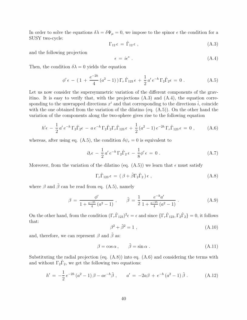
In order to solve the equations δλ = δΨµ = 0, we impose to the spinor ǫ the condition for aSUSY two-cycle:

Γ12 ǫ = Γ12 ǫ , (A.3)

and the following projectionǫ = iǫ∗ . (A.4)

Then, the condition δλ = 0 yields the equation

φ′ ǫ − ( 1 +e−2h

4(a2 − 1) ) Γr Γ123 ǫ +

1

2a′ e−h Γ2Γ2ǫ = 0 . (A.5)

Let us now consider the supersymmetric variation of the different components of the grav-itino. It is easy to verify that, with the projections (A.3) and (A.4), the equation corre-sponding to the unwrapped directions xi and that corresponding to the directions i, coincidewith the one obtained from the variation of the dilatino (eq. (A.5)). On the other hand thevariation of the components along the two-sphere gives rise to the following equation

h′ǫ − 1

2a′ e−h Γ2Γ2ǫ − a e−h Γ2Γ2ΓrΓ123 ǫ +

1

2(a2 − 1) e−2h ΓrΓ123 ǫ = 0 , (A.6)

whereas, after using eq. (A.5), the condition δψr = 0 is equivalent to

∂rǫ −1

2a′ e−h Γ2Γ2 ǫ −

1

8φ′ ǫ = 0 . (A.7)

Moreover, from the variation of the dilatino (eq. (A.5)) we learn that ǫ must satisfy

ΓrΓ123 ǫ = ( β + βΓ2Γ2 ) ǫ , (A.8)

where β and β can be read from eq. (A.5), namely

β =φ′

1 + e−2h

4(a2 − 1)

, β =1

2

e−ha′

1 + e−2h

4(a2 − 1)

. (A.9)

On the other hand, from the condition (ΓrΓ123)2ǫ = ǫ and since {ΓrΓ123,Γ2Γ2} = 0, it follows

that:β2 + β2 = 1 , (A.10)

and, therefore, we can represent β and β as:

β = cosα , β = sinα . (A.11)

Substituting the radial projection (eq. (A.8)) into eq. (A.6) and considering the terms withand without Γ2Γ2, we get the following two equations:

h′ = −1

2e−2h (a2 − 1) β − ae−hβ , a′ = −2aβ + e−h (a2 − 1) β . (A.12)

40

By using the definition of β and β (eq. (A.9)) into the second equation in (A.12), we get thefollowing relation between φ′ and a′:

φ′ = − a′

2a

[

1 − 1

4e−2h (a2 − 1)

]

. (A.13)

Furthermore, from the condition β2 + β2 = 1 one obtains a new relation between φ′ and a′,namely:

φ′2 +1

4e−2h a′2 = [ 1 +

1

4e−2h ( a2 − 1 ) ]2 . (A.14)

By combining eqs. (A.13) and (A.14) one can get the expression of φ′ and a′ in terms of aand h. Moreover, by using these results in eq. (A.9), one can get β and β as functions ofa and h and, by plugging the corresponding expressions on the first eq. in (A.12), one canobtain the differential equation for h. In order to write these expressions in a compact form,let us define:

Q ≡√

e4h +1

2e2h (a2 + 1) +

1

16(a2 − 1)2 . (A.15)

Then, one has the following system of first-order differential equations for φ, h and a:

φ′ =1

Q

[

e2h − e−2h

16(a2 − 1)2

]

,

h′ =1

2Q

[

a2 + 1 +e−2h

4(a2 − 1)2

]

,

a′ = −2a

Q

[

e2h +1

4(a2 − 1)

]

, (A.16)

and the values of β = cosα and β = sinα, which are given by:

sinα = −aeh

Q, cosα =

e2h − 14( a2 − 1 )

Q. (A.17)

It is interesting to notice that, when solving the quadratic eq. (A.14) to obtain (A.16) and(A.17), we have a sign ambiguity. We have fixed this sign by requiring that h′ is alwayspositive.

It remains to verify the fulfillment of equation (A.7). Notice first of all that the radialprojection (A.8) can be written as

Γr Γ123 ǫ = eαΓ2Γ2 ǫ , (A.18)

which, after taking into account that {ΓrΓ123,Γ2Γ2} = 0, can be solved as:

ǫ = e−α2

Γ2Γ2 ǫ0 , Γr Γ123 ǫ0 = ǫ0 . (A.19)

Inserting this parametrization of ǫ into eq. (A.7), we get two types of terms, with andwithout Γ2Γ2, which yield the following two equations:

∂rǫ0 −1

8φ′ ǫ0 = 0 , α′ = −e−h a′ . (A.20)

41

The first of these equations can be solved immediately, namely

ǫ0 = eφ

8 η , (A.21)

with η being a constant spinor. Moreover, by differentiating eq. (A.17) and using eq. (A.16),one can verify that the second equation in (A.20) is satisfied. Thus, the explicit form of theKilling spinor is

ǫ = eα2

Γ1Γ1 eφ

8 η , (A.22)

where η is a constant spinor satisfying:

Γx0···x3 Γ12 η = η , Γ12 η = Γ12 η , η = iη∗ . (A.23)

Eq. (A.16) is a system of first-order differential equations whose solution determines themetric, dilaton and RR three-form of the background. It can be verified that the valuesgiven in eq. (2.4) solve the system (A.16). Moreover, by plugging in eq. (A.15) the valuesof h and a given in eq. (2.4), one verifies that

Q = r . (A.24)

Then, one gets the following simple expression for cosα:

cosα = coth2r − 2r

sinh2 2r. (A.25)

On the other hand, being a spinor of definite chirality of type IIB supergravity, ǫ satis-fies Γx0···x3Γ12ΓrΓ123ǫ = ǫ. Thus, if we multiply the radial projection condition (A.8) byΓx0···x3Γ12, we obtain:

Γx0···x3 ( cosαΓ12 + sinαΓ1Γ2 ) ǫ = ǫ . (A.26)

Eqs. (A.3), (A.4) and (A.26) are the ones needed in the analysis of the kappa symmetry ofa D5-brane probe (eq. (2.12)).

A.2 Fivebranes wrapped on a three-cycle

As a second example of the calculation of the Killing spinors of a N = 1 supergravity dual,let us consider the supergravity solution for a D5 brane wrapped on a three-sphere. In thiscase the ansatz for the metric in Einstein frame is

ds2 = eφ

2 [ dx21,2 +

1

4R(r)2 ( σi )2 + dr2 +

1

4(wi − Ai )2 ] , (A.27)

where φ is the dilaton, R(r) is a function to be determined and σi and wi (i = 1, 2, 3) aretwo sets of su(2) left invariant one-forms. The gauge field components Ai are parametrizedin terms of a new function ω(r) as:

Ai =1 + ω(r)

2σi . (A.28)

42

Let F i be the field strength of Ai (defined as in eq. (2.6)). Its components are:

F i =ω′

2dr ∧ σi +

ω2 − 1

8ǫijk σ

j ∧ σk . (A.29)

The RR three-form of the background is now

F(3) = −1

4(w1 − A1) ∧ (w2 −A2) ∧ (w3 −A3) +

1

4

∑

i

F i ∧ (wi − Ai) + h , (A.30)

where h is determined by requiring that F(3) satisfies the Bianchi identity dF(3) = 0. Oneeasily verifies that h must satisfy the following equation

dh =1

4

∑

i

F i ∧ F i . (A.31)

By explicit calculation, one gets:

∑

i

F i ∧ F i =1

8(ω2 − 1 )ω′ ǫjkm dr ∧ σj ∧ σk ∧ σm . (A.32)

Thus, the equation for h can be solved as:

h =1

32

1

3!V (r) ǫijk σ

i ∧ σj ∧ σk , (A.33)

whereV (r) = 2ω3 − 6ω + 8k , (A.34)

with k being a constant.Let us study the supersymmetry preserved by this ansatz in the frame:

exi

= eφ

4 dxi , (i = 0, 1, 2) , er = eφ

4 dr ,

ei =1

2e

φ

4 Rσi , ei =1

2e

φ

4 (wi −Ai) , (i = 1, 2, 3) ,

(A.35)

We now impose the following projections on the spinors

Γ1Γ1 ǫ = Γ2Γ2 ǫ = Γ3Γ3 ǫ ,

ǫ = iǫ∗ . (A.36)

Then, the condition δλ = 0 becomes

φ′ ǫ −(

1 + 3ω2 − 1

4R2

)

Γr Γ123 ǫ +3ω′

4RΓ1Γ1ǫ −

V

8R3Γ1Γ1 Γr Γ123 ǫ = 0 . (A.37)

43

Moreover, from δψi = 0, one gets

R′ǫ − ω′

2Γ1Γ1ǫ +

ω2 − 1

RΓr Γ123 ǫ +

( V

8R2− ω

)

Γ1Γ1 Γr Γ123 ǫ = 0 . (A.38)

The vanishing of the supersymmetric variation of the radial component of the gravitino givesrise to:

∂rǫ −3ω′

4RΓ1Γ1ǫ −

1

8φ′ ǫ = 0 , (A.39)

where we have used eq. (A.37). Let us solve these equations by taking the projection

Γr Γ123 ǫ = ( β + βΓ1Γ1 ) ǫ . (A.40)

As in case studied in section (A.1), from (Γr Γ123)2 ǫ = ǫ and {Γr Γ123,Γ1Γ1} = 0 it follows

that β2 + β2 = 1 and thus we can take β = cosα and β = sinα.Let us substitute our ansatz for Γr Γ123 ǫ (eq. (A.40)) on the equations coming from the

dilatino and gravitino (eqs. (A.37) and (A.38)). From the terms containing the unit matrix,we obtain equations for φ′ and R′:

φ′ =(

1 + 3ω2 − 1

4R2

)

β − V

8R3β ,

R′ =1 − ω2

Rβ +

( V

8R2− ω

)

β . (A.41)

Moreover, by considering the terms with Γ1Γ1, we obtain two expressions for ω′

3ω′ =V

2R2β +

(

4R + 3ω2 − 1

R

)

β ,

ω′ =( V

4R2− 2ω

)

β + 2ω2 − 1

Rβ . (A.42)

By combining these last two equations we get

( V

24R2− w

)

β =( 1 − w2

2R+

2R

3

)

β . (A.43)

By plugging this last relation in the condition β2 + β2 = 1 one can easily obtain theexpression of β and β. Indeed, let us define M as follows:

M ≡( V

24R2− w

)2+( 1 − w2

2R+

2R

3

)2. (A.44)

In terms of this new quantity M , the coefficients β and β are given by:

β = cosα =1√M

(

2R

3+

1 − ω2

2R

)

, β = sinα =1√M

(

V

24R2− ω

)

. (A.45)

44

By using these values of β and β in the equations which determine R ′, ω ′ and φ′, we obtaina system of first-order BPS equations which are identical to those written in refs. [31, 32, 33](see also ref. [37]). They are:

R ′ =1

3√M

[ V 2

64R4+

1

2R2

(

3(1 − ω2)2 − V ω)

+ ω2 + 2]

,

ω ′ =4R

3√M

[ V

32R4( 1 − ω2 ) +

2k − ω3

2R2− ω

]

,

φ′ = −3

2( logR )′ +

3

2

√M

R. (A.46)

The radial projection condition (A.40) can be written as

Γr Γ123 ǫ = eαΓ1Γ1 ǫ . (A.47)

Since {Γr Γ123,Γ1Γ1} = 0, this equation can be solved as:

ǫ = e−α2

Γ1Γ1 ǫ0 , Γr Γ123 ǫ0 = ǫ0 . (A.48)

Plugging now this parametrization of ǫ into the equation obtained from the variation of theradial component of the gravitino (eq. (A.39) ), we arrive at the following two equations:

∂r ǫ0 =φ′

8ǫ0 , α′ = −3

2ω′R . (A.49)

The equation for ǫ0 can be solved immediately:

ǫ0 = eφ

8 η , (A.50)

where η is a constant spinor. Moreover, one can verify that the equation for α is a consequenceof the first-order BPS equations (A.46). Therefore, the Killing spinors for this geometry areof the form:

ǫ = e−α2

Γ1Γ1 eφ

8 η , (A.51)

where η is constant and satisfies the following conditions:

Γx0···x2 Γ123 η = η ,

Γ1Γ1 η = Γ2Γ2 η = Γ3Γ3 η ,

η = iη∗ . (A.52)

Notice that, for the spinor ǫ, the first of these projections can be recast in the form:

Γx0···x2

(

cos αΓ123 − sinαΓ123

)

ǫ = ǫ . (A.53)

45

B Asymptotic behaviour of the fluctuations

This appendix is devoted to the determination of the asymptotic form of the fluctuationsaround the kappa-symmetric static configurations of the D5-brane probe. In subsection B.1we will consider the large and small r behaviour of the solutions of the equation of motioncorresponding to the lagrangian (7.5), which describes the small oscillations around the unit-winding embedding (7.2). In section B.2 we will study the asymptotic form of the fluctuationsof the n-winding embedding in the abelian background. Following our general arguments,the UV behaviour of the abelian and non-abelian fluctuations must be the same and, thus,from this analysis we can get an idea of the nature of the small oscillations around the generalnon-abelian n-winding configurations (whose analytical form we have not determined) forlarge values of the radial coordinate.

B.1 Non abelian unit-winding embedding

For large r the lagrangian (7.5) takes the form:

L = −1

2e2φ [ r (∂rχ)2 + 2r χ ∂rχ + rχ2 + r (∂xχ)2 + r (∂ϕχ)2 ] , (B.1)

where we have not expanded the dilaton and we have eliminated the exponentially suppressedterms. Using the asymptotic value of ∂rφ:

∂rφ ≈ 1 − 1

4r − 1, (B.2)

we obtain the following equation for ξ:

∂2r ξ +

8r2 − 1

4r2 − r∂r ξ +

(

M2 − l2 + 1 +2r − 1

4r2 − r

)

ξ = 0 . (B.3)

To study the UV behaviour of the solutions of this differential equation it is interesting torewrite it with the different coefficient functions expanded in powers of 1/r as:

∂2r ξ + ( a0 +

a1

r+a2

r2+ · · · ) ∂r ξ + ( b0 +

b1r

+b2r2

+ · · · ) ξ = 0 , (B.4)

where

a0 = 2 , b0 = M2 − l2 + 1 , a1 = b1 =1

2, a2 = b2 = −1

8, · · · (B.5)

We want to solve eq. (B.4) by means of an asymptotic Frobenius expansion of the typeξ = rρ (c0 + c1/r + · · ·) for some exponent ρ. By substituting this expansion on the right-hand side of eq. (B.4) and comparing the terms with the different powers of r, we noticethat there is only one term with rρ, namely b0c0r

ρ, which cannot be canceled. In order toget rid of this term, let us define a new function w as

ξ = eαr w , (B.6)

46

with α being a number to be determined. The equation satisfied by w is the same as thatof ξ with the changes:

a0 → a0 + 2α , b0 → α2 + αa0 + b0 ,

ai → ai , bi → bi + αai , (i = 1, 2, · · ·) . (B.7)

It is clear that we must impose the condition:

α2 + αa0 + b0 = 0 , (B.8)

which determines the values of α. Writing now w = rρ (c0 + c1/r + · · ·) and looking at thehighest power of r in the equation of w (i.e. ρ − 1), we immediately obtain the value of ρ,namely:

ρ = −αa1 + b12α + a0

, (B.9)

and, clearly, as r → ∞ the asymptotic behaviour of ξ(r) is:

ξ(r) ≈ eαr rρ ( 1 + o(1

r) ) . (B.10)

In our case, it is easy to verify that the values of α and ρ are:

α = −1 ± i√M2 − l2 , ρ = −1

4. (B.11)

Then, it is clear that we have two independent behaviours for the real function ξ(r), namely:

ξ(r) ∼ e−r

r14

cos(√

M2 − l2 r)

,e−r

r14

sin(√

M2 − l2 r)

. (B.12)

Notice that all solutions decrease exponentially when r → ∞.Let us now turn to the analysis of the fluctuations for small values of the radial coordinate.

Recall that r∗ ≤ r ≤ ∞. Near r∗, one can expand sin θ0 and cos θ0 as follows:

sin θ0 ≈ 1 − coth r∗ (r − r∗) +1

2

1 + cosh2 r∗

sinh2 r∗(r − r∗)

2 + · · · ,

cos θ0 ≈√

2 coth r∗(r − r∗)[

1 − coth r∗2

(1 +1

2 cosh2 r∗) (r − r∗) + · · ·

]

. (B.13)

Using these expressions it is straightforward to show that the lagrangian density of thequadratic fluctuations is given by:

L = −1

2e2φ∗ [A(r) ( ∂rχ)2 +B(r)2χ∂rχ+ C(r)χ2 +D(r) ( ∂xχ)2 + E(r) ( ∂ϕχ)2 ] , (B.14)

47

where φ∗ = φ(r∗) and the functions A,B,C,D and E are of the form:

A(r) = [ 8 tanh r∗ (r − r∗)3 ]

12 ( 1 + A(r) ) ,

B(r) =

√

2(r − r∗)√coth r∗

( 1 + B(r) ) ,

C(r) =1

√

2 coth r∗ (r − r∗)( 1 + C(r) ) ,

D(r) =r∗√

coth r∗

√

2(r − r∗) ( 1 + D(r) ) ,

E(r) = [ tanh r∗ ]32

√

2(r − r∗) ( 1 + E(r) ) . (B.15)

The functions A,B, C,D, E , satisfy:

A(r),B(r), C(r),D(r) E(r) ∼ o(r − r∗) . (B.16)

Notice that, remarkably, after integrating by parts the χ∂rχ term in the lagrangian, thesingular term of C(r) cancels against the leading term of B(r). The equation of motion forξ near r∗ is:

∂2r ξ +

A′(r)

A(r)∂rξ +

B′(r) − C(r) +M2D(r) − l2E(r)

A(r)ξ = 0 . (B.17)

In order to solve this equation in a power series expansion in r − r∗, it is important tounderstand the singularities of the different coefficients near r∗. It is immediate that:

A′(r)

A(r)=

3

2

1

r − r∗+

A′(r)

1 + A(r)=

3

2

1

r − r∗+ regular . (B.18)

Similarly, the coefficient of ξ has a simple pole near r∗:

B′(r) − C(r) +M2D(r) − l2E(r)

A(r)=

3B ′(r∗) − C ′(r∗) + 2M2r∗ − 2l2 tanh r∗4

1

r − r∗+ regular .

(B.19)

It follows that the point r = r∗ is a singular regular point. The corresponding Frobeniusexpansion reads:

ξ(r) = (r − r∗)λ

∞∑

n=0

cn (r − r∗)n , (B.20)

where λ satisfies the indicial equation, which can be obtained by plugging the expansion inthe equation and looking at the term with lowest power of r− r∗ (i.e. λ− 2). In our case, λmust be a root of the quadratic equation:

λ(λ− 1) +3

2λ = 0 , (B.21)

48

i.e.:

λ = 0,−1

2. (B.22)

This means that there are two independent solutions of the differential equation which canbe represented by a Frobenius series around r = r∗, one of then is regular as r → r∗ (the one

corresponding to λ = 0), whereas the other diverges as (r − r∗)− 1

2 .

B.2 n-Winding embeddings in the abelian background

Let us consider the abelian background and an embedding with winding number n, for which∂ϕϕ = n, sin θ∂θ θ = n sin θ and ψ = ψ0 = constant. Let us define

V ≡ n

2

cos θ

sin θ+

1

2cot θ =

n

2 sin θ

(1 + cos θ)n − (1 − cos θ)n

(1 + cos θ)n + (1 − cos θ)n+

1

2cot θ ,

W ≡ n

2

sin θ

sin θ=

n(sin θ)(n−1)

(1 + cos θ)n + (1 − cos θ)n. (B.23)

Choosing r as worldvolume coordinate and considering embeddings in which θ depends onboth r and on the unwrapped coordinates x, we obtain the following lagrangian:

L = −e2φ sin θ

[

√

( e2h + V 2 + W 2 ) ( 1 + (e2h + W 2)((∂rθ)2 + (∂xθ)2))+

+ (e2h + W 2)∂rθ − V

]

. (B.24)

We shall expand this lagrangian around a configuration θ0(r) such that

e2(r−r∗) =1

2

(1 + cos θ0(r))n + (1 − cos θ0(r))

n

(sin θ0(r))n+1. (B.25)

Notice that θ0(r) remains unchanged under the transformation n→ −n. Thus, without lossof generality we shall restrict ourselves from now on to the case n ≥ 0. Let us now define

V0(r) ≡ V |θ(r)=θ0(r) , W0(r) ≡ W |θ(r)=θ0(r) , V0θ(r) ≡∂V

∂θ

∣

∣

∣

θ(r)=θ0(r). (B.26)

Using

∂rθ0 = − 1

V0

, (B.27)

we obtain the following quadratic lagrangian

L = −e2φ

2sin θ0 (e2h + W 2

0 )

[

1

e2h + V 20 + W 2

0

(

V 30 (∂rχ)2 − 2V0 V0θ χ∂rχ +

+V 2

0θ

V0χ2)

+ V0 (∂xχ)2

]

. (B.28)

49

Keeping the leading terms for large r, the lagrangian becomes:

L = −r2e2φ [

n + 1

2(∂rχ)2 + 2χ∂rχ +

2

n+ 1χ2 +

n + 1

2(∂xχ)2 ] , (B.29)

and, if we represent χ as in eq. (7.6) with l = 0, the equation of motion for ξ becomes:

∂2r ξ + (2 +

1

2r) ∂rξ +

(

M2 +4n

(n+ 1)2+

1

n+ 1

1

r

)

ξ = 0 . (B.30)

Now we have the following coefficients in eq. (B.4):

a0 = 2 , b0 = M2 +4n

(n+ 1)2, a1 =

1

2, b1 =

1

n+ 1. (B.31)

By plugging these values in eq. (B.8) we obtain the following result for the coefficient α ofthe exponential:

α = −1 ±√

(n− 1

n+ 1

)2 − M2 . (B.32)

Let us distinguish two cases, depending on the sign inside the square root. Suppose firstthat M2 ≥ (n−1

n+1)2 and define

M2 = M2 −(n− 1

n+ 1

)2. (B.33)

In this case the values of the exponent ρ obtained from (B.9) are:

ρ = −1

4∓ n− 1

2(n+ 1)Mi . (B.34)

It follows that the two real asymptotic solutions are:

ξ(r) ∼ e−r

r14

cos [Mr − n− 1

2(n+ 1)Mlog r] ,

e−r

r14

sin [Mr − n− 1

2(n+ 1)Mlog r] . (B.35)

Both solutions vanish exponentially when r → ∞.If M2 < 0, let us define M2 = −M2. In this case α is real, namely α = −1 ± M . Notice

that M < 1 and thus α < 0. The independent asymptotic solutions are:

ξ(r) ∼ e(M−1)r r− 1

4(1− n−1

(n+1)M), e−(M+1)r r

− 14(1+ n−1

(n+1)M), (B.36)

and both decrease exponentially, without oscillations, when r → ∞. This non-oscillatorycharacter of the functions in eq. (B.35) make them inadequate for the type of boundaryconditions we are imposing and, therefore, we shall discard them.

Notice that, for n = 1, the large r asymptotic solutions (B.12) and (B.35) coincide.This is of course to be expected since the abelian and non-abelian configurations coincide inthe UV. It is also interesting to compare the magnitude of the fluctuation with that of theunperturbed configuration for large r. By inspecting eq. (B.25) one readily concludes that

θ0(r) ∼ e−2

n+1r , (r → ∞) . (B.37)

50

By comparing this behaviour with eq. (B.35) one finds

ξ(r)

θ0(r)∼ e−

n−1n+1

r

r14

, (r → ∞) . (B.38)

Thus, for n ≥ 1 one has that ξ(r)θ0(r)

→ 0 as r → ∞. On the contrary for n = 0, both in the

abelian and non-abelian case, the ratio ξ(r)θ0(r)

diverges in the UV and the first order expansionbreaks down.

Let us now consider the IR behaviour of the fluctuations. Near r∗ one has to leadingorder that sin θ0 ≈ 1 and

cos θ0 ≈2√

1 + n2

√r − r∗ , V0 ≈

√n2 + 1

√r − r∗ ,

W0 ≈n

2, V0θ ≈ −n

2 + 1

2. (B.39)

The IR lagrangian is of the same form as in eq. (B.14) (with E = 0 since we are nowconsidering the case in which χ is independent of ϕ). The functions A(r) to D(r) are nowof the form

A(r) =[

(n2 + 1)(r − r∗)] 3

2(

1 + o(r − r∗))

,

B(r) =(n2 + 1)

32

2

√r − r∗

(

1 + o(r − r∗))

,

C(r) =1

4

(n2 + 1)32√

r − r∗

(

1 + o(r − r∗))

,

D(r) =(

r∗ +n2 − 1

4

)√n2 + 1

√r − r∗

(

1 + o(r − r∗))

. (B.40)

Notice that, also in this case, the coefficients of the functions above are such that, after apartial integration, the singular term of C(r) cancels against the leading term of B(r). Thedifferential equation that follows for ξ in the IR is:

∂2r ξ +

(3

2

1

r − r∗+ o(r − r∗)

)

∂rξ + o(1

r − r∗) ξ = 0 , (B.41)

and, therefore, the indicial equation is the same as for eq. (B.17) (i.e. eq. (B.21)). It followsthat also in this case there exists an independent solution which does not diverge whenr → r∗.

References

[1] G. ’t Hooft, “A planar diagram theory for strong interactions”, Nucl. Phys. B72 (1974)461.

51

[2] J. M. Maldacena, “The large N limit of superconformal field theories and supergravity”,Adv. Theor. Math. Phys. 2 (1998) 231, hep-th/9711200.

[3] O. Aharony, S. Gubser, J. Maldacena, H. Ooguri and Y. Oz, “Large N field theories,string theory and gravity”, Phys. Rept. 323 (2000) 183, hep-th/9905111.

[4] J. M. Maldacena and C. Nunez, “Supergravity description of field theories on curvedmanifolds and a no go theorem”, Int. J. Mod. Phys. A16 (2001) 822, hep-th/0007018.

[5] M. Bershadsky, C. Vafa and V. Sadov, “D-Branes and Topological Field Theories”,Nucl. Phys. B463 (1996) 420, hep-th/9511222.

[6] J. M. Maldacena and C. Nunez, “Towards the large N limit of pure N = 1 super YangMills, Phys. Rev. Lett. 86 (2001) 588, hep-th/0008001.

[7] A. H. Chamseddine and M. S. Volkov, “Non-Abelian BPS monopoles in N = 4 gaugedsupergravity, Phys. Rev. Lett. 79 (1997) 3343, hep-th/9707176; “Non-Abelian solitonsin N = 4 gauged supergravity and leading order string theory”, Phys. Rev. D57 (1998)6242, hep-th/9711181.

[8] R. Apreda, F. Bigazzi, A. L. Cotrone, M. Petrini and A. Zaffaroni, “Some commentson N=1 gauge theories from wrapped branes”, Phys. Lett. B536 (2002) 161, hep-th/0112236.

[9] P. Di Vecchia, A. Lerda and P. Merlatti, “N=1 and N=2 super Yang-Mills theories fromwrapped branes”, Nucl. Phys. B646 (2002) 43, hep-th/0205204.

[10] M. Bertolini and P. Merlatti, “A note on the dual of N = 1 super Yang-Mills theory”,Phys. Lett. B556 (2003) 80, hep-th/0211142.

[11] P. Merlatti, ”N=1 super Yang-Mills theories and wrapped branes”, Class. Quant. Grav.

20 (2003)S541, hep-th/0212203.

[12] G. Papadopoulos and A. A. Tseytlin, “Complex geometry of conifolds and 5-branewrapped on 2-sphere”, Class. Quant. Grav. 18 (2001)1333, hep-th/0012034;A. Loewy and J. Sonnenschein, “On the holographic duals of N = 1 gauge dynamics”,J. High Energy Phys. 0108 (2001) 007, hep-th/0103163;S. S. Gubser, A. A. Tseytlin and M. S. Volkov, “Non-abelian 4-d black holes, wrapped5-branes and their dual descriptions”, J. High Energy Phys. 0109 (2001) 017, hep-th/0108205;O. Aharony, E. Schreiber and J. Sonnenschein, “Stable non-supersymmetric supergrav-ity solutions from deformations of the Maldacena-Nunez background”, J. High Energy

Phys. 0204 (2002) 011, hep-th/0201224;N. Evans, M. Petrini and A. Zaffaroni, “The gravity dual of softly broken N = 1 superYang-Mills”, J. High Energy Phys. 0206 (2002) 004, hep-th/0203203;T. Mateos, J. M. Pons and P. Talavera, “Supergravity dual of noncommutative N=1SYM”, Nucl. Phys. B651 (2003) 291, hep-th/0209150;

52

X.-J. Wang and S. Hu, “Green functions of N = 1 SYM and radial/energy-scale rela-tion”, Phys. Rev. D67 (2003) 105012, hep-th/0210041;W. Muck, “Perturbative and non-perturbative aspects of pure N = 1 super Yang-Millstheory from wrapped branes”, J. High Energy Phys. 0302 (2003) 013, hep-th/0301171;R. Apreda, “Non supersymmetric solutions from wrapped and fractional branes”, hep-th/0301118.

[13] M. Bertolini, “Four lectures on the gauge/gravity correspondence”, hep-th/0303160;F. Bigazzi, A. L. Cotrone, M. Petrini and A. Zaffaroni, “Supergravity duals of super-symmetric four dimensional gauge theories”, Riv. Nouvo Cim. 25N12 (2002)1, hep-th/0303191.

[14] M. Cederwall, A. von Gussich, B.E.W. Nilsson, P. Sundell and A. Westerberg, The

Dirichlet super-p-branes in Type IIA and IIB supergravity, Nucl. Phys. B490 (1997)179, hep-th/9611159:E. Bergshoeff and P.K. Townsend, Super D-branes Nucl. Phys. B490 (1997) 145, hep-th/9611173;M. Aganagic, C. Popescu and J.H. Schwarz, D-brane actions with local kappa symmetry,Phys. Lett. B393 (1997) 311, hep-th/9610249; Gauge-invariant and gauge-fixed D-brane

actions, Nucl. Phys. B495 (1997) 99, hep-th/9612080.

[15] K. Becker, M. Becker and A. Strominger, Fivebranes, membranes and non-perturbative

string theory, Nucl. Phys. B456 (1995) 130, hep-th/9507158;E. Bergshoeff, R. Kallosh, T. Ortin and G. Papadopulos, κ-symmetry, supersymmetry

and intersecting branes, Nucl. Phys. B502 (1997) 149, hep-th/9705040;E. Bergshoeff and P.K. Townsend, Solitons on the supermembrane, J. High Energy

Phys. 9905 (1999) 021, hep-th/9904020.

[16] J. D. Edelstein, A. Paredes and A. V. Ramallo, “Let’s twist again: general metrics ofG2 holonomy from gauged supergravity”, J. High Energy Phys. 0103 (2003) 011, hep-th/0211203; “Singularity resolution in gauged supergravity and conifold unification”,Phys. Lett. B554 (2003) 197, hep-th/0212139.

[17] J.D. Edelstein and C. Nunez, “D6 branes and M-theory geometrical transitions fromgauged supergravity”, J. High Energy Phys. 0104, (2001) 028, hep-th/0103167;R. Hernandez and K. Sfetsos, “An eight-dimensional approach to G(2) manifolds”, Phys.

Lett. B536. (2002) 294, hep-th/0202135.

[18] J.P. Gauntlett, J. Gomis and P.K. Townsend, BPS bounds for worldvolume branes, J.

High Energy Phys. 9801 (1998) 003, hep-th/9711205.

[19] A. Karch and E. Katz, “Adding flavor to AdS/CFT”, J. High Energy Phys. 0206 (2002)043, hep-th/0205236.

[20] A. Karch, E. Katz and N. Weiner, “Hadron masses and screening from AdS Wilsonloops”, Phys. Rev. Lett. 90 (2003) 091601, hep-th/0211107.

53

[21] M. Kruczenski, D. Mateos, R. Myers and D. Winters, “Meson spectroscopy in AdS/CFTwith flavour”, J. High Energy Phys. 0307 (2003) 049, hep-th/0304032.

[22] T. Sakai and J. Sonnenschein, “Probing flavored mesons of confining gauge theories bysupergravity”, J. High Energy Phys. 0309 (2003) 047, hep-th/0305049.

[23] I. R. Klebanov and M. J. Strassler, “Supergravity and a confining gauge theory: dualitycascades and a chiSB-resolution of naked singularities”, J. High Energy Phys. 0008(2000) 052, hep-th/0007191.

[24] J. Babington, J. Erdmenger, N. Evans, Z. Guralnik and I. Kirsch, “Chiral symmetrybreaking and pions in non-supersymmetric gauge/gravity duals”, hep-th/0306018.

[25] M. Kruczenski, D. Mateos, R. Myers and D. Winters, ‘Towards a holographic dual oflarge-Nc QCD”, hep-th/0311270.

[26] E. Imeroni and A. Lerda, “Non-perturbative gauge superpotentials from supergravity”,hep-th/0310157.

[27] P. Ouyang, “Holomorphic D7-branes and flavored N=1 gauge dynamics”, hep-th/0311084.

[28] X.-J. Wang and S. Hu, “Intersecting branes and adding flavors to the Maldacena-Nunezbackground”, J. High Energy Phys. 0309 (2003) 017, hep-th/0307218.

[29] I. Affleck, M. Dine and N. Seiberg, “Dynamical Supersymmetry Breaking In Supersym-metric QCD” Nucl. Phys. B241, 493 (1984).

[30] L. Ametller, J. M. Pons and P. Talavera, “On the consistency of the N = 1 SYM spectrafrom wrapped five branes”, hep-th/0305075.

[31] M. Schvellinger and T. A. Tran, “Supergravity duals of gauge field theories from SU(2)×U(1) gauged supergravity in five dimensions”, J. High Energy Phys. 0106 (2001) 025,hep-th/0105019.

[32] J. Maldacena and H. Nastase, “The supergravity dual of a theory with dynamical su-persymmetry breaking”, J. High Energy Phys. 0109 (2001) 024, hep-th/0105049.

[33] A. H. Chamseddine and M. S. Volkov, “Non-abelian vacua in D=5, N=4 gauged super-gravity, J. High Energy Phys. 0104 (2001) 023, hep-th/0101202.

[34] I. R. Klebanov, P. Ouyang and E. Witten, “A gravity dual of the chiral anomaly”, Phys.

Rev. D65, 105007 (2002), hep-th/0202056.

[35] U. Gursoy, S. A. Hartnoll and R. Portugues, “The chiral anomaly from M-theory”,hep-th/0311088.

[36] M. Krasnitz, “A two point function in a cascading N=1 gauge theory from supergrav-ity, hep-th/0011179; E. Caceres and R. Hernandez, “Glueball masses for the deformedconifold theory”, Phys. Lett. B504 (2001) 64, hep-th/0011204.

54

[37] J. Gomis, “On Susy breaking and χSB from string duals”, Nucl. Phys. B624 (2002)181, hep-th/0111060.

55