arX

iv:0

904.

4033

v2 [

hep-

lat]

29

Sep

2009

Landau-gauge propagators in Yang-Mills theories at β = 0:

massive solution versus conformal scaling

A. Cucchieri1 and T. Mendes1, 2

1Instituto de Fısica de Sao Carlos, Universidade de Sao Paulo,Caixa Postal 369, 13560-970 Sao Carlos, SP, Brazil

2DESY–Zeuthen, Platanenallee 6, 15738 Zeuthen, Germany(Dated: February 19, 2013)

We study Landau-gauge gluon and ghost propagators in Yang-Mills theories at lattice parameterβ = 0, considering relatively large lattice volumes for the case of the SU(2) gauge group in three andfour space-time dimensions. We compare the lattice data to the so-called massive and conformal-scaling solutions, examining the requirements for a good description of the propagators over variousranges of momenta and discussing possible systematic errors. Our analysis strongly supports themassive solution, i.e. a finite gluon propagator and an essentially free ghost propagator in the infraredlimit, in disagreement with Ref. [1]. Moreover, we argue that discretization effects play no role inthe analysis of these propagators.

PACS numbers: 11.10.Kk 11.15.Ha 12.38.Aw 12.38.Gc 14.70Dj

I. INTRODUCTION

In recent years, considerable effort has been invested inthe study of the infrared (IR) behavior of Green’s func-tions in Yang-Mills theories. The results of these stud-ies, using analytic methods as well as numerical latticesimulations, are usually compared to the predictions ofvarious confinement scenarios. Since Green’s functionsare gauge-dependent quantities, one can expect to finddifferent confinement pictures when considering differentchoices of the gauge.

Here we consider the Landau gauge and test the pre-dictions of the Gribov-Zwanziger and Kugo-Ojima con-finement scenarios at lattice parameter β = 0, i.e. inthe limit of infinite lattice coupling. This study is verysimilar to that presented in Refs. [1, 2, 3]. On the otherhand, it is not intended to be a simple duplication of thatwork since, in particular, the analysis we present here isnot done exactly in the same way as in Ref. [1]. Also,even though there is probably no real difference at thelevel of the lattice data, as we show in Section II C andexplain in Sections I E and III, we mostly do not agreewith the data analysis and the interpretation of the re-sults presented in Ref. [1]. The interested reader is ofcourse invited to read both papers and form her/his ownopinion on this subject.

A. Confinement scenarios in Landau gauge

In Landau gauge, the Gribov-Zwanziger scenario [4,5, 6, 7] relates confinement of quarks to a ghost propa-gator G(p) enhanced in the IR limit when compared tothe tree-level behavior 1/p2 as a function of the momen-tum p. Indeed, in this scenario, the enhancement of G(p)should account for the long-range mechanism responsiblefor confinement. An enhanced ghost propagator is alsoobtained by the Kugo-Ojima color-confinement criterion

[8, 9]. Consequently, in both cases one expects to findlimp→0 p2G(p) = ∞, which is referred to as ghost domi-

nance [10, 11].

At the same time, the gluons should be confined dueto the violation of reflection positivity [12]. This impliesthat the gluon propagator in position space D(x) shouldbe negative for a range of values of the space-time sepa-ration x. Since the gluon propagator at zero momentumD(p = 0) is proportional to

∫

ddxD(x), it is clear thatnegative values for D(x) will tend to reduce the value ofD(p = 0), leading to a suppression of D(p) at small mo-menta [4, 12, 13]. Similarly, in the Kugo-Ojima scenarioone can show that the perturbative massless pole of thegluon propagator probably disappears as a consequenceof the confining criterion [9]. Thus, an IR-suppressedgluon propagator can also be accommodated in the Kugo-Ojima confinement scenario [10]. Clearly, maximal vio-lation of reflection positivity is obtained if D(p = 0) = 0.

Even though these two scenarios predict similar behav-iors for the gluon and ghost propagators in Landau gauge,one should recall that the line of thinking in the two casesis quite different. Indeed, in the Gribov-Zwanziger sce-nario confinement is due to the properties of the config-urations belonging to the boundary of the so-called firstGribov region [4, 5, 7], which should be the relevant con-figurations in Landau gauge. On the contrary, in theKugo-Ojima scenario [8, 9], confinement is obtained ifone can define unbroken global color charges. Moreover,in the latter case, Gribov copies do not seem to playany role in the confining mechanism. Nevertheless, if oneuses the Kugo-Ojima confinement criterion as a boundarycondition [14] then the partition function is equivalent tothe one obtained using the Gribov-Zwanziger approach,i.e. by restricting the functional integration to the firstGribov region.

2

B. Massive and conformal-scaling solutions

Yang-Mills theories can be studied non-perturbativelyusing the field equations of motion of the theory, i.e. thesets of coupled Dyson-Schwinger equations (DSE) [15].Usually, the solution of these equations depends on theconsidered truncation scheme and on the approximationsemployed.

Recently, it has been shown [16, 17] that there exist twopossible consistent solutions of the DSE in 4d Landaugauge. One solution, usually called conformal scaling,gives an IR-enhanced ghost propagator G(p) ∼ p−2(1+κG)

and an IR-finite gluon propagator D(p) ∼ p2(2κZ−1) withinfrared exponents κG = κZ ≡ κ ∈ [1/2, 3/4]. Notethat D(0) = 0 for κ > 1/2. The second solution, calledmassive or decoupling solution, is characterized by a tree-level-like ghost propagator at small momenta G(p) ∼ p−2

and by a finite nonzero gluon propagator D(0) > 0 atzero momentum (i.e., κG = 0, κZ = 1/2).

These two solutions have indeed been obtained by sev-eral groups [18, 19, 20, 21, 22, 23, 24], using differenttruncation schemes. Let us recall that the conformal so-lution has also been obtained (in Landau gauge) in 2dand 3d Yang-Mills theories [19, 25] with the exponent κapproximately given by 0.2(d − 1), where d = 2, 3 and4 is the space-time dimension. Possible explanations ofthe origin of these two solutions have been discussed in[26, 27, 28]. For a description of confinement based on theconformal solution see [10, 29]. On the contrary, in [30]the authors relate massive (respectively massless) gluonsto color confinement (respectively deconfinement). Colorconfinement in the presence of massive gluons has alsobeen related to the condensation of vortices [31]. It isinteresting to note that a criterion for quark confinementobtained in Ref. [32] is satisfied both by the scaling andby the massive solution.

The massive solution can also be obtained in 3d and 4d[33, 34, 35] by using the Gribov-Zwanziger approach. Inthis case this solution appears when a suitable mass termis added to the action (while preserving its renormaliz-ability). In particular, the massive behavior is relatedto the condensation of a mass-dimension d − 2 operator.By setting to zero the value of this condensate, one getsback the conformal solution. It is interesting that thesame approach cannot be extended to the 2d case [36].Finally, the massive solution is also found by consideringa mapping (in the IR limit) of the Yang-Mills action ontothe λφ4 theory [37].

C. Lattice studies

Lattice simulations allow a true first-principles studyof the IR sector of QCD, with no uncontrolled approx-imations. However, when studying the IR behavior ofGreen’s functions in a given gauge, care is needed in or-der to control possible finite-size, Gribov-copy and dis-cretization effects.

Recent numerical results for Landau gauge at verylarge lattice volumes [38, 39, 40] indicate a finite gluonpropagator D(p) at zero momentum and a tree-level-likeIR ghost propagator G(p) in 3d and in 4d. In particular,a flat ghost dressing function — or, equivalently, a nullexponent κG — has been seen first in [38, 39, 41] andmore recently in [42, 43, 44]. A gluon propagator withan IR exponent κZ = 0.5 has also been obtained using atadpole-improved anisotropic lattice action [45]. On thecontrary, in the 2d case, one finds [42, 46, 47] D(0) = 0and G(p) ∼ p−2(1+κG) with κG ≈ κZ between 0.1 and 0.2.Note that this implies an IR exponent κ in relatively goodagreement with the prediction of the conformal solution[25], i.e. κ = 0.2. Thus, lattice simulations suggest amassive solution in 3d and in 4d, while the 2d case seemsconsistent with the conformal solution. It is importantto note, however, that in the three cases one finds a clearviolation of reflection positivity [48, 49, 50, 51] for D(x)at x ≈ 1fm. Also, lattice data confirm that, in the limitof large lattice volumes V , the measure of the functionalintegration gets concentrated on the boundary of the firstGribov region, in agreement with the Gribov-Zwanzigerconfinement scenario [4, 5, 7]. Indeed, in this limit thesmallest nonzero eigenvalue of the Faddeev-Popov oper-ator goes to zero [46, 52, 53, 54] in 2d, 3d and 4d Landaugauge.

The extrapolation of the gluon- and ghost-propagatordata to the infinite-volume limit has been recently im-proved by considering rigorous upper and lower bounds[42, 47, 55] for D(0) and G(ps), where ps is the small-est nonzero momentum on the lattice. These bounds arevalid at each lattice volume V and must be extrapolatedto infinite volume, just as for the propagators. However,the bounds are written in terms of quantities that areeasier to compute, better behaved or more intuitive thanthe propagators themselves. This allows a more preciseextrapolation and may provide a clearer interpretation ofthe behavior of the propagators in terms of statistical av-erages. We note that similar bounds can also be writtenfor D(p) and G(p) at general lattice momentum p, andfor various gauge-fixing conditions. Thus, the boundscan be used to check the necessary conditions for the IR-enhancement of G(p) and for the IR-suppression of D(0),clarifying when a Gribov-Zwanziger-like confinement sce-nario can be considered for a given gauge [56].

Gribov-copy effects on gluon and ghost propagatorshave been extensively studied on the lattice [43, 57, 58,59, 60]. Recent results [43], using an extended gauge-fixing procedure, suggest that the restriction of the con-figuration space to the so-called fundamental modular re-gion Λ [5] produces a slightly more IR-suppressed gluonpropagator. At the same time, all studies agree thatthis restriction makes the ghost propagator less singular.This result has a very simple explanation [57] if one re-calls that the fundamental modular region Λ is a subsetof the first Gribov region Ω and that the smallest nonzeroeigenvalue λmin of the Faddeev-Popov matrix M is largerfor configurations belonging to Λ than for configurations

3

in Ω [52]. Then, since G(p) ∼ M−1 and λmin goes tozero in the infinite-volume limit, it is natural that G(p)should be smaller when a restriction to the fundamentalmodular region is implemented, i.e. for any finite latticevolume we must have GΛ(p) < GΩ(p), where the sub-scripts indicate the region considered for the functionalintegration. Of course, after taking the infinite-volumelimit one would still find GΛ(p) ≤ GΩ(p).

Finally, discretization effects are important for thebreaking of rotational symmetry as well as for the possi-ble different discretizations of the gluon field and of thegauge-fixing condition. In order to reduce effects due tothe breaking of rotational symmetry, three different ap-proaches have been considered: to cut out the momentacharacterized by large effects [61] (the so-called cylin-drical cut), to improve the lattice definition of the mo-menta [62] or to include (hypercubic) corrections into themomentum-dependence of the Green’s functions [63, 64].As for the discretization of the gluon field and of the lat-tice Landau gauge condition, several different definitionscan be considered [48, 65, 66, 67, 68, 69, 70]. Thesestudies have usually found that different discretizationprocedures lead to gluon propagators that differ only bya multiplicative constant [66, 69, 71]. The situation maybe different for the β = 0 case, discussed below.

D. The case β = 0

The case β = 0 corresponds to the (unphysical) strong-coupling limit of lattice gauge theory. However, whenstudying the IR behavior of Green’s functions in a givengauge, it has some interesting advantages compared tothe usual simulations in the so-called scaling region. In-deed, at β = 0 the partition function determines that thegluon configuration should be completely random, just asa spin model at infinite temperature. Thus, correlationfunctions are probing only the effects due to the gauge-fixing condition. Moreover, since at β = 0 the latticespacing is infinite (see Section II A below), any latticevolume considered is also infinite and we can hope foran easier study of the infinite-volume limit of the theory.Finally, one should also recall that the inequalities ob-tained in [12, 13] for the Landau-gauge gluon field andgluon propagator are valid for any value of β, includingβ = 0.

Early numerical studies of the SU(2) gluon propagatorat small β, including β = 0, were presented in [57, 72],showing the first numerical evidence of a gluon propa-gator suppressed in the IR limit. In particular, it wasseen that, for β = 0, the gluon propagator is decreasing(roughly monotonically) as the momentum p decreases.At small positive β, the gluon propagator also decreasesfor p below a certain turn-over value pto, with pto de-pending on the value of β. For this study the largestlattice volume considered was V = 304. We note againthat no such behavior is observed in the scaling regionon symmetric 4d lattices.

E. Recent results at β = 0

A recent and extensive study at β = 0, for the SU(2)case and considering lattice volumes up to 564, has beenreported in [1, 2, 3]. In this case, the authors justify theconsideration of the case β = 0 because it should corre-spond to the formal limit of ΛQCD → ∞. This, in turn,would allow a study of the behavior of Green’s functionsfor a range of momenta π/L ≪ p ≪ ΛQCD, which is anecessary condition for the observation of infrared behav-ior on the lattice.

Quoting the Conclusions of Ref. [1], the authors findthat:

• the propagator’s dressing functions show conformalscaling behavior for large lattice momenta, a2q2 ≫1;

• finite-size effects are small;

• the combined gluon and ghost data are consistentwith an IR exponent κ = 0.57(3);

• both propagators show massive behavior at smallmomenta, i.e. a2q2 ≪ 1;

• this massive behavior depends strongly on the lat-tice discretization used for the gluon field and forthe gauge fixing;

• while it is possible that this ambiguity disappearsin the continuum limit, it is definitely present atcommonly used values of the lattice couplings inSU(2).

We will comment on the analysis of the data in SectionII C. Here we would like to stress that we do not agreewith the limit ΛQCD → ∞ as a motivation for this typeof study. First of all, the authors of [1] do not quote avalue for the lattice spacing at β = 0 or for ΛQCD. Thus,it is not clear how the comparison is really made. Ofcourse, fixing the lattice spacing in the strong-couplingregime is not a simple issue (we will comment again onthis issue in Section II A). Indeed, since we are far awayfrom the continuum limit, the use of an experimentalinput is not really justified. Nevertheless, if for examplewe fix a from the physical value of the string tension σ,then the strong-coupling expansion [in the SU(2) case]gives [84] a2σ = − log (−β/4) and in the limit β → 0we find a → ∞. In this case all masses, evaluatedon the lattice at β = 0, will have a null physical valueif expressed in physical units and a comparison to thecontinuum physical value of ΛQCD would be essentiallymeaningless, since even the mass of a very heavy hadronwould be infinitely small compared to ΛQCD. One couldalso try to set a finite value for the lattice spacing, asdone for example in Ref. [73] using the results presentedin [74]. Then, depending on the mass used as a physicalinput, one finds a lattice spacing ranging from 0.455fm to1.4fm. This corresponds to an inverse lattice spacing 1/a

4

between 141 and 433MeV . Then, assuming for examplea value for ΛQCD of about 225MeV — which correspondsto ΛMS — we find that ΛQCD would have a value between0.62 and 1.92 in lattice units at β = 0. Thus, in this case,the condition p ≪ ΛQCD is not satisfied by almost all themomenta considered in this work and in Refs. [1, 2, 3].Moreover, if one selects as significant for the IR limitonly data verifying this inequality, then the data regionwith scaling behavior (described in the first item above)should be discarded.

As for the ambiguity in the results related to differentdiscretizations, it seems to us that it is not really presentif one considers all data already available [98]. Indeed, inFig. 11 of Ref. [1], the difference between the standardand the modified Landau gauge for the running couplingconstant when β is 2.3 is about 0.84/0.73 ≈ 1.15 at thesmallest momentum (corresponding to p2 ≈ 0.048 GeV 2),for which the effect seems to be larger. This is quite alarge difference but, as we will see below, it is proba-bly mostly due to the ghost sector. Indeed, the ghostdressing function enters quadratically into the definitionof the running coupling, i.e. this effect is artificially en-larged by considering the running coupling instead ofthe propagators. This difference decreases at larger mo-menta, being about 12.5% at p2 ≈ 0.060 GeV 2, 10% atp2 ≈ 0.222 GeV 2 and 4.5% at p2 ≈ 0.518 GeV 2. (Herewe used a = 0.83814 GeV −1 in order to convert lat-tice momenta to physical units.) Now, if one looks atthe data reported in Figure 1 of Ref. [70] for the caseβ = 2.5, there are “hardly any differences” between thetwo different discretizations, as stressed by the authorsthemselves. To be more precise, the difference in thegluon field is clearly within error bars, while for the ghostdressing function the ratio between the two results seemsclose to 2.06/2.02 ≈ 1.025, again considering the smallestnonzero momentum (corresponding to p2 ≈ 0.206 GeV 2).This implies a difference of about 5% for the running cou-pling (to be compared to a 10% difference at a similarvalue of p2 for β = 2.3). For the next point, correspond-ing to p2 ≈ 0.413 GeV 2, this difference is about 2.4%.Thus, the discretization effects observed in Ref. [1] seemto disappear in the continuum limit, being already re-duced by a factor 2 when going from β = 2.3 to β = 2.5.Of course, a volume V = 324 at β = 2.5 is rather small.On the other hand, data for the gluon and the ghostpropagators at p ≈ 0.4 − 0.6 GeV , usually do not sufferfrom large finite-size effects [71]. One should also recallthat large discretization effects in the ghost sector whenusing the so-called modified Landau gauge can be easilyexplained: indeed, in this case the discretized Faddeev-Popov matrix has an extra term, which is quadratic in thegluon field [1, 70]. This term, of course, is not present inthe continuum expression for the Landau Faddeev-Popovterm and is also not present in the standard lattice Lan-dau gauge. Thus, it is very plausible that the large dis-cretization effects observed in [1] be due to this peculiarcharacteristic of the modified Landau gauge. This couldalso explain why in this case discretization effects cannot

be accounted for by a global multiplicative factor as in[66, 69, 71]. By considering all this, we do not find thediscretization effects studied in [1] to be of significant rel-evance in the analysis of the IR behavior of Green’s func-tions in Landau gauge. In any case, we are now studyingthese discretization effects in more detail [75].

Finally, we would like to stress that while simulationsat null β may be interesting for a qualitative analysis[76], they should clearly not be taken too seriously atthe quantitative level. Thus, a value of κ close to thepreferred value of the so-called scaling solution — seethe third item above — should at most be considered asa peculiar coincidence, not as a physically relevant result.

II. NUMERICAL SIMULATIONS AND

RESULTS

Here we present data for the gluon and the ghost prop-agators in Landau gauge at β = 0 both in 3d and in4d. The 3d data, with lattice volumes up to 1003, havebeen presented in [77]. The analysis presented here andthe 4d data, at V = 644, are new. We consider theSU(2) case. Let us recall that recent numerical studies[40, 78, 79, 80, 81] have verified that IR Landau-gaugegluon and ghost propagators are rather similar for theSU(2) and the SU(3) gauge groups, as expected fromDSE studies. Thus, the analysis presented here is likelyvalid for the SU(3) case as well.

In the 3d case we considered seven lattice volumes,namely V = 103, 203, 303, 403, 603, 803, 1003, with (re-spectively) 1000, 900, 773, 700, 1240, 344 and 364 con-figurations. In the 4d case we produced data only forthe lattice volume V = 644, with a total of 567 con-figurations. The gauge fixing has been done using thestochastic-overrelaxation method [82]. For the ghostpropagator, due to technical reasons related to the com-puters used for the simulations, we employ the point-source method described in [54, 83]. Let us note thatthe use of the point-source method usually increases thestatistical noise in the evaluation of the ghost propagatoras compared to the plane-wave source [54]. However, inthe 4d case with more than 550 configurations we havethat more than 70% of the data have a relative errorsmaller than 3% and 94.5% of the data have a relativeerror smaller than 5%. So, the introduced fluctuationsare clearly compensated by our increased statistics.

For our study of the gluon propagator in the 3d case weconsidered data for three different types of momenta, i.e.momenta with components (0, 0, q), (0, q, q) and (q, q, q),plus possible permutations of the Lorentz index. Thisimplies that data corresponding to the momenta (0, 0, q)and (0, q, q) have a statistics three times as large as thedata corresponding to the momenta (q, q, q). In the ghostcase we evaluate the propagator only for the momenta(0, 0, q) and (0, q, q) (plus permutations of the Lorentz in-dex). Similarly, in 4d we consider momenta with compo-nents (0, 0, 0, q), (0, 0, q, q), (0, q, q, q) and (q, q, q, q). For

5

the ghost (respectively gluon) propagator we fully (re-spectively partially) applied permutation of the Lorentzindex.

A. Lattice spacing at β = 0

As shown above, it is not simple to fix the lattice spac-ing in the strong-coupling regime. Indeed, if one uses anexperimental input the result varies from a finite largevalue to an infinite value. This uncertainty is of coursea manifestation of the possible discretization effects en-countered at β = 0.

Nevertheless, we believe that for the study of corre-lation functions in Landau gauge at β = 0 one shouldconsider the lattice spacing as infinite. This result doesnot use an experimental input but it is based on theproperties of the gauge-fixing algorithms used for fixingthe random configurations to Landau gauge. Since allthe “dynamics” in the present study is produced by thegauge-fixing procedure, it seems to us more reliable touse the gauge-fixing process as an input for fixing thelattice spacing. To this end we notice that if a = ∞ thenall lattice volumes correspond to infinite lattice size (inphysical units) and all (non-zero) correlation lengths arealso infinite (again in physical units). This means thatat β = 0 we can work at constant physics — i.e. fixedcorrelation length in physical units — by simply chang-ing the lattice volume [85] without tuning the value ofβ, as one has to do when using finite nonzero values ofβ. (The same is true at β = ∞, where all lattice sidesand correlation lengths are zero in physical units.) In-deed, the evaluation of critical slowing-down of standardLandau gauge-fixing algorithms, which requires workingat constant physics [82], can be done also at β = 0 [86],yielding the expected critical exponents.

Of course, since we assume a = ∞, in this work alldata will be presented in lattice units.

B. Breaking of rotational invariance

In the continuum, the gluon propagator D(p) and theghost propagator G(p) are just functions of p2 =

∑

µ p2µ.

On the lattice, the momentum components pµ are usuallygiven by pµ = 2 sin(πnµ/Nµ), where nµ is an integer inthe interval 1 − Nµ/2, . . . , Nµ/2 and Nµ (here supposedeven) represents the number of sites in the µ direction.However, as explained in the Introduction, due to thebreaking of rotational symmetry, one expects the gluonand ghost propagators on the lattice to depend also onhypercubic corrections [62, 63, 64], with the leading termproportional to p[4] =

∑

µ p4µ. In this Section we try to

quantify these corrections and see if they can introducesystematic effects on the analysis of the data. Note that,to this end, we do not need to consider the β-dependenceof these corrections, as described in Section I E above

0

2

4

6

8

10

12

14

0 2 4 6 8 10 12

p2 D

(p)

p2

FIG. 1: The gluon dressing function p2D(p) as a function ofthe (unimproved) lattice momenta p2 for the lattice volumeV = 1003. Symbols +, and represent data correspond-ing (respectively) to momenta (0, 0, q), (0, q, q) and (q, q, q).Recall that for these types of momenta the largest value of p2

is respectively equal to 4, 8 and 12.

for the discretization errors of the gluon field, but onlyestimate the corrections at the considered value of β.

In order to get rid of these corrections one should ex-trapolate the numerical data to the limit p[4] → 0. Thiscan be done when data are available for momenta charac-terized by the same value of p2 but with different valuesof p[4], i.e. they belong to the same O(4) orbit but todifferent H(4) orbits (see [63] for description and nota-tion). With the choice of momenta considered in the 3dcase here (see the third paragraph of Section II above)the extrapolation p[4] → 0 cannot be easily done, sincewe essentially have only one H(4) orbit for each O(4)orbit. The situation does not improve if one uses a dif-ferent discretization for the lattice momenta [63], e.g.pµ = 2πnµ/Nµ.

As said in the Introduction, rotational symmetry canalso be (partially) restored by considering [62] an im-proved lattice momentum with magnitude

p2i = p2

[

1 + s p[4]/p2]

, (1)

where s is a numerical coefficient. (When consideringphysical units, s has mass dimension −2, i.e. it is propor-tional to a2.) Note that, with the momenta consideredhere in the 3d case and for a fixed momentum p2 6= 0, thecorrection p[4]/p2 is maximal, and equal to p2, if the mo-mentum p has only one component different from zero.On the contrary, this correction is minimal, and equalto p2/d (where d is the space-time dimension), if all thecomponents of p are equal. Also note that the cylindrical

6

cut [61] selects data for which this correction is relativelysmall, i.e. data close to the diagonal direction (q, q, q).

In order to estimate the value of the coefficient s in Eq.(1), we consider 3d gluon data corresponding to a certaintype of momenta, e.g. (0, q, q). Then, for a given value ofs, we find a spline describing these data as a function ofthe improved lattice momentum p2

i . Finally, we use thisspline as a fitting function for the data corresponding tothe other two types of momenta — (0, 0, q) and (q, q, q)in this example — again considered as a function of theimproved lattice momentum p2

i , with the same value ofs. Let us recall that a spline is usually quite unstableoutside the set of data that it describes. Thus, this fithas been done only for data corresponding to a value ofp2

i that is inside the range of momenta used for the evalu-ation of the spline. Also, the zero-momentum datum hasnot been used for this analysis. Clearly, the chosen valueof s, for each lattice volume, is the one that minimizesthe χ2/dof value for the fit. We find that the coefficients obtained in this way depends on the type of momentaused to evaluate the spline. This is mainly related tothe fact that the ranges described by the three differenttypes of momenta are quite different. However, in mostcases we found a value for s of the order of ≈ 0.01− 0.02and in all cases we found values smaller than the per-turbative value s = 1/12 ≈ 0.0833 [62], which is usuallya good guess for data in the scaling region (see for ex-ample the ghost propagator in maximally Abelian gauge[87]). That the effects of breaking rotational invarianceare small is also confirmed (see Fig. 1) by the plot ofthe gluon dressing function. Note that these effects areusually more visible when considering p2D(p) instead ofD(p) [88]. The situation is similar for the ghost propaga-tor in the 3d case and for the gluon and ghost propagatorsin the 4d case.

One should note that having small rotational-symmetry-breaking effects at β = 0 is perhaps a surpris-ing result, since one might expect strong discretizationerrors given that a is infinite. This is probably due tothe fact that at β = 0 all data are effectively in the deepIR region and in this limit violation of rotational sym-metry is usually quite small.

C. Plots and fits

In order to test for behavior according to the confor-mal or to the decoupling solutions — and in analogywith Refs. [1, 2, 3] — we tried a fit of the numericaldata using for the gluon propagator the fitting functionb + c(p2)2κZ+1−d/2, where d is the number of space-timedimensions, and using for the ghost propagator the fit-ting function c(p2)−κG−1. For the gluon propagator weconsidered the cases b = 0 and b 6= 0, correspondingto Eqs. (18a) and (18b) of Ref. [1]. The function usedfor the ghost corresponds to Eq. (19a) of the same ref-erence. However, note that we usually fit the ghostpropagator and not the ghost dressing function as in

TABLE I: Parameter fit for the gluon propagator D(p) asa function of the (unimproved) lattice momentum p2 usingthe fitting function b + c(p2)2κZ−0.5 and data points in therange p2 ∈ [0, 1.5]. We do a separate fit for each of the threetypes of momenta (0, 0, q), (0, q, q) and (q, q, q), here indicated(respectively) as 1,2 and 3. For each fit we also report thenumber of degrees of freedom (dof) of the fit and the value ofχ2/dof . Notice that we considered only the lattice volumesV ≥ 403 in order to have enough data points for the fit.

V momenta b c κZ dof χ2/dof403 1 0.319(8) 0.299(9) 0.51(2) 6 2.38403 2 0.28(3) 0.34(3) 0.47(4) 2 3.64403 3 0.33(5) 0.30(5) 0.5(1) 1 3.22

603 1 0.308(6) 0.307(6) 0.50(1) 10 2.40603 2 0.29(1) 0.33(1) 0.48(2) 5 1.90603 3 0.23(6) 0.37(6) 0.42(5) 3 3.13803 1 0.314(6) 0.307(6) 0.52(1) 14 1.50803 2 0.29(1) 0.32(1) 0.48(2) 8 1.37803 3 0.309(9) 0.296(9) 0.51(2) 6 0.241003 1 0.305(5) 0.307(6) 0.50(1) 18 1.731003 2 0.28(1) 0.33(1) 0.46(1) 11 1.611003 3 0.30(1) 0.32(1) 0.49(2) 8 0.97

Ref. [2] (we will comment again on this point in Sec-tion II C 5 below). Also recall that the scaling solution[25] gives D(p) ∼ (p2)2κ+1−d/2 and G(p) ∼ (p2)−κ−1,with κ ≈ 0.3976 in 3d and κ ≈ 0.5953 in 4d. The fitshave also been done separately for the different types ofmomenta used in our simulations. This allows again anestimate of systematic effects due to the breaking of ro-tational invariance.

1. 3d gluon propagator

In the gluon case we find that data at small momentaare best fitted with b 6= 0. Then, the exponent κZ is veryclose to 0.5 in the 3d case (see Table I) if one uses for thefit the range p2 ∈ [0, p2

m] with p2m = 1.5. A slightly larger

or smaller value for κZ is obtained if one uses respectivelyp2

m = 1 or p2m = 2. For momenta larger than p2

m the bestfit is obtained considering b = 0. In this case (see TableII) the exponent κZ is very close to 0.35 and this value isessentially independent of the value of p2

m. In both casesthe effects due to the breaking of rotational invarianceare relatively small, as expected (see discussion in SectionII B above). Finally, we tried a fit of all the data withb 6= 0 (see Table III). Clearly, in this case one findsfor κZ a kind of average between the value 0.5 foundat small momenta and the value 0.35 obtained at largemomenta. It is interesting to notice that a value veryclose to the conformal solution κ ≈ 0.3976 is obtained forthe largest lattice volumes and for momenta of the type(0, q, q) and (q, q, q). As an example we report in Fig. 2the fits obtained at small and at large momenta for thelattice volume V = 603 and for data corresponding tothe momenta (0, 0, q).

7

TABLE II: Parameter fit for the gluon propagator D(p) asa function of the (unimproved) lattice momentum p2 usingthe fitting function c(p2)2κZ−0.5 and data points in the rangep2 ≥ 1.5. We do a separate fit for each of the three types ofmomenta (0, 0, q), (0, q, q) and (q, q, q), here indicated (respec-tively) as 1,2 and 3. For each fit we also report the number ofdegrees of freedom (dof) of the fit and the value of χ2/dof .

V momenta c κZ dof χ2/dof103 1 0.65(2) 0.34(2) 1 1.43103 2 0.640(3) 0.349(2) 2 0.11103 3 0.65(4) 0.34(1) 2 2.77

203 1 0.628(9) 0.357(6) 4 0.85203 2 0.623(6) 0.355(3) 6 1.25203 3 0.64(2) 0.344(7) 6 2.11303 1 0.6291) 0.356(8) 7 2.12303 2 0.631(7) 0.351(3) 9 1.46303 3 0.625(9) 0.351(4) 10 0.91403 1 0.637(7) 0.348(5) 10 1.15403 2 0.620(4) 0.356(2) 13 0.61403 3 0.64(1) 0.347(4) 14 1.58

603 1 0.625(5) 0.355(4) 16 1.23603 2 0.620(3) 0.355(2) 20 0.70603 3 0.618(7) 0.355(3) 22 1.65803 1 0.626(7) 0.354(5) 22 1.41803 2 0.627(5) 0.352(2) 27 0.77803 3 0.624(9) 0.352(4) 29 1.171003 1 0.616(5) 0.362(4) 28 1.061003 2 0.625(4) 0.354(2) 34 0.871003 3 0.629(6) 0.349(2) 37 0.62

TABLE III: Parameter fit for the gluon propagator D(p) as afunction of the (unimproved) lattice momentum p2 using thefitting function b + c(p2)2κZ−0.5 and all data points. We doa separate fit for each of the three types of momenta (0, 0, q),(0, q, q) and (q, q, q), here indicated (respectively) as 1,2 and 3.For each fit we also report the number of degrees of freedom(dof) of the fit and the value of χ2/dof .

V momenta b c κZ dof χ2/dof

103 1 0.49(1) 0.16(1) 0.55(2) 3 2.09103 2 -0.2(2) 0.9(2) 0.33(1) 2 0.17103 3 -1(7) 2(7) 0.3(1) 2 2.74203 1 0.37(1) 0.24(2) 0.51(2) 8 7.84203 2 0.18(5) 0.44(6) 0.39(2) 7 2.26203 3 -0.1(2) 0.7(2) 0.34(3) 7 2.64303 1 0.33(1) 0.28(2) 0.48(2) 13 8.22303 2 0.12(4) 0.50(4) 0.38(1) 12 2.42303 3 0.09(6) 0.52(7) 0.37(1) 12 1.47

403 1 0.30(1) 0.31(1) 0.46(1) 18 5.93403 2 0.17(2) 0.44(2) 0.392(8) 17 2.24403 3 0.08(7) 0.54(7) 0.36(1) 17 2.75603 1 0.289(8) 0.32(1) 0.457(7) 28 5.42603 2 0.21(1) 0.40(2) 0.405(6) 27 3.48603 3 0.17(3) 0.45(3) 0.387(8) 27 2.35803 1 0.289(9) 0.32(1) 0.455(8) 38 3.59803 2 0.22(1) 0.39(2) 0.406(6) 37 2.39803 3 0.20(3) 0.41(3) 0.398(9) 37 1.79

1003 1 0.288(6) 0.315(7) 0.460(6) 48 2.451003 2 0.24(1) 0.37(1) 0.413(5) 47 2.351003 3 0.20(2) 0.42(2) 0.393(6) 47 1.40

0.3

0.4

0.5

0.6

0.7

0.8

0.9

0 0.5 1 1.5 2 2.5 3 3.5 4

D(p

)

p2

FIG. 2: The gluon propagator D(p) as a function of the(unimproved) lattice momenta p2 for the lattice volume V =603 for momenta of the type (0, 0, q). We also present the fitsobtained at small momenta p2 ≤ 1.5 and at large momentap2 > 1.5 (see Tables I and II).

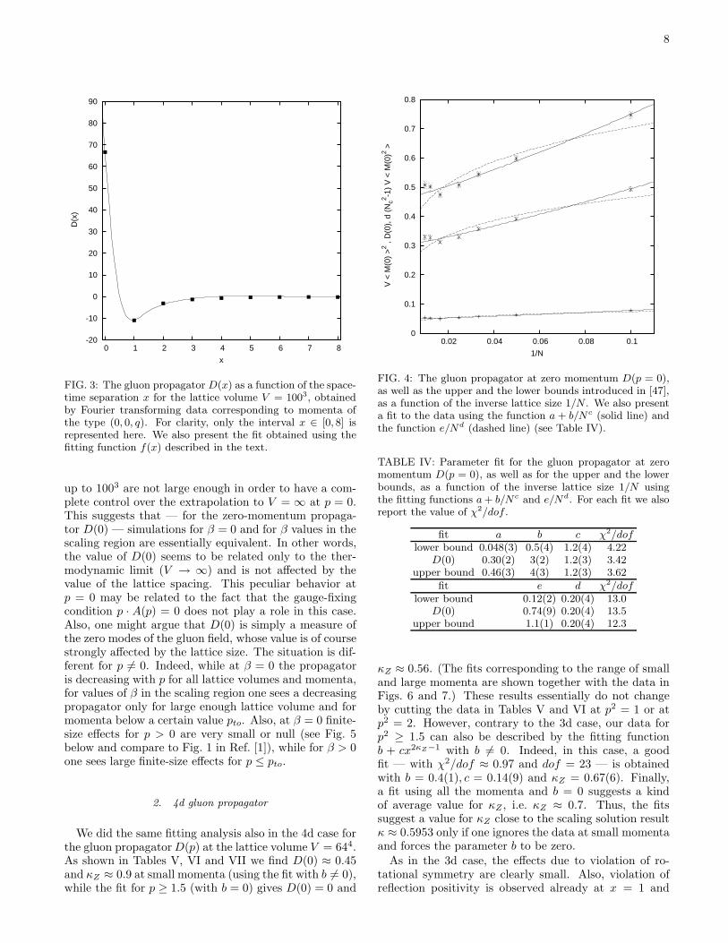
One can also check that the gluon propagator D(x) vi-olates reflection positivity. Actually, for all cases we findthat D(x = 1) is already negative. [Of course, D(x = 0)is always positive.] In Fig. 3 we show D(x) as a func-tion of the space-time separation x for the lattice volumeV = 1003 when considering momenta of the type (0, 0, q).Following Ref. [49], we fitted the data using a sum of twoStingl-like [89] propagators f(x) = f1(x) + f2(x) withfi(x) = ci cos (bi + λix) e−λix. We found a good de-scription of the data (see again Fig. 3) by fixing c1 =D(x = 0) = 66.6393, b1 = 0, b2 = π/2, λ2 = λ1/3 andwith c2 = 20(2) and λ1 = 2.5(2). Also, by comparingthese data to results obtained in the scaling region [49],one can use the value of x where D(x) starts to oscillatearound zero as an input for fixing the lattice spacing.From Fig. 3 this happens at x ≈ 3, giving a ≈ 1fm (seeFigure 5 in Ref. [49]). This is in quantitative agreementwith the values obtained in [73] (see Section I E above).

We also consider the volume dependence of D(p = 0)and the bounds introduced in [47]. As one can see fromFig. 4, these bounds are well satisfied. Compared to theresults obtained at finite (nonzero) β (see Fig. 1 in [47]),we find that the values of D(0) are closer to the upperbound than to the lower one. We have also checked thatwe can extrapolate the data for D(0) and for the upperand the lower bounds to a finite nonzero value as well asto zero (see Table IV). However, considering the valueof χ2/dof , our data seem to prefer an extrapolation toD(0) 6= 0 (see also Fig. 4).

Let us note that the above result is in agreement withwhat observed in Ref. [90], i.e. in the 3d case volumes

8

-20

-10

0

10

20

30

40

50

60

70

80

90

0 1 2 3 4 5 6 7 8

D(x

)

x

FIG. 3: The gluon propagator D(x) as a function of the space-time separation x for the lattice volume V = 1003, obtainedby Fourier transforming data corresponding to momenta ofthe type (0, 0, q). For clarity, only the interval x ∈ [0, 8] isrepresented here. We also present the fit obtained using thefitting function f(x) described in the text.

up to 1003 are not large enough in order to have a com-plete control over the extrapolation to V = ∞ at p = 0.This suggests that — for the zero-momentum propaga-tor D(0) — simulations for β = 0 and for β values in thescaling region are essentially equivalent. In other words,the value of D(0) seems to be related only to the ther-modynamic limit (V → ∞) and is not affected by thevalue of the lattice spacing. This peculiar behavior atp = 0 may be related to the fact that the gauge-fixingcondition p · A(p) = 0 does not play a role in this case.Also, one might argue that D(0) is simply a measure ofthe zero modes of the gluon field, whose value is of coursestrongly affected by the lattice size. The situation is dif-ferent for p 6= 0. Indeed, while at β = 0 the propagatoris decreasing with p for all lattice volumes and momenta,for values of β in the scaling region one sees a decreasingpropagator only for large enough lattice volume and formomenta below a certain value pto. Also, at β = 0 finite-size effects for p > 0 are very small or null (see Fig. 5below and compare to Fig. 1 in Ref. [1]), while for β > 0one sees large finite-size effects for p ≤ pto.

2. 4d gluon propagator

We did the same fitting analysis also in the 4d case forthe gluon propagator D(p) at the lattice volume V = 644.As shown in Tables V, VI and VII we find D(0) ≈ 0.45and κZ ≈ 0.9 at small momenta (using the fit with b 6= 0),while the fit for p ≥ 1.5 (with b = 0) gives D(0) = 0 and

0

0.1

0.2

0.3

0.4

0.5

0.6

0.7

0.8

0.02 0.04 0.06 0.08 0.1

V <

M(0

) >

2 , D

(0),

d (

Nc2 -1

) V

< M

(0)2 >

1/N

FIG. 4: The gluon propagator at zero momentum D(p = 0),as well as the upper and the lower bounds introduced in [47],as a function of the inverse lattice size 1/N . We also presenta fit to the data using the function a + b/Nc (solid line) andthe function e/Nd (dashed line) (see Table IV).

TABLE IV: Parameter fit for the gluon propagator at zeromomentum D(p = 0), as well as for the upper and the lowerbounds, as a function of the inverse lattice size 1/N usingthe fitting functions a + b/Nc and e/Nd. For each fit we alsoreport the value of χ2/dof .

fit a b c χ2/doflower bound 0.048(3) 0.5(4) 1.2(4) 4.22

D(0) 0.30(2) 3(2) 1.2(3) 3.42upper bound 0.46(3) 4(3) 1.2(3) 3.62

fit e d χ2/doflower bound 0.12(2) 0.20(4) 13.0

D(0) 0.74(9) 0.20(4) 13.5upper bound 1.1(1) 0.20(4) 12.3

κZ ≈ 0.56. (The fits corresponding to the range of smalland large momenta are shown together with the data inFigs. 6 and 7.) These results essentially do not changeby cutting the data in Tables V and VI at p2 = 1 or atp2 = 2. However, contrary to the 3d case, our data forp2 ≥ 1.5 can also be described by the fitting functionb + cx2κZ−1 with b 6= 0. Indeed, in this case, a goodfit — with χ2/dof ≈ 0.97 and dof = 23 — is obtainedwith b = 0.4(1), c = 0.14(9) and κZ = 0.67(6). Finally,a fit using all the momenta and b = 0 suggests a kindof average value for κZ , i.e. κZ ≈ 0.7. Thus, the fitssuggest a value for κZ close to the scaling solution resultκ ≈ 0.5953 only if one ignores the data at small momentaand forces the parameter b to be zero.

As in the 3d case, the effects due to violation of ro-tational symmetry are clearly small. Also, violation ofreflection positivity is observed already at x = 1 and

9

0.3

0.4

0.5

0.6

0.7

0.8

0.9

1

1.1

1.2

0 2 4 6 8 10 12

D(p

)

p2

FIG. 5: The gluon propagator D(p) as a function of the(unimproved) lattice momenta p2 for the lattice volumesV = 203 (symbol +), 403 (symbol ) and 803 (symbol ).Here all types of momenta are represented for the three latticevolumes considered.

TABLE V: Parameter fit for the gluon propagator D(p) as afunction of the (unimproved) lattice momentum p2 using thefitting function b + c(p2)2κZ−1 and data points in the rangep2 ∈ [0, 1.5] for the lattice volume 644. We do a separate fitfor each of the four types of momenta (0, 0, 0, q), (0, 0, q, q),(0, q, q, q) and (q, q, q, q), here indicated (respectively) as 1,2,3 and 4. For each fit we also report the number of degrees offreedom (dof) of the fit and the value of χ2/dof .

momenta b c κZ dof χ2/dof1 0.446(4) 0.095(5) 0.85(3) 11 1.332 0.460(5) 0.095(6) 0.83(4) 6 0.853 0.41(4) 0.14(4) 0.67(8) 4 1.284 0.45(2) 0.08(2) 0.9(2) 3 1.97

the gluon propagator in position space D(x) is well de-scribed by a sum of two Stingl-like propagators f(x) =f1(x)+f2(x) with fi(x) = ci cos (bi + λix) e−λix (see Fig.8). Note that the values of the masses λi are not very dif-ferent from the 3d case. Finally, as explained in SectionII C 1 above, one can fix the lattice spacing by comparingthese data to results obtained in the scaling region. Inparticular, considering our data at β = 2.2 for V = 1284,we find that D(x) ≈ 0 for x ∼> 2fm. Then, from Fig. 8,we find a ≈ 1fm as in the 3d case.

3. 3d ghost propagator

We now consider the data obtained for the ghostpropagator in the 3d case. [Note that in this case wedid not evaluate the propagator for the lattice volume

TABLE VI: Parameter fit for the gluon propagator D(p) asa function of the (unimproved) lattice momentum p2 usingthe fitting function c(p2)2κZ−1 and data points in the rangep2 ≥ 1.5 for the lattice volume 644. We do a separate fitfor each of the four types of momenta (0, 0, 0, q), (0, 0, q, q),(0, q, q, q) and (q, q, q, q), here indicated (respectively) as 1,2,3 and 4. For each fit we also report the number of degrees offreedom (dof) of the fit and the value of χ2/dof .

momenta c κZ dof χ2/dof1 0.533(3) 0.570(3) 17 0.762 0.558(4) 0.562(2) 21 0.863 0.561(6) 0.561(3) 23 0.994 0.531(6) 0.566(2) 24 0.97

TABLE VII: Parameter fit for the gluon propagator D(p) asa function of the (unimproved) lattice momentum p2 usingthe fitting function b + c(p2)2κZ−1 and all data points forthe lattice volume 644. We do a separate fit for each of thefour types of momenta (0, 0, 0, q), (0, 0, q, q), (0, q, q, q) and(q, q, q, q), here indicated (respectively) as 1,2, 3 and 4. Foreach fit we also report the number of degrees of freedom (dof)of the fit and the value of χ2/dof .

momenta b c κZ dof χ2/dof1 0.436(4) 0.103(5) 0.76(1) 30 1.602 0.430(9) 0.13(1) 0.70(1) 29 2.203 0.39(2) 0.17(2) 0.65(1) 29 1.384 0.41(1) 0.13(2) 0.68(1) 29 1.19

0.01

0.1

0 0.2 0.4 0.6 0.8 1

D(p

)

p2

FIG. 6: The gluon propagator D(p) as a function of the(unimproved) lattice momenta p2 for the lattice volume V =644 for momenta of the type (0, 0, 0, q) and p2 ≤ 1. We alsopresent the fits obtained at small momenta p2 ≤ 1.5 (solidline) and at large momenta p2 > 1.5 (dashed line). See Ta-bles V and VI.

10

0.5

1

1.5

2

2.5

3

1 1.5 2 2.5 3 3.5 4

D(p

)

p2

FIG. 7: The gluon propagator D(p) as a function of the(unimproved) lattice momenta p2 for the lattice volume V =644 for momenta of the type (0, 0, 0, q) and p2 ≥ 1. We alsopresent the fits obtained at small momenta p2 ≤ 1.5 (solidline) and at large momenta p2 > 1.5 (dashed line). See Ta-bles V and VI.

-5

0

5

10

15

20

25

30

35

40

45

0 1 2 3 4 5 6 7 8

D(x

)

x

FIG. 8: The gluon propagator D(x) as a function of the space-time separation x for the lattice volume V = 644, obtainedby Fourier transforming data corresponding to momenta ofthe type (0, 0, 0, q). For clarity, only the interval x ∈ [0, 8] isrepresented here. We also present the fit obtained using thefitting function f(x) described in the text with c1 = D(x =0) = 36.4604, b1 = 0, b2 = π/2, λ1 = 2.15(2), c2 = 1.7(1) andλ2 = 0.65(3).

1

10

100

1000

0.01 0.1 1

G(p

)

p2

FIG. 9: The ghost propagator G(p) as a function of the (unim-proved) lattice momenta p2 for the lattice volume V = 1003

for momenta of the type (0, 0, q). We also present the corre-sponding fit reported in Table VIII.

V = 303.] As said above, we tried a fit using the func-tion c(p2)−κG−1. Results are reported in Table VIII. Oneclearly sees that the infrared exponent κG decreases asthe lattice volume increases, in agreement with [38, 57].In this case the effects due to the violation of rotationalsymmetry are more evident. Indeed, the exponent κG issystematically smaller for momenta along the axes. Thisis probably due to the fact that along the axes one canconsider smaller momenta, for which the ghost propaga-tor is less enhanced.

By looking at Fig. 9 it is clear that this fit, with onlyone term, can be improved. In particular, consideringthe results reported in [1, 2, 3], one can try to see howthe exponent κG depends on the value of p2. To thisend we have ordered the data points by the value of p2

and divided them in sets of ten data points. Then, wedid a separate fit in each interval, again using the fittingfunction c(p2)−κG−1. Results for the lattice volume V =1003 are reported in Table IX. One clearly sees that theexponent κG increases with p2 (see also Fig. 10) and it isusually larger for the type of momenta (0, q, q). The sameis observed for the other lattice volumes. This result isactually well-known. Indeed, all lattice studies of theghost propagator [57, 91, 92] have found that G(p) isenhanced compared to the tree-level propagator 1/p2 atintermediate momenta. (We will comment again on thisin the Conclusions.)

11

TABLE VIII: Parameter fit for the ghost propagator G(p) asa function of the (unimproved) lattice momentum p2 using thefitting function c(p2)−κG−1 and all data. We do a separate fitfor each of the two types of momenta (0, 0, q), (0, q, q), hereindicated (respectively) as 1 and 2. In each case we indicatethe smallest nonzero momentum pmin. Finally, for each fitwe also report the number of degrees of freedom (dof) of thefit and the value of χ2/dof .

V momenta pmin c κG dof χ2/dof103 1 0.382 3.94(3) 0.260(8) 3 0.39103 2 0.764 3.9(1) 0.35(2) 3 1.75

203 1 0.098 3.77(5) 0.209(7) 8 4.15203 2 0.196 3.57(6) 0.28(1) 8 3.06403 1 0.0246 3.64(8) 0.171(7) 18 14.2403 2 0.0492 3.38(7) 0.220(8) 18 5.59603 1 0.0110 3.74(8) 0.144(5) 28 29.2603 2 0.0219 3.89(8) 0.192(8) 28 16.7

803 1 0.0062 3.84(9) 0.127(6) 38 18.4803 2 0.0123 3.50(7) 0.164(6) 38 7.021003 1 0.0039 4.1(1) 0.110(5) 48 19.41003 2 0.0079 3.46(8) 0.154(5) 48 9.91

0.1

1

10

100

1000

10000

0.01 0.1 1 10

G(p

)

p2

FIG. 10: The ghost propagator G(p) as a function of the(unimproved) lattice momenta p2 for the lattice volume V =1003 for momenta of the type (0, q, q). We also present thefits for the first and third sets of data points reported in TableIX.

4. 4d ghost propagator

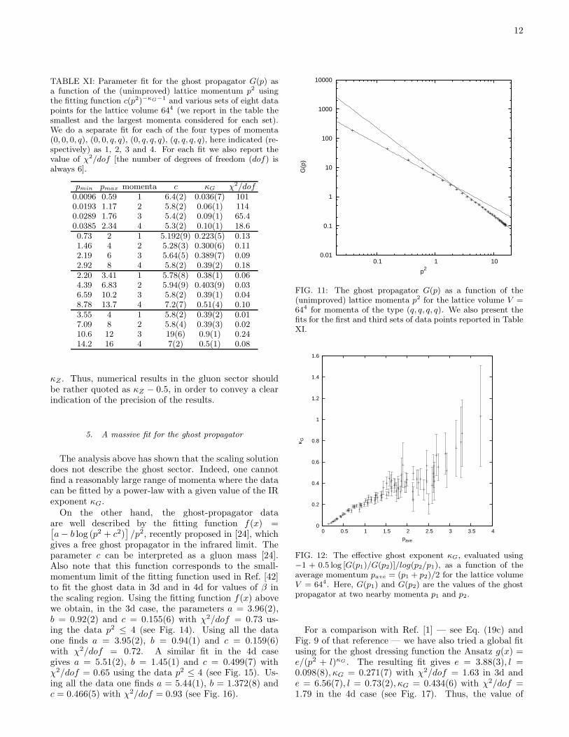
Finally, data for the ghost propagator G(p) in the 4dcase show again (see Table X) that the exponent κG de-pends on the type of momenta and systematically in-creases when one considers momenta closer to the di-agonal than to the axes. Also, the exponent κG in-creases with p2 (see Table XI and Fig. 11), going froma very small value — close to zero — at small p2 upto almost 1 for the largest momenta and for momenta

TABLE IX: Parameter fit for the ghost propagator G(p) asa function of the (unimproved) lattice momentum p2 usingthe fitting function c(p2)−κG−1 and various sets of ten datapoints for the lattice volume 1003 (we report in the table thesmallest and the largest momenta considered for each set).We do a separate fit for each of the two types of momenta(0, 0, q), (0, q, q), here indicated (respectively) as 1 and 2. Foreach fit we also report the value of χ2/dof [the number ofdegrees of freedom (dof) is always 8]. We do not report thefit for the last set because the corresponding data points havelarge statistical fluctuations.

pmin pmax momenta c κG χ2/dof0.0039 0.38 1 5.0(2) 0.070(6) 11.20.0079 0.76 2 4.4(1) 0.102(7) 4.400.46 1.38 1 4.00(2) 0.21(1) 0.170.92 2.76 2 3.98(5) 0.29(2) 0.191.50 2.62 1 3.7(1) 0.08(5) 0.193.01 5.24 2 4.2(1) 0.33(3) 0.042.74 3.62 1 6(1) 0.6(1) 0.315.47 7.24 2 3(1) 0.3(1) 0.28

TABLE X: Parameter fit for the ghost propagator G(p) asa function of the (unimproved) lattice momentum p2 usingthe fitting function c(p2)−κG−1 and all data for the latticevolume 644. We do a separate fit for each of the four typesof momenta (0, 0, 0, q), (0, 0, q, q), (0, q, q, q), (q, q, q, q), hereindicated (respectively) as 1, 2, 3 and 4. In each case weindicate the smallest nonzero momentum pmin. Finally, foreach fit we also report the value of χ2/dof [the number ofdegrees of freedom (dof) is always 30].

momenta pmin c κG χ2/dof1 0.0096 5.4(2) 0.075(7) 2502 0.0193 4.6(2) 0.128(9) 2383 0.0289 4.2(1) 0.16(1) 1274 0.0385 4.0(1) 0.19(1) 55.3

along the diagonal. This can be seen also in Fig. 12,where an effective exponent κG has been evaluated us-ing the relation −1 + 0.5 log [G(p1)/G(p2)]/log(p2/p1),where G(p1) and G(p2) are the values of the ghost prop-agator at two nearby momenta p1 and p2. The plot isdone as a function of the average momentum pave =(p1 + p2)/2. The errors have been evaluated using theso-called bootstrap method with 2000 samples. For clar-ity, we show only results with a relative error smallerthan 50% and with a positive value for κG (this crite-rion selects about 70% of the data). One clearly seesthat the effective exponent κG is monotonically increas-ing. The situation is very different in the gluon sector,where indeed a scaling solution can be used to fit thedata. As one can see in Fig. 13, the effective exponentκZ = 0.25 2 + log [D(p1)/D(p2)]/log(p1/p2) is essen-tially constant in this case. Moreover, at small momentaone finds κZ = 0.5, in agreement with the massive so-lution, and at large momenta the effective exponent isstill very close to this value. Note that a constant shiftof 0.5 is built into the definition of the gluon exponent

12

TABLE XI: Parameter fit for the ghost propagator G(p) asa function of the (unimproved) lattice momentum p2 usingthe fitting function c(p2)−κG−1 and various sets of eight datapoints for the lattice volume 644 (we report in the table thesmallest and the largest momenta considered for each set).We do a separate fit for each of the four types of momenta(0, 0, 0, q), (0, 0, q, q), (0, q, q, q), (q, q, q, q), here indicated (re-spectively) as 1, 2, 3 and 4. For each fit we also report thevalue of χ2/dof [the number of degrees of freedom (dof) isalways 6].

pmin pmax momenta c κG χ2/dof0.0096 0.59 1 6.4(2) 0.036(7) 1010.0193 1.17 2 5.8(2) 0.06(1) 1140.0289 1.76 3 5.4(2) 0.09(1) 65.40.0385 2.34 4 5.3(2) 0.10(1) 18.60.73 2 1 5.192(9) 0.223(5) 0.131.46 4 2 5.28(3) 0.300(6) 0.112.19 6 3 5.64(5) 0.389(7) 0.092.92 8 4 5.8(2) 0.39(2) 0.182.20 3.41 1 5.78(8) 0.38(1) 0.064.39 6.83 2 5.94(9) 0.403(9) 0.036.59 10.2 3 5.8(2) 0.39(1) 0.048.78 13.7 4 7.2(7) 0.51(4) 0.103.55 4 1 5.8(2) 0.39(2) 0.017.09 8 2 5.8(4) 0.39(3) 0.0210.6 12 3 19(6) 0.9(1) 0.2414.2 16 4 7(2) 0.5(1) 0.08

κZ . Thus, numerical results in the gluon sector shouldbe rather quoted as κZ − 0.5, in order to convey a clearindication of the precision of the results.

5. A massive fit for the ghost propagator

The analysis above has shown that the scaling solutiondoes not describe the ghost sector. Indeed, one cannotfind a reasonably large range of momenta where the datacan be fitted by a power-law with a given value of the IRexponent κG.

On the other hand, the ghost-propagator dataare well described by the fitting function f(x) =[

a − b log (p2 + c2)]

/p2, recently proposed in [24], whichgives a free ghost propagator in the infrared limit. Theparameter c can be interpreted as a gluon mass [24].Also note that this function corresponds to the small-momentum limit of the fitting function used in Ref. [42]to fit the ghost data in 3d and in 4d for values of β inthe scaling region. Using the fitting function f(x) abovewe obtain, in the 3d case, the parameters a = 3.96(2),b = 0.92(2) and c = 0.155(6) with χ2/dof = 0.73 us-ing the data p2 ≤ 4 (see Fig. 14). Using all the dataone finds a = 3.95(2), b = 0.94(1) and c = 0.159(6)with χ2/dof = 0.72. A similar fit in the 4d casegives a = 5.51(2), b = 1.45(1) and c = 0.499(7) withχ2/dof = 0.65 using the data p2 ≤ 4 (see Fig. 15). Us-ing all the data one finds a = 5.44(1), b = 1.372(8) andc = 0.466(5) with χ2/dof = 0.93 (see Fig. 16).

0.01

0.1

1

10

100

1000

10000

0.1 1 10

G(p

)

p2

FIG. 11: The ghost propagator G(p) as a function of the(unimproved) lattice momenta p2 for the lattice volume V =644 for momenta of the type (q, q, q, q). We also present thefits for the first and third sets of data points reported in TableXI.

0

0.2

0.4

0.6

0.8

1

1.2

1.4

1.6

0 0.5 1 1.5 2 2.5 3 3.5 4

κG

pave

FIG. 12: The effective ghost exponent κG, evaluated using−1 + 0.5 log [G(p1)/G(p2)]/log(p2/p1), as a function of theaverage momentum pave = (p1 + p2)/2 for the lattice volumeV = 644. Here, G(p1) and G(p2) are the values of the ghostpropagator at two nearby momenta p1 and p2.

For a comparison with Ref. [1] — see Eq. (19c) andFig. 9 of that reference — we have also tried a global fitusing for the ghost dressing function the Ansatz g(x) =e/(p2 + l)κG . The resulting fit gives e = 3.88(3), l =0.098(8), κG = 0.271(7) with χ2/dof = 1.63 in 3d ande = 6.56(7), l = 0.73(2), κG = 0.434(6) with χ2/dof =1.79 in the 4d case (see Fig. 17). Thus, the value of

13

FIG. 13: The effective gluon exponent κZ , evaluated using0.25 2 + log [D(p1)/D(p2)]/log(p1/p2), as a function of theaverage momentum pave = (p1 + p2)/2 for the lattice volumeV = 644. Here, D(p1) and D(p2) are the values of the gluonpropagator at two nearby momenta p1 and p2.

1

10

100

1000

0.01 0.1 1

G(p

)

p2

FIG. 14: The ghost propagator G(p) as a function of the(unimproved) lattice momenta p2 for the lattice volume V =1003 and momenta p2 ≤ 4. We also show a fit using thefitting function f(x) =

ˆ

a − b log (p2 + c2)˜

/p2, discussed inthe text.

χ2/dof is clearly worse when compared to the logarith-mic behavior considered above. In particular, from Fig.17 one can see that the power-law behavior cannot de-scribe well the “curvature” of the data, underestimatingthe data at small and at large momenta and overshootingthe numerical results at intermediate momenta. This isof course not a surprise since we have clearly shown inthe previous subsection that a single power-law does not

1

10

100

0.1 1

G(p

)

p2

FIG. 15: The ghost propagator G(p) as a function of the(unimproved) lattice momenta p2 for the lattice volume V =644 and momenta p2 ≤ 4. We also show a fit using the fit-ting function f(x) =

ˆ

a − b log (p2 + c2)˜

/p2, discussed in thetext.

describe the ghost data, unless one selects a very smallinterval of momenta. In the 4d case, this result doesnot improve if one forces the exponent κG to be equal to0.562, as done in Fig. 9 of [1]. Indeed, in this case wefind e = 8.37(6) and l = 1.23(2) with χ2/dof = 5.7 (seeFig. 18).

One should also observe that the function g(x) con-sidered above and in Ref. [1] is not a truly scaling solu-tion h(x) = s/(p2)κG . Indeed, while the latter is char-acterized by a constant value for the exponent κG =−∂ log[h(x)]/∂ log[p2] = −[p2/h(x)]∂h(x)/∂p2, for g(x)one has an effective exponent −[p2/g(x)]∂g(x)/∂p2 =κG p2/(p2 + l). This effective exponent is monotonicallyincreasing with p2, becoming constant and equal to κG

only for very large momenta. Thus, g(x) is trying todescribe the lattice data, characterized by an exponentκG increasing with the momentum, while “suggesting”a possible scaling behavior, i.e. a function with a con-stant exponent. In fact, as we have shown above, thedata are much better described by the massive solutionf(x), suggested by a recent analytic study [24]. On theother hand, a function such as g(x) is very poorly jus-tified from the theoretical point of view. In particular,such a fitting function for the ghost dressing functionimplies a fit e/[p2(p2 + l)κG ] for the ghost propagator.We do not see any theoretical reason that the mass scale√

l should affect only “part” of the power-law behaviorof the propagator. Here we have also tried a fit to theghost-propagator data using e/[(p2 + l)1+κG ]: the resultis very poor, with χ2/dof = 95.6 [and κG = 0.182(6)].

Finally, that a simple power-law is not capable of de-

14

0.1

0.2

0.4

0.8

0.1 1 10

1 /

p2 G(p

)

p2

FIG. 16: The inverse ghost dressing function 1/[p2G(p)] asa function of the (unimproved) lattice momenta p2 for thelattice volume V = 644. We also show a fit using the fittingfunction 1/

ˆ

a − b log (p2 + c2)˜

, discussed in the text.

scribing the lattice data should also be clear looking atFig. 5 of Ref. [1], where it is evident that the exponentκG depends on the momentum x considered, and fromFig. 9 of the same reference, where one sees that the fitsystematically underestimates the data at intermediatemomenta. Actually, at the end of Sec. III of Ref. [1] theauthors clearly say that a true scaling solution, i.e. theirEq. (19a), gives a very poor description of the ghost dataand that their preferred fitting function is g(x), whichonly reminds one of a possible scaling behavior. This isprobably the reason that induced the authors of [1] toconclude in favor of a scaling solution at large momentain the ghost sector. As already stressed above, we do notagree with this conclusion.

III. CONCLUSIONS

We have studied numerically the infrared behavior ofSU(2) Landau-gauge gluon and ghost propagators at lat-tice parameter β = 0, considering 3d lattices of volumesup to 1003 and 4d lattices of volume 644. By carrying outa careful fit analysis of the proposed behavior accordingto the scaling or to the massive solutions of DSE, we findthat our data strongly support the massive solution, i.e.a finite gluon propagator and an essentially free ghostpropagator in the infrared limit p → 0. Moreover, thegluon propagator D(x) as a function of the space-timeseparation x violates reflection positivity and it is well-described by a sum of two Stingl-like propagators. Theseresults are in qualitative agreement with data obtainedat finite β in the scaling region.

0.1

0.2

0.4

0.8

0.1 1 10

1 /

p2 G(p

)

p2

FIG. 17: The inverse ghost dressing function 1/[p2G(p)] asa function of the (unimproved) lattice momenta p2 for thelattice volume V = 644. We also show a fit using the fittingfunction g(x) = (p2 + l)κG/e, discussed in the text.

0.1

0.2

0.4

0.8

0.1 1 10

1 /

p2 G(p

)

p2

FIG. 18: The inverse ghost dressing function 1/[p2G(p)] asa function of the (unimproved) lattice momenta p2 for thelattice volume V = 644. We also show a fit using the fittingfunction g(x) = (p2 + l)0.562/e, discussed in the text.

We should stress that, in agreement with Refs. [1, 2, 3],a scaling solution appears in the gluon sector if one ne-glects the data at small momenta. As explain in Sec-tion I E above, we do not see any reason for excludingthose data from the analysis. In particular, discretiza-tion effects at small momenta are under control and the

15

large effects observed in Ref. [1] are probably only due tothe bad scaling properties of the modified Landau gauge.Moreover, the value of κ clearly depends on the way thefits are done. In particular, a value close to the preferredvalue of the scaling solution, i.e. 0.2(d − 1) in d dimen-sions, is obtained only with very specific and ad-hoc fits.In any case, we believe that the scaling solution is clearlyexcluded by the ghost sector and we definetively do notagree on this point with the analysis and the conclusionspresented in [1, 2, 3]. Indeed, in this case, the IR ex-ponent κ depends on the interval considered, increasingessentially monotonically as the momentum increases, i.e.it is impossible to find a decent “window” giving a con-stant value for κ. On the other hand, we have shown thatthe data for the ghost propagator are very well describedby a simple function, recently suggested by an analyticstudy presented in [24]. This function clearly supportsthe so-called massive solution.

As for the ongoing discussion about massive solutionversus conformal scaling, we remark that the lattice re-sults may be summarized as follows.

• In 2d Landau gauge one sees conformal scaling [42,46, 47],

• In 3d and 4d Landau gauge one finds the massivesolution [38, 39, 40, 42],

• In 4d Coulomb gauge, the transverse gluon propa-gator is well described by a Gribov formula, goingto zero at zero momentum [93, 94, 95]

• In the so-called λ gauges, which interpolate be-tween the Landau gauge (λ = 1) and the Coulombgauge (λ = 0), one clearly sees [96] that the behav-ior of the transverse gluon propagator gets modi-fied when λ goes from 1 to 0, becoming closer andcloser to the behavior obtained in Coulomb gaugeas λ becomes smaller and smaller.

The simulations cited above are essentially all done in thesame way, i.e. in most of the cases by ignoring effects dueto Gribov copies, by using a standard discretization forthe lattice action, for the gluon field and for the gauge-fixing condition and by using one of the standard gauge-fixing algorithms. Recently, to rescue the conformal so-lution in Landau gauge, several authors have explainedthe lattice Landau data by evoking supposedly (very)large effects due to Gribov copies, discretization effectsand bias related to the use of the usual gauge-fixing al-gorithms. Of course, one has to verify that all possiblesources of systematic effects are indeed under control ina numerical simulation. On the other hand, it seemsunlikely to us that these effects would show up in somecases of the simulations described above and not in oth-ers. For example, why would the 2d Landau-gauge case

be conformal and not the 3d and 4d cases if the samecode is used in these three cases? Why should Gribov-copy effects be so important in 3d and 4d Landau gaugeand not in 2d Landau gauge and, even more strikingly,in 4d Coulomb gauge, where one would expect strongereffects since the transversality condition is imposed sep-arately on each time slice? In our view, present latticedata are simply telling us that the infrared behavior ofgluon and ghost propagators in Landau, Coulomb and λgauge depends on the gauge-fixing condition and on thedimensionality of the system (as, for example, the criticalbehavior of statistical mechanical systems). We believethat the present challenge is to understand why this isthe case and that the bounds introduced by us in Ref.[47] and their interpretation in terms of magnetizationand susceptibility of the gluon field could be a key ingre-dient in a simple explanation of present lattice results inLandau gauge.

Finally a remark about color confinement. As said inthe Conclusion of Ref. [42], we point out that the be-havior of gluon and ghost propagators at very small mo-menta is probably not so important for the explanationof confinement. Indeed, why should the behavior of aGreen function at a few MeV , i.e. for a space separa-tion of about 50fm, be relevant for hadron physics, sincethe typical hadronic scale is of order of 1fm? Let us re-call that in a recent paper [97] it has been shown thatthe appearance of a linearly-rising potential is related (inLandau and in Coulomb gauge) to the momentum-spacegluon configuration A(p) for p ∼< 1 GeV . In this regionone can indeed observe strong non-perturbative effects inthe gluon and in the ghost propagators in Landau gauge:the gluon propagator violates reflection positivity andthe ghost propagator is enhanced when compared to thetree-level behavior. Thus, some important predictions ofthe Gribov-Zwanziger scenario are still verified and, atthe same time, one can try to relate the massive solu-tion to the requirement of color confinement as in Refs.[30, 31, 32].

IV. ACKNOWLEDGEMENTS

We thank the organizers of the workshop on Non per-turbative Aspects of Field Theories (Morelia ’09), wherethis work was presented, for providing a very stimulatingatmosphere for discussions, in such a beautiful setting.

We acknowledge partial support from the BrazilianFunding Agencies FAPESP and CNPq. The work ofT.M. is supported also by a fellowship from the Alexan-der von Humboldt Foundation. Most of the simulationsreported here have been done on the IBM supercomputerat Sao Paulo University (FAPESP grant # 04/08928-3).

[1] A. Sternbeck and L. von Smekal, arXiv:0811.4300 [hep-lat].

[2] A. Sternbeck and L. von Smekal, PoS LATTICE2008,

16

267 (2008).[3] A. Sternbeck and L. von Smekal, arXiv:0812.3268 [hep-

lat].[4] V.N. Gribov, Nucl. Phys. B 139, 1 (1978).[5] D. Zwanziger, Nucl. Phys. B 412, 657 (1994).[6] D. Zwanziger, arXiv:0904.2380 [hep-th].[7] For a short review of the Gribov-Zwanziger approach see

A. Cucchieri and T. Mendes, arXiv:0809.2777 [hep-lat].[8] T. Kugo and I. Ojima, Prog. Theor. Phys. Suppl. 66, 1

(1979) [Erratum-ibid. 71, 1121 (1984)].[9] T. Kugo, arXiv:hep-th/9511033.

[10] R. Alkofer and L. von Smekal, Phys. Rept. 353, 281(2001).

[11] D. Zwanziger, Phys. Rev. D 67, 105001 (2003).[12] D. Zwanziger, Phys. Lett. B 257, 168 (1991).[13] G. Dell’Antonio and D. Zwanziger, Nucl. Phys. B 326,

333 (1989).[14] D. Dudal, S.P. Sorella, N. Vandersickel and H. Ver-

schelde, arXiv:0904.0641 [hep-th].[15] See for example C.D. Roberts and A.G. Williams, Prog.

Part. Nucl. Phys. 33, 477 (1994).[16] R. Alkofer, M.Q. Huber and K. Schwenzer, arXiv:0801.

2762 [hep-th].[17] C.S. Fischer and J.M. Pawlowski, Phys. Rev. D 75,

025012 (2007).[18] L. von Smekal, A. Hauck and R. Alkofer, Annals Phys.

267, 1 (1998) [Erratum-ibid. 269, 182 (1998)].[19] D. Zwanziger, Phys. Rev. D 65, 094039 (2002).[20] J.M. Pawlowski et al., Phys. Rev. Lett. 93, 152002

(2004).[21] A.C. Aguilar and A.A. Natale, JHEP 0408, 057 (2004).[22] Ph. Boucaud et al., JHEP 0606, 001 (2006).[23] C.S. Fischer, J. Phys. G 32, R253 (2006).[24] A.C. Aguilar, D. Binosi and J. Papavassiliou, Phys. Rev.

D 78, 025010 (2008).[25] M.Q. Huber et al., Phys. Lett. B 659, 434 (2008).[26] Ph. Boucaud et al. JHEP 0806, 012 (2008).[27] Ph. Boucaud et al., JHEP 0806, 099 (2008).[28] C.S. Fischer, A. Maas and J.M. Pawlowski, arXiv:0810.

1987 [hep-ph].[29] R. Alkofer and J. Greensite, J. Phys. G 34, S3 (2007).[30] M. Chaichian and K. Nishijima, Eur. Phys. J. C 47, 737

(2006).[31] J.M. Cornwall, Nucl. Phys. B 157, 392 (1979).[32] J. Braun, H. Gies and J.M. Pawlowski, PoS CONFINE-

MENT8, 044 (2008).[33] D. Dudal et al., Phys. Rev. D 77, 071501 (2008).[34] D. Dudal et al., Phys. Rev. D 78, 065047 (2008).[35] D. Dudal et al., Phys. Rev. D 78, 125012 (2008).[36] D. Dudal et al., arXiv:0808.3379 [hep-th].[37] M. Frasca, Phys. Lett. B 670, 73 (2008).[38] A. Cucchieri and T. Mendes, PoS (LATTICE 2007) 297.[39] I.L. Bogolubsky et al., PoS LAT2007, 290 (2007).[40] A. Sternbeck et al., PoS LAT2007, 340 (2007).[41] O. Oliveira and P.J. Silva, arXiv:0705.0964 [hep-lat].[42] A. Cucchieri and T. Mendes, Phys. Rev. D 78, 094503

(2008).[43] V.G. Bornyakov, V.K. Mitrjushkin and M. Muller-Preus-

sker, arXiv:0812.2761 [hep-lat].[44] I.L. Bogolubsky, E.M. Ilgenfritz, M. Muller-Preussker

and A. Sternbeck, Phys. Lett. B 676, 69 (2009).[45] M. Gong et al., arXiv:0811.4635 [hep-lat].[46] A. Maas, Phys. Rev. D 75, 116004 (2007).[47] A. Cucchieri and T. Mendes, Phys. Rev. Lett. 100,

241601 (2008).[48] K. Langfeld, H. Reinhardt and J. Gattnar, Nucl. Phys.

B 621, 131 (2002).[49] A. Cucchieri, T. Mendes and A.R. Taurines, Phys. Rev.

D 71, 051902 (2005).[50] O. Oliveira and P.J. Silva, Braz. J. Phys. 37, 201 (2007).[51] P.O. Bowman et al., Phys. Rev. D 76, 094505 (2007).[52] A. Cucchieri, Nucl. Phys. B 521, 365 (1998).[53] A. Sternbeck, E.M. Ilgenfritz and M. Muller-Preussker,

Phys. Rev. D 73, 014502 (2006).[54] A. Cucchieri, A. Maas and T. Mendes, Phys. Rev. D 74,

014503 (2006).[55] A. Cucchieri and T. Mendes, arXiv:0812.3261 [hep-lat].[56] A. Cucchieri, AIP Conf. Proc. 892, 22 (2007).[57] A. Cucchieri, Nucl. Phys. B 508, 353 (1997).[58] P.J. Silva and O. Oliveira, Nucl. Phys. B 690, 177 (2004).[59] P.J. Silva and O. Oliveira, PoS LAT2007, 333 (2007).[60] A. Maas, arXiv:0808.3047 [hep-lat]. Phys. Rev. D 79,

014505 (2009).[61] D.B. Leinweber et al., Phys. Rev. D 60, 094507 (1999)

[Erratum-ibid. D 61, 079901 (2000)].[62] J.P. Ma, Mod. Phys. Lett. A 15, 229 (2000).[63] F. de Soto and C. Roiesnel, JHEP 0709, 007 (2007).[64] E. Shintani et al., arXiv:0807.0556 [hep-lat].[65] F. Di Renzo, Nucl. Phys. Proc. Suppl. 53 (1997) 819.[66] L. Giusti et al., Phys. Lett. B 432, 196 (1998).[67] S. Furui and H. Nakajima, Nucl. Phys. Proc. Suppl. 73,

865 (1999).[68] F.D.R. Bonnet et al., Austral. J. Phys. 52, 939 (1999).[69] A. Cucchieri and F. Karsch, Nucl. Phys. Proc. Suppl. 83,

357 (2000).[70] L. von Smekal et al., PoS LAT2007, 382 (2007).[71] J.C.R. Bloch et al., Nucl. Phys. B 687, 76 (2004).[72] A. Cucchieri, Phys. Lett. B 422, 233 (1998).[73] P. de Forcrand and M. Fromm, arXiv:0907.1915 [hep-lat].[74] P. de Forcrand and S. Kim, Phys. Lett. B 645, 339

(2007).[75] A. Cucchieri and T. Mendes, in preparation.[76] See for example the introduction to strong-coupling ex-

pansion in Introduction to Quantum Fields on a Lattice,Jan Smit (Cambridge University Press, 2002, CambridgeUK).

[77] A. Cucchieri, poster presented at the workshop InfraredQCD in Rio, held in Rio de Janeiro in June 2006(http://www.dft.if.uerj.br/irqcd06/).

[78] A. Cucchieri et al., Phys. Rev. D 76, 114507 (2007).[79] A. Cucchieri et al., PoS LAT2007, 322 (2007).[80] A. Maas and S. Olejnik, JHEP 0802, 070 (2008).[81] A. Cucchieri, T. Mendes, O. Oliveira and P.J. Silva, Int.

J. Mod. Phys. E 16, 2931 (2007).[82] A. Cucchieri and T. Mendes, Nucl. Phys. B 471, 263

(1996).[83] Ph. Boucaud et al., Phys. Rev. D 72, 114503 (2005).[84] M. Creutz, Phys. Rev. D 21, 2308 (1980).[85] See the Introduction of A. Cucchieri and T. Mendes,

Comput. Phys. Commun. 154, 1 (2003).[86] A. Cucchieri and T. Mendes, Nucl. Phys. Proc. Suppl.

53, 811 (1997).[87] T. Mendes et al., arXiv:0809.3741 [hep-lat].[88] See for example D. Becirevic et al., Phys. Rev. D 60,

094509 (1999).[89] M. Stingl, Phys. Rev. D 34, 3863 (1986) [Erratum-ibid.

D 36, 651 (1987)].[90] A. Cucchieri, T. Mendes and A.R. Taurines, Phys. Rev.

17

D 67, 091502 (2003).[91] S. Furui and H. Nakajima, Phys. Rev. D 69, 074505

(2004).[92] J. Gattnar, K. Langfeld and H. Reinhardt, Phys. Rev.

Lett. 93, 061601 (2004).[93] A. Cucchieri and D. Zwanziger, Phys. Rev. D 65, 014001

(2002).[94] A. Cucchieri and D. Zwanziger, Phys. Lett. B 524, 123

(2002).

[95] G. Burgio, M. Quandt and H. Reinhardt, Phys. Rev.Lett. 102, 032002 (2009).

[96] A. Cucchieri, A. Maas and T. Mendes, Mod. Phys. Lett.A 22, 2429 (2007).

[97] A. Yamamoto and H. Suganuma, Phys. Rev. Lett. 101,241601 (2008).

[98] Data have been extracted from the plots using the g3dataprogram.