arX

iv:h

ep-t

h/96

0116

2v1

30

Jan

1996

ROM2F-95-30

Explicit Construction of

Yang-Mills Instantons on ALE Spaces

Massimo Bianchi, Francesco Fucito, Giancarlo Rossi

Dipartimento di Fisica, Universita di Roma II “Tor Vergata”

I.N.F.N. - Sezione di Roma II,

Via Della Ricerca Scientifica 00133 Roma ITALY

Maurizio Martellini 1

The Niels Bohr Institute, University of Copenhagen

DK-2100 Copenhagen φ, Denmark

I.N.F.N. - Sezione di Milano

Landau Network at “Centro Volta”, Como ITALY

ABSTRACT

We describe the explicit construction of Yang-Mills instantons on Asymptot-

ically Locally Euclidean (ALE) spaces, following the work of Kronheimer and

Nakajima. For multicenter ALE metrics, we determine the abelian instanton

connections which are needed for the construction in the non-abelian case.

We compute the partition function of Maxwell theories on ALE manifolds

and comment on the issue of electromagnetic duality. We discuss the topo-

logical characterization of the instanton bundles as well as the identification

of their moduli spaces. We generalize the ’t Hooft ansatz to SU(2) instan-

tons on ALE spaces and on other hyper-Kahler manifolds. Specializing to

the Eguchi-Hanson gravitational background, we explicitly solve the ADHM

equations for SU(2) gauge bundles with second Chern class 1/2, 1 and 3/2.

1On leave of absence from Dipartimento di Fisica, Universita di Milano, 20133 Milano,

Italy

1 Introduction

Asymptotically Locally Euclidean (ALE) gravitational instantons have played

a fundamental role in Euclidean quantum supergravity (for a review see [1]).

They induce non-perturbative effects which turn out to be very relevant for

understanding the vacuum structure of the theory and are possibly responsi-

ble for the emergence of dynamical breaking mechanisms for supersymmetry

(SUSY). From a mathematical point of view they are interesting non-compact

hyper-Kahler manifolds which admit a complete classification, induced by the

A-D-E classification of simply-connected Lie algebras.

In a recent work [2] we have shown that ALE metrics can be incorporated

in a fully supersymmetric solution of the four-dimensional heterotic string

equations of motion with constant dilaton and zero torsion (for a review of

SUSY solutions of low energy supergravities see [3]). Thanks to the so-called

standard embedding condition, this solution can be shown to be an exact

one (corresponding to an exact N = (4, 4) superconformal field theory on

the world-sheet, see also [4, 5]), to all orders in (the σ-model coupling) α′.

To study whether these backgrounds might eventually lead to the the

formation of chiral condensates, instanton dominated correlation functions

must be computed. For globally supersymmetric Yang-Mills (YM) theories

with N = 1, 2, 4 we have performed this computation around the minimal

instanton on the Eguchi-Hanson (EH) manifold [6], the simplest of all possible

ALE spaces. The denomination minimal instanton comes from the value

of its second Chern class, κ = 1/2, which is the minimal one allowed for

SU(2) bundles on the EH manifold. The minimal instanton plays on the EH

background the same role as the t’Hooft-Polyakov instanton on flat space.

It was also found, by quite different methods, in [7]. The results of the

instantonic computations presented in [6] are analogous to those obtained

in flat spacetime [8]: the chiral condensates are constant and turn out to be

2

proportional to the appropriate power of the renormalization group invariant

scale of the theory, as dictated by naive dimensional counting.

The extension of instanton computations to fullfledged solutions of the

heterotic string equations of motion [2], is not straightforward. It requires,

as we said, the embedding of the spin connection into the gauge group,

and it is based on the fact that the self-dual spin connection of an ALE

gravitational background lies in the SU(2)L factor of the SO(4) Lorentz

group. The relevant SU(2) gauge bundle is then the holomorphic tangent

bundle to the ALE manifold. In the case of the EH background the dimension

of the moduli space of the gauge connections on the tangent bundle was

computed, via index formulae, to be 12 and its second Chern class turned out

to be κ = 3/2 [2]. Computation of instanton effects requires the knowledge

of the form of the gauge connection. This is the task we tackle in the present

paper where we build all SU(2) gauge bundles up to κ = 3/2 and clarify the

quite intricate mathematics needed to do it. To carry out this program we will

use recent results of Kronheimer and Nakajima who, in a series of beautiful

papers [9, 10, 11], completely solved the problem of constructing self-dual

YM connections on ALE manifolds along the lines of the analogous Atiyah-

Drinfeld-Hitchin-Manin (ADHM) construction [12, 13] of gauge instantons

on flat space.

The plan of the paper is as follows. In section 2 we review the construc-

tion of ALE gravitational instantons. Using twistor techniques, Hitchin [14]

has shown that ALE manifolds are smooth resolutions of algebraic varieties

in C3. Simple singularities admit an A-D-E classification according to which,

the class of multicenter metrics of Gibbons-Hawking (GH) [15] (to which the

EH instanton [16] belongs) may be identified with the resolution of singulari-

ties of A-type. A general construction of all ALE manifolds was then worked

out by Kronheimer [17]. These manifolds emerge as minimal resolutions

3

of C2/Γ, where the discrete subgroups Γ of SU(2) are in one-to-one corre-

spondence with the extended Dynkin diagrams of simply-laced (i.e. A-D-E)

simple Lie algebras. ALE spaces are explicitly obtained as hyper-Kahler quo-

tients of flat Euclidean spaces. This allows, in principle, the determination

of the hyper-Kahler metric on them. In practice only for ALE spaces of A-

type, corresponding to Γ = ZN , the metric is known and it turns out to be

diffeomorphic to the GH multicenter metric.

The hyper-Kahler quotient construction allows to identify a principal bun-

dle over the ALE space whose natural connection has anti-self-dual curvature.

To this principal bundle, a tautological vector bundle, T , can be associated

by a change of fiber. This bundle admits a decomposition under the action

of Γ into r (=rank(Γ)) elementary bundles, Ti, whose first Chern classes form

a basis for the second cohomology group of the ALE space. For multicen-

ter ALE metrics the bundles Ti admit abelian connections that we explicitly

construct in section 3. They will be needed in the following to compute

the gauge connections in non-abelian cases. As a byproduct we obtain a

formula for the partition function of abelian gauge theories on ALE spaces,

in terms of the level one characters of the affine Lie algebra of the type A-

D-E, associated to the ALE space under consideration, and we show that

electromagnetic duality, at least in its simplest form, does not hold on ALE

spaces.

In Section 4 we recall the essential steps of the ADHM construction of

gauge instantons on R4 and argue that this construction can be viewed as

an hyper-Kahler quotient. This observation establishes a bridge with the

Kronheimer-Nakajima (KN) construction of YM instantons on ALE spaces

which is discussed immediately afterwards. We then elaborate on some

known solutions, generalizing the ansatze of ’t Hooft [18] and Jackiw, Nohl

and Rebbi [19] to four-dimensional hyper-Kahler manifolds (including ALE

4

gravitational instantons) and discuss some Γ-invariant instantons on R4.

In section 5 by studying the topological properties of the gauge instanton

bundles, we are able to identify some already known solutions. We emphasize

the role of the discrete group Γ and compute the topological invariants of

these bundles, the dimensions of their moduli spaces and, in the SU(2) case,

the indices of the relevant Dirac operators.

In section 6 we explicitly solve the ADHM equations for SU(2) gauge

bundles with second Chern class up to κ = 3/2 on the EH background.

Following the KN-ADHM construction the problem is reduced to a bunch of

conceptually simple but somewhat tedious algebraic manipulations.

In section 7 we discuss some properties of the moduli spaces of YM in-

stanton connections on ALE spaces and exhibit the hyper-Kahler metric for

the minimal instanton on the EH background and in section 8 we draw our

conclusions.

In the appendix we show how to recover the explicit form of the EH

metric, following the hyper-Kahler quotient construction.

2 Kronheimer Construction of ALE Instan-

tons

2.1 Hyper-Kahler Quotients

A Riemannian manifold X is said to be hyper-Kahler if it is equipped with

three covariantly constant complex structures I, J,K, i.e. automorphisms of

the tangent bundle satisfying the quaternionic algebra I2 = J2 = K2 = −11

and IJ = −K, JK = −I,KI = −J . In this circumstance the metric g on X

is said to be of Kahler type (or simply, Kahler) with respect to I, J,K and

5

one can define three closed Kahler 2-forms

ωI(V,W ) = g(V, IW )

ωJ(V,W ) = g(V, JW )

ωK(V,W ) = g(V,KW ) (2.1)

with V,W vector fields on X. We will often denote the hyper-Kahler forms

in (2.1) as ωi, with i = I, J,K. In four dimensions a simply-connected

Riemannian manifold is hyper-Kahler when its Riemann curvature tensor is

either self-dual or anti-self-dual2. A four-dimensional hyper-Kahler manifold

is thus a gravitational instanton.

In this section we want to briefly recall the Kronheimer [17] construction

of a particular family of hyper-Kahler manifolds, the so called ALE gravita-

tional instantons.

We begin by discussing a method to produce a hyper-Kahler manifold

X of real dimensions d = 4(n − k) starting from a 4n-dimensional hyper-

Kahler manifold Ξ [20]. The manifold X is obtained as the quotient of a

real subspace of Ξ by some subgroup of the isometry group of Ξ. In this

procedure a central role is played by the moment map. By assumption Ξ

admits vector fields V , known as Killing vectors, which generate isometries,

i.e. for which LV g = 0, with LV the Lie derivative along V . Killing vector

fields are said to be triholomorphic if furthermore LV ωi = iV dωi + d(iV ωi) =

0, where iV denotes contraction with V . To each vector of this kind there

correspond three Killing potentials, µVi , which can be obtained by integrating

2In the mathematical literature, instantons on complex manifolds denote YM con-

nections whose field-strength is anti-self-dual in the natural orientation of the manifold,

inherited from its complex structure. In these conventions, (ALE) gravitational instan-

tons, which are complex hyper-Kahler manifolds, turn out to have anti-self-dual curvature.

We will follow, instead, the physicists’ conventions of inverting the natural orientation and

call instantons, either YM or gravitational, connections with self-dual curvature.

6

the equations

dµVi = iV ωi (2.2)

following from dωi = 0 and LV ωi = 0. In the absence of abelian factors,

the integration constants may be fixed requiring WµVi = µ

[V,W ]i . The Killing

potentials µVi = µi define a hyper-Kahler moment map

µi : ξ ∈ Ξ 7→ µai (ξ) ∈ R

3 × G∗ i = 1, 2, 3 a = 1, . . . , dim(G) (2.3)

where G∗ is the dual to the Lie algebra, G, of the isometry group G gener-

ated by the triholomorphic vectors, V . The moment maps in (2.3) can be

suggestively reorganized in the combinations µR = µ3 and µC = µ1 + iµ2.

Let us make an example to clarify the meaning of these concepts. In

Hamiltonian mechanics, there is a natural two form:

ω = dpi ∧ dqi (2.4)

where the qi’s and the pi’s are the generalized coordinates and momenta. If

we take the isometries to be translations, V = ai ∂∂qi

, then iV ω = aidpi = dµ

and µ is the usual linear momentum, whence the name. If the V ’s were the

generators of the rotation group, SO(3), then the moment map would be

given by ~µ = ~q ∧ ~p, i.e. by the angular momentum. It should be clear now

that the moment map construction is a way of generalizing the procedure of

identifying conserved quantities in classical mechanics.

Any hyper-Kahler manifold Ξ admitting a compact group G of k freely

acting triholomorphic isometries, contains a hyper-Kahler submanifold X of

real dimension

dim(X) = dim(Ξ) − 4dim(G) = 4n− 4k (2.5)

which is the hyper-Kahler quotient of Ξ with respect to G. The construction

of X proceeds in two steps. First a submanifold Pζ of dimension dim(Pζ) =

7

dim(Ξ) − 3dim(G) = 4n − 3k, is identified as the level set of 3 × k hyper-

Kahler moment maps, i.e.

Pζ = ξ ∈ Ξ | µai (ξ) = ζa

i , i = 1, 2, 3 a = 1, . . . , k (2.6)

When the ζ ’s belong to R3 × Z∗, with Z∗ the dual to the center of G, the

hypersurface Pζ is left invariant by the action of G. In fact Pζ turns out to be

a G-principal bundle. If one divides out the group G from Pζ , one obtains a

new hyper-Kahler manifold, Xζ = Pζ/G. Notice that the algebro-geometric

quotient Nζ/GC, with

Nζ = ξ ∈ Ξ | µaC(ξ) = ζa

C, a = 1, . . . , k (2.7)

and GC the complexification of G, is diffeomorphic to Xζ . As a by-product

of this construction one finds that the curvature of the natural connection

on the principal bundle Pζ over Xζ is self-dual [20, 11].

2.2 A-D-E Classification of ALE Gravitational Instan-

tons

Kronheimer constructed all ALE gravitational instantons as particular hyper-

Kahler quotients [17]. Given a discrete Kleinian subgroup of SU(2), i.e. Γ =

ZN , D∗N , O

∗, T ∗, I∗, consider the flat hyper-Kahler space

Ξ = (Q⊗ End(R))Γ (2.8)

where Q(∼ C2) is the vector space of the fundamental two-dimensional rep-

resentation, ρQ, of Γ and End(R) is the set of endomorphisms of the vec-

tor space, R, of the regular representation, ρR, of Γ. Ξ is the space of Γ-

invariant pairs of endomorphisms of R. Since for the regular representation

8

dim(R) = dim(Γ) = |Γ|, the elements of Ξ can be represented as doublets of

the form

ξ =

(α

β

)(2.9)

where α, β are |Γ|×|Γ| complex matrices satisfying the Γ-invariance property3

(ρR(γ)αρ

R(γ−1)

ρR(γ)βρ

R(γ−1)

)= ρ

Q(γ)

(α

β

)γ ∈ Γ (2.10)

The points ξ of the manifold Ξ can also be represented by quaternions of

matrices

ξ =

(α −β†

β α†

)(2.11)

so that Ξ can also be viewed as the space Ξ = (T ∗ ⊗R Endskew(R))Γ, with

T the quaternionic space and T ∗ its dual.

The role of the discrete subgroup Γ ⊂ SU(2) in (2.10), is clarified by the

Mac Kay correspondence [21] between Kleinian subgroups Γ ⊂ SU(2) and

A-D-E extended Dynkin diagrams, ∆Γ.

We recall that, given a representation ρW

of Γ, in order to find its de-

composition, ρW

= ⊕r−1i=0wiρi, in irreducible representations of Γ (ρ

Ri≡ ρi,

where ρo is the trivial representation), we must look at the extended Dynkin

diagram, ∆Γ, of the A-D-E Lie algebra associated to Γ. In the above decom-

position r is the rank of Γ, i.e. the number of conjugacy classes of Γ. The

extended Dynkin diagram is constructed, starting from the standard Dynkin

diagram, ∆Γ, according to the following steps

i) an extra dot, corresponding to minus the highest root of the algebra

(called the extended root, α0), is added to ∆Γ;

3With an abuse of notations we will sometimes call the vector space, R, that carries the

representation ρR, the “representation R” and use the symbol R also for the representation

matrix, ρR.

9

ii) a number, ni, equal to half the sum of the numbers attributed to the

neighbouring roots is associated to each dot of ∆Γ, starting from the

assignment n0 = 1 made to the extended root.

In this way one finds α0 = −∑r−1i=1 niαi and the numbers ni turn out to

coincide with the dimensions of the irreducible representations ρi of Γ. In

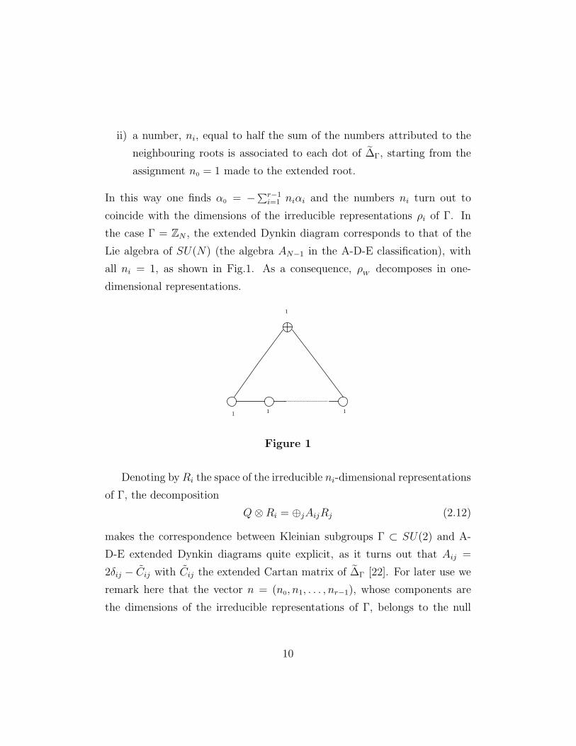
the case Γ = ZN , the extended Dynkin diagram corresponds to that of the

Lie algebra of SU(N) (the algebra AN−1 in the A-D-E classification), with

all ni = 1, as shown in Fig.1. As a consequence, ρW

decomposes in one-

dimensional representations.

.............................

1 1 1

1

Figure 1

Denoting by Ri the space of the irreducible ni-dimensional representations

of Γ, the decomposition

Q⊗Ri = ⊕jAijRj (2.12)

makes the correspondence between Kleinian subgroups Γ ⊂ SU(2) and A-

D-E extended Dynkin diagrams quite explicit, as it turns out that Aij =

2δij − Cij with Cij the extended Cartan matrix of ∆Γ [22]. For later use we

remark here that the vector n = (n0, n1, . . . , nr−1), whose components are

the dimensions of the irreducible representations of Γ, belongs to the null

10

space of the extended Cartan matrix, i.e.∑r−1

j=0 Cijnj = 0 4.

The vector space carrying the regular representation admits the decom-

position

R = ⊕iRi ⊗ Ri (2.13)

In the following we will be interested in the action of Γ by left multiplication

only. Since left multiplication leaves Ri untouched, one can simply write

R = ⊕iRi⊗Cni. In this respect Γ can be taken to be a subgroup of the same

SU(2)L factor of the Lorentz group in which the self-dual spin connection of

the resulting ALE instanton will lie.

Imposing Γ-invariance in the form of (2.10), one finds the decomposition

Ξ = ⊕ijAijHom(Cni ,Cnj ) (2.14)

which shows that the (real) dimension of Ξ is

dim(Ξ) = 2r−1∑

i,j=0

Aijninj = 4r−1∑

i=0

(ni)2 = 4|Γ| (2.15)

To prove (2.14) we write successively

Ξ = (Q⊗ End(R))Γ = (Q⊗ Hom(⊕iRi ⊗ Cni,⊕jRj ⊗ C

nj ))Γ

= (Q⊗ (⊕ijHom(Ri, Rj)))Γ ⊗ Hom(Cni ,Cnj )

= (⊕ijkAikHom(Rk, Rj))Γ ⊗ Hom(Cni,Cnj ) (2.16)

having used the decomposition (2.12). Since Hom(Ri, Rj)Γ = δij thanks to

Schur’s lemma, equation (2.14) immediately follows.

Using the representation (2.11), the three hyper-Kahler forms on Ξ can

be written

ωi = Tr(dξ† ∧ dξσPi ) i = 1, 2, 3 (2.17)

4From now on, unless differently stated, all the sums and products over indices labelling

the irreducible representations of Γ are understood to be extended from 0 to r − 1.

11

where the σPi ’s are the standard Pauli matrices. They can be combined into

a real (1, 1)-form and a complex (2, 0)-form as follows

ωR = Tr(dα ∧ dα†) + Tr(dβ ∧ dβ†)

ωC = Tr(dα ∧ dβ) (2.18)

The action of a generic elements g ∈ U(|Γ|) on ξ ∈ Ξ is induced by the

transformations

α→ gαg†, β → gβg† (2.19)

and leaves invariant the hyper-Kahler forms (2.18) and the flat metric on Ξ.

The representation space R is naturally acted upon by U(|Γ|). Requiring

Γ-invariance on R reduces U(|Γ|) to G′ = ⊗r−1i=0U(ni). The group of freely

acting triholomorphic isometries of Ξ that will be used to perform the hyper-

Kahler quotient is G = ⊗r−1i=1U(ni), where the factor U(n0) = U(1), acting

trivially on Ξ, has been eliminated. Using the invariance of (2.18) under the

transformation (2.19), one can construct the hyper-Kahler moment maps

which turn out to be [17]

µC = [α, β]

µR = [α, α†] + [β, β†] (2.20)

The level sets, Pζ and Nζ , defined in (2.6) and (2.7), can be explicitly iden-

tified with

[α, β] = ζC

[α, α†] + [β, β†] = ζR (2.21)

where ζ ∈ R3 ⊗ Z∗, with Z∗ the dual to the center of the Lie algebra of G,

i.e. ζ = ⊕r−1i=0 ζi11ni with

∑r−1i=0 ζi = 0. The last step of the hyper-Kahler quo-

tient can be eventually performed and the resulting space Xζ = Pζ/G turns

out to have dimension dim(Xζ) = dim(Ξ)−4dim(G) = 4|Γ|−4(|Γ|−1) = 4.

12

For generic values of the deformation parameters, ζ , Xζ is a smooth hyper-

Kahler manifold. In the final form of the metric the parameters ζC, which de-

scribe the deformations of the complex structure, can be reabsorbed through

a non-analytic change of coordinates on X, and the choice ζC = 0 can be

made without loosing generality, much as in the case of gauge instanton con-

nections where the parameters associated to global gauge transformations

are not explicitly displayed.

On the contrary, setting the deformation parameters ζR = 0, we get the

orbifold X0 = C2/Γ. Kronheimer has shown [17] that every ALE hyper-

Kahler four-manifold Xζ is diffeomorphic to the minimal resolution of X0,

thus proving the completeness of the construction we have just described.

An explicit example of the hyper-Kahler quotient construction is given in

the appendix where the EH metric is derived.

3 Tautological Bundle and Abelian Instan-

tons

As already mentioned, the principal bundle Pζ admits a natural connection

with self-dual curvature. By a change of fiber, a tautological vector bun-

dle T with typical fiber R can be associated to Pζ . This vector bundle is

tautological in the sense that (see (2.8)) the points of the base manifold,

X, are endomorphisms of R itself. Under the action of Γ, the tautological

bundle T admits the decomposition: T = ⊕iTi ⊗ Ri. Apart from the trivial

bundle T0

associated to the trivial (one-dimensional) representation of Γ, the

elementary bundles Ti admit self-dual connections which are asymptotic to

flat connections with holonomy determined by the representation ρi [9]. The

first Chern classes, c1(Ti), i 6= 0 (c1(T0) = 0), form a basis of the cohomology

13

group, H2(X,R), and satisfy [9]

∫

Xc1(Ti) ∧ c1(Tj) = (C−1)ij i, j = 1, . . . , r − 1 (3.1)

where C−1 is the inverse of the Cartan matrix of the unextended Dynkin

diagram, ∆Γ. The dual homology basis of H2(X,Z) consists of the two-

spheres, Σi, which arise from the resolution of the exceptional set in C2/Γ

[14, 17].

ALE manifolds associated to the discrete groups, Γ = ZN , i.e. to the

Dynkin diagrams of Lie algebras of AN−1 type, admit the multicenter (self-

dual) metrics [14, 15]

ds2 = V −1(~x)(dt+ ~ω · d~x)2 + V (~x)d~x · d~x (3.2)

with

V (~x) =N∑

i=1

1

| ~x− ~xi |(3.3)

The functions V (~x) represent the localized solutions of the equation ∇2V = 0,

which follows from the self-duality condition on the spin connection

~∇V = ~∇× ~ω (3.4)

When, as in this case, the base manifold, X, is a multicenter ALE gravita-

tional instanton, the explicit expression of the self-dual curvatures of Ti may

be found using the following argument. The N − 1 minimal surfaces, Σi, ho-

mologically equivalent to the uncontractible two-spheres, mentioned above,

can be taken to be [14]

Σi = (~x, t) ∈ X : ~x = ~xi + λ(~xi+1 − ~xi);λ ∈ (0, 1), t ∈ (0, 4π) (3.5)

The intersection form of these N − 1 two-spheres is given by (minus) the

Cartan matrix C of AN−1. By identifying the periods of the three Kahler

14

forms along the Σi with the moduli of the multicenter metrics (3.2), the

latter can be shown to coincide with the positions of the centers, ~xi [14, 17].

An explicit basis for H2(X,R), consisting of N self-dual two-forms, may be

found starting from the ansatz [23]

F = El(~x)(e0 ∧ el +

1

2ǫlmne

m ∧ en) l,m, n = 1, 2, 3 (3.6)

with El(~x) functions of ~x to be determined by the closure condition dF = 0.

If we choose the tetrad corresponding to (3.2) to be

e0 = e0

µdxµ = V − 1

2 (dt+ ~ω · d~x), el = elµdx

µ = V12dxl (3.7)

the two-forms (3.6) become

F = El(~x)Bl (3.8)

with

Bl = (dt+ ~ω · d~x) ∧ dxl +1

2ǫlmnV dx

m ∧ dxn (3.9)

Imposing the closure condition, one finds the N solutions E(i)l = ∇l(V

(i)/V ),

where V (i) = 1/|x− xi| and ~∇V (i) = ~∇ × ~ω(i). From the definition of V

in (3.3), it is clear that∑

iE(i)l = 0, so that only N − 1 out of the N two-

forms, F (i) = E(i)l (~x)Bl are linearly independent. A convenient choice of

basis is F i = 14π

(F (i) − F (i+1)) for i = 1, · · · , N − 1. In order to relate F i

to c1(Ti), which are dual to the chosen homology basis in (3.5), i.e. satisfy∫Σjc1(Ti) = δi

j, it is enough to note that

∫

ΣjF i = Cij

∫

XF i ∧ F j = Cij (3.10)

Comparing (3.1) with (3.10), one concludes that the relation between the

two bases F i and c1(Ti) is

c1(Ti) =∑

j

(C−1)ijF j (3.11)

15

In the KN construction of YM instantons on X, which will be described

in the next section, it will prove convenient to introduce the monopole (or

better the abelian instanton) potentials

Ai = Aiµdx

µ =1

4πV − 1

2 ((V (i) − V (i+1))e0 + (~ω(i) − ~ω(i+1)) · ~e) (3.12)

such that locally F i = dAi. Using (3.12), it will be similarly possible to

write the self-dual two forms, c1(Ti), in terms of the monopole potentials

ATi = (C−1)ijAj .

We now wish to make a brief detour on abelian gauge theory and discuss

some issues concerning electromagnetic duality on ALE spaces. To this pur-

pose let us consider a Maxwell theory with a θ-term [24, 25]. The action for

this theory is

S =1

e2

∫

XF ∧ ∗F − iθ

8π2

∫

XF ∧ F (3.13)

where F = dA and e is the electromagnetic coupling constant. The gauge

field can be split into A = Acl + Aqu where, in order to have a globally

defined gauge connection on X, Acl is a linear combination of the instanton

potentials (3.12) with integer coefficients. As a consequence, the classical

part of the field strength Fcl will have in the basis (3.11) the expansion

Fcl =∑

i 2πmic1(Ti) with mi ∈ Z given by

∫

ΣiFcl = 2πmi (3.14)

The classical action takes the form

Scl[mi] =

4π2

e2miGijm

j − iθ

2miQijm

j = (4π2

e2− iθ

2)mi(C−1)ijm

j (3.15)

because for ALE instantons Gij = Qij = (C−1)ij , as it follows from the

absence of anti-self-dual two-forms and (3.1). The partition function for this

Maxwell theory is then given by

ZM =det′(∆F )

det′(∆B)12

∑

mi∈Z

e−Scl[mi] (3.16)

16

where ∆B and ∆F are the kinetic operators for the quadratic fluctuations (the

only ones present in an abelian theory) of boson and fermion fields respec-

tively. As usual, the primes mean that the determinants are to be computed

in the functional space orthogonal to the zero-modes. In the case under con-

sideration, this restriction is immaterial since there are neither fermionic nor

bosonic neutral zero-modes, as we shall see in section 5. Moreover, specializ-

ing to a supersymmetric theory, the functional determinants exactly cancel.

Putting τ = 4πie2 + θ

2πthe partition function becomes

ZM =∑

mi

eiπτ(miC−1ij

mj) = η(τ)N−1∑

Λ

χΛ(τ) (3.17)

where η(τ) is the Dedekind function and χΛ(τ) are characters of the unitary

representations of highest weight, Λ, of the affine Lie algebra associated to

∆Γ at level one [26]. For A-type ALE spaces one has the affine Lie algebra

of SU(N) at level one. The generalized electromagnetic duality (S-duality)

is induced by the transformation [24, 25]

S : τ → −1

τ(3.18)

The characters χΛ

provide a unitary representation of S, in the sense that

χΛ(−1

τ) =

1√N

exp(2πiΛΛ′)χΛ′ (τ) (3.19)

From (3.19) and η(−1/τ) =√iτη(τ) it follows that, summing over Λ, the

S-transformed partition function is proportional to χ0(τ), the character of

the singlet representation of the affine Lie algebra SU(N), hence (3.17)

is not invariant under the transformation (3.18). The lack of S-invariance

of a Maxwell theory on ALE spaces, unlike what happens on other hyper-

Kahler manifolds [24] (e.g. the four-torus T4 and the Kummer’s third surface

K3) is due to the properties of the lattice of the charges mi. For T4 and

17

K3 the relevant lattices are L(4,4) and L(3,19) respectively, while for multi-

center ALE instantons one has the weight lattice of SU(N). The former are

even, self-dual, Lorentzian lattices, while the latter is an (N−1)-dimensional

Euclidean lattice which is neither even nor self-dual. Additional terms in the

action which arise upon coupling to gravity do not make the above result

consistent with the expected modular transformation of Z for compact man-

ifolds [25], which reads

Z(−1

τ) = τuτ vZ(τ) (3.20)

where u = (χE− τ

H)/4 and v = (χ

E+ τ

H)/4, χ

Ebeing the Euler character-

istic and τH

the Hirzebruch signature of the manifold. For multicenter ALE

metrics χE

= N and τH

= 1 − N , so that u = N/2 − 1/4 and v = 1/4,

and only the dominant powers of τ in (3.20) agree with the transformation

properties of ZM under (3.18). In view of this result, it appears that the

issue of S-duality on ALE spaces must be more carefully reconsidered [27].

4 Kronheimer-Nakajima Construction of Yang-

Mills Instantons on ALE Spaces

4.1 The ADHM Construction on R4

Before embarking in the KN construction, we would like to recall few relevant

facts about the ADHM construction on R4 which will be carried over to ALE

spaces.

Self-dual SU(2) connections on S4, can be put into one to one corre-

spondence with holomorphic vector bundles of rank 2 over CP 3 admitting

a reduction of the structure group to its compact real form. The ADHM

construction [12] gives all these holomorphic bundles and consequently all

SU(2) connections on S4. The construction is purely algebraic and we find

18

it more convenient to use, at the beginning, quaternionic notations. The

points, x, of the one-dimensional quaternionic space H ≡ C2 ≡ R

4 can be

conveniently represented in the form x = xµσµ, with σ0 = 11 and σr = iσPr .

The conjugate of x is x† = xµσ†µ. A quaternion is said to be real if it is

proportional to 11 and imaginary if it has vanishing real part. The identity

σµσ†ν = δµν + iηr

µνσPr , where the ηr

µν ’s are the ’t Hooft symbols, can be used to

write the one-instanton solution of Belavin, Polyakov, Schwarz and Tyupkin

[28] in the form

A = ℑ(

x†dx

|x|2 + λ2

)(4.1)

where ℑ(q) = (q − q†)/2. To find the number of moduli which parametrize

this solution we act on it with the transformations of the symmetry group of

the YM action, which turns out to be the conformal group5. We find in this

way that only the five-parameter transformations of the type

x 7→ D = µ(x0 − x), µ ∈ R, x0 ∈ H (4.2)

deform the solution. The inclusion of the three parameters related to global

SU(2) rotations in (4.2) can be accomplished by promoting µ to be a quater-

nion.

The structure of (4.1) and (4.2) can be generalized to the case of instan-

tons with arbitrary winding number, k, by replacing in (4.1) x with a column

of k + 1 quaternions, x → U(x) ∈ Hk+1 and in (4.2) µ with a k-dimensional

quaternionic vector, µ→ q ∈ Hk, and at the same time x0 with a k×k matrix

of quaternions, x0 → a0. By accomodating the vector q and the matrix a0

in a single (k + 1) × k matrix, a =

(a0

q

), D in (4.2) can be generalized to

D = a+ bx, where b is another (k+1)×k quaternionic matrix and bx means

multiplication of each element of b by the quaternion x.

5In quaternionic notations the conformal group is SL(2,H).

19

The (anti-hermitean) gauge connection is written in the form

Aµ = U †∂µU (4.3)

where U is a (k + 1) × 1 matrix of quaternions providing an orthonormal

frame of KerD†. In formulae

D†U = 0 (4.4)

U †U = 112 (4.5)

where 112 is the two-dimensional identity matrix. The constraint (4.5) ensures

that Aµ is an element of the Lie algebra of the SU(2) gauge group. The

condition of self-duality on the field strength of (4.3) is imposed by restricting

the matrix D to obey

D†D = ∆ ⊗ 112 (4.6)

with ∆ an invertible hermitean k × k matrix (of complex numbers). In

addition to the gauge freedom (right multiplication by a unitary quaternion)

we have the freedom to left multiply the matrices a, b by a unitary k × k

quaternionic matrix. These symmetries that can be used to simplify the

expressions of a, b and U .

The extension of (4.1) to the case of gauge groups other than SU(2) is

accomplished by further enlarging the dimensions of D, while equations (4.3),

(4.4), (4.5) and (4.6) remain formally unchanged.

For instance, for Sp(2n)6 gauge groups a and b are (k + n) × k matrices

of quaternions, where b can always be cast in the standard form

b =

(11k×k

On×k

)(4.7)

6Using physicist’s nomenclature we call Sp(2n) the group of 2n-dimensional matrices,

g, with the property gT Jg = J , where J is the symplectic (antisymmetric) metric.

20

by exploiting the simmetries of the construction, and U becomes a (k+n)×nmatrix of quaternions.

With minor changes a similar procedure can be used to construct U(n)

connections. In this case U and D can be taken as (2k + n) × n and (2k +

n) × 2k complex matrices, respectively. To impose the constraint (4.6) it is

convenient to split D into two matrices, Dr = ar+brx, r = 1, 2, of (2k+n)×kelements each. The condition D†D ∝ 112 leads to

a†ras = νδrs (4.8)

b†rbs = ν ′δrs, ǫrsb†sat = ǫsta

†sbr (4.9)

where ν, ν ′ are k× k hermitean matrices and ǫrs is the two-dimensional anti-

symmetric tensor. Using (4.9) and the U(k) symmetry of the construction,

a, b can be cast into form

a =

A −B†

B A†

s t†

, b =

11 0

0 11

0 0

(4.10)

where A,B and s, t† are k × k and n × k complex matrices respectively,

subjected to the constraints coming from (4.8).

For U(n) gauge groups, the set

M = A,B; s, t | A,B ∈ End(V ); s, t† ∈ Hom(V,W ) (4.11)

where V,W are k-dimensional and n-dimensional complex vector spaces re-

spectively, is often called a set of ADHM data. The real dimension of M is

dim(M) = 4k2 + 4kn.

It is very much inspiring to reformulate the ADHM construction in the

language of the previous section. To this end we first notice that, in terms of

the matrices A,B, s, t†, the condition for D†D not to have off-diagonal blocks

becomes

[A,B] + ts = 0 (4.12)

21

while the conditions for the diagonal blocks of D†D to be all proportional to

the same k × k hermitean matrix, ∆, is

([A,A†] + [B,B†]) − s†s+ tt† = 0 (4.13)

Observing that the three closed two-forms

ωC = Tr(dA ∧ dB) + Tr(dt ∧ ds)ωR = Tr(dA ∧ dA†) + Tr(dB ∧ dB†) − Tr(ds† ∧ ds) + Tr(dt ∧ dt†)(4.14)

are invariant under the transformations A 7→ gAg†, s 7→ gsv† with g ∈ U(k)

and v ∈ U(n) (and the same for B, t†), one concludes that the moment maps

for the triholomorphic U(k) isometries are exactly given by the l.h.s. of the

ADHM equations (4.12) and (4.13). In the r.h.s. of these equations, there

is no deformation parameter, such as the ζ ’s appearing in (2.6), as a conse-

quence of the fact that the base manifold, R4, is undeformable. Equations

(4.12) and (4.13) yield 3k2 real constraints on M . Taking into account the

residual U(k) invariance, the hyper-Kahler quotient of M with respect to

U(k) has dimension 4k2 + 4kn − 3k2 − k2 = 4kn, and coincides with the

framed moduli space of SU(n) self-dual connections on R4.

4.2 The ADHM construction on ALE Spaces

The initial step in the KN construction (for U(n) gauge groups) is to give a set

of ADHM data M = A,B; s, t; ξ where ξ ∈ Ξ, A and B are Γ-equivariant7

endomorphisms of a k-dimensional complex vector space, V , and s, t† is a

pair of homomorphisms between V and an n-dimensional complex vector

space W . Both V and W are Γ-modules, i.e. they admit the decomposition

7Γ-equivariance simply means that the matrices ξ, A and B are naturally decomposed

into ni × nj-dimensional blocks.

22

V = ⊕iVi ⊗Ri, W = ⊕iWi ⊗ Ri, where Vi ∼ Cvi , Wi ∼ C

wi. Therefore

k = dim(V ) =∑

i

nivi n = dim(W ) =∑

i

niwi (4.15)

where the lower case letters, vi, wi, stand for the dimensions of the corre-

sponding vector spaces. Out of these data the matrix

D = (A⊗ 11 − 11 ⊗ ξ) ⊕ Ψ ⊗ 11 (4.16)

is constructed. In (4.16) we have used the definitions

A =

(A −B†

B A†

)∈ (T∗ ⊗ End(V ))Γ = ⊕i,jAijHom(Vi, Vj) (4.17)

and

Ψ = (s t†) ∈ Hom(S+ ⊗ V,W )Γ = ⊕iHom(S+ ⊗ Vi,Wi) (4.18)

We have arranged the matrices A and B into a quaternion of matrices A,

similarly to what has been done in (2.11) to represent the points ξ of the

manifold Ξ, or in (4.10). S+ is isomorphic to the two-dimensional complex

vector space, C2, and may be conveniently thought as the space of right-

handed spinors.

The (2k + n)|Γ| × 2k|Γ| matrix D represents the linear map

D : (S+ ⊗ V ⊗ T ) 7→ (Q⊗ V ⊗ T ) ⊕ (W ⊗ T ) (4.19)

where T is the tautological bundle and Q, defined after (2.8), is to be identi-

fied with S−, the space of left-handed spinors (the dual of S+). Remembering

that the base manifold, Xζ , is a smooth resolution of C2/Γ, one is led to con-

sider only the Γ-invariant part of (4.19), DΓ. When D is restricted in this

way, it becomes a (2k + n) × 2k matrix which plays the same role as the

matrix D of the previous section: more precisely in the matrix A ⊕ Ψ we

recognize the matrix a of (4.10).

23

In order to generalize (4.4) we introduce the adjoint of the Γ-restriction

of (4.19) as the mapping

D†Γ : V ⊕W 7→ U (4.20)

where

U ≡ S+ ⊗ (V ⊗ T )Γ

V ≡ (Q⊗ V ⊗ T )Γ

W ≡ (W ⊗ T )Γ (4.21)

and Q, V , W denote the trivial (i.e. product) vector bundles over Xζ with

fiber Q, V,W respectively8.

Once ξ ∈ Ξ has been restricted to lie on the ALE space X by imposing

[α, β] = ζC

[α, α†] + [β, β†] = ζR (4.22)

self-duality of the resulting YM connection follows from the condition D†ΓDΓ =

∆ ⊗ 11 with ∆ a hermitean k × k matrix and 11 the 2 × 2 identity matrix in

S+. This is accomplished by imposing the deformed version of the ADHM

equations (4.12) and (4.13)

[A,B] + ts = −ζC

[A,A†] + [B,B†] − s†s+ tt† = −ζR (4.23)

where ζ = ⊕r−1i=0 ζi11vi ∈ R

3 ⊗ Z∗V, with Z∗

Vthe dual to the center of the Lie

algebra of GV

= ⊗iU(vi) and the parameters ζi in the r.h.s of (4.23) are

identified with those in the r.h.s. of (4.22), thanks to the homomorphism of

U(ni) in U(vi).

8In view of the following applications, we refer more rigorously in (4.21) to bundles,

and not to vector spaces, because we will have to consider sections on them, i.e. locally

defined functions of the variable x ∈ X .

24

The condition (4.4) allows to identify the instanton bundle E with

E = KerD†Γ ⊂ V ⊕W (4.24)

E is then a complex vector bundle on Xζ , with typical fiber W and rank

n = dim(W ). The YM connection on E is given by

Aµ = U †∇µU (4.25)

where U represent an orthonormal frame of sections of KerD†Γ, i.e. a (2k +

n) × n complex matrix obeying D†ΓU = 0 and U †U = 11n. Since Q, V , W

are flat bundles, the covariant derivative on (Q ⊗ V ⊗ T )Γ takes the form

∇µ = (∂µ + ATµ ), with AT

µ the (self-dual) connection on the tautological

bundle T . For multicenter ALE metrics the abelian connections on Ti are

given in (3.12).

4.3 Particular Solutions on ALE Spaces and Γ-invariant

Instantons

Not unlike what happens on R4, the generalized ADHM equations on ALE

spaces can be solved explicitly only in the simplest cases.

On R4 for the group SU(2) solutions with generic winding number k, but

with a number of parameters (moduli) smaller than the dimension of the

moduli space have been found. For example the well-known ’t Hooft ansatz

[29] Arµ = −ηr

µν∂ν log φ, where

φt′H

= 1 +k∑

i=1

ρ2i

(x− xi)2(4.26)

contains only 5k parameters, the centers and sizes of the instantons, instead

of the expected 8k−3. Similarly the conformally invariant solution of Jackiw,

25

Nohl and Rebbi (JNR) [19] with

φJNR

=k+1∑

i=1

λ2i

(y − yi)2(4.27)

effectively depends only on 5k + 4 parameters, without a clear geometrical

meaning. The expected number of moduli is matched by (4.26) for k = 1

and by (4.27) for k = 1, 2. Actually also for k = 3 one can find self-dual

connections with the right number of moduli by directly solving the ADHM

equations [30].

It is not difficult to relate (4.26) and (4.27) to SU(2) instantons on orb-

ifolds X0 = R4/Γ, whose smooth resolutions are precisely the ALE mani-

folds we are interested in. In the orbifold limit, one is lead to consider self-

dual connections on R4 satisfying Aµ(γx) = AΩγ

µ (x) for γ ∈ Γ, i.e. invariant

under Γ up to gauge transformations. The condition of strict Γ-invariance,

Ωγ = 11, ∀γ ∈ Γ, is particularly simple to achieve for Γ = Z2, i.e. for the orb-

ifold limit of EH instanton. One simply has to place the centers appearing

in (4.26) or (4.27) in Z2 symmetric configurations. In particular for k even

one may take

φ = 1 +k/2∑

i=1

(ρ2

i

(x− xi)2+

ρ2i

(x+ xi)2

)(4.28)

and for k odd

φ =(k+1)/2∑

i=1

(λ2

i

(y − yi)2+

λ2i

(y + yi)2

)(4.29)

The number of free parameters in (4.28) and (4.29) is clearly reduced with

respect to (4.26) and (4.27) and it happens to coincide with the actual di-

mensions of the moduli space of the instanton connections only for bundles

with second Chern class κ = 1/2, 1 and 3/2, corresponding to k = 1, 2 and 3

in the above formulae. The ansatze (4.28) and (4.29) can be generalized to

the other multicenter ALE metrics, where they amount to place the centers

in a ZN symmetric way.

26

When X is a generic smooth ALE manifold, another possibility is to

consider restricted classes of solutions of the self-duality equations. One

starts from the very simple and inspiring ansatz valid for SU(2) given in [7]

for the case of multicenter ALE metrics (3.2 which reads

A0 =1

2Ar

0σP

r =1

2~G · ~σP ~A =

1

2(~ω( ~G · ~σP ) − V ( ~G× ~σP )) (4.30)

where V is defined in (3.3) and ~G is taken to be independent from the cyclic

coordinate t. The general (t-independent) solution of the self-duality equa-

tions is given by [7]

~G = −V −1~∇ log(H) (4.31)

with H =∑n

i=1 λi/|x− xi|. Regularity of the gauge action restricts the sum

in H to a subset of the N centers, ~xi, appearing in V (n ≤ N). The resulting

SU(2) connections have second Chern class κ = n − 1/N ≤ N − 1/N . For

n = N , the bound is saturated, ~G equals −V −2~∇V and the SU(2) gauge

connection (4.30) coincides with the self-dual spin connection on the tangent

bundle to X [7].

The ansatz (4.30) may be cast into a form which more clearly resembles

(4.26) and (4.27). In fact, introducing the inverse tetrad Ea with

E0 = Eµ0∂µ = V

12∂

∂tEl = Eµ

l ∂µ = V − 12 (

∂

∂xl− ωl

∂

∂t) (4.32)

one finds that (4.30) can be generalized to

Arµdx

µ = −ηrabe

aEb(logH) (4.33)

with H now not necessarily independent from the coordinate t. Substituting

(4.33) into the self-duality equation F = ∗F , one gets for H

∇a∇aH

H= 0 (4.34)

27

where ∇a is the covariant derivative on X. To derive (4.34) the three covari-

antly constant complex structures, I, J,K, introduced in subsection 2.1, have

been identified with ηiab, and we have used the equations EaH = Eµ

a ∂µH =

∇aH and ∇a∇bH = ∇b∇aH . The solutions of (4.34) can be written in the

form H(x) = H0 +∑n

i G(x, xi), where H0 is a constant and G(x, x′) is the

scalar propagator in the background of the multicenter metric. G(x, x′) has

been explicitly computed by Page [31]. Depending on whether the constant

H0 is zero or not, (4.33) turns out to have second Chern class κ = n− 1/N

or κ = n, respectively. The ansatz (4.33) seems to be more flexible than the

fullfledged solutions of the KN-ADHM equations as far as the computation of

zero-modes is concerned. Moreover, the ansatz (4.33) can be used to generate

self-dual SU(2) connections on other four-dimensional hyper-Kahler mani-

folds, such as, for instance, the K3 surface.

5 Topological Properties of Yang-Mills Instan-

ton Bundles on ALE Manifolds

5.1 General Setting

In this subsection we illustrate how to compute some topological invariants

of the instanton bundle E , such as the first and second Chern class and the

dimension of its moduli space. Recalling

V = ⊕iVi ⊗ Ri

W = ⊕iWi ⊗Ri

T = ⊕iTi ⊗Ri (5.1)

we can write

U = S+ ⊗ (V ⊗ T )Γ = S+ ⊗ (⊕iVi ⊗ Ti)

28

W = (W ⊗ T )Γ = ⊕iWi ⊗ Ti

V = (Q⊗ V ⊗ T )Γ = ⊕i,kAikVi ⊗ Tk (5.2)

where we have used the decompositions (2.12), (2.13).

From these formulae the first and second Chern class of E can be expressed

as [9]

c1(E) = c1(V) + c1(W) − c1(U) =∑

i

(wi −∑

j

Cijvj)c1(Ti) =∑

i

uic1(Ti)

c2(E) =∑

i

uic2(Ti) +k

|Γ| (5.3)

with

ui ≡ wi −∑

j

Cijvj i = 1, · · · , r − 1 (5.4)

In equations (5.3) and (5.2) the term with i = 0 does not actually appears in

the sums over i, because the triviality of T0 implies c1(T0) = 0 and c2(T0) = 0.

Making use of the relation∑r−1

j=0Cijn

j = 0 and recalling that n0 = 1, it is

possible to consistently extend the definition (5.4) to i = 0, by putting

u0 = w0 +∑

i6=0

ni(wi − ui) (5.5)

If the structure group of the bundle E is restricted to SU(n), then c1(E) = 0

and one immediately finds ui = 0 for i = 1, · · · , r − 1.

The rank of the instanton bundle, E , defined by (4.20) and (4.24) can be

computed from the formula

rankE = dim(E) = dim(Ker(D†)) = dim(V) + dim(W) − dim(U) (5.6)

Using Aij = 2δij − Cij , one finds as expected

dim(E) =∑

i

wini = n (5.7)

29

with the integers wi being the dimensions of the subspaces Wi.

Recalling the general discussion after (4.14), it can be shown that the

framed moduli space of connections on E , ME , is itself a hyper-Kahler man-

ifold. Indeed ME is given by the equivalence class of data (A,Ψ) ∈ M satis-

fying the ADHM equations (4.23), up to transformations of GV

= ⊗iU(vi).

From the hyper-Kahler quotient construction it follows that ME = PE/GV ,

with PE a GV principal bundle on ME , analogous to Pζ in (2.6). From (4.17)

and (4.18), the real dimension of ME is computed to be

dim(ME) = dim(M) − 4dim(GV) = dim(PE) − 4dim(G

V)

= 2∑

i

(∑

j

Aijvivj + 4viwi − 4v2i ) = 2

∑

i

vi(ui + wi) (5.8)

To clarify the ADHM construction in the general case let us first discuss few

explicit examples which will be also useful for the applications presented in

section 6. We start by noticing that, in order to get a finite gauge action, the

instanton connection must be asymptotically equal to a pure gauge. However,

the gravitational instanton background allows for the existence of non-trivial

holonomies at infinity. This means that, if one parallel transports the typ-

ical fiber of the instanton bundle, E , around infinity, it will be transformed

according to some representation of Γ. This possibility is the main novelty

in the KN construction on ALE spaces with respect to the standard ADHM

construction on R4.

As a first example let us take W = Ri and V = ∅. In this case the in-

stanton bundle E coincides with the elementary bundle Ti (E = Ti), so that,

recalling the decomposition formulae (5.1) and equations (5.4) and (5.5), one

gets for the dimension vectors, v = 0 and u = w = (0, . . . , 1, . . . , 0), with

the 1 in the i-th position. It follows from (5.8) that the moduli space of E is

0-dimensional, i.e. the connection on the elementary bundle, Ti, has no free

continuous parameter, as explicitly found in (3.12) for the case of multicen-

30

ter ALE metrics. Strictly speaking the tautological bundles Ti correspond to

singular limits of the KN construction in which A,B, s, t are absent, while

at the same time the ADHM equations (4.23) loose their force because the

instanton connection is abelian.

The simplest non-abelian instanton bundle is the SU(2) bundle associated

to the natural (two-dimensional) homomorphism, ρQ(γ), of Γ in SU(2). For

Γ = ZN , the two-dimensional representation space decomposes according to

Q = R1 ⊕ R1. The corresponding decomposition of W is associated with the

dimension vector w = (0, 1, 0, . . . , 0, 1). The homomorphism ρQ(γ) of ZN in

SU(2) implies that, if we parallel transport around infinity m times a section

φ of E , it transforms according to

φ =

(φ1

φ2

)7→ TrP exp(i

∮Adx)

(φ1

φ2

)=

(e

2πiN

m 0

0 e−2πiN

m

)(φ1

φ2

)(5.9)

where A is the connection on E and P denotes path-ordering. In order to

identify E , one may recall that for SU(2) bundles c1(E) = 0. In view of (5.3)

this condition is equivalent to ui = 0 for i 6= 0. To determine u0

and the

vector v we solve the system ofN−1 homogeneous equations (5.4). This leads

to v = (k1 − 1, k1, . . . , k1) and u = (2, 0, . . . , 0), with k1 a positive integer.

The different choices of k1 correspond to different instanton numbers, because

c2(E) = κ = k1 − 1N

. Using (5.8), we find the dimension of the moduli space

to be dim(ME) = 8κ + 8N− 4 = 8k1 − 4. For k1 = 1, . . . , N these solutions

are topologically equivalent to those in [7], generalized here by the ansatz

(4.33), (4.34).

In the next section, we will devote particular attention to rank-two (n =

2) SU(2) bundles on the EH instanton. In this case Γ = Z2, so that R1 = R1

and (5.7) is satisfied by the three choices w = (0, 2), w = (2, 0) and w = (1, 1).

The last case will not be considered here because it corresponds to a non-

vanishing first Chern class. In the other two cases one has u = (2, 0). For

31

w = (0, 2), using (5.4) one finds v = (k1 − 1, k1) and (5.8) gives

dim(ME) = 8k1 − 4 (5.10)

The lowest k1 values, k1 = 1 and k1 = 2, correspond to an instanton moduli

space of dimensions 4 and 12 respectively. The non integral value of the

corresponding second Chern classes, κ = 1/2 and κ = 3/2, is a consequence

of the non-trivial holonomy of the connection at infinity, where the instanton

bundle E coincides with T1 ⊕ T1. T1 is the bundle conjugate to T1, i.e. the

one with monopole charge opposite to T1, as shown in (5.9).

For w = (2, 0), one finds v = (k2, k2) and dim(ME) = 8k2. These SU(2)

bundles descend from SU(2) bundles on R4 with even instanton number

k = 2k2. Indeed, the connection has trivial holonomy at infinity, i.e. it

coincides with the trivial connection on the bundle T0 ⊕ T0.

5.2 Index Theorems

Generalizing the inverse construction of Corrigan and Goddard [32], Kron-

heimer and Nakajima have also carried over to ALE spaces the difficult part

of the ADHM construction, i.e. they have shown the uniqueness and com-

pleteness of the construction [9]. Using hard analysis on ALE spaces (mainly

Sobolev spaces with properly defined norms) Kronheimer and Nakajima have

shown that the ADHM data Wi, Vi are related to the space of bounded har-

monic scalars, Wi = H(∆, E⊗Ti), and to the space of zero-modes of the Dirac

operator, Vi = Ker(/D, E ⊗ Ti) [9]. Apart from checking the above identifica-

tions in some explicit examples, we are not able to reproduce their results in

any easy way so that we refer the reader interested in this aspect of the KN

construction to the original paper [9]. We simply collect some relevant facts

which may be helpful in the computation of instanton effects on ALE spaces.

32

No neutral spinor zero-modes are expected on ALE spaces since the index

of the Dirac operator (for gauge singlets) is zero [1]. However the presence

of charged spinor zero-modes is guaranteed by a non-vanishing index of the

Dirac operator coupled to the gauge bundle E . No Dirac zero-mode of wrong

chirality is expected as well as no (normalizable) zero-mode of the scalar

Laplacian.

These results are obtained computing the classical topological invariants

on ALE spaces. Standard formulae, which can be found in [33], lead for the

Euler characteristic, χE, and the Hirzebruch signature, τ

H, to the results

χE

= − 1

16π2

∫trR ∧ ∗R +

1

|Γ| = r

τH

= − 1

24π2

∫trR ∧R + ξs = r − 1 (5.11)

where r is the rank of Γ. The number of gauge singlet spin 1/2 and 3/2 zero

modes are given by

I 12

=1

192π2

∫trR ∧R + ξ 1

2= −τH − ξs

8+ ξ 1

2

I 32

= − 21

192π2

∫trR ∧ R + ξ 3

2=

21

8(τH− ξs) + ξ 3

2(5.12)

The so called G-index theorems allow the computation of the boundary cor-

rections, ξ’s, for which one finds [33]

ξ 12

=1

|Γ|∑

γ 6=e

1

2 − χQ(γ)

ξs = 4ξ 12− 1 +

1

|Γ|ξ 3

2= 3ξ 1

2− 2 +

2

|Γ| (5.13)

where χQ

is the character of the representation ρQ

of Γ and the sum runs

over all elements of Γ different from the identity.

For multicenter ALE spaces, where Γ = ZN , the boundary corrections

can be explicitly computed. Recalling that for Γ = ZN any element γ ∈ ZN

33

satisfies γN = 1, one gets χQ(γ) = tr[diag(ǫ

m2 , ǫ

m2 )] = 2 cos(2πm

N) with ǫ =

exp(4πiN

) and m = 1, . . . , N − 1. From this result one finds

ξ 12

=1

4N

N−1∑

m=1

1

sin2(

πmN

) =N2 − 1

12N

ξs =(N − 1)(N − 2)

3N(5.14)

We remark that ξs is zero for flat space (N = 1) and for the EH gravitational

instanton (N = 2).

The generalization of the index theorem for the spin 1/2 complex to

arbitrary representations, T , of the SU(2) gauge group gives

I(2j+1)12

= dimT(−τ + 1

8+

1

2ξ 1

2+

1

|Γ|)

+trT (T aT b)

trQ(T aT b)c2(E) + ξ

(T )12

(5.15)

where dimT = (2j + 1) and the second term on the r.h.s. is the gauge bulk

contribution. The boundary correction for Γ = ZN is given by

ξ(T )12

=1

|Γ|∑

γ 6=e

χT(γ)

2 − χQ(γ)

=1

N

N−1∑

m=1

sin(2j + 1)2πN

2 sin 2πmN

(1 − cos 2πmN

)(5.16)

In analogy with the case of the fundamental two-dimensional representation,

one can compute χT(γ) through the formula

χT(γ) = tr[diag(ǫmj , . . . , ǫ−mj)] =

sin[(2j + 1)2πm

N

]

sin(2πmN

)(5.17)

Using the notation of the previous section, we finally find

I(2)1

2

= k1 − 1 = v0 = dim(V0)

I(3)12

= 4k1 − 2 =1

2dim(ME) (5.18)

These results generalize those obtained in [2]. Comparing the number of

spin 1/2 zero-modes in the adjoint representation of SU(2) obtained there

34

with (5.18), we find that the solutions of the heterotic string equations of

motion in the background of the EH gravitational instanton, fulfilling the

standard embedding condition, must have instanton number κ = 3/2. For a

generic ALE instanton, the SU(2) connection corresponding to the standard

embedding is obtained taking κ = |Γ| − 1/|Γ|, i.e. k1 = |Γ|, from which

I(3)12

= 4|Γ| − 2 follows.

6 SU(2) Gauge Instantons on the EH Mani-

fold

We now specialize the discussion to SU(2) instantons on the EH background

expanding the results obtained in [34]. In this case Γ = Z2, the flat hyper-

Kahler manifold Ξ is R8 and the hyper-Kahler quotient is taken with respect

to the group G = U(1), since the two irreducible representations of Z2 are

one-dimensional (n0 = n1 = 1). The metric on the EH instanton [16] is

ds2X =

(dr)2

1 − (ar)4

+r2

4(σ2

x + σ2y) +

r2

4(1 − (

a

r)4)σ2

z (6.1)

where the σi’s are the left-invariant one-forms of SU(2). The formula (6.1) is

explicitly derived in the appendix, using the hyper-Kahler quotient construc-

tion. For future use we record here also the expression of the U(1) instanton

connection on the EH manifold, computed in [16]

AT = −a2

r2(dψ + cos θdφ) (6.2)

(6.2) is obtained from (3.12), by changing to the variables used in (6.1).

We already observed that the condition c1(E) = 0 for rank two bundles

can be satisfied in two different ways, with u = (2, 0) in both cases. For

bundles which descend from those with odd Chern class on R4 one has w =

35

(0, 2) and v = (k1−1, k1), while for bundles with even Chern class on R4 one

finds w = (2, 0) and v = (k2, k2), where k1, k2 are positive integers.

In the following we will see that for k1 = 1, 2 and for k2 = 1 the KN

ADHM equations may be solved explicitly, showing in particular that in the

limit a → 0 (i.e. in the orbifold limit Xζ → X0 = R4/Z2) the solutions are

invariant under x → −x, i.e. are Z2-invariant instantons on R4.

6.1 SU(2) Gauge Bundle with c2(E) = 12

This case was called the minimal SU(2) instanton bundle in [34] because of

its topological numbers c1(E) = 0, c2(E) = 1/2. Thanks to the simple form of

the resulting gauge connection, instanton dominated correlators around this

background could be explicitly computed in [6]. As we said in the previous

section, the vector spaces V,W admit a decomposition as in (5.1), with w =

(0, 2), v = (0, 1), u = (2, 0). In this case the matrices A and B, appearing in

(4.17) are simply absent. The map Ψ is represented by a pair of 1×2 complex

matrices, i.e. by two two-dimensional complex vectors. From (4.20) we see

that D†Γ acts on the frame of sections, U , of the bundle V ⊕W admitting the

decomposition (5.2). Since Aij off diagonal, we notice from the last formula

in (5.2) that, the sections of the space V1 are coupled only to those of the

trivial bundle, T0. Moreover, the sections of T are appropriately cast into

the form of doublets, as in this way they are naturally acted upon by the

elements of ξ, which are two by two matrices. Putting these observations

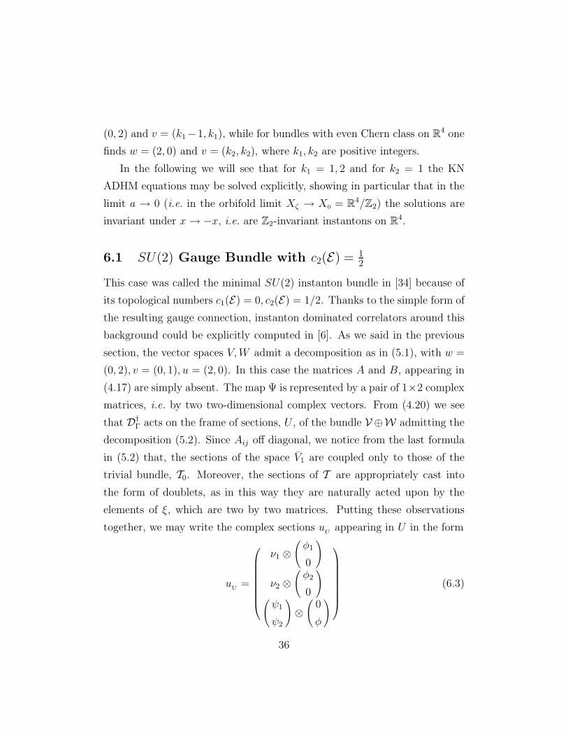
together, we may write the complex sections uU

appearing in U in the form

uU

=

ν1 ⊗(φ1

0

)

ν2 ⊗(φ2

0

)

(ψ1

ψ2

)⊗(

0

φ

)

(6.3)

36

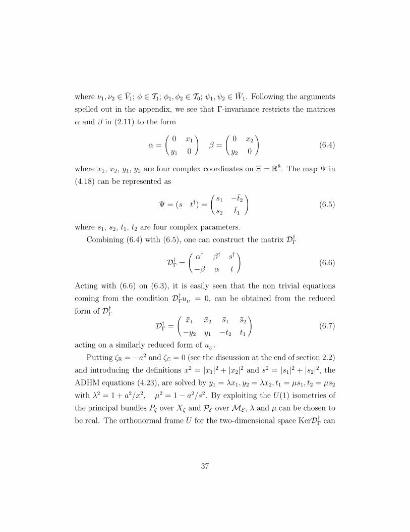
where ν1, ν2 ∈ V1; φ ∈ T1; φ1, φ2 ∈ T0; ψ1, ψ2 ∈ W1. Following the arguments

spelled out in the appendix, we see that Γ-invariance restricts the matrices

α and β in (2.11) to the form

α =

(0 x1

y1 0

)β =

(0 x2

y2 0

)(6.4)

where x1, x2, y1, y2 are four complex coordinates on Ξ = R8. The map Ψ in

(4.18) can be represented as

Ψ = (s t†) =

(s1 −t2s2 t1

)(6.5)

where s1, s2, t1, t2 are four complex parameters.

Combining (6.4) with (6.5), one can construct the matrix D†Γ

D†Γ =

(α† β† s†

−β α t

)(6.6)

Acting with (6.6) on (6.3), it is easily seen that the non trivial equations

coming from the condition D†ΓuU = 0, can be obtained from the reduced

form of D†Γ

D†Γ =

(x1 x2 s1 s2

−y2 y1 −t2 t1

)(6.7)

acting on a similarly reduced form of uU.

Putting ζR = −a2 and ζC = 0 (see the discussion at the end of section 2.2)

and introducing the definitions x2 = |x1|2 + |x2|2 and s2 = |s1|2 + |s2|2, the

ADHM equations (4.23), are solved by y1 = λx1, y2 = λx2, t1 = µs1, t2 = µs2

with λ2 = 1 + a2/x2, µ2 = 1 − a2/s2. By exploiting the U(1) isometries of

the principal bundles Pζ over Xζ and PE over ME , λ and µ can be chosen to

be real. The orthonormal frame U for the two-dimensional space KerD†Γ can

37

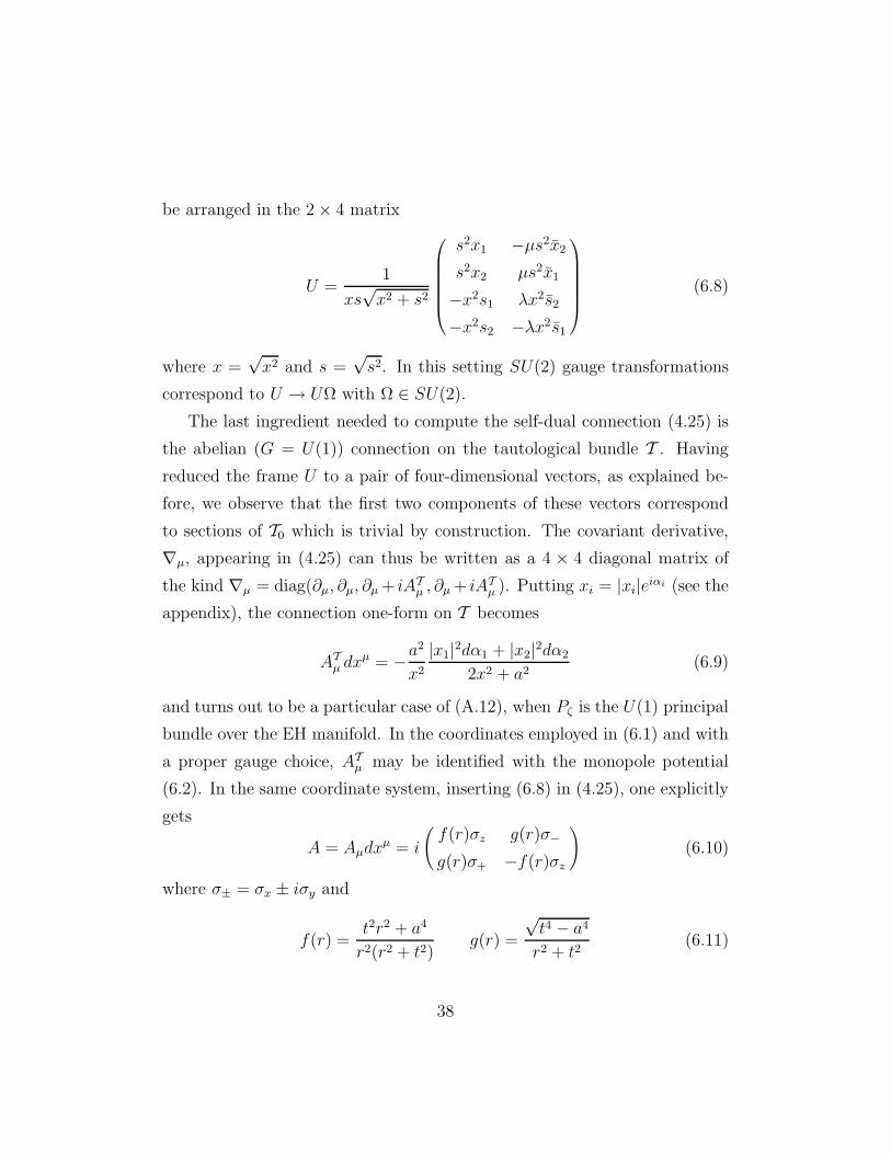
be arranged in the 2 × 4 matrix

U =1

xs√x2 + s2

s2x1 −µs2x2

s2x2 µs2x1

−x2s1 λx2s2

−x2s2 −λx2s1

(6.8)

where x =√x2 and s =

√s2. In this setting SU(2) gauge transformations

correspond to U → UΩ with Ω ∈ SU(2).

The last ingredient needed to compute the self-dual connection (4.25) is

the abelian (G = U(1)) connection on the tautological bundle T . Having

reduced the frame U to a pair of four-dimensional vectors, as explained be-

fore, we observe that the first two components of these vectors correspond

to sections of T0 which is trivial by construction. The covariant derivative,

∇µ, appearing in (4.25) can thus be written as a 4 × 4 diagonal matrix of

the kind ∇µ = diag(∂µ, ∂µ, ∂µ + iATµ , ∂µ + iAT

µ ). Putting xi = |xi|eiαi (see the

appendix), the connection one-form on T becomes

ATµ dx

µ = −a2

x2

|x1|2dα1 + |x2|2dα2

2x2 + a2(6.9)

and turns out to be a particular case of (A.12), when Pζ is the U(1) principal

bundle over the EH manifold. In the coordinates employed in (6.1) and with

a proper gauge choice, ATµ may be identified with the monopole potential

(6.2). In the same coordinate system, inserting (6.8) in (4.25), one explicitly

gets

A = Aµdxµ = i

(f(r)σz g(r)σ−

g(r)σ+ −f(r)σz

)(6.10)

where σ± = σx ± iσy and

f(r) =t2r2 + a4

r2(r2 + t2)g(r) =

√t4 − a4

r2 + t2(6.11)

38

with t2 = 2s2 − a2 and r2 = 2x2 + a2. The resulting self-dual field strength

is given by

F = i

(H(rdr ∧ σz + r2σx ∧ σy) G( r2

udr ∧ σ− + urσ+ ∧ σz)

G( r2

udr ∧ σ+ + urσ− ∧ σz) −H(rdr ∧ σz + r2σx ∧ σy)

)(6.12)

with

H =2

r

df

dr=

4(t2r4 + 2a4r2 + a4t2)

r4(r2 + t2)2

G =2u

r2

dg

dr=

4u√t4 − a4

r(r2 + t2)2(6.13)

Using (6.12), the second Chern class may be checked to be 1/2, as expected.

The connection (6.10) was previously found in [7] following a completely

different procedure. In the limit a → 0 (6.10) becomes a connection over

R4/Z2 and coincides with the BPST instanton (in the singular gauge) with

center located at x0 = 0 and size t [13]. This is no surprise since, in this limit,

this construction gives the usual ADHM construction for SO(3) bundles [30].

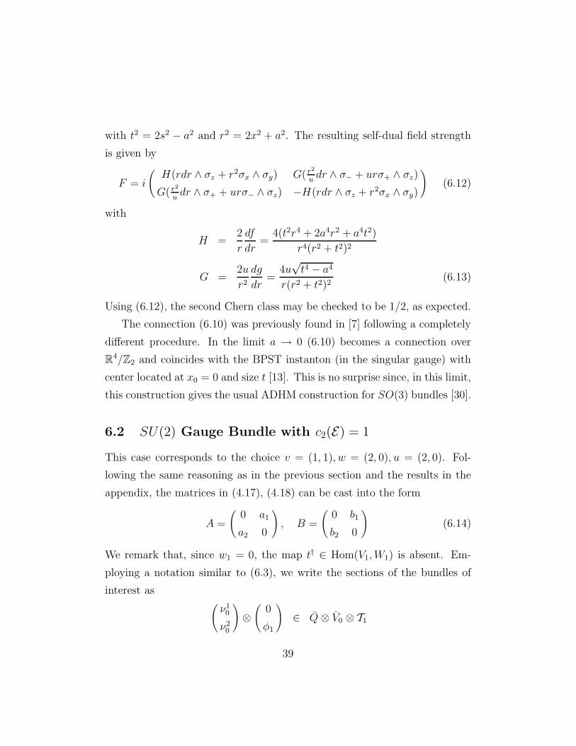
6.2 SU(2) Gauge Bundle with c2(E) = 1

This case corresponds to the choice v = (1, 1), w = (2, 0), u = (2, 0). Fol-

lowing the same reasoning as in the previous section and the results in the

appendix, the matrices in (4.17), (4.18) can be cast into the form

A =

(0 a1

a2 0

), B =

(0 b1

b2 0

)(6.14)

We remark that, since w1 = 0, the map t† ∈ Hom(V1,W1) is absent. Em-

ploying a notation similar to (6.3), we write the sections of the bundles of

interest as(ν1

0

ν20

)⊗(

0

φ1

)∈ Q⊗ V0 ⊗ T1

39

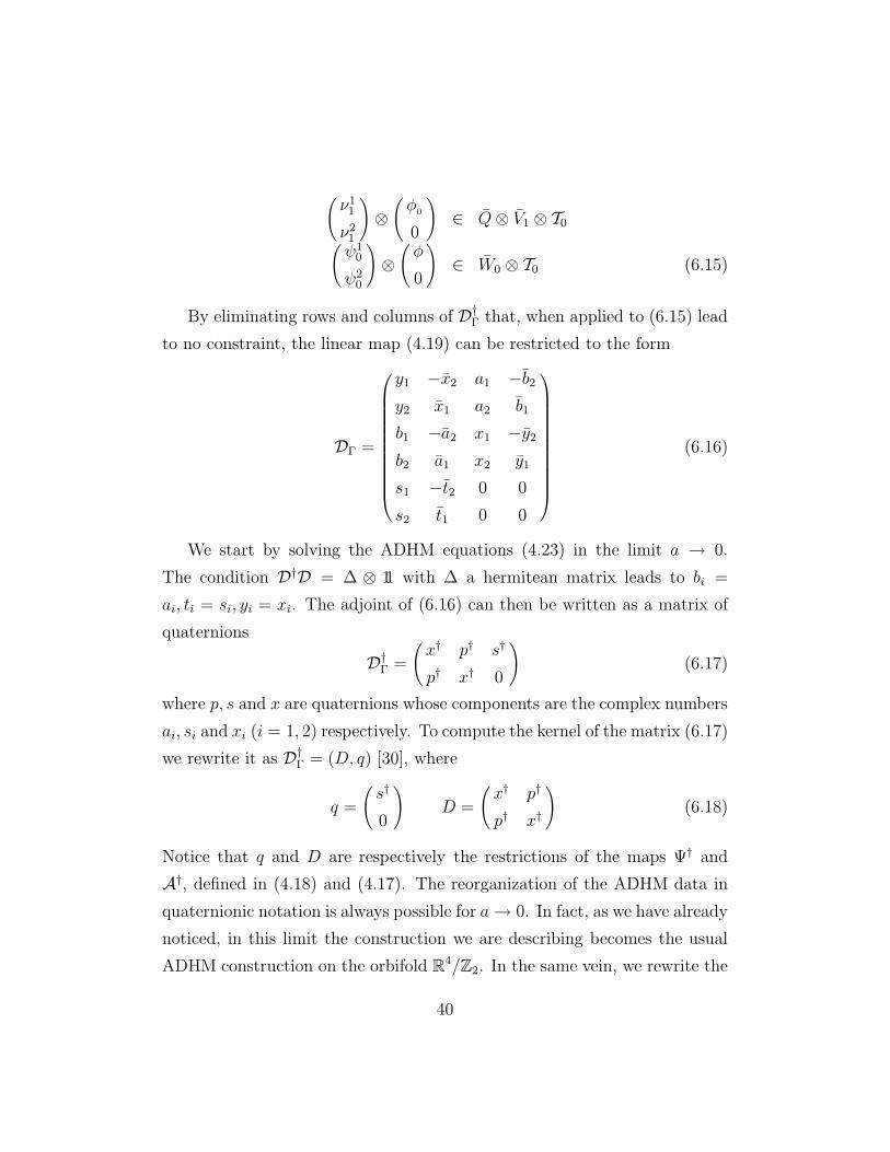
(ν1

1

ν21

)⊗(φ

0

0

)∈ Q⊗ V1 ⊗ T0

(ψ1

0

ψ20

)⊗(φ

0

)∈ W0 ⊗ T0 (6.15)

By eliminating rows and columns of D†Γ that, when applied to (6.15) lead

to no constraint, the linear map (4.19) can be restricted to the form

DΓ =

y1 −x2 a1 −b2y2 x1 a2 b1

b1 −a2 x1 −y2

b2 a1 x2 y1

s1 −t2 0 0

s2 t1 0 0

(6.16)

We start by solving the ADHM equations (4.23) in the limit a → 0.

The condition D†D = ∆ ⊗ 11 with ∆ a hermitean matrix leads to bi =

ai, ti = si, yi = xi. The adjoint of (6.16) can then be written as a matrix of

quaternions

D†Γ =

(x† p† s†

p† x† 0

)(6.17)

where p, s and x are quaternions whose components are the complex numbers

ai, si and xi (i = 1, 2) respectively. To compute the kernel of the matrix (6.17)

we rewrite it as D†Γ = (D, q) [30], where

q =

(s†

0

)D =

(x† p†

p† x†

)(6.18)

Notice that q and D are respectively the restrictions of the maps Ψ† and

A†, defined in (4.18) and (4.17). The reorganization of the ADHM data in

quaternionic notation is always possible for a→ 0. In fact, as we have already

noticed, in this limit the construction we are describing becomes the usual

ADHM construction on the orbifold R4/Z2. In the same vein, we rewrite the

40

frame U in (4.25) as U =

(ν

ϑ

), so that the matrix q (D) will be acting on

the quaternion ϑ (ν).

The condition D†ΓU = 0 yields

ν = −D−1qϑ (6.19)

and U =

(−D−1qϑ

ϑ

). The unitarity constraint U †U = 11 then gives

ϑ =1

√1 + q†(DD†)−1q

ϑ (6.20)

with ϑ†ϑ = 11. By an SU(2) gauge transformation one can always set ϑ = 11.

Exploiting this freedom, (4.25) can be written in the form

Aµ =1

2ϑ2[(D−1q)†∂µ(D−1q) − (∂µ(D−1q)†)(D−1q)] (6.21)

The only delicate point in these formulae is the computation of the matrix

D−1 with the property D−1D = 1. As D is a matrix of quaternions D

does not commute with D−1. The left and the right inverse of D are not

necessarily equal. To compute the left inverse, D−1, we observe that it is

always possible to find matrices Ek such that Ek . . . E2E1D = 11 [35]. Ek is a

matrix representing one of the three possible elementary operations on rows

i) P: permutation of two rows

ii) A: addition of two rows

iii) M: multiplication of a row by a number

A matrix can be diagonalized by a finite number of P, A, M operations.

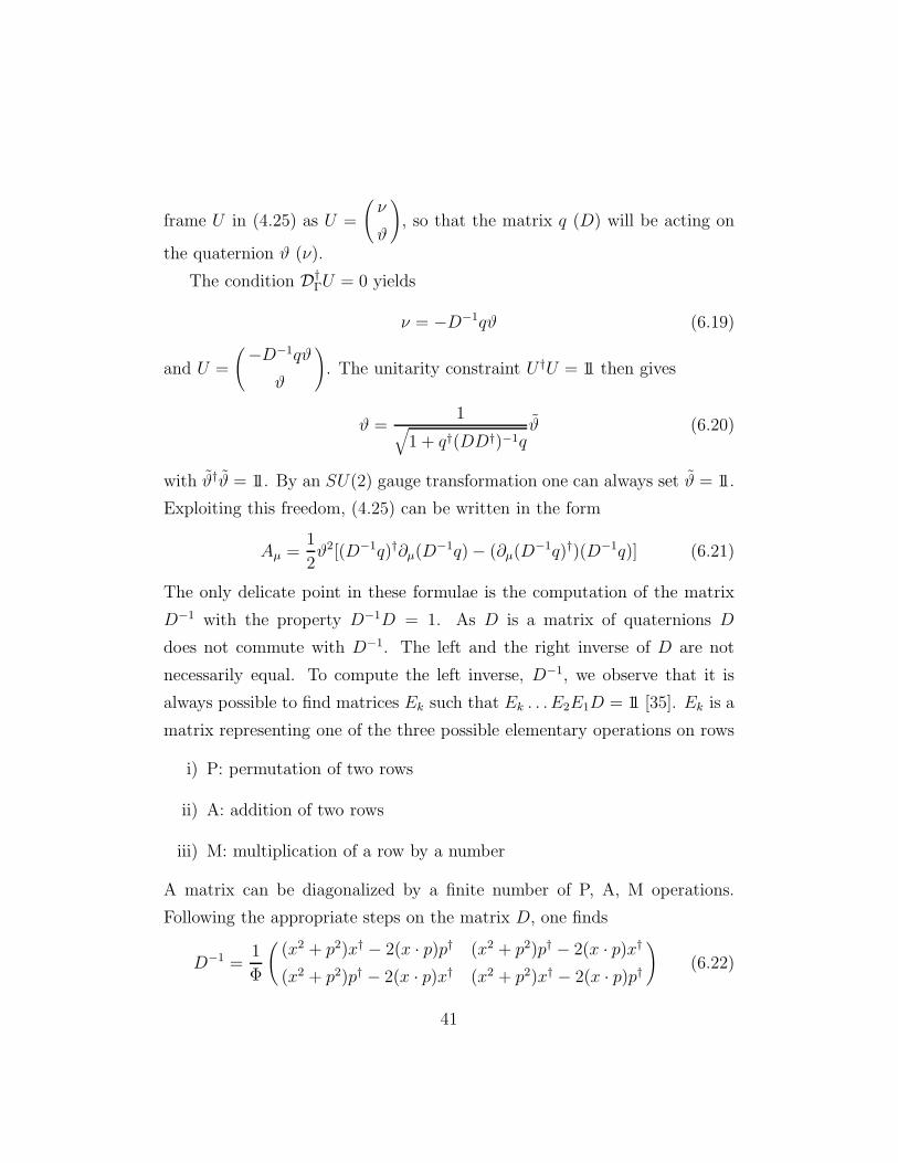
Following the appropriate steps on the matrix D, one finds

D−1 =1

Φ

((x2 + p2)x† − 2(x · p)p† (x2 + p2)p† − 2(x · p)x†

(x2 + p2)p† − 2(x · p)x† (x2 + p2)x† − 2(x · p)p†)

(6.22)

41

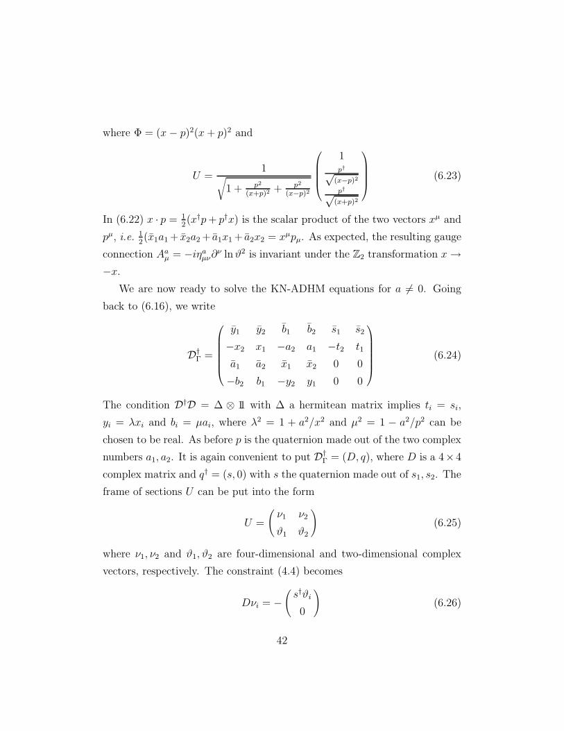
where Φ = (x− p)2(x+ p)2 and

U =1

√1 + p2

(x+p)2+ p2

(x−p)2

1p†√

(x−p)2

p†√(x+p)2

(6.23)

In (6.22) x · p = 12(x†p+ p†x) is the scalar product of the two vectors xµ and

pµ, i.e. 12(x1a1 + x2a2 + a1x1 + a2x2 = xµpµ. As expected, the resulting gauge

connection Aaµ = −iηa

µν∂ν lnϑ2 is invariant under the Z2 transformation x→

−x.We are now ready to solve the KN-ADHM equations for a 6= 0. Going

back to (6.16), we write

D†Γ =

y1 y2 b1 b2 s1 s2

−x2 x1 −a2 a1 −t2 t1

a1 a2 x1 x2 0 0

−b2 b1 −y2 y1 0 0

(6.24)

The condition D†D = ∆ ⊗ 11 with ∆ a hermitean matrix implies ti = si,

yi = λxi and bi = µai, where λ2 = 1 + a2/x2 and µ2 = 1 − a2/p2 can be

chosen to be real. As before p is the quaternion made out of the two complex

numbers a1, a2. It is again convenient to put D†Γ = (D, q), where D is a 4×4

complex matrix and q† = (s, 0) with s the quaternion made out of s1, s2. The

frame of sections U can be put into the form

U =

(ν1 ν2

ϑ1 ϑ2

)(6.25)

where ν1, ν2 and ϑ1, ϑ2 are four-dimensional and two-dimensional complex

vectors, respectively. The constraint (4.4) becomes

Dνi = −(s†ϑi

0

)(6.26)

42

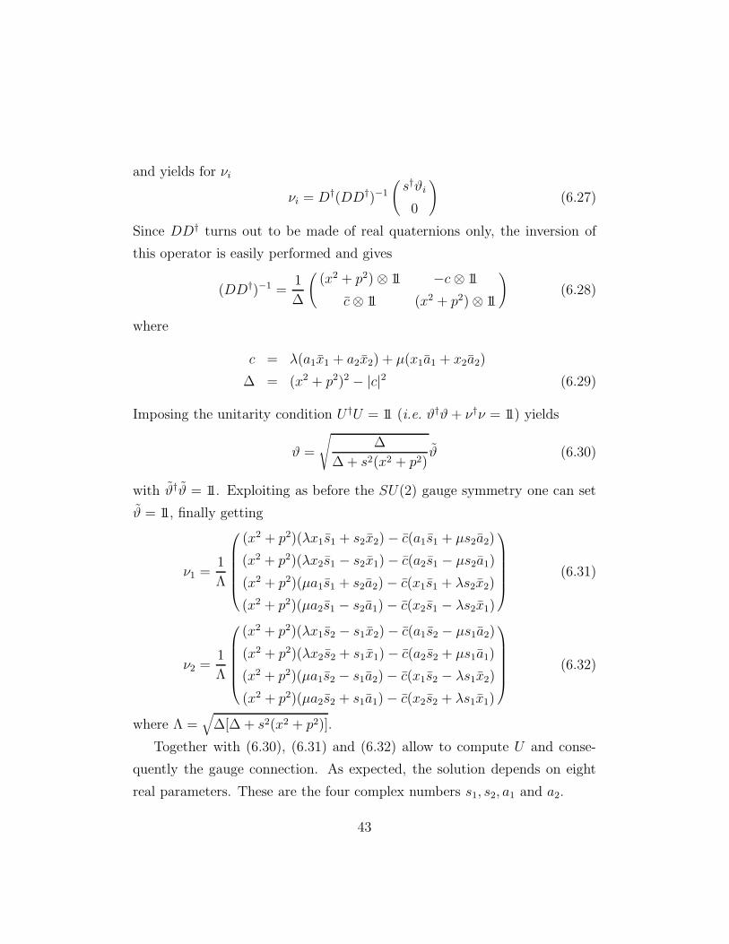
and yields for νi

νi = D†(DD†)−1

(s†ϑi

0

)(6.27)

Since DD† turns out to be made of real quaternions only, the inversion of

this operator is easily performed and gives

(DD†)−1 =1

∆

((x2 + p2) ⊗ 11 −c⊗ 11

c⊗ 11 (x2 + p2) ⊗ 11

)(6.28)

where

c = λ(a1x1 + a2x2) + µ(x1a1 + x2a2)

∆ = (x2 + p2)2 − |c|2 (6.29)

Imposing the unitarity condition U †U = 11 (i.e. ϑ†ϑ+ ν†ν = 11) yields

ϑ =

√∆

∆ + s2(x2 + p2)ϑ (6.30)

with ϑ†ϑ = 11. Exploiting as before the SU(2) gauge symmetry one can set

ϑ = 11, finally getting

ν1 =1

Λ

(x2 + p2)(λx1s1 + s2x2) − c(a1s1 + µs2a2)

(x2 + p2)(λx2s1 − s2x1) − c(a2s1 − µs2a1)

(x2 + p2)(µa1s1 + s2a2) − c(x1s1 + λs2x2)

(x2 + p2)(µa2s1 − s2a1) − c(x2s1 − λs2x1)

(6.31)

ν2 =1

Λ

(x2 + p2)(λx1s2 − s1x2) − c(a1s2 − µs1a2)

(x2 + p2)(λx2s2 + s1x1) − c(a2s2 + µs1a1)

(x2 + p2)(µa1s2 − s1a2) − c(x1s2 − λs1x2)

(x2 + p2)(µa2s2 + s1a1) − c(x2s2 + λs1x1)

(6.32)

where Λ =√

∆[∆ + s2(x2 + p2)].

Together with (6.30), (6.31) and (6.32) allow to compute U and conse-

quently the gauge connection. As expected, the solution depends on eight

real parameters. These are the four complex numbers s1, s2, a1 and a2.

43

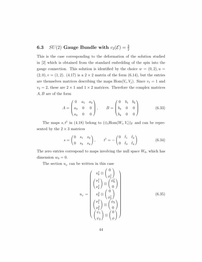
6.3 SU(2) Gauge Bundle with c2(E) = 32

This is the case corresponding to the deformation of the solution studied

in [2] which is obtained from the standard embedding of the spin into the

gauge connection. This solution is identified by the choice w = (0, 2), u =

(2, 0), v = (1, 2). (4.17) is a 2 × 2 matrix of the form (6.14), but the entries

are themselves matrices describing the maps Hom(Vi, Vj). Since v1 = 1 and

v2 = 2, these are 2 × 1 and 1 × 2 matrices. Therefore the complex matrices

A,B are of the form

A =

0 a1 a2

a3 0 0

a4 0 0

, B =

0 b1 b2

b3 0 0

b4 0 0

(6.33)

The maps s, t† in (4.18) belong to (⊕iHom(Wi, Vi))Γ and can be repre-

sented by the 2 × 3 matrices

s =

(0 s1 s2

0 s3 s4

), t† = −

(0 t1 t2

0 t3 t4

)(6.34)

The zero entries correspond to maps involving the null space W0, which has

dimension w0 = 0.

The section uU

can be written in this case

uU

=

ν10 ⊗

(0

φ11

)

(ν1

1

ν12

)⊗(φ1

0

0

)

ν20 ⊗

(0

φ12

)

(ν2

1

ν22

)⊗(φ2

0

)

(ψ1

ψ2

)⊗(

0

φ

)

(6.35)

44

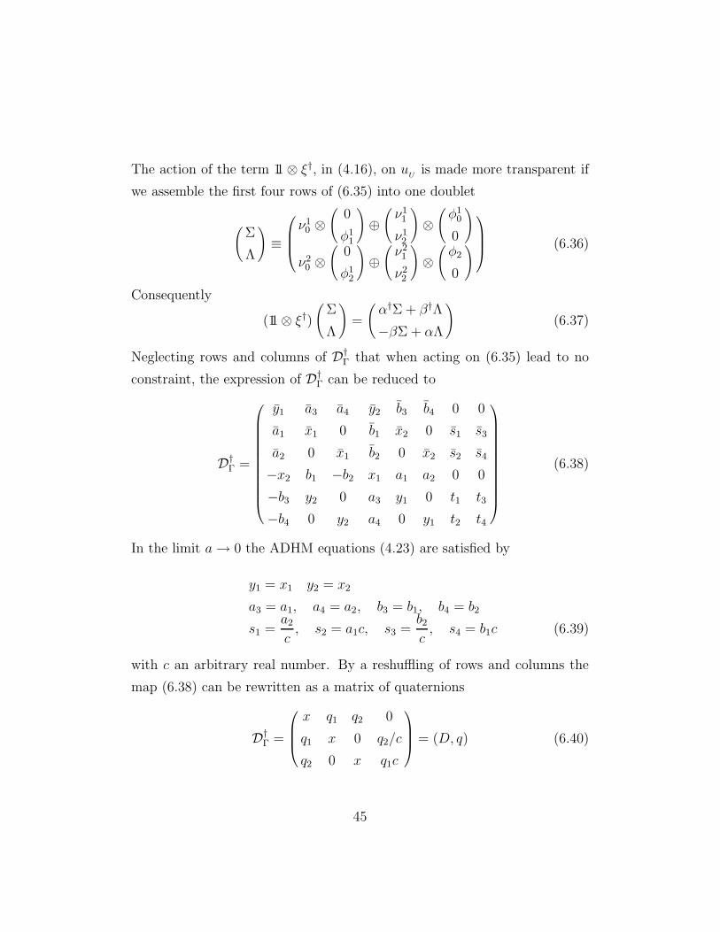
The action of the term 11 ⊗ ξ†, in (4.16), on uU

is made more transparent if

we assemble the first four rows of (6.35) into one doublet

(Σ

Λ

)≡

ν10 ⊗

(0

φ11

)⊕(ν1

1

ν12

)⊗(φ1

0

0

)

ν20 ⊗

(0

φ12

)⊕(ν2

1

ν22

)⊗(φ2

0

)

(6.36)

Consequently

(11 ⊗ ξ†)

(Σ

Λ

)=

(α†Σ + β†Λ

−βΣ + αΛ

)(6.37)

Neglecting rows and columns of D†Γ that when acting on (6.35) lead to no

constraint, the expression of D†Γ can be reduced to

D†Γ =

y1 a3 a4 y2 b3 b4 0 0

a1 x1 0 b1 x2 0 s1 s3

a2 0 x1 b2 0 x2 s2 s4

−x2 b1 −b2 x1 a1 a2 0 0

−b3 y2 0 a3 y1 0 t1 t3

−b4 0 y2 a4 0 y1 t2 t4

(6.38)

In the limit a→ 0 the ADHM equations (4.23) are satisfied by

y1 = x1 y2 = x2

a3 = a1, a4 = a2, b3 = b1, b4 = b2

s1 =a2

c, s2 = a1c, s3 =

b2c, s4 = b1c (6.39)

with c an arbitrary real number. By a reshuffling of rows and columns the

map (6.38) can be rewritten as a matrix of quaternions

D†Γ =

x q1 q2 0

q1 x 0 q2/c

q2 0 x q1c

= (D, q) (6.40)

45

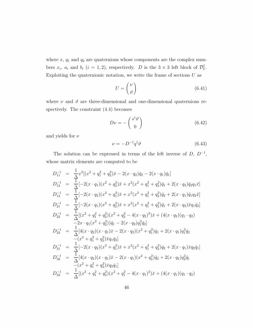
where x, q1 and q2 are quaternions whose components are the complex num-

bers xi, ai and bi (i = 1, 2), respectively. D is the 3 × 3 left block of D†Γ.

Exploiting the quaternionic notation, we write the frame of sections U as

U =

(ν

ϑ

)(6.41)

where ν and ϑ are three-dimensional and one-dimensional quaternions re-

spectively. The constraint (4.4) becomes

Dν = −(s†ϑ

0

)(6.42)

and yields for ν

ν = −D−1q†ϑ (6.43)

The solution can be expressed in terms of the left inverse of D, D−1,

whose matrix elements are computed to be

D−111 =

1

∆x2[(x2 + q2

1 + q22)x− 2(x · q2)q2 − 2(x · q1)q1]

D−112 =

1

∆[−2(x · q1)(x2 + q2

2)x+ x2(x2 + q21 + q2

2)q1 + 2(x · q2)q2q1x]

D−113 =

1

∆[−2(x · q2)(x2 + q2

1)x+ x2(x2 + q21 + q2

2)q2 + 2(x · q1)q1q2x]

D−121 =

1

∆[−2(x · q1)(x2 + q2

2)x+ x2(x2 + q21 + q2

2)q1 + 2(x · q2)xq1q2]

D−122 =

1

∆[(x2 + q2

1 + q22)(x

2 + q22 − 4(x · q2)2)x+ (4(x · q2)(q1 · q2)

−2x · q1(x2 + q22))q1 − 2(x · q2)q2

1 q2]

D−123 =

1

∆[4(x · q2)(x · q1)x− 2(x · q2)(x2 + q2

1)q1 + 2(x · q1)q21 q2

−(x2 + q21 + q2

2)xq1q2]

D−131 =

1

∆[−2(x · q2)(x2 + q2

1)x+ x2(x2 + q21 + q2

2)q2 + 2(x · q1)xq2q1]

D−132 =

1

∆[4(x · q2)(x · q1)x− 2(x · q1)(x2 + q2

2)q2 + 2(x · q2)q22 q1

−(x2 + q21 + q2

2)xq2q1]

D−133 =

1

∆[(x2 + q2

1 + q22)(x

2 + q21 − 4(x · q1)2)x+ (4(x · q1)(q1 · q2)

46

−2(x · q2)(x2 + q21))q2 − 2(x · q1)q2

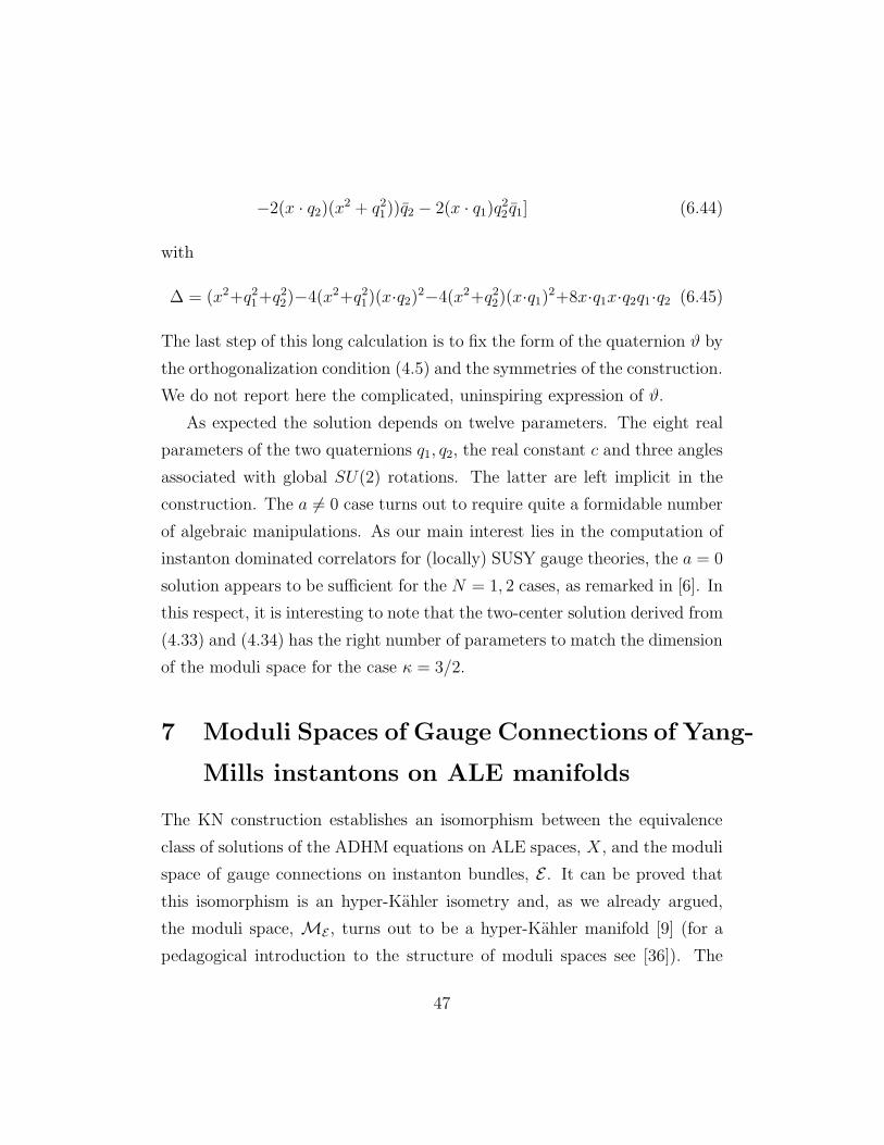
2 q1] (6.44)

with

∆ = (x2+q21+q

22)−4(x2+q2

1)(x·q2)2−4(x2+q22)(x·q1)2+8x·q1x·q2q1·q2 (6.45)

The last step of this long calculation is to fix the form of the quaternion ϑ by

the orthogonalization condition (4.5) and the symmetries of the construction.

We do not report here the complicated, uninspiring expression of ϑ.

As expected the solution depends on twelve parameters. The eight real

parameters of the two quaternions q1, q2, the real constant c and three angles

associated with global SU(2) rotations. The latter are left implicit in the

construction. The a 6= 0 case turns out to require quite a formidable number

of algebraic manipulations. As our main interest lies in the computation of

instanton dominated correlators for (locally) SUSY gauge theories, the a = 0

solution appears to be sufficient for the N = 1, 2 cases, as remarked in [6]. In

this respect, it is interesting to note that the two-center solution derived from

(4.33) and (4.34) has the right number of parameters to match the dimension

of the moduli space for the case κ = 3/2.

7 Moduli Spaces of Gauge Connections of Yang-

Mills instantons on ALE manifolds

The KN construction establishes an isomorphism between the equivalence

class of solutions of the ADHM equations on ALE spaces, X, and the moduli

space of gauge connections on instanton bundles, E . It can be proved that

this isomorphism is an hyper-Kahler isometry and, as we already argued,

the moduli space, ME , turns out to be a hyper-Kahler manifold [9] (for a

pedagogical introduction to the structure of moduli spaces see [36]). The

47

metric G on ME is given by

GIJ =∫

Xd4x

√det(g)gµνδIA

iµδJA

jνδij (7.1)

where g is the metric onX and δA are the zero-mode fluctuations of the gauge

fields around the instanton configuration. The three hyper-Kahler forms on

X can also be mapped into the moduli space, ME , by the formulae

ΩaIJ =

∫

Xd4xωa

µνδIAµi δJA

νj δ

ij (7.2)

The three resulting two-forms, Ωa, are closed and thus define a hyper-Kahler

structure on the moduli space [36].

There is one case in which ME is completely known. To show this we

have to use a very powerful theorem proven in [9, 10], that states that on any

ALE manifold, X, there always exists a bundle, E , with c1(E) = 0, c2(E) =

(|Γ|−1)/|Γ| such that the moduli space, ME is four-dimensional and coincides

with the base manifold X itself. Furthermore there exists a point m0 ∈ ME

at which E(m0) = L ⊕ L with L a line bundle, implying that E is reducible

at m0. While on compact manifolds m0 must be a singular point of the

moduli space [37, 38], this is not necessarily true on non-compact manifolds

[10]. For EH manifold with metric (6.1) r = a is such a point. Going

back to our previous discussion and using this theorem, we see that the

moduli space of connections on the minimal SU(2) instanton (the one with

κ = 1/2) has dimension four (from (5.10)) and precisely coincides with the

EH manifold. Here we have a nice example of symmetry enhancement at a

singular point of a moduli space. As depicted in Fig.2, the EH manifold is

the smooth resolution of the singularity of the orbifold C2/Z2: the parameter

a appearing in (6.1) measures the distance from the singularity. In the limit

a 7→ 0 the SU(2) × U(1) symmetry of the moduli space gets enhanced to

SU(2) × SU(2).

48

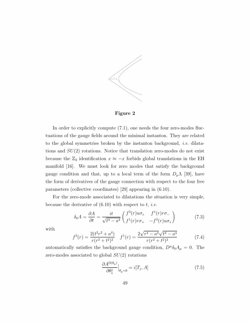
a

Figure 2

In order to explicitly compute (7.1), one needs the four zero-modes fluc-

tuations of the gauge fields around the minimal instanton. They are related

to the global symmetries broken by the instanton background, i.e. dilata-

tions and SU(2) rotations. Notice that translation zero-modes do not exist

because the Z2 identification x ≈ −x forbids global translations in the EH

manifold [16]. We must look for zero modes that satisfy the background

gauge condition and that, up to a local term of the form DµΛ [39], have

the form of derivatives of the gauge connection with respect to the four free

parameters (collective coordinates) [29] appearing in (6.10).

For the zero-mode associated to dilatations the situation is very simple,

because the derivative of (6.10) with respect to t, i.e.

δ0A =∂A

∂t=

it√t4 − a4

(f 3(r)uσz f 1(r)rσ−

f 1(r)rσ+ −f 3(r)uσz

)(7.3)

with

f 3(r) =2(t2r2 + a4)

r(r2 + t2)2f 1(r) =

2√r4 − a4

√t4 − a4

r(r2 + t2)2(7.4)

automatically satisfies the background gauge condition, Dµδ0Aµ = 0. The

zero-modes associated to global SU(2) rotations

∂AΩ(θ0)

∂θj0

∣∣∣θ0=0

= i[Tj , A] (7.5)

49

are not transverse. In order to make them transverse one has to add a local

term of the form DµΛj [39]. Putting Λj = (θj − θ(o)j ), the θj turn out to be

the bounded harmonic scalars given by [34, 6]

θ3 =t2r2 + a4

t2(r2 + t2)θ

(o)3 , θ1,2 =

√r4 − a4

r2 + t2θ

(o)1,2 (7.6)

The resulting three transverse zero-modes have the final expression

δjArµ = (Dµθj)

r (7.7)

The four transverse zero-modes δIA form an orthogonal basis with norms

||δ0A||2 =8π2

g2

t4

t4 − a4

||δ1A||2 = ||δ2A||2 =8π2

g2t2

||δ3A||2 =8π2

g2

t4 − a4

t2(7.8)

where we have introduced back the gauge coupling constant, g.

The framed moduli space of the minimal instanton is four-dimensional

and locally looks like R+ × S3/Z2, with t (t ≥ a) playing the role of the

radial variable. Near the identity element of SU(2) the metric is given by

GIJ =∫

Xd4x

√det(g

EH)gµν

EHδIA

rµδJA

sνδrs (7.9)

The metric GIJ may be transported to any element of the group S3/Z2 by left

translations and one may check that it is identical (up to an overall rescaling)

to the metric in (6.1), after the substitutions

t→ r, exp(iθkTk) → exp(iψT3)exp(iθT2)exp(iφT3) (7.10)

50

8 Conclusions

In this paper we have tackled the problem of the explicit construction of

self-dual gauge connections on ALE manifolds and we have carried out com-

putations for the simplest of all these manifolds the EH gravitational instan-

ton. The results obtained here should allow to generalize the computations

of instanton dominated correlation functions performed in [6]. There we

computed the gaugino condensate in a globally N = 1 supersymmetric YM

theory on the background of the EH manifold by expanding the functional

integral around the minimal SU(2) instanton and we found a constant finite

value as expected on supersymmetry grounds. The explicit calculation of

instanton effects in a supersymmetric YM theory coupled to supergravity

seems to be viable. The relevant Green functions contain a gravitational

sector (represented by the field strength gravitino bilinear) and a gauge sec-

tor (represented by the gaugino bilinears) which are completely decoupled

as argued in [6]. More explicitly, the result of the functional integration in

the gauge sector is independent from the moduli of the gravitational back-

ground, ζC and ζR. This observation suggests that it may suffice to solve the

ADHM equations on ALE spaces in the orbifold limit, ζR = 0, ζC = 0. This,

as we have seen, is a great simplification and it is the reason why we have

presented separately many of the results for the EH background in the limit

a → 0. Unfortunately, even in this limit, the final form of the SU(2) gauge

connection which corresponds to the standard embedding solution, i.e. the

one with c2(E) = 3/2 and dim(ME) = 12, looks quite involved, making the

computation of the relevant zero-modes very complicated. A possible way

out could be to perform these calculations by resorting to the two-center

ansatz (4.33), (4.34).

It is interesting to note that the multi-center ansatz for self-dual SU(2)

gauge connections seems to work for any four-dimensional hyper-Kahler man-

51

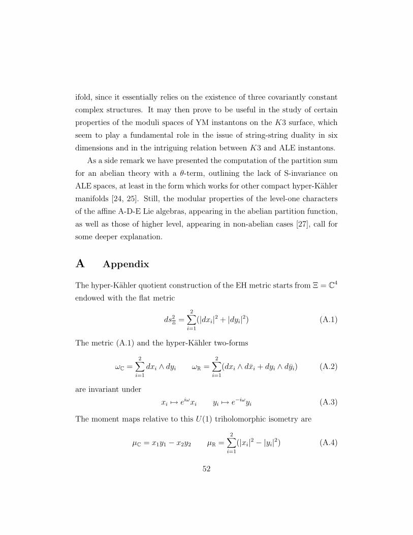
ifold, since it essentially relies on the existence of three covariantly constant

complex structures. It may then prove to be useful in the study of certain

properties of the moduli spaces of YM instantons on the K3 surface, which

seem to play a fundamental role in the issue of string-string duality in six

dimensions and in the intriguing relation between K3 and ALE instantons.

As a side remark we have presented the computation of the partition sum

for an abelian theory with a θ-term, outlining the lack of S-invariance on

ALE spaces, at least in the form which works for other compact hyper-Kahler

manifolds [24, 25]. Still, the modular properties of the level-one characters

of the affine A-D-E Lie algebras, appearing in the abelian partition function,

as well as those of higher level, appearing in non-abelian cases [27], call for

some deeper explanation.

A Appendix

The hyper-Kahler quotient construction of the EH metric starts from Ξ = C4

endowed with the flat metric

ds2Ξ =

2∑

i=1

(|dxi|2 + |dyi|2) (A.1)

The metric (A.1) and the hyper-Kahler two-forms

ωC =2∑

i=1

dxi ∧ dyi ωR =2∑

i=1

(dxi ∧ dxi + dyi ∧ dyi) (A.2)

are invariant under

xi 7→ eiωxi yi 7→ e−iωyi (A.3)

The moment maps relative to this U(1) triholomorphic isometry are

µC = x1y1 − x2y2 µR =2∑

i=1

(|xi|2 − |yi|2) (A.4)

52

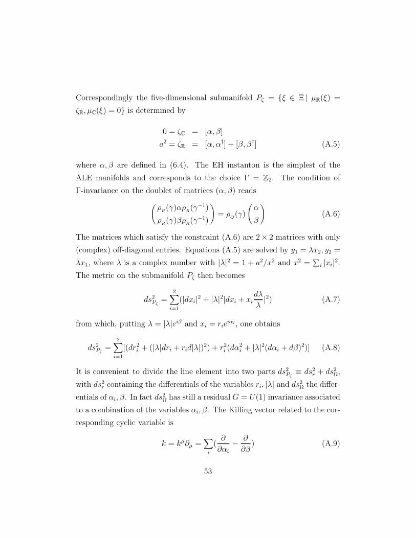
Correspondingly the five-dimensional submanifold Pζ = ξ ∈ Ξ | µR(ξ) =

ζR, µC(ξ) = 0 is determined by

0 = ζC = [α, β]

a2 = ζR = [α, α†] + [β, β†] (A.5)

where α, β are defined in (6.4). The EH instanton is the simplest of the

ALE manifolds and corresponds to the choice Γ = Z2. The condition of

Γ-invariance on the doublet of matrices (α, β) reads

(ρR(γ)αρ

R(γ−1)

ρR(γ)βρ

R(γ−1)

)= ρ

Q(γ)

(α

β

)(A.6)

The matrices which satisfy the constraint (A.6) are 2× 2 matrices with only

(complex) off-diagonal entries. Equations (A.5) are solved by y1 = λx2, y2 =

λx1, where λ is a complex number with |λ|2 = 1 + a2/x2 and x2 =∑

i |xi|2.The metric on the submanifold Pζ then becomes

ds2Pζ

=2∑

i=1

(|dxi|2 + |λ|2|dxi + xidλ

λ|2) (A.7)

from which, putting λ = |λ|eiβ and xi = rieiαi , one obtains

ds2Pζ

=2∑

i=1

[(dr2i + (|λ|dri + rid|λ|)2) + r2

i (dα2i + |λ|2(dαi + dβ)2)] (A.8)

It is convenient to divide the line element into two parts ds2Pζ

≡ ds2r + ds2

Ω,

with ds2r containing the differentials of the variables ri, |λ| and ds2

Ω the differ-

entials of αi, β. In fact ds2Ω has still a residual G = U(1) invariance associated

to a combination of the variables αi, β. The Killing vector related to the cor-

responding cyclic variable is

k = kµ∂µ =∑

i

(∂

∂αi

− ∂

∂β) (A.9)

53

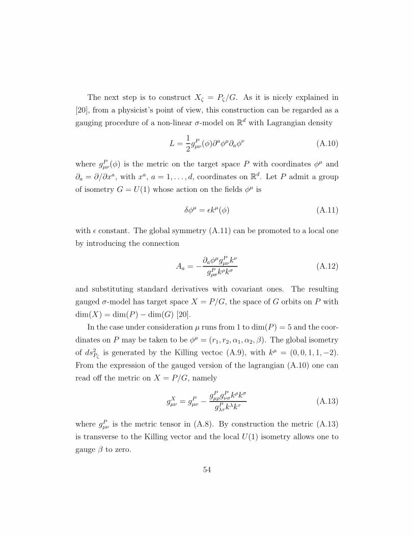
The next step is to construct Xζ = Pζ/G. As it is nicely explained in

[20], from a physicist’s point of view, this construction can be regarded as a

gauging procedure of a non-linear σ-model on Rd with Lagrangian density

L =1

2gP

µν(φ)∂aφµ∂aφν (A.10)

where gPµν(φ) is the metric on the target space P with coordinates φµ and

∂a = ∂/∂xa, with xa, a = 1, . . . , d, coordinates on Rd. Let P admit a group

of isometry G = U(1) whose action on the fields φµ is

δφµ = ǫkµ(φ) (A.11)

with ǫ constant. The global symmetry (A.11) can be promoted to a local one

by introducing the connection

Aa = −∂aφµgP

µνkν

gPρσk

ρkσ(A.12)

and substituting standard derivatives with covariant ones. The resulting

gauged σ-model has target space X = P/G, the space of G orbits on P with

dim(X) = dim(P ) − dim(G) [20].

In the case under consideration µ runs from 1 to dim(P ) = 5 and the coor-

dinates on P may be taken to be φµ = (r1, r2, α1, α2, β). The global isometry

of ds2Pζ

is generated by the Killing vectoc (A.9), with kµ = (0, 0, 1, 1,−2).

From the expression of the gauged version of the lagrangian (A.10) one can

read off the metric on X = P/G, namely

gXµν = gP

µν −gP

µρgPνσk

ρkσ

gPλτk

λkτ(A.13)

where gPµν is the metric tensor in (A.8). By construction the metric (A.13)

is transverse to the Killing vector and the local U(1) isometry allows one to

gauge β to zero.

54

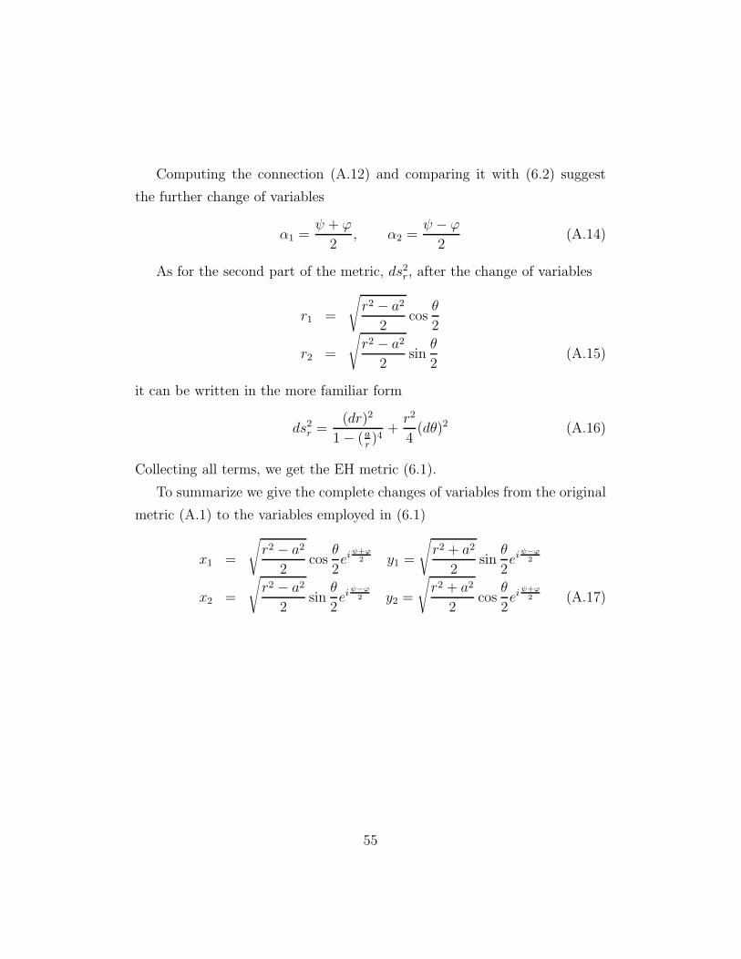
Computing the connection (A.12) and comparing it with (6.2) suggest

the further change of variables

α1 =ψ + ϕ

2, α2 =

ψ − ϕ

2(A.14)

As for the second part of the metric, ds2r, after the change of variables

r1 =

√r2 − a2

2cos

θ

2

r2 =

√r2 − a2

2sin

θ

2(A.15)

it can be written in the more familiar form

ds2r =

(dr)2

1 − (ar)4

+r2

4(dθ)2 (A.16)

Collecting all terms, we get the EH metric (6.1).

To summarize we give the complete changes of variables from the original

metric (A.1) to the variables employed in (6.1)

x1 =

√r2 − a2

2cos

θ

2eiψ+ϕ

2 y1 =

√r2 + a2

2sin

θ

2eiψ−ϕ

2

x2 =

√r2 − a2

2sin

θ

2eiψ−ϕ

2 y2 =

√r2 + a2

2cos

θ

2eiψ+ϕ

2 (A.17)

55

References

[1] T. Eguchi, P.B. Gilkey and A.J. Hanson, Phys. Rep. 66C (1980) 213.

[2] M. Bianchi, F. Fucito, M. Martellini, G.C. Rossi, Nucl. Phys. B440

(1995) 129.

[3] M.G. Duff, R.R. Khuri, J.X. Lu, String Solitons, Phys. Rep. 259C

(1995) 231.

[4] D. Anselmi, M. Billo’, P. Fre’, L. Girardello, A. Zaffaroni, Int. Jou. Mod.

Phys. A9 (1994) 3007.

[5] E. Kiritsis, K. Kounnas and D. Lust, Int. Jou. Mod. Phys. A9 (1994)

1361.

[6] M. Bianchi, F. Fucito, M. Martellini, G.C. Rossi, Phys. Lett. B359

(1995) 56.

[7] H. Boutaleb-Joutei, A. Chakrabarti, A. Comtet, Phys. Rev. D21(1980)

979, ibid. 2285, ibid. 2280.

[8] V. Novikov, M. Shifman, A. Vainshtein and V. Zakharov, Nucl. Phys.

B229 (1983) 381, 407; B260 (1985) 157; G.C. Rossi and G. Veneziano,

Phys. Lett. B138 (1984) 195; I. Affleck, M. Dine and N. Seiberg, Nucl.

Phys. B256 (1985) 557; D. Amati, K. Konishi, Y. Meurice, G.C. Rossi

and G. Veneziano, Phys. Rep. 162C (1988) 169.

[9] P.B. Kronheimer and H. Nakajima, Math. Ann. 288 (1990) 263.

[10] H. Nakajima, Invent. Math. 102 (1990) 267.

[11] T. Gocho and H. Nakajima, J. Math. Soc. Jap. 44 (1992) 43.

56

[12] M. Atiyah, V. Drinfeld, N. Hitchin and Y. Manin, Phys. Lett. 65A

(1978) 185.

[13] M. Atiyah, Geometry of Yang-Mills fields, Lezioni Fermiane, Accademia

Nazionale dei Lincei e Scuola Normale Superiore, Pisa (1979).

[14] N. Hitchin, Math. Proc. Camb. Phil. Soc. 85 (1979) 465.

[15] G. Gibbons, S. Hawking, Phys. Lett. 78B (1978) 430.

[16] T. Eguchi and A.J. Hanson, Ann.Phys.120 (1979) 82.

[17] P.B. Kronheimer, J. Diff. Geom. 29 (1989) 665.

[18] G. ’t Hooft, Phys. Rev. D14 (1976) 3422; erratum, Phys. Rev. D18

(1978) 2199.

[19] R. Jackiw, C. Nohl and C. Rebbi, Phys. Rev. D15 (1977) 1642.

[20] N.J. Hitchin, A. Karlhede, U. Lindstrom and M. Rocek, Comm. Math.

Phys. 108 (1987) 535.

[21] J. McKay, Proc. Sympos. Pure Math., 37 (1980) 183, A.M.S. Providence

R.I.

[22] R. Slanski, Phys. Rep. 79 (1981) 1.

[23] A.L. Yuille, Class. Quant. Grav. 4 (1987) 1409.

[24] E. Verlinde, Nucl. Phys. B455 (1995) 211.

[25] E. Witten, On S-duality in Abelian Gauge Theory, preprint IASSNS-

HEP-95-36, hep-th/9505186.

57

[26] For a review see P. Ginsparg, “Applied Conformal Field Theory”, in

“Fields, Strings and Critical Phenomena”, Les Houches Summer School

1988, North Holland.

[27] C. Vafa, E. Witten, Nucl. Phys. B431 (1994) 3.

[28] A.A. Belavin, A.M. Polyakov, A.S. Schwarz and Yu.S. Tyupkin, Phys.

Lett. 59B (1975) 85.

[29] G. ’t Hooft, unpublished. For a review see A. Actor, Rev. Mod. Phys.

51 (1979) 461.

[30] N. Christ, E. Weinberg, N. Stanton, Phys. Rev. D18 (1978) 2013.

[31] D. Page, Phys. Lett. 85B (1979) 369.

[32] E. Corrigan and P. Goddard, Ann. Phys. 154 (1984) 253.

[33] G. Gibbons, C. Pope and H. Romer, Nucl. Phys. B157 (1979) 377.

[34] M. Bianchi, F. Fucito, M. Martellini, G.C. Rossi, Phys. Lett. B359

(1995) 49.

[35] D. Finkbeiner, Introduction to Matrices and Linear Transformations,

Freeman and Company (1966).

[36] N. Hitchin, Metrics on Moduli Spaces, in Proceedings of the Lefschez

Centennial Conference (Contemporary Math. 58 Part I), A.M.S. Provi-

dence R.I. (1986).

[37] D.S. Freed and K.K. Uhlenbeck, Instantons and Four-Manifolds, MSRI

Publ. 1, Springer-Verlag (1984).

[38] S.K. Donaldson and P.B. Kronheimer, The Geometry of Four-Manifolds,

Oxford University Press (1990).

58

[39] L. Yaffe, Nucl. Phys. B151 (1979) 247; C. Bernard, Phys. Rev. D19

(1979) 3013.

59