The master space of Script N= 1 gauge theories

arX

iv:0

801.

1585

v2 [

hep-

th]

18

Apr

200

8Bicocca-FT-07-17

CERN-PH-TH/2007-266; SISSA 98/2007/EP

Imperial/TP/08/AH/01

NI07096

The Master Space of N = 1 Gauge Theories

Davide Forcella1∗, Amihay Hanany2†, Yang-Hui He3‡, Alberto Zaffaroni4§

1 International School for Advanced Studies (SISSA/ISAS) & INFN-Sezione di Trieste, via Beirut 2, I-34014, Trieste, Italy

PH-TH Division, CERN CH-1211 Geneva 23, Switzerland2 Department of Physics Technion, Israel Institute of Technology Haifa 32000, Israel

Theoretical Physics Group, Blackett Laboratory, Imperial College, London SW7 2AZ, U.K.3 Collegium Mertonense in Academia Oxoniensis, Oxford, OX1 4JD, U.K.

Mathematical Institute, Oxford University, 24-29 St. Giles’, Oxford, OX1 3LB, U.K.

Rudolf Peierls Centre for Theoretical Physics, Oxford University, 1 Keble Road, OX1 3NP, U.K.4 Universita di Milano-Bicocca and INFN, sezione di Milano-Bicocca, Piazza della Scienza, 3; I-20126 Milano, Italy

Abstract

The full moduli space M of a class of N = 1 supersymmetric gauge theories is

studied. For gauge theories living on a stack of D3-branes at Calabi-Yau singularities

X , M is a combination of the mesonic and baryonic branches. In consonance with

the mathematical literature, the single brane moduli space is called the master space

F ♭. Illustrating with a host of explicit examples, we exhibit many algebro-geometric

properties of the master space such as when F ♭ is toric Calabi-Yau, behaviour of its

Hilbert series, its irreducible components and its symmetries. In conjunction with the

plethystic programme, we investigate the counting of BPS gauge invariants, baryonic

and mesonic, using the geometry of F ♭ and show how its refined Hilbert series not only

engenders the generating functions for the counting but also beautifully encode “hid-

den” global symmetries of the gauge theory which manifest themselves as symmetries

of the complete moduli space M for N number of branes.

∗[email protected]†[email protected], [email protected]‡[email protected]§[email protected]

1

http://arXiv.org/abs/0801.1585v2

Contents

1 Introduction 4

2 The Master Space 7

2.1 Warm-up: An Etude in F ♭ . . . . . . . . . . . . . . . . . . . . . . . . . . . . 8

2.1.1 Direct Computation . . . . . . . . . . . . . . . . . . . . . . . . . . . 9

2.1.2 Hilbert Series . . . . . . . . . . . . . . . . . . . . . . . . . . . . . . . 10

2.1.3 Irreducible Components and Primary Decomposition . . . . . . . . . 11

2.1.4 Toric Presentation: Binomial Ideals and Toric Ideals . . . . . . . . . 14

2.1.5 Computing the Refined Hilbert Series . . . . . . . . . . . . . . . . . . 17

2.1.6 The Symplectic Quotient Description . . . . . . . . . . . . . . . . . . 18

2.1.7 Dimer Models and Perfect Matchings . . . . . . . . . . . . . . . . . . 21

2.2 Case Studies . . . . . . . . . . . . . . . . . . . . . . . . . . . . . . . . . . . . 25

2.2.1 The Suspended Pinched Point. . . . . . . . . . . . . . . . . . . . . . . 26

2.2.2 Cone over Zeroth Hirzebruch Surface . . . . . . . . . . . . . . . . . . 28

2.2.3 Cone over First del Pezzo Surface: dP1 . . . . . . . . . . . . . . . . . 32

2.2.4 Cone over Second del Pezzo Surface: dP2 . . . . . . . . . . . . . . . . 34

2.2.5 Cone over Third del Pezzo Surface: dP3 . . . . . . . . . . . . . . . . 36

2.2.6 Cone over Fourth Pseudo del Pezzo Surface: PdP4 . . . . . . . . . . . 38

2.2.7 Cone over Fifth Pseudo del Pezzo Surface: PdP5 . . . . . . . . . . . . 40

2.3 The Master Space: Recapitulation . . . . . . . . . . . . . . . . . . . . . . . . 42

2.3.1 The Toric N = 1 Case . . . . . . . . . . . . . . . . . . . . . . . . . . 43

2.3.2 General N . . . . . . . . . . . . . . . . . . . . . . . . . . . . . . . . . 46

2.3.3 The Plethystic Programme Reviewed . . . . . . . . . . . . . . . . . . 47

2

3 Linear Branches of Moduli Spaces 49

3.1 The (C2/Z2) × C Singularity . . . . . . . . . . . . . . . . . . . . . . . . . . . 50

3.2 Case Studies Re-examined . . . . . . . . . . . . . . . . . . . . . . . . . . . . 51

3.2.1 Multiple Flows . . . . . . . . . . . . . . . . . . . . . . . . . . . . . . 53

4 Hidden Global Symmetries 55

4.1 Character Expansion: A Warm-up with C3 . . . . . . . . . . . . . . . . . . . 56

4.2 Conifold Revisited . . . . . . . . . . . . . . . . . . . . . . . . . . . . . . . . 58

4.2.1 Hidden Symmetries for Higher Plethystics . . . . . . . . . . . . . . . 60

4.3 F0 Revisited . . . . . . . . . . . . . . . . . . . . . . . . . . . . . . . . . . . . 62

4.4 dP0 Revisited . . . . . . . . . . . . . . . . . . . . . . . . . . . . . . . . . . . 64

4.4.1 Higher Number of Branes . . . . . . . . . . . . . . . . . . . . . . . . 66

4.5 dP1 Revisited . . . . . . . . . . . . . . . . . . . . . . . . . . . . . . . . . . . 68

4.6 dP2 Revisited . . . . . . . . . . . . . . . . . . . . . . . . . . . . . . . . . . . 69

4.7 dP3 Revisited . . . . . . . . . . . . . . . . . . . . . . . . . . . . . . . . . . . 70

4.8 A Prediction for True dP4 . . . . . . . . . . . . . . . . . . . . . . . . . . . . 72

5 Conclusions and Prospectus 74

A Hilbert Series of Second Kind and the Reeb Vector 78

B Refined Hilbert Series: Macaulay2 Implementation 79

C Refined Hilbert Series using Molien Formula 80

3

1 Introduction

The vacuum moduli space, M, of supersymmetric gauge theories is one of the most fun-

damental quantities in modern physics. It is given by the vanishing of the scalar potential

as a function of the scalar components of the superfields of the field theory. This, in turn,

is the set of zeros, dubbed flatness, of so-called D-terms and F-terms, constituting a pa-

rameter, or moduli, space of solutions describing the vacuum. The structure of this space

is usually complicated, and should be best cast in the language of algebraic varieties. Typi-

cally, M consists of a union of various branches, such as the mesonic branch or the baryonic

branch, the Coulomb branch or the Higgs branch; the names are chosen according to some

characteristic property of the specific branch.

It is a standard fact now that M can be phrased in a succinct mathematical language:

it is the symplectic quotient of the space of F-flatness, by the gauge symmetries provided by

the D-flatness. We will denote the space of F-flatness by F ♭ and symmetries prescribed by

D-flatness as GD♭, then we have

M ≃ F ♭//GD♭ . (1.1)

Using this language, we see that F ♭ is a parent space whose quotient is a moduli space. In

the mathematical literature, this parent is referred to as the master space [1] and to this

cognomen we shall adhere1.

In the context of certain string theory backgrounds, M has an elegant geometrical

realisation. When D-branes are transverse to an affine (non-compact) Calabi-Yau space X ,

a supersymmetric gauge theory exists on the world-volume of the branes. Of particular

interest is, of course, when the gauge theory, prescribed by D3-branes, is in four-dimensions.

Our main interest is the IR physics of this system, where all Abelian symmetry decouples

and the gauge symmetry is fully non-Abelian, typically given by products of SU(N) groups.

The Abelian factors are not gauged but rather appear as global baryonic symmetries of the

gauge theory.

Under these circumstances, the moduli space M is a combined mesonic branch and

baryonic branch. These branches are not necessarily separate (irreducible) components of

M but are instead in most cases intrinsically merged into one or more components in M.

Even when mesonic and baryonic directions are mixed, it still makes sense to talk about the

1We thank Alastair King to pointing this out to us.

4

more familiar mesonic moduli space mesM, as the sub-variety of M parameterized by mesonic

operators only. Since mesonic operators have zero baryonic charge, and thus invariant under

the U(1) Abelian factors, the mesonic moduli space can be obtained as a further quotient of

M by the Abelian symmetries:

mesM ≃ M//U(1)D♭ . (1.2)

We are interested in the theory of physical N branes probing the singularity; the gauge

theory on the worldvolume is then superconformal.

It is of particular interest to consider the case of a single D3-brane transverse to the

Calabi-Yau three-fold X , which will enlighten the geometrical interpretation of the moduli

space. Since the motion of the D-brane is parameterized by this transverse space, part of the

vacuum moduli space M is, per constructionem, precisely the space which the brane probes.

The question of which part of the moduli space is going to be clarified in detail in this paper.

For now it is enough to specify that for a single D-brane it is the mesonic branch:

M ⊃ mesM ≃ X ≃ non-compact Calabi-Yau threefold transverse to D3-brane. (1.3)

In this paper we are interested in studying the full moduli space M. In general, Mwill be an algebraic variety of dimension greater than three. In the case of a single D3-brane,

N = 1, the IR theory has no gauge group and the full moduli space M is given by the space

of F-flatness F ♭. Geometrically, F ♭ is a CdimF♭−3 fibration over the mesonic moduli space

X given by relaxing the U(1) D-term constraints in (1.2). Physically, F ♭ is obtained by

adding baryonic directions to the mesonic moduli space. Of course, we can not talk about

baryons for N = 1 but we can alternatively interpret these directions as Fayet-Iliopoulos

(FI) parameters in the stringy realization of the N = 1 gauge theory. Indeed on the world-

volume of a single D-brane there is a collection of U(1) gauge groups, each giving rise to a FI

parameter, which relax the D-term constraint in (1.2). When these FI parameters acquire

vacuum expectation values they induce non-zero values for the collection of fields in the

problem and this is going to be taken to be the full moduli space M ≡ F ♭. If one further

restricts the moduli space to zero baryonic number we get the mesonic branch which is X ,

the Calabi-Yau itself.

For N > 1 number of physical branes, the situation is more subtle. The mesonic moduli

space, probed by a collection of N physical branes, is given by the symmetrized product of

5

N copies of X 2. The full moduli space M is a bigger algebraic variety of more difficult

characterization. One of the purposes of this paper is to elucidate this situation and to show

how the properties of M for arbitrary number of branes are encoded in the master space F ♭

for a single brane. In view of the importance of the master space F ♭ for one brane even for

larger N , we will adopt the important convention that, in the rest of the paper, the word

master space and the symbol F ♭ will refer to the N = 1 case, unless explicitly stated.

The symplectic quotient structure of (1.1) should immediately suggest toric varieties

in the N = 1 case. Indeed, the case of X being a toric Calabi-Yau space has been studied

extensively over the last decade. The translation between the physics data of the D-brane

world volume gauge theory and the mathematical data of the geometry of the toric X was

initiated in [3, 4, 5]. In the computational language of [5], the process of arriving at the

toric diagram from the quiver diagram plus superpotential was called the forward algorithm,

whereas the geometrical computation of the gauge theory data given the toric diagram was

called the inverse algorithm. The computational intensity of these algorithms, bottle-necked

by finding dual integer cones, has been a technical hurdle.

Only lately it is realized that the correct way to think about toric geometry in the

context of gauge theories is through the language of dimer models and brane tilings [6, 7].

Though the efficiency of this new perspective has far superseded the traditional approach of

the partial resolutions of the inverse algorithm, the canonical toric language of the latter is

still conducive to us, particularly in studying objects beyond X , and in particular, F ♭. We

will thus make extensive use of this language as well as the modern one of dimers.

Recently, a so-called plethystic programme [9, 10, 11, 12, 13] has been advocated

in counting the gauge invariant operators of supersymmetric gauge theories, especially in

the above-mentioned D-brane quiver theories. For mesonic BPS operators, the fundamental

generating function turns out to be the Hilbert series of X [9]. The beautiful fact is that the

full counting [11], including baryons as well, is achieved with the Hilbert series of F ♭ for one

brane! Indeed, mesons have gauge-index contractions corresponding to closed paths in the

quiver diagram and the quotienting by GD♭ achieves this. Baryons, on the other hand, have

more general index-contractions and correspond to all paths in the quiver; whence their

counting should not involve the quotienting and the master space should determine their

counting.

2Cf. [2] for a consistency analysis of this identification.

6

In light of the discussions thus far presented, it is clear that the master space F ♭ of

gauge theories, especially those arising from toric Calabi-Yau threefolds, is of unquestionable

importance. It is therefore the purpose of this paper to investigate their properties in detail.

We exhibit many algebro-geometric properties of the master space F ♭ for one brane, including

its decomposition into irreducible components, its symmetry and the remarkable property of

the biggest component of being always toric Calabi-Yau if X is. We point out that even

though we mainly concentrate on the master space F ♭ for one brane, we are able, using the

operator counting technique, to extract important information about the complete moduli

space M, information such as its symmetries for arbitrary number of branes.

The organisation of the paper is as follows. In §2 we introduce the concept of the master

space in detail, starting with various computational approaches, emphasizing on the Hilbert

series and toric presentation, and then launching into a wealth of illustrative examples. We

recapitulate at the end of the section on the key abstract properties of the master space

while reviewing the plethystic programme which counts gauge invariants given the Hilbert

series. We then, in §3, discuss how the master space, and indeed, the moduli space of

supersymmetric theories, are generically reducible and have various branches which we will

obtain by primary decomposition. We shall see how certain lower dimensional components

of one theory causes it to flow to another. Another remarkable feature of gauge theories

arising from underlying geometry such as those living on world-volumes of D-brane probes at

Calabi-Yau singularities is that the symmetries of the master space can manifest themselves

as hidden global symmetries of the gauge theory. In §4 we examine how such symmetries

beautifully exhibit themselves in the plethystics of the Hilbert series of the master space by

explicitly arranging themselves into representations of the associated Lie algebra. Finally,

we part with concluding remarks and outlooks in §5.

Due to the length of this paper, we find it expedient to supplement it with a companion

essay [14]. The reader who wishes for a quick tour of the high-lights is referred thereto.

2 The Master Space

It was realized in [4] that for a single D3-brane probing a toric Calabi-Yau threefold X ,

the space of solutions to the F-terms (or, in the notation of Section 1.2 in Cit. Ibid., the

commuting variety Z) is also a toric variety, albeit of higher dimension. In particular, for

7

a quiver theory with g nodes, it is of dimension g + 2. Thus we have the first important

property for the master space F ♭ for a toric U(1)g quiver theory:

dim(F ♭) = g + 2 . (2.1)

This can be seen as follows. The F-term equations are invariant under a (C∗)g+2 action,

given by the three mesonic symmetries of the toric quiver, one R and two flavor symmetries,

as well as the g − 1 baryonic symmetries, including the anomalous ones. This induces an

action of (C∗)g+2 on the master space. Moreover, the dimension of F ♭ is exactly g + 2 as

the following field theory argument shows. We know that the mesonic moduli space has

dimension three, being isomorphic to the transverse Calabi-Yau manifold X . As described

in the introduction, the mesonic moduli space is obtained as the solution of both F-term

and D-term constraints for the U(1)g quiver theory. The full master space is obtained by

relaxing the U(1) D-term constraints. Since an overall U(1) factor is decoupled, we have

g − 1 independent baryonic parameters corresponding to the values of the U(1) D-terms,

which, by abuse of language, we can refer to as FI terms. As a result, the dimension of the

master space is g + 2, given by three mesonic parameters plus g − 1 FI terms.

A second property of the Master Space is its reducibility. We will see in several examples

below that it decomposes into several irreducible components, the largest of which turns out

to be of the same dimension as the master space, and more importantly the largest component

is a toric Calabi-Yau manifold in g +2 complex dimensions which is furthermore a cone over

a Sasaki Einstein manifold of real dimension 2g + 3. Examples follow below, as well as a

proof that it is Calabi-Yau in section §2.3.

Having learned the dimension of the master space, let us now see a few warm-up

examples of what the space looks like. Let us begin with an illustrative example of perhaps

the most common affine toric variety, viz., the Abelian orbifold.

2.1 Warm-up: An Etude in F ♭

The orbifold C3/Zk × Zm is well-studied. It is an affine toric singularity whose toric dia-

grams are lattice points enclosed in a right-triangle of lengths k × m (cf. e.g., [15]). The

matter content and superpotential for these theories can be readily obtained from brane-box

8

constructions [16]. We summarize as follows:

Gauge Group Factors: mn;

Fields: bi-fundamentals{Xi,j, Yi,j, Zi,j} from node i to node j

(i, j) defined modulo (k, m) , total = 3mn;

Superpotential: W =k−1∑

i=0

m−1∑

j=0

Xi,jYi+1,jZi+1,j+1 − YijXi,j+1Zi+1,j+1 .

(2.2)

We point out here the important fact that in the notation above, when either of the factors

(k, m) is equal to 1, the resulting theory is really an N = 2 gauge theory since the action of

Zk ×Zm on the C3 is chosen so that it degenerates to have a line of singularities when either

k or m equals 1. In other words, if m = 1 in (2.2), we would have a (C2/Zk) × C orbifold

rather than a proper C3/Zk one (in the language of [19], this proper action would be called

“transitive”). We shall henceforth be careful to distinguish these two types of orbifolds with

this notation.

2.1.1 Direct Computation

Given the matter content and superpotential of an N = 1 gauge theory, a convenient and

algorithmic method of computation, emphasising (1.1), is that of [20]. We can immediately

compute F ♭ as an affine algebraic variety: it is an ideal in C3mn given by the 3mn equations

prescribed by ∂W = 0. The defining equation is also readily obtained: it is simply the image

of the ring map ∂W from C3mn → C3mn, i.e., the syzygies of the 3mn polynomials given by

∂W . To specify F ♭ explicitly as an affine algebraic variety, let us use the notation that

(d, δ|p) := affine variety of dimension d and degree δ embedded in Cp . (2.3)

Subsequently, we present what F ♭ actually is as an algebraic variety for some low values

of (m, k) in Table 1. We remind the reader that, of course, quotienting these above spaces

by D♭, which in the algorithm of [20] is also achieved by a ring map, should all give our

starting point of X = C3/Zk × Zm.

As pointed out above, the limit of either k or m going to 1 in the theory prescribed in

(2.2) is really just (C2/Zk) × C with the X-fields, say, acting as adjoints. The first row and

column of (1) should thus be interpreted carefully since they are secretly N = 2 theories

with adjoints. We shall study proper C3/Zk theories later.

9

m\k 1 2 3 4 5

1 (3, 1|3) (4, 2|6) (5, 4|9) (6, 8|12) (7, 16|15)

2 (4, 2|6) (6, 14|12) (8, 92|18) (10, 584|24) (12, 3632|30)

3 (5, 4|9) (8, 92|18) (11, 1620|27) (14, 26762|36) (17, 437038|45)

Table 1: The master space F ♭ for C3/Zk ×Zm as explicit algebraic varieties, for some low values

of k and m.

2.1.2 Hilbert Series

One of the most important quantities which characterize an algebraic variety is the Hilbert

series3. In [9], it was pointed out that it is also key to the problem of counting gauge invariant

operators in the quiver gauge theory. Let us thus calculate this quantity for F ♭.

We recall that for a variety M in C[x1, ..., xk], the Hilbert series is the generating

function for the dimension of the graded pieces:

H(t; M) =∞∑

i=−∞

dimC Miti , (2.4)

where Mi, the i-th graded piece of M can be thought of as the number of independent degree

i (Laurent) polynomials on the variety M . The most useful property of H(t) is that it is a

rational function in t and can be written in 2 ways:

H(t; M) =

{Q(t)

(1−t)k , Hilbert series of First Kind ;P (t)

(1−t)dim(M) , Hilbert series of Second Kind .(2.5)

Importantly, both P (t) and Q(t) are polynomials with integer coefficients. The powers of the

denominators are such that the leading pole captures the dimension of the manifold and the

embedding space, respectively. In particular, P (1) always equals the degree of the variety.

We can also relate the Hilbert series to the Reeb vector, which elucidate in Appendix A.

For now, let us present in Table 2 the Hilbert series, in Second form, of some of the

examples above in Table 1. We see that indeed the leading pole is the dimension of F ♭ and

that the numerator evaluated at 1 (i.e., the coefficient of the leading pole) is equal to the

degree of F ♭. Furthermore, we point out that the Hilbert series thus far defined depends on

a single variable t, we shall shortly discuss in §2.1.5 and also from Appendix A how to refine

this to multi-variate and how these variables should be thought of as chemical potentials.

3Note, however, that the Hilbert series is not a topological invariant and does depend on embedding.

10

(k, m) F ♭ Hilbert Series H(t;F ♭)

(2, 2) (6, 14|12) 1+6 t+9 t2−5 t3+3 t4

(1−t)6

(2, 3) (8, 92|18) 1+10 t+37 t2+47 t3−15 t4+7 t5+5 t6

(1−t)8

(2, 4) (10, 584|24) 1+14 t+81 t2+233 t3+263 t4−84 t5+4 t6+71 t7−7 t8+8 t9

(1−t)10

(3, 3) (11, 1620|27) 1+16 t+109 t2+394 t3+715 t4+286 t5−104 t6+253 t7−77 t8+27 t9

(1−t)11

Table 2: The Hilbert series, in second form, of the master space F ♭ for C3/Zk × Zm, for some

low values of k and m.

2.1.3 Irreducible Components and Primary Decomposition

The variety F ♭ may not be a single irreducible piece, but rather, be composed of various

components. This is a well recognized feature in supersymmetric gauge theories. The dif-

ferent components are typically called branches of the moduli space, such as Coulomb

or Higgs branches, mesonic or baryonic branches. Possibly the most famous case is the

Seiberg-Witten solution to N = 2 supersymmetric gauge theories which deals mainly with

the Coulomb branch but gives some attention to the other components on the moduli space

which are generically called the Higgs branch.

It is thus an interesting question to identify the different components since sometimes

the massless spectrum on each component has its own unique features. We are naturally

lead to a process to extract the various components which in the math literature is called

primary decomposition of the ideal corresponding to F ♭. This is an extensively studied

algorithm in computational algebraic geometry (cf. e.g. [21]) and a convenient programme

which calls these routines externally but based on the more familiar Mathematica interface

is [22].

Example of C2/Z3: Let us first exemplify with the case of (C2/Z3) × C (i.e., (k, m) =

(1, 3)). This case, having N = 2 supersymmetry, is known to have a Coulomb branch and a

Higgs branch which is a combined mesonic and baryonic branch. The superpotential is

W(C2/Z3)×C = X0,0 Y0,0 Z0,1−Y0,0 X0,1 Z0,1+X0,1 Y0,1 Z0,2−Y0,1 X0,2 Z0,2+X0,2 Y0,2 Z0,0−Y0,2 X0,0 Z0,0 ,

(2.6)

composed of a total of 9 fields, where the X fields are adjoint fields in the N = 2 vector

multiplet of the corresponding gauge group. Here, since we are dealing with a single D-brane,

11

>>>

2

<<<

<<<

3

1

WC3/Z3= ǫαβγX

(α)12 X

(β)23 X

(γ)31

9 fields and 27 GIO’s

X(α)12 , X

(β)23 , X

(γ)31 , α, β, γ = 1, 2, 3

Figure 1: The quiver diagram and superpotential for dP0.

these fields have charge 0. Hence, F ♭ is defined, as an ideal in C9, by 9 quadrics:

F ♭(C2/Z3)×C

= {−Y0,2 Z0,0 + Y0,0 Z0,1 , −Y0,0 Z0,1 + Y0,1 Z0,2 , Y0,2 Z0,0 − Y0,1 Z0,2 ,

(X0,0 − X0,1) Z0,1 , (X0,1 − X0,2) Z0,2 , (−X0,0 + X0,2) Z0,0 ,

(−X0,0 + X0,2) Y0,2 , (X0,0 − X0,1) Y0,0 , (X0,1 − X0,2) Y0,1} .

(2.7)

Immediately one can see that on one branch, the so-called Higgs branch, which we shall

denote as F ♭1, the adjoint fields X do not participate. Thus it is defined by the first 3

equations in (2.7): 3 quadrics in 6 variables. Furthermore, one can see that one of the

quadrics is not independent. Therefore F ♭1 is a complete intersection of 2 quadratics in C6,

of dimension 4. To this we must form a direct product with the Coulomb branch which is

parametrized by the X-directions, which turns out to be one dimensional X0,0 = X0,1 = X0,2

(in order to satisfy the remaining 6 equations from (2.7) such that the Y ’s and Z’s are non-

zero). Hence, F ♭ is 5-dimensional (as we expect from (2.1) since there are g = 3 nodes), of

degree 4, and composed of 2 quadrics in C6 crossed with C.

Now, this example may essentially be observed with ease, more involved examples

requires an algorithmic approach, as we shall see in many cases which ensue. The decoupling

of the X’s is indicative of the fact that we have an non-transitive action and this is indeed

just an orbifold of C2.

Example of dP0 = C3/Z3: Let us next study a proper orbifold C

3/Z3 with a non-trivial

action, say (1, 1, 1), on the C3. This is also referred to in the literature as dP0, the cone

over the zeroth del Pezzo surface. In other words, this is the total space of the line bundle

OP2(−3) over P2. Here, there are 9 fields and the theory is summarized in Figure 1. Now,

12

the F-terms are

F ♭C3/Z3

= {−X32,3 X2

3,1 + X22,3 X3

3,1 , X32,3 X1

3,1 − X12,3 X3

3,1 , −X22,3 X1

3,1 + X12,3 X2

3,1,

X31,2 X2

3,1 − X21,2 X3

3,1 , −X31,2 X1

3,1 + X11,2 X3

3,1 , X21,2 X1

3,1 − X11,2 X2

3,1,

−X31,2 X2

2,3 + X21,2 X3

2,3 , X31,2 X1

2,3 − X11,2 X3

2,3 , −X21,2 X1

2,3 + X11,2 X2

2,3}(2.8)

and a direct primary decomposition shows that F ♭ is itself irreducible and it is given, using

the notation in (2.3), as

F ♭C3/Z3

≃ (5, 6|9), (2.9)

a non-complete-intersection of 9 quadrics as given in (2.8), embedded in C9. We see that

the dimension is 5 since there are 3 nodes. The Hilbert series (cf. [12] and a re-derivation

below) is

H(t;F ♭C3/Z3

) =1 + 4t + t2

(1 − t)5. (2.10)

Example of C3/Z2 ×Z2: Finally, take the case of (k, m) = (2, 2), or the Abelian orbifold

C3/Z2 × Z2, studied in detail by [4, 5]. The reader is referred to Figure 4 which we present

in the next section. Here, there are 22 = 4 nodes and we expect the dimension of the master

space to be 6. Again, we can obtain F ♭ from (2.2) and perform primary decomposition on

it. We see, using [21], that there are 4 irreducible components, three of which are merely

coordinate planes and trivial. Along these directions the gauge theory admits an accidental

supersymmetry enhancement to N = 2 and each direction can be viewed as a Coulomb

branch of the corresponding N = 2 supersymmetric theory.

The non-trivial piece of F ♭C3/Z2×Z2

is a Higgs branch and is an irreducible variety which

we shall call IrrF ♭C3/Z2×Z2

; it is also of dimension 6. Moreover, it is of degree 14, and is

prescribed by the intersection of 15 quadrics in 12 variables. The Hilbert series for IrrF ♭C3/Z2×Z2

is given by

H(t; IrrF ♭C3/Z2×Z2

) =1 + 6t + 6t2 + t3

(1 − t)6. (2.11)

Summary: We have therefore learned, from our few warm-up exercises, that one can

compute F ♭ directly, its Hilbert series, dimension, degree, etc., using the methods of compu-

tational algebraic geometry, using, in particular, computer packages such as [21]. In general,

the master space F ♭ need not be irreducible. We will see this in detail in the ensuing sec-

tions. The smaller components are typically referred to as Coulomb Branches of the

13

moduli space.

The largest irreducible component of the master space F ♭ will play a special role in

our analysis and deserves a special notation. We will denote it IrrF ♭. In the toric case, it

is also known as the coherent component of the master space. In all our examples, this

component actually has the same dimension as the full master space and, as we will see in

detail in §2.3, is in fact Calabi-Yau. Let us redo Table 2, now for the coherent component;

we present the result in Table 3.

(k, m) IrrF ♭ Hilbert Series H(t; IrrF ♭)

(2, 2) (6, 14|12) 1+6 t+6 t2+t3

(1−t)6

(2, 3) (8, 92|18) 1+10 t+35 t2+35 t3+10 t4+t5

(1−t)8

(2, 4) (10, 584|24) 1+14 t+78 t2+199 t3+199 t4+78 t5+14 t6+t7

(1−t)10

(3, 3) (11, 1620|27) 1+16 t+109 t2+382 t3+604 t4+382 t5+109 t6+16 t7+t8

(1−t)11

Table 3: The Hilbert series, in second form, of the coherent component of the master space F ♭

for C3/Zk ×Zm, for some low values of k and m. The reader is referred to Table 2 for contrast.

We note that the degree and dimension of IrrF ♭ is the same as that of F ♭, again sug-

gesting that the smaller dimensional components are merely linear pieces. Nevertheless the

linear pieces play a crucial role in the analysis of the physics of these theories since there is

a rich structure of mixed Higgs and Coulomb branches; we will see this in §3. Moreover, we

observe that the numerator now becomes symmetric (palindromic), a remarkable fact that

will persist throughout our remaining examples; we will show why in §2.3.

2.1.4 Toric Presentation: Binomial Ideals and Toric Ideals

We have so far seen the application of computational algebraic geometry in studying the

master space as an explicit algebraic variety. This analysis has not fully exploited the fact

that F ♭ is in fact a toric variety; that is, we have been simplifying and primary decomposing

the ideal corresponding to F ♭ without utilising its inherent combinatorial, toric nature.

Now, given an ideal I of a polynomial ring, when each generator of I, i.e., each polynomial

equation, is written in the form “monomial = monomial,” then I is known as a toric ideal

and the variety thus defined will be toric [23]. The F-terms arising from the partials of the

superpotential in (2.2) clearly obey this condition and this is true for all toric Calabi-Yau

14

spaces X .

A single matrix can in fact encode all the information about the ideal of F ♭, called the

K-matrix in [4, 5]. For orbifolds of the form C3/Zn with action (a, b,−1) the K-matrix

were constructed in Eqs 4.1-3 of [3] and that of C3/Z3 × Z3, in [4, 5] (see also [17, 18]). In

general, the procedure is straight-forward: solve the F-terms explicitly so that each field can

be written as a fraction of monomials in terms of a smaller independent set. Then, translate

these monomials as a matrix of exponents; this is the K-matrix.

We have seen from above that the master space F ♭ and its coherent component IrrF ♭

of a toric U(1)g quiver gauge theory is a variety of dimension g + 2. The F-terms provide E

equations for the E fields in the quiver. Not all of them are algebraically independent, since

the F-terms are invariant under the (C∗)g+2 toric action. It follows that the E fields can be

parameterized in terms of g + 2 independent fields. K is therefore a matrix of dimensions

g + 2 by E.

C3/Z3 Revisited: For the C3/Z3 example above let us illustrate the procedure. Solving

(2.8), we have that

X11,2 =

X31,2 X1

3,1

X33,1

, X21,2 =

X31,2 X2

3,1

X33,1

, X12,3 =

X32,3 X1

3,1

X33,1

, X22,3 =

X32,3 X2

3,1

X33,1

. (2.12)

We see that there are 5 fields {X31,2, X

32,3, X

13,1, X

23,1, X

33,1} which parameterize all 9 fields,

signifying that F ♭ is 5-dimensional, as stated above. Whence we can plot the 9 fields in

terms of the 5 independent ones as:

X11,2 X2

1,2 X31,2 X1

2,3 X22,3 X3

2,3 X13,1 X2

3,1 X33,1

X31,2 1 1 1 0 0 0 0 0 0

X32,3 0 0 0 1 1 1 0 0 0

X13,1 1 0 0 1 0 0 1 0 0

X23,1 0 1 0 0 1 0 0 1 0

X33,1 −1 −1 0 −1 −1 0 0 0 1

(2.13)

where we read each column as the exponent of the 5 solution fields. This is the K-matrix,

and captures the toric information entirely. In particular, the number of rows g + 2 of the

K-matrix is the dimension of F ♭ and the columns of K are the charge vectors of the toric

action of (C∗)g+2 on F ♭.

15

The K-matrix gives a nice toric presentation for the coherent component IrrF ♭ of the

master space. It defines an integer cone σ∨K in Zg+2 prescribed by the non-negative integer

span of the columns of K. Then, in the language of [15], IrrF ♭ as an algebraic (toric) variety

of dimension g + 2, is given by

IrrF ♭ ≃ SpecC[σ∨K ∩ Z

g+2] . (2.14)

Now, the toric diagram of the variety is not, customarily, given by σ∨, but, rather, by

the dual cone σ. Let us denote the generators of σ as the matrix T , then, using the algorithm

in [15], we can readily find that

T =

0 0 1 1 0 0

0 0 1 0 1 0

1 0 0 0 0 1

0 1 0 0 0 1

0 0 1 0 0 1

. (2.15)

T is a matrix of dimensions g + 2 by c, where the number of its columns, c, is a special

combinatorial number which is specific to the particular toric phase [5]. We recall that the

dual cone consists of all lattice points which have non-negative inner product with all lattice

points in the original cone. In terms of our dual matrices,

P := Kt · T ≥ 0 . (2.16)

The columns of T , plotted in Z5, is then the toric diagram, and the number of vectors needed

to characterize the toric diagram in Z5 is c which for our particular case is equal to 6. The

P matrix takes the form

P =

1 0 0 1 0 0

0 1 0 1 0 0

0 0 1 1 0 0

1 0 0 0 1 0

0 1 0 0 1 0

0 0 1 0 1 0

1 0 0 0 0 1

0 1 0 0 0 1

0 0 1 0 0 1

. (2.17)

In fact, one can say much more about the product matrix P , of dimensions E by c:

it consists of only zeros and ones. In [6], it was shown that this matrix, which translates

between the linear sigma model fields and space-times fields, also encodes perfect matchings

of the dimer model description of the toric gauge theory. This provides a more efficient

construction of the master space. We will return to a description of this in §2.1.7.

16

C3/Z2 ×Z2 Revisited: Next, let us construct the K-matrix for our C

3/Z2 ×Z2 example.

We recall that the master space and its coherent component are of dimension 6. Using the

superpotential (2.2) to obtain the 12 F-terms, we can again readily solve the system and

obtain

K =

1 1 1 1 0 0 0 0 0 0 0 0

0 1 1 0 0 1 1 0 0 0 0 0

0 −1 −1 0 1 0 0 1 0 0 0 0

1 1 0 0 0 0 0 0 1 1 0 0

0 0 0 0 1 0 1 0 1 0 1 0

−1 −1 0 0 −1 0 −1 0 −1 0 0 1

, (2.18)

giving us the toric diagram with 9 vectors in 6-dimensions as

T =

0 0 1 0 0 1 0 0 1

0 1 0 1 0 0 0 1 0

0 1 0 1 0 0 0 0 1

1 0 0 1 0 0 1 0 0

1 0 0 0 1 1 0 0 0

1 0 0 1 0 1 0 0 0

. (2.19)

2.1.5 Computing the Refined Hilbert Series

Let us now study the Hilbert series in the language of the K-matrix. We mentioned in §2.1.2

that the Hilbert series should be refined. This is easily done and is central to the counting

of gauge invariants in the plethystic programme. Recall that the master space F ♭ and its

coherent component IrrF ♭ are given by a set of algebraic equations in C[X1, ..., XE ], where E

is the number of fields in the quiver. Since we are dealing with a toric variety of dimension

g + 2 we have an action of (C∗)g+2 on F ♭ and IrrF ♭ and we can give g + 2 different weights

to the variables Xi.

What should these weights be? Now, all information about the toric action is encoded

in the matrix K. Therefore, a natural weight is to simply use the columns of K! There are

E columns, each being a vector of charges of length g + 2, as needed, and we can assign the

i-th column to the variable Xi for i = 1, . . . , E. Since each weight is a vector of length g +2,

we need a g + 2-tuple for the counting which we can denote by t = t1, ..., tg+2. Because the

dummy variable t keeps track of the charge, we can think of the components as chemical

potentials [9, 12]. With this multi-index variable (chemical potential) we can define the

Refined Hilbert Series of F ♭ as the generating function for the dimension of the graded

pieces:

H(t;F ♭) =∑

α

dimC F ♭α tα , (2.20)

17

where F ♭α, the α-th multi-graded piece of F ♭, can be thought of as the number of independent

multi-degree α Laurent monomials on the variety F ♭. A similar expression applies to IrrF ♭.

The refined Hilbert series for F ♭ and IrrF ♭ can be computed from the defining equations

of the variety, using computer algebra program and primary decomposition, as emphasized

in [20]. In addition, for the coherent component IrrF ♭, there exists an efficient algorithm

[24] for extracting the refined Hilbert series from the matrix K that can be implemented in

Macaulay2 [21]. We give the actual code in Appendix B.

A crucial step in the above analysis seems to rely upon our ability to explicitly solve

the F-terms in terms of a smaller independent set of variables. This may be computationally

intense. For Abelian orbifolds the solutions may be written directly using the symmetries of

the group, as was done in [3, 4]; in general, however, the K-matrix may not be immediately

obtained. We need, therefore, to resort to a more efficient method.

2.1.6 The Symplectic Quotient Description

There is an alternative and useful description of the toric variety IrrF ♭ as a symplectic quotient

[15]. In the math language this is also known as the Cox representation of a toric variety

[25] and in physics language, as a linear sigma model. In this representation, we have a

nice way of computing the refined Hilbert series using the Molien invariant.

Now, the c generators of the dual cone T are not independent in Zg+2. The kernel of

the matrix T

T · Q = 0 (2.21)

or, equivalently, the kernel of the matrix P = Kt · T

P · Q = 0 (2.22)

defines a set of charges for the symplectic action. The c− g − 2 rows of Qt define vectors of

charges for the c fields in the linear sigma model description of IrrF ♭ [3, 4, 15]:

IrrF ♭ = Cc//Qt . (2.23)

A crucial observation is that if the rows of Qt sum to zero, then IrrF ♭ is Calabi-Yau. In

the following we will see that this is the case for all the examples we will encounter. Indeed,

18

it is possible to show this is general; for clarity and emphasis we will leave the proof of the

fact to the summary section of §2.3 and first marvel at this fact for the detailed examples.

The refined Hilbert series for IrrF ♭ can be computed using the Molien formula [12, 26],

by projecting the trivial Hilbert series of Cc onto (C∗)c−g−2 invariants. We will need in the

following the refined Hilbert series depending on some or all of the g + 2 chemical potentials

ti and, therefore, we keep our discussion as general as possible. The dependence on the full

set of parameters ti is given by using the Cox homogeneous coordinates for the toric variety

[25]. We introduce c homogeneous variables pα with chemical potentials yα, α = 1, ..., c acted

on by (C∗)c−g−2 with charges given by the rows of Qt. The Hilbert series for Cc is freely

generated and is simply:

H(y, Cc) = H({yα}, Cc) =

c∏

α=1

1

1 − yα, (2.24)

where we have written y as a vector, in the notation of (2.20), to indicate refinement, i.e.,

H depends on all the {yα}’s.

Next, the vector of charges of pα under the (C∗)c−g−2 action is given by {Q1α, ..., Qc−g−2,α}.By introducing c− g − 2 U(1) chemical potentials z1, ..., zc−g−2 we can write the Molien for-

mula, which is a localisation formula of the Hilbert series from the ambient space to the

embedded variety of interest, as

H(y, IrrF ♭) =

∫ c−g−2∏

i=1

dzi

ziH({yα zQ1α

1 . . . zQc−g−2,α

c−g−2 }, Cc) =

∫ c−g−2∏

i=1

dzi

zi

c∏

α=1

1

1 − yαzQ1α

1 . . . zQc−g−2,α

c−g−2

.

(2.25)

The effect of the integration on the U(1) chemical potentials zi is to project onto invariants

of the U(1)’s. In this formula we integrate over the unit circles in zi and we should take

|yα| < 1.

Due to the integration on the c−g−2 variables zi, the final result for the Hilbert series

depends only on g + 2 independent combinations of the parameters yα, which can be set in

correspondence with the g + 2 parameters ti. We can convert the yα variables to the set of

independent g + 2 chemical potential ti for the toric action using the matrix T as [25]

ti =

c∏

α=1

yTiαα . (2.26)

Recall that the g + 2 variables ti are the chemical potentials of the g + 2 elementary

fields that have been chosen to parametrize F ♭. The weight of the i-th elementary field Xi

19

for i = 1, ..., E under this parameterization is given by the i-th column of the matrix K.

Denoting with qi ≡ qi(t) the chemical potential for the i-th field we thus have

qi =c∏

α=1

yPiαα (2.27)

where we used Kt · T = P .

Formula (2.26), or equivalently (2.27), allows us to determine the parameters yi entering

the Molien formula in terms of the chemical potentials for the elementary fields of the quiver

gauge theory. This identification can be only done modulo an intrinsic c− g−2 dimensional

ambiguity parameterized by the matrix Q: yα are determined by (2.26) up to vectors in

the kernel of P . We will see in the next section that there is an efficient way of assigning

charges under the non-anomalous symmetries to the variables yα using perfect matchings.

In particular, if we are interested in the Hilbert series depending on a single parameter t, we

can always assign charge t to the variables corresponding to external perfect matchings and

charge one to all the other variables. Let us now re-compute the refined Hilbert series for

the two examples studied above, using (2.25). For simplicity, we compute the Hilbert series

depending on one parameter t, referring to Appendix C for an example of computation of

the refined Hilbert series depending on all parameters.

Symplectic Quotient for dP0 = C3/Z3: The kernel of the matrix T , from (2.15), can

be easily computed to be the vector Q:

P · Q = 0 ⇒ Qt =(

−1 −1 −1 1 1 1)

, (2.28)

which forms the vector of charges for the linear sigma model description of the master space

for dP0. In this description, therefore, we find that the master space, which we recall to be

irreducible, is given by

C6//[−1,−1,−1, 1, 1, 1] . (2.29)

We can compute the Hilbert series using the Molien formula (2.25). For simplicity, we

consider the Hilbert series depending on a single chemical potential ti ≡ t. This is obtained

by assigning chemical potential t to all fields of the linear sigma model with negative charge.

This assignment of charges is consistent with formula (2.26) and, as we will see in the next

section, is equivalent to assigning t to the three external perfect matchings and 1 to the three

internal ones. We introduce a new chemical potential z for the U(1) charge and integrate

20

on a contour slightly smaller than the unit circle. Using the residue technique outlined in

Section 3.2 of [11], we find that the contribution to the integral comes from the pole at z = t,

whence

H(t;F ♭dP0

) =

∮dz

2πiz(1 − t/z)3(1 − z)3=

1 + 4t + t2

(1 − t)5, (2.30)

agreeing precisely with (2.10).

Symplectic Quotient for C3/Z2 × Z2: In this case the kernel for the matrix T , from

(2.19), is three dimensional and it is encoded by the matrix:

Qt =

−1 −1 0 1 1 0 0 0 0

−1 0 −1 0 0 1 1 0 0

0 −1 −1 0 0 0 0 1 1

. (2.31)

The rows of Qt induce a (C∗)3 action on C9 which allows us to represent the coherent

component of F ♭C3/Z2×Z2

as a symplectic quotient:

IrrF ♭C3/Z2×Z2

= C9//(C∗)3 . (2.32)

We compute here the Hilbert series depending on a single parameter ti ≡ t. Formula (2.26) is

consistent with assigning chemical potential t to the fields of the sigma model with negative

charges and chemical potential 1 to all the others. As we will see in the next section, this

corresponds to the natural choice which assigns t to the external perfect matchings and 1 to

the internal ones. The Molien formula reads

H(t, IrrF ♭C3/Z2×Z2

) =

∫drdwds

rws

1

(1 − t/rw)(1 − t/rs)(1 − t/ws)(1 − r)2(1 − w)2(1 − s)2

=1 + 6t + 6t2 + t3

(1 − t)6, (2.33)

which agrees with (2.11) exactly. The computation of the refined Hilbert series depending

on all six parameters is deferred to Appendix C.

2.1.7 Dimer Models and Perfect Matchings

It was recently realized that the most convenient way of describing toric quiver gauge theories

is that of dimers and brane-tilings. Let us re-examine our above analysis using the language

of dimers and perfect matchings. The reader is referred to [6] and for a comprehensive

21

3

1

21

2

1

2

3

p1

p2

p3

1

21

2

1

2

3

q1

q2

q3

1

21

2

1

2

3

1

21

2

1

2

3

1

21

2

1

2

3

1

21

2

1

2

3

(b)(a)

1

1

1

Figure 2: (a) The perfect matchings for the dimer model corresponding to dP0, with pi the

external matchings and qi, the internal; (b) The toric diagram, with the labeled multiplicity of

GLSM fields, of dP0.

introduction, especially to [8]. We will focus on perfect matchings and the matrix P defined

in (2.16).

Now, K is of size (g + 2)×E with E the number of fields, and g the number of gauge

group factors. The matrix T is of size (g +2)× c, where c is the number of generators of the

dual cone. Thus, P is a matrix of size E × c. The number c is, equivalently, the number of

perfect matchings for the corresponding tiling (dimer model). In fact, the matrix P contains

entries which are either 0 or 1, encoding whether a field Xi in the quiver is in the perfect

matching pα:

Piα =

1 if Xi ∈ pα,

0 if Xi 6∈ pα.(2.34)

Dimer Model for dP0: Let us first discuss in detail the example of dP0 = C3/Z3. Using

the P matrix in Equation (2.17) we can draw the 6 different perfect matchings. They are

shown in Figure 2. The first three perfect matchings are identified as the external perfect

matchings p1,2,3 while the last three are the internal perfect matchings q1,2,3 associated with

the internal point in the toric diagram of dP0. For reference we have also drawn the toric

diagram, together with the multiplicity of the gauged linear sigma model fields associated

with the nodes, which we recall from [5]. In fact, it is this multiplicity that led to the

formulation of dimers and brane tilings as originally discussed in the first reference of [6].

Here we find another important application of this multiplicity.

22

1

21

2

2

2 1

21

2

2

2 1

21

2

2

2 1

1

2

2 2

1 2

(a) p

q

p

q

1 2

21

(b)

21

Figure 3: (a) The perfect matching for the dimer model corresponding to C2/Z2. The two upper

perfect matchings are associated with the two external points in the toric diagram and the two

lower perfect matchings are associated with the internal point in the toric diagram, drawn in (b).

Now, from Figure 2 we notice that the collection of all external perfect matchings cover

all edges in the tiling. Similarly, the collection of all internal perfect matchings cover all edges

in the tiling, giving rise to a linear relation which formally states p1+p2+p3 = q1+q2+q3, or

as a homogeneous relation, −p1−p2−p3+q1+q2+q3 = 0. Since the P matrix encodes whether

an edge is in a perfect matching, the linear combination of matchings encodes whether an

edge is in that linear combination. Using the homogeneous form of the relation we in fact

find that the vector (−1,−1,−1, 1, 1, 1) is in the kernel of P and thus forms a row of the

kernel matrix Qt. Since the rank of the matrix P is equal to the dimension of the master

space, g + 2 = 5, we conclude that this is the only element in the matrix Q. We have thus

re-obtained the result (2.28).

Dimer Model for C2/Z2: Next, let us look at the example of C2/Z2. The toric diagram,

with multiplicity 1, 2, 1, and the corresponding perfect matchings are shown in Figure 3,

denoting the two external perfect matchings by p1,2 and those of the internal point by q1,2.

A quick inspection of the perfect matchings shows a linear relation −p1 − p2 + q1 + q2 = 0,

leading to a charge matrix (−1,−1, 1, 1) for the linear sigma model description of the master

space for the orbifold C2/Z2. As is computed in [11, 12] and as we shall later encounter in

detail in §3.1 we find that the master space is nothing but the conifold.

Dimer Model for C3/Z2 × Z2: The above arguments can also be used to compute the

linear sigma model description of the orbifold C3/Z2 × Z2. The toric diagram, shown in

Figure 4, consists of 6 points, 3 external with perfect matchings p1,2,3, and 3 internal. The

3 internal points form a local C2/Z2 singularity and have multiplicity 2. We find 6 internal

23

1

1

1

2 2

2

< >

< >< >

< >

(a) (b)< >

< >

Figure 4: (a) The toric diagram for C3/Z2 × Z2 together with the GLSM multiplicities/perfect

matchings marked for the nodes. There is a total of 9 perfect matchings in the dimer model,

which for sake of brevity we do not present here; (b) The associated quiver diagram.

perfect matchings q1,2,3,4,5,6. There are 3 sets of 3 points each, sitting on a line. Each such

line is a C2/Z2 singularity and can therefore be used to write down a relation between the

4 perfect matchings, giving rise to 3 conifold like relations, p1 + p2 = q1 + q2, p1 + p3 =

q3 + q4, p2 + p3 = q5 + q6. Thus the master space of the orbifold C3/Z2 ×Z2 is an intersection

of 3 conifold-like (quadric) relations in C9, with a charge matrix

Qt =

−1 −1 0 1 1 0 0 0 0

−1 0 −1 0 0 1 1 0 0

0 −1 −1 0 0 0 0 1 1

. (2.35)

which precisely agrees with Equation (2.31).

We see that we can find a diagrammatic way, using dimers and perfect matchings, to

find the charges of the matrix Q and thereby the charges of the linear sigma model which

describes the master space. This description is good for a relatively small number of perfect

matchings and small number of fields in the quiver. When this number is large we will need

to refer to the computation using the kernel of the P matrix. We thus reach an important

conclusion:

OBSERVATION 1 The coherent component of the master space of a toric quiver theory

is generated by perfect matchings of the associated dimer model.

This should be a corollary of the more general Birkhoff-Von Neumann Theorem4 [27]:

4We thank Alastair King for first pointing this out to us. The precise relation between this theorem and

perfect matching is now actively pursued by Alastair King and Nathan Broomhead and we look forward to

their upcoming publication.

24

THEOREM 2.1 An n × n doubly stochastic matrix (i.e., a square matrix of non-negative

entries each of whose row and column sums to 1) is a convex linear combination of permu-

tation matrices.

We can easily make contact between the perfect matching description and the more

mathematical description of the master space outlined in the previous section. As shown in

[6], the perfect matchings pα parameterize the solutions of the F-terms condition through

the formula

Xi =

c∏

α=1

pPiαα . (2.36)

This equation determines the charges of the perfect matchings (modulo an ambiguity given

by Qt) in terms of the g + 2 field theory charges. In the previous section we introduced a

homogeneous variable yα for each perfect matching pα. We see that formula (2.26) for the

chemical potential of the field Xi

qi =

c∏

α=1

yPiαα , (2.37)

following from the Cox description of the toric variety, nicely matches with (2.36) obtained

from the dimer description.

Finally, there is a very simple way of determining the non-anomalous charges of

the perfect matchings, which is useful in computations based on the Molien formula. The

number of non-anomalous U(1) symmetries of a toric quiver gauge theory is precisely the

number of external perfect matchings, or equivalently, the number d of external points in the

toric diagram. This leads to a very simple parameterization for the non-anomalous charges

[28, 29]: assign a different chemical potential xi for i = 1, ..., d to each external perfect

matching and assign 1 to the internal ones. An explicit example is discussed in Appendix

C. It follows from (2.36) that this prescription is equivalent to the one discussed in [28, 29].

In particular, in the computation of the Hilbert series depending on just one parameter t,

we can assign chemical potential t to all the external matchings and 1 to the internal ones,

as we did in section 2.1.6.

2.2 Case Studies

Enriched by a conceptual grasp and armed with the computational techniques for describing

the master space, we can now explore the wealth of examples of toric D-brane gauge theories

25

3

1

2

Figure 5: The toric diagram and the quiver for the SPP singularity.

which have bedecked the literature. We shall be reinforced with our lesson that F ♭ for the

U(1)g quiver theory is of dimension g+2 and generically decomposes into several components

the top dimensional one of which is also a Calabi-Yau variety of dimension g + 2, as well as

some trivial lower-dimensional linear pieces defined by the vanishing of combinations of the

coordinates.

2.2.1 The Suspended Pinched Point.

We begin first with a non-orbifold type of singularity, the so-called suspended pinched point

(SPP), first studied in [30]. To remind the reader, the toric and quiver diagrams are presented

in Figure 5 and the superpotential is

WSPP = X11(X12X21 − X13X31) + X31X13X32X23 − X21X12X23X32 . (2.38)

The matrices K, T and P can readily found to be

K =

1 0 0 0 0 0 1

0 1 0 0 0 0 1

0 0 1 0 0 1 0

0 0 0 1 0 1 0

0 0 0 0 1 −1 0

, T =

0 0 0 0 0 1

0 0 0 0 1 0

0 0 1 1 0 0

1 1 0 0 0 0

0 1 0 1 0 0

, P =

0 0 0 0 0 1

0 0 0 0 1 0

0 0 1 1 0 0

1 1 0 0 0 0

0 1 0 1 0 0

1 0 1 0 0 0

0 0 0 0 1 1

. (2.39)

In this example, we need to weight the variables appropriately by giving weight t to

all external points in the toric diagram, as discussed above:

{X21, X12, X23, X32, X31, X13, X11} → {1, 1, 1, 1, 1, 1, 2} . (2.40)

26

In the actual algebro-geometric computation this means that we weigh the variables of the

polynomials with the above degrees and work in a weighted space. Now, we find that the

moduli space is a reducible variety F ♭SPP = IrrF ♭

SPP ∪ LSPP with Hilbert series:

H(t;F ♭SPP ) =

1 + 2t + 2t2 − 2t3 + t4

(1 − t)4(1 − t2)(2.41)

and

IrrF ♭SPP = V(X23X32 − X11, X21X12 − X31X13)

LSPP = V(X13, X31, X12, X21) , (2.42)

where we have used the standard algebraic geometry notation that, given a set F = {fi}of polynomials, V(F ) is the variety corresponding to the vanishing locus of F . The top

component IrrF ♭SPP is a toric variety of complex dimension 5 which is the product of a

conifold and a plane C2; it has Hilbert series:

H(t; IrrF ♭SPP ) =

1 − t2

(1 − t)4

1

(1 − t)2=

1 + t

(1 − t)5, (2.43)

with a palindromic numerator, as was with the etudes studied above. The other component

LSPP is a plane isomorphic C3 with Hilbert series:

H(t; LSPP ) =1

(1 − t2)(1 − t)2. (2.44)

The two irreducible components intersect in a C2 plane with Hilbert series:

H(t; IrrF ♭SPP ∩ LSPP ) =

1

(1 − t)2. (2.45)

We observe that the Hilbert series of the various components satisfy the additive relation:

H(t;F ♭SPP ) = H(t; IrrF ♭

SPP ) + H(t; LSPP ) − H(t; IrrF ♭SPP ∩ LSPP ) . (2.46)

This is, of course, the phenomenon of “surgery” discussed in [31]. We will see this in all our

subsequent examples.

In the symplectic quotient description, we find that the kernel of the T -matrix is

Qt = (1,−1,−1, 1, 0, 0) and hence IrrF ♭SPP ≃ C

6//Qt. The symmetry group of the coherent

component is easily found to be SU(2)3 × U(1)2, a rank 5 group as expected from the toric

property of this space. The non-Abelian part is realized as the repetition of the charges,

1,−1, and 0, respectively.

27

p

1 2

34

1 2

34

A

B

C

D

i

j

q

Figure 6: The toric diagram and the quivers for phases I and II of F0.

2.2.2 Cone over Zeroth Hirzebruch Surface

We continue with a simple toric threefold: the affine cone F0 over the zeroth Hirzebruch

surface, which is simply P1 × P1. Indeed, we remark that the even simpler and more well-

known example of the conifold was already studied in [10, 11], the master space turns out to

be just C4; we will return to this in §4.2. The toric diagram is drawn in (6). There are two

toric/Seiberg (see for example [32, 33]) dual phases, (F0)I and (F0)II , of the gauge theory

[5], and the quivers and superpotentials are:

W(F0)I= ǫijǫpqAiBpCjDq;

W(F0)II= ǫijǫmnX i

12Xm23X

jn31 − ǫijǫmnX i

14Xm43X

jn31 .

(2.47)

Toric Phase I: We can readily find the F-terms from W(F0)Iin (2.47) and using the

techniques outlined above, we can find the K-matrix to be

K =

A1 A2 B1 B2 C1 D1 C2 D2

A1 1 0 0 0 0 0 −1 0

A2 0 1 0 0 0 0 1 0

B1 0 0 1 0 0 0 0 −1

B2 0 0 0 1 0 0 0 1

C1 0 0 0 0 1 0 1 0

D1 0 0 0 0 0 1 0 1

. (2.48)

Whence, primary decomposition gives that there are three irreducible pieces:

F ♭(F0)I

= IrrF ♭(F0)I

∪ L1(F0)I

∪ L2(F0)I

, (2.49)

withIrrF ♭

(F0)I= V(B2D1 − B1D2, A2C1 − A1C2)

L1(F0)I

= V(C2, C1, A2, A1)

L2(F0)I

= V(D2, D1, B2, B1) .

(2.50)

28

With weight t to all 8 basic fields in the quiver the Hilbert series of the total space is given

by

H(t; F ♭(F0)I

) =1 + 2t + 3t2 − 4t3 + 2t4

(1 − t)6. (2.51)

The top-dimensional component of F ♭(F0)I

is toric Calabi-Yau, and here of dimension

6; this is consistent with the fact that the number of nodes in the quiver is 4. Specifically,IrrF ♭

(F0)Iis the product of two conifolds and it has Hilbert series (again with palindromic

numerator):

H(t; IrrF ♭(F0)I

) =(1 + t)2

(1 − t)6. (2.52)

The two lower-dimensional components are simply C4, with Hilbert series

H(t; L1(F0)I

) = H(t; L2(F0)I

) =1

(1 − t)4. (2.53)

These two hyperplanes are, as mentioned above, Coulomb branches of the moduli space, they

intersect the IrrF ♭(F0)I

along one of the two three dimensional conifolds which have Hilbert

series

H(t; IrrF ♭(F0)I

∩ L1(F0)I

) = H(t; IrrF ♭(F0)I

∩ L2(F0)I

) =1 + t

(1 − t)3. (2.54)

The Hilbert series of various components again satisfy the additive surgical relation of [31]:

H(t; F ♭(F0)I

) = H(t; IrrF ♭(F0)I

)+H(t; L1(F0)I

)+H(t; L2(F0)I

)−H(t; IrrF ♭(F0)I

∩L1(F0)I

)−H(t; IrrF ♭(F0)I

∩L2(F0)I

) .

(2.55)

For reference, the dual cone T -matrix and the perfect matching matrix P = Kt ·T are:

T =

0 0 0 0 0 0 1 1

0 0 0 0 0 1 0 1

0 0 0 1 1 0 0 0

0 0 1 0 1 0 0 0

0 1 0 0 0 0 1 0

1 0 0 1 0 0 0 0

, P =

0 0 0 0 0 0 1 1

0 0 0 0 0 1 0 1

0 0 0 1 1 0 0 0

0 0 1 0 1 0 0 0

0 1 0 0 0 0 1 0

1 0 0 1 0 0 0 0

0 1 0 0 0 1 0 0

1 0 1 0 0 0 0 0

. (2.56)

Subsequently, their kernel is Qt, giving us

Qt =(

0 1 0 0 0 −1 −1 1

1 0 −1 −1 1 0 0 0

)

⇒ IrrF ♭(F0)I

≃ C8//Qt . (2.57)

The fact that the rows of Qt sum to 0 means that the toric variety is indeed Calabi-Yau.

The symmetry of the coherent component is SU(2)4 × U(1)2, suitable for a product of two

conifolds. We note that the charge matrix Q has 8 columns which are formed out of 4 pairs,

each with two identical columns. This repetition of columns in the charge matrix is another

way of determining the non-Abelian part of the symmetry group of the coherent component.

29

Toric Phase II: We can perform a similar analysis for the second toric phase which is

a Seiberg dual of the first. Note from (2.47) that the gauge-invariant terms in W(F0)IInow

have a different number of fields; correspondingly, we must thus assign different weights to

the variables. The ones that are composed of Seiberg dual mesons of the fields of the first

toric phase should be assigned twice the weight:

{X112, X

123, X

2231 , X

223, X

2131 , X2

12, X1231 , X

1131 , X

114, X

143, X

243, X

214} → {1, 1, 2, 1, 2, 1, 2, 2, 1, 1, 1, 1} .

(2.58)

In the actual algebro-geometric computation this means that we weight the variables of the

polynomials with the above degrees and work in a weighted space. Subsequently, we find

that

K =

X1

43X11

31X2

14X1

23X21

31X2

23X1

12X1

14X2

12X12

31X2

43X22

31

X1

431 0 0 0 0 0 1 0 1 0 1 0

X11

310 1 0 0 0 0 1 1 0 1 0 0

X2

140 0 1 0 0 0 1 1 1 0 0 0

X1

230 0 0 1 0 0 −1 0 −1 −1 −1 −1

X21

310 0 0 0 1 0 −1 −1 0 0 0 1

X2

230 0 0 0 0 1 0 0 0 1 1 1

. (2.59)

The master space affords the primary decomposition F ♭(F0)II

= IrrF ♭(F0)II

∪ L1(F0)II

∪ L2(F0)II

∪L3

(F0)IIwith

IrrF ♭(F0)II

= V(X1231X

143 − X11

31X243, X

223X

143 − X1

23X243, X

2231X

143 − X21

31X243, X

212X

114 − X1

12X214,

X2131X

114 − X22

31X214, X

2231X

114 − X12

31X214, X

2131X

1231 − X22

31X2231 , X

123X

1231 − X2

23X1131 ,

X223X

212 − X2

43X214, X

123X

212 − X1

43X214, X

112X

2131 − X2

12X1131 , X

112X

223 − X1

14X243,

X123X

2231 − X2

23X2131 , X1

12X2231 − X2

12X1231 , X1

12X123 − X1

14X143)

L1(F0)II

= V(X214, X

243, X

143, X

114, X

212, X

223, X

123, X

112)

L2(F0)II

= V(X243, X

143, X

1131 , X

1231 , X

2131 , X

223, X

2231 , X

123)

L3(F0)II

= V(X214, X

114, X

1131 , X

1231 , X

212, X

2131 , X22

31 , X112) .

(2.60)

The Hilbert series is

H(t; F ♭(F0)II

) =1 + 6t + 17t2 + 24t3 + 14t4 − 4t5 + 4t7 + 2t8

(1 − t)2(1 − t2)4. (2.61)

We see that F ♭(F0)II

is composed of four irreducible components: a six dimensional IrrF ♭(F0)II

which is the product of two conifolds; this is the biggest irreducible component and it actually

has the same Hilbert series (1+t)2

(1−t)6as the IrrF ♭

(F0)Icomponent of first toric phase.

The other three irreducible components are three four dimensional complex planes each

defined by the vanishing of 8 coordinates out of the 12 total. These planes intersect only at

30

the origin of the coordinate system and have the Hilbert series

H(t; L1(F0)II

) =1

(1 − t2)4, H(t; L2

(F0)II) = H(t; L3

(F0)II) =

1

(1 − t)4. (2.62)

We see that L1(F0)II

has t2 in the denominator instead of t because it is parameterized precisely

by the coordinates of twice the weight.

The three C4 components and the IrrF ♭(F0)II

component intersect in a three dimensional

conifold variety but with different grading of the coordinates:

H(t; IrrF ♭(F0)II

∩L1(F0)II

) =1 + t2

(1 − t2)3, H(t; IrrF ♭

(F0)II∩L2

(F0)II) = H(t; IrrF ♭

(F0)II∩L3

(F0)II) =

1 + t

(1 − t)3.

(2.63)

Once again, we have a surgery relation:

H(t; F ♭(F0)II

) = H(t; IrrF ♭(F0)II

) + H(t; L1(F0)II

) + H(t; L2(F0)II

) + H(t; L3(F0)II

)

−H(t; IrrF ♭(F0)II

∩ L1(F0)II

) − H(t; IrrF ♭(F0)II

∩ L2(F0)II

) − H(t; IrrF ♭(F0)II

∩ L3(F0)II

) .

(2.64)

The dual cone T -matrix and the perfect matching matrix P = Kt · T are:

T =

0 0 0 0 0 0 1 1 1

0 0 0 0 1 1 0 0 1

0 1 1 1 0 0 0 0 0

0 0 0 1 0 0 0 1 1

0 0 1 0 0 1 0 0 1

1 0 0 1 0 0 0 1 0

, P =

0 0 0 0 0 0 1 1 1

0 0 0 0 1 1 0 0 1

0 1 1 1 0 0 0 0 0

0 0 0 1 0 0 0 1 1

0 0 1 0 0 1 0 0 1

1 0 0 1 0 0 0 1 0

0 1 0 0 1 0 1 0 0

0 1 0 1 1 0 0 0 0

0 1 1 0 0 0 1 0 0

1 0 0 0 1 1 0 0 0

1 0 0 0 0 0 1 1 0

1 0 1 0 0 1 0 0 0

. (2.65)

Hence, the kernel is Qt and we have

Qt =

(1 1 0 −1 0 −1 −1 0 1

0 1 0 −1 0 0 −1 1 0

0 1 −1 0 −1 1 0 0 0

)

⇒ IrrF ♭(F0)II

≃ C9//Qt . (2.66)

Again, the rows of Qt sum to 0 and the toric variety is Calabi-Yau. The second and third

rows are conifold like relations and the first row is a relation which is found for the master

space of C3/Z3 and is not in the first phase of F0.

We see here that a manifestation of Seiberg duality is in the fact that the coherent

component of each of the phases are the same. This feature is going to repeat itself. Different

toric phases of a given Calabi-Yau singularity will exhibit the same coherent component of

the master space. This is going to be our conjectured relation:

31

Z1

4

2

3

Ui

Y1

3Y

Vi Y2

Ui

Figure 7: The toric diagram and the quiver for dP1.

CONJECTURE 1 Quivers which are toric (Seiberg) duals have the same coherent com-

ponent of the master space.

It would be interesting to understand the fate of the linear components under Seiberg duality

and this is left for future work.

2.2.3 Cone over First del Pezzo Surface: dP1

In our analysis in §2.1.3 we initiated the example of dP0 to which we will later return; for

now, it is only natural that we continue to the higher cases. We know that P2 blown up

till 3 generic points admit toric description; the affine cones thereupon have been referred

to dPi=0,...,3 theories [4, 5]. Moreover, if we persisted with the blow-ups, now at non-generic

points, we arrive at the so-called Pseudo-del Pezzo surfaces [34]; these continue to be toric

and the corresponding theories are known as PdPi≥4. The toric and quiver diagrams for dP1

are given in Figure 7 and the superpotential is:

WdP1 = ǫabY1VaUb + ǫabY3UaVb + ǫabY2UaZUb . (2.67)

Now the K-matrix is

K =

V2 U1 U2 U2 Y3 Y2 V1 Y1 U1 Z

V2 1 0 0 0 0 0 1 0 0 1

U1 0 1 0 0 0 0 1 0 1 0

U2 0 0 1 0 0 0 −1 −1 −1 −1

U2 0 0 0 1 0 0 0 1 1 0

Y3 0 0 0 0 1 0 0 1 0 1

Y2 0 0 0 0 0 1 0 0 0 −1

(2.68)

32

and the master space is the union of two components F ♭dP1

= IrrF ♭dP1

∪ LdP1 , a 6-dimensionalIrrF ♭

dP1piece and a plane LdP1 representing a C4:

IrrF ♭dP1

= V(U2Y1 − U2Y3, U1Y1 − U1Y3, U2V1 − U1V2, U2V1 − U1V2, U2U1 − U1U2,

U2Y2Z − V2Y3, U1Y2Z − V1Y3, U2Y2Z − V2Y1, U1Y2Z − V1Y1)

LdP1 = V(Z, Y3, Y2, Y1, V2, V1) .

(2.69)

We need to weight the fields appropriately:

{V2, U1, U2, U2, Y3, Y2, V1, Y1, U1, Z} → {2, 1, 1, 1, 1, 1, 2, 1, 1, 1} . (2.70)

The Hilbert series of the total space is

H(t; F ♭dP1

) =1 + 4t + 8t2 + 4t3 − t4 + t6

(1 − t)6(1 + t)2(2.71)

and that of the IrrF ♭dP1

component is

H(t; IrrF ♭dP1

) =1 + 4t + 7t2 + 4t3 + t4

(1 − t)6(1 + t)2. (2.72)

Note that the denominator is equal to (1 − t)4(1 − t2)2, signifying that two variables are of

weight 2. Hence, the above Hilbert series is in the Second form.

The two components intersect in the three dimensional conifold variety with Hilbert

series:

H(t; IrrF ♭dP1

∩ LdP1) =1 + t

(1 − t)3(2.73)

and we indeed have the surgery relation

H(t;F ♭dP1

) = H(t; IrrF ♭dP1

) + H(t; LdP1) − H(t; IrrF ♭dP1

∩ LdP1) . (2.74)

For the case of dP1 the 6 × 8 dual-cone T -matrix and the 10 × 8 perfect matching

matrix P take the form

T =

0 0 0 0 0 1 1 1

0 0 0 1 1 0 0 0

0 0 0 0 1 0 0 1

0 0 1 0 0 0 0 1

1 1 0 0 1 0 0 0

0 1 0 0 0 0 1 0

, P =

0 0 0 0 0 1 1 1

0 0 0 1 1 0 0 0

0 0 0 0 1 0 0 1

0 0 1 0 0 0 0 1

1 1 0 0 1 0 0 0

0 1 0 0 0 0 1 0

0 0 0 1 0 1 1 0

1 1 1 0 0 0 0 0

0 0 1 1 0 0 0 0

1 0 0 0 0 1 0 0

. (2.75)

33

31 2

5

4


The rank of this matrix is g + 2 = 6 and we expect a 2 dimensional kernel. This can be

easily computed to be the matrix Q, which forms two vectors of charges for the linear sigma

model description of the coherent component of the master space for dP1. In summary,

T · Q = 0 ⇒ Qt =(

1 0 −1 1 −1 −1 0 1

1 −1 0 0 0 −1 1 0

)

⇒ IrrF ♭dP1

≃ C8//Qt . (2.76)

The sum of charges (rows of Qt) is zero, giving a Calabi Yau 6-fold. One relation is a

relation found for dP0, as appropriate for dP1 is a blowup of dP0 that manifests itself by

Higgsing the Z field of dP1. The second relation is a conifold-like relation. The symmetry

is SU(2) × SU(2) × U(1)4. One U(1) is the R-symmetry and the first SU(2) is the natural

one acting on the mesonic moduli space. The second SU(2) is a “hidden” symmetry coming

from one of the two anomalous baryonic U(1) symmetries. We will use the full symmetry to

compute the refined Hilbert series for this space in section 4.5.

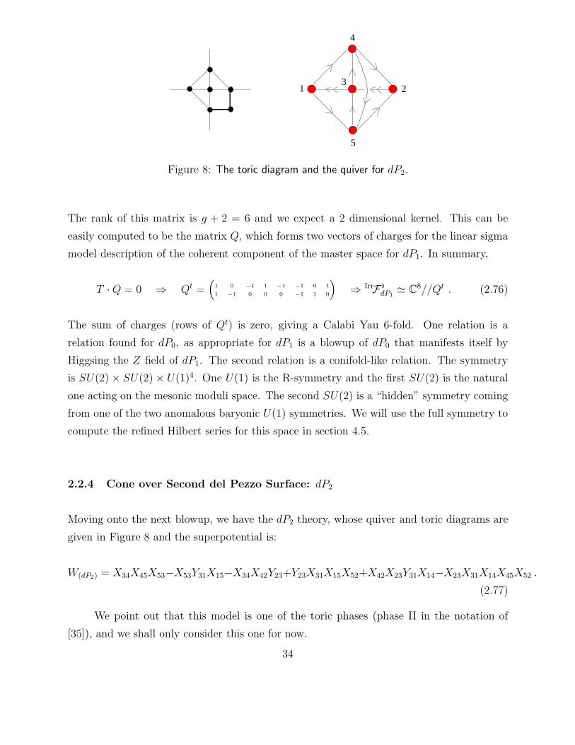
2.2.4 Cone over Second del Pezzo Surface: dP2

Moving onto the next blowup, we have the dP2 theory, whose quiver and toric diagrams are

given in Figure 8 and the superpotential is:

W(dP2) = X34X45X53−X53Y31X15−X34X42Y23+Y23X31X15X52+X42X23Y31X14−X23X31X14X45X52 .

(2.77)

We point out that this model is one of the toric phases (phase II in the notation of

[35]), and we shall only consider this one for now.

34

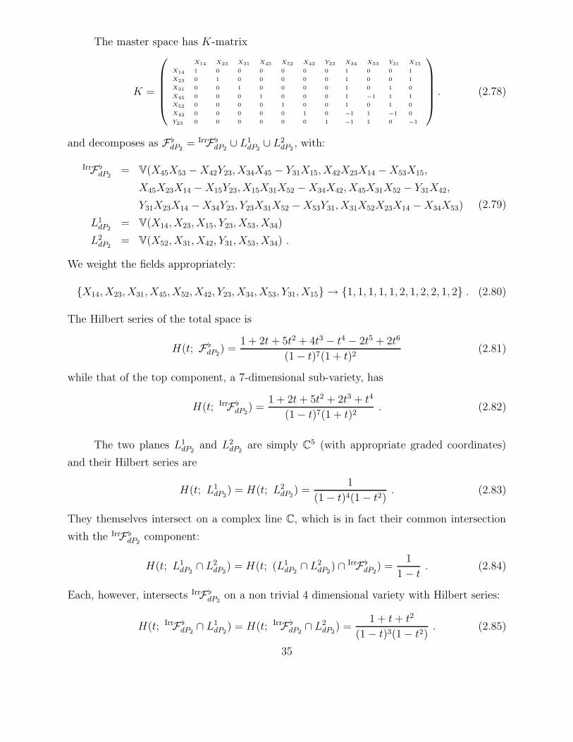
The master space has K-matrix

K =

X14 X23 X31 X45 X52 X42 Y23 X34 X53 Y31 X15

X14 1 0 0 0 0 0 0 1 0 0 1

X23 0 1 0 0 0 0 0 1 0 0 1

X31 0 0 1 0 0 0 0 1 0 1 0

X45 0 0 0 1 0 0 0 1 −1 1 1

X52 0 0 0 0 1 0 0 1 0 1 0

X42 0 0 0 0 0 1 0 −1 1 −1 0

Y23 0 0 0 0 0 0 1 −1 1 0 −1

. (2.78)

and decomposes as F ♭dP2

= IrrF ♭dP2

∪ L1dP2

∪ L2dP2

, with:

IrrF ♭dP2

= V(X45X53 − X42Y23, X34X45 − Y31X15, X42X23X14 − X53X15,

X45X23X14 − X15Y23, X15X31X52 − X34X42, X45X31X52 − Y31X42,

Y31X23X14 − X34Y23, Y23X31X52 − X53Y31, X31X52X23X14 − X34X53)

L1dP2

= V(X14, X23, X15, Y23, X53, X34)

L2dP2

= V(X52, X31, X42, Y31, X53, X34) .

(2.79)

We weight the fields appropriately:

{X14, X23, X31, X45, X52, X42, Y23, X34, X53, Y31, X15} → {1, 1, 1, 1, 1, 2, 1, 2, 2, 1, 2} . (2.80)

The Hilbert series of the total space is

H(t; F ♭dP2

) =1 + 2t + 5t2 + 4t3 − t4 − 2t5 + 2t6

(1 − t)7(1 + t)2(2.81)

while that of the top component, a 7-dimensional sub-variety, has

H(t; IrrF ♭dP2

) =1 + 2t + 5t2 + 2t3 + t4

(1 − t)7(1 + t)2. (2.82)

The two planes L1dP2

and L2dP2

are simply C5 (with appropriate graded coordinates)

and their Hilbert series are

H(t; L1dP2

) = H(t; L2dP2

) =1

(1 − t)4(1 − t2). (2.83)

They themselves intersect on a complex line C, which is in fact their common intersection

with the IrrF ♭dP2

component:

H(t; L1dP2

∩ L2dP2

) = H(t; (L1dP2

∩ L2dP2

) ∩ IrrF ♭dP2

) =1

1 − t. (2.84)

Each, however, intersects IrrF ♭dP2

on a non trivial 4 dimensional variety with Hilbert series:

H(t; IrrF ♭dP2

∩ L1dP2


∩ L2dP2

) =1 + t + t2

(1 − t)3(1 − t2). (2.85)

35

This is a manifold of complete intersection generated by 4 generators of degree 1 and

1 generator of degree 2 satisfying 1 relation of degree 3. Again, we have a surgery relation

among the Hilbert series, fully exhibiting the intersection structure of the components of the

master space:

H(t; F ♭dP2


) + H(t; L1dP2

) + H(t; L2dP2

) + H(t; (L1dP2

∩ L2dP2

) ∩ IrrF ♭dP2

)

−H(t; IrrF ♭dP2

∩ L1dP2

) − H(t; IrrF ♭dP2

∩ L2dP2

) − H(t; L1dP2

∩ L2dP2

) .

(2.86)

For reference, the dual cone T -matrix and the perfect matching matrix P = Kt ·T are:

T =

0 0 0 0 0 0 0 0 1 1

0 0 0 0 0 0 1 1 0 0

0 0 0 0 1 1 0 0 0 0

0 0 1 1 0 0 0 0 0 0

1 1 0 0 0 0 0 0 0 0

0 1 0 1 0 1 0 0 0 0

0 0 1 0 0 0 0 1 0 1

, P =

0 0 0 0 0 0 0 0 1 1

0 0 0 0 0 0 1 1 0 0

0 0 0 0 1 1 0 0 0 0

0 0 1 1 0 0 0 0 0 0

1 1 0 0 0 0 0 0 0 0

0 1 0 1 0 1 0 0 0 0

0 0 1 0 0 0 0 1 0 1

1 0 0 0 1 0 1 0 1 0

0 1 0 0 0 1 0 1 0 1

1 0 1 0 1 0 0 0 0 0

0 0 0 1 0 0 1 0 1 0

. (2.87)


Qt =

(1 −1 −1 1 0 0 0 0 −1 1

1 −1 −1 1 0 0 −1 1 0 0

1 −1 0 0 −1 1 0 0 0 0

)

⇒ IrrF ♭dP2

≃ C10//Qt . (2.88)

Once again, the rows of Qt sum to 0 and the toric variety is Calabi-Yau.

2.2.5 Cone over Third del Pezzo Surface: dP3

Now for the last true toric del Pezzo, let us study dP3, whose toric and quiver diagrams are

given in Figure 9 and superpotential:

W(dP3) = X12X23X34X45X56X61 + X13X35X51 + X24X46X62

−X23X35X56X62 − X13X34X46X61 − X12X24X45X51 . (2.89)

Again, we need to weight the variables appropriately:

{X12, X23, X34, X45, X56, X61, X13, X35, X51, X24, X46, X62} → {1, 1, 1, 1, 1, 1, 2, 2, 2, 2, 2, 2} .

(2.90)

Again, this is only one of the 4 toric phases of the theory (Phase I in the notation of [35]).

For now, we shall focus on this one.

36

6

1

2

3 5

4


The K-matrix for the master space is

K =

X12 X23 X45 X56 X46 X34 X61 X51 X13 X24 X62 X35

X12 1 0 0 0 0 0 0 0 1 −1 1 1

X23 0 1 0 0 0 0 0 0 1 0 1 0

X45 0 0 1 0 0 0 0 0 1 0 0 1

X56 0 0 0 1 0 0 0 0 1 −1 1 1

X46 0 0 0 0 1 0 0 0 1 0 1 0

X34 0 0 0 0 0 1 0 0 1 0 0 1

X61 0 0 0 0 0 0 1 0 −1 1 −1 0

X51 0 0 0 0 0 0 0 1 −1 1 0 −1

(2.91)

and F ♭dP3

decomposes as IrrF ♭dP3

∪ L1dP3

∪ L2dP3

∪ L3dP3

with

IrrF ♭dP3

= V(X23X56X62 − X13X51, X34X61X46 − X35X51, X12X45X24 − X13X35,

X12X45X51 − X46X62, X23X56X35 − X24X46, X34X61X13 − X24X62,

X23X34X56X61 − X51X24, X12X34X45X61 − X35X62, X12X23X45X56 − X13X46),

L1dP3

= V(X62, X46, X35, X13, X45, X12),

L2dP3

= V(X46, X24, X51, X13, X56, X23),

L3dP3

= V(X62, X24, X51, X35, X61, X34) .

(2.92)

We see that there are four irreducible sub-varieties: the 8 dimensional Calabi-Yau cone and

three 6 dimensional planes. The various Hilbert series are:

H(t; F ♭dP3

) = 1+4t2+4t4−6t5+3t6

(1−t)8(1+t)2; H(t; IrrF ♭

dP3) = 1+4t2+t4

(1−t)8(1+t)2,

H(t; L1dP3

) = H(t; L2dP3

) = H(t; L3dP3

) = 1(1−t)4(1−t2)2

.(2.93)

The planes L1dP3

, L2dP3

and L3dP3

intersect the IrrF ♭dP3

in a non-trivial 5-dimensional

variety with Hilbert series

H(t; IrrF ♭dP3

∩ L1dP3


∩ L2dP3


∩ L3dP3

) =1 + t2

(1 − t)4(1 − t2)(2.94)

37

and they intersect themselves in a complex plane C2, which is also their common intersection

with IrrF ♭dP3

; this intersection has Hilbert series

H(t; L1dP3

∩ L2dP3

) = H(t; L1dP3

∩ L3dP3

) = H(t; L2dP3

∩ L3dP3

) =

H(t; IrrF ♭dP3

∩ L1dP3

∩ L2dP3


∩ L1dP3

∩ L3dP3


∩ L2dP3

∩ L3dP3

) = 1(1−t)2

.

(2.95)

The common intersection among the three planes and among all the four irreducible

components of F ♭dP3

is just the origin of the embedding space. Once more, we have the

surgery relation

H(t; F ♭dP3


) + H(t; L1dP3

) + H(t; L2dP3

) + H(t; L3dP3


∩ L1dP3

)

− H(t; IrrF ♭dP3

∩ L2dP3


∩ L3dP3

) − H(t; L1dP3

∩ L2dP3

)

− H(t; L1dP3

∩ L3dP3

) − H(t; L2dP3

∩ L3dP3

) + H(t; IrrF ♭dP3

∩ L1dP3

∩ L2dP3

)+

H(t; IrrF ♭dP3

∩ L1dP3

∩ L3dP3

) + H(t; IrrF ♭dP3

∩ L2dP3

∩ L3dP3

) .

Finally, the dual cone T -matrix and the perfect matching matrix P = Kt · T are:

T =

0 0 0 0 0 0 0 0 0 0 1 1

0 0 0 0 0 0 0 0 1 1 0 0

0 0 0 0 0 0 1 1 0 0 0 0

0 0 0 0 1 1 0 0 0 0 0 0

0 0 1 1 0 0 0 0 0 0 0 0

1 1 0 0 0 0 0 0 0 0 0 0

0 0 0 1 0 1 0 0 0 1 0 1

0 1 0 0 1 0 0 1 0 0 1 0

, P =

0 0 0 0 0 0 0 0 0 0 1 1

0 0 0 0 0 0 0 0 1 1 0 0

0 0 0 0 0 0 1 1 0 0 0 0

0 0 0 0 1 1 0 0 0 0 0 0

0 0 1 1 0 0 0 0 0 0 0 0

1 1 0 0 0 0 0 0 0 0 0 0

0 0 0 1 0 1 0 0 0 1 0 1

0 1 0 0 1 0 0 1 0 0 1 0

1 0 1 0 0 0 1 0 1 0 0 0

0 1 0 1 0 0 0 1 0 1 0 0

0 0 1 0 1 0 0 0 1 0 1 0

1 0 0 0 0 1 1 0 0 0 0 1

.

(2.96)


Qt =

(−1 1 1 −1 0 0 0 0 0 0 −1 1

0 0 1 −1 0 0 0 0 −1 1 0 0

1 −1 0 0 0 0 −1 1 0 0 0 0

−1 1 1 −1 −1 1 0 0 0 0 0 0

)

⇒ IrrF ♭dP3

≃ C12//Qt . (2.97)

We see that the rows of Qt sum to 0 and the toric variety is Calabi-Yau.

2.2.6 Cone over Fourth Pseudo del Pezzo Surface: PdP4

By blowing dP3 up at a non-generic point we can obtain another toric variety, referred to

as a pseudo del Pezzo [34]. The toric and quiver diagrams are given in Figure 10 and the

superpotential is

WPdP4 = X61X17X74X46 + X21X13X35X52 + X27X73X36X62 + X14X45X51

−X51X17X73X35 − X21X14X46X62 − X27X74X45X52 − X13X36X61 .

38

7

1

2

6

5 4

3

Figure 10: The toric diagram and the quiver for PdP4.

Once again, we need to assign appropriate weights to the variables:

{X45, X73, X46, X21, X36, X74, X52, X35, X17, X62, X51, X27, X61, X13, X14}→ {2, 2, 2, 2, 2, 2, 2, 2, 2, 2, 4, 4, 4, 4, 4} .

(2.98)

Subsequently, the K-matrix is given as

K =

X13 X17 X35 X61 X14 X27 X62 X51 X74 X45 X36 X46 X21 X73 X52

X13 1 0 0 0 0 0 0 0 0 1 0 1 0 1 0

X17 0 1 0 0 0 0 0 0 0 1 1 0 1 0 0

X35 0 0 1 0 0 0 0 0 0 1 1 1 0 0 0

X61 0 0 0 1 0 0 0 0 0 1 0 0 1 1 0

X14 0 0 0 0 1 0 0 0 0 −1 0 0 −1 0 1

X27 0 0 0 0 0 1 0 0 0 −1 −1 −1 0 −1 −1

X62 0 0 0 0 0 0 1 0 0 −1 −1 −1 −1 −1 0

X51 0 0 0 0 0 0 0 1 0 0 1 1 0 0 1

X74 0 0 0 0 0 0 0 0 1 0 0 −1 1 0 −1

. (2.99)

and the master space has Hilbert series

H(t; F♭PdP4

) =1 − 5t6 − 10t8 + 8t10 + 26t12 + 67t14 − 162t16 − 56t18 + 276t20 − 111t22 − 122t24 + 112t26 − 14t28 − 15t30 + 5t32

(1 − t4)5(1 − t2)10.

(2.100)

Now, F ♭PdP4

has a top IrrF ♭PdP4

component of dimension 9:

IrrF♭PdP4

= V(X46X21X62 − X45X51, X73X35X17 − X45X14, X46X74X17 − X36X13, X21X52X35 − X36X61,

X45X74X52 − X73X36X62, X52X35X13 − X46X62X14, X74X17X61 − X21X62X14, X73X62X27 − X61X13,

X74X52X27 − X51X14, X45X52X27 − X46X17X61, X45X74X27 − X21X35X13, X73X36X27 − X46X21X14,

X35X17X51 − X36X62X27, X73X17X51 − X21X52X13, X73X35X51 − X46X74X61, X73X46X17X62 − X45X52X13,

X73X21X35X62 − X45X74X61, X74X52X35X17 − X36X62X14, X46X21X35X17 − X45X36X27, X46X21X74X52 − X73X36X51,

X21X52X62X27 − X17X51X61, X46X74X62X27 − X35X51X13, X73X74X17X27 − X21X13X14, X73X52X35X27 − X46X61X14) ,

(2.101)

with Hilbert series

H(t; IrrF ♭PdP4

) =1 + t2 + 6t4 + t6 + t8

(1 − t2)9. (2.102)

39

The dual cone T -matrix and the perfect matching matrix P = Kt · T are:

T =

0 0 0 0 0 0 0 0 0 0 0 0 1 1 1 1 1 1

0 0 0 0 0 0 0 0 0 0 1 1 0 0 0 0 1 1

0 0 0 0 0 0 1 1 1 1 0 0 0 0 0 0 0 0

0 0 1 1 1 1 0 0 1 1 0 0 0 0 0 0 0 0

0 0 0 0 0 1 0 1 0 1 0 1 0 0 0 1 0 1

0 0 0 0 1 0 0 0 0 1 0 0 0 0 1 0 0 1

0 0 0 1 0 0 0 0 1 0 0 0 0 1 0 0 1 0

1 1 0 1 1 0 0 0 0 0 0 0 0 1 1 0 0 0

0 1 0 0 0 0 0 1 0 0 0 0 0 1 0 1 0 0

,

P =

0 0 0 0 0 0 0 0 0 0 0 0 1 1 1 1 1 1

0 0 0 0 0 0 0 0 0 0 1 1 0 0 0 0 1 1

0 0 0 0 0 0 1 1 1 1 0 0 0 0 0 0 0 0

0 0 1 1 1 1 0 0 1 1 0 0 0 0 0 0 0 0

0 0 0 0 0 1 0 1 0 1 0 1 0 0 0 1 0 1

0 0 0 0 1 0 0 0 0 1 0 0 0 0 1 0 0 1

0 0 0 1 0 0 0 0 1 0 0 0 0 1 0 0 1 0

1 1 0 1 1 0 0 0 0 0 0 0 0 1 1 0 0 0

0 1 0 0 0 0 0 1 0 0 0 0 0 1 0 1 0 0

0 0 1 0 0 0 1 0 1 0 1 0 1 0 0 0 1 0

1 1 0 0 0 0 1 1 0 0 1 1 0 0 0 0 0 0

1 0 0 0 0 0 1 0 0 0 0 0 1 0 1 0 0 0

0 1 1 0 1 0 0 0 0 0 1 0 0 0 0 0 0 0

0 0 1 0 0 1 0 0 0 0 0 0 1 0 0 1 0 0

1 0 0 1 0 1 0 0 0 0 0 1 0 0 0 0 0 0

.

(2.103)


Qt =

0 0 1 1 −1 −1 0 0 0 0 0 0 0 0 0 0 −1 1

1 0 1 −1 0 0 0 0 0 0 −1 0 −1 0 0 0 1 0

1 −1 1 0 0 −1 0 0 0 0 0 0 −1 0 0 1 0 0

0 0 1 0 −1 0 0 0 0 0 0 0 −1 0 1 0 0 0

1 −1 1 −1 0 0 0 0 0 0 0 0 −1 1 0 0 0 0

0 0 1 0 0 −1 0 0 0 0 −1 1 0 0 0 0 0 0

1 0 1 0 −1 −1 −1 0 0 1 0 0 0 0 0 0 0 0

1 0 0 −1 0 0 −1 0 1 0 0 0 0 0 0 0 0 0

1 −1 1 0 0 −1 −1 1 0 0 0 0 0 0 0 0 0 0

⇒ IrrF ♭PdP4

≃ C18//Qt .

(2.104)

Indeed, the rows of Qt sum to 0 and the toric variety is Calabi-Yau.

2.2.7 Cone over Fifth Pseudo del Pezzo Surface: PdP5

Trudging on, we can also study one more blowup, the PdP5 theory. The toric and quiver

diagrams are given in Figure 11 and the superpotential is

WPdP5 = −X13X35X58X81 + X14X46X68X81 + X35X57X72X23 − X46X67X72X24

+X67X71X13X36 − X57X71X14X45 + X58X82X24X45 − X68X82X23X36 .

(2.105)

Now, all the variables have the same weight and the master space has K-matrix

40

3

1

2 7

4

6

8 5

Figure 11: The toric diagram and the quiver for PdP5.

K =

X24 X36 X67 X82 X35 X57 X81 X45 X46 X68 X14 X13 X23 X72 X58 X71

X24 1 0 0 0 0 0 0 0 0 0 1 1 1 0 0 0

X36 0 1 0 0 0 0 0 0 0 0 1 0 0 1 1 0

X67 0 0 1 0 0 0 0 0 0 0 1 0 1 0 1 0

X82 0 0 0 1 0 0 0 0 0 0 1 1 0 1 0 0

X35 0 0 0 0 1 0 0 0 0 0 −1 −1 −1 −1 −1 0

X57 0 0 0 0 0 1 0 0 0 0 −1 0 −1 −1 −1 −1

X81 0 0 0 0 0 0 1 0 0 0 −1 −1 0 0 0 1

X45 0 0 0 0 0 0 0 1 0 0 0 1 0 0 −1 −1

X46 0 0 0 0 0 0 0 0 1 0 0 0 1 0 1 1

X68 0 0 0 0 0 0 0 0 0 1 0 0 0 1 1 1

,

(2.106)

as well as the Hilbert series

H(t; F ♭PdP5

) =1 + 6t + 21t2 + 40t3 + 39t4 − 30t5 + 19t6

(−1 + t)10. (2.107)

The top component is Calabi-Yau of dimension 10 given by the intersection:

IrrF♭PdP5

= V(X13X67X36 − X14X57X45, X68X23X36 − X58X24X45, X13X67X71 − X68X23X82, X14X57X71 − X58X24X82,

X46X72X24 − X13X71X36, X46X72X67 − X58X45X82, X35X72X23 − X14X71X45, X35X57X23 − X46X67X24,

X35X57X72 − X68X36X82, X81X46X68 − X57X71X45X81X14X68 − X72X67X24, X81X14X46 − X23X36X82,

X35X58X81 − X67X71X36, X13X58X81 − X57X72X23, X13X35X81 − X24X45X82, X13X35X58 − X14X46X68,

X72X23X67X36 − X58X81X14X45, X46X68X67X36 − X35X58X57X45, X13X35X23X36 − X14X46X24X45,





X14X46X57X72 − X13X58X36X82, X35X81X46X72 − X71X36X45X82, X35X81X14X57 − X67X24X36X82)

(2.108)

and has Hilbert series

H(t; IrrF ♭PdP5

) =1 + 6t + 21t2 + 40t3 + 21t4 + 6t5 + t6

(1 − t)10. (2.109)

41

Finally, the dual cone T -matrix and the perfect matching matrix P = Kt · T are:

T =

0 0 0 0 0 0 0 0 0 0 0 0 0 0 0 0 0 0 1 1 1 1 1 1

0 0 0 0 0 0 0 0 0 0 0 0 0 0 1 1 1 1 0 0 0 0 1 1

0 0 0 0 0 0 0 0 1 1 1 1 1 1 0 0 0 0 0 0 0 0 0 0

0 0 0 0 1 1 1 1 0 0 0 0 1 1 0 0 0 0 0 0 0 0 0 0

0 0 0 0 0 0 0 1 0 0 0 1 0 1 0 0 0 1 0 0 0 1 0 1

0 0 0 0 0 0 1 0 0 0 1 0 1 0 0 0 1 0 0 0 1 0 1 0

0 0 0 0 0 1 0 0 0 1 0 0 1 0 0 1 0 0 0 1 0 0 1 0

0 0 1 1 0 0 0 0 0 1 0 1 0 0 0 1 0 1 0 0 0 0 0 0

0 1 0 1 0 0 1 1 0 0 0 0 0 0 0 0 1 1 0 0 0 0 0 0

1 0 1 0 0 0 0 0 0 0 1 1 0 0 0 0 0 0 0 0 1 1 0 0

,

P =

0 0 0 0 0 0 0 0 0 0 0 0 0 0 0 0 0 0 1 1 1 1 1 1

0 0 0 0 0 0 0 0 0 0 0 0 0 0 1 1 1 1 0 0 0 0 1 1

0 0 0 0 0 0 0 0 1 1 1 1 1 1 0 0 0 0 0 0 0 0 0 0

0 0 0 0 1 1 1 1 0 0 0 0 1 1 0 0 0 0 0 0 0 0 0 0

0 0 0 0 0 0 0 1 0 0 0 1 0 1 0 0 0 1 0 0 0 1 0 1

0 0 0 0 0 0 1 0 0 0 1 0 1 0 0 0 1 0 0 0 1 0 1 0

0 0 0 0 0 1 0 0 0 1 0 0 1 0 0 1 0 0 0 1 0 0 1 0

0 0 1 1 0 0 0 0 0 1 0 1 0 0 0 1 0 1 0 0 0 0 0 0

0 1 0 1 0 0 1 1 0 0 0 0 0 0 0 0 1 1 0 0 0 0 0 0

1 0 1 0 0 0 0 0 0 0 1 1 0 0 0 0 0 0 0 0 1 1 0 0

0 0 0 0 1 0 0 0 1 0 0 0 0 1 1 0 0 0 1 0 0 0 0 1

0 0 1 1 1 0 1 0 0 0 0 0 0 0 0 0 0 0 1 0 1 0 0 0

0 1 0 1 0 0 0 0 1 1 0 0 0 0 0 0 0 0 1 1 0 0 0 0

1 0 1 0 1 1 0 0 0 0 0 0 0 0 1 1 0 0 0 0 0 0 0 0

1 1 0 0 0 0 0 0 1 0 1 0 0 0 1 0 1 0 0 0 0 0 0 0

1 1 0 0 0 1 0 1 0 0 0 0 0 0 0 0 0 0 0 1 0 1 0 0

.

(2.110)


Qt =

0 1 0 0 1 0 0 −1 0 0 0 0 0 0 −1 0 0 0 −1 0 0 0 0 1

0 0 0 0 1 −1 −1 1 0 0 0 0 0 0 0 0 0 0 0 0 0 0 1 −1

−1 1 0 0 1 0 0 −1 0 0 0 0 0 0 0 0 0 0 −1 0 0 1 0 0

−1 1 0 0 1 0 −1 0 0 0 0 0 0 0 0 0 0 0 −1 0 1 0 0 0

0 0 0 0 1 −1 0 0 0 0 0 0 0 0 0 0 0 0 −1 1 0 0 0 0

1 0 −1 0 1 0 0 −1 0 0 0 0 0 0 −1 0 0 1 0 0 0 0 0 0

0 0 0 0 1 0 −1 0 0 0 0 0 0 0 −1 0 1 0 0 0 0 0 0 0

1 0 −1 0 1 −1 0 0 0 0 0 0 0 0 −1 1 0 0 0 0 0 0 0 0

0 1 0 0 0 0 0 −1 −1 0 0 0 0 1 0 0 0 0 0 0 0 0 0 0

0 1 0 0 1 −1 −1 0 −1 0 0 0 1 0 0 0 0 0 0 0 0 0 0 0

0 1 −1 0 1 0 0 −1 −1 0 0 1 0 0 0 0 0 0 0 0 0 0 0 0

−1 1 0 0 1 0 −1 0 −1 0 1 0 0 0 0 0 0 0 0 0 0 0 0 0

1 0 −1 0 1 −1 0 0 −1 1 0 0 0 0 0 0 0 0 0 0 0 0 0 0

1 −1 −1 1 0 0 0 0 0 0 0 0 0 0 0 0 0 0 0 0 0 0 0 0

⇒ IrrF ♭PdP5

≃ C24//Qt .

(2.111)

Again, the rows of Qt sum to 0 and the toric variety is Calabi-Yau.

2.3 The Master Space: Recapitulation

Having warmed up with an etude and some developmental case studies let us recapitulate

with our theme in F ♭. We have studied, with extensive examples for toric theories at number

of D3-branes equaling to N = 1, the algebraic variety formed by the F-flatness equations,

we have seen that in general this is a reducible variety, with a top Calabi-Yau component

42

of dimension g + 2. In this section we recapitulate and deepen the properties of the master

space F ♭ for such toric quiver gauge theories and will discuss what happens for N > 1.

2.3.1 The Toric N = 1 Case

As we have seen, F ♭ is a toric g + 2 dimensional variety, not necessarily irreducible. The

coherent component IrrF ♭, the largest irreducible component of F ♭, also of dimension g + 2,

can be quite explicitly characterized. Denoting, as usual, with E the number of fields in the

quiver, g the number of nodes in the quiver and with c the number of perfect matchings in

the dimer realization of the gauge theory, we have defined three matrices:

• A (g+2)×E matrix K obtained by solving the F-terms in terms of a set of independent

fields. The columns give the charges of the elementary fields under the (C∗)g+2 action;

in a more mathematical language, they give the semi-group generators of the cone σ∨K

in the toric presentation for IrrF ♭:

IrrF ♭ ≃ SpecC[σ∨K ∩ Z

g+2] (2.112)

• A (g + 2) × c matrix T , defined by Kt · T ≥ 0, and representing the dual cone σK .

The columns are the c toric vectors of the g + 2 dimensional variety IrrF ♭. We see that

the number of perfect matchings in the dimer realization of the quiver theory is the

number of external points in the toric diagram for IrrF ♭. This generalizes the fact that

the external perfect matchings are related to the external points of the toric diagram

for the three dimensional transverse Calabi-Yau space X .

• A E × c matrix P = Kt · T which defines the perfect matchings as collections of

elementary fields.

The variety IrrF ♭ also has a linear sigma model, or symplectic quotient, description as

IrrF ♭ = Cc//Qt , (2.113)

where Q is the kernel of the matrices P and T . From all these descriptions we can extract

some general properties of the master space and of its Hilbert series.

43

As a Higher-Dimensional Calabi-Yau: The most suggestive property is that IrrF ♭ is

always a g + 2 dimensional Calabi-Yau manifold. This has been explicitly checked in all the

examples we have discussed. It is simple to check the Calabi-Yau condition in the linear

sigma model description, since it corresponds there to the fact that the vectors of charges

in Qt are traceless, or equivalently, the toric diagram has all the vectors ending on the same

hyper-plane.

There is a remarkably simple proof that IrrF ♭ is Calabi-Yau which emphasizes the role of

perfect matchings. Recall from [6] and §2.1.7 that the quiver gauge theory has a description

in terms of a dimer model, this is a bi-partite tiling of the two torus, with V/2 white vertices

and V/2 black vertices, where V is the number of superpotential terms. The elementary

fields of the quiver correspond to the edges in the tiling, each of which connects a black

vertex to a white one. Now, by definition, a perfect matching is a choice of fields/dimers

that cover each vertex precisely once. In particular, a perfect matching contains exactly V/2

dimers, connecting the V/2 black vertices to the V/2 white ones. Since the columns of the

matrix P , of size E × c, tell us which fields/dimers occur in a given perfect matching we

have the nice identity

(1, 1, ...., 1)︸︷︷︸

E

·P =V

2(1, 1, ...., 1)︸︷︷︸

c

, (2.114)

which basically counts the number of edges in each perfect matching.

By multiplying this equation on the right by the matrix kernel Q of P , P · Q = 0, we

obtain

0 = (1, 1, ...., 1)︸︷︷︸

c

·Q (2.115)

and we conclude that the vector of charges of the linear sigma model, which are the rows of

the matrix Qt, are traceless. This proves that IrrF ♭ is Calabi-Yau.

We again see that the prefect matchings description is crucial in our understanding of

the properties of the master space. As explained in §2.1.7, the perfect matchings generates

the coherent component of the master space as a consequence of the Birkhoff-Von Neumann

Theorem.

Seiberg Duality: From our study of the toric dual phases, exemplified above by the two

phases of the cone over the Hirzebruch surface, we conjecture that

44

For a pair of Seiberg dual theories, IrrF ♭ is the same for both.

Palindromic Hilbert Series: An intriguing property of the Hilbert series for IrrF ♭ is its

symmetry. As manifest from all our examples, the numerator of the Hilbert series (in second

form) for IrrF ♭ is a polynomial in t

P (t) =

N∑

k=0

aktk (2.116)

with symmetric coefficients aN−k = ak. This means that there is a remarkable symmetry of

the Hilbert series for IrrF ♭ under t → 1/t,

H(1/t; IrrF ♭) = twH(t; IrrF ♭) (2.117)

where the modular weight w depends on IrrF ♭.

A polynomial with such a symmetry between its consecutively highest and lowest co-

efficients aN−k ↔ ak is known as a palindromic polynomial. A beautiful theorem due to

Stanley [36] states the following

THEOREM 2.1 The numerator to the Hilbert series of a graded Cohen-Macaulay domain

R is palindromic iff R is Gorenstein.

What this means, for us, is that the coordinate ring of the affine variety IrrF ♭ must be

Gorenstein. However, an affine toric variety is Gorenstein precisely if its toric diagram is

co-planar, i.e., it is Calabi-Yau (cf. e.g. § 4.2 of [30]). Thus we have killed two birds with one

stone: proving that IrrF ♭ is affine toric Calabi-Yau above from perfect matchings also shows

that the numerator of its Hilbert series has the palindromic symmetry.

As we will see, this symmetry extends to the refined Hilbert series written in terms

of the R-charge parameter t and chemical potentials for a global symmetry G. Although

G has been up to now Abelian, we will see that in some special cases of theories with

hidden symmetries G becomes non Abelian. Introducing chemical potentials z for Cartan

sub-algebra of G, we will write the refined Hilbert series as a sum over G-characters in the

general form,

H(t, G) =

(N∑

k=0

χk(z)tk

)

PE

[G∑

i=1

χi(z)ti

]

(2.118)

45

where PE is the plethystic exponential to be reviewed in §2.3.3, computing symmetric prod-

ucts on a set of generators of the coherent component. The refined Hilbert series is now

invariant under the the combined action of t → 1/t and charge conjugation, χN−k = χ∗k. We

will see many examples in Section 4.

2.3.2 General N

The case for an arbitrary number N of D3-branes is much more subtle and less understood in

the mathematical literature 5, even though it is clear from the gauge theory perspective. We

know that the world-volume theory for N D3-branes is a quiver theory with product U(Ni)

gauge groups and in the IR, the U(1) factors decouple since only the special unitary groups

exhibit asymptotic freedom and are strongly coupled in the IR. Thus the moduli space of

interest is the space of solutions to the F-flatness, quotiented out by a non-Abelian gauge

group

MN = F ♭N/(SU(N1) × . . . × SU(Ng)). (2.119)

where the index N recalls that we are dealing with N branes. The moduli space MN is of

difficult characterization since the quotient is fully non-Abelian and it can not be described

by toric methods, as in the N = 1 case.

The more familiar mesonic moduli space is obtained by performing a further quotient

by the Abelian symmetries. Even for N branes, the Abelian group will be constituted of

the decoupled U(1) factors, and hence will be the same as in the toric, N = 1 case. Once

again, we expect to have some symplectic quotient structure, in analogy with (1.2), for this

mesonic moduli space:

mesMN ≃ MN//U(1)g−1 . (2.120)

Hence, a toric symplectic quotient still persists for (2.120), even though the moduli space in

question is not necessarily toric.

Moreover, our plethystic techniques, which we will shortly review, will illuminate us

with much physical intuition. First, the mesonic moduli space for N branes is the N -th

symmetrized product of that of N = 1:

mesMN ≃ SymNX := XN/ΣN , (2.121)

5We thank Balazs Szendroi for discussions on this point.

46

where ΣN is the symmetric group on N elements. We see that the mesonic moduli space,

for X a Calabi-Yau threefold, is of dimension 3N by (2.121). The dimension of the moduli

space MN is thus 3N + g − 1 for general N .

2.3.3 The Plethystic Programme Reviewed

We cannot embark upon a study of general N without delving into the plethystic programme,

whose one key purpose of design was for this treatment. Here let us review some essentials,

partly to set the notation for some extensive usage in §4 later. The realisation in [9] is that

the mesonic generating function, with all baryonic numbers fixed to be zero, g1,0(t; X ) =

f∞(t; X ) for the single-trace mesonic operators for D3-branes probing a Calabi-Yau threefold

X at N → ∞ is the Hilbert series of X . Let us define the Plethystic Exponential of a

multi-variable function g(t1, . . . , tn) that vanishes at the origin, g(0, . . . , 0) = 0, to be

PE [g(t1, . . . , tn)] := exp

(∞∑

k=1

g(tk1, . . . , tkn)

k

)

. (2.122)

Then the multi-trace mesonic operators at N → ∞ are counted by the plethystic

exponential6

g∞,0(t; X ) = PE[f∞(t; X ) − 1] := exp

(∞∑

r=1

f∞(tr) − 1

r

)

. (2.123)

The inverse, f1(t; X ) = PE−1[f∞(t; X )], is counting objects in the defining equation

(syzygy) of the threefold. The mesonic multi-trace generating function gN at finite N is

found by the series expansion of the ν-inserted plethystic exponential7 as

PE[νf∞(t; X )] = exp

(∞∑

r=1

νrf∞(tr)

r

)

=∞∑

N=0

gN(t)νN . (2.124)

In general [11], for the combined mesonic and baryonic branches of the moduli space8,

the N = 1 operators are counted by the Hilbert series of the master space. The plethystic

6Note that in order to avoid an infinity the PE is defined with respect to a function that vanishes when

all chemical potentials are set to zero.7Note that the ν insertion satisfies the condition that the argument of PE vanishes when all chemical

potentials are set to zero. Any attempt to subtract something from this function leads to incorrect results.8To be Strict, we should say here the mesonic branch together with given FI-parameters, since at N = 1,

47

program can be efficiently applied to the study of the coherent component of the moduli

space [12]. With the generating function for the coherent component of the master space,

which we denote g1(t; X ) ≡ H(t; IrrF ♭), we can proceed with the plethystic program and

find the result for gN(t; X ), counting the combined baryonic and mesonic gauge invariant

operators at finite N .

The implementation of the plethystic program requires a decomposition of the g1(t; X )

generating function in sectors of definite baryonic charge, to which the plethystic exponential

is applied. An interesting connection of this decomposition is found in [12, 11] with Kahler

moduli. This also enables a different computation of g1(t; X ). Though our current techniques

compute this quantity using the Hilbert series of the master space, we will later check that

this indeed agrees with the formalism of [12].

The decomposition of g1(t; X ) requires the knowledge of two sets of partition functions,

the geometrical ones, obtained by localization, and the auxiliary one, obtained from dimer

combinatorics. Specifically, it was realized that

g1(t; X ) =∑

P∈GKZ

m(P )g1,P (t; X ) (2.125)

where the summation is extended over the lattice points P , of multiplicity m(P ), of a so-

called GKZ (or secondary) fan of the Calabi-Yau threefold and g1,P is a much more

manageable object obtained from a localisation computation, as given in Eq (4.18) of [12].

The GKZ fan, to remind the reader, is the fan of an auxiliary toric variety, which is the space

of Kahler parameters of the original toric threefold X . This space is of dimension I − 3 + d,

where I is the number of internal points and d, the number of vertices, of the toric diagram

of X .

The multiplicity m(P ) of points in this GKZ lattice fan is counted by an auxiliary

partition function, so-named Zaux. This is simply the (refined) Hilbert series of the follow-

ing space: take the simpler quiver than the original by neglecting any repeated arrows and

then form the space of open but not closed loops in this simplified quiver. The expansion of

Zaux can then be used to compute the generating function for one D3-brane.

As a brief reminder to the reader, the procedure to determine the refined generat-

ing function g1 in (2.125) is to (1) obtain the generating function g1,β1,...βKin terms of a

there are no baryons. Nevertheless, we can still generate the counting for the baryons for N > 1 using PE

of the N = 1 case.

48

set of Kahler parameters β1, ..., βK using the localisation formula (4.18) of [12]; (2) obtain

Zaux(t1, ..., tK) as above, and (3) replace a term tβ1

1 ...tβK

K in Zaux by an expression for g1,β1,...βK.

We will not enter in the details of this construction and we refer the reader to [12]. The

important point for our ensuing discussions is that the plethystic program can be applied to

the N = 1 partition functions at each point of the GKZ fan in order to obtain the finite N

generating function

g(t; X ) :=∞∑

N=0

νNgN(t; X ) =∑

P∈GKZ

m(P )PE [νg1,P (t; X )] . (2.126)

3 Linear Branches of Moduli Spaces

From the previous section we learned that the master space F ♭ of an N = 1 quiver gauge

theory on a toric singularity X generically presents a reducible moduli space. This fact

could appear surprising. Indeed the N = 2 supersymmetric gauge theories are the classical

examples of theories with reducible moduli spaces. These theories present two well separated

branches: the Higgs branch and the Coulomb branch. Moving along these different branches

has a well defined characterization both in terms of the geometry of the moduli space and

in terms of the VEV structure of the gauge theory. It would be interesting to have a similar

interpretation in this more generic setup9.

In the case of just N = 1 brane on the tip of the conical singularity X , the reducibility

of F ♭ follows easily from the toric condition. Indeed, the equations defining F ♭ are of the

form “monomial = monomial”, whereby giving us toric ideals as discussed in §2.1.4. Let us

embed this variety into Cd with coordinates {x1, ..., xd}, then its algebraic equations have

the form:

xij11 ...x

ijd

d

(

M1j(x) − M2j

(x))

= 0 , (3.1)

where j = 1, ..., k runs over the number of polynomials defining the variety and the poly-

nomials M1j(x) − M2j

(x) are irreducible. If some ijp is different from zero the variety is

reducible and is given by the union of the zero locus of M1j(x)−M2j

(x) together with a set

of planes (linear components) Ll given by the zero locus of the factorized part in (3.1).

9One can clearly look for other interpretations of the reducibility of F ♭. An interesting line of research

would be to connect the geometrical structure of F ♭ to the pattern of BPS branes in X . We will leave this

topic for future work.

49

(0,1,1)

(0,0,1) (1,0,1)21 (−1.0,1)

φ

1B

2B

1A

2A

2φ1

Figure 12: Quiver and toric diagrams for (C2/Z2) × C.

Hence, the master space F ♭ could be the union of a generically complicated g + 2

dimensional variety with a set of smaller dimensional linear varieties {Cd1 , ..., Cdn} param-

eterized by combinations of the coordinates10; this is certainly true for the extensive case

studies seen above in §2.2. It would be nice to give a gauge theory interpretation to these

smaller dimensional linear branches.

In the following subsections we will give a nice picture for these planes, for some selected

examples. The lesson we will learn is that these planes of the master space could parametrize

flows in the gauge theory. Specifically, there may be chains of flows from one irreducible

component of the master space of a theory to another. The archetypal example which will

be the terminus of many of these flows will be the gauge theory on a D3-brane probing the

Calabi-Yau singularity C2/Z2 × C, to which we alluded in §2.1.7. Let us first briefly review

this theory, continuing along the same vein as our discussions in §2.1.3.

3.1 The (C2/Z2) × C Singularity

The quiver gauge theory for (C2/Z2) × C has N = 2 supersymmetry with two vector mul-

tiplets and two bi-fundamental hyper-multiplets. In N = 1 notation we have six chiral

multiplets denoted as φ1, φ2, A1, A2, B1, B2, with a superpotential

W = φ1(A1B1 − A2B2) + φ2(B2A2 − B1A1) (3.2)

and the quiver and toric diagrams are given in Figure 12. The master space F ♭(C2/Z2)×C

of

10The reducibility of the moduli space could persist for N > 1, the simplest example being the conifold

with N = 2 (see [12] with other examples) and it would be interesting to have a clearer geometric picture

even in these more complicated cases. In this section we will concentrate on the N = 1 case.

50

the theory can be easily found to be

F ♭(C2/Z2)×C

= V(A1B1−A2B2, φ1A1 −φ2A1, φ1A2−φ2A2, φ1B1 −φ2B1, φ1B2−φ2B2) . (3.3)

Now, F ♭(C2/Z2)×C

is clearly reducible and decomposes into the following two irreducible com-

ponents as F ♭(C2/Z2)×C

= IrrF ♭(C2/Z2)×C

∪ L with

IrrF ♭(C2/Z2)×C

= V(φ1 − φ2, A1B1 − A2B2) , L = V(A1, A2, B1, B2) . (3.4)

Specifically, IrrF ♭(C2/Z2)×C

is C × C, where the C is defined by φ1 = φ2 and the conifold

singularity C is described by the chiral fields {A1, A2, B1, B2} with the constraint A1B1 =

A2B2. The component L = C2 is parametrized by the fields {φ1, φ2}. These two branches

meet on the complex line parametrized by φ1 = φ2.

The field theory interpretation of these two branches is standard: moving in L we are

giving VEV to the scalars in the vector multiplet and hence we call L the Coulomb branch;

while moving in IrrF ♭(C2/Z2)×C

we are giving VEV to the scalars in the hyper-multiplets and

hence we call IrrF ♭(C2/Z2)×C

the Higgs branch. Let us go on and revisit the reducibility of

some of the master spaces studied in the previous section trying to give them a gauge theory

interpretation.

3.2 Case Studies Re-examined

First Toric Phase of F0: Let us start by re-examining (F0)I , encountered in §2.2.2. We

recall from (2.49) that the master space F ♭F0

is the union of three branches: the biggest one

is six dimensional and is the set product of two conifold singularities, i.e., C ×C, and the two

smallest ones are two copies of C4, parametrized respectively by the VEV of {B1, B2, D1, D2}and {A1, A2, C1, C2}.

Looking at the toric diagram11 one can easily understand that the gauge theory can

flow to the one associated to the C2/Z2 × C singularity in four different ways by giving

11We remind the reader that the prescription is as follows [4, 5, 34]. If one toric diagram is derived

by deleting external vertices of the other, then the associated gauge theories can flow one into the other.

Geometrically this is blowing up the singularity, while in the gauge theory a FI term is turned on and as a

consequence gives VEV to some chiral fields, for a product of U(Ni) gauge groups; or a baryonic VEV is

turned on in the case of product of SU(Ni) gauge groups. It is indeed possible to associate fields of the gauge

theory to each vertex in the toric diagram, as shown in Figure 13. The deleted vertex can be associated with

the fields that are getting a VEV.

51

,1 C 1

A 2 C2

B1 D1

2DB2

,

,

,

A

Figure 13: The four possible flows from F0 to (C2/Z2) × C as exhibited in the toric diagrams.

VEV to one out of the four possible sets of fields: {A1, C1}, {A2, C2}, {B1, D1}, {B2, D2}.Once arrived at the fixed point one can move along the Coulomb branch of the IR theory

giving VEV respectively to the set of fields: {A2, C2}, {A1, C1}, {B2, D2}, {B1, D1}. Hence,

along the two smaller branches of the moduli space the theory admits an accidental N = 2

supersymmetry and the theory moves along the Coulomb branch of the resulting gauge

theory.

First del Pezzo: In (2.69) we saw that F ♭dP1

decomposes into two irreducible parts:IrrF ♭

dP1and L. The former is a six dimensional variety, while the existence of the latter four

dimensional linear variety L parametrized by {U1, U2, U1, U2} can be interpreted as the effect

of the presence of an accidental N = 2 sector.

Indeed, looking at the toric diagram (see figure 7) it is easy to realize that the theory

flows to the N = 2 theory of (C2/Z2) × C in two different ways: giving VEV to {U1, U1} or

to {U2, U2}, and the Coulomb branch of these ones is parametrized respectively by {U2, U2}and {U1, U1}. Hence, as in the case of F0 the linear component in the reducible master space

parameterizes the Coulomb branch of the IR N = 2 theory.

52

3.2.1 Multiple Flows

At this point we have seen that the reducible part of the master space of F0 and dP1

can be interpreted as parameterizing the flows of these theories to the Coulomb branch

of (C2/Z2) × C. Indeed, F ♭F0

contains two 4 dimensional planes: along L1F0

the theory can

flow in two different ways to (C2/Z2) × C and along L2F0

the theory can flow in two other

different ways to (C2/Z2) × C. In all the F0 theory has 4 ways to flow to an N = 2 theory

and these various flows are parametrized by the two linear irreducible components of the

moduli space. On the other hand, F ♭dP1

contains just one linear four dimensional irreducible

component which parameterizes the two different ways in which this theory can flow to the

(C2/Z2)×C theory. It is important to note that the linear components of the master spaces

of F0 and dP1 do not have non trivial intersections among themselves.

It is a well-known fact that the dP3 theory can flow to the dP2 and thence further to

dP1 or F0 (cf. e.g. [34]). The linear irreducible components of the master space F ♭dP3

and F ♭dP2

intersect in a non trivial way and it would be interesting to understand the link between the

non trivial linear structure of the moduli space of these theories and the possible flows.

Flow Through dP2: As already explained in (2.79), F ♭dP2

contains two five dimensional

planes that are parameterized by the following set of coordinates in the moduli space:

L1dP2

= {X45, Y31, X42, X31, X52}L2

dP2= {X45, X15, Y23, X23, X14} .

(3.5)

The two hyperplanes intersect along a complex line parametrized by X45:

L1dP2

∩ L2dP2

= {X45} . (3.6)

Inspecting the toric diagram (see figure 8) it is easy to see that the dP2 theory can flow to

F0 just in one way and this flow is parametrized in the moduli space by the linear variety

L1dP2

∩ L2dP2

. Along this flow the two linear five dimensional components of dP2 become the

two linear four dimensional components of the moduli space of F0:

〈X45〉 6= 0 : L1dP2

→ L1F0

, L2dP2

→ L2F0

. (3.7)

Whence the F0 theory can flow to the Coulomb phase of (C2/Z2) × C in the four different

ways previously explained.

53

The dP2 theory has another interesting flow to dP1. Again, looking at the blowing up

structure of the two toric diagrams one can see that there are two possible ways to flow to

dP1: one is to give VEV to the field X52 in L1dP2

in which case this five dimensional linear

space flows to the four dimensional linear irreducible component LdP1 of the master space of

dP1; the other is to give a VEV to the field X14 in L2dP2

in which case this five dimensional

linear space flows to LdP1 . In summary,

〈X52〉 6= 0 : L1dP2

→ LdP1

〈X14〉 6= 0 : L2dP2

→ LdP1 .

Whence the theory can flow to the Coulomb branch of (C2/Z2) × C along LdP1 in the two

ways previously explained.

Third del Pezzo: From (2.92) we know that F ♭dP3

contains three six dimensional hy-

perplanes and these are parameterized by the following set of coordinates in the moduli

space:

L1dP3

= {X56, X23, X34, X51, X61, X24}

L2dP3

= {X61, X34, X12, X45, X35, X62}

L3dP3

= {X12, X45, X23, X56, X13, X46} ; (3.8)

every pair of hyperplanes intersect in a C2 parameterized by the following coordinates:

L1dP3

∩ L2dP3

= {X34, X61}

L2dP3

∩ L3dP3

= {X12, X45}

L1dP3

∩ L3dP3

= {X56, X23} . (3.9)

From the toric diagram (see figure 9) one can see that dP3 can flow to dP2 in six different

ways. These are indeed the six different C contained in the various pairwise intersections in

(3.9). The six possible different VEVs one can give to flow to dP2 are:

〈X12〉 , 〈X23〉 , 〈X34〉 , 〈X45〉 , 〈X56〉 , 〈X61〉 . (3.10)

Observe that every coordinate parameterizing the six different complex lines are contained

just in two of the three six dimensional planes in (3.8). Indeed along these flows the two

54

planes LidP3

, LjdP3

containing the field F ki,j , k = 1, 2 with non trivial VEV, flow to the two

five dimensional planes L1dP2

, L2dP2

of the moduli space of dP2:

〈F ki,j〉 6= 0 : Li

dP3, Lj

dP3→ L1

dP2, L2

dP2. (3.11)

Whence, giving VEV to the field parameterizing the second C in the pairwise intersections

in (3.9) the theory flows to F0 and the two five dimensional planes in the master space of dP2

flows to the two four dimensional planes in the master space of F0. We can summarize these

flows, observing that dP3 can flow in three different ways to F0 along the three intersections

in (3.9), giving VEV to the two fields in the C2:

〈LidP3

∩ LjdP3

〉 6= 0 : LidP3

, LjdP3

→ L1F0

, L2F0

. (3.12)

As explained above dP2 can also flow to dP1. Summarizing the two main different flows, we

have thatdP3 → dP2 → dP1 → (C2/Z2) × C → Coulomb branch

dP3 → dP2 → F0 → (C2/Z2) × C → Coulomb branch ;(3.13)

these can be geometrically interpreted as flows along the various irreducible linear compo-

nents of the complete reducible master space of dP3.

In this section we have proposed a simple field theory interpretation for the linear

irreducible components of the master space. It seems to work nicely for the case examined.

But there are other cases in which the correspondence between flows and linear spaces is less

straightforward and need further analysis.

4 Hidden Global Symmetries

The moduli space of a field theory may possess symmetries beyond gauge symmetry or

reparametrisation. Searching for hidden symmetries of a given supersymmetric field theory

often leads to insight of the structure of the theory and may even provide selection rules

for operators of high mass dimension. For example, seeking unexpected algebro-geometric

signatures of the (supersymmetric) standard model is the subject of [20]. For D-brane quiver

theories, an underlying symmetry is ever-present: the symmetry of the Calabi-Yau space Xis visible in the UV as a global flavor symmetry in the Lagrangian, while the symmetry of

the full moduli space M can reveal a new hidden global symmetry which develops as the

theory flows to the IR.

55

In particular, in [37], the basic fields of the quiver for dPn theories were reordered

into multiplets of a proposed En symmetry and consequently the superpotential terms into

singlets of this symmetry. The exceptional Lie group En acts geometrically on the divisors

of the del Pezzo surfaces and is realized in the quantum field theory as a hidden symmetry

enhancing the n non-anomalous baryonic U(1)’s of the dPn quiver.

Do the symmetries of the master space, whose geometrical significance we have learned

to appreciate in the foregoing discussions, manifest themselves in the full moduli space M of

the gauge theory? Phrased another way, do these symmetries survive the symplectic quotient

of (1.1) and manifest themselves also at finite N? This is indubitably a natural question.

In this section, equipped with the new notion of the master space we can revisit this

problem and recast all operators into irreducible representations of the symmetry of F ♭. We

will show that these symmetries are encoded in a subtle and beautiful way by the fundamental

invariant of the plethystic programme [9] for M, viz., the Hilbert series. Moreover, we

will demonstrate many other examples of hidden symmetries in orbifolds and toric quivers,

enhancing anomalous and non-anomalous Abelian symmetries.

Since we will always deal with the coherent component of the moduli space in the

following and there is no source for ambiguity, we will adopt a simplified notation for the

Hilbert series which was already used in [12]:

g1(t;X ) ≡ H(t; IrrF ♭X ) (4.1)

4.1 Character Expansion: A Warm-up with C3

The N = 4 supersymmetric gauge theory does not have a baryonic branch and therefore the

master space F ♭ coincides with the Calabi-Yau manifold X = C3. We therefore do not expect

any new symmetries but instead can use this example as a warm-up example for expanding

in terms of characters of the global symmetry. For a single D3-brane, F ♭ ≃ M ≃ X ≃ C3

and there is a U(3) symmetry. Now, there is an SU(4)R symmetry for which U(3) is a

maximal subgroup, however, we shall see below that the slightly smaller U(3) suffices to

keep the structure of the BPS operators.

The generating function for C3 is well known and was computed in various places

56

(cf. e.g. [9]). It takes the form

g(ν; t1, t2, t3; C3) =

∞∏

n1=0

∞∏

n2=0

∞∏

n3=0

1

1 − νtn11 tn2

2 tn33

, (4.2)

which coincides with the grand canonical partition function of the three dimensional har-

monic oscillator. This form is perhaps the simplest one can write down for the exact answer

and from this extract the generating function for any fixed N . In this subsection, we will

rewrite it in terms of characters of the U(3) global symmetry. The expansion demonstrates

how one can explicitly represent this function in terms of characters. This will help in an-

alyzing the next few examples in which expansion in terms of characters are done but for

more complicated cases.

Equation (4.2) admits a plethystic exponential form,

g(ν; t1, t2, t3; C3) = PE[νg1], g1(t1, t2, t3; C

3) =1

(1 − t1)(1 − t2)(1 − t3)= PE[t1 + t2 + t3] .

(4.3)

We recall that g1, the generating function for a single D3-brane, N = 1, is none other than

the refined Hilbert series for C3, itself being the PE of the defining equations (syzygies)

for C3, here just the 3 variables. Furthermore, PE[νg1] encodes all the generators for the

multi-trace operators (symmetric product) at general number N of D-branes.

We can now introduce SU(3) weights f1, f2 which reflect the fact that the chemical

potentials t1, t2, t3 are in the fundamental representation of SU(3), and a chemical potential

t for the U(1)R charge,

(t1, t2, t3) = t

(

f1,f2

f1

,1

f2

)

. (4.4)

We can define the character of the fundamental representation with the symbol

[1, 0] = f1 +f2

f1+

1

f2, (4.5)

and get

g1(t1, t2, t3; C3) = PE [[1, 0]t] =

∞∑

n=0

[n, 0]tn . (4.6)

The second equality follows from the basic property of the plethystic exponential which

produces all possible symmetric products of the function on which it acts. The full generating

function is now rewritten as

g(ν; t1, t2, t3; C3) = PE

[

ν∞∑

n=0

[n, 0]tn

]

, (4.7)

57

QUIVER

B1,2

A1,2

SU(N)SU(N)

>>

>>

TORIC DIAGRAM

WC = Tr(ǫilǫjkAiBjAlBk)

Figure 14: The quiver and toric diagrams, as well as the superpotential for the conifold C.

giving an explicit representation as characters of SU(3). We can expand g(ν; t1, t2, t3; C3) =

∞∑

N=0

gN(t1, t2, t3; C3)νN and find, for example,

g2(t1, t2, t3; C3) =

(1 − [0, 2]t4 + [1, 1]t6 − [0, 1]t8

)PE

[[1, 0]t + [2, 0]t2

]. (4.8)

Alternatively we can write down an explicit power expansion for g2 as

g2(t1, t2, t3; C3) =

∞∑

n=0

⌊n4⌋+⌊n+1

4⌋

∑

k=0

m(n, k)[n−2k, k]tn, m(n, k) =

{

⌊n2⌋ − k + 1 n odd

⌊n2⌋ − 2⌊k+1

2⌋ + 1 n even

(4.9)

Note that g2 is not palindromic, indicating that the moduli space of 2 D-branes on C3

is not Calabi-Yau 12. Armed with this character expansion let us now turn to more involved

cases where there is a baryonic branch.

4.2 Conifold Revisited

Having warmed up with C3, let us begin with our most familiar example, the conifold X = C.

The master space for the conifold is simply F ♭ = C4 [10, 11]. The symmetry of this space is

SU(4) × U(1) where the U(1) is the R-symmetry while the SU(4) symmetry is not visible

at the level of the Lagrangian and therefore will be called “hidden”. One should stress that

at the IR the two U(1) gauge fields become free and decouple and one is left with 4 non-

interacting fields, which obviously transform as fundamental representation of this SU(4)

global symmetry. Now, there is a mesonic SU(2) × SU(2) symmetry and a baryonic U(1)B

symmetry, this SU(4) Hidden Symmetry is an enhancement of both.

To start let us recall the theory in Figure 14. Indeed, we see that when the number of

branes N = 1, we have a U(1)2 theory with W = 0. The vanishing of the superpotential in

12We thank David Berenstein for an enlightening discussion on this point.

58

SU(2)1 (j1, m1) SU(2)2 (j2, m2) U(1)R U(1)B monomial

A1 (12, +1

2) (0, 0) 1

21 t1x

A2 (12,−1

2) (0, 0) 1

21 t1

x

B1 (0, 0) (12, +1

2) 1

2-1 t2y

B2 (0, 0) (12,−1

2) 1

2-1 t2

y

Table 4: The transformation, under the explicit global symmetry group SU(2)1 × SU(2)2 ×U(1)R × U(1)B, of the 4 fields in the conifold theory. The monomials indicate the associated

chemical potentials in the Plethystic programme.

this case means that we have four free variables A1,2 and B1,2 and the master space should

be C4. The gauge theory has an explicit global symmetry SU(2)1×SU(2)2×U(1)R ×U(1)B

and the four fields transform under these symmetries according to Figure 4. We have marked

the monomials for the counting of baryonic operators whose generating function for N = 1,

in the notation of the plethystic programme, was given in Equation (3.3) of [11]; this is also

simply the refined Hilbert series for the master space F ♭C:

g1(t1, t2, x, y; C) = H(t1, t2, x, y;F ♭C = C4) = 1

(1−t1x)(1−t1x

)(1−t2y)(1−t2y

)

= PE[t1x + t1x

+ t2y + t2y] .

(4.10)

In the above, we recall from §2.3.3 that the Hilbert series is itself the PE of the defining

equations. Moreover, as in [11] we can define b which counts (i.e., is the chemical potential

associated to) baryon number and t which counts the total R-charge; then t1 = tb and

(t2 = t/b) would respectively count the number of A and B fields appearing in the baryonic

operator. Furthermore, x and y keep track of the first and second SU(2) weights respectively.

Indeed, if we unrefined by setting t1 = t, t2 = t, x = 1, y = 1, we would obtain the familiar

Hilbert series for C4 which is g1(t; C

4) = (1 − t)−4.

Now, the fields in (4) are in the representations of the explicit SU(2)×SU(2)×U(1)R×U(1)B symmetry, while our hidden symmetry is SU(4) × U(1). We will therefore introduce

SU(4) weights, h1, h2, h3 and map them to the three weights of the SU(2)×SU(2)×U(1)B

global symmetry. This is done simply by first taking the four weights of the fundamental

representation of SU(4), whose character we will denote as [1, 0, 0], and which we recall can

be written in terms of the weights as

[1, 0, 0] = h1 +h2

h1+

h3

h2+

1

h3. (4.11)

59

Then we multiply by t to obtain a SU(4) × U(1) representation, which should be mapped

them to the four weights of SU(2)×SU(2)×U(1)R ×U(1)B in the rightmost column of (4)

above:

t

(

h1,h2

h1

,h3

h2

,1

h3

)

=

(

t1x,t1x

, t2y,t2y

)

. (4.12)

This has a solution t =√

t1t2, h1 = bx, h2 = b2, h3 = by.

In analogy with (4.3), we can now write (4.10) in terms of a plethystic exponential:

g1(t, h1, h2, h3; C) = PE [[1, 0, 0]t] =∞∑

n=0

[n, 0, 0]tn , (4.13)

where [n, 0, 0] is the completely symmetric tensor of rank n and dimension(

n+33

). The first

equality writes the 4 generators of C4, viz., t1x, t1x, t2y, t2

y, in the weights of SU(4)×U(1) and

the second equality follows from the definition of PE in (2.122) and the fact that expansion

of the plethystic exponential in power series of t will compose the n-th symmetrized product.

Equation (4.13) is a trivial and obvious demonstration that the N = 1 generating function is

decomposed into irreducible representations of SU(4), precisely one copy of the irreducible

representation [n, 0, 0] at R-charge n. To be precise we are taking here the R-charge to be n

times that of the basic field A.

4.2.1 Hidden Symmetries for Higher Plethystics

We have now seen that the basic invariant, i.e., g1, the Hilbert series, of F ♭C, can be written

explicitly as the plethystic exponential of the fundamental representation of SU(4). Now,

the hidden symmetry mixes baryon number with meson number and therefore we do not

expect this symmetry to hold for general number N of D3-branes. For the case of N = 2,

however, baryons and mesons have the same R-charge and therefore we may expect the

global symmetry to be enhanced.

Actually for N = 2, SU(4) becomes a symmetry of the Lagrangian of the conifold

theory, which is an SO(4) theory with four flavors in the vector representation and an SU(4)

invariant superpotential.13 Writing the 4 flavors in the vector representation of SO(4) as a

4 × 4 matrix Q we find that the superpotential is W = det Q. Using the formalism which

is developed to count gauge invariant operators for the conifold [11] we find that the N = 2

13We thank Vadim Kaplunovsky for a discussion on this point.

60

generating function does indeed decompose into characters of irreducible representations of

SU(4).

The generating function for N = 2 was computed in Equation (3.47) and its predecessor

in [11]. The expression is given as a function of all 4 chemical potentials and is quite lengthy.

Here, we will take this expression and recast it into characters of the global symmetry SU(4).

The first point to note is that the generators form the [2, 0, 0] representation of SU(4). It is

natural to expect this since this representation is the second rank symmetric product of the

generators for N = 1. The other terms are less obvious and need explicit computation. A

short computation yields

g2(t, h1, h2, h3; C) =(1 − [0, 0, 2]t6 + [1, 0, 1]t8 − [0, 1, 0]t10

)PE

[[2, 0, 0]t2

]. (4.14)

This can be seen if we write the explicit expressions for the characters of the irreducible

representations [38] of SU(4) which we can write in terms of the weights as

[2, 0, 0] = h21 + h3h1

h2+ h1

h3+

h23

h22

+ h2 + 1h2

+ 1h23

+ h3

h1+ h2

h3h1+

h22

h21

[0, 0, 2] =h21

h22

+ h3h1

h2+ h1

h3+ h2

3 + h2 + 1h2

+h22

h23

+ h3

h1+ h2

h3h1+ 1

h21

[1, 0, 1] =h21

h2+ h3h1

h22

+ h3h1 + h2h1

h3+ h1

h2h3+

h23

h2+ h2

h23

+ 3 + h2h3

h1+ h3

h2h1+

h22

h3h1+ 1

h3h1+ h2

h21

[0, 1, 0] = h3h1

h2+ h1

h3+ h2 + 1

h2+ h3

h1+ h2

h3h1.

(4.15)

As a check, (4.14) can be expanded to first few orders in t,

g2(t, h1, h2, h3; C) = 1 + [2, 0, 0]t2 + ([4, 0, 0] + [0, 2, 0]) t4 + ([6, 0, 0] + [2, 2, 0]) t6

+ ([8, 0, 0] + [4, 2, 0] + [0, 4, 0]) t8 + ([10, 0, 0] + [6, 2, 0] + [2, 4, 0]) t10 + . . .

and in series form it is

g2(t, h1, h2, h3; C) =

∞∑

n=0

⌊n2⌋

∑

k=0

[2n − 4k, 2k, 0]

t2n. (4.16)

Now, using the formula for the dimension of a generic irreducible representation of

SU(4),

dim[n1, n2, n3] =(n1 + n2 + n3 + 3)(n1 + n2 + 2)(n2 + n3 + 2)(n1 + 1)(n2 + 1)(n3 + 1)

12,

(4.17)

we find that the unrefined generating function for N = 2 sums to

g2(t, 1, 1, 1; C) =1 + 3t2 + 6t4

(1 − t2)7, (4.18)

61

as expected and in agreement with Equation (3.47) of [11]. Taking the Plethystic Logarithm

we find that the 7 dimensional manifold is generated by 10 operators of order 2 transforming

in the [2, 0, 0] representation of SU(4) subject to 10 cubic relations transforming in the

[0, 0, 2] representation of SU(4). Since g2 is not palindromic we expect the moduli space of

2 D-branes on the conifold to be not Calabi-Yau.

This confirms the expansion in terms of characters of SU(4) for the case of N = 2.

Unfortunately this symmetry does not extend to N = 3 and is not a symmetry for higher

values of N . In the next example we are going to see how a hidden symmetry extends to

all values of N , simply because the hidden symmetry does not mix baryonic numbers with

mesonic numbers as it does for the conifold. The symmetry structure then persists to all

orders in N .

4.3 F0 Revisited

Let us move on to the F0 theory and focus on the first toric phase, whose master space

we studied in §2.2.2. We recall that for a single D3-brane, N = 1, it is a six dimensional

reducible variety composed by a set of coordinate planes and an irreducible six dimensional

Calabi-Yau piece. This top piece, being toric, admits a symmetry group which is at least

U(1)6. Re-examining (2.50) we see that it is actually the set product of two three dimensional

conifold singularities:

B2D1 − B1D2 = 0 , A2C1 − A1C2 = 0 ; (4.19)

hence the group of symmetries is SU(2)4×U(1)2, twice of that in §4.2. The first SU(2)2 is the

non-Abelian symmetry group of the variety F0 and the second SU(2)2 is a hidden symmetry

related to the two anomalous baryonic symmetries of the gauge theory. The chiral spectrum

of the theory is summarized by the Hilbert series:

g1(t1, t2; F0) =(1 − t21)(1 − t22)

(1 − t1)4(1 − t2)4= PE[4t1 − t21 + 4t2 − t22] , (4.20)

where the chemical potential t1 counts the fields Ai, Cj while t2 counts the fields Bi, Dj .

Let us define the representation [n]× [m]× [p]× [q] = [n, m, p, q] for the SU(2)4 group.

Equation (4.19) and Table 3 of [12] then implies that A, C are in the [1, 0, 1, 0] representation

and B, D are in the [0, 1, 0, 1] representation. The refinement for the Hilbert series (4.20) is

then

g1(t1, t2, x, y, a1, a2; F0) = (1 − t21)(1 − t22)PE [[1, 0, 1, 0]t1 + [0, 1, 0, 1]t2] . (4.21)

62

Amazingly, the group SU(2)4 ×U(1)2 is the symmetry for the chiral ring for generic N , not

just for N = 1, and hence the moduli space of the non-Abelian theory on N D3-branes has

this group as a symmetry group.

The generating function for finite N can be computed using the plethystic exponential

in each sector of the GKZ decomposition of the N = 1 partition function. The reader is

referred to [12] for details and to §2.3.3 for a short account of the general philosophy. In

particular, the implementation of the plethystic program goes through the formulae (2.125)

and (2.126) and requires the computation of the generating functions for fixed Kahler moduli

and the auxiliary partition function.

Recall from [12] that the generating function for fixed integral Kahler moduli, which

in this case can be parameterized by two integers β, β ′, is equal to

g1,β,β′(t1, t2; F0) =

∞∑

n=0

(2n + β + 1)(2n + β ′ + 1)t2n+β1 t2n+β′

2 . (4.22)

This can be easily refined in terms of representations of the global symmetry as

g1,β,β′ (t1, t2, x, y, a1, a2; F0) =∞∑

n=0

[2n + β, 2n + β ′, 0, 0]t2n+β1 t2n+β′

2 . (4.23)

The auxiliary partition function in Equation (5.56) of [12] also admits an expression in terms

of representations of the global symmetry ,

Zaux(t1, t2, a1, a2; F0) = (1 − t21t22)PE [[0, 0, 1, 0]t1 + [0, 0, 0, 1]t2] , (4.24)

which has an expansion as

Zaux(t1, t2, a1, a2; F0) =∞∑

β,β′=0

[0, 0, β, β ′]tβ1 tβ′

2 −∞∑

β,β′=2

[0, 0, β − 2, β ′ − 2]tβ1 tβ′

2 . (4.25)

Recalling from §2.3.3, once we have g1,β,β′ and Zaux we can do the replacement tβ1 tβ′

2 in

Zaux by g1,β,β′ (as done in line 2 below and using the fact that by our definition [a, b, 0, 0] ×[0, 0, c, d] = [a, b, c, d]) to obtain the generating function for a single brane:

g1 (t1, t2, x, y, a1, a2; F0)

=∞∑

β,β′=0

∞∑

n=0

[2n + β, 2n + β ′, β, β ′]t2n+β1 t2n+β′

2 −∞∑

β,β′=2

∞∑

n=0

[2n + β, 2n + β ′, β − 2, β ′ − 2]t2n+β1 t2n+β′

2

=∞∑

β,β′=0

∞∑

n=0

[2n + β, 2n + β ′, β, β ′]t2n+β1 t2n+β′

2 −∞∑

β,β′=0

∞∑

n=1

[2n + β, 2n + β ′, β, β ′]t2n+β1 t2n+β′

2

=∞∑

β,β′=0

[β, β ′, β, β ′]tβ1 tβ′

2 ,

(4.26)

63

leaving only positive coefficients and meaning that SU(2)4 × U(1)2 is indeed a symmetry of

the N = 1 moduli space. The second equality follows by shifting n by −1 and the β’s by 2.

The third equality is the remaining n = 0 term from both contributions. It is important to

note that Equation (4.26) factorizes into two conifold generating functions,

g1 (t1, t2, x, y, a1, a2; F0) =

(∞∑

β=0

[β, 0, β, 0]tβ1

)(∞∑

β′=0

[0, β ′, 0, β ′]tβ′

2

)

=((1 − t21) PE[[1, 0, 1, 0]t1]

) ((1 − t22) PE[[0, 1, 0, 1]t2]

),

(4.27)

which can be easily checked to equal Equation (4.21).

Next, using (2.126), we can write a generic expression for any N .

g (ν; t1, t2, x, y, a1, a2; F0) =∞∑

β,β′=0

[0, 0, β, β ′]

(

PE

[

ν∞∑

n=0

[2n + β, 2n + β ′, 0, 0]t2n+β1 t2n+β′

2

]

−

−PE

[

ν∞∑

n=1

[2n + β, 2n + β ′, 0, 0]t2n+β1 t2n+β′

2

])

.

(4.28)

Note that the first PE contains all the terms in the second PE and hence all the coefficients

in the expansion are positive. This is the explicit demonstration that for generic N the chiral

spectrum organizes into representations of SU(2)4 × U(1)2 and hence the moduli space of

the non-Abelian theory with generic rank N has symmetry SU(2)4 × U(1)2.

4.4 dP0 Revisited

The master space for dP0 is calculated above in §2.1.4 and is found to be irreducible. Its

symplectic quotient description is C6//{−1,−1,−1, 1, 1, 1}. We note that the sum of charges

is zero, implying that this 5-dimensional variety is Calabi-Yau, in agreement with (2.9). This

space is a natural generalization of the conifold and has the description of a cone over a 9 real

dimensional Sasaki Einstein manifold given by a circle bundle over P2 × P2. This structure

reveals a symmetry of the form SU(3) × SU(3) × U(1).

Indeed, we note that this construction is toric and therefore we would expect a sym-

metry which is at least U(1)5 since the master space has dimension 5. However, due to the

special symmetries of this space the symmetry is larger. The U(1) is the R-symmetry and

the first SU(3) is the natural one acting on the mesonic moduli space X = dP0 = C3/Z3.

The second SU(3) symmetry is a “hidden” symmetry, and is related to the two anomalous

64

baryonic U(1) symmetries that play a role as the Cartan subgroup of this symmetry. We

can use the full symmetry to compute the refined Hilbert series for this space.

The Hilbert series for just one charge was computed with the Molien formula in (2.30)

g1(t; dP0) =

∮dw

2πiw(1 − t/w)3(1 − w)3=

1 + 4t + t2

(1 − t)5. (4.29)

Taking the plethystic logarithm of this expression we find 9 generators at order t subject to

9 relations at order t2,

PE−1[g1(t; dP0)] = 9t − 9t2 + . . . (4.30)

This agrees exactly with the content of (2.9) which says that F ♭dP0

should be the incomplete

(since the plethystic logarithm does not terminate) intersection of 9 quadrics in 9 variables.

Now, we would like to refine the Hilbert series to include all the 5 global charges. This

can be done using the Molien formula or any other of the methods discussed in section 2.

Here we find a shorter way of determining it. To do this we recognize the 9 quiver fields

as transforming in the [1, 0] × [0, 1] representation of SU(3) × SU(3). For short we will

write an irreducible representation of this group as a collection of 4 non-negative integer

numbers, here [1, 0, 0, 1] and with obvious extension to other representations. These are

all the generators of the variety (2.29). The relations are derived from a superpotential of

weight t3 so we expect 9 relations at order t2 transforming in the conjugate representation to

the generators, [0, 1, 1, 0]. To get this into effect we rewrite (4.29) into a form which allows

generalization to include characters (multiplying top and bottom by (1 − t)4):

g1(t; dP0) =1 − 9t2 + 16t3 − 9t4 + t6

(1 − t)9. (4.31)

The coefficient of the t2 in the numerator can now be identified with the 9 relations,

whose transformation rules are already determined to be [0, 1, 1, 0]. Being irreducible we

expect the Hilbert series to be palindromic. This gives as the t4 term as [1, 0, 0, 1]. The

same property implies that the coefficient of the t3 term is self conjugate and hence uniquely

becomes the adjoint representation for SU(3) × SU(3), [1, 1, 0, 0] + [0, 0, 1, 1]. Finally, the

denominator can be simply expressed as a plethystic exponential of the representation for

the generators, [1, 0, 0, 1]. In other words, (1 − t)−9 = PE[9t]. In summary, we end up with

the refinement of the Hilbert series for F ♭dP0

as:

g1(t, f1, f2, a1, a2; dP0)

= (1 − [0, 1, 1, 0]t2 + ([1, 1, 0, 0] + [0, 0, 1, 1])t3 − [1, 0, 0, 1]t4 + t6)PE [[1, 0, 0, 1]t] .

(4.32)

65

For completeness, we list here the explicit expressions for the characters of the repre-

sentations, using weights f1, f2 for the first, mesonic SU(3) and a1, a2 for the second, hidden

SU(3):

[1, 0, 0, 1] =(

f1 + f2

f1+ 1

f2

)(1a1

+ a1

a2+ a2

)

,

[0, 1, 1, 0] =(

1f1

+ f1

f2+ f2

)(

a1 + a2

a1+ 1

a2

)

,

[1, 1, 0, 0] =f21

f2+ f1f2 + f1

f22

+ 2 +f22

f1+ 1

f1f2+ f2

f21,

[0, 0, 1, 1] =a21

a2+ a1a2 + a1

a22

+ 2 +a22

a1+ 1

a1a2+ a2

a21.

(4.33)

In terms of the above weights, being generated by the representation [1, 0, 0, 1], the Hilbert

series, (4.32), for the case of N = 1 D3-brane admits a simple and natural series expansion

of the form

g1 (t, f1, f2, a1, a2; dP0) =∞∑

n=0

[n, 0, 0, n] tn . (4.34)

4.4.1 Higher Number of Branes

Using the formalism of [12] explained in the previous subsection, we can compute the N = 2

generating function in terms of characters of the global symmetry. The computation is

somewhat lengthy but the result is relatively simple:

g2 (t, f1, f2, a1, a2; dP0) =∞∑

n=0

⌊n2⌋

∑

k=0

[2n − 4k, 2k, 0, n] t2n+

+∞∑

n2=0

∞∑

n3=1

n2∑

k=0

[2n2 + 3n3 − 2k, k, 0, n2] t2n2+3n3 ,

(4.35)

with coefficient 1 for each representation which appears in the expansion. It is important to

identify the generators of this expression and a quick computation reveals the order t2 and

order t3 generators to be the representations, [2, 0, 0, 1], and [3, 0, 0, 0], respectively. We can

therefore sum the series and obtain

g2 (t, f1, f2, a1, a2; dP0) = A2PE[[2, 0, 0, 1] t2 + [3, 0, 0, 0] t3

], (4.36)

66

where A2 is a complicated polynomial of order 58 in t which has the first 10 terms:

A2 (t, f1, f2, a1, a2) = 1 − [2, 1, 1, 0]t4 − [1, 2, 0, 1]t5+

+ ([4, 1, 0, 0] + [1, 1, 0, 0] + [3, 0, 1, 1] + [0, 3, 1, 1] − [0, 0, 0, 3])t6

+ ([3, 2, 1, 0] + [2, 1, 1, 0] + [1, 3, 1, 0] + [1, 0, 1, 0] + [0, 2, 0, 2] + [0, 2, 1, 0])t7

− ([5, 0, 0, 1] − [2, 0, 1, 2]− [2, 0, 0, 1] + [1, 2, 1, 2])t8

− ([5, 2, 0, 0] + [3, 3, 0, 0] + [2, 2, 0, 0] + [1, 1, 0, 0] + [0, 3, 0, 0] + 2[3, 0, 0, 0]

− [3, 0, 0, 3] + [0, 0, 0, 3] + [2, 2, 1, 1] + [1, 1, 1, 1] + [0, 0, 1, 1]) t9 + . . .

(4.37)

Similarly, we can obtain generic expressions for any N . Recall from [12] that the

generating function for a fixed integral Kahler modulus β is equal to

g1,β(t) =

∞∑

n=0

(3n + β + 2

2

)

t3n+β ; (4.38)

this can be easily written in terms of representations of the global symmetry as

g1,β (t, f1, f2, a1, a2; dP0) =∞∑

n=0

[3n + β, 0, 0, 0]t3n+β . (4.39)

The auxiliary partition function also admits an expression in terms of representations

of the global symmetry:

Zaux(t, a1, a2; dP0) = (1 − t3)PE [[0, 0, 0, 1]t] , (4.40)

which has an expansion as

Zaux(t, a1, a2; dP0) =

∞∑

β=0

[0, 0, 0, β]tβ −∞∑

β=3

[0, 0, 0, β − 3]tβ . (4.41)

As with §4.3, we can use (4.23) and (4.41) to compute the generating function for one

D3-brane:

g1 (t, f1, f2, a1, a2; dP0) =∞∑

β=0

∞∑

n=0

[3n + β, 0, 0, β]t3n+β −∞∑

β=3

∞∑

n=0

[3n + β, 0, 0, β − 3]t3n+β

=∞∑

β=0

∞∑

n=0

[3n + β, 0, 0, β]t3n+β −∞∑

β=0

∞∑

n=1

[3n + β, 0, 0, β]t3n+β =∞∑

β=0

[β, 0, 0, β]tβ .

(4.42)

In the second equality we shifted the index β by 3 and an opposite shift of the index n by 1

in the second term. This allows us, in the third equality, to cancel all terms for n except for

67

the term in n = 0. Thus we reproduce (4.34) in a remarkable cancellation that leaves only

positive coefficients.

Subsequently, we can obtain the expression gN , by computing the ν-inserted plethystic

exponential and series expansion:

∞∑

N=0

νNgN (ν; t, f1, f2, a1, a2; dP0) = g (ν; t, f1, f2, a1, a2; dP0)

=∞∑

β=0

[0, 0, 0, β]

(

PE

[

ν∞∑

n=0

[3n + β, 0, 0, 0]t3n+β

]

− PE

[

ν∞∑

n=1

[3n + β, 0, 0, 0]t3n+2β

])

.

(4.43)

Note that the first PE contains all the terms in the second PE and hence all the coefficients

in the expansion are positive. As a check, we can expand (4.43) to second order in ν:

g2 (t, f1, f2, a1, a2; dP0) =

∞∑

β=0

⌊β2⌋

∑

k=0

[2β − 4k, 2k, 0, β] t2β +

∞∑

β=0

[β, 0, 0, β]

∞∑

n=1

[3n+β, 0, 0, 0]t3n+2β

(4.44)

which indeed agrees with (4.35).

4.5 dP1 Revisited

Let us now re-examine the dP1 theory, studied in §2.2.3. The hidden symmetry expected

for the del Pezzo surfaces as an enhancement of the non-anomalous baryonic symmetry [37]

here is still trivial E1 = U(1). On the other hand, from the matrix of charges Qt for the

symplectic action, we realize that the symmetry of IrrF ♭dP1

is SU(2) × SU(2) × U(1)4. One

U(1) is the R-symmetry and the first SU(2) is the natural one acting on the mesonic moduli

space. The second SU(2) is a “hidden” symmetry coming from one of the two anomalous

baryonic U(1) symmetries.

The four fields U transform in the (2, 2) representation of SU(2)×SU(2), the fields V

in the (2, 0) representation, (Y1, Y3) in the (0, 2) representation while Y2 and Z are SU(2)×SU(2) singlets. We can use the full symmetry to compute the refined Hilbert series for this

space. This can be done with any of the methods discussed in §2 and the result is

g1(t; dP1) = P (t)PE[([1, 1] + [0, 1] + 2[0, 0])t + [1, 0]t2

](4.45)

68

with

P (t) = 1 − ([0, 0] + [0, 1])t2 − [1, 1]t3 + ([2, 0] + [0, 2] + 2[0, 1] + 2[0, 0])t4

− [1, 1]t5 − ([0, 0] + [0, 1])t6 + t8 , (4.46)

where [n, m] denotes the representation of dimension (n + 1, m + 1) of SU(2) × SU(2).

The variable t is as in §2.2.3 and, for simplicity, we have suppressed the weights under

the remaining U(1) symmetries. Note that this Hilbert series is palindromic, as expected.

Although there are minus signs in the numerator of the refined Hilbert series, it is easy to

see that g1(t; dP1) has an expansion in terms of irreducible representations of SU(2) × U(1)

that have non-negative coefficients.

4.6 dP2 Revisited

Let us now re-examine the dP2 theory, studied in §2.2.4. This is the first example where

we expect to see a non trivial hidden symmetry En, extending the non-anomalous baryonic

symmetries of the quiver theory for dPn [37]. The expected symmetry for dP2 is E2 =

SU(2) × U(1). We choose the following assignment of charges and weights,

{X14, X23, X31, X45, X52, X42, Y23, X34, X53, Y31, X15} → {3,−1,−1,−4, 3,−1,−1, 2, 2,−1,−1}(4.47)

for the U(1) action with weight q, and

{X14, X23, X31, X45, X52, X42, Y23, X34, X53, Y31, X15} → {1, 1,−1, 0,−1,−1, 1, 0, 0,−1, 1}(4.48)

for the action of the Cartan generator of SU(2).

We can again compute the refined Hilbert series with any of the methods discussed in

§2. The result is

g1(t, q; dP2) = P (t, q, x)PE[3[1]q−1 + [1]q3 + 2[0]q2 + [0]q−4

], (4.49)

with

P (t, q, x) = 1 − t3([2]q−2 + [1]q + [0]q−2) − t4([1](q − q−3) + [0]q4)+

+t5(2[2] + [1](q3 + q−3) + 2[0]) − t6([1](q−1 − q3) + [0]q−4) − t7([2]q2 + [1]q−1 + [0]q2) + t10 ,

(4.50)

69

where [n] denotes the representation of dimension n + 1 of SU(2).

Although there are minus signs in the numerator of the refined Hilbert series, one can

check by explicit computation that g1(t, q, x; dP2) has an expansion in terms of irreducible

representations of SU(2) × U(1) with non-negative coefficients.

4.7 dP3 Revisited

Let us now show that the dP3 theory, studied in §2.2.5, has a hidden symmetry E3 ≡SU(2)×SU(3), which should be related to the E3 symmetry discussed in [37]. As in [37], the

first six fields in (2.90) with weight t transform in the (2, 3) representation of SU(2)×SU(3)

while the other six, with weight t2, transform as two copies of the representation (1, 3). The

Hilbert series, which we recall from (2.93) can now be refined using weights of SU(2)×SU(3)

representations and thus represent the explicit transformation rules under this group.

To achieve this we will introduce some notation. We set χ(2,3) as the character of

the fundamental representation of SU(2) × SU(3). This character can depend on the three

different chemical potentials associated with the Cartan sub-algebra of SU(2)×SU(3). The

choice of the weights is not important and is subject to personal preference. To be explicit

we can denote the weights of the SU(2) representation with spin j and dimension 2j + 1 by

a chemical potential x = eiθ as

χj(x) = U2j(cos θ), (4.51)

where Un(x) is the Chebyshev polynomial of the second kind; for example, χ1

2

(x) = x + 1x,

χ1(x) = x2 + 1 + 1x2 , etc. The reader is referred to the Chebyshev gymnastics of [11].

Similarly, the SU(3) characters can be chosen by selecting weights λ1, λ2 for the fundamental

representation which can be conveniently taken as

χ3(λ1, λ2) = λ1 +λ2

λ1+

1

λ2. (4.52)

Other characters can be computed by using this basic character. For completeness we write

the few of direct use below:

χ3(λ1, λ2) =1

λ1+

λ1

λ2+ λ2 . (4.53)

The character for the fundamental representation of SU(2) × SU(3) then takes the

form

χ(2,3)(x, λ1, λ2) = χ1

2

(x)χ3(λ1, λ2) , (4.54)

70

and more generally a representation of SU(2) × SU(3) with dimensions (2j + 1, dimR) has

a character

χ(j,R)(x, λ1, λ2) = χj(x)χR(λ1, λ2) . (4.55)

We proceed by recasting the Hilbert series (2.93) in a way more suitable to reflect the

representation structure, by multiplying the numerator and denominator of H(t; IrrF ♭dP3

) by

(1 − t2)4:

g1(t; dP3) =1 − 9t4 + 16t6 − 9t8 + t12

(1 − t)6(1 − t2)6. (4.56)

Now the coefficients of the numerator are dimensions of representations while the exponents

of the denominator are also dimensions of representations. The denominator takes a form of

a plethystic exponential for the function 6t + 6t2, which after refinement by SU(2) × SU(3)

weights takes the form χ(2,3)(x, λ1, λ2)t + 2χ(1,3)(λ1, λ2)t2. This agrees with Table (3.8) of

[37] and is indeed consistent with the general expectation that each field in the quiver is a

generator of the Hilbert series for the master space. The refinement in terms of weights also

reveals the different characters for the numerator which takes the form 1−3χ(1,3)(λ1, λ2)t4 +

(8 + χ(1,8)(λ1, λ2))t6 − 3χ(1,3)(λ1, λ2)t

8 + t12. The representations again are chosen such that

they agree with the expected generators and relations, as well as the palindromic property.

Collecting all of these together we find

g1(t; dP3) = (1 − 3χ(1,3)t4 + (8 + χ(1,8))t

6 − 3χ(1,3)t8 + t12)PE[χ(2,3)t + 2χ(1,3)t

2] . (4.57)

This has the nice feature that the terms in ta and in t12−a are symmetric with respect

to conjugation of the representation, the term in t6 being self conjugate. Equation (4.57)

constitutes the explicit demonstration that the Hilbert series for the non-trivial Calabi-Yau

component of the master space of dP3 decomposes into representations of SU(2) × SU(3)

and the basic building blocks are given by the simplest representations of this group.

Expanding (4.57) in powers of t we find

g1(t; dP3) = 1 + χ(2,3)t + (χ(3,6) + 3χ(1,3))t2 + (χ(4,10) + 3χ(2,8) + 2χ(2,1))t

3

+ (χ(5,15) + 3χ(3,15′) + 6χ(1,6) + 2χ(3,3))t4 + . . .

(4.58)

We will now re-write the Hilbert series in a suggestive form which uses a highest weight

representation as was done in the preceding subsections. A representation of SU(2)×SU(3)

will now be denoted by 3 non-negative integers [n1, n2, n3] such that n1 = 2j denotes an SU(2)

representation with spin j and n2, n3 are the highest weights of an SU(3) representation given

71

by a Young diagram such that n2 is the difference between the first row and the second row,

while n3 is the difference between the second row and the third row. Using this notation

(4.57) becomes

g1(t; dP3) = (1 − 3[0, 1, 0]t4 + (8 + [0, 1, 1])t6 − 3[0, 0, 1]t8 + t12)PE[[1, 1, 0]t + 2[0, 0, 1]t2

],

(4.59)

which admits an explicit expansion as

g1(t; dP3) = 1 + [1, 1, 0]t + ([2, 2, 0] + 3[0, 0, 1])t2 + ([3, 3, 0] + 3[1, 1, 1] + 2[1, 0, 0])t3

+ ([4, 4, 0] + 3[2, 2, 1] + 6[0, 0, 2] + 2[2, 1, 0])t4

+ ([5, 5, 0] + 3[3, 3, 1] + 6[1, 1, 2] + 2[3, 2, 0] + 3[1, 0, 1])t5 + . . .

(4.60)

In fact, one can collect all the terms in the expansion and get an expression to all

orders in powers of t:

g1(t; dP3) =∞∑

n=0

(⌊n

2⌋

∑

k=0

(k+1)(k+2)2

[n − 2k, n − 2k, k]

)

tn

+∞∑

n=0

(⌊n

3⌋

∑

j=1

⌊n−3j2

⌋∑

k=0

(k + j + 1)[n − 2k − 2j, n − 2k − 3j, k]

)

tn,

(4.61)

where ⌊x⌋ represents the integer part of x. The restrictions in the summation over j and

k are chosen such that every integer in the highest weight representations above is a non-

negative integer. Using the formula for the dimension of a representation of SU(3) of highest

weight [n2, n3], namely,

dim [n2, n3] =(n2 + 1)(n3 + 1)(n2 + n3 + 2)

2, (4.62)

and recalling the dimension of the SU(2) representations, we have

dim [n1, n2, n3] =(n1 + 1)(n2 + 1)(n3 + 1)(n2 + n3 + 2)

2, (4.63)

which can be substituted into (4.61) by setting all weights to 1. The result is remarkably

simple and reproduces (4.56) as expected.

4.8 A Prediction for True dP4

We have addressed the Pseudo-del Pezzo theories above in §2.2 because they are still toric;

the true del Pezzo theories above n = 3 are non-toric and still a terra incognita as gauge

72

theories 14. Nevertheless, armed with our hidden symmetry techniques and using the exact

expression for the Hilbert series of dP3 we can come up with arguments using the Higgs

mechanism [34] and simple group decomposition in order to propose an exact expression for

the Hilbert series of true dP4.

The matter fields will be taken to be 10 fields of weight t transforming in the second

rank antisymmetric tensor 10 = [0, 1, 0, 0] and 5 fields of weight t2 transforming in the anti-

fundamental representation 5 = [0, 0, 0, 1]. The hidden symmetry is now expected to be

E4 = SU(5) and the under the decomposition SU(5) ⊃ SU(2) × SU(3) we have

10 → (1, 1) + (1, 3) + (2, 3)

5 → (2, 1) + (1, 3) .(4.64)

As above, we can denote a character of a representation by its highest weight, [n1, n2, n3, n4],

where ni are non-negative integers, where n1 is the difference between the first row of the

Young diagram to the second row, n2 is the difference between second and third rows, etc.,

we propose:

H(t; IrrF ♭dP4

) = (1 − [1, 0, 0, 0]t3 + 2t5 + [0, 1, 0, 0]t6 − [0, 0, 0, 1]t7

−[1, 0, 0, 0]t8 + 2t10)PE[χ10t + χ5t2] .

(4.65)

This Hilbert series is conjectured to have a nice expansion in terms of the symmetric repre-

sentations of SU(5):

H(t; IrrF ♭dP4

) = 1 + [0, 1, 0, 0]t + ([0, 2, 0, 0] + 2[0, 0, 0, 1])t2 + ([0, 3, 0, 0] + 2[0, 1, 0, 1])t3

+ ([0, 4, 0, 0] + 2[0, 2, 0, 1] + 3[0, 0, 0, 2])t4 + ([0, 5, 0, 0] + 2[0, 3, 0, 1] + 3[0, 1, 0, 2])t5 + . . .

(4.66)

This can be used to evaluate the expression to all orders in t,

H(t; IrrF ♭dP4

) =∞∑

n=0

(⌊n

2⌋

∑

k=0

(k + 1)[0, n − 2k, 0, k]

)

tn

=∞∑

n=0

(n∑

k=0

(k + 1)[0, 2n − 2k, 0, k]

)

t2n +∞∑

n=0

(n∑

k=0

(k + 1)[0, 2n − 2k + 1, 0, k]

)

t2n+1 .

(4.67)

The above expression is explicitly checked up to order 15 in t. It is not hard to extend

this to higher order. In fact, it is easy to compute the dimension of the representation

14See [39] for a discussion of how to obtain non toric theories and their Hilbert series via deformation of

toric ones. See also [40] for some of the non-toric theories derived from exceptional collections.

73

[0, m, 0, l], which is

(m + l + 4)(m + l + 3)(l + 2)(l + 1)(m + 3)(m + 2)2(m + 1)

288. (4.68)

We can now replace the characters of each representation by its dimension and obtain an

expression for the Hilbert series of the Calabi-Yau component of the master space of dP4:

H(t; IrrF ♭dP4

) =1 − 5t3 + 2t5 + 10t6 − 5t7 − 5t8 + 2t10

(1 − t)10(1 − t2)5. (4.69)

An interesting aspect of this series is that it gives a dimension 11 for the master space of dP4

and not a dimension 9 as what we expect from all the toric cases. This deserves a further

inspection.

Another proposal for the Hilbert series can be

H(t; IrrF ♭dP4

) =

∞∑

n=0

⌊n2⌋

∑

k=0

[0, n − 2k, 0, k]

tn , (4.70)

which sums to

(1 − [0, 0, 0, 1]t2 + [0, 0, 1, 0]t4 − [0, 1, 0, 0]t6 + [1, 0, 0, 0]t8 − t10)PE[[0, 1, 0, 0]t + [0, 0, 0, 1]t2].

(4.71)

The current form is not satisfactory and we need more data in order to get the right answer.

This is left for future work.

5 Conclusions and Prospectus

We have enjoyed a long theme and variations in F ♭, touching upon diverse motifs. Let us now

part with a recapitulatory cadence. We have seen that for a single brane, the master space is

the algebraic variety formed by the space of F-terms. In the case of the singularity X which

the D3-brane probes being a toric Calabi-Yau threefold, we have a wealth of techniques to

study F ♭: direct computation, toric cones via the K and T matrices, symplectic quotients

in the Cox coordinates as well as dimer models and perfect matchings. Using these methods

we have learned that

• X is the mesonic branch of the full moduli space M of a single D3-brane gauge theory

and is the symplectic quotient of F ♭ by the Abelian D-terms;

74

• For a U(1)g toric quiver theory, F ♭ is a variety of dimension g + 2;

• The master space F ♭ is generically reducible, its top dimensional component, called the

coherent component IrrF ♭, is a Calabi-Yau variety, of the same dimension and degree

as F ♭. The lower-dimensional components are linear pieces Li, composed of coordinate

hyperplanes;

• IrrF ♭ is generated by the perfect matchings in the dimer model (brane tiling) corre-

sponding to the quiver theory. This should follow from the Birkhoff-von Neumann

theorem;

• In the field theory, IrrF ♭ often realizes as the Higgs branch, and the hyper-planes Li,

the Coulomb branch of the moduli space M. The acquisition of VEVs by the fields

parametrising Li can cause one theory to flow to another via the Higgs mechanism, an

archetypal example is the chain of dPn theories;

• Under Seiberg/toric duality, we conjecture that IrrF ♭ remains invariant;

• According to the plethystic programme, the Hilbert series of X is the generating func-

tion for the BPS mesonic operators. In order to count the full chiral BPS operators,

including mesons and baryons, we need to find the refined (graded by various chemical

potentials) Hilbert series of F ♭;

• The Hilbert series of the various irreducible pieces of F ♭, obtained by primary decom-

position, obey surgery relations;

• The numerator of the Hilbert series of IrrF ♭, in second form, is palindromic. This

follows from the Stanley theorem;

• The gauge theory possesses hidden global symmetries corresponding to the symmetry

of F ♭ which, though not manifest in the Lagrangian, is surprisingly encoded in the

algebraic geometry of F ♭. In particular, we can re-write the terms of the single brane

generating function, i.e., the refined Hilbert series, of IrrF ♭ in the weights of the rep-

resentations of the Lie algebra of the hidden symmetry in a selected set of examples.

Via the plethystic exponential, this extends to an arbitrary number N of branes.

In Table 5, we illustrate some of the above points by suumarizing various results for

our host of examples encountered throughout the paper. We present the single-brane master

75

X F ♭ IrrF ♭ H(t; IrrF ♭) Global Symmetry

C3 C3 C3 (1 − t)−3 U(3)

C C4 C4 (1 − t)−4 U(1)R × SU(4)H

(C2/Z2) × C (4, 2) C × C1+t

(1−t)4U(1)R × SU(2)R × U(1)B × SU(2)H

C3/Z2 × Z2 (6, 14) − 1+6t+6t2+t3

(1−t)6U(1)R × U(1)2 × SU(2)3

H

SPP (5, 2) C × C2 1+t

(1−t)5U(1)R × U(1)M × SU(2)3

H

dP0 (5, 6) ≃ F ♭ 1+4t+t2

(1−t)5U(1)R × SU(3)M × SU(3)H

F0 (6, 4) C × C (1+t)2

(1−t)6U(1)R × U(1)B × SU(2)2

M × SU(2)2H

dP1 (6, 17) − 1+4t+7t2+4t3+t4

(1−t)6(1+t)2U(1)R × SU(2)M × U(1)3 × SU(2)H

dP2 (7, 44) − 1+2t+5t2+2t3+t4

(1−t)7(1+t)2U(1)R × SU(2)H × U(1)5

dP3 (8, 96) − 1+4t2+t4

(1−t)8(1+t)2(SU(2) × SU(3))H × U(1)5

Table 5: The master space, its coherent component and Hilbert space as well as the global

symmetry of the gauge theory. The notation (n, d) denotes the dimension and degree respectively

of F ♭. For the symmetries, the subscript R denotes R-symmetry, M denotes the symmetry of the

mesonic branch, B denotes baryon charge, while H denotes the hidden global symmetry. Note

that the rank of the global symmetry group is equal to the dimension of F ♭.

space, its coherent component (by name if familiar), the assciated Hilbert series as well as

the global symmetry, standard as well as hidden. In passing, noticing the last few rows of

the table, we see that for general toric dPn=0,1,2,3, the coherent component of the master

space has Hilbert series

H(t IrrF ♭dPn

) =1 + (6 − 2n)t + (10 − 7

2n + 1

2n2)t2 + (6 − 2n)t3 + t4

(1 − t)5+n(1 + t)2. (5.1)

Indeed, the numerator is explicitly palindromic and there is no need to fret over the appear-

ance of the 12

therein since n2 − 7n always divides 2 for integer n.

For a general number N of D3-branes, the situation is more subtle. The moduli space

is now the variety of F-flatness quotiented by the special unitary factors of the gauge group,

so that when quotiented by the U(1) factors as a symplectic quotient we once more arrive at

the mesonic branch, which here is the N -th symmeterized product of the Calabi-Yau space

X . However, the plethystic programme persists through and we can still readily extract the

generating functions for any N . Furthermore, we still see the representation of the hidden

symmetries in the plethystic exponential.

76

We are at the portal to a vast subject. The algebraic geometry of the master space at

N > 1 number of branes deserves as detailed a study as we have done for the single-brane

example; we have given its form on physical grounds and mathematically the structure is

expected to be complicated, doubtlessly Hilbert schemes will arise since we are dealing with

symmetrised tensor products. Plethystics are expected to elucidate the situation.

The top-dimensional irreducible component of the master space is seen to be an im-

portant object and we have shown a few of its properties for N = 1. We have conjectured

that Seiberg duality preserves this with our example, it would be important to prove this in

general, for higher number of branes, and indeed for generic N = 1 gauge theories as well.

Using the encoding of hidden symmetries by the refined Hilbert series, we have also been

able to make predictions about gauge theories, such as the true non-toric del Pezzo theories,

whose details have yet to be completely settled. We need to check these predictions with

more data. Indeed, as emphasized above, our systematic analysis should apply to not only

D-brane theories but supersymmetric gauge theories in general; the master space and its

associated physical insight need to be thus investigated panoramically. The full symphony

based on our motif in F ♭ awaits to be composed.

♦

Acknowledgements

We are indebted to Nathan Broomhead, Vadim Kaplunovsky, Alastair King, Balazs Szendroi

and David Tong for many enlightening discussions. A. H., Y.-H. H., and A. Z. would like

to thank the Newton Institute in Cambridge for hospitality and support during part of this

work. A. H. is grateful to the Perimeter Institute, the physics and mathematics departments

at the University of Texas at Austin, and Stanford University where parts of this project

were completed. D. F. is supported in part by INFN and the Marie Curie fellowship under

the programme EUROTHEPHY-2007-1. Y.-H. H. bows to the gracious patronage of Merton

College, Oxford through the FitzJames Fellowship. A. Z. is supported in part by INFN and

MIUR under contract 2005-024045-004 and 2005-023102 and by the European Community’s

Human Potential Program MRTN-CT-2004-005104.

77

Appendices

A Hilbert Series of Second Kind and the Reeb Vector

In this appendix, let us study, in a further detail, the properties of the Hilbert series of

a dimension n variety M , in light of its pole structure and the subsequent relation to the

geometry of M. A Laurent expansion for the Hilbert series of second kind in (2.5) can be

developed, as a partial fraction expansion:

H(t, M) =Vn

(1 − t)n+ . . .

V3

(1 − t)3+

V2

(1 − t)2+

V1

1 − t+ V0 + O(1 − t) , (A.2)

where we see explicitly that the Hilbert series is a rational function and the degree of its

most singular pole is the dimension of M . In the case of M being a toric variety of dimension

3, the coefficients V0,1,2,3 are related directly to the Reeb vector of M and in particular, V3 is

the volume of the spherical Sasaki-Einstein horizon. The relation to the Reeb vector, at least

for toric M , is as follows. Refine the generating function into tri-variate (this can always be

done for toric M), in terms of ti=1,2,3 and set

ti := exp(−biq) , ~b = (b1, b2, b3) is the Reeb vector (A.3)

and then Laurent expand f(t1, t2, t3) near q → 0 to compare with (A.2). A full discussion

on the relation of the volume in terms of the Reeb vector is nicely presented in [41]. We will

call this multi-variate Laurent expansion around q → 0 the expansion of a refined Hilbert

series of Second kind.

Let us first illustrate with the simplest case of C3. We recall from [9] that the refined

fundamental generating function, is simply

H(t1, t2, t3; C3) = ((1 − t1)(1 − t2)(1 − t3))

−1 . (A.4)

Hence, the Laurent expansion gives

H(exp(−b1q), exp(−b2q), exp(−b3q); C3) =

1

b1 b2 b3 q3+

b1 + b2 + b3

2 b1 b2 b3 q2+

b12 + b2

2 + b32 + 3 (b1b2 + b2b3 + b1b3)

12 b1 b2 b3 q+

(b1 + b2 + b3) (b1b2 + b2b3 + b1b3)

24 b1 b2 b3+ O(q)

Therefore, we can read off the volume as V3 = (b1b2b3)−1. In general, the values of Vi are

read off as the coefficients of q−i from above.

78

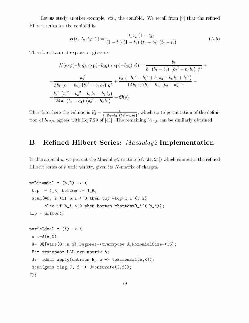
Let us study another example, viz., the conifold. We recall from [9] that the refined

Hilbert series for the conifold is

H(t1, t2, t3; C) =t1 t2 (1 − t3)

(1 − t1) (1 − t2) (t1 − t3) (t2 − t3). (A.5)

Therefore, Laurent expansion gives us

H(exp(−b1q), exp(−b2q), exp(−b3q); C) =b3

b1 (b1 − b3)(b2

2 − b2 b3

)q3

+

+b3

2

2 b1 (b1 − b3)(b2

2 − b2 b3

)q2

+b3

(−b1

2 − b22 + b1 b3 + b2 b3 + b3

2)

12 b1 b2 (b1 − b3) (b2 − b3) q−

−b32(b1

2 + b22 − b1 b3 − b2 b3

)

24 b1 (b1 − b3)(b2

2 − b2 b3

) + O(q)

Therefore, here the volume is V3 = b3b1 (b1−b3) (b2

2−b2 b3), which up to permutation of the defini-

tion of b1,2,3, agrees with Eq 7.29 of [41]. The remaining V2,1,0 can be similarly obtained.

B Refined Hilbert Series: Macaulay2 Implementation

In this appendix, we present the Macaulay2 routine (cf. [21, 24]) which computes the refined

Hilbert series of a toric variety, given its K-matrix of charges.

toBinomial = (b,R) -> (

top := 1_R; bottom := 1_R;

scan(#b, i->if b_i > 0 then top =top*R_i^(b_i)

else if b_i < 0 then bottom =bottom*R_i^(-b_i));

top - bottom);

toricIdeal = (A) -> (

n :=#(A_0);

R= QQ[vars(0..n-1),Degrees=>transpose A,MonomialSize=>16];

B:= transpose LLL syz matrix A;

J:= ideal apply(entries B, b -> toBinomial(b,R));

scan(gens ring J, f -> J=saturate(J,f));

J);

79

The input is the g +2 by E matrix K and the output of the command toricIdeal(K)

is the refined Hilbert series for the coherent component IrrF ♭ weighted by all the g+2 charges

(chemical potentials). The algorithm can be easily generalized to compute the Hilbert series

depending on only one, or fewer, charges.

C Refined Hilbert Series using Molien Formula

In this Appendix we give an explicit example of computation of the refined Hilbert series

using the Molien formula. The method works well for quivers with relatively small number

of fields.

Consider the example of C3/Z2 × Z2. The Hilbert series depending on one parameter

t was computed in §2.1.6 from the symplectic quotient description with charges (2.31). To

highlight the result for the refined Hilbert series we will exploit the full symmetry of the

moduli space. The symmetry of the master space can be readily determined to be SU(2)3 ×U(1)3, the three SU(2)’s coming from repetition of columns in the charge matrix (2.31). This

is another example of the general phenomenon related to the existence of hidden symmetries

which is discussed in detail in §4.

For now, we want to learn how to compute the refined Hilbert series using (2.25). To

this purpose we introduce nine homogeneous variables yα, α = 1, ..., 9 acted on by (C∗)3 with

charges Qi given by the rows of the matrix (2.31). The Molien formula (2.25) then reads

H(y, IrrF ♭C3/Z2×Z2

) =∫

drdwdsrws

1(1−

y1r

w)(1−y2r

s)(1−y3w

s)(1−y4r)(1−y5r)(1−y6w)(1−y7w)(1−y8s)(1−y9s).

(C.6)

The result of the three integrations is a lengthy rational expression that we do not report

here; it depends on 6 independent quantities that can be matched with the six chemical

potentials ti by solving (2.26). In this case we can use the SU(2)3 × U(1)3 symmetry and

introduce a set of adapted chemical potentials respecting the symmetry of the matrix Q:

{y1, y2, y3, y4, y5, y6, y7, y8, y9} = {t1, t2, t3, z, 1/z, y, 1/y, x, 1/x} . (C.7)

The three charges ti parameterize the R-charge and the two non-anomalous flavor U(1)

symmetries of the theory; these are obtained by assigning a different chemical potential to

the three external perfect matchings in the dimer description as discussed in §2.1.7. The

variables x, y, z are the chemical potentials for the Cartan subgroup of SU(2)3 and the refined

80

Hilbert series can be then computed as

H(t1, t2, t3, x, y, z, IrrF ♭C3/Z2×Z2

) = P (t1, t2, t3, x, y, z)PE [t1[0, 1, 1] + t2[1, 0, 1] + t3[1, 1, 0]] ,

(C.8)

with

P (t1, t2, t3, x, y, z) = 1 − t21 − t22 − t23 + 2t1t2t3 + 2t21t22t

23 − t1t

32t

33 − t31t2t

33 − t31t

32t3 + t31t

32t

33

+ [0, 1, 1] (−t2t3 + t1t22 + t1t

23 − t21t2t3 − t1t

22t

23 + t21t

32t3 + t21t2t

33 − t31t

22t

23)

+ [1, 0, 1] (−t1t3 + t21t2 + t2t23 − t1t

22t3 − t21t2t

23 + t31t

22t3 + t1t

22t

33 − t21t

32t

23)

+ [1, 1, 0] (−t1t2 + t21t3 + t22t3 − t1t2t23 − t21t

22t3 + t31t2t

23 + t1t

32t

23 − t21t

22t

33)

+ [2, 0, 0] (t1t2t3 − t22t23 − t31t2t3 + t21t

22t

23)

+ [0, 2, 0] (t1t2t3 − t21t23 − t1t

32t3 + t21t

22t

23)

+ [0, 0, 2] (t1t2t3 − t21t22 − t1t2t

33 + t21t

22t

23) ,

(C.9)

where [n, m, l] is the character of the representation of dimension (n+1, m+1, l+1) of SU(2)3

expressed in the variables x, y, z with the specified order. For example, [1, 0, 0] = x + 1/x.

The plethystic exponential PE in the above is defined in §2.3.3 which we recall is such

that for polynomials or power series f(t) with f(0) = 0, it is given by

PE [f(t)] = exp

(∞∑

k=1

f(tk)

k

)

. (C.10)

In our case, the plethystic exponential counts all possible symmetric products of the twelve

elementary fields organized as the [0, 1, 1], [1, 0, 1] and [1, 1, 0] representations of SU(2)3. The

symmetry of the master space is manifest in the expression of the refined Hilbert series; this

is the subject of §4. Notice also the remarkable palindromic symmetry of the numerator

of the refined Hilbert series as a polynomial in three variables t1, t2, t3 under the exchange

ti1tj2t

k3 ↔ t3−i

1 t3−j2 t3−k

3 . This point is discussed in detail in §2.3.1.

On the practical side, it is sometimes convenient to perform the integration in the

Molien formula before substituting the expression of the dummy variables yα in terms of ti

since in this way there is no ambiguity in the integration: the contour integral is performed

on unit circles and take contributions from the poles inside the unit circles, where we consider

all |yα| < 1.

81

References

[1] S. Bradlow, G. Daskalopoulos, R. Wentworth, “Birational Equivalences of Vortex

Moduli,” arXiv:alg-geom/9304001. Topology 35 (1996) 731–748.; A. Bertram, G.

Daskalopoulos, R. Wentworth, “Gromov Invariants for Holomorphic Maps from Rie-

mann Surfaces to Grassmannians,” arXiv:alg-geom/9306005, J. Amer. Math. Soc. 9

(1996) 529–571.

M. Thaddeus, “Geometric invariant theory and flips,” J. Amer. Math. Soc. 9 (1996)

691-723.

C. Okonek, A. Teleman, “Master Spaces and the Coupling Principle: From Geometric

Invariant Theory to Gauge Theory,” Commun. Math. Phys. 205, 437 – 458 (1999).

[2] D. Berenstein, “Reverse geometric engineering of singularities,” JHEP 0204, 052 (2002)

[arXiv:hep-th/0201093].

[3] M. R. Douglas, B. R. Greene and D. R. Morrison, “Orbifold resolution by D-branes,”

Nucl. Phys. B 506, 84 (1997) [arXiv:hep-th/9704151].

[4] C. Beasley, B. R. Greene, C. I. Lazaroiu and M. R. Plesser, “D3-branes on partial

resolutions of abelian quotient singularities of Calabi-Yau threefolds,” Nucl. Phys. B

566, 599 (2000) [arXiv:hep-th/9907186].

[5] B. Feng, A. Hanany and Y. H. He, “D-brane gauge theories from toric singularities and

toric duality,” Nucl. Phys. B 595, 165 (2001) [arXiv:hep-th/0003085].

B. Feng, A. Hanany and Y. H. He, “Phase structure of D-brane gauge theories and toric

duality,” JHEP 0108, 040 (2001) [arXiv:hep-th/0104259].

[6] A. Hanany and K. D. Kennaway, “Dimer models and toric diagrams,”

arXiv:hep-th/0503149.

S. Franco, A. Hanany, K. D. Kennaway, D. Vegh and B. Wecht, “Brane dimers and

quiver gauge theories,” JHEP 0601, 096 (2006) [arXiv:hep-th/0504110].

B. Feng, Y. H. He, K. D. Kennaway and C. Vafa, “Dimer models from mirror symmetry

and quivering amoebae,” arXiv:hep-th/0511287.

S. Franco and D. Vegh, “Moduli spaces of gauge theories from dimer models: Proof of

the correspondence,” JHEP 0611, 054 (2006) [arXiv:hep-th/0601063].

82

http://arXiv.org/abs/alg-geom/9304001

http://arXiv.org/abs/alg-geom/9306005

http://arXiv.org/abs/hep-th/0201093









[7] S. Franco, A. Hanany, D. Martelli, J. Sparks, D. Vegh and B. Wecht, “Gauge theories

from toric geometry and brane tilings,” JHEP 0601 (2006) 128 [arXiv:hep-th/0505211].

A. Hanany and D. Vegh, “Quivers, tilings, branes and rhombi,” arXiv:hep-th/0511063.

[8] K. D. Kennaway, “Brane Tilings,” Int. J. Mod. Phys. A 22, 2977 (2007) [arXiv:0706.1660

[hep-th]].

[9] S. Benvenuti, B. Feng, A. Hanany and Y. H. He, “Counting BPS operators in gauge

theories: Quivers, syzygies and plethystics,” arXiv:hep-th/0608050.

B. Feng, A. Hanany and Y. H. He, “Counting gauge invariants: The plethystic program,”

JHEP 0703, 090 (2007) [arXiv:hep-th/0701063].

[10] A. Butti, D. Forcella and A. Zaffaroni, “Counting BPS baryonic operators in CFTs with

Sasaki-Einstein duals,” JHEP 0706, 069 (2007) [arXiv:hep-th/0611229].

[11] D. Forcella, A. Hanany and A. Zaffaroni, “Baryonic generating functions,”

arXiv:hep-th/0701236.

[12] A. Butti, D. Forcella, A. Hanany, D. Vegh and A. Zaffaroni, “Counting Chiral Operators

in Quiver Gauge Theories,” arXiv:0705.2771 [hep-th].

[13] D. Forcella, “BPS Partition Functions for Quiver Gauge Theories: Counting Fermionic

Operators,” arXiv:0705.2989 [hep-th].

[14] D. Forcella, A. Hanany, Y.-H. He and A. Zaffaroni, “Mastering the Master Space,” To

appear.

[15] W. Fulton, “Introduction to Toric Varieties,” (AM-131) by Fulton, Princeton University

Press, 1993.

[16] A. Hanany and A. Zaffaroni, “On the realization of chiral four-dimensional gauge the-

ories using branes,” JHEP 9805, 001 (1998) [arXiv:hep-th/9801134].

A. Hanany and A. M. Uranga, “Brane boxes and branes on singularities,” JHEP 9805,

013 (1998) [arXiv:hep-th/9805139].

[17] T. Muto and T. Tani, “Stability of quiver representations and topology change,” JHEP

0109, 008 (2001) [arXiv:hep-th/0107217].

[18] T. Sarkar, “D-brane gauge theories from toric singularities of the form C(3)/Gamma

and C(4)/Gamma,” Nucl. Phys. B 595, 201 (2001)

83



http://arXiv.org/abs/0706.1660










[19] H. F. Blichfeldt, “Finite Collineation Groups,” The Univ. Chicago Press, Chicago, 1917.

A. Hanany and Y. H. He, “A monograph on the classification of the discrete subgroups

of SU(4),” JHEP 0102, 027 (2001) [arXiv:hep-th/9905212].

[20] J. Gray, Y. H. He, V. Jejjala and B. D. Nelson, “Exploring the vacuum geometry of

N = 1 gauge theories,” Nucl. Phys. B 750, 1 (2006) [arXiv:hep-th/0604208].

[21] D. Grayson and M. Stillman, “Macaulay 2, a software system for research in algebraic

geometry,” Available at http://www.math.uiuc.edu/Macaulay2/

[22] J. Gray, Y.-H. He, A. Ilderton and A. Lukas, “STRINGVACUA, A Mathematica Pack-

age for Studying Vacuum Configurations in String Phenomenology”, [arXiv:0801.1508

[hep-th]]

[23] B. Sturmfels, “Grobner Bases and Convex Polytopes,” American Mathematical Society,

Providence, RI, 1996

[24] David Eisenbud, Daniel R. Grayson, Michael E. Stillman, and Bernd Sturmfels

Ed.,Chapter Algorithms for the Toric Hilbert Scheme in “Computations in algebraic

geometry with Macaulay 2,” Springer-Verlag 2001.

[25] D. Cox, “The homogeneous coordinate ring of a toric variety,” J. Algebraic Geom. 4

(1995) 17-50.

[26] P. Pouliot, “Molien function for duality,” JHEP 9901, 021 (1999)


F. A. Dolan, “Counting BPS operators in N = 4 SYM,” Nucl. Phys. B 790, 432 (2008)

[arXiv:0704.1038 [hep-th]].

[27] G. Birkhoff, “Tres observaciones sobre el algebra lineal,” Univ. Nac. Tucuman Rev. Ser.

A, vol. 5, pp. 147-151, 1946.

J. von Neumann, “A certain zero-sum two-person game equivalent to the optimal as-

signment problem,” in Contributions to the Theory of Games. Princeton, NJ: Princeton

Univ. Press, 1953, vol. 2, pp. 5-12.

[28] A. Butti and A. Zaffaroni, “R-charges from toric diagrams and the equivalence of a-

maximization and Z-minimization,” JHEP 0511 (2005) 019 [arXiv:hep-th/0506232].

84



http://www.math.uiuc.edu/Macaulay2/





[29] A. Butti and A. Zaffaroni, “From toric geometry to quiver gauge theory: The

equivalence of a-maximization and Z-minimization,” Fortsch. Phys. 54 (2006) 309


[30] D. R. Morrison and M. R. Plesser, “Non-spherical horizons. I,” Adv. Theor. Math. Phys.

3, 1 (1999) [arXiv:hep-th/9810201].

[31] A. Hanany and C. Romelsberger, “Counting BPS operators in the chiral ring of N = 2

supersymmetric gauge theories or N = 2 braine surgery,” arXiv:hep-th/0611346.

[32] B. Feng, A. Hanany, Y. H. He and A. M. Uranga, “Toric duality as Seiberg duality and

brane diamonds,” JHEP 0112, 035 (2001) [arXiv:hep-th/0109063].

[33] S. Franco and A. Hanany, “Toric duality, Seiberg duality and Picard-Lefschetz trans-

formations,” Fortsch. Phys. 51, 738 (2003) [arXiv:hep-th/0212299].

[34] B. Feng, S. Franco, A. Hanany and Y. H. He, “Unhiggsing the del Pezzo,” JHEP 0308,

058 (2003) [arXiv:hep-th/0209228].

[35] B. Feng, S. Franco, A. Hanany and Y. H. He, “Symmetries of toric duality,” JHEP

0212, 076 (2002) [arXiv:hep-th/0205144].

[36] R. Stanley, “Hilbert functions of graded algebras,” Adv. Math. 28 (1978), 57-83.

[37] S. Franco, A. Hanany and P. Kazakopoulos, “Hidden exceptional global symmetries in

4d CFTs,” JHEP 0407, 060 (2004) [arXiv:hep-th/0404065].

[38] J. Harris and W. Fulton, “Representation theory,” no. 129 in GTM, Springer-Verlag,

New York, NY, 1991.

[39] A. Butti, D. Forcella and A. Zaffaroni, “Deformations of conformal theories and non-

toric quiver gauge theories,” JHEP 0702 (2007) 081 [arXiv:hep-th/0607147].

[40] M. Wijnholt, “Large volume perspective on branes at singularities,” Adv. Theor. Math.

Phys. 7, 1117 (2004) [arXiv:hep-th/0212021].

[41] D. Martelli, J. Sparks and S. T. Yau, “Sasaki-Einstein manifolds and volume minimi-

sation,” arXiv:hep-th/0603021.

85












The master space of Script N= 1 gauge theories

Documents

Transcript of The master space of Script N= 1 gauge theories