arX

iv:h

ep-t

h/97

1119

1v3

22

Jan

1998

hep-th/9711191CBPF-NF-052/97UFES–DF–OP97/2

On the Non-Renormalization Properties

of Gauge Theories

with a Chern-Simons Term

Oswaldo M. Del Cima(a),(b),1, Daniel H.T. Franco(b),2,

Jose A. Helayel-Neto(b) and Olivier Piguet(c),2,3,4

(a) Pontifıcia Universidade Catolica do Rio de Janeiro (PUC-RIO),Departamento de Fısica,

Rua Marques de Sao Vicente, 225 - 22453-900 - Rio de Janeiro - RJ - Brazil.

(b) Centro Brasileiro de Pesquisas Fısicas (CBPF),Departamento de Teoria de Campos e Partıculas (DCP),

Rua Dr. Xavier Sigaud 150 - 22290-180 - Rio de Janeiro - RJ - Brazil.

(c) Universidade Federal do Espırito Santo (UFES),CCE, Departamento de Fısica,

Campus Universitario de Goiabeiras - 29060-900 - Vitoria - ES - Brazil.

E-mails: delcima@tph73.tuwien.ac.at, dfranco@cbpfsu1.cat.cbpf.br,helayel@cbpfsu1.cat.cbpf.br, piguet@cce.ufes.br.

1Current address: Institut fur Theoretische Physik, Technische Universitat Wien, Wiedner Haupt-strasse 8-10 - A-1040 - Vienna - Austria.

2Supported by the Conselho Nacional de Desenvolvimento Cientıfico e Tecnologico (CNPq).3Supported in part by the Swiss National Science Foundation.4On leave of absence from Departement de Physique Theorique, Universite de Geneve, 24 quai E.

Ansermet - CH-1211 - Geneve 4 - Switzerland.

1

Abstract

Considering three-dimensional Chern-Simons theory, either coupled to matter orwith a Yang-Mills term, we show the validity of a trace identity, playing the role ofa local form of the Callan-Symanzik equation, in all orders of perturbation theory.From this we deduce the vanishing of the β-function associated to the Chern-Simonscoupling constant and the full finiteness in the case of the Yang-Mills Chern-Simonstheory. The main ingredient in the proof of the latter property is the noninvarianceof the Chern-Simons form under the gauge transformations. Our results hold forthe three-dimensional Chern-Simons model in a general Riemannian manifold.

1 Introduction

Topological field theories (see [1] for a general review and references) are a class of gaugemodel interesting from a physical point of view. In particular, their observables are oftopological nature. An important topological model that has received much attention inthe last years is the Chern-Simons model in three dimensions [2, 3, 4]. In contrast tothe usual Yang-Mills gauge theories, Chern- Simons theories, which include the case ofthree-dimensional gravity [5, 6], have some remarkable features. Besides their relevancein connection with the possibility of getting nonperturbative results more easily and theirrelation with the two-dimensional conformal field theories [7], they show very interestingperturbative features such as ultraviolet finiteness [5, 6, 8]. A complete and rigorousproof of the latter property has been given in [9] for D = 1 + 2 Chern-Simons theories inthe Landau gauge. In the more general case where these models are coupled to matterfields, the Chern-Simons coupling constant keeps unrenormalized, the corresponding β-function remaining vanishing. This has been rigorously proved in [10] for the AbelianChern-Simons theory coupled to scalar matter fields. For the nonabelian theory coupledto spinorial matter fields, an argument based on the assumed existence of an invariantregularization has been proposed by the authors of [11].

On the other hand, there exist studies in the literature concerning the Yang-MillsChern-Simons (YMCS) theory [12, 13, 14, 15]. In particular the finiteness at one loopwas detected in refs. [12, 14], where explicit expressions for one-loop radiative correctionscan be found. Later on in [15] has been showed that no UV divergences arise up totwo-loops in perturbation theory, combining this result with finiteness by power countingat higher loops to argument that theory is finite at any perturbative order. Recently,similar arguments has been used to prove the finiteness for the N = 1 supersymmetricversion of the YMCS theory [16]. A cohomological study of N = 2 YMCS theory ina nonsupersymmetric gauge has been performed in [17], where a partial proof of thefiniteness is given.

Two recent papers [18, 19] have shown the equivalence of the YMCS theory with apure Cherns-Simons theory, in the classical approximation. One of our results, namelythe complete ultraviolet finiteness of the YMCS, although proved in perturbation theoryonly, indicates that this equivalence could hold for the full quantum theory. Let usfinally mention that Ref. [19], appeared after completion of the present paper, beyond

2

of expanding the classical results of [18] and arguing in favour of a possible quantumgeneralization, shows that, at the quantum level, the YMCS theory is finite up to possiblefield amplitude renormalizations.

Our first purpose in this paper is to give a rigorous proof of the vanishing of the Chern-Simons β-function in the presence of general scalar and spinorial matter, introduced inthe most general way compatible with renormalizability. We shall avoid the necessityof invoking a particular regularization procedure, by using the “algebraic” method ofrenormalization [20], which only relies on general theorems of renormalization theory.We think indeed that, due to the presence of the antisymmetric Levi-Civita tensor, it isdifficult to establish an invariant regularization without encountering problems at some orother stage of the argument. Thus, to the contrary of the authors of [11], we shall neitherassume an invariant regularization nor the explicit “multiplicative renormalizability” atthe level of the Lagrangian which would follow from this assumption.

Our first result generalizes that of [10], the gauge group being now an arbitrary com-pact Lie group. We exploit the scaling properties of the theory, described by the Callan-Symanzik equation, which is the anomalous Ward identity for scale invariance. Moreprecisely, as in [10], we make use of a local form of the Callan-Symanzik equation. But,instead of introducing an external dilatation field as in [10], beyond the external metricor dreibein field, we only consider the latter, considered as a source for the BRS invariantenergy-momentum tensor. The conservation of the energy-momentum tensor is expressedthrough the Ward identity which characterizes the invariance of the theory under thediffeomorphisms. Our “local Callan-Symanzik equation” then is the anomalous Wardidentity for the BRS invariant trace of the energy-momentum tensor, the so-called “traceidentity”. As expected [10, 11], the nonrenormalization of the Chern-Simons coupling,which amounts to the vanishing of the corresponding β-function, is traced back to thefact that the integrand of the Chern-Simons action is not BRS invariant but transformsas a total derivative.

Of course the β-functions associated with the other couplings – the self-couplings ofthe matter fields – do not vanish in general.

Our second result is a purely algebraic proof of the all-order, complete finiteness ofthe YMCS theory, using the same techniques, but exploiting the superrenormalizabilityof the model. To our knowledge, up to now, no such algebraic proof had been given. Letus note that, although the proof of finiteness given in [19] confirms our second result inquite an independent way, there are differences which should be noted. First, the resultof [19] is more general than ours since it holds for a more general set of theories, whichare not necessarely power-counting renormalizable. Second, this result holds only up topossible field amplitude renormalizations. However, restricting ourselves to the power-counting renormalizable case, we are also able to show the complete finiteness, includingthe nonrenormalization of the field amplitudes, as it is the case for the pure Chern-Simonstheory [8, 9].

Since we are working with an external dreibein which is not necessary flat, our resultshold for a curved manifold, as long as its topology remains that of flat R3, with asymptoti-cally vanishing curvature. It is the latter two restrictions which allow us to use the general

3

results of renormalization theory, established in flat space. Indeed, we may then expandin the powers of the difference between the curved and flat space dreibeins, this differencebeing considered as an external field in flat space, fastly decreasing asymptotically.

The paper is organized as follows. The Chern-Simons theory coupled to matter, ina curved three-dimensional Riemannian manifold described in terms of external dreibeinand spin connection fields, is introduced in Section 2, together with its symmetries. Therenormalizability of the model is sketched in Section 3, and our argument leading to thevanishing of the Chern-Simons β-function is presented in Section 4. The application ofour techniques to the finiteness of the YMCS theory is presented in section 5, followedby our conclusions. The paper is completed with two Appendices: In the App. A wecompute the classical trace identity whose quantum extension leads to the local form ofthe Callan-Symanzik equation. The App. B recalls some properties of the short distanceWilson expansion which are used in the main text.

2 The Chern-Simons Model Coupled With Matter in

Curved Space-Time

The Classical Action

The gauge field Aaµ(x) lies in the adjoint representation of the gauge group G, a general

compact Lie group with Lie algebra

[Xa, Xb] = ifabcXc .

The scalar matter fields ϕi(x) and the spinor matter fields ΨA(x) are in some representa-tions of G, the generators being represented by the matrices T (ϕ)

a and T (Ψ)a , respectively.

Space-time is a three-dimensional Riemannian manifold M, with coordinates xµ, µ =0, 1, 2. It is described by a dreibein field em

µ (x) and its inverse eµm(x), µ being a world

index and m a tangent space index. The spin connection ωmnµ (x) is not an independent

field, but depend on the dreibein due to the vanishing torsion condition. The metrictensor and its inverse read

gµν (x) = ηmn emµ (x) en

ν (x) , gµν (x) = ηmn eµm (x) eν

n (x) , (2.1)

ηmn being the tangent space flat metric. We denote by e the determinant of emµ .

As explained in the Introduction, we assume the manifold M to be topologicallyequivalent to R3 and asymptotically flat.

The invariances of the theory are:

1) Gauge invariance. The infinitesimal gauge tranformations read – anticipating, wewrite them as BRS transformations, i.e. we replace their infinitesimal parameters by theanticommuting Faddeev-Popov ghost fields ca(x); we also introduce the antighost fields

4

ca(x) and the Lagrange multiplyier fields ba(x) which will be used later on in order todefine the gauge fixing condition –

sAaµ = −Dµc

a ≡ −(

∂µca + fbcaAb

µcc)

, sca = 12fbc

acbcc ,

sΨA

= i caT (Ψ)a A

BΨB , sca = ba ,

sϕi = i caT (ϕ)a i

jϕj , sba = 0 .

(2.2)

The variation of the ghost c is chosen such as to make the BRS operator s nilpotent:

s2 = 0 .

2) Invariance under diffeomorphisms. The infinitesimal diffeomorphisms read

δ(ε)diffFµ = LεFµ = ελ∂λFµ +

(

∂µελ)

Fλ , Fµ = Aaµ, em

µ ,

δ(ε)diffΦ = LεΦ = ελ∂λΦ , Φ = ϕi, ΨA, ba, ca, ca ,

(2.3)

where Lε is the Lie derivative along the vector field εµ(x) – the infinitesimal parameterof the transformation.

3) Local Lorentz invariance. The infinitesimal transformations, with infinitesimal pa-rameters λ[mn], are given by

δ(λ)LorentzΦ =

1

2λmnΩmnΦ , Φ = any field , (2.4)

with Ω[mn] acting on Φ as an infinitesimal Lorentz matrix in the appropriate representa-tion.

The most general classical, power-counting renormalizable action invariant under thediffeomorphisms and local Lorentz transformations, and gauge invariant – i.e. BRS-invariant and independent of the ghost fields – is of the form

Σinv =∫

d3x(

κ εµνρ

(

Aaµ∂νA

aρ +

1

3fabcA

aµA

bνA

cρ

)

+ e(

i ΨAγµDµΨ

A+ 1

2DµϕiDµϕi − V(ϕ, Ψ)

)

)

,(2.5)

with the generalized covariant derivative defined by

DµΦ(x) ≡(

∂µ − i Aaµ(x)T (Φ)

a +1

2ωmn

µ (x)Ωmn

)

Φ(x) . (2.6)

The function V(ϕ, Ψ) defines the selfinteractions of the matter fields and their masses:

V (ϕ, Ψ) =1

6λ ϕ6 +

1

2y ΨΨϕ2 + mass terms + dimensionful couplings , (2.7)

whith the short-hand notation

λ ϕ6 = λijklmnϕiϕjϕkϕlϕmϕn ,

y ΨΨϕ2 = yABmnΨAΨBϕmϕn ,

λ and y being invariant tensors of the gauge group. We do not write explicitly the massterms and the dimensionful couplings since we are interested in the scaling properties inthe high energy-momentum limit.

5

Gauge Fixing

The gauge fixing is of the Landau type. It is implemented by adding to the gauge invariantaction (2.5) the term

Σgf = − s∫

d3x e gµν∂µcaAaν = −

∫

d3x e gµν (∂µbaAaν + ∂µcaDνc

a) , (2.8)

which is BRS invariant due to the nilpotency of s.

Moreover, because of the nonlinearity of some of the BRS transformations (2.2), wehave also to add a term giving their coupling with external fields, the “antifields” A∗µ

a , c∗a,Ψ∗

A, ϕ∗i :

Σext =∫

d3x∑

Φ=Aaµ, ca,ΨA, ϕi

Φ∗sΦ . (2.9)

The antifields are tensorial densities: they transform under the diffeomorphisms as

δ(ε)diffA∗µ

a = LεA∗µa = ∂λ

(

ελA∗µa

)

− (∂λεµ) A∗λ

a

δ(ε)diffΦ∗ = LεΦ

∗ = ∂λ

(

ελΦ∗)

, Φ∗ = c∗a, ϕ∗

i , Ψ∗

A .

Their transformations under local Lorentz symmetry are obvious. They are moreoverBRS invariant.

From now on we consider the total action

Σ = Σinv + Σgf + Σext . (2.10)

The Functional Identities

The various symmetries of the model as well as the gauge fixing we have choosen may beexpressed as functional identities obeyed by the classical action (2.10).

The BRS invariance is expressed through the Slavnov-Taylor identity

S(Σ) =∫

d3x∑

Φ=Aaµ, ca,Ψ

A, ϕi

δΣ

δΦ∗

δΣ

δΦ+ b Σ = 0 , with b =

∫

d3x ba δ

δca. (2.11)

For later use we introduce the linearized Slavnov-Taylor operator

BΣ =∫

d3x∑

Φ=Aaµ, ca,Ψ

A, ϕi

(

δΣ

δΦ∗

δ

δΦ+

δΣ

δΦ

δ

δΦ∗

)

+ b . (2.12)

S and B obey the algebraic identity

BFBFF′ + (BF ′ − b)S(F) = 0 , (2.13)

F and F ′ denoting arbitrary functionals of ghost number zero. From the latter follow

BF S(F) = 0 , ∀ F , (2.14)

6

(BF )2 = 0 if S(F) = 0 . (2.15)

In particular, since the action Σ obeys the Slavnov-Taylor identity, we have the nilpotencyproperty (2.11):

(BΣ)2 = 0 . (2.16)

In addition to the Slavnov-Taylor identity (2.11), the action (2.10) satisfies the followingconstraints:

– the Landau gauge condition:

δΣ

δba

= ∂µ (egµνAaν) , (2.17)

– the “antighost equation”, peculiar to the Landau gauge [21],

GaΣ =∫

d3x

(

δ

δca+ f abccb

δ

δbc

)

Σ = ∆acl , (2.18)

with∆a

cl =∫

d3x(

f abc (A∗µb Acµ − c∗bcc) + iΨ∗T (Ψ)

a Ψ − iϕ∗T (ϕ)a ϕ

)

,

(The right-hand side of (2.18) being linear in the quantum fields will not get renormalized.)

– the Ward identities for the invariances under the diffeomorphisms (2.3) and the localLorentz transformations (2.4):

WdiffΣ =∫

d3x∑

Φ

δ(ε)diffΦ

δΣ

δΦ= 0 , (2.19)

and

WLorentzΣ =∫

d3x∑

Φ

δ(λ)LorentzΦ

δΣ

δΦ= 0 , (2.20)

where the summations run over all quantum and external fields.

The functional operators defined here above, together with the operators

Ga =δ

δca

+ ∂µ

(

egµνδ

δA∗νa

)

,

Warigid =

∫

d3x

∑

φ=A,c,c,b,A∗,c∗

f abcφb

δ

δφc+

∑

Φ=Ψ,ϕ,Ψ∗,ϕ∗

T (Φ)aΦδ

δΦ

.

(2.21)

obey the algebra (2.13), (2.14) and

δS(F)

δba

− BF

(

δF

δba

− ∂µ (egµνAaν)

)

= Ga F , (2.22)

GaS (F) + BFGaF = 0 , (2.23)

GaS (F) + BF

(

GaF − ∆acl

)

= WarigidF , (2.24)

WXS(F) − BFWXF = 0 , X = diff, Lorentz , rigid , (2.25)

7

where F is an arbitrary functional of ghost number zero.

One notes that, since the action Σ (2.10) obeys the Slavnov-Taylor identity (2.11) andthe gauge condition (2.17), the identities (2.22) and (2.24) imply:

– the ghost equation of motionGaΣ = 0 , (2.26)

– the Ward identity expressing the rigid invariance of the theory, i.e. its invariance underthe gauge transformations with constant parameters,

WarigidΣ = 0 . (2.27)

The ghost equation (2.26) implies that the theory depends on the field c and on theantifield A∗µ through the combination

A∗µa = A∗µ

a + egµν∂ν ca . (2.28)

3 Renormalizability

We face now the problem of showing that all the constraints defining the classical theoryalso hold at the quantum level, i.e., that we can construct a renormalized vertex functional

Γ = Σ + O (h) , (3.1)

obeying the same constraints and coinciding with the classical action at order zero in h.

As announced in the Introduction, the proof of renormalizability will be valid for man-ifolds which are topologically equivalent to a flat manifold and which admit an asymp-totically flat metric. It is only in this case that one can expand in powers of em

µ = emµ −

δmµ , considering em

µ as a classical background field in flat R3, and thus make use of thegeneral theorems of renormalization theory actually proved for flat space-time [22, 23].

Power-Counting

The first point to be checked is power-counting renormalizability. It follows from the factthat the dimension of the action is bounded by three5. The ultraviolet dimension as wellas the ghost number and the Grassmann parity of all fields and antifields are collected inTable 1.

5The ultraviolet dimension of the fields coincide with their canonical dimensions. They determinethe ultraviolet power-counting. If there are massless fields in the theory, one should take special careof the infrared convergence [24]. We shall not insist on this, since we are interested here in the purelyultraviolet problem of the nonrenormalization of the Chern-Simons coupling. We shall simply assumethat no “infrared anomaly” or “radiative mass generation” [25] occurs.

8

Aµ Ψ ϕ b c c A∗µ Ψ∗ ϕ∗ c∗ e aµ

d 1 1 1/2 1 0 1 2 2 5/2 3 0ΦΠ 0 0 0 0 1 −1 −1 −1 −1 −2 0GP 0 1 0 0 1 1 1 0 1 0 0

Table 1: Ultraviolet dimension d, ghost number ΦΠ and Grassmann parity GP .

Renormalized Functional Identities

The second point to be discussed is that of the functional identities which have to beobeyed by the vertex functional.

The gauge condition (2.17), ghost equation (2.26), antighost equation (2.18) as wellas rigid gauge invariance (2.27) can easily be shown to hold at all orders, i.e., are notanomalous [20]. The validity to all orders of the Ward identities of diffeomorphisms andlocal Lorentz will be assumed in the following: the absence of anomalies for them has beenproved in refs. [26, 28] for the class of manifolds we are considering here. Therefore weshall be working in the space of diffeomorphism and local Lorentz invariant functionals.

It remains now to show the possibility of implementing the Slavnov-Taylor identity(2.11) for the vertex functional Γ. As it is well known [20], this amounts to study thecohomology of the nilpotent operator BΣ, defined by (2.12), in the space of the localintegral functionals ∆ of the various fields involved in the theory. This means that wehave to look for solutions of the form

∆ = ∆cohom + BΣ∆ , (3.2)

for the equationBΣ∆ = 0 . (3.3)

∆cohom represents the cohomology, i.e. the “nontrivial” part of the general solution: itcannot be written as a BΣ-variation of a local integral functional ∆.

The solutions ∆ with ghost number 0 represent the arbitrary invariant countertermsone can add to the action at each order of perturbation theory. The nontrivial ones cor-respond to a renormalization of the physical parameters: coupling constants and masses,whereas the trivial ones correspond to nonphysical field redefinitions.

The nontrivial solutions with ghost number 1 are the possible gauge anomalies.

In both cases, power-counting renormalizability restricts the dimension of the intgrandof ∆ to 3. Moreover, the constraints (2.17 – 2.20), (2.26) and (2.27), valid now for thevertex functional Γ, imply for ∆ the conditions

(1)δ

δba

∆ = 0 , (2)∫

d3xδ

δ ca∆ = 0 , (3) Ga∆ = 0 ,

(4) WX∆ = 0 , X = diff., Lorentz , rigid .(3.4)

It has been proven in quite generality [27, 28] that in such a gauge theory the coho-

9

mology in the sector of ghost number one is independent of the external fields6. We canthus restrict the field dependence of ∆ to Aµ, c, ϕ, and Ψ – the dependence on c beingthrough its derivatives due to the second of the constraints (3.4).

Beginning with the anomalies (sector of ghost number 1), one knows [26, 28] that,in three dimensions, the cohomology in this sector is empty, up to possible terms inthe Abelian ghosts. They however can be seen, by using the arguments of [29], not tocontribute to the anomaly, due to the freedom or soft coupling of the Abelian ghosts. Wethus conclude to the absence of gauge anomaly, hence to the validity of the Slavnov-Tayloridentity (2.11) to all orders for the vertex functional Γ.

Going now to the sector of ghost number 0, i.e. looking for the arbitrary invariantcounterterms which can be freely added to the action at each order, we find that thenontrivial part of ∆ admits the general representation

∆phys. =

(

zκκ∂

∂κ+ zλ λ

∂

∂λ+ zy y

∂

∂y

)

Σ , (3.5)

where we have only kept the terms of dimension 3 (the lower dimension ones having beingneglected). We have also neglected terms such as

∫

d3x e RΦ2, which do not contributein the limit of flat space. The coefficients zλ and zy are invariant tensors, such as thecoupling λ and y in (2.7).

For the trivial part, we find:

BΣ∆ = (zANA + zΨNΨ + zϕNϕ)Σ , (3.6)

with

NAΣ = (NA − NA∗ − Nb − Nc)Σ = BΣ

∫

d3xA∗µa Aa

µ ,

NΨΣ = (NΨ + NΨ − NΨ∗ − NΨ∗) Σ = −BΣ

∫

d3x(

Ψ∗AΨA + ΨAΨ∗

A

)

,

NϕΣ = (Nϕ − Nϕ∗) Σ = BΣ

∫

d3xϕ∗iϕi ,

(3.7)

where we have introduced the counting operators

NΦ =∫

d3x Φδ

δ Φ, Φ = any field . (3.8)

Eqs. (3.5) and (3.6 – 3.7) make manifest the physical renormalizations, which affect thephysical parameters such as the coupling constants (and the masses), on the one hand,and the nonphysical renormalizations, which correspond to a mere redefinition of the fieldvariables, on the other hand.

This concludes the proof of the renormalizability of the model: all functional identi-ties hold without anomaly and the arbitrary renormalizations only affect the parametersdefined by the initial classical theory.

6The proof is valid for any semi-simple gauge group. But if the gauge group contains Abelian factors,the cohomology in the sector of ghost number one may depend on the external fields [27, 28]. However,it can be shown [29] that such terms cannot contribute to the gauge anomaly due to the Abelian ghostfields being free or at most softly coupled.

10

Callan-Symanzik Equation

The latter renormalization properties are summarized in the Callan-Symanzik equation,which results from the expansion of the invariant insertion defined by

DΓ =∑

all dimensionful parameters µ

µ∂Γ

∂ µ,

in the quantum basis defined by (3.5) and (3.6) – Σ being replaced there by Γ:

(D + βκ∂κ + βy∂y + βλ∂λ − γANA − γΨNΨ − γϕNϕ) Γ ∼ 0 , (3.9)

where ∼ means equality up to mass terms and dimensionful couplings, the terms con-tribuiting which vanish in the flat limit being neglected, too.

The aim of the next and last section is to prove that βκ is vanishing.

4 Nonrenormalization of the Chern-Simons

Coupling

In order to get more deeply into the scaling properties of the present theory, we need alocal form of the Callan-Symanzik equation. This will allow us to exploit the fact thatthe integrand of the Chern-Simons term in the action is not gauge invariant, although itsintegral is. Such a local form of the Callan-Symanzik equation is provided by the “traceidentity”.

In order to derive the latter, let us first introduce the energy-momentum tensor, definedas the following tensorial quantum insertion obtained as the derivative of the vertexfunctional with respect to the dreibein:

Θ µν · Γ = e−1e m

ν

δΓ

δe mµ

. (4.1)

From the diffeomorphism Ward identity (2.19), follows the covariant conservation lawof the energy-momentum tensor:

e∇µ [Θ µν (x) · Γ] = wν (x) Γ + ∇µw

µν (x) Γ , (4.2)

where ∇µ is the covariant derivative with respect to the diffeomorphisms. The right handside is an equation of motion, the functional differential operators wλ (x) and wν

µ (x)being given by (A.2) and (A.3), respectively.

The trace Θ µµ (x) ·Γ turns out to be vanishing, up to total derivatives, mass terms and

dimensionful couplings, in the classical approximation, due to the field equations, whichmeans that (4.1) is the improved energy-momentum tensor. This is shown in AppendixA where we have indeed derived, for the classical theory, the equation

w (x) Σ ∼ ∂µ Λµ (x) , (4.3)

11

or, equivalently:eΘµ

µ(x) ∼ wtrace(x)Σ + ∂µΛµ(x) , (4.4)

with

w = e mµ

δ

δe mµ

− wtrace , (4.5)

wtrace =1

2ϕ

δ

δϕ−

1

2ϕ∗

δ

δϕ∗+ Ψ

δ

δΨ+ Ψ

δ

δΨ− Ψ∗

δ

δΨ∗− Ψ∗

δ

δΨ∗+ ca δ

δca+ ba δ

δba, (4.6)

andΛµ = e iΨγµΨ + eϕ∇µϕ − s (e gµν cAν) . (4.7)

The symbol ∼ in (4.3) and (4.4) again means equality up to mass terms and dimensionfulcouplings.

Let us now look for the quantum version of the trace identity (4.3) or (4.4). We firstobserve that the following commutation relations hold:

[

δ

δba (y), w (x)

]

= −δ (x − y)δ

δba (x),

[

Ga, w (x)]

= 0 ,

[Ga (y) , w (x)] = −δ (x − y)Ga (x) + ∂µδ (x − y)

(

egµν δ

δA∗νa

)

(y) . (4.8)

Let us then define the quantum extension Λµ · Γ of the classical expression (4.7) as avector insertion obeying – beyond the conditions of invariance or covariance under BΓ,Wdiff , WLorentz and Wrigid – the constraints

δ

δba (y)[ Λµ (x) · Γ] = −δ (x − y) e gµνAa

ν , Ga [ Λµ (x) · Γ] = 0 ,

Ga (y) [ Λµ (x) · Γ] = δ (x − y) egµν δΓ

δA∗νa

, (4.9)

already obeyed in the classical limit. Then the divergence ∂µ [Λµ · Γ] will obey the sameconstraints as ω(x)Γ, which read

δ

δba(y)w(x)Γ = −∂µδ(x − y) (e gµνAa

ν) (y) , Gaw(x)Γ = 0 ,

Ga(y)w(x)Γ = ∂µδ(x − y)

(

e gµν δΓ

δA∗νa

)

(y) , (4.10)

and follow from the commutation relations (4.8).

Thus, the dimension 3 insertion ∆ · Γ defined by

w(x)Γ ∼ ∂µ [ Λµ(x) · Γ] + ∆(x) · Γ , (4.11)

– which expresses the quantum corrections to the equation (4.3) – beyond of being in-variant or covariant under BΓ, Wdiff , WLorentz and Wrigid, will obey the homogeneousconstraints

δ

δba(y)[∆(x) · Γ] = 0 , Ga [∆(x) · Γ] = 0 , Ga(y) [∆(x) · Γ] = 0 . (4.12)

12

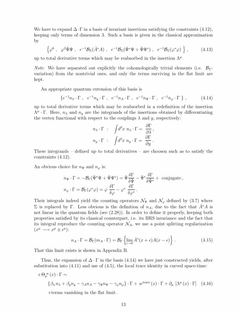
We have to expand ∆ ·Γ in a basis of invariant insertions satisfying the constraints (4.12),keeping only terms of dimension 3. Such a basis is given in the classical approximationby

ϕ6 , ϕ2ΨΨ , e−1BΣ(A∗A) , e−1BΣ(Ψ∗Ψ + ΨΨ∗) , e−1BΣ(ϕ∗ϕ)

, (4.13)

up to total derivative terms which may be reabsorbed in the insertion Λµ.

Note: We have separated out explicitly the cohomologically trivial elements (i.e. BΣ-variation) from the nontrivial ones, and only the terms surviving in the flat limit arekept.

An appropriate quantum extension of this basis is

e−1nλ · Γ , e−1ny · Γ , e−1nA · Γ , e−1nΨ · Γ , e−1nϕ · Γ , (4.14)

up to total derivative terms which may be reabsorbed in a redefinition of the insertionΛµ · Γ. Here, nλ and ny are the integrands of the insertions obtained by differentiatingthe vertex functional with respect to the couplings λ and y, respectively:

nλ · Γ :∫

d3x nλ · Γ =∂Γ

∂λ,

ny · Γ :∫

d3x ny · Γ =∂Γ

∂y.

These integrands – defined up to total derivatives – are choosen such as to satisfy theconstraints (4.12).

An obvious choice for nΨ and nϕ is:

nΨ · Γ = −BΓ(Ψ∗Ψ + ΨΨ∗) = ΨδΓ

δΨ− Ψ∗

δΓ

δΨ∗+ conjugate ,

nϕ · Γ = BΓ(ϕ∗ϕ) = ϕδΓ

δϕ− ϕ∗

δΓ

δϕ∗.

Their integrals indeed yield the counting operators NΨ and Nϕ defined by (3.7) where

Σ is replaced by Γ. Less obvious is the definition of nA, due to the fact that A∗A isnot linear in the quantum fields (see (2.28)). In order to define it properly, keeping bothproperties satisfied by its classical counterpart, i.e. its BRS invariance and the fact thatits integral reproduce the counting operator NA, we use a point splitting regularization(xµ −→ xµ ± ǫµ):

nA · Γ = BΓ(mA · Γ) = BΓ

limǫ→0

A∗(x + ǫ)A(x − ǫ)

. (4.15)

That this limit exists is shown in Appendix B.

Thus, the expansion of ∆ · Γ in the basis (4.14) we have just constructed yields, aftersubstitution into (4.11) and use of (4.5), the local trace identity in curved space-time:

e Θ µµ (x) · Γ ∼

βλ·nλ + βyny − γAnA − γΨnΨ − γϕnϕ · Γ + wtrace (x) · Γ + ∂µ [Λµ (x) · Γ]

+terms vanishing in the flat limit .

(4.16)

13

In order to make the connection between the trace of the energy-momentum tensorand the Callan-Symanzik equation, lets us consider a while the limit of flat space-time,where rigid dilatation symmetry makes sense. In this limit, (4.2) and (4.16) hold withe = 1 and ∇µ = ∂µ. We can therefore define the dilatation current as

[Dµ · Γ]flat = xν [Θ µν (x) · Γ]flat − xν [w µ

ν (x) · Γ]flat − [Λµ (x) · Γ]flat , (4.17)

which, in the classical approximation, is conserved up to mass terms and dimensionfulcouplings (see (A.8)). Thus, for the renormalized theory, in the flat limit, we can writeas usually the Callan-Symanzik equation – which is the Ward identity for anomalousdilatation invariance – as the integral trace identity∫

d3x[

Θ µµ (x) · Γ

]

flat∼ (βκ∂κ + βy∂y + βλ∂λ − γANA − γΨNΨ − γϕNϕ) · Γflat . (4.18)

This observation allows us to identify the coefficients β and γ of the expansion (4.16)with those of the Callan-Symanzik equation (3.9). In particular, the absence of a termcorresponding to the integrand of the Chern-Simons action in the basis (4.14) of invariantlocal operators proves the vanishing of the Chern-Simons β function:

βκ = 0 . (4.19)

5 The Yang-Mills Chern-Simons Theory in Curved

Space-Time

The YMCS action, invariant under the diffeomorphisms and local Lorentz transforma-tions, and gauge invariant – i.e. BRS-invariant – in the Landau gauge, is of the form

Σinv + Σgf =∫

d3x

−e

4F a

µνFaµν + m εµνρ

(

Aaµ∂νA

aρ +

g

3fabcA

aµA

bνA

cρ

)

−∫

d3x e gµν (∂µbaAaν + ∂µcaDνc

a) , (5.1)

where m is a dimensionful coupling constant – the topological mass indeed [12] – and gis the gauge coupling constant, dimensionful, too.

The field strength and covariant derivative are defined as7

F aµν = ∂µA

aν − ∂νA

aµ + gfabcA

bµA

cν , (5.2)

Dµca = ∂µca + gfabcA

bµc

c . (5.3)

The BRS transformations and antighost equation now read

sAaµ = −Dµc

a , sca = g

2fbc

acbcc ,

sca = ba , sba = 0 .(5.4)

7The parametrization of the coupling constant, differing from the one used in the preceding sections,is adapted to the fact that it is now dimensionful.

14

and

GaΣ =∫

d3x

(

δ

δca+ gf abccb

δ

δbc

)

Σ = ∆acl , (5.5)

with

Ga =∫

d3x

(

δ

δca+ g f abccb

δ

δbc

)

, ∆acl = g

∫

d3x f abc (A∗µb Acµ − c∗bcc) ,

The functional identities (2.12), (2.19), (2.20) and the constraints (2.17), (2.26) and(2.27) are unchanged – except for the matter terms which are now absent.

Finally, in order to quantize the system (5.1) we add an action term Σext for thecoupling of the BRS transformations to external fields:

Σext =∫

d3x∑

Φ=Aaµ, ca

Φ∗sΦ . (5.6)

6 Renormalizability and Quantum Scale Invariance

Power-Counting

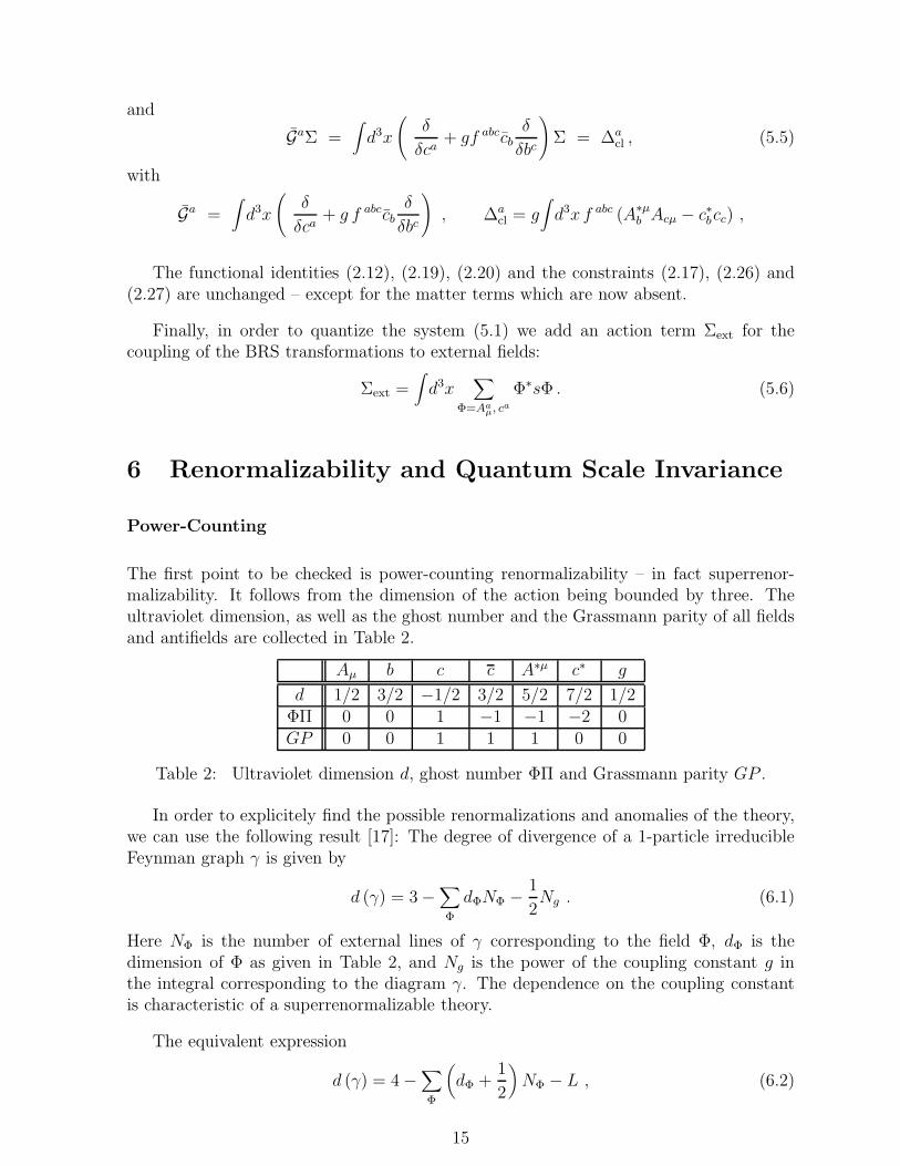
The first point to be checked is power-counting renormalizability – in fact superrenor-malizability. It follows from the dimension of the action being bounded by three. Theultraviolet dimension, as well as the ghost number and the Grassmann parity of all fieldsand antifields are collected in Table 2.

Aµ b c c A∗µ c∗ g

d 1/2 3/2 −1/2 3/2 5/2 7/2 1/2ΦΠ 0 0 1 −1 −1 −2 0GP 0 0 1 1 1 0 0

Table 2: Ultraviolet dimension d, ghost number ΦΠ and Grassmann parity GP .

In order to explicitely find the possible renormalizations and anomalies of the theory,we can use the following result [17]: The degree of divergence of a 1-particle irreducibleFeynman graph γ is given by

d (γ) = 3 −∑

Φ

dΦNΦ −1

2Ng . (6.1)

Here NΦ is the number of external lines of γ corresponding to the field Φ, dΦ is thedimension of Φ as given in Table 2, and Ng is the power of the coupling constant g inthe integral corresponding to the diagram γ. The dependence on the coupling constantis characteristic of a superrenormalizable theory.

The equivalent expression

d (γ) = 4 −∑

Φ

(

dΦ +1

2

)

NΦ − L , (6.2)

15

where L is the number of loops of the diagram, shows that only graphs up to two-looporder are divergent.

In order to apply the known results on the quantum action principle [23] to the presentsituation, one may consider g as an external field of dimension 1

2. Including it in the

summation under Φ, (6.1) gets the same form as in a strictly renormalizable theory:

d (γ) = 3 −∑

Φ=Φ, g

dΦNΦ , with dg =1

2. (6.3)

Thus, including the dimension of g into the calculation, we may state that the dimen-sion of the counterterms of the action is bounded by 3. But, since they are generatedby loop graphs, they are of order 2 in g at least. This means that, not taking now intoaccount the dimension of g, we can conclude that their real dimension is bounded by 2.The same holds for the possible breakings of the Slavnov-Taylor identity.

The absence of anomaly for the Slavnov-Taylor identity holds here in the same wayas previously discussed, in Sect.3.

Let us now look for the arbitrary invariant counterterms which can be freely added tothe action at each order. According to the above discussion the counterterm is at least oforder g2. Thus, the most general expression for the nontrivial part of ∆ reads

∆phys. = zm

∫

d3xm εµνρ

(

Aaµ∂νA

aρ +

g

3fabcA

aµAb

νAcρ

)

, (6.4)

where zm is arbitrary parameter. Expression (6.4) admits the suitable representation

∆phys. = zmm∂

∂mΣ , (6.5)

where Σ is the classical action (2.10). Eq. (6.4) shows that a priori only the parameterm can get radiative corrections. This means that the β-function related to the gaugecoupling constant g is vanishing to all orders of perturbation theory, and the anomalousdimensions of the fields as well. We can just state that the radiative corrections can bereabsorbed through a redefinition of the topological mass only. This concludes the proofof the renormalizability of the theory: all functional identities hold without anomaly andthe renormalizations might only affect the the Chern-Simons coupling, i.e. the topologicalmass m. But the latter turns out to be not renormalized, too. We shall indeed show inthe next Section that the corresponding β-function vanishes.

Quantum Scale Invariance

The argument is very similar to the one presented in Sect. 4. However, the equations (4.3– 4.7) for the classical theory are now replaced by8

w(x)Σ ≡

(

eaµ(x)

δ

δeaµ(x)

− wtrace(x)

)

Σ = Λ(x) , (6.6)

8See appendix A.

16

or, equivalently:eΘµ

µ(x) = wtrace(x)Σ + Λ(x) , (6.7)

with

wtrace (x) = −1

2

(

Aaµ

δ

δAaµ

− A∗µa

δ

δA∗µa

+ ca δ

δca− c∗a

δ

δc∗a

)

+3

2

(

ca δ

δca+ ba δ

δba

)

, (6.8)

and

Λ =m

2εµνλAa

µFaνλ−

g

2fabc

(

e F µν aAbµA

cν + A∗µ aAb

µcc −

1

2c∗ acbcc

)

+ total derivative terms ,

(6.9)Λ being invariant under BΣ.

Note: The latter is the effect of the breaking of scale invariance due to the dimensionfulcouplings. The dimension of Λ – the dimensions of g and m not being taken into account– is lower than three: it is a soft breaking.

The commutation relations (4.8) are changed accordingly into:

[

δ

δba (y), w (x)

]

= −3

2δ (x − y)

δ

δba (x),

[Ga (y) , w (x)] = −3

2δ (x − y)Ga (x) +

3

2∂µδ(x − y)

(

egµν δ

δA∗νa

)

(y) , (6.10)

[

Ga, w(x)]

=1

2

δ

δca(x).

Now the relations (6.10) applied to the vertex functional Γ yield for insertion w(x)Γthe properties

δ

δba(y)w(x)Γ = −

3

2∂µδ(x − y) (e gµνAa

ν) (y) ,

Ga(y)w(x)Γ =3

2∂µδ(x − y)

(

egµν δΓ

δA∗νa

)

(y) , (6.11)

Gaw(x)Γ =1

2

δΓ

δca(x).

where we again use the fact that the constraints (2.17), (2.18) and (2.26) can be maintainedat the quantum level.

The quantum version of (6.6) or (6.7) will be written as

w(x)Γ = Λ(x) · Γ + ∆(x) · Γ , (6.12)

where Λ(x) · Γ is some quantum extension of the classical insertion (6.9), subjected tothe same constraints (6.11) as w(x)Γ. It follows that the insertion ∆ ·Γ defined by (6.12)

17

obeys the homogeneous constraints (4.12), beyond of the usual invariances or covariances.The power-counting dimension of ∆ is 3, but being an effect of the radiative corrections,it possess a factor g2 at least, and thus its effective dimension is at most two – let us recallthat we have attributed power-counting dimension 1/2 to g. It turns out that there isno insertion obeying all these constraints – the Yang-Mills Lagrangian density has termsof dimension 3 (without factor g2) and the Chern-Simons Lagrangian density is not BRSinvariant. Hence ∆ ·Γ = 0: there is no radiative correction to the insertion Λ ·Γ describingthe breaking of scale invariance, and (6.12) becomes

e Θ µµ (x) · Γ = wtrace(x) + Λ(x) · Γ . (6.13)

As in Sect. 4, this local trace identity leads to a Callan-Symanzik equation:

DΓ =∫

d3xΛ(x) · Γ , (6.14)

but now with no radiative effect at all: the β-functions associated to the parameters gand m both vanish, scale invariance remaining affected only by the soft breaking Λ.

7 Conclusions

We have thus achieved the proof of absence of renormalization of the Chern-Simons cou-pling (Eq. (4.19)) for the Chern-Simons theory coupled with matter through a directuse of the nongauge invariance of the Chern-Simons three-form. As a by-product, wehave obtained a trace identity valid in curved space-time (Eq. (4.16)), equivalent to alocal version of the Callan-Symanzik equation (3.9), the result (4.19) being taken intoaccount. The same techniques has allowed us to give a simple proof of the finiteness ofthe Yang-Mills – Chern-Simons theory.

Acknowledgements

We thank Sylvain Wolf for a useful critical reading of the manuscript, and the authorsof Refs. [18, 19] for interesting discussions on the subject of the present paper and ontheir work. This work has been done in parts at the CBPF-DCP, at the Dept. of Physicsof the UFMG and at the the Dept. of Physics of the UFES. We thank all these threeinstitutions for their financial help for travel expenses and for their kind hospitality. Oneof the authors (O.M.D.C.) dedicates this work to his wife, Zilda Cristina, to his daughter,Vittoria, and to his son, Enzo, who is coming.

18

Appendix A: Trace Identity and Dilatation Invariance

for the Classical Theory

Chern-Simons Theory coupled to Matter:

The conservation of the energy-momentum tensor Θ µλ is a consequence of the diffeo-

morphism Ward Identity (2.19) and of the definition (4.1), yielding the following localequation

e∇µΘ µλ (x) = wλ (x) Σ + ∇µw µ

λ (x) Σ , (A.1)

where ∇µ is the covariant derivative with respect to the diffeomorphisms9, with the dif-ferential operators wλ (x) and w µ

λ (x) acting on Σ representing contact terms:

wλ (x) =∑

all fields

(∇λΦ)δ

δΦ, (A.2)

(becoming the translation Ward operator in the limit of flat space), and

w µλ (x) =

A∗µδ

δA∗λ− Aλ

δ

δAµ

− δ µλ

[

ϕ∗δ

δϕ∗+ Ψ∗

δ

δΨ∗+ Ψ∗

δ

δΨ∗+ c∗

δ

δc∗+ A∗µ

δ

δA∗µ

]

.

(A.3)The integral of the trace of the tensor Θ µ

λ ,

∫

d3x e Θ µµ =

∫

d3x e mµ

δΣ

δe mµ

≡ NeΣ , (A.4)

turns out to be an equation of motion – which means that Θ µλ is the improved energy-

momentum tensor. This follows from the identity, which is easily checked by inspectionof the classical action

NeΣ ∼(

NΨ + NΨ +1

2Nϕ + Nb + Nc − NΨ∗ − NΨ∗ −

1

2Nϕ∗

)

Σ , (A.5)

where ∼ means equality up to mass terms and dimensionful couplings, and the NΦ’s arethe counting operators defined by (3.8). Ne is the counting operator of the dreibein fieldem

µ . It is interesting to note that (A.4) is nothing but the Ward identity for rigid Weylsymmetry [30] – broken by the mass terms and dimensionful couplings.

9For a tensor T , such as, e.g., Aµ or δ/δA∗µ:

∇λT µ···ν··· = ∂λT µ···

ν··· + Γλµ

ρTρ···ν··· + · · · − Γλ

ρνT µ···

ρ··· − · · · ,

where the Γ...’s are the Christoffel symbols corresponding to the connexion ωmn

µ . The covariant derivativeof a tensorial density T , such as, e.g., A∗µ or δ/δAµ, is related to that of the tensor e−1T by:

∇λTµ···

ν··· = e∇λ

(

e−1T µ···ν···

)

.

19

Considering the integrand of (A.5), taking (A.4) into account, we may write:

w (x) Σ ∼ ∂µΛµ (x) , (A.6)

with w(x) and Λµ(x) given by (4.6 - 4.7).

We now come to scale invariance, in the flat limit. The classical dilatation current Dµ

can be defined as

Dµ (x) = xλΘ µλ (x) − xλ [w µ

λ (x) Σ] − Λµ (x) . (A.7)

It obeys, up to mass terms, dimensionful couplings and total derivatives, the conser-vation Ward identity, a direct consequence of (A.1) and (A.6):

∂µDµ ∼ w

D(x) Σ , (A.8)

where

wD

(x) = wtrace − w µµ =

∑

all fields

[(dΦ + x · ∂) Φ]δ

δΦ, (A.9)

is the local operator for the scale transformations and dΦ is the dimension of the fieldssurviving in the flat limit (see Table 1).

Yang-Mills Chern-Simons Theory:

The equations (A.1 – A.3) for the conservation of the energy-momentum tensor are un-changed – except the matter terms which are now absent. The expression for the right-hand side of (A.5) is modified into

NeΣ =(

−1

2NA +

1

2NA∗ +

3

2Nb +

3

2Nc −

1

2Nc +

1

2Nc∗

)

Σ +(

m∂m +1

2g∂g

)

Σ . (A.10)

with now a strict equality sign since we keep the contributions from all terms of the action(5.1).

The correspondent of the local identity (A.6) reads

w(x)Σ = Λ(x) ,

with w and Λ given by (6.6 – 6.9)

Finally, as in (A.8), we obtain the broken conservation Ward identity

∂µDµ = w

D(x) Σ + Λ (x) .

The local dilatation operator wD

(x) is given by (A.9), but the dimensions dΦ given inTable 2.

20

Appendix B: Definition of the Bilinear Insertion

(4.15) Through the Wilson-Zimmermann

Short Distance Expansion

The aim is to construct two local insertions mA(x) and nA(x), of ghost number −1 and0, respectively, invariant – or covariant – under BRS, the diffeomorphisms and the locallorentz transformations, and such that

nA(x) · Γ = BΓ [mA(x) · Γ] , (B.1)

and ∫

d3xnA(x) · Γ = NAΓ , (B.2)

where NA is the counting operator defined by (3.7). The classical solution of the problemis given by

mA(x) = A∗µAµ ,

nA(x) = Aµ

(

δΣ

δAµ

+ egµν∂νb

)

− A∗µδΣ

δA∗µ,

(B.3)

with A∗µ defined by (2.28).

In order to find their quantum extensions, let us consider the point splitted insertionsintroduced in (4.15):

meA(x) · Γ = A∗µ(x+)Aµ(x−) · Γ ,

neA(x) · Γ = BΓ [me

A(x) · Γ] ,(B.4)

with xµ± = xµ ± ǫµ, and let us show that the limit ǫ → 0 exists and solves the problem.

The Wilson-Zimmermann short distance expansion [31] yields10

meA(x) · Γ =

∑

K

fK(ǫ)BK(x) · Γ + Re(ǫ, x) , (B.5)

where Re goes to zero in the limit ǫ → 0. The BK(x)’s are all possible renormalizedinsertions (Zimmermann’s normal products [22]) of dimension ≤ 3 (the dimension ofmA), and the coefficients fK(ǫ) have a short distance behaviour

fK(ǫ) ∼ |ǫ|−dK up to logarithmic factors , dK ≤ 3 − dim(BK) .

Taking into account all the constraints which must be obeyed by mA, we see that the listof possible operators BK reduces to quantum extensions of the three following expressions:

B1 = A∗µAµ d1 ≤ 0 ,

B2 = Ψ∗Ψ + ΨΨ∗ d2 ≤ 0 ,

B3 = ϕ∗ϕ d3 ≤ 0 .

(B.6)

10The short distance expansion has been rigorously proved only for theories without massless fields.The extension to massless fields is assumed to hold.

21

Now, we observe that the integral of meA can be written, after partial integration of the

term involving the antighost field c, and use of the gauge condition (2.17), as

∫

d3xmeA(x) · Γ =

∫

d3x

(

A∗µ(x+)Aµ(x−) − c(x+)δΓ

δb(x−)

)

,

which has the well defined limit

∫

d3x

(

A∗µ(x)Aµ(x) − c(x)δΓ

δb(x)

)

, (B.7)

for ǫ → 0. Since there is no total derivative term in the expansion (B.5), we concludefrom this that all three coefficients fK(ǫ) are regular at ǫ = 0. This proves the existenceof the limit

mA(x) · Γ = limǫ→0

meA(x) · Γ , (B.8)

with the integral∫

d3xmA(x) · Γ being equal to the expression (B.7).

The existence of the limit

nA(x) · Γ = limǫ→0

neA(x) · Γ , (B.9)

with the properties (B.1) and (B.2) follows by acting with the BRS operator BΓ on (B.8).

References

[1] D. Birmingham, M. Blau, M. Rakowski and G. Thompson,Phys. Rep. 209 (1991) 129;

[2] A.S. Schwarz, Baku International Topological Conference, Abstracts, vol. 2, p. 345(1987);

[3] E. Witten, Commun. Math. Phys. 117 (1988) 353;Commun. Math. Phys. 118 (1988) 601;

[4] E. Witten, Commun. Math. Phys. 121 (1989) 351;

[5] E. Witten, Nucl. Phys. B311 (1988) 46;

[6] S. Deser, J. McCarthy and Z. Yang, Phys. Lett. B222 (1989) 61;

[7] G. Moore and N. Seiberg, Phys. Lett. B220 (1989) 442;M. Bos and V.P. Nair, Phys. Lett. B223 (1989) 61;J.M.F. Labastida and A.V. Ramallo, Phys. Lett. B227 (1989) 92;S. Emery and O. Piguet, Helv. Phys. Acta 64 (1991) 1256;

[8] E. Guadagnini, M. Martellini and M. Mintchev, Phys. Lett. B227 (1989) 111;Nucl. Phys. B330 (1990) 575;

22

[9] A. Blasi and R. Collina, Nucl. Phys. B345 (1990) 472;F. Delduc, C. Lucchesi, O. Piguet and S.P. Sorella, Nucl. Phys. B346 (1990) 313;C. Lucchesi and O. Piguet, Nucl. Phys. B381 (1992) 281;

[10] A. Blasi, N. Maggiore and S.P. Sorella, Phys. Lett. B285 (1992) 54;

[11] G.A.N. Kapustin and P.I. Pronin, Phys. Lett. B318 (1993) 465;

[12] S. Deser, R. Jackiw and S. Templeton, Ann. Phys. 140 (1982) 372 and 185 (1988)406;

[13] C.P. Martin, Phys. Lett. B241 (1990) 513;

[14] R. Pisarski and S. Rao, Phys. Rev. D32 (1985) 2081;

[15] G. Giavarini, C.P. Martin and F. Ruiz Ruiz, Nucl. Phys. B381 (1992) 222;

[16] F. Ruiz Ruiz and P. van Nieuwenhuizen, Nucl. Phys. B486 (1997) 443;

[17] N. Maggiore, O. Piguet and M. Ribordy, Helv. Phys. Acta 68 (1995) 265;

[18] V.E.R Lemes, C. Linhares de Jesus, C.A.G. Sasaki, S.P. Sorella, L.C.Q. Vilar andO.S. Ventura, “A simple remark on three dimensional gauge theories”, preprintCBPF-NF-050/97, hep-th/9708098, to appear in Phys. Lett. B;

[19] V.E.R. Lemes, C. Linhares de Jesus, S.P. Sorella, L.C.Q. Vilar and O.S. Ven-tura, “Chern-Simons as a geometrical set up for three dimensional gauge theories”,preprint CBPF-NF-078/97, hep-th/9801021;

[20] O. Piguet and S.P. Sorella, “Algebraic Renormalization”, Lecture Notes in Physics,m28, Springer-Verlag, Berlin, Heidelberg, 1995;

[21] A. Blasi, O. Piguet and S. P. Sorella, Nucl. Phys. B356 (1991) 154;

[22] W. Zimmermann, 1970 Brandeis Lectures, Lectures on Elementary Particle andQuantum Field Theory, eds. S. Deser, M. Grisaru and H. Pendleton (MIT PressCambridge); Ann. Phys. (N.Y.) 77 (1973) 536;

[23] J.H. Lowenstein, Phys. Rev. D4 (1971) 2281; Commun. Math. Phys. 24 (1971) 1;Y.M.P. Lam, Phys. Rev. D6 (1972) 2145; Phys. Rev. D7 (1973) 2943;T.E. Clark and J.H. Lowenstein, Nucl. Phys. B113 (1976) 109;

[24] J.H. Lowenstein, Commun. Math. Phys. 47 (1976) 53; “BPHZ Renormalization” inRenormalization Theory, eds. G. Velo and A.S. Wightman (D. Reidel, Dordrecht,1976);

[25] S. Weinberg, Phys. Rev. D7 (1973) 2887;G. Bandelloni, C. Becchi, A. Blasi and R. Collina,Commun. Math. Phys. 67 (1979) 147;W. Bardeen, O. Piguet and K. Sibold, Phys. Lett. B72 (1977) 231;O. Piguet, M. Schweda and K. Sibold, Nucl. Phys. B168 (1980) 337;

[26] F. Brandt, N. Dragon and M. Kreuzer, Nucl. Phys. B340 (1990) 187;

23

[27] G. Barnich and M. Henneaux, Phys. Rev. Lett. 72 (1994) 1558;

[28] G. Barnich, F. Brandt and M. Henneaux, Nucl. Phys. B455 (1995) 357;

[29] G. Bandelloni, C. Becchi, A. Blasi and R. Collina,Ann. Inst. Henri Poincare 28 (1978) 225,255;

[30] A. Iorio, L. O’Raifeartaigh, I. Sachs and C. Wiesendager,Nucl. Phys. B495 (1997) 433;

[31] K.G. Wilson and W. Zimmermann, Commun. Math. Phys. 24 (1972) 87;W. Zimmermann, Ann. Phys. (N.Y.) 77 (1973) 570;

24