Cauchy constraints and particle content of

fourth-order gravity in n dimensions

June 25, 2014

R. Schimming1, M. Abdel-Megied2 and F. Ibrahim3

1 Institut fuer Mathematik und Informatik, E. - M. - Arndt Universitaet Greifswald,D - 17489 Greifswald, Germany

2,3 Mathematics Department, Faculty of Science, Minia University, El-Minia 61111, Egypt

Abstract

The full class of purely metrical gravitational theories in n ≥ 3 dimensions which followsfrom a Lagrangian composed of linear and quadratic curvature terms is analyzed. The typeof the field equations in a suitable gauge is discussed. The principal symbol and the particlecontent of the linearized field equations are investigated. The space + time decompositionand the ADM formalism are used to derive the constraints and evolution equations for thevariational derivative tensor.

Key words: Higher-order-gravity

1991 MSC classification: 83 C 05, 83 D 05

1 Introduction

Fourth-order metrical theories of gravitation have their historical roots in the work of H. Weyl[1] and A. S. Eddington [2], which sought alternatives to Einstein’s general relativity theory [3].Decades later such theories turned out to be semiclassical approximations of quantum gravity.It is not possible here to give an overview on the broad literature on fourth-order gravity. Thepresent paper is influenced by the work of H. A. Buchdahl who was a pioneer in higher-ordergravity and his work especially [8]-[12] is of great importance. H.-J. Schmidt [16], [17] has carrieda systematic investigation of higher-order gravity. K. Mobius [19], [20] pursued an analysis ofquadratic gravity similar to others, but she restricted it to n = 4.

In this paper we study the purely metrical fourth-order theories of gravitation in n ≥ 3dimensions which follow from a Lagrangian

L := Lgrav + 2χLmat, (1.1)

1E-mail: schimmin@mail.uni-greifswald.de2E-mail: abdelmegied@link.net3E-mail: fathyi@hotmail.com

1

2

composed of a gravitational Lagrangian of the form

Lgrav := κR+ c0R2 + c1|Ric|2 + c2|Riem|2, (1.2)

and a matter Lagrangian Lmat, where χ, κ, c0, c1, c2 are real coupling constants, Riem denotesthe Riemannian curvature with covariant components Rαβµν , Ric denotes the Ricci curvaturewith components Rαβ, and R is the scalar curvature of the spacetime metric

g = gαβdxαdxβ (α, β = 0, 1, · · · , n− 1).

We adopt the usual conventions of tensor calculus. In particular, ∇ denotes the Levi-Civitacovariant derivative to g and 2 := gαβ∇α∇β where gαβ := (gαβ)−1. Indices are raised or loweredby means of gαβ or gαβ respectively. We abbreviate |Riem|2 := RαβµνR

αβµν , |Ric|2 := RαβRαβ.

The aim of this paper is to investigate the mathematical structure of quadratic gravity de-termined by (1.1), (1.2) for any dimension n ≥ 3 and for any choice of the coupling constants.Without loss of generality, we can assume κ ≥ 0.

Variation of L with respect to g produces the field equations

Eαβ = χTαβ, (1.3)

where the variational derivative tensor E = Eαβdxαdxβ and the energy-momentum tensor T =

Tαβdxαdxβ are defined by [25]

|det g|12Eαβ :=

δ

δgαβ(|det g|

12Lgrav), (1.4)

|det g|12Tαβ := −2

δ

δgαβ(|det g|

12Lmat), (1.5)

det g := det (gαβ),

and the symbol δ expresses the variational derivatives.

The plan of the paper is as follows. In section 2, we derive the field equations from the La-grangian. In section 3, we calculate and discuss the linearization δEαβ = χδTαβ as field equationsin the variables hαβ = δgαβ, where δ = ∂

∂t · · · |t=0 now denotes the deformation operator. Theprincipal symbol σ4(ξ) of δE = δEαβdx

αdxβ in the general case, the full symbol σ(ξ) for the caseof a flat background, and the particle content on a Minkowski background which follows from aplane-wave ansatz for h = hαβ dx

αdxβ are determined. Moreover, we determine the type of thelinearized field equations in a suitable gauge for Lorentzian or properly Riemannian background.In section 4, Cauchy’s problem is investigated in the following manner: The separation of thefield equations into constraints and evolution equations is carried out by means of coordinatesadapted to a family of spacelike hypersurfaces and the ADM formalism. The structure of theconstraints, ”elliptization” of the constraints is studied in the sense of Petroveskij.

Let us sketch our main results:

-If the background metric g is Lorentzian, the divergence-free gauge ∇βhαβ = 0 is assumed,and the unequalities 4(n − 1)c0 + nc1 + 4c2 6= 0, c1 + 4c2 6= 0 hold, then the linearized fieldequations δEαβ = χδTαβ are hyperbolic. (For our definition of hyperbolicity, cf. Appendix A.)If alternatively, the background metric g is positive definite and again ∇βhαβ = 0, 4(n− 1)c0 +

3

nc1 + 4c2 6= 0, c1 + 4c2 6= 0 are assumed then the linearized field equations are elliptic. (Hereellipticity means that the principal symbol is bijective in the usual sense; cf. Appendix A.)

-If κ > 0, 4(n − 1)c0 + nc1 + 4c2 6= 0, 2c0 + c1 + 2c2 6= 0, then vacuum linearized fourth-ordergravity on a flat background admits a massive spin 0 particle the mass m0 of which is given by

m20 =

(n− 2)κ

4(n− 1)c0 + nc1 + 4c2.

This particle is not a tachyon iff 4(n − 1)c0 + nc1 + 4c2 > 0. If κ > 0, c1 + 4c2 6= 0, then thetheory under consideration admits a massive spin 2 particle the mass m2 of which is given by

m22 = − κ

c1 + 4c2.

This particle is not a tachyon iff c1+4c2 < 0. Finally, if κ > 0 then the theory under considerationadmits a massless spin 2 particle too. More precisely, the fourth-order theory with κ > 0 andEinstein’s gravity show the same content of massless particles.

-If κ = 0, 4(n − 1)c0 + nc1 + 4c2 6= 0, c1 + 4c2 6= 0 then a vacuum linearized purely quadraticgravity, δE = 0 on a flat background does not admit a massive particle. If κ = 0, 4(n− 1)c0 +nc1 + 4c2 6= 0, c1 + 4c2 = 0 then the theory under consideration admits a massive spin 0 particleof any mass m. If κ = 0, If 4(n − 1)c0 + nc1 + 4c2 = 0, c1 + 4c2 6= 0 then the theory underconsideration admits a massive spin 2 particle of any mass m.

-If x0 is a time coordinate and the xi are spacelike coordinates, then the components E00, E0i , Eij

(i, j = 1, · · · , n− 1) of E = Eαβ dxαdxβ have the timelike orders 2, 3, 4 respectively. (Here the

timelike order means the order of the highest derivative with respect to x0 in a given expression.)As a consequence, the field equations Eαβ = χTαβ decompose into constraints E00 = χT 00,E0i = χT 0

i and evolution equations Eij = χTij . We explicitly present the ” timelike principalparts” of E00, E0

i , Eij . Moreover, all fourth-order terms of E = Eαβ dxαdxβ in the lapse function

N and the shift form X = Xidxi are calculated in the framework of the ADM formalism.

-If 2c0 + c1 + 2c2 6= 0, c1 + 4c2 6= 0 then the Cauchy constraints are manifestly elliptic in thelapse function N and the second time derivative of the shift 1-form X, where ”elliptic” is meantin the sense of Petroveskij. We will also present other approaches to ellipticity.

2 The field equations

Let us first fix some notations and conventions. The Riemann curvature tensor Riem withcomponents Rαβµ

ν is introduced through the Ricci identity for a one-form u = uαdxα in terms

of the Levi-Civita covariant derivatives ∇α to g [26]:

(∇α∇β −∇β∇α)uµ = Rαβµνuν .

Equivalently, there holds

Rαβµν = ∂βΓαµ

ν − ∂αΓβµν + Γαµ

λΓλβν − Γβµ

λΓλαν

in terms of the Christoffel symbols

Γαβµ =

1

2gµν(∂αgβν + ∂βgαν − ∂νgαβ).

4

The Ricci tensor Ric has the components Rαβ := Rµαβµ, and the scalar curvature reads R :=

tr Ric ≡ gαβRαβ, where tr denotes the trace with respect to g. We also need some modificationsof the Ricci tensor: the Einstein tensor G = Gαβdx

αdxβ is given by

Gαβ := Rαβ −1

2Rgαβ,

while the Weyl conformal tensor, abbreviated by Weyl, is defined through its components

Wαβµν := Rαβµν +2

n− 2

(gα[µRν]β + gβ[νRµ]α

)− R

(n− 1)(n− 2)gαβµν .

Notice that Weyl ≡ 0 for n = 3. Here and in the following ( ) or [ ] indicate the symmetrizationor antisymmetrization of indices respectively.

Let us consider a quadratic curvature invariant

L2 := c0R2 + c1|Ric|2 + c2|Riem|2

with constant coefficients c0, c1, c2. It is homothetically invariant of weight −2, that means,a homothety g → eφg, φ = const, implies L2 → e−2φL2. As a consequence, the vacuum fieldequations Eαβ = 0 following from L = Lgrav = L2 are homothetically invariant. The specialquadratic expression

|Weyl|2 := WαβµνWαβµν =

2

(n− 1)(n− 2)R2 − 4

n− 2|Ric|2 + |Riem|2

is conformally invariant of weight −2, that means, a conformal transformation g → eφg, φvariable, implies |Weyl|2 → e−2φ|Weyl|2. But only for n = 4 the choice

Lgrav = |Weyl|2 =1

3R2 − 2|Ric|2 + |Riem|2,

(possibly supplemented by an appropriate choice of Lmat) leads to conformally invariant fieldequations; namely the equations introduced by R. Bach [7] in 1921:

−2Bαβ = χ Tαβ, (2.1)

Bαβ = 2∇µ∇νWµαβν −WµαβνRµν

≡ 2(Rαβ −R

6gαβ)− 1

3∇α∇βR− (Wµαβν +Rµαβν −Rαµgβν)Rµν .

The Bach tensor Bαβ dxαdxβ is trace-free; that is gαβBαβ = 0, and is conformally invariant of

weight −1. The quadratic Gauss-Bonnet expression

B := R2 − 4|Ric|2 + |Riem|2

too exhibits some special property: taken as a functional in the metric g, its variational deriva-tives are of only second order (while fourth order would be expected) [5], [12]. Just because ofthis peculiar fact we rearrange

L2 = a0R2 + a1B + a2|Riem|2,

5

where a0 = c0 + 14c1, a1 = −1

4c1, a2 = c2 + 14c1. Notice that for n = 4 there holds the stronger

assertion

δ

δgαβ[|det g|

12B] = 0.

Let us now calculate the variational derivative tensor E = Eαβ dxαdxβ in the general. We take

advantage of Buchdahl’s formula: according to [8], [12] there holds:

Eαβ = ∇µ∇νZαβµν −2

3RαρµνZβ

νµρ − 1

2gαβLgrav, (2.2)

where

Xαβµν =∂Lgrav∂Rαβµν

, Yαβµν = 2X[αν][βµ], Zαβµν = Y(αβ)(µν). (2.3)

Theorem 2.1 The variational derivative tensor to the Lagrangian

Lgrav = κR+ a0R2 + a1B + a2|Riem|2 (2.4)

with respect to g = gαβdxαdxβ is given by (2.2) where there

Zαβµν = κZ(E)αβµν + a0Z

(0)αβµν + a1Z

(1)αβµν + a2Z

(2)αβµν ,

Z(E)αβµν = gα(µgν)β − gαβgµν , Z

(0)αβµν = 2RZ

(E)αβµν , Z

(2)αβµν = −4Rα(µν)β,

Z(1)αβµν = Z

(0)αβµν + Z

(2)αβµν − 4(Rα(µgν)β +Rβ(µgν)α −Rαβgµν −Rµνgαβ).

(2.5)

Consequently, the gravitational field equations read

Eαβ ≡ κGαβ + a0E(0)αβ + a1E

(1)αβ + a2E

(2)αβ = χ Tαβ, (2.6)

where

E(0)αβ = 2∇µ∇ν(gµαβνR) + 2RRαβ −

1

2R2gαβ

≡ 2∇α∇βR+ 2RRαβ − gαβ(22R+1

2R2), (2.7)

E(1)αβ = 2RαρµνRβ

ρµν − 4RµαβνRµν − 4RαµR

µβ + 2RRαβ −

1

2Bgαβ, (2.8)

E(2)αβ = 8∇µ∇ν(gν[αRµ]β) + 2RαρµνRβ

ρµν − 1

2|Riem|2gαβ

≡ 2∇α∇βR− 42Rαβ + 2RαρµνRβρµν + 4RµαβνR

µν − 4RαµRµβ −

1

2|Riem|2gαβ, (2.9)

gαβµν = gαµgβν − gανgβµ.

The proof is straight-forward by (2.2), (2.3).

The variational derivative tensor for quadratic gravity has been calculated many times and indifferent forms; cf., e.g., [12]-[15]. Note that it does not explicitly contain the dimension n;therefore the calculations done for n = 4 remain valid for general n.

Corollary. The variational derivative tensor E = Eαβ dxαdxβ of quadratic gravity is symmetric

and divergence-free. Its trace trE ≡ gαβEαβ is given by

−2trE = (n− 2)κR+ 4b2R+ (n− 4)L2, b := (n− 1)a0 + a2.

6

The trace trE reduces to second order terms iff b ≡ (n − 1)a0 + a2 = 0. It vanishes identicallyin g iff n = 4, κ = 0, 3a0 + a2 = 0, which means

Lgrav = 2a2|Weyl|2, Eαβ = −4a2Bαβ, n = 4.

Proof: The symmetry Eαβ = Eβα is obvious. Using the Bianchi and Ricci identities we canshow that ∇βEαβ = 0. Alternatively, ∇βEαβ = 0 follows from the second Noether theorem as aconsequence of the covariance of L; that is of the invariance of L under coordinate transforma-tions [2]. The trace operation applied to (2.7)-(2.9) yields

−2trE(0) = 4(n− 1)2R+ (n− 4)R2,

−2trE(1) = (n− 4)B,

−2trE(2) = 42R+ (n− 4)|Riem|2.

The results follow.

3 Linearized field equations, symbol, particle content

Generally, the linearization of given nonlinear expressions or equations runs as follows:(i) Let the relevant quantities become dependent on an additional real parameter t, where |t| issmall, say |t| < ε.(ii) Apply the operation δ = ∂

∂t · · · |t=0 to the expressions under consideration; δu is called thevariation or deformation of a field u.(iii) The quantities for t = 0 are called the background ones and stand for the original quantities(which were given before the introduction of the parameter t).(iv)The δ so defined is a derivation; that is a linear operator which obeys Leibniz product rules.Moreover, if the coordinates xα are not varied then δ commutes with the partial derivatives∂α = ∂

∂xα . These few formal properties of the variation or deformation operator δ are alreadysufficient to do the linearization procedure effectively, forgetting about (i), (ii), (iii)!.

Such a procedure turns a nonlinear field theory into a linear one where the original fieldsbecome the background and their variations are the new field variables. In particular, a nonlineartheory for g = gαβ dx

αdxβ turns into a linear theory for h = hαβ dxαdxβ, where hαβ := δgαβ.

Let us introduce the auxiliary quantities

Hαβµ :=1

2(∇αhβµ +∇βhαµ −∇µhαβ), Hµ := gαβHαβµ.

It turns out that

Hαβµ ≡ gµνHαβν = δΓαβ

µ.

Theorem 3.1 The variation δE = δEαβ dxαdxβ of E = Eαβ dx

αdxβ is given by

δEαβ = κδGαβ + Pαβ +Nαβ, (3.1)

δGαβ = δRαβ −1

2(gαβδR+Rhαβ), (3.2)

Pαβ = 2∇µ∇ν(a0gανµβδR+ a2(gαµgβνδR− 2gµνδRαβ)

),

Nαβ = a0N(0)αβ + a1N

(1)αβ + a2N

(2)αβ ,

7

N(0)αβ = 2(gαβhµν − hαβgµν)∇µ∇νR− 2(Hαβ

µ − gαβHµ)∇µR+ δ(2RRαβ −1

2R2gαβ),

N(1)αβ = δE

(1)αβ ,

N(2)αβ = 4hµν∇µ∇νRαβ + 8∇µ(Hµ(α

νRβ)ν) + 8Hµ(αν∇µRβ)ν +Hµ∇µRαβ − 2Hαβ

µ∇µR

+δ

(2RαρµνRβ

ρµν + 4RµαβνRµν − 4RανR

νβ −

1

2|Riem |2gαβ

).

Here Pαβ is of fourth order in h = hαβ dxαdxβ, while Nαβ is of only second order in h. Moreover,

N = Nαβ dxαdxβ can also be interpreted as a linear differential expression in the Riemannian

curvature; it vanishes on a flat spacetime.

The proof is tedious, but straight-forward; it uses sum and product rules for δ. Notice that δapplied to a purely quadratic expression in Rαβµν yields an expression which is bilinear in Rαβµνand δRαβµν .

Theorem 3.2 A rearrangement of δE in terms of divergences yields

δEαβ = ∇µ∇ν(

1

2κGαβµν + 2∇λ∇ρPαβµνλρ

)+ · · · , (3.3)

Gαβµν := hαβgµν + gαβhµν − 2gµ(αhβ)ν + gανµβtrh, (3.4)

Pαβµνλρ := a0P(0)αβµνλρ + a2P

(2)αβµνλρ , (3.5)

P(0)αβµνλρ := gανµβ(gλρtrh− hλρ), (3.6)

P(2)αβµνλρ := gαµgβν(gλρtrh− hλρ)− gµν

(hαβgλρ + gαρgβλtrh− 2gλ(αhβ)ρ

), (3.7)

where the dots in (3.3) indicate a third-order part in h = hαβ dxαdxβ which does not depend on

κ. This third-order part vanishes on a flat spacetime.

Proof: Insertion of the well-known expressions [23]

δRαβµν = ∇α∇[νhµ]β +∇β∇[µhν]α +Rαβλ[νhµ]λ,

2δRαβ = 2hαβ +∇α∇βtrh− 2∇(α∇µhβ)µ + 2Rµ(αhβ)µ − 2Rµαβνhµν ,

δR = 2trh−∇µ∇νhµν −Rµνhµν ,

into the equations (3.1)-(3.3) and some rearrangements give the results.

Corollary. If the background metric is flat, then the linearized variational derivative tensorreduces according to

δEαβ = ∇µ∇ν(

1

2κGαβµν + 2∇λ∇ρPαβµνλρ

)= κδGαβ + 2a0

(∇α∇β − gαβ2

)δR+ 2a2

(∇α∇βδR− 22δRαβ

),

2tr(δE) = −(

(n− 2)κ+ 4b2

)δR,

where now

2δRαβ = 2hαβ +∇α∇βtrh− 2∇(α∇µhβ)µ,δR = 2trh−∇µ∇νhµν ,2δGαβ = 2δRαβ − gαβδR.

8

Let us turn to the covariant symbol of δE = δEαβ dxαdxβ, which is an algebraic linearoperator σ(ξ) acting on h = hαβ dx

αdxβ and which polynomially depends on a one-form ξ =ξα dxα [24]. The formal replacement ∇ → ξ in the expression for δE produces σ(ξ)h, theapplication of σ(ξ) on h. The symbol can be decomposed into homogeneous parts with respectto ξ:

σ(ξ) =4∑d=0

σd(ξ),

where σd(ξ) is an operator-valued homogeneous polynomial of degree d in ξ. The principalsymbol σ4(ξ) of δE is of particular importance. In the following, we abbreviate |ξ|2 := ξαξ

α,|ξ|4 := (ξαξ

α)2, ξ2 ≡ (ξα dxα)2 ≡ ξαξβ dxαdxβ, h(ξ, ξ) := hαβξ

αξβ. Let us denote by (σ4(ξ)h)αβthe components of σ4(ξ)h and set tr(σ4(ξ)h) := gαβ(σ4(ξ)h)αβ.

Theorem 3.3 The principal symbol σ4(ξ) of δE = δEαβ dxαdxβ is given by

(σ4(ξ)h)αβ = 2ξµξνξλξρPαβµνλρ, (3.8)

where Pαβµνλρ is defined by (3.5)-(3.7). If ξ = ξαdxα is non-lightlike, that is |ξ|2 6= 0, then

σ4(ξ)h = −2|ξ|4(a0p trhT + a2hT ), (3.9)

tr(σ4(ξ)h) = −2b|ξ|4trhT ,

where p = pαβ dxαdxβ denotes the projector orthogonal to ξ and hT = hTαβ dx

αdxβ denotes the

transversal part of h = hαβ dxαdxβ with respect to ξ (cf. Appendix B). If ξ is lightlike, that is

|ξ|2 = 0, then

σ4(ξ)h = −2(a0 + a2)h(ξ, ξ)ξ2, (3.10)

tr(σ4(ξ)h) = 0. (3.11)

Proof: Theorem 3.2 immediately gives (3.8). By insertion of the expression (3.5)-(3.7) forPαβµνλρ we obtain

−1

2(σ4(ξ)h)αβ = (a0 + a2)ξαξβh(ξ, ξ) + |ξ|4

(a0gαβtrh+ a2hαβ

)−|ξ|2

(a0(ξαξβtrh+ gαβh(ξ, ξ)) + 2a2ξ(αh(ξ)β)

), (3.12)

where h(ξ) := hαβξβdxα, h(ξ)α := hαβξ

β. The assertions for the two cases |ξ|2 6= 0 and |ξ|2 = 0follow. Remind our abbreviation b = (n− 1)a0 + a2.

Corollary. The expression σ4(ξ)h is transversal, that is (σ4(ξ)h)αβξβ = 0 and it is invariant

under algebraic gauge transformations

h′αβ = hαβ + ξαηβ + ξβηα, (3.13)

where η = ηαdxα is any one-form; that means, σ4(ξ)h

′ = σ4(ξ)h.

9

Proof: Both the transversality and the invariance under (3.13) can be verified by means of(3.9) for |ξ|2 6= 0, or (3.10) for |ξ|2 = 0.

We are now going to determine the kernel of the principal symbol σ4(ξ), that means, thekernel of the linear map h→ σ4(ξ)h for given ξ.

Theorem 3.4 The kernel of σ4(ξ) is described as follows: If |ξ|2 6= 0, b 6= 0, a2 6= 0 thenhT = 0, that is the transversal part of h with respect to ξ vanishes. If |ξ|2 6= 0, b 6= 0, a2 = 0then trhT = 0, that is the transversal part is traceless. If |ξ|2 6= 0, b = 0, a2 6= 0 then hTT = 0,that is the transversal-traceless part vanishes. In the case b = 0, a2 = 0 the field equations reduceto second order, hence σ4(ξ) ≡ 0. If |ξ|2 = 0, a0 + a2 6= 0 then h(ξ, ξ) = 0 describes the kernel.If |ξ|2 = 0, a0 + a2 = 0 then any h is in the kernel.

The proof follows from inspection of (3.9)-(3.11) for each of the announced cases.

The invariance of the symbol under the gauge transformations (3.13) can be used in the case|ξ|2 6= 0 to make the longitudinal and mixed parts of h′ to vanish, more precisely to achieve thetransversal gauge

h′(ξ)α ≡ h′αβξβ ≡ (hαβ + ξαηβ + ξβηα)ξβ = 0.

Namely, this algebraic gauge condition is satisfied iff η = ηαdxα is chosen according to:

2|ξ|4η = h(ξ, ξ)ξ − 2|ξ|2h(ξ).

Theorem 3.5 Let the background metric g be positive definite. If b 6= 0, a2 6= 0 then the lineardifferential equation system δE = χδT for h = hαβdx

αdxβ is elliptic in the divergence-free gauge∇βhαβ = 0.

Proof: We show that the principal symbol σ4(ξ) of δE becomes injective for ξ 6= 0; then it isalso bijective for ξ 6= 0. The divergence-free gauge ∇βhαβ = 0 turns to the transversal gaugehαβξ

β = 0 at the symbol level. Both kinds of gauges can be assumed without loss of generality.Let ξ 6= 0. Since g is assumed to be definite, this implies |ξ|4 6= 0. Further, hT = h holds in thetransversal gauge. Hence the condition σ4(ξ)h = 0 is reduced to

a0p trh+ a2h = 0. (3.14)

Taking the trace, we obtain b trh = 0. If b 6= 0, then trh = 0. If, additionally, a2 6= 0 then(3.14) implies h = 0.

Proposition 3.1. The components of the linear operator σ4(ξ) in the transversal gauge h(ξ) = 0are given by

−1

2σ4(ξ)

µναβ = a0|ξ|2

(|ξ|2gαβ − ξαξβ

)gµν + a2|ξ|4δ(µ(αδ

ν)β). (3.15)

The determinant of σ4(ξ) in this gauge reads

det σ4(ξ) = b aN−12 (−2|ξ|4)N , N =1

2n(n+ 1). (3.16)

10

Proof: The components (3.15) are read from (σ4(ξ)h)αβ = σ4(ξ)µναβhµν and (3.12) where now

the simplification h(ξ) = 0, h(ξ, ξ) = 0 is considered. The operator σ4(ξ) acts on the vectorspace of symmetric two-tensors. This space has dimension N = 1

2n(n + 1), since a symmetrictwo-tensor h can be represented by its N components hαβ such that 1 ≤ α ≤ β ≤ n. In thisrepresentation we compactly write

−1

2σ4(ξ)

µναβ ≡ −1

2σ4(ξ)

MA = a0|ξ|2gMqA + a2|ξ|4δMA ,

where A = αβ, M = µν are double indices such that α ≤ β, µ ≤ ν and gM = gµν , δMA = δ(µ(αδ

ν)β),

qA = qαβ := |ξ|2gαβ − ξαξβ. In an even more compact notation we can write σ4(ξ) = λI + v⊗w,where λ = −2a2|ξ|4, v = −2(gM ), w = a0|ξ|2(qA). Some lemma of linear algebra, presented inAppendix A, now gives

det σ4(ξ) = (−2a2|ξ|4)N + (−2a2|ξ|4)N−1(−2a0|ξ|2gAqA),

where there

gAqA ≡ gαβqαβ = gαβ(|ξ|2gαβ − ξαξβ) = (n− 1)|ξ|2.

Theorem 3.6 Let the background metric g be Lorentzian. If b 6= 0, a2 6= 0 then the lineardifferential equations δE = χδT for h are hyperbolic in the divergence-free gauge ∇βhαβ = 0.

The proof follows from our result (3.16) together with the definition of hyperbolicity and theexample given in Appendix A. The divergence-free gauge ∇βhαβ = 0 turns to the transversalgauge hαβξ

β = 0 at the symbol level.

Let us now calculate the full covariant symbol of the linearization δE on a flat background.

Theorem 3.7 Let the background metric g be flat. Then the symbol σ(ξ) of δE = δEαβ dxαdxβ

is given by

2(σ(ξ)h)αβ = ξµξν(κGαβµν + 4ξλξρPαβµνλρ

), (3.17)

where Gαβµν and Pαβµνλρ are defined by the equations (3.4)-(3.7) respectively. If ξ = ξαdxα is

non-lightlike, that is |ξ|2 6= 0, then the symbol of δE is given by

2σ(ξ)h = κ|ξ|2(hT − p trhT )− 4|ξ|4(a0p trhT + a2hT ), (3.18)

2tr(σ(ξ)h) = −(

(n− 2)κ+ 4b|ξ|2)|ξ|2trhT . (3.19)

If ξ is lightlike, that is |ξ|2 = 0, then

2σ(ξ)h = κ

(gh(ξ, ξ)− 2ξ.h(ξ) + ξ2 trh

)− 4(a0 + a2)ξ

2h(ξ, ξ), (3.20)

2tr(σ(ξ)h) = (n− 2)κh(ξ, ξ). (3.21)

Proof: Let us denote by σA(ξ) the symbol of a linear differential operator A acting on h andlet us interpret δRic and δR as such operators. While (3.17) immediately follows from Theorem3.2, some calculation shows

σ(ξ) = (κ− 4a2|ξ|2)σδRic(ξ)−(

1

2κg − 4a0(ξ

2 − g|ξ|2)− 4a2ξ2)σδR(ξ), (3.22)

2tr(σ(ξ)h) = −(

(n− 2)κ+ 4b|ξ|2)σδR(ξ)h, (3.23)

11

where we have to insert the formulas for a flat background g:

2σδRic(ξ)h = |ξ|2h+ ξ2trh− 2ξ.h(ξ),

σδR(ξ)h = |ξ|2trh− h(ξ, ξ).

The results (3.18)-(3.21) follow.

Corollary. The expression σ(ξ)h is transversal, that is (σ(ξ)h)αβξβ = 0. Moreover, it is in-

variant under the algebraic gauge transformations (3.13). Hence, if |ξ|2 6= 0 then the transversalgauge h(ξ) = 0 can be achieved by a transformation (3.13).

The proof follows straight-forwardly from the equations (3.18), (3.20).

The particle content is a physical concept which is closely related to the mathematical conceptof the symbol. By definition, the particle content of a given linear field theory on a flat space orflat spacetime background for a tensor field u consists in the possible values of |k|2 ≡ gαβkαkβfor the wave covector k = kαdx

α together with the associated degrees of freedom of the amplitudetensor a following from the plane-wave ansatz

u = a exp (ikαxα), a = const, k = const,

where the xα are Cartesian coordinates, which means gαβ = const. The number m :=√|k|2 is

then interpreted as the rest mass of a particle associated to the field theory under consideration.More precisely, a real m ≥ 0 belongs to an ordinary particle, while a purely imaginary m belongsto a tachyon. A positive mass m > 0 belongs to a massive particle moving slower than light,while m = 0 belongs to a massless particle moving with the velocity of light; a tachyon movesfaster than light. Tachyons ought to be avoided. This condition restricts the class of physicallyacceptable theories.

We want to apply the concept of the particle content to the linearized vacuum gravitationalfield equations δE = 0 for hαβ = δgαβ with a flat background g = gαβ dx

αdxβ, gαβ = const.That means, we search for solutions of the form

hαβ = aαβ exp (ikµxµ), aαβ = const, kµ = const, (3.24)

of the equations δE = 0. The constant amplitudes aαβ form a symmetric 2-tensor a.

Theorem 3.8 Vacuum linearized quadratic and fourth-order gravity, precisely δE = 0 such thatκ > 0 and |a0|+ |a2| 6= 0, shows the following particle content.

- If b 6= 0, a0 + a2 6= 0 then there is a massive spin 0 particle the mass m0 of which is given by

m20 =

(n− 2)κ

4b. (3.25)

The field equations imply aTT = 0, whereas the scalar traT is free and describes the particle.

- If a2 6= 0 then there is a massive spin 2 particle the mass m2 of which is given by

m22 = − κ

4a2. (3.26)

The field equations imply traT = 0 whereas the traceless two-tensor aTT is free and describesthe particle.

-If m = 0 then δRic = 0. That means, the fourth-order theory and Einstein’s theory have thesame content of massless particles.

12

Proof: The plane-wave ansatz (3.24) implies δE = σ(ik)h, where σ(ξ) denotes the full symbolof δE on a flat background. Let m2 = |k|2 = 0; then we read from (3.23) 0 = −2tr(δE) =(n − 2)κδR. This implies δR = 0, so that we read from (3.22) 0 = tr(δE) = κδRic henceδRic = 0. Next, let m2 = |k|2 6= 0 and let us evaluate

0 = 2tr(δE) =

((n− 2)κ− 4bm2

)m2trhT ,

which follows from (3.19). The first factor on the right-hand side vanishes iff m = m0, where m0

is defined by (3.25). In this case the field equations reduce to (a0 + a2)hTT = 0. If additionally,

a0 + a2 6= 0 then hTT = 0 while the scalar trhT is free. The second factor above vanishes ifftrhT = 0; then δE = 0 reduces to

(κ+ 4a2m2)hTT = 0.

If additionally, a2 6= 0 then m = m2 where m2 is defined by (3.26).

Let us discuss Theorem 3.8: For n = 4 the results coincide with those of K. Mobius [19], [20],H.-J. Schmidt [18] and others. The particle masses m0 and m2 have calculated several times,but to our knowledge only for n = 4 our formula (3.25) exhibits an interesting dependence ofm0 on the dimension n; note that b = (n − 1)a0 + a2. The spin 0 particle is not a tachyon iffb > 0, while the spin 2 particle is not a tachyon iff a2 < 0. Both the particles are not tachyonsiff 0 < −a2 < (n − 1)a0 [21]. The exceptional case a0 + a2 = 0 in Theorem 3.8 is just the casewhere m2

0 = m22; for n = 4 it is called ”Eddington’s case” in [14], [19]. Formally, m2

0 = m20(n)

has the derivative

∂m20

∂n=

(a0 + a2)κ

4b2;

hence m20 increases with n iff a0 + a2 > 0, decreases with increasing n iff a0 + a2 < 0 and it is

constant iff a0 + a2 = 0. There is a limit:

limn→∞

m20 =

κ

4a0.

We leave out here the second-order case of quadratic gravity where a0 = 0, a2 = 0, Lgrav =κR+ a1B.

Theorem 3.9 Vacuum linearized purely quadratic and fourth-order gravity; that means, δE = 0such that κ = 0 and |a0|+ |a2| 6= 0, shows the following particle content.

- In the generic case b 6= 0, a2 6= 0 there is no massive particle.

- If b = 0, a2 6= 0 then there are massive spin 0 particles of any mass m. The field equationsimply aTT = 0, whereas the scalar traT is free and describes the particle.

- If a0 6= 0, a2 = 0 then there are massive spin 2 particles of any mass m. The field equationsimply traT = 0, whereas the traceless two-tensor aTT is free and describes the particle.

Proof: If κ = 0 then σ(ξ) = σ4(ξ). Considering δE = σ4(ik)h, we can rely on Theorem 3.4.The assumptions m2 = |k|2 6= 0, b 6= 0, a2 6= 0 and the transversal gauge aαβk

β = 0 togetherimply a = 0; that means, the wave function of a massive particle can be gauged to zero. Therest of the proof too follows from Theorem 3.4.

Again, the results for n = 4 coincide with those in the literature [18]-[20]. We have left outthe second-order case where a0 = 0, a2 = 0, and do not discuss massless particles for κ = 0.

13

4 Analysis of Cauchy’s problem

On the one hand, general covariance, that is independence of the form of the equations onthe choice of the coordinates, is a great achievement of general relativity. On the other hand, agiven physical or geometrical problem typically requires some space + time decomposition whichbreaks this covariance. We will consider in this section two types of such decompositions. Weadopt the following index conventions: Greek letters α, β, γ, · · · run from 0 to n− 1, small Latinletters i, j, k, · · · take the values 1, 2, · · · , n − 1. The signature of the metric is assumed to be(+− · · ·−).

Let us consider an open domain in spacetime which is foliated by a family of spacelike hyper-surfaces, where the latter is described both implicitly by t(x) = const = c and by a parametriza-tion xα = xα(c, s1, · · · , sn−1). Here t = t(x) is a time function, that means, gαβ∂αt∂βt > 0.Without restricting generality, we can assume that each si is spacelike, that means, the resolu-tion si = si(xα) of xα = xα(c, si) obeys gαβ∂αs

i∂βsi < 0. In this geometric situation every tensor

field on the spacetime is naturally decomposed into several tensor fields on the hypersurfacesS = S(c). For instance, a one-form uα dx

α has the two pieces uα∂αt, uαxαi and a symmetric ten-

sor field uαβ dxαdxβ has the three pieces uαβ∂αt∂βt, u

αβ(∂αt)x

βi , uαβx

αi x

βj where we abbreviate

xαi = ∂xα/∂si and where indices α, β, · · · are raised by means of (gαβ) = (gαβ)−1. The specialcoordinates x0 := t, xi := si are called adapted to the family of hypersurfaces. The decomposi-tion of tensors looks particularly simple in adapted coordinates. For instance, a one-form uαdx

α

has the pieces u0, ui and a symmetric tensor field uαβdxαdxβ has the pieces u00, u0i , uij . A

simpler rule is applied to derivatives: we decompose ∂α = ∂0, ∂i and ∂α∂β = ∂20 , ∂0∂i, ∂i∂j etc.

Theorem 4.1 The decomposition of the variational derivative tensor E = Eαβ dxαdxβ withrespect to coordinates adapted to a family of spacelike hypersurfaces yields

E00 = ∂k∂lQ00kl + · · · = 2a0g

0kl0∂k∂lR+ 4a2∂k∂lR0k0l + · · · , (4.1)

E0i = 2∂0∂kQ

00ki + ∂k∂lQ

0kli + · · · = 2a0g

00∂0∂iR+ 4a2∂0∂kRi00k + · · · , (4.2)

Eij = ∂20Qij00 + 2∂0∂kQij

0k + ∂k∂lQijkl + · · · = −2a0g

00gij∂20R+ 4a2∂

20Ri

0j0 + · · · , (4.3)

where we abbreviate

Qαβµν := a0Z(0)αβµν + a2Z

(2)αβµν ≡ 2a0(gα(µgν)β − gαβgµν)R− 4a2Rα(µν)β, (4.4)

and where the dots indicate terms of at most third order.

The proof is straight-forward. From the equations (2.2), (2.5) it follows that only the quantities(4.4) contribute to the fourth-order part.

A differential expression has here, by definition, the timelike order r if in adapted coordinatesterms ∂r0(· · ·) effectively occur but terms of the form ∂s0(· · ·) with s > r do not occur.

Theorem 4.2 If |a0| + |a2| 6= 0 then the components E00, E0i , Eij of E = Eαβ dxαdxβ in

Theorem 4.1 have the timelike order 2, 3, 4 respectively. More precisely, there holds

E00 = −2

(a0g

0kl0g0rs0 + a2g0kr0g0ls0

)∂2o∂k∂lgrs + · · · ,

E0i = 2g00g0kl0∂3o

(a2∂kgli − a0∂igkl

)+ · · · ,

Eij = 2g00(a0gijg

0kl0∂4ogkl − a2g00∂4ogij)

+ · · · ,

where the dots indicate terms of timelike order at most 1, 2, 3 respectively.

14

The proof is done by insertion of

2R0k0l = −(g00)2gkrgls∂20grs + · · · ,

2Ri00k = −g00g0kl0∂20gil + · · · ,

2Ri0j0 = −(g00)

2∂20gij + · · · ,

R = −g0ij0∂20gij + · · ·

into (4.1), (4.2), (4.3), where now the dots indicate terms of a timelike order less than 2.

Let us draw conclusions for the formal Cauchy problem with respect to the spacelike hyper-surface described by x0 = 0. In a fourth-order field theory for gαβ, it is natural to consider

(gαβ, ∂0gαβ, ∂20gαβ, ∂

30gαβ) at x0 = 0, (4.5)

or any equivalent data set given at the hypersurface at x0 = 0 as the Cauchy data [22]. As aconclusion of Theorem 4.2, the components E00, E0

i of E = Eαβ dxαdxβ taken at x0 = 0 depend

only on the Cauchy data (4.5). Therefore, the part

E00 = χT 00, E0i = χT 0

i , (4.6)

of the field equations, taken at x0 = 0, is called the constraints.

The ADM (named after Arnowitt, Deser, and Misner) decomposition refers to the geometri-cal situation where there a foliation by spacelike hypersurfaces and a foliation by timelike curvesare simultaneously given. It is known that locally a synchronized description by a time functiont = t(x) and spacelike functions by si = si(x) exists: the hypersurfaces are described by t(x) =const and have the si as inner coordinates or parameters, while the curves are described bysi(x) = const (i = 1, 2, · · · , n− 1) and have t as a curve parameter. Let us introduce the ADMrequisites with respect to a synchronized description [4]-[6]:

-The tangent vectors v = ∂∂t of the timelike curves.

-The unit normal n = nα∂α of the spacelike hypersurfaces.

-The first fundamental form or induced metric g with components gij := xαi xβj gαβ. Latin indices

i, j, k, · · · are lowered or raised by means of (gij) or (gij) = (gij)−1 respectively.

-The second fundamental form K with components Kij := xαi xβj∇αnβ.

-The van der Waerden-Bortolotti’s Di symbols: Di acts as xαi ∇α on spacetime-tensors and as∇i on surface-tensors; where ∇α, ∇i denote the Levi-Civita derivatives to g, g respectively.

-The spatial Laplacian 4 := gijDiDj .

-The ADM potentials lapse N = g( ∂∂t , n) ≡ vαnα and shift X = Xidxi, Xi = g( ∂∂t ,

∂∂si

) ≡gαβv

αxβi .

Different versions of the ADM formalism are distinguished by their choice of a timelikederivative operator. Let us here choose, following [4]-[6]

D0 :=1

N(∂

∂t−£X ),

where £X denotes the Lie derivative with respect to Xi∂i, Xi = gijXj .

Let us moreover adopt a special short-hand notation:

Enn := nαnβEαβ, Eni := nαxβi Eαβ, Eij := xαi xβjEαβ,

Rninj := nαnµxβi xνjRαβµν , Rnijk := nαxβi x

µj x

νkRαβµν , Rijkl := xαi x

βj x

µkx

νl Rαβµν ,

15

and the like.

The spacetime metric in adapted coordinates x0 = t, xi = si to a synchronized descriptionreads

g = (N2 +XkXk)(dx0)2 + 2Xidx

0dxi + gij dxidxj . (4.7)

Theorem 4.3 The ADM decomposition of the variational derivative tensor E = Eαβ dxαdxβ

yields

Enn = DkDlQnnkl + · · · = −4a04Rnn + 4a2DkDlRnknl + · · · ,

Eni = 2DkD0Qnink + a2DkDlZ

(2)nikl + · · ·

= 4a0DiD0Rnn + 4a2

(DkD0Rnink −DkDlRilkn

)+ · · · ,

Eij = D20Qijnn +DkDlQijkl + 2a2D

kD0Z(2)ijkn + · · ·

= −4a0

(gij(D

20 +4)−DiDj

)Rnn + 4a2

(D2

0Rinjn − 2DkD0Ri[kn]j +DkDlRikjl

)+ · · · ,

where Qαβµν is defined by (4.4) and where the dots · · · indicate terms of at most third order inthe ADM potentials N and X. More explicitly, there holds

N2Enn = 4(a0 + a2)

(Dk4Xk −N42N

)− 4(a0 − a2)X lDlD

k4Xk + · · · ,

N3Eni = 2a24Xi − 2(2a0 − a2)(DiD

kXk − 2XkDkDiDlXl

)−2a2

(2XkDk4Xi +N242Xi −N2DiD

k4Xk

)−2a2X

kX lDkDl4Xi − (2a0 + a2)2XkX lDkDlDiDrXr

+4(a0 + a2)N

(Di4N −XkDkDi4N

)+ · · · ,

N4Eij = 4a0gijDk∂30Xk + 4a2D(i∂

30Xj) − 4a0

(3gijX

kDkDlXl +Ngij4N − 2N3XkDk4N

−N2gijDk4Xk +N2DiDjD

kXk −N2XkDkDl4Xl −N3gij42N +N3DiDj4N

−N3gijXkX lDkDl4N − gijXkX lXrDkDlDrD

sXs −N2XkDkDiDjDlXl

)−4a2

(3XkDkD(iXj) +NDiDjN − 3XkX lDkDlD(iXj) −4D(iXj) +DiDjD

kXk

−2NXkDkDiDjN +NXkX lDkDlDiDjN +XkX lXrDkDlDrD(iXj)

)+ · · · ,

where the dots · · · have the same meaning as above and where we abbreviate

N := ∂0N, N := ∂20N,

Xi := ∂0Xi, Xi := ∂20Xi.

The proof follows by tedious, but straight-forward calculations in the ADM formalism.

Let us discuss the results of the space + time decompositions. The Theorems 4.2 and 4.3 arecomplementary to each other in some sense: Theorem 4.2 traces the highest timelike derivatives,

16

while Theorem 4.3 traces all fourth-order (timelike, spacelike or mixed) derivatives; the ”prin-cipal terms” are different in the two cases. Formally, the constraints Enn = χTnn, Eni = χTniin fourth-order gravity are much more complicated than the constraints in Einstein’s gravity,since Enn, Eni is composed of many more terms than Gnn, Gni. Substantially, the constraintsin fourth-order gravity are more simple than the Einstein ones: they are manifestly elliptic.

Theorem 4.4 If a0 + a2 6= 0, a2 6= 0 then the constraints

Enn = χTnn, Eni = χTni

on a spacelike hypersurface S are semilinear and Petrovskij-elliptic in the unknown functionsN , Xi on S.Proof: The orders 4, 2 are given to the differential expressions Enn, Eni respectively. Accord-ingly, the Petrovskij-principal part is given by

Enn = − 4

N(a0 + a2)42N + · · · ,

Eni =2

N3

(a24Xi − (2a0 − a2)DiD

kXk

)+ · · · ,

(The dots · · · here mean the non-principal part.) The Petrovskij-principal symbol is, in somespecial notation, given by

σ(ξ)nnN = − 4

N(a0 + a2)|ξ|4N + · · · ,

σ(ξ)nikXk =

2

N3

(a2|ξ|2Xi − (2a0 − a2)ξiξkXk

)+ · · · ,

where ξ = ξidxi, ξi := gijξj , |ξ|2 := ξiξ

i, |ξ|4 := (|ξ|2)2. Consider that N > 0 and that |ξ|2 is adefinite quadratic form in ξ. Let a0 + a2 6= 0, a2 6= 0; a short calculation shows

σ(ξ)nnN = 0 ⇐⇒ ξ = 0,

(σ(ξ)ni)kXk = 0 ⇐⇒ ξ = 0 orX = 0,

which means that the Petrovskij-principal symbol is bijective.

Some comment is in order. The set (4.5) of initial data on S (S is described by x0 = 0 in adaptedcoordinates) is equivalent to the set of ADM quantities

N, N := ∂0N, N := ∂20N, ∂30N,

X, Xi := ∂0Xi, Xi := ∂20Xi, ∂30Xi,

g, K, K, K.

Theorem 4.4 picks out N , X from this data set as essential quantities, namely, as unknownfunctions in a differential equation system. The other quantities of the data set are parametricin the sense that they enter the differential equation system as parameters the values of whichare arbitrary (except for differentiability and other natural restrictions). A more conventionalconcept of ellipticity can be applied to the constraints, alternative to Theorem 4.4.

Proposition 4.6. If a0 + a2 6= 0, a2 6= 0 then the differential equation system

4N − U = 0,

Enn = − 4

N(a0 + a2)4U + · · · = χTnn,

Eni =2

N3

(a24Xi − (2a0 − a2)DiD

kXk

)+ · · · = χTni,

in the unknowns N , U , X is semilinear and elliptic.

17

Proof: The introduction of the auxiliary unknown function U := 4N produces a system theprincipal part of which is composed of three second-order elliptic differential operators: 4,

− 4N (a0 + a2)4, and 2

N3

(a24− 2(2a0 − a2)grad div

), where for the moment we use notations

of vector analysis.

Yet an alternative approach leading to an elliptic system is possible. Namely, consider Qnnij ,D0Qninj as the essential part of the initial data. This is to be completed by a parametric partto a data set which is equivalent to (4.5). The constraints

Enn = DkDlQnnkl + · · · = χTnn, (4.8)

Eni = 2DkQnink + · · · = χTni, (4.9)

are not elliptic in Qnnij , Qninj := D0Qninj since the corresponding principal symbol is only sur-jective, generally not bijective. Some method of ”elliptiziation” can be applied in this situation:under rather general differentiability condition, which we will not specify here, (at least) locallythere are decompositions

Qnnij := Qij +DiDju, (4.10)

Qninj = Sij +D(ivj), (4.11)

where DiDjQij = 0, DjSij = 0, u is a scalar field which depends on Qnnij , Qij and vi arethe components of a vector field v which depends on Qninj , Sij . For details of the abovedecompositions (4.10) of symmetric tensor fields consult the papers [27]-[30].

Proposition 4.7. The ansatz (4.10) turns the constraints in the form (4.8) into Petrovskij-elliptic system

Enn ≡ 42u+ · · · = χTnn,

Eni ≡ 4vi + · · · = χTni,

in the unknown functions u, vi.

The proof is easy and omitted here.

5 Discussion

Our results obtained in this paper can be summerized as follows:

• Extension from 4 dimensions to any number n ≥ 3 of dimensions. From the standpoint ofthis extension one can discern what is special with n = 4 or with other concrete dimensions (cf.for that aspect Ehrenfest [31]). Another motivation for the study of general n comes from theextended Kaluza-Klein paradigma which says that (i) the true spacetime is high-dimensional, (ii)pure gravitation, described by a Riemannian metric of the high-dimensional spacetime, is theonly fundamental field, and (iii) all measurable physical fields are appropriate projections of thelatter to the four-dimensional observed spacetime.

• Explicitness of the formulas results are presented, as far as possible, in closed form.

• Generality with respect to the coupling constants c0, c1, c2 or a0, a1, a2 in the gravitationalLagrangian

Lgrav := κR+ c0R2 + c1|Ric|2 + c2|Riem|2

≡ κR+ a0R2 + a1B + a2|Riem|2.

18

The analysis leads to mathematical or physical conditions to be imposed on the field theory.These then lead to some equations or unequalities for the coupling constants. Let us summarizehere how the values of the coupling constants determine the properties of the theory:

-If the background metric g is Lorentzian, the divergence-free gauge ∇βhαβ = 0 is assumed, andthe unequalities b ≡ (n− 1)a0 + a2 6= 0, a2 6= 0 hold, then the linearized field equations δEαβ =χδTαβ are hyperbolic. (For our definition of hyperbolicity, cf. Appendix A.) If, alternatively, thebackground metric g is positive definite and again ∇βhαβ = 0, b 6= 0, a2 6= 0 are assumed thenthe linearized field equations are elliptic. (Here ellipticity means that the principal symbol isbijective in the usual sense; cf. Appendix A.)

-If κ > 0, b 6= 0, a0 + a2 6= 0, then vacuum linearized fourth-order gravity on a flat backgroundadmits a massive spin 0 particle the mass m0 of which is given by

m20 =

(n− 2)κ

4b.

This particle is not a tachyon iff b > 0. If κ > 0, a2 6= 0, then the theory under considerationadmits a massive spin 2 particle the mass m2 of which is given by

m22 = − κ

4a2.

This particle is not a tachyon iff a2 < 0. Finally, if κ > 0 then the theory under considerationadmits a massless spin 2 particle too. More precisely, the fourth-order theory with κ > 0 andEinstein’s gravity show the same content of massless particles.

-If κ = 0, b 6= 0, a2 6= 0 then vacuum linearized purely quadratic gravity on a flat backgrounddoes not admit a massive particle. If κ = 0, b = 0, a2 6= 0 then the theory under considerationadmits a massive spin 0 particle of any mass m. If κ = 0, a0 6= 0, a2 = 0 then the theory underconsideration admits a massive spin 2 particle of any mass m.

-If a0 + a2 6= 0, a2 6= 0 then the Cauchy constraints

Enn = χTnn, Eni = χTni

on a spacelike hypersurface S form differential equation system which is elliptic in the senseof Petrovskij in the unknown functions N , D2

0Xi, where N , Xi are ADM potentials andD0 := 1

N ( ∂∂t − £X ). Cauchy’s problem for a0 + a2 = 0 or a2 = 0 needs a separate investi-gation. It has turned out that Lagrangian formalism, linearization, particle content, space +time decomposition for Cauchy’s problem, and elliptization of the constraints are tractable, even”by hand” (computer algebra has not used by the authors) for the full class of fourth-order met-rical gravitational theories which follow from a quadratic Lagrangian in n dimensions arbitraryn ≥ 3.

The problems to be studied next a systematic investigation of this general class of theories wouldbe the analytical time evoluition problem and a Hamilton formalism. Again, there are paperson these themes, but mainly for n = 4 and for particular choices of the constants κ, c0, c1, c2.

Appendix A

Definitions of ellipticity: A linear differential operator L of order k is called elliptic iff itsprincipal symbol σk(ξ) is bijective, that means, σk(ξ) is an invertible linear operator for every

19

ξ 6= 0. Note that a linear map A : V −→ V from a finite-dimensional vector space V into V isbijective iff it is injective, which is equivalent to Ax = 0 ⇒ x = 0. Thus, a differential operatorL where the domain of definition and the range are the same is elliptic iff σk(ξ)h = 0, ξ 6= 0⇒ h = 0. Let us, moreover, extend the definition of ellipticity as follows. A linear differentialoperator L with principal symbol σk(ξ) is called elliptic in some gauge iff σk(ξ)h = 0 and thegauge condition of the symbol level together imply h = 0.

Let us consider a more complex situation where L = (Lij) i, j, · · · = 1, · · · , N is a blockmatrix of linear differential operators Lij .

• If all parts Lij have the same order k then the principal symbol of L is composed of theprincipal symbols of the Lij and the above concept of ellipticity applies.

• Let, more generally, the order of Lij depend on the column index (which is the index of agroup of variables in a system) j:

ord Lij = kj ≥ 0.

The Petrovskij-principal symbol of L is, by definition, composed of the kj-homogeneoussymbols of the parts Lij . Accordingly, L is called Petrovskij-elliptic if the Petrovskij-principal symbol of L is bijective in a sense analogous to the definition given above.

• Let, even more generally, the order of Lij depend on i and j such that

ord Lij = kj − li ≥ 0,

where kj , li are non-negative integers. The Douglis-Nirenberg-principal symbol of L is, bydefinition, composed of the (kj − li)-homogeneous symbols of the parts Lij . Accordingly,L is called Douglis-Nirenberg-elliptic if Douglis-Nirenberg symbol of L is bijective in anobvious sense.

Definitions of hyperbolicity: A homogeneous polynomial p of degree k in ξ = (ξ1, ξ2 , · · · , ξn) ∈Rn is called hyperbolic with respect to a vector 0 6= η = (η1, η2, · · · , ηn) ∈ Rn iff for every ξ ∈ Rnwhich is not a multiple of η the polynomial p(tη+ξ) in one variable t has real roots t1, t2, · · · , tk.The vector η 6= 0 in this definition is called timelike with respect to p. A homogeneous poly-nomial p is called hyperbolic iff there is a vector η 6= 0 which is timelike with respect to p. p iscalled strictly hyperbolic with respect to η iff p(tη + ξ) has k distinct roots.

Example: Let |ξ|2 = gαβξαξβ be a Lorentzian norm squared, that means, a quadratic form ofsignature (+− · · ·−), and set |ξ|2N := (|ξ|2)N for a positive integer N . A polynomial

p(ξ) := a|ξ|2N , a = const 6= 0

is hyperbolic. Here a vector η is timelike with respect to p iff it is timelike in the usual sense,that is |η|2 > 0.

We will use in the text the following fact of linear algebra

Lemma An n × n matrix A, n ≥ 2, with elements of the form aαβ := λδαβ + vαwβ has the

determinant det A = λn + λn−1vαwα.

20

Proof: In a compact notation, the assumption reads A = λI+v⊗w; that means, the summandsare a multiple λI of the unit matrix I and the Kronecker product v ⊗ w of a column vector vand a row vector w. If v 6= 0, w 6= 0 then v ⊗ w is a matrix of rank 1. As a consequence, thecharacteristic polynomial in λ to v ⊗ w reduces to the terms with λn and λn−1; precisely

det A = det (λI + v ⊗ w) = λn + λn−1tr(v ⊗ w).

Here tr(v ⊗ w) = vαwα; the result follows.

Appendix B

A non-lightlike one-form ξ = ξαdxα, |ξ|2 ≡ gαβξαξβ 6= 0, gives rise to a projector orthogonal

to ξ which is the symmetric two-form p = pαβdxαdxβ with the components

pαβ := gαβ − |ξ|−2ξαξβ.

Orthogonality means here p(ξ)α ≡ pαβξβ = 0; p is a projector in the sense that pαµpµβ = pαβ .

Any tensor field can be composed in a unique way into transversal, longitudinal, and mixedcomponents with respect to ξ. In particular, for a symmetric two-form h = hαβdx

αdxβ we have:

h = hT + hL + hM ,

where the transversal part hT = hTαβdxαdxβ, longitudinal part hL = hLαβdx

αdxβ and the mixed

part hM = hMαβdxαdxβ are defined by the conditions

hTαβξβ = 0, hLα[βξµ] = 0, hMαβξ

αξβ = 0, ξ[µhMα][βξν] = 0,

or, equivalently, by the explicit expressions

hTαβ := pµαpνβhµν , hLαβ := |ξ|−4h(ξ, ξ)ξαξβ,

hMαβ := |ξ|−2(h(ξ)αξβ + h(ξ)βξα − 2|ξ|−2h(ξ, ξ)ξαξβ),

where h(ξ)α := hαβξβ, h(ξ, ξ) := hαβξ

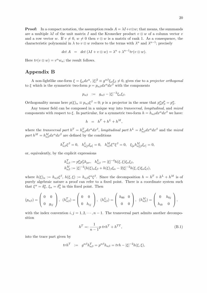
αξβ. Since the decomposition h = hT + hL + hM is ofpurely algebraic nature a proof can refer to a fixed point. There is a coordinate system suchthat ξα = δα0 , ξα = δ0α in this fixed point. Then

(pαβ) =

0 0

0 gij

, (hTαβ) =

0 0

0 hij

, (hLαβ) =

h00 0

0 0

, (hMαβ) =

0 h0j

hi0 0

,with the index convention i, j = 1, 2, · · · , n− 1. The transversal part admits another decompo-sition

hT =:1

n− 1p trhT + hTT , (B.1)

into the trace part given by

trhT := gαβhTαβ = pαβhαβ = trh− |ξ|−2h(ξ, ξ),

21

and the transversal-traceless part hTT which is just defined by (B.1). Notice that

hTTαβ ξα = 0, trhTT = 0.

An analogous decomposition formalism applies to plane waves

hαβ = aαβ exp (ikµxµ), aαβ = const, kµ = const, (B.2)

in a linear field theory for h = hαβdxαdxβ. The constant amplitudes aαβ form a symmetric

2-tensor a. In the case m2 ≡ |k|2 6= 0 the tensor a admits a unique decomposition into thetransversal, longitudinal, and mixed parts with respect to k: a = aT + aL + aM , such that incomponents

aTαβkβ = 0, aLα[βkµ] = 0, aMαβk

αkβ = 0, k[µaMα][βkν] = 0.

Two distinct informations are extracted from the transversal part aT : its trace traT := gαβaTαβand the transversal-traceless part of a

aTT := aT − 1

n− 1p traT ,

where the projection tensor p has the (constant) components pαβ = gαβ −m−2kαkβ.

A differential transformation h′ → h described by

h′αβ = hαβ −∇αvβ −∇βvα, (B.3)

turns, by the plane-wave ansatz

vα = ibα exp (ikµxµ),

into the algebraic transformation a′ → a described by

a′αβ = aαβ + kαbβ + kβbα (B.4)

which is also equivalent to

h′αβ = hαβ + kαvβ + kβvα. (B.5)

If the vacuum linearized gravitational theory is invariant under (B.3) then plane gravitationalwaves are transversal in the sense that the longitudinal and mixed parts aL, aM can be gaugedto zero as a consequence of the transversal gauge aαβk

β = 0, which can be achieved by atransformation (B.4).

Let us recall the particle content of the vacuum linearized Einstein’s equations δRαβ = 0,that is, the case κ > 0, a0 = a1 = a2 = 0: If m2 = |k|2 6= 0 then a plane-wave solution can begauged to zero by means of a transformation (B.4) or (B.5); hence, actually, there is no massiveparticle. If m2 = |k|2 = 0 then (B.2) solves δRαβ = 0 iff bαβk

β = 0, where

bαβ := aαβ −1

2gαβtra.

Notice that bαβkβ = 0 is a special case of the De Donder condition for solutions of δRαβ = 0

ψαβkβ = 0, ψαβ := hαβ −

1

2gαβtrh.

Vacuum Einstein gravity is homothetically invariant, that means, g → eφg, φ = const, impliesR′αβ = Rαβ. As a consequence, vacuum linearized Einstein gravity, described by δRαβ = 0, isinvariant under h′αβ = hαβ + λgαβ, λ = const. This kind of gauge transformations renderspossible a gauge condition tr h = 0. For plane waves, this is equivalent to tr a = 0. Thatmeans, there is no spin 0 particle. The massless particle in Einstein’s theory has spin 2.

22

References

[1] H. Weyl: Ann. Phys., IV. Folge, 59, 10, (1919) 101-133.

[2] A. S. Eddington: The Mathematical Theory of Relativity. Cammbridge University Press,1924.

[3] R. Schimming and H.-J. Schmidt: Gesch. Naturw., Techn., Med. Leipzig 27, (1990) 41-48.

[4] R. Schimming: Banach Center Publ., 12, (1984) 225-231.

[5] R. Schimming in: Proc. Internat. Seminar Math. Cosmology, Potsdam 1998. World Scien-tific, Singapore 1998, 39-46.

[6] R. Schimming: Cauchyproblem und Wellenlosungen der Bachschen Feldgleichungen derAllgemeinen Relativitatstheorie. Habilitationsschrift, Universitat Leipzig, 1979.

[7] R. Bach: Math. Zeitschrift, 9, (1921) 110-135.

[8] H. Buchdahl: J. Lond. Math. Soc., 26, (1951) 139-149.

[9] H. Buchdahl: J. Phys. A. Math. Gen., 12, 8, (1979) 1229-1234.

[10] H. Buchdahl: Acta Mathematica, 85, (1951) 63-72.

[11] H. Buchdahl: J. Phys. A, 12, 7, (1979) 1037-1043.

[12] H. Buchdahl: Quart. J. Math. Oxford, 19, 75, (1948) 150-159.

[13] C. Lanczos: Ann. Math., 39, (1958) 842-850.

[14] P. Havas: Gen. Rel. Grav., 8, 8, (1977) 631-645.

[15] H. Lee Chul and Hyun Kyu Lee: Mod. Phys. Lett. A, 3, 11, (1988) 1035-1039.

[16] H.-J. Schmidt: Ann. Phys., 7. Folge, 44, 5, (1987) 361-370.

[17] H.-J. Schmidt: Class. Quantum Grav., 7, (1990) 1023-1031.

[18] H.-J. Schmidt: Astro. Nachr., 307, 5, (1986) 339-340.

[19] K. Mobius: Feldfreiheitsgrade und Teilcheninhalt von Losungen der Gravitationsfeldgle-ichungen 4. Ordnung. Dissertation, Humboldt-Universitat Berlin, 1987.

[20] K. Mobius: Astron. Nachr., 309, 6, (1988) 357-362.

[21] P. Teyssandier: Astron. Nachr., 311,4, (1990) 209-212.

[22] P. Teyssandier and Ph. Tourrenc: J. Math. Phys., 24, 12, (1983) 2793-2799.

[23] N. H. Barth and S. M. Christensen: Phys. Rev. D, 28, 8, (1983) 1876-1893.

[24] H. Friedrich and A. D. Rendall: The Cauchy Problem for the Einstein Equations. Einstein’sField Equations and their Physical Interpretation (ed. B. G. Schmidt) Springer, Berlin,2000.

23

[25] E. Schmutzer: Relativistische Physik. Leipzig, 1968.

[26] P. K. Raschewski: Riemannsche Geometrie und Tensoranalysis. Veb Deutscher Verlag derWissenschaften, Berlin, 1959.

[27] M. Berger and D. Ebin: J. Diff. Geom., 3, (1969) 379-392.

[28] A. E. Fischer and J. E. Marsden: Canad. J. Math., 29, (1977) 193-209.

[29] N. O. Murchadha and J. W. York: Phys. Rev. D, 10, (1974) 428-436.

[30] N. O. Murchadha and J. W. York: Phys. Rev. D, 10, (1974) 437-446.

[31] P. Ehrenfest: Proc. Akad. Wet. Amsterdam 20, (1917) 200-209.