arX

iv:g

r-qc

/030

9112

v2 2

9 Se

p 20

03

Quasinormal modes of Schwarzschild black holes in four and higher dimensions

Vitor Cardoso,∗ Jose P. S. Lemos,† and Shijun Yoshida‡

Centro Multidisciplinar de Astrofısica - CENTRA,

Departamento de Fısica, Instituto Superior Tecnico,

Av. Rovisco Pais 1, 1049-001 Lisboa, Portugal,

(Dated: February 4, 2008)

We make a thorough investigation of the asymptotic quasinormal modes of the four and five-dimensional Schwarzschild black hole for scalar, electromagnetic and gravitational perturbations.Our numerical results give full support to all the analytical predictions by Motl and Neitzke, forthe leading term. We also compute the first order corrections analytically, by extending to higherdimensions, previous work of Musiri and Siopsis, and find excellent agreement with the numericalresults. For generic spacetime dimension number D the first-order corrections go as 1

n(D−3)/(D−2) .This means that there is a more rapid convergence to the asymptotic value for the five dimensionalcase than for the four dimensional case, as we also show numerically.

PACS numbers:

I. INTRODUCTION

The study of quasinormal modes of black holes beganmore than thirty years ago, when Vishveshwara [1] no-ticed that the signal from a perturbed black hole is, formost of the time, an exponentially decaying ringing sig-nal. It turns out that the ringing frequency and dampingtimescale are characteristic of the black hole, dependingonly on its parameters (like the mass and angular mo-mentum). We call these characteristic oscillations thequasinormal modes (QNMs) and the associated frequen-cies are termed quasinormal frequencies (QN frequen-cies), because they are really not stationary perturba-tions. Not surprisingly, QNMs play an important role inthe dynamics of black holes, and consequently in grav-itational wave physics. In fact, it is possible [2, 3] toextract the parameters of the black hole simply by ob-serving these QN frequencies, using for example gravita-tional wave detectors. The discovery that QNMs dom-inate the answer of a black hole to almost any exteriorperturbation was followed by a great effort to find, nu-merically and analytically, the QN frequencies. For ex-cellent reviews on the status of QNMs, prior to 2000, werefer the reader to Kokkotas and Schmidt [4] and Nollert[5]. It is important to note that on the astrophysical as-pect, the most important QN frequencies are the lowestones, i.e., frequencies with smaller imaginary part, andthe most important spacetimes are the asymptoticallyflat and perhaps now the asymptotically de Sitter. How-ever, three years ago Horowitz and Hubeny [6] pointedout that QNMs of black holes in anti-de Sitter space havea different importance. According to the AdS/CFT cor-respondence [7], a black hole in anti-de Sitter space may

∗Electronic address: vcardoso@fisica.ist.utl.pt†Electronic address: lemos@kelvin.ist.utl.pt‡Electronic address: yoshida@fisica.ist.utl.pt

be viewed as a thermal state in the dual theory. Perturb-ing this black hole corresponds to perturbing the thermalstate, and therefore the typical timescale of approach tothermal equilibrium (which is hard to compute directlyin the dual theory) should as well be governed by thelowest QN frequencies. That this is indeed the case wasproved by Birmigham, Sachs and Solodukhin [8] for theBTZ black hole, taking advantage that this is one of thefew spacetimes where one can compute exactly its QNfrequencies, as showed by Cardoso and Lemos [9]. Asimilar study was made by Kurita and Sakagami [10] forthe D-3 brane. This interpretation for the imaginary partof the QN frequencies in terms of timescales of approachto thermal equilibrium in the dual conformal field theoryhas motivated a generalized search for the quasinormalmodes of different black holes in anti-de Sitter spacetime,over the last three years [6, 9, 11].

Recently, the motivation for studying QN modes ofblack holes has grown enormously with the conjectures[12, 13, 14, 16] relating the highly damped QNMs (i.e.,QN frequencies with large imaginary parts) to black holearea quantization and to the Barbero Immirzi parameterappearing in Loop Quantum Gravity. The seeds of thatidea were planted some time ago by Bekenstein [17]. Asemi-classical reasoning of the conjecture [18, 19] that theblack hole area spectrum is quantized leads to

An = γ l2P n , n = 1, 2, ... . (1)

Here lP is the Planck length and γ is an undeterminedconstant. However, statistical physics arguments imposea constraint on γ [18, 20]:

γ = 4 log k , (2)

where k is an integer. The integer k was left undeter-mined (although there were some suggestions for it [19]),until Hod [12], supported by some of Bekenstein’s ideas,put forward the proposal to determine k via a versionof Bohr’s correspondence principle, in which one admits

2

that the real part of QN frequencies with a large imagi-nary part plays a fundamental role. It was seen numeri-cally by Nollert [5, 21] that QN frequencies with a largeimaginary part behave, in the Schwarzschild geometry as

ωM = 0.0437123 +i

8(2n + 1) , (3)

where M is the black hole mass, and n the mode number.Hod first realized that 0.0437123 ∼ ln 3

8π , and went on tosay that, if one supposes that the emission of a quantumwith frequency ln 3

8π corresponds to the least possible en-ergy a black hole can emit, then the change in surfacearea will be (using A = 16πM2)

∆A = 32πMdM = 32πM~ω = 4~ ln 3 . (4)

Comparing with (1) we then get k = 3 and therefore thearea spectrum is fixed to

An = 4 ln 3l2P n ; n = 1, 2, ... (5)

It was certainly a daring proposal to map 0.0437123 toln 3, and even more to use the QN frequencies to quan-tize the black hole area, by appealing to “Bohr’s corre-spondence principle”. The risk paid off: recently, Dreyer[13] put forward the hypothesis that if one uses such acorrespondence it is possible to fix a formerly free param-eter, the Barbero-Immirzi parameter, appearing in LoopQuantum Gravity. Dreyer’s work implied that the en-tropy has contributions from J = 1 edges mainly. Oneinterpretation (proposed by Dreyer), is that one changesthe gauge group from SU(2), which is the most naturalone, to SO(3). There are other explanations, though.For example, Corichi [15] presents an argument based onsimple conservation principles to suggest that one cankeep SU(2) and still have consistency with QNM, whileLing and Zhang [16] propose to consider the supersym-metric extension of the theory.

All of these proposals and conjectures could be uselessif one could not prove that the real part of the QN fre-quencies do approach ln 3

8π , i.e., that the number 0.0437123

in Nollert’s paper was exactly ln 38π . This was accom-

plished by Motl [22] some months ago, using an ingenioustechnique, working with the continued fraction represen-tation of the wave equation. Subsequently, Motl andNeitzke [23] used a more flexible and powerful approach,called the monodromy method, and were not only ableto rederive the four dimensional Schwarzschild value ln 3

8π ,but also to compute the asymptotic value for generic D-dimensional Schwarzschild black holes thereby confirm-ing a previous conjecture by Kunstatter [24]. They havealso predicted the form of the asymptotic QN frequenciesfor the Reissner-Nordstrom geometry, a prediction whichwas verified by Berti and Kokkotas [25].

It is interesting to speculate why, in thirty years inves-tigating QNMs and QN frequencies, no one has ever beenable to deduce analytically the asymptotic value of theQN frequencies, nor even for the Schwarzschild geometry,which is the simplest case. In our opinion, there are three

important facts that may help explain this: first, the con-cern was mostly with the lowest QN frequencies, the oneswith smaller imaginary part, since they are the most im-portant in the astrophysical context where QNMs wereinserted until three years ago. In fact, most of the tech-niques to find QN frequencies, and there were many, havebeen devised to compute the lowest QN frequencies (see[4, 5] for a review). Secondly, there was no suggestion forthe asymptotic ln 3 value. To know this value serves asa strong stimulation. The third reason is obvious: thiswas a very difficult technical problem.

It is thus satisfying that Motl and Neitzke have provedexactly that the limit is ln 3. In addition, Van den Brink[26] used a somewhat different approach to rederive theln 38π value, and at the same time computed the first or-der correction to gravitational QN frequencies, confirm-ing analytically Nollert’s [21] numerical results. However,Motl and Neitzke’s monodromy method is more flexibleand powerful: it has been easily adapted to other space-times. For example, Castello-Branco and Abdalla [27]have generalized the results to the Schwarzschild-de Sit-ter geometry, while Schiappa, Natario and Cardoso [28]have used it to compute the asymptotic values in theD-dimensional Reissner-Nordstrom geometry. Moreoverthe first order corrections are also easily obtained, as hasbeen showed by Musiri and Siopsis [29] for the four di-mensional Schwarzschild geometry. Here we shall alsogeneralize these first order corrections so that they canencompass a general D-dimensional Schwarzschild blackhole. A body of work has been growing on the subjectof computing highly damped QNMs, both in asymptot-ically flat and in de Sitter or anti-de Sitter spacetimes[30, 31].

As an aside, we note that one of the most intrigu-ing features of Motl and Neitzke’s technique is that theregion beyond the event horizon, which never enters inthe definition of quasinormal modes, plays an extremelyimportant role. In particular, the singularity at r = 0is decisive for the computation. At the singularity theeffective potential for wave propagation blows up. Some-how, the equation, or the singularity, knows what we areseeking! It is also worth of note the following: for highfrequencies, or at least frequencies with a large imaginarypart, the important region is therefore r = 0 where thepotential blows up, whereas for low frequencies, of inter-est for late-time tails [32], it is the other limit, r → ∞which is important.

The purpose of this paper is two-fold: first we wantto enlarge and settle the results for the four dimensionalSchwarzschild black hole. We shall first numerically con-firm Nollert’s results for the gravitational case, and Bertiand Kokkotas’[25] results for the scalar case, and see thatthe match between these and the analytical prediction isquite good. Then we shall fill-in a gap left behind in thesetwo studies: the electromagnetic asymptotic QN frequen-cies, for which there are no numerical results, but a lotof analytical predictions. This will put the monodromymethod on a firmer ground. One might say that in the

3

present context (of black hole quantization and relationwith Loop Quantum Gravity) electromagnetic perturba-tions are not relevant, only the gravitational ones are.This is not true though, because when considering theReissner-Nordstrom case gravitational and electromag-netic perturbations are coupled [33] and it is thereforeof great theoretical interest to study each one separately,in the case they do decouple, i.e., the Schwarzschild ge-ometry. We find that all the analytical predictions arecorrect: scalar and gravitational QN frequencies asymp-tote to ω

TH= ln 3+i(2n+1)π with 1√

ncorrections, where

TH = 18πM is the Hawking temperature. The corrections

are well described by the existing analytical formulas. Onthe other hand, electromagnetic QN frequencies asymp-tote to ω

TH= 0 + i2nπ with no 1√

ncorrections, as pre-

dicted by Musiri and Siopsis [29]. Indeed we find thatthe corrections seem to appear only at the 1

n3/2 level.The second aim of this paper is to establish numer-

ically the validity of the monodromy method by ex-tending the numerical calculation to higher dimensionalSchwarzschild black holes, in particular to the five dimen-sional one. We obtain numerically in the five dimensionalcase the asymptotic value of the QN frequencies, whichturns out to be ln 3+i(2n+1)π (in units of the black holetemperature), for scalar, gravitational tensor and gravi-tational vector perturbations. Equally important, is thatthe first order corrections appear as 1

n2/3 for these cases.We shall generalize Musiri and Siopsis’ method to higherdimensions and find that (i) the agreement with the nu-merical data is very good (ii) In generic D dimensionsthe corrections appear at the 1

n(D−3)/(D−2) level. Elec-tromagnetic perturbations in five dimensions seem to bespecial: according to the analytical prediction by Motland Neitzke, they should not have any asymptotic QNfrequencies. Our numerics seem not to go higher enoughin mode number to prove or disprove this. They indicatethat the real part approaches zero, as the mode numberincreases, but we have not been able to follow the QNfrequencies for very high overtone number. We also givecomplete tables for the lowest lying QN frequencies ofthe five dimensional black holes, and confirm previous re-sults [34, 35, 36, 37] for the fundamental QN frequenciesobtained using WKB-like methods. We find no purelyimaginary QN frequencies for the gravitational QNMs,which may be related to the fact that the potentials areno longer superpartners.

II. QN FREQUENCIES OF THE

FOUR-DIMENSIONAL SCHWARZSCHILD

BLACK HOLE

The first computation of QN frequencies of four-dimensional Schwarzschild black holes was carried outby Chandrasekhar and Detweiler [38]. They were onlyable to compute the lowest lying modes, as it was andstill is quite hard to find numerically QN frequencieswith a very large imaginary part. After this pioneer-

ing work, a number of analytical, semi-analytical andnumerical techniques were devised with the purpose ofcomputing higher order QNMs and to establish the low-lying ones using different methods [4, 5]. The most suc-cessful numerical method to study QNMs of black holeswas proposed by Leaver [39]. In a few words his methodamounts to reducing the problem to a continued frac-tion, rather easy to implement numerically. Using thismethod Leaver was able to determine the first 60 modesof the Schwarzschild black hole, which at that time wasabout an order of magnitude better than anyone had evergone before. The values of the QN frequencies he deter-mined, and we note he only computed gravitational ones,suggested that there is an infinite number of QN modes,that the real part of the QN frequencies approach a finitevalue, while the imaginary part grows without bound.That the real part of the QN frequencies approach a finitevalue was however opened to debate [40]: it seemed onestill had to go higher in mode number in order to ascer-tain the true asymptotic behaviour. Nollert [21] showeda way out of these problems: he was able to improveLeaver’s method in a very simple fashion so as to go verymuch higher in mode number: he was able to computemore than 2000 modes of the gravitational QNMs. Hisresults were clear: the real part of the gravitational QNfrequencies approaches a constant value ∼ 0.0437123/M ,and this value is independent of l. The imaginary partgrows without bound as (2n + 1)/8 where n is any largeinteger. These asymptotic behaviours have both leadingcorrections, which were also determined by Nollert. Hefound that to leading order the asymptotic behaviour ofthe gravitational QN frequencies of a Schwarzschild blackhole is given by Eq. (3) plus a leading correction, namely,

ωM = 0.0437123 +i

8(2n + 1) +

a√n

, (6)

where the correction term a depends on l. About tenyears later, Motl [22] proved analytically that this is in-deed the correct asymptotic behaviour. To be precise heproved that

ω

TH= ln 3 + i (2n + 1)π + corrections . (7)

Since the Hawking temperature TH is TH = 18πM ,

Nollert’s result follows. He also proved that this same re-sult also holds for scalar QN frequencies, whereas electro-magnetic QN frequencies asymptote to a zero real part.Motl and Neitzke [23] using a completely different ap-proach, have rederived this result whereas Van den Brink[26] was able to find the leading asymptotic correctionterm a in (6) for the gravitational case. Very recently,Musiri and Siopsis [29], leaning on Motl and Neitzke’stechnique, have found the leading correction term for anyfield, scalar, electromagnetic and gravitational. This cor-rection term is presented in section III B, where we alsogeneralize to higher dimensional black holes. In particu-lar, for electromagnetic perturbations they find that thefirst order corrections are zero.

4

FIG. 1: Scalar (s = 0), electromagnetic (s = 1) andgravitational (s = 2) QN frequencies of a four-dimensionalSchwarzschild black hole. Note that the dots indicate the QNfrequencies there, and the lines connecting the dots only helpto figure out to which multipole (l, s) they belong to. We showthe lowest 500 modes for the lowest radiatable multipoles ofeach field, i.e., l = 0 for the scalar field, l = 1 for the electro-magnetic and l = 2 for gravitational. However, the asymp-totic behaviour is l-independent. It is quite clear from thisplot that highly damped electromagnetic QN frequencies havea completely different behaviour from that of scalar or gravita-tional highly damped QN frequencies. In fact, the electromag-netic ones asymptote to ω

TH→ i(2n)π , n → ∞, as predicted

by Motl [22] and Motl and Neitzke [23]. The scalar and grav-itational ones asymptote to ω

TH→ ln 3 + i(2n + 1)π , n → ∞.

Here we use Nollert’s method to compute scalar, elec-tromagnetic and gravitational QN frequencies of the four-dimensional Schwarzschild black hole. The details on theimplementation of this method in four dimensions arewell known and we shall not dwell on it here any more.We refer the reader to the original references [21, 39].

Our results are summarized in Figures 1-2, and TablesI- II. In Fig. 1 we show the behaviour of the 500 low-est QN frequencies for the lowest radiatable multipole ofeach field (we actually have computed the first 5000 QNfrequencies, but for a better visualization we do not showthem all): l = 0 for scalar, l = 1 for electromagnetic andl = 2 gravitational. Note that in Fig. 1, as well as inall other plots in this work, the dots indicate the QNfrequencies there, and the lines connecting the dots onlyhelp to figure out to which multipole (l, s) they belongto. In what concerns the asymptotic behaviour, our nu-merics show it is not dependent on l, and that formula(6) holds. The results for the scalar and gravitational QNfrequencies are not new: the gravitational ones have beenobtained by Nollert [21], as we previously remarked, andthe scalar ones have been recently arrived at by Berti andKokkotas [25]. Here we have verified both. Both scalarand gravitational QN frequencies have a real part asymp-

TABLE I: The correction coefficients for the four-dimensionalSchwarzschild black hole, both numerical, here labeled as“CorrN4 ” and analytical, labeled as “CorrA4 ”. These resultsrefer to scalar perturbations. The analytical results are ex-tracted from [29] (see also formula (29 below). Notice thevery good agreement between the numerically extracted re-sults and the analytical prediction.These values were obtainedusing the first 5000 modes.

s = 0

l CorrN4 : CorrA4

0 1.20-1.20i 1.2190-1.2190i

1 8.52- 8.52i 8.5332-8.5332i

2 23.15-23.15i 23.1614-23.1614i

3 44.99-44.99i 45.1039-45.1039i

4 74.34-74.34i 74.3604-74.3605i

toting to ln 3 × TH . Electromagnetic QN frequencies, onthe other hand, have a real part asymptoting to 0. Thisis clearly seen in Fig. 1. For gravitational perturbationsNollert found, and we confirm, that the correction terma in (6) is

a = 0.4850 , l = 2

a = 1.067 , l = 3 (8)

We have also computed the correction terms for the scalarcase, and we have obtained results in agreement withBerti and Kokkotas’ ones [25] . Our results are summa-rized in Tables I-II, where we also show the analyticalprediction [29] (see section III B). To fix the conventionsadopted throughout the rest of the paper, we write

ω

TH= ln 3 + i(2n + 1)π +

Corr√n

. (9)

Thus, the correction term a in (6) is related to Corr bya = Corr × TH .

As for the electromagnetic correction terms, we foundit was not very easy to determine them. In fact, it ishard, even using Nollert’s method, to go very high inmode number for these perturbations (we have made itto n = 5000). The reason is tied to the fact that thesefrequencies asymptote to zero, and it is hard to deter-mine QN frequencies with a vanishingly small real part.Nevertheless, there are some features one can be sure of.We have fitted the electromagnetic data to the followingform ω

TH= i(2n)π + b√

n, and found that this gave very

poor results. Thus one saw numerically that the first or-der correction term is absent, as predicted in [29] (see alsosection III B where we rederive these corrections, gener-alizing them to arbitrary dimension). Our data seems toindicate that the leading correction term is of the form

bn3/2 . This is more clearly seen in Fig. 2 where we plotthe first electromagnetic QN frequencies on a ln plot.For frequencies with a large imaginary part, the slope is

5

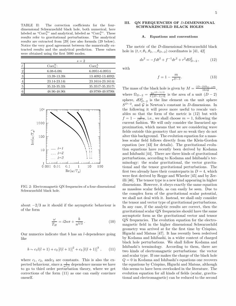
TABLE II: The correction coefficients for the four-dimensional Schwarzschild black hole, both numerical, herelabeled as “CorrN4 ” and analytical, labeled as “CorrA4 ”. Theseresults refer to gravitational perturbations. The analyticalresults are extracted from [29] (see also formula (29 below).Notice the very good agreement between the numerically ex-tracted results and the analytical prediction. These valueswere obtained using the first 5000 modes.

s = 2

l CorrN4 : CorrA4

2 6.08-6.08i 6.0951-6.0951i

3 13.39-13.39i 13.4092-13.4092i

4 23.14-23.14i 23.1614-23.1614i

5 35.33-35.33i 35.3517-35.3517i

6 48.90-48.90i 49.9799-49.9799i

FIG. 2: Electromagnetic QN frequencies of a four-dimensionalSchwarzschild black hole.

about −2/3 as it should if the asymptotic behaviour isof the form

ω

TH= i2nπ +

b

n3/2. (10)

Our numerics indicate that b has an l-dependence goinglike

b ∼ c1l(l + 1) + c2 [l(l + 1)]2+ c3 [l(l + 1)]

3, (11)

where c1, c2, andc3 are constants. This is also the ex-pected behaviour, since a 1

n3/2 dependence means we haveto go to third order perturbation theory, where we getcorrections of the form (11) as one can easily convinceoneself.

III. QN FREQUENCIES OF D-DIMENSIONAL

SCHWARZSCHILD BLACK HOLES

A. Equations and conventions

The metric of the D-dimensional Schwarzschild blackhole in (t, r, θ1, θ2, .., θD−2) coordinates is [41, 42]

ds2 = −fdt2 + f−1dr2 + r2dΩ2D−2 , (12)

with

f = 1 − m

rD−3. (13)

The mass of the black hole is given by M = (D−2)ΩD−2m16πG ,

where ΩD−2 = 2π(D−1)/2

Γ[(D−1)/2] is the area of a unit (D − 2)

sphere, dΩ2D−2 is the line element on the unit sphere

SD−2, and G is Newton’s constant in D-dimensions. Inthe following it will prove more useful to rescale vari-ables so that the form of the metric is (12) but withf = 1 − 1

rD−3 , i.e., we shall choose m = 1, following thecurrent fashion. We will only consider the linearized ap-proximation, which means that we are considering wavefields outside this geometry that are so weak they do notalter this background. The evolution equation for a mass-less scalar field follows directly from the Klein-Gordonequation (see [43] for details). The gravitational evolu-tion equations have recently been derived by Kodamaand Ishibashi [44]. There are three kinds of gravitationalperturbations, according to Kodama and Ishibashi’s ter-minology: the scalar gravitational, the vector gravita-tional and the tensor gravitational perturbations. Thefirst two already have their counterparts in D = 4, whichwere first derived by Regge and Wheeler [45] and by Zer-illi [46]. The tensor type is a new kind appearing in higherdimensions. However, it obeys exactly the same equationas massless scalar fields, as can easily be seen. Due tothe complex form of the gravitational scalar potential,we shall not deal with it. Instead, we shall only considerthe tensor and vector type of gravitational perturbations.In any case, if the analytic results are correct, then thegravitational scalar QN frequencies should have the sameasymptotic form as the gravitational vector and tensorQN frequencies. The evolution equation for the electro-magnetic field in the higher dimensional Schwarzschildgeometry was arrived at for the first time by Crispino,Higuchi and Matsas [47]. It has recently been rederivedby Kodama and Ishibashi, in a wider context of chargedblack hole perturbations. We shall follow Kodama andIshibashi’s terminology. According to them, there aretwo kinds of electromagnetic perturbations: the vectorand scalar type. If one makes the charge of the black holeQ = 0 in Kodama and Ishibashi’s equations one recoversthe equations by Crispino, Higuchi and Matsas, althoughthis seems to have been overlooked in the literature. Theevolution equation for all kinds of fields (scalar, gravita-tional and electromagnetic) can be reduced to the second

6

order differential equation

d2Ψ

dr2∗

+ (ω2 − V )Ψ = 0 , (14)

where r is a function of the tortoise coordinate r∗, definedthrough ∂r

∂r∗

= f(r), and the potential can be written incompact form as

V = f(r)

[

l(l + D − 3)

r2+

(D − 2)(D − 4)

4r2+

(1 − j2)(D − 2)2

4rD−1

]

. (15)

The constant j depends on what kind of field one is study-ing:

j =

0 , scalar and gravitational tensor

perturbations.

1 , gravitational vector

perturbations.2

D−2 , electromagnetic vector

perturbations.

2 − 2D−2 , electromagnetic scalar

perturbations .

(16)

Notice that in four dimensions, j reduces to the usual val-ues given by Motl and Neitzke [23]. According to our con-ventions, the Hawking temperature of a D-dimensionalSchwarzschild black hole is

TH =D − 3

4π(17)

Our purpose here is to investigate the QN frequenciesof higher dimensional black holes. Of course one cannotstudy every D. We shall therefore focus on one particu-lar dimension, five, and make a complete analysis of itsQN frequencies. The results should be representative.In particular, one feature that distinguishes an arbitraryD from the four dimensional case is that the correctionterms come with a different power, i.e., whereas in fourdimensions the correction is of the form 1√

nwe shall find

that in generic D it is of the form 1n(D−3)/(D−2) . Thus, if

one verifies this for D = 5 for example, one can ascertainit will hold for arbitrary D. We shall now briefly sketchour numerical procedure for finding QN frequencies ofa five dimensional black hole. This is just Leaver’s andNollert’s technique with minor modifications.

The QNMs of the higher-dimensional Schwarzschildblack hole are characterized by the boundary conditionsof incoming waves at the black hole horizon and outgoingwaves at spatial infinity, written as

Ψ(r) →

e−iωr∗ as r∗ → ∞eiωr∗ as r∗ → −∞ ,

(18)

where the time dependence of perturbations has beenassumed to be eiωt.

B. Perturbative calculation of QNMs of

D-dimensional Schwarzschild black holes

In this section we shall outline the procedure for com-puting the first order corrections to the asymptotic valueof the QN frequencies of a D-dimensional Schwarzschildblack hole. This will be a generalization of Musiri andSiopsis’ method [29], so we adopt all of their notation,and we refer the reader to their paper for further details.The computations are however rather tedious and the fi-nal expressions are too cumbersome, so we shall refrainfrom giving explicit expressions for the final result.

We start with the expansion of the potential V nearthe singularity r = 0. One can easily show that near thispoint the potential (15) may be approximated as

V ∼ − ω2

4z2

[

1 − j2 +A

(−zω)(D−3)/(D−2)

]

, (19)

where we adopted the conventions in [29] and thereforez = ωr∗. The constant A is given by

A =4l(l + D − 3) + (D − 2)(D − 4) − (D − 2)2(1 − j2)

(D − 2)(D−1)/(D−2)+

2(1 − j2)(D − 2)(2D−5)/(D−2)

2D − 5. (20)

In D = 4 this reduces to the usual expression [29, 48]for the potential near r = 0. Expression (19) is a formalexpansion in 1

ω(D−3)/(D−2) , so we may anticipate that in-deed the first order corrections will appear in the form

1n(D−3)/(D−2) . So now we may proceed in a direct manner:

we expand the wavefunction to first order in 1ω(D−3)/(D−2)

as

Ψ = Ψ(0) +1

ω(D−3)/(D−2)Ψ(1) , (21)

and find that the first-order correction obeys the equation

d2Ψ(1)

dz2+(

1 − j2

4z2+1)Ψ(1) = ω(D−3)/(D−2)δV Ψ(0) , (22)

with

δV = − A

ω(D−3)/(D−2)(−z)(D−1)/(D−2). (23)

All of Musiri and Siopsis’ expressions follow directly tothe D-dimensional case, if one makes the replacement√−ωr0 → ω(D−3)/(D−2) in all their expressions. For ex-

ample, the generalsolution of (22) is

Ψ(1)± = CΨ

(0)+

∫ z

0

Ψ(0)− δV Ψ

(0)± − CΨ

(0)−

∫ z

0

Ψ(0)+ δV Ψ

(0)± ,

(24)where

C =ω(D−3)/(D−2)

sin jπ/2, (25)

7

and the wavefunctions Ψ(0)± are

Ψ(0)± =

√

πz

2J±j/2(z) . (26)

The only minor modification is their formula (30). InD-dimensions, it follows that

Ψ(1)± = z1±j/2+kG±(z) , (27)

where k = D−42(D−2) , and G± are even analytic functions

of z. So we have all the ingredients to construct the firstorder corrections in the D-dimensional Schwarzschild ge-ometry. Unfortunately the final expressions turn out tobe quite cumbersome, and we have not managed to sim-plify them. We have worked with the symbolic manip-ulator Mathematica. It is possible to obtain simple ex-pression for any particular D, but apparently not for ageneric D. For generic D we write

ω

TH= ln (1 + 2 cosπj)+i(2n+1)π+

CorrDω(D−3)/(D−2)

(28)

So the leading term is ωTH

= ln 3 + i(2n + 1)π, for scalar,gravitational tensor and gravitational tensor perturba-tions (and the same holds for gravitational scalar). How-ever, for electromagnetic perturbations (vector or scalar)in D = 5, 1 + 2 cosπj = 1 + 2 cos 2π

3 = 0. So there seemto be no QN frequencies as argued by Motl and Neitzke[23]. We obtained for D = 4 the following result for thecorrection coefficient in (28),

Corr4 = −(1 − i)π3/2(−1 + j2 − 3l(l + 1)) cos jπ

2 Γ[1/4]

3(1 + 2 cos jπ)Γ[3/4]Γ[3/4− j/2]Γ[3/4 + j/2],

(29)which reduces to Musiri and Siopsis’ expression. For D =5 it is possible also to find a simple expression for thecorrections:

Corr5 =i(9j2 − (24 + 20l(l + 2)))π3/2

120 × 31/3Γ[2/3]Γ[2/3− j/2]Γ[2/3 + j/2]

×Γ[1/6]

eijπ

sin ((1/3+j/2)π) −1

sin ((2/3+j/2)π)

−1 + eijπ. (30)

The limits j → 0, 2 are well defined and yield

Corr5j=0 =

(1 − i√

3)(6 + 10l + 5l2)π3/2Γ[1/6]

45 × 31/3Γ[2/3]3, (31)

Corr5j=2 =

(−1 + i√

3)(−3 + 10l + 5l2)π3/2Γ[1/6]

45 × 31/3Γ[−1/3]Γ[2/3]Γ[5/3],

(32)We list in Tables VI-VII some values of this five dimen-sional correction for some values of the parameter j and land compare them with the results extracted numerically.The agreement is quite good. The code for extracting thegeneric D-dimensional corrections is available from theauthors upon request. It should not come as a surprisethat for j = 2/3 the correction term blows up: indeedalready the zeroth order term is not well defined.

C. Numerical procedure and results

1. Numerical procedure

In order to numerically obtain the QN frequencies,in the present investigation, we make use of Nollert’smethod [5], since asymptotic behaviors of QNMs in thelimit of large imaginary frequencies are prime concern inthe present study.

In our numerical study, we only consider the QNMsof the Schwarzschild black hole in the five dimensionalspacetime, namely the D = 5 case. As we have remarked,this should be representative. The tortoise coordinate isthen reduced to

r∗ = x−1 +1

2x1ln(x − x1) −

1

2x1ln(x + x1) , (33)

where x = r−1 and x1 = r−1h . Here, rh stands for the

horizon radius of the black hole. The perturbation func-tion Ψ may be expanded around the horizon as

Ψ = e−iωx−1

(x−x1)ρ(x+x1)

ρ∞∑

k=0

ak

(

x − x1

−x1

)k

, (34)

where ρ = iω/2x1 and a0 is taken to be a0 = 1. Theexpansion coefficients ak in equation (34) are determinedvia the four-term recurrence relation (it’s just a matter ofsubstituting expression (34) in the wave equation (14)),given by

α0a1 + β0a0 = 0 ,

α1a2 + β1a1 + γ1a0 = 0 , (35)

αkak+1 + βkak + γkak−1 + δkak−2 = 0 , k = 2, 3, · · · ,

where

αk = 2(2ρ + k + 1)(k + 1) ,

βk = −5(2ρ + k)(2ρ + k + 1) − l(l + 2) − 3

4

−9

4(1 − j2) ,

γk = 4(2ρ + k − 1)(2ρ + k + 1) +9

2(1 − j2) ,

δk = −(2ρ + k − 2)(2ρ + k + 1) − 9

4(1 − j2) .

It is seen that since the asymptotic form of the pertur-bations as r∗ → ∞ is written in terms of the variable xas

e−iωr∗ = e−iωx−1

(x − x1)−ρ(x + x1)

ρ , (36)

the expanded perturbation function Ψ defined by equa-tion (34) automatically satisfy the QNM boundary con-ditions (18) if the power series converges for 0 ≤ x ≤ x1.Making use of a Gaussian elimination [49], we can reduce

8

the four-term recurrence relation to the three-term one,given by

α′0a1 + β′

0a0 = 0 ,

α′kak+1 + β′

kak + γ′kak−1 = 0 , k = 1, 2, · · · , (37)

where α′k, β′

k, and γ′k are given in terms of αk, βk, γk and

δk by

α′k = αk, β′

k = βk, γ′k = γk, for k = 0, 1, (38)

and

α′k = αk,

β′k = βk − α′

k−1δk/γ′k−1 , (39)

γ′k = γk − β′

k−1δk/γ′k−1 , for k ≥ 2 .

Now that we have the three-term recurrence relation fordetermining the expansion coefficients ak, the conver-gence condition for the expansion (34), namely the QNMconditions, can be written in terms of the continued frac-tion as [39, 50]

β′0 −

α′0γ

′1

β′1−

α′1γ

′2

β′2−

α′2γ

′3

β′3−

... ≡ β′0 −

α′0γ

′1

β′1 −

α′

1γ′

2

β′

2−α′

2γ′

3β′

3−...

= 0 ,(40)

where the first equality is a notational definition com-monly used in the literature for infinite continued frac-tions. Here we shall adopt such a convention. In orderto use Nollert’s method, with which relatively high-orderQNM with large imaginary frequencies can be obtained,we have to know the asymptotic behaviors of ak+1/ak inthe limit of k → ∞. According to a similar considerationas that by Leaver [49], it is found that

ak+1

ak= 1 ± 2

√ρ k−1/2 +

(

2ρ − 3

4

)

k−1 + · · · , (41)

where the sign for the second term in the right-hand sideis chosen so as to be

Re(±2√

ρ) < 0 . (42)

In actual numerical computations, it is convenient tosolve the k-th inversion of the continue fraction equation(40), given by

β′k −

α′k−1γ

′k

β′k−1−

α′k−2γ

′k−1

β′k−2−

· · · α′0γ

′1

β′0

=α′

kγ′k+1

β′k+1−

α′k+1γ

′k+2

β′k+2−

· · · . (43)

The asymptotic form (41) plays an important role inNollert’s method when the infinite continued fraction inthe right-hand side of equation (43) is evaluated [5].

TABLE III: The first lowest QN frequencies for scalar andgravitational tensor (j = 0) perturbations of the five dimen-sional Schwarzschild black hole. The frequencies are normal-ized in units of black hole temperature, so the Table reallyshows ω

TH, where TH is the Hawking temperature of the black

hole.

j = 0

n l = 0: l = 1: l = 2

0 3.3539+2.4089i 6.3837+2.2764i 9.4914+2.2462i

1 2.3367+8.3101i 5.3809+7.2734i 8.7506+6.9404i

2 1.8868+14.786i 4.1683+13.252i 7.5009+12.225i

3 1.6927+21.219i 3.4011+19.708i 6.2479+18.214i

4 1.5839+27.607i 2.9544+26.215i 5.3149+24.597i

2. Numerical results

Using the numerical technique described in sectionIII C 1 we have extracted the 5000 lowest lying QN fre-quencies for the five dimensional Schwarzschild blackhole, in the case of scalar, gravitational tensor and grav-itational vector perturbations. For electromagnetic vec-tor perturbations the situation is different: the real partrapidly approaches zero, and we have not been able tocompute more than the first 30 modes.

(i) Low-lying modes

Low lying modes are important since they govern theintermediate-time evolution of any black hole perturba-tion. As such they may play a role in TeV-scale gravityscenarios [51], and higher dimensional black hole forma-tion [34, 52]. For example, it is known [34, 53, 54] that ifone forms black holes through the high energy collisionof particles, then the fundamental quasinormal frequen-cies serve effectively as a cuttof in the energy spectra ofthe gravitational energy radiated away. In Tables III-Vwe list the five lowest lying QN frequencies for some val-ues of the multipole index l. The fundamental modesare in excellent agreement with the ones presented byKonoplya [35, 36] using a high-order WKB approach.Notice he uses a different convention so one has to becareful when comparing the results. For example, in ourunits Konoplya obtains for scalar and tensorial pertur-bations (j = 0) with l = 2 a fundamental QN frequencyω0/TH = 9.49089 + 2.24721i, whereas we get, from Ta-ble III the number 9.4914 + 2.2462i so the WKB ap-proach does indeed yield good results, at least for low-lying modes, since it is known it fails for high-order ones.

In the four dimensional case, and for gravitational vec-tor perturbations, there is for is each l, a purely imag-inary QN frequency, which had been coined an “alge-braically special frequency” by Chandrasekhar [33]. Forfurther properties of this special frequencies we refer thereader to [55]. The existence of these purely imagi-nary frequencies translates, in the four dimensional case,

9

TABLE IV: The first lowest QN frequencies for gravita-tional vector (j = 2) perturbations of the five dimensionalSchwarzschild black hole. The frequencies are normalized inunits of black hole temperature, so the Table really shows ω

TH,

where TH is the Hawking temperature of the black hole.

j = 2

n l = 2: l = 3: l = 4

0 7.1251+2.0579i 10.8408+2.0976i 14.3287+2.1364i

1 5.9528+6.4217i 8.8819+1.0929i 12.8506+1.0574i

2 3.4113+12.0929i 7.2160+16.3979i 11.5069+16.0274i

3 2.7375+19.6094i 5.5278+22.3321i 9.99894+21.5009i

4 2.5106+26.2625i 3.9426+28.6569i 8.56386+27.4339i

TABLE V: The first lowest QN frequencies for electromag-netic vector (j = 2/3) perturbations of the five dimensionalSchwarzschild black hole. The frequencies are normalized inunits of black hole temperature, so the Table really shows ω

TH,

where TH is the Hawking temperature of the black hole.

j = 2/3

n l = 1: l = 2: l = 3

0 5.9862+2.2038i 9.2271+2.2144i 12.4184+2.2177i

1 4.9360+7.0676i 8.4728+6.8459i 11.8412+6.7660i

2 3.6588+12.9581i 7.1966+12.0804i 10.7694+11.6626i

3 2.8362+19.3422i 5.9190+18.0343i 9.4316+17.1019i

4 2.3322+25.7861i 4.9682+24.3832i 8.1521+23.0769i

a relation between the two gravitational wavefunctions(i.e., between the Regge-Wheeler and the Zerilli wave-function, or between the gravitational vector and gravi-tational scalar wavefunctions, respectively). It is possi-ble to show for example that the associated potentialsare related through supersymmetry. Among other con-sequences, this relation allows one to prove that the QNfrequencies of both potentials are exactly the same [33].

We have not spotted any purely imaginary QN fre-quency for this five-dimensional black hole. In fact theQN frequency with the lowest real part is a gravitationalvector QN frequency with l = 4 and overtone numbern = 13, ω = 8.7560× 10−2 + 6.9934i. This may indicatethat in five dimensions, there is no relation between thewavefunctions, or put another way, that the potentialsare no longer superpartner potentials. This was in factalready observed by Kodama and Ishibashi [44] for anydimension greater than four. It translates also in TablesIII-IV, which yield different values for the QN frequen-cies. Although we have not worked out the gravitationalscalar QN frequencies, a WKB approach can be used forthe low-lying QN frequencies, and also yields differentvalues [35, 36].

(ii) Highly damped modes

Our numerical results for the highly damped modes,

FIG. 3: The QN frequencies of scalar (j = 0), gravitationalvector (j = 2) and electromagnetic vector (j = 2/3) pertur-bations of a five-dimensional Schwarzschild black hole. Weonly show the lowest radiatable multipoles, but the asymtp-toic behaviour is l-independent.

i.e., QN frequencies with a very large imaginary part,are summarized in Figures 3-5 and in Tables VI-VII.

In Fig. 3 we show our results for scalar, gravitationaltensor (j = 0), gravitational vector (j = 2) and electro-magnetic vector (j = 2/3) QN frequencies. For j = 0 , 2the real part approaches ln 3 in units of the black holetemperature, a result consistent with the analytical re-sult in [23] (see also section III B). Electromagnetic vec-tor (j = 2/3) QN frequencies behave differently: the realpart rapidly approaches zero, and this makes it very dif-ficult to compute the higher modes. In fact, the samekind of problem appears in the Kerr geometry [30], andthis a major obstacle to a definitive numerical charac-terization of the highly damped QNMs in this geometry.We have only been able to compute the first 30 modeswith accuracy. The prediction of [23] for this case (seesection III B) is that there are no asymptotic QN frequen-cies. It is left as an open question whether this is true ornot. Our results indicate that the real part rapidly ap-proaches zero, but we cannot say whether the modes diethere or not, or even if they perform some kind of oscil-lation. The imaginary part behaves in the usal manner,growing linearly with mode number.

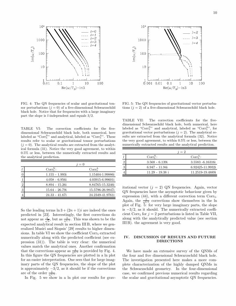
Let us now take a more detailed look at our numeri-cal data for scalar and gravitational QN frequencies. InFig. 4 we show in a ln plot our results for scalar andgravitational tensor (j = 0) QN frequencies.

Our numerical results are very clear: asymptoticallythe QN frequencies for scalar and gravitational tensorperturbations (j = 0) behave as

ω

TH= ln 3 + i (2n + 1)π +

Corr5n2/3

, (44)

10

FIG. 4: The QN frequencies of scalar and gravitational ten-sor perturbations (j = 0) of a five-dimensional Schwarzschildblack hole. Notice that for frequencies with a large imaginarypart the slope is l-independent and equals 3/2.

TABLE VI: The correction coefficients for the five-dimensional Schwarzschild black hole, both numerical, herelabeled as “CorrN5 ” and analytical, labeled as “CorrA5 ”. Theseresults refer to scalar or gravitational tensor perturbations(j = 0). The analytical results are extracted from the analyt-ical formula (31). Notice the very good agreement, to within0.5% or less, between the numerically extracted results andthe analytical prediction.

j = 0

l CorrN5 : CorrA5

0 1.155 - 1.993i 1.15404-1.99886i

1 4.058 - 6.956i 4.03915-6.99601i

2 8.894 - 15.26i 8.84765-15.3246i

3 15.64 - 26.79i 15.5796-26.9847i

4 24.33 - 41.67i 24.2349-41.9761i

So the leading terms ln 3 + (2n + 1)i are indeed the onespredicted in [23]. Interestingly, the first corrections donot appear as 1√

n, but as 1

n2/3 . This was shown to be the

expected analytical result in section III B, where we gen-eralized Musiri and Siopsis’ [29] results to higher dimen-sions. In table VI we show the coefficient Corr5 extractednumerically along with the predicted coefficient (see ex-pression (31)). The table is very clear: the numericalvalues match the analytical ones. Another confirmationthat the corrections appear as 1

n2/3 is provided by Fig. 4.In this figure the QN frequencies are plotted in a ln plotfor an easier interpretation. One sees that for large imag-inary parts of the QN frequencies, the slope of the plotis approximately −3/2, as it should be if the correctionsare of the order 1

n2/3 .In Fig. 5 we show in a ln plot our results for grav-

FIG. 5: The QN frequencies of gravitational vector perturba-tions (j = 2) of a five-dimensional Schwarzschild black hole.

TABLE VII: The correction coefficients for the five-dimensional Schwarzschild black hole, both numerical, herelabeled as “CorrN5 ” and analytical, labeled as “CorrA5 ”, forgravitational vector perturbations (j = 2). The analytical re-sults are extracted from the analytical formula (32). Noticethe very good agreement, to within 0.5% or less, between thenumerically extracted results and the analytical prediction.

j = 2

l CorrN5 : CorrA5 :

2 3.568 - 6.139i 3.5583 -6.16316i

3 6.947 - 11.94i 6.92425-11.9932i

4 11.29 - 19.38 i 11.2519-19.4889i

itational vector (j = 2) QN frequencies. Again, vectorQN frequencies have the asymptotic behaviour given byexpression (44), with a different correction term Corr5.Again, the 1

n2/3 corrections show themselves in the lnplot of Fig. 5: for very large imaginary parts, the slopeis −3/2, as it should. The numerically extracted coeffi-cient Corr5 for j = 2 perturbations is listed in Table VII,along with the analytically predicted value (see sectionIII B). the agreement is very good.

IV. DISCUSSION OF RESULTS AND FUTURE

DIRECTIONS

We have made an extensive survey of the QNMs ofthe four and five dimensional Schwarzschild black hole.The investigation presented here makes a more com-plete characterization of the highly damped QNMs inthe Schwarzschild geometry. In the four-dimensionalcase, we confirmed previous numerical results regardingthe scalar and gravitational asymptotic QN frequencies.

11

We found that both the leading behaviour and the firstorder corrections for the scalar and gravitational per-turbations agree extremely well with existing analyti-cal formulas. We have presented new numerical resultsconcerning electromagnetic QN frequencies of the four-dimensional Schwarzschild geometry. In particular, thisis the first work dealing with highly damped electromag-netic QNMs. Again, we find that the leading behaviourand the first order corrections agree with the analyticalcalculations. The first order corrections appear at the

1n3/2 level. In the five-dimensional case this representsthe first study on highly damped QNMs. We have seennumerically that the asymptotic behaviour is very welldescribed by ω

TH= ln 3 + πi(2n + 1) for scalar and gravi-

tational perturbations, and agrees with the predicted for-mula. Moreover the first order corrections appear at thelevel 1

n2/3 , which is also very well described by the ana-lytical calculations, providing one more consistency checkon the theoretical framework. In generic D dimensionsthe corrections appear at the 1

n(D−3)/(D−2) level. We havenot been able to prove or disprove the analytic resultfor electromagnetic QN frequencies in five dimensions(j = 2/3). Other conclusions that can be taken from ourwork are: the monodromy method by Motl and Neitzkeis correct. It is important to test it numerically, as wedid, since there are some ambiguous assumptions in thatmethod. Moreover, their method is highly flexible, sinceit allows an easy computation of the correction terms,as shown by Musiri and Siopsis, and generalized herefor the higher dimensional Schwarzschild black hole. Wehave basically showed numerically that the monodromymethod by Motl and Neitzke [23], and its extension byMusiri and Siopsis [29] to include for correction terms inovertone number, are excellent techniques to investigatethe highly damped QNMs of black holes.

Highly damped QNMs of black holes are the bed rocksthat the recent conjectures [12, 13, 16] are built on, re-lating these to black hole area quantization. However, toput on solid ground the conjecture that QNMs can ac-tually be of any use to black hole area quantization, onehas to do much better then one has been able to do upto now. In particular, it is crucial to have a deeper un-derstanding of the Kerr and Reissner-Nordstrom QNMs.

These are, next to the Schwarzschild, the simpler asymp-totically flat geometries. If these conjectures hold, theymust to do also for these spacetimes. Despite the factthat there are convincing numerical results for the Kerrgeometry [30], there seems to be for the moment no seri-ous analytical investigation of the highly damped QNMsfor this spacetime. Moreover, even though we are in pos-session of an analytical formula for the highly dampedQNMs of the Reissner-Nordstrom geometry [23], and thishas been numerically tested already [25], we have no ideawhat it means! In particular, can one use it to quantizethe black hole area? In this case the electromagnetic per-turbations are coupled to the gravitational ones. How dowe proceed with the analysis, that was so simple in theSchwarzschild geometry? Is the assumption of equallyspaced eigenvalues a correct one, in this case? Can theseideas on black hole area quantization be translated tonon-asymptotically flat spacetimes, as the de Sitter oranti-de Sitter spacetime? These are the fundamental is-sues that remain to be solved in this field. Should anyof them be solved satisfactorily, then these conjectureswould gain a whole new meaning. As they stand, it mayjust be a numerical coincidence that the real part of theQN frequency goes to ln 3.

Acknowledgements

The authors would like to thank Emanuele Berti andAlejandro Corichi for very useful comments and sugges-tions. The authors thank also Ricardo Schiappa and JoseNatario for very useful discussions, and are specially in-debted to Roman Konoplya for sharing his numericalresults prior to publication. This work was partiallyfunded by Fundacao para a Ciencia e Tecnologia (FCT)- Portugal through project PESO/PRO/2000/4014 andCERN/FIS/43797/2001. SY acknowledges finantial sup-port from FCT through project SAPIENS 36280/99. VCalso acknowledge finantial support from FCT throughPRAXIS XXI programme. JPSL thanks ObservatorioNacional do Rio de Janeiro for hospitality.

[1] C. V. Vishveshwara, Nature 227, 936 (1970).[2] F. Echeverria, Phys. Rev. D 40, 3194 (1989); L. S. Finn,

Phys. Rev. D 46, 5236 (1992).[3] H. Nakano, H. Takahashi, H. Tagoshi, M. Sasaki,

gr-qc/0306082.[4] K.D. Kokkotas, B.G. Schmidt, Living Rev. Relativ. 2, 2

(1999).[5] H.-P. Nollert, Class. Quant. Grav. 16, R159 (1999).[6] G. T. Horowitz, and V. Hubeny, Phys. Rev. D 62,

024027(2000).[7] J. M. Maldacena, Adv. Theor. Math. Phys. 2, 253 (1998);

E. Witten, Adv. Theor. Math. Phys. 2, 505 (1998).

[8] D. Birmingham, I. Sachs and S. N. Solodukhin, Phys.Rev. Lett. 88, 151301 (2002).

[9] V. Cardoso and J. P. S. Lemos, Phys. Rev. D 63, 124015(2001).

[10] Y. Kurita and M. Sakagami, Phys. Rev. D 67, 024003(2003).

[11] V. Cardoso and J. P. S. Lemos, Phys. Rev. D 64, 084017(2001); V. Cardoso and J. P. S. Lemos, Class. Quant.Grav. 18, 5257 (2001); E. Berti and K. D. Kokkotas,Phys. Rev. D 67, 064020 (2003); B. Wang, C. Y. Lin,and E. Abdalla, Phys. Lett. B 481, 79 (2000); B. Wang,C. M. Mendes, and E. Abdalla, Phys. Rev. D 63, 084001

12

(2001); J. Zhu, B. Wang, and E. Abdalla, Phys. Rev. D63, 124004(2001); B. Wang, E. Abdalla and R. B. Mann,Phys.Rev. D 65, 084006 (2002). W. T. Kim, J. J. Oh,Phys. Lett. B 514, 155 (2001); S. F. J. Chan and R.B. Mann, Phys. Rev. D 55, 7546 (1997); A. O. Starinets,Phys. Rev. D 66, 124013 (2002); R. Aros, C. Martinez, R.Troncoso and J. Zanelli, Phys. Rev. D 67, 044014 (2003);D. T. Son, A. O. Starinets, J.H.E.P. 0209:042, (2002); T.R. Govindarajan, and V. Suneeta, Class. Quantum Grav.18, 265 (2001); S. Musiri and G. Siopsis, Phys. Lett. B563, 102 (2003); S. Fernando, hep-th/0306214.

[12] S. Hod, Phys. Rev. Lett. 81, 4293 (1998).[13] O. Dreyer, Phys. Rev. Lett. 90, 081301 (2003).[14] J. Oppenheim, gr-qc/0307089.[15] A. Corichi, Phys.Rev. D 67, 087502 (2003).[16] Y. Ling, H. Zhang, gr-qc/0309018.[17] J. Bekenstein, Lett. Nuovo Cimento 11, 467 (1974).[18] J. Bekenstein and V. F. Mukhanov, Phys. Lett. B 360,

7 (1995).[19] J. Bekenstein, in Cosmology and Gravitation, edited

by M. Novello (Atlasciences, France 2000), pp. 1-85,gr-qc/9808028 (1998).

[20] J. Bekenstein, Phys. Rev. D 7, 2333 (1973).[21] H.-P. Nollert, Phys. Rev. D 47, 5253 (1993).[22] L. Motl, Adv. Theor. Math. Phys. 6, 1135 (2003).[23] L. Motl, A. Neitzke, Adv. Theor. Math. Phys. 7, 2 (2003).[24] G. Kunstatter, Phys. Rev. Lett. 90, 161301 (2003).[25] E. Berti and K. D. Kokkotas, Phys. Rev. D 68, 044027

(2003).[26] A. M. van den Brink, gr-qc/0303095.[27] K. H. C. Castello-Branco and E. Abdalla, gr-qc/0309090.[28] R. Schiappa, J. Natario and V. Cardoso, in preparation.[29] S. Musiri and G. Siopsis, hep-th/0308168.[30] E. Berti, V. Cardoso, K. D. Kokkotas, H. Onozawa

hep-th/0307013.[31] V. Cardoso and J. P. S. Lemos, Phys. Rev. D 67, 084020

(2003); C. Molina, Phys. Rev. D 68, 064007 (2003); A.M. van den Brink, Phys. Rev. D 68, 047501 (2003); V.Cardoso, R. Konoplya, J. P. S. Lemos, Phys. Rev. D68, 044024 (2003); D. Birmingham, S. Carlip and Y.Chen, hep-th/0305113; D. Birmingham, hep-th/0306004(2003); N. Andersson, C. J. Howls, gr-qc/0307020; S.Yoshida and T. Futamase, gr-qc/0308077. S. Musiri andG. Siopsis, hep-th/0308196; E. Berti, K. D. Kokkotas, E.Papantonopoulos, gr-qc/0306106.

[32] R. H. Price, Phys. Rev. D5, 2419 (1972); E. S. C. Ching,P. T. Leung, W. M. Suen and K. Young, Phys. Rev. Lett.74, 2414 (1995); E. S. C. Ching, P. T. Leung, W. M. Suenand K. Young, Phys. Rev. D52, 2118 (1995); V. Cardoso,S. Yoshida, O. J. C. Dias, J. P. S. Lemos, Phys. Rev. D(in press), hep-th/0307122.

[33] S. Chandrasekhar, in The Mathematical Theory of Black

Holes (Oxford University, New York, 1983).[34] V. Cardoso, O. J. C. Dias and J. P. S. Lemos, Phys. Rev.

D 67, 064026 (2003).[35] R. A. Konoplya, Phys. Rev. D 68, 024018 (2003).

[36] R. A. Konoplya, hep-th/0309030.[37] D. Ida, Y. Uchida and Y. Morisawa, Phys. Rev. D 67,

084019 (2003).[38] S. Chandrasekhar, and S. Detweiler, Proc. R. Soc. Lon-

don A 344, 441 (1975).[39] E. W. Leaver, Proc. R. Soc. London A402, 285 (1985).[40] J. W. Guinn, C. M. Will, Y. Kojima and B. F. Schutz,

Class. Quant. Grav. 7, L47 (1990).[41] F. R. Tangherlini, Nuovo Cim. 27, 636 (1963).[42] R. C. Myers and M. J. Perry, Annals Phys. 172, 304

(1986).[43] V. Cardoso and J. P. S. Lemos, Phys. Rev. D 66, 064006

(2002).[44] H. Kodama, A. Ishibashi, hep-th/0305147;

hep-th/0305185; hep-th/0308128.[45] T. Regge, J. A. Wheeler, Phys. Rev. 108, 1063 (1957).[46] F. Zerilli, Phys. Rev. Lett. 24, 737 (1970).[47] L. Crispino, A. Higuchi and G. Matsas, Phys. Rev. D 63,

124008 (2001).[48] A. Neitzke, hep-th/0304080.[49] E. W. Leaver, Phys. Rev. D 41, 2986 (1990).[50] W. Gautschi, SIAM Rev. 9, 24 (1967).[51] N. Arkani-Hamed, S. Dimopoulos and G. Dvali, Phys.

Lett. B 429, 263 (1998); Phys. Rev. D 59, 086004 (1999);I. Antoniadis, N. Arkani-Hamed, S. Dimopoulos and G.Dvali, Phys. Lett. B 436, 257 (1998).

[52] P. C. Argyres, S. Dimopoulos and J. March-Russell,Phys. Lett. B 441, 96 (1998); S. Dimopoulos and G.Landsberg, Phys. Rev. Lett. 87, 161602 (2001); S. B.Giddings and S. Thomas, Phys. Rev. D 65, 056010(2002); S. D. H. Hsu, Phys. Lett. B 555, 92 (2003);H. Tu, hep-ph/0205024; A. Jevicki and J. Thaler, Phys.Rev. D 66, 024041 (2002); Y. Uehara, hep-ph/0205199;V. Cardoso, J. P. S. Lemos and S. Yoshida, Phys. Rev.D, in press (2003); gr-qc/0307104; M. Cavaglia, Int. J.Mod. Phys. A 18, 1843 (2003); P. Kanti and J. March-Russell, Phys. Rev. D 66, 024023 (2002). P. Kanti and J.March-Russell, hep-ph/0212199. D. Ida, Kin-ya Oda andS. C. Park, hep-th/0212108; V. Frolov and D. Stojkovic,Phys. Rev. Lett. 89, 151302 (2002); gr-qc/0211055; C.M. Harris and Panagiota Kanti, hep-ph/0309054; L. A.Anchordoqui, J. L. Feng, H. Goldberg, A. D. Shapere,hep-ph/0307228; L. A. Anchordoqui, J. L. Feng, H. Gold-berg, A. D. Shapere, Phys. Rev. D 65, 124027 (2002); J.L. Feng, A. D. Shapere, Phys. Rev. Lett. 88, 021303(2002).

[53] V. Cardoso and J. P. S. Lemos, Phys. Lett. B 538, 1(2002); V. Cardoso and J. P. S. Lemos, Gen. Rel. Grav.35, L327 (2003); V. Cardoso and J. P. S. Lemos, Phys.Rev. D 67, 084005 (2003).

[54] E. Berti, M. Cavaglia and L. Gualtieri, hep-th/0309203.[55] P. T. Leung, A. Maassen van den Brink, K. W. Mak, K.

Young, gr-qc/0301018 (2003); A. Maassen van den Brink,Phys. Rev. D 62, 064009 (2000).