Remarks on the string dual to N=1 supersymmetric QCD

arX

iv:0

807.

3039

v1 [

hep-

th]

18

Jul 2

008

Comments on the String dual to N = 1 SQCD

Carlos Hoyos 1, Carlos Nunez 2 and Ioannis Papadimitriou3

Department of Physics

University of Swansea, Singleton Park

Swansea SA2 8PP

United Kingdom.

Abstract

We study the String dual to N = 1 SQCD deformed by a quartic superpotential in the quark

superfields. We present a unified view of the previous results in the literature and find new

exact solutions and new asymptotic solutions. Then we study the Physics encoded in these

backgrounds, giving among other things a resolution to an old puzzle related to the beta

function and a sufficient criteria for screening. We also extend our results to the SO(Nc) case

where we present a candidate for the Wilson loop in the spinorial representation. Various

aspects of this line of research are critically analyzed.

[email protected]@[email protected]

http://arXiv.org/abs/0807.3039v1

Contents

1 Introduction 2

2 Comments on the Field Theory and String dual 3

2.1 Field Theory aspects . . . . . . . . . . . . . . . . . . . . . . . . . . . . . . . . 3

2.2 The String dual . . . . . . . . . . . . . . . . . . . . . . . . . . . . . . . . . . . 4

3 Unified view of the type A and type N backgrounds 7

4 New (and old) solutions 11

4.1 Exact solutions that were already known . . . . . . . . . . . . . . . . . . . . . 12

4.2 A new exact solution . . . . . . . . . . . . . . . . . . . . . . . . . . . . . . . . 13

4.3 Classification of asymptotic solutions . . . . . . . . . . . . . . . . . . . . . . . 13

4.3.1 UV asymptotics . . . . . . . . . . . . . . . . . . . . . . . . . . . . . . . 13

4.3.2 IR asymptotics . . . . . . . . . . . . . . . . . . . . . . . . . . . . . . . 20

4.4 Solutions of the BPS equations as RG flows . . . . . . . . . . . . . . . . . . . 27

5 Physics of the new solutions 31

5.1 General Comments on the Field Theory . . . . . . . . . . . . . . . . . . . . . 31

5.2 Physics in the Infrared . . . . . . . . . . . . . . . . . . . . . . . . . . . . . . . 33

5.2.1 Enhancement of the flavor group . . . . . . . . . . . . . . . . . . . . . 33

5.2.2 String-like objects . . . . . . . . . . . . . . . . . . . . . . . . . . . . . . 34

5.2.3 Domain-wall tensions . . . . . . . . . . . . . . . . . . . . . . . . . . . . 37

5.2.4 Quartic coupling . . . . . . . . . . . . . . . . . . . . . . . . . . . . . . 38

5.2.5 Screening as string breaking . . . . . . . . . . . . . . . . . . . . . . . . 38

5.3 Physics in the Ultraviolet . . . . . . . . . . . . . . . . . . . . . . . . . . . . . . 41

5.3.1 Beta function . . . . . . . . . . . . . . . . . . . . . . . . . . . . . . . . 41

6 The case of SO(Nc) gauge group 44

6.1 Spinor Wilson loop . . . . . . . . . . . . . . . . . . . . . . . . . . . . . . . . . 47

7 General comments, criticism and conclusions 48

7.1 Conclusions . . . . . . . . . . . . . . . . . . . . . . . . . . . . . . . . . . . . . 52

8 Acknowledgments 52

A Appendix: Some aspects of the QFT 52

1

B Appendix: Expansions in integration constants 55

B.1 Large c+ expansion . . . . . . . . . . . . . . . . . . . . . . . . . . . . . . . . . 55

B.2 Small c+ expansion . . . . . . . . . . . . . . . . . . . . . . . . . . . . . . . . . 56

1 Introduction

In the last decade, the AdS/CFT conjecture originally proposed by Maldacena [1] and refined

in [2, 3] have shown to be one of the most powerful analytic tools to study strong coupling

effects in gauge theories. The project of extending the original duality to theories with a

renormalization-group flow was initiated in [4] and many different lines of research were pro-

posed to compute non-perturbative effects in quantum field theories with small amount of

Supersymmetry (SUSY).

In this paper we will focus on the type of set-ups called “wrapped branes models”. The

first example of these models was presented by Witten in [5] and consists of a set of Nc D4

branes that wrap a circle with SUSY breaking periodicity conditions, giving at low energies

an effective theory with a massless vector field. This String background may be thought as

capturing strongly coupled aspects of a version of Yang-Mills theory completed at slightly

higher energies by a set of extra states. This type of ideas have been applied to a variety of

models, preserving different amounts of SUSY. For example in [6] a String background dual

to an N = 2 Super Yang-Mills theory was given. In the paper [7], the dual to a version of

N = 1 Super Yang-Mills was presented 1.

The models described above involve a (large) number Nc of “color branes” usually wrapping

calibrated cycles inside CY folds. In this paper we will focus on duals to field theories encoding

the dynamics of adjoint fields in interaction with fundamental matter. Fundamental fields

(quarks) are added, following the results of the paper [10], with “flavor branes”. These are

branes sharing the Minkowski directions with the “color branes” and extended over non-

compact calibrated manifolds inside the CY fold. For the case of wrapped brane set-ups dual

to a version of N = 1 SYM theory [7], the addition of flavors was first considered in the limitNf

Nc→ 0 (similar to the quenched approximation in the Lattice) in [11]. In the papers [9] and

[12] the full dynamics of fundamentals was taken into account, by working in the so called

Veneziano scaling, that is considering x =Nf

Ncfixed, in the large Nc limit. The field theory

dual to the backgrounds in [9] and [12] is a version of N = 1 SQCD on which we will elaborate

below.

The rest of this paper is organized as follows: In Section 2, we will review the field theory

and the String dual(s) presented in [9] and [12]. Then, in Section 3 we will present a unified

treatment of the different string duals. This will allow us to systematically classify and find

1The solution in [7], is the one found in a 4-d gauged Supergravity context by the authors of [8]. There areactually a whole family of solutions dual to N=1 SYM with an UV completion. See Section 8 of [9].

2

new solutions (done in Section 4). We will then dedicate Section 5 to the study of field

theory aspects that can be read from the string dual; most notably we will provide a sufficient

condition for screening of the Wilson and other loops, solve an old puzzle related to the beta

function computation and study domain walls, Wilson, ’t Hooft and dyon loops. In Section

6, we will present a dual version to the field theory described in Section 2 for the case of

orthogonal gauge group SO(Nc) and present an object that can be associated with the Wilson

loop in the spinor representation. Finally, in Section 7 we close with general criticism to this

line of research and some conclusions. Various Appendixes with technical details complement

our presentation, trying to make the main part of the paper more readable.

2 Comments on the Field Theory and String dual

2.1 Field Theory aspects

Let us start by commenting on the field theory at weak coupling. Before the addition of

fundamental fields, this is a four dimensional theory preserving N = 1 SUSY obtained via

a twisted compactification of six dimensional Super Yang-Mills with sixteen supercharges.

It is precisely the twisting in the compactification that preserves only four supercharges.

The weakly coupled massless spectrum and multiplicities were studied in detail in [13]. The

theory contains a massless vector multiplet plus a tower of massive chiral and massive vector

multiplets, usually called “Kaluza-Klein (KK) modes”. The massive chiral superfields, denoted

below by Φk have masses (in units of the size of the inverse S2 radius) given by M2Φk

= k(k+1)

and degeneracy g = (2k+1). The massive vector superfields, denoted below by Vk, have masses

M2Vk

= k2 and degeneracy g = 4k.

Generically, the Lagrangian describing the weakly coupled theory (see [13] for the quadratic

part of the Lagrangian), consists of a massless vector multiplet plus an infinite set of KK

multiplets. Denoting the massless vector multiplet and its curvature by (V,Wα), the massive

vector multiplets by Vk (its curvature by Wk) and massive chiral multiplets as Φk, the action

is

S =

∫d4θ∑

k

Φ†keV Φk +µk|Vk|2 +

∫d2θ[WαWα +

∑

k

WkWk +µk|Φk|2 +W(Φk, Vk)]. (2.1)

On the basis of renormalizability, we will propose that the superpotential is at most cubic in

the chirals, and we also expect that all the KK modes interact among themselves and that

chirals interact with massive vectors via the kinetic term

W =∑

ijk

zijkΦiΦjΦk +∑

k

f(Φk)Wk,αWαk . (2.2)

Now, suppose we want to couple this field theory to fundamental matter.

3

Addition of Flavors: We now introduce flavors as a pair of chiral multiplets Q, Q trans-

forming in the fundamental of SU(Nc). The action will have the usual kinetic terms plus

interactions between quarks and KK modes of the form

SQ,Q =

∫d4θ(Q†eV Q+Q†e−VQ

)+

∫d2θ

∑

p,i,j,a,b

κijp Qa,iΦab

p Qb,j . (2.3)

Here, a, b = 1, ...., Nc are indexes in the fundamental and anti-fundamental of SU(Nc), while

i, j = 1, ...., Nf belong to the fundamental and anti-fundamental of SU(Nf ). Notice that the

interaction between the quark superfields and the KK fields is such that the SU(Nf )V global

symmetry is broken to U(1)Nf . This reflects in the String solution via a smearing procedure

that will be applied. With these interaction terms, it is possible to integrate out most of the

KK modes at any given range of energy, although some may be light and should be kept in

the action.

We can look for a configuration along the lines of what was proposed in the paper [12], that

is, to search for a solution to the F term equations that is such that the cubic potential has

no contribution. After integrating out the massive KK fields we find a low energy effective

action of the form

S = SN=1 SQCD +Weff , (2.4)

with a superpotential given by (the color indexes of the quarks are contracted and suppressed)

Weff ∼ −∑

p,i,j

κ2(p),ij

2µ2p

(QiQj)2 ∼ κ2

2µM2. (2.5)

Let us now explain how this particular field theory, realized in a particular vacuum, is encoded

in a String background.

2.2 The String dual

As it should be clear to the reader, the addition of flavors to a QFT using a dual String

background is achieved by supplementing the putative closed string background with open

string degrees of freedom [10].

One may decide to neglect the effects of pair creation of fundamental fields. This is anal-

ogous to neglect the deformation that the flavor branes should produce on the closed string

background mentioned above-for more discussion see Section 7.

On the contrary, if the full quantum dynamics of fundamentals is to be considered, it should

be encoded in a String background whose equations of motion are derived from the action

S = Stype IIB/A + Sbranes. (2.6)

4

In this paper, we will follow the lead of [9] where the closed string background was taken to

be the one of [7] supplemented by the dynamics of fundamentals. In the case at hand, the

fundamentals are represented by a set of Nf D5 branes extended on a non-compact two-cycle

of a CY3-fold. As mentioned above and explained in detail in [9] a smearing procedure is

applied so that the eqs. of motion derived from (2.6) are ordinary differential eqs. From this

perspective, this smearing is just a matter of technical convenience, for more discussion about

the effects of the smearing, see Section 7.

To be concrete, we will choose coordinates xM = [t, ~x3, ρ, θ, ϕ, θ, ϕ, ψ]. In the present

situation, our eqs. of motion will describe two sets of branes: the Nc D5 color branes that wrap

a compact calibrated two cycle inside a CY3-fold and Nf D5 flavor branes that extend along

the same ‘Minkowski’ directions as the color branes wrapping a non-compact two manifold

inside the CY3-fold. Besides, these flavor branes are smeared along the transversal four

directions (hence avoiding dependencies on those four coordinates denoted by θ, θ, ϕ, ϕ). The

action from which the dynamics follows is (see [9] for a derivation)

S =1

2κ2(10)

∫d10x

√−g[R− 1

2∂µφ∂

µφ− 1

12eφF 2

(3)

]

+T5Nf

4π2

(−∫

M6

d10x sin θ sin θeφ2

√−g(6) +

∫V ol(Y4) ∧ C6

). (2.7)

The authors of [9] proposed a configuration where the ‘topology’ of the metric was basically

R1,3xµ ×S2

θ,ϕ×Rρ×S3θ,ϕ,ψ

(there is a fibration between S2 and S3 preserving four supercharges),

a dilaton field φ(ρ) depending on the radial coordinate and a RR three form that indicates

the presence of sources via the Bianchi identity.

Two types of backgrounds have been proposed as possible solutions. In the paper [12],

these solutions were referred to as type A and type N backgrounds and we will adopt that

notation here. We will set the constants α′ = gs = 1 in the following. Then, (2π)5T5 = 1 and

2κ210 = (2π)7.

The type A backgrounds: are believed to faithfully reproduce non-perturbative physics if

the relation Nc ≤ Nf is satisfied. The metric in the Einstein frame, the RR three form and

the dilaton read

ds2 = eφ(ρ)

2

[dx2

1,3 + 4Y (ρ)dρ2 +H(ρ)(dθ2 + sin2 θdϕ2) +G(ρ)(dθ2 + sin2 θdϕ2)

+Y (ρ)(dψ + cos θdϕ+ cos θdϕ)2],

F(3) = −[Nc

4sin θdθ ∧ dϕ+

Nf −Nc

4sin θdθ ∧ dϕ

]∧ (dψ + cos θdϕ+ cos θdϕ),

φ = φ(ρ) , (2.8)

The functions H(ρ), G(ρ), Y (ρ), φ(ρ) satisfy a set of BPS equations that as usual solve all

5

the Euler-Lagrange equations derived from (2.7). These first order non-linear equations read,

H ′ =1

2(Nc −Nf) + 2Y, (2.9)

G′ = −Nc

2+ 2Y, (2.10)

Y ′ = −1

2(Nf −Nc)

Y

H− Nc

2

Y

G− 2Y 2

(1

H+

1

G

)+ 4Y, (2.11)

φ′ = −(Nc −Nf )

4H+Nc

4G. (2.12)

In the paper [12] these equations where solved (partly analytically and partly numerically).

The interesting finding was the existence of three types of solutions having very different IR

behavior 2. They were called respectively type I, type II, and type III. The three types of IR

solutions connect smoothly with solutions at very large values of ρ (the UV of the dual QFT).

The difference between the three types of UVs is in very suppressed terms O(e−4ρ), that can

be interpreted as different VEVs for operators of dimension six in the dual QFT. See [12] for a

clear explanation of this issue. For completeness, we will re-analyze these solutions in Section

4, also finding new behaviors.

The type N backgrounds: we know much less about these backgrounds. The only avail-

able solution was originally found (in part analytically and in part numerically) in [9]. The

configuration of the dilaton, metric (in Einstein frame) and RR three form are given by

ds2 = eφ(ρ)

2

[dx2

1,3 + e2k(ρ)dρ2 + e2h(ρ)(dθ2 + sin2 θdϕ2) +

+e2g(ρ)

4

((ω1 + a(ρ)dθ)2 + (ω2 − a(ρ) sin θdϕ)2

)+e2k(ρ)

4(ω3 + cos θdϕ)2

],

F(3) =Nc

4

[− (ω1 + b(ρ)dθ) ∧ (ω2 − b(ρ) sin θdϕ) ∧ (ω3 + cos θdϕ) +

b′dρ ∧ (−dθ ∧ ω1 + sin θdϕ ∧ ω2) + (1 − b(ρ)2) sin θdθ ∧ dϕ ∧ ω3

]

− Nf

4sin θdθ ∧ dϕ ∧ (dψ + cos θdϕ), (2.13)

where ωi are the left-invariant forms of SU(2)

ω1 = cosψdθ + sinψ sin θdϕ ,

ω2 = − sinψdθ + cosψ sin θdϕ ,

ω3 = dψ + cos θdϕ , (2.14)

2The word IR (infrared) actually refers to the IR of the dual QFT. On the string side we mean a solutionfor small values of the radial coordinate ρ. Here and in the rest of the paper we will adopt this terminology.

6

and the BPS equations defining the functions h, g, k, a, b, φ as presented in Appendix B of [9]

and appear quite involved; we will not quote them here because in the following sections we will

present them in a unified way with the type A BPS equations written above eqs.(2.9)-(2.12).

It was argued in [9] and [12] that the type N backgrounds faithfully capture non-perturbative

physics for any value of the number of flavors Nf > 0. Also, it was proposed that backgrounds

of type N describe vacua of the theory where the gaugino condensate is non-zero, while type A

backgrounds describe vacua with < λλ >= 0. By the Konishi anomaly relation, this seems to

indicate that the meson superfield should vanish in type A backgrounds whilst being non-zero

in type N solutions.

Many checks or predictions about aspects of the QFT in eq. (2.4) using the type A and

type N solutions have been presented in [9, 12, 14].

Let us then start with the main part of this paper, describing in a unified fashion the type

A, N backgrounds mentioned above.

3 Unified view of the type A and type N backgrounds

It is clear that the type A configurations are a special case of the type N ones. Indeed,

if the functions a(ρ) = b(ρ) = 0, then there is no difference between the type A and type

N backgrounds. Hence, the fact that the BPS equations for type A solutions read like in

eqs. (2.9)-(2.12) suggests that there should be some variables where the type N first order

eqs. will look similarly nice.

So, we start by rewriting the type N ansatz (2.13) using a more symmetric parametrization

as

ds2 = eφ(ρ)/2

dx2

1,3 + Y (ρ)(4dρ2 + (ω3 + ω3)

2)

+1

2P (ρ) sinh τ(ρ) (ω1ω1 − ω2ω2) (3.1)

+1

4(P (ρ) cosh τ(ρ) +Q(ρ)) (ω2

1 + ω22) +

1

4(P (ρ) cosh τ(ρ) −Q(ρ)) (ω2

1 + ω22)

,

F (3) = −d σ(ρ) (ω1 ∧ ω1 − ω2 ∧ ω2) −(Nf −Nc

4ω1 ∧ ω2 +

Nc

4ω1 ∧ ω2

)∧ (ω3 + ω3) , (3.2)

where we have defined, in addition to the left invariant forms (2.14), ω1 = dθ, ω2 =

sin θdϕ, ω3 = cos θdϕ. The relation between these new variables and the functions origi-

nally parametrizing the type N backgrounds in eq. (2.13) is

e2h =1

4

(P 2 −Q2

P cosh τ −Q

), e2g = P cosh τ −Q, e2k = 4Y, a =

P sinh τ

P cosh τ −Q, b =

σ

Nc.

(3.3)

7

Evaluating the action (2.7) on the ansatz (3.1)-(3.2) we obtain the one-dimensional effective

action

(2π)4Vol(R1,3)−1S ≡ S1d =

∫dρL, (3.4)

where the 1-d effective Lagrangian is,

L =Φ

4√Y

((Φ′

Φ

)2

− 1

4

(Y ′

Y

)2

− 1

2

(P ′ +Q′

P +Q

)2

− 1

2

(P ′ −Q′

P −Q

)2

−(P 2τ ′2 + σ′2

P 2 −Q2

))− V,

(3.5)

we have defined Φ ≡ (P 2 −Q2)Y 1/2e2φ. The potential is given by

V =Φ

(P 2 −Q2)√Y

(8Y P )2 + ((2Nc −Nf )P cosh τ +NfQ− 2σP sinh τ)2

2(P 2 −Q2)

−4Y (4P cosh τ −Nf + 4Y ) + P 2 sinh2 τ +Nc(Nf −Nc) + σ2

, (3.6)

At this point a word of caution is in order. Namely, the solutions of the Euler-Lagrange

equations of the one dimensional effective action (3.5) are not necessarily solutions of the Type

IIB plus branes equations of motion. This is because we have obtained (3.5) by inserting the

ansatz in the supergravity action and not in the supergravity equations of motion. It turns out,

however, that there is a special class of solutions of the Euler-Lagrange equations of (3.5) that

satisfy precisely the BPS equations of the supersymmetric type A and type N backgrounds.

Since it is known that these BPS equations imply the second order supergravity plus branes

equations [9] (for a general proof see [15]), it follows that this particular class of solutions

of (3.5) are actually solutions of the second order supergravity plus branes equations. The

reason why we consider the one dimensional effective action (3.5) at all is that it naturally

leads to a ‘superpotential’ for the BPS equations of both type A and type N backgrounds.

It will often be convenient to write P , Q, in terms of further new variables H,G as P =

2(H + G), Q = 2(H − G). Note that for the type A backgrounds, obtained by setting

τ = σ = 0, the variables H,G, defined as above coincide with those in (2.8)-(2.12).

From the effective action (3.5) then we compute the canonical momenta

πH =∂L∂H ′

= −1

4ΦY −1/2 H

′

H2, πG =

∂L∂G′

= −1

4ΦY −1/2 G

′

G2,

πY =∂L∂Y ′

= −1

8ΦY −5/2Y ′, πΦ =

∂L∂Φ′

=1

2Y −1/2 Φ′

Φ,

πτ =∂L∂τ ′

= −1

2ΦY −1/2 P 2τ ′

P 2 −Q2, πσ =

∂L∂σ′

= −1

2ΦY −1/2 σ′

P 2 −Q2, (3.7)

as well as the Hamiltonian

H = H ′πH +G′πG + Y ′πY + Φ′πΦ + τ ′πτ + σ′πσ − L (3.8)

= Y 1/2Φ−1(Φ2π2

φ − 2H2π2H − 2G2π2

G − 4Y 2π2Y − (P 2 −Q2)(P−2π2

τ + π2σ))

+ V.

8

Using Hamilton-Jacobi theory we can obtain the canonical momenta as derivatives of Hamil-

ton’s principal function, S, as

πH =∂S∂H

, πG =∂S∂G

, πY =∂S∂Y

, πΦ =∂S∂Φ

, πτ =∂S∂τ

, πσ =∂S∂σ

, (3.9)

where S is a solution of the Hamilton-Jacobi equation

H(H,G, Y,Φ, τ, σ;

∂S∂H

,∂S∂G

,∂S∂Y

,∂S∂Φ

,∂S∂τ

,∂S∂σ

)= 0. (3.10)

A particular solution to this equation is,

S =Φ

16√Y

(8Y −Nf )

(1

H+

1

G

)+ ((2Nc −Nf ) cosh τ − 2σ sinh τ)

(1

H− 1

G

)

+ 16 cosh τ

. (3.11)

By equating the canonical momenta (3.7) to the corresponding ones obtained from (3.9),

this incomplete integral (cf. superpotential) leads to a system of first order equations, whose

solutions automatically satisfy the second order equations following from the Lagrangian (3.5)

– but, we stress again, not necessarily the Type IIB plus branes equations –

H ′ =1

48Y −Nf + ((2Nc −Nf ) cosh τ − 2σ sinh τ) ,

G′ =1

48Y −Nf − ((2Nc −Nf ) cosh τ − 2σ sinh τ) ,

Y ′ =Y

4

− (8Y +Nf)

(1

H+

1

G

)+ ((2Nc −Nf) cosh τ − 2σ sinh τ)

(1

H− 1

G

)

+ 16 cosh τ

,

Φ′ =1

8Φ

(8Y −Nf)

(1

H+

1

G

)+ ((2Nc −Nf ) cosh τ − 2σ sinh τ)

(1

H− 1

G

)

+ 16 cosh τ

,

τ ′ =1

2(H +G)2(H −G) ((2Nc −Nf ) sinh τ − 2σ cosh τ) − 16HG sinh τ ,

σ′ = −4(H −G) sinh τ. (3.12)

Notice that for τ = σ = 0, this system of first order equations reduces to the BPS eqs. (2.9)-

(2.12), as claimed above. However, as they stand, (3.12) are not quite the same as the type

N BPS equations.

9

Let us next introduce the function

ω ≡ σ − tanh τ

(Q+

2Nc −Nf

2

). (3.13)

The first order equations (3.12) can then be rearranged in the form

P ′ = 8Y −Nf ,

∂ρ

(Q

cosh τ

)=

(2Nc −Nf )

cosh2 τ− 2ω

P 2(P 2 −Q2) tanh τ,

∂ρ log

(Φ√

P 2 −Q2

)= 2 cosh τ,

∂ρ log

(Φ√Y

)=

16Y P

P 2 −Q2,

τ ′ + 2 sinh τ = −2Q cosh τ

P 2ω,

ω′ =2ω

P 2 cosh τ

(P 2 sinh2 τ +Q

(Q+

2Nc −Nf

2

)). (3.14)

It is clear from this form of the first order equations that the algebraic constraint

ω = 0 ⇔ σ = tanh τ

(Q+

2Nc −Nf

2

), (3.15)

is consistent with the equations and therefore defines a subclass of solutions, eliminating one

integration constant. It can be shown that the first order equations (3.12), together with the

algebraic constraint ω = 0, are equivalent to the BPS equations for the type N backgrounds,

derived in Appendix B of [9]. The subclass of solutions of eqs. (3.12) that satisfy the constraint

(3.15) then correspond to supersymmetric solutions. As stressed above, in the case σ = τ = 0,

eqs. (3.12) reduce to the type A BPS eqs. (2.9)-(2.12), and so these solutions correspond to

the supersymmetric type A solutions. The constraint in eq. (3.15) is automatically satisfied

in this case.

The form of eqs. (3.14) makes it manifest that imposing the constraint in eq. (3.15) leads to

a dramatic simplification. Firstly, the equation for ω is trivially satisfied, while the equation

for τ decouples and gives

sinh τ =1

sinh(2(ρ− ρo)). (3.16)

Given this, one can then integrate the equations for Q and Φ to obtain

Q =

(Qo +

2Nc −Nf

2

)cosh τ +

2Nc −Nf

2(2ρ cosh τ − 1) , (3.17)

10

e4(φ−φo) =sinh2(2ρo)

(P 2 −Q2)Y sinh2 τ. (3.18)

Note that both Q and the dilaton are given algebraically in terms of the rest of the functions

parametrizing the backgrounds. Here ρo, Qo and φo are constants of integration and we have

chosen the integration constant in (3.18) such that it admits a smooth limit as ρo → −∞(this limit gives τ = σ = 0 and so corresponds to the type A backgrounds). Finally, Y is

determined in terms of P as

Y =1

8(P ′ +Nf), (3.19)

while the only remaining unknown, the function P , then satisfies the decoupled second order

equation

P ′′ + (P ′ +Nf)

(P ′ +Q′ + 2Nf

P −Q+P ′ −Q′ + 2Nf

P +Q− 4 cosh τ

)= 0. (3.20)

We will refer to this equation as the ‘master’ equation, since once we have a solution of (3.20)

all other functions are determined via (3.16)-(3.19).

Some comments are due here. First, note that the number of integration constants is

indeed as expected. Namely, (3.12) are six first order equations for six variables and so we

expect six integration constants. However, the algebraic constraint (3.15) eliminates one of

the integration constants. The five integration constants are then ρo, Qo, φo plus the two

integration constants coming from the second order equation (3.20). As we shall discuss in

Section 5, the integration constant ρ0 is related to the gaugino condensate VEV. In particular,

a finite value of ρo corresponds to the type N backgrounds, while the limit ρo → −∞ gives

the type A backgrounds. As we will state below, the type N/A backgrounds are dual to the

field theory in vacua with/without gaugino bilinear VEV.

4 New (and old) solutions

In this section we will present solutions to the first order eqs. (3.12), which also satisfy the

constraint (3.15). As we have just discussed, these correspond to the supersymmetric type A

and type N solutions. We will write the solutions in terms of the new variables P,Q, Y, τ, σ

and e2φ as given in eqs. (3.3), with the values of Q, Y, τ, σ and e2φ being read from eqs. (3.16)-

(3.19) and obtained after solving for P in eq. (3.20). In order to facilitate easy comparison

with the earlier literature, however, we will often write the solutions in the original variables

too.

We will present first some solutions that were already known, just to convince the reader

that our general treatment of Section 3 is correct (and convenient). Then we will present a

new exact solution (that we have found for the particular case of Nf = 2Nc). Finally, we

will present more general solutions that we know only as series expansions for large and small

11

values of the radial coordinate, or perturbatively in certain integration constants. They will

describe the UV and IR physics of the dual field theory.

To close the section, we will present a study of the first order eqs. (3.12) as a dynamical

system. This will give further insight into the dual theory dynamics.

4.1 Exact solutions that were already known

Unflavored Nf = 0 solutions:

For Nf = 0 an exact solution of (3.20) is the well known unflavored solution [7, 8], which

for ρo > −∞ (that is type N solution) takes the form

P = 2Nc(ρ− ρo), Qo = −Nc − 2Ncρo, ρ ≥ ρo, (4.1)

or equivalently

e2h =Nc

8 sinh2(2(ρ− ρ0))

[1 − 8(ρ− ρ0)

2 − cosh(4(ρ− ρ0)) − 4(ρ− ρ0) sinh(4(ρ− ρ0))],

e2g = e2k = Nc, a(ρ) = b(ρ) =2(ρ− ρ0)

sinh(2(ρ− ρ0)),

e−2φ =2eh

sinh(2(ρ− ρ0)). (4.2)

This is a smooth solution. On the other hand, for ρo → −∞ (type A solution), we have

instead

P = 2Nc(ρ− ρ∗), ρ∗ ≡ − 1

2Nc

(Qo +

Nc

2

), ρ ≥ ρ∗, (4.3)

that gives a background like the one in eq. (2.8) with,

H = Nc(ρ− ρ∗), G =Nc

4, Y =

Nc

4, e4(φ−φo) =

e4ρ

N3c (ρ− ρ∗)

. (4.4)

This solution has a singularity at ρ = ρ∗.

The case Nf = 2Nc:

For Nf = 2Nc an exact type A (ρo → −∞) solution of (3.20) is known [9, 12] 3. It reads

P = Nc +√N2c +Q2

o, Q = Qo ≡ 4Nc(2 − ξ)

ξ(4 − ξ), 0 < ξ < 4, (4.5)

or in terms of the background variables described in eq. (2.8)

H =Nc

ξ, G =

Nc

4 − ξ, Y =

Nc

4, e4(φ−φo) =

ξ(4 − ξ)e4ρ

4N3c

. (4.6)

3Another exact solution valid for any ρo > −∞ is P = −Nc cosh τ, Q = ±√

3Nc cosh τ , but it is clearlysingular. However, it might be useful in finding a related non-singular solution.

12

4.2 A new exact solution

Here we present a new one-parameter family of type A solutions for the case Nf = 2Nc. This

solution is a one-parameter deformation of (4.5) for ξ = 4/3 or ξ = 8/3, the two values of ξ

being interchanged under Seiberg duality (Seiberg duality in these backgrounds corresponds

to the transformation P → P, Q→ −Q, τ → τ, Y → Y, Nc → Nf −Nc. See (5.3) below).

The new solution of eq. (3.20), with ρo → −∞ (type A), takes the form

P =9Nc

4+ c+e

4ρ/3, c+ > 0, Q = ±3Nc

4, (4.7)

or, in terms of the functions in the background described in eq. (2.8),

H =Nc

16(9 ± 3) +

c+4e4ρ/3, G =

Nc

16(9 ∓ 3) +

c+4e4ρ/3, Y =

Nc

4+c+6e4ρ/3,

e4(φ−φo) =6e4ρ

(3Nc + c+e4ρ/3)(

3Nc

2+ c+e4ρ/3

)2 , (4.8)

where c+ is an arbitrary positive constant. It can be seen that this solution approaches in the

IR (ρ → −∞) the solution in eq. (4.5) for the values (ξ = 43, 8

3), while it drastically differs

from (4.5) in the UV (ρ→ ∞). The new solution leads to an asymptotic UV geometry of the

form R1,3 ×M6, where M6 is the conifold. Such UV asymptotics was anticipated in [16] and

the solution (4.7) is the first exact example possessing this UV behavior. The physics of this

and other solutions with similar UV behavior will be analyzed in Section 5. Finally, let us

mention in passing that it may be possible to find solutions like the ones above where a black

hole (non-extremal deformation) is introduced.

4.3 Classification of asymptotic solutions

Here we classify the asymptotic solutions of the ‘master’ equation (3.20), both in the UV

(ρ → ∞) and in the IR (ρ → ρIR), where ρIR ≥ ρo is the minimum value of the radial

coordinate in the background geometry 4. Note that for the type A backgrounds ρo → −∞and so it is possible that ρIR → −∞. For the type N backgrounds, however, we have instead

ρIR ≥ ρo > −∞.

4.3.1 UV asymptotics

Let us start by discussing first the UV behavior of solutions to eq. (3.20). As we have already

mentioned, by UV we mean the asymptotic behavior of the solutions as ρ → ∞ 5. The first

4We stress again that the words UV-ultraviolet- and IR-infrared- make reference to the high and lowenergies (compared to ΛQCD) in the dual field theory. Here we will use these terms indistinctly with largeand small ρ asymptotics.

5Note that this excludes solutions that describe a Landau pole in the dual theory, where the gauge couplingdiverges at a finite value of the radial coordinate, ρ.

13

observation one can now make is that as ρ → ∞, τ → 0 (see (3.16)) and so the leading

asymptotic behavior of the type A and type N solutions of (3.20) is the same. This is indeed

expected from the holographic interpretation of the type N backgrounds, which are believed

to describe the same theory as the one described by the type A backgrounds, but with a

non-zero VEV for the gaugino bilinear, 〈λλ〉 6= 0. At energies much above the energy scale

set by the gaugino condensate the two types of solutions must be identical.

Secondly, from (3.17) we see that Q → ±∞ as ρ → ∞ respectively for Nf < 2Nc or

Nf > 2Nc, while it goes to a constant for Nf = 2Nc. Moreover, from (3.18) follows that both

(P + Q) and (P − Q) should remain positive as ρ → ∞, which requires that P → +∞ as

ρ→ ∞ for Nf 6= 2Nc, while it can can either asymptote to a finite constant or to infinity for

Nf = 2Nc.

To summarize then, for Nf 6= 2Nc one needs to look for asymptotic solutions of (3.20) with

P → +∞ as ρ → +∞, while for Nf = 2Nc one should look for solutions such that P → +∞or P → constant as ρ → +∞. One then finds that there are two classes of qualitatively

different asymptotic solutions. The first class consists of solutions where P behaves linearly

with ρ as ρ → +∞, with the coefficient dependent on the relative values of Nf and Nc.

These asymptotic solutions have been studied in [9, 12]. The second class consists of solutions

for which P ∼ c+e4ρ/3 as ρ → +∞, where c+ is an arbitrary constant. This type of UV

asymptotics was anticipated-in the flavorless case- in the paper [9], where it was pointed

out (see Appendix B of [9]) that the geometry in this case asymptotes to four dimensional

Minkowski spacetime times the conifold for the type A backgrounds (ρo → −∞), or times the

deformed conifold for for the type N backgrounds (ρo > −∞).

Given this general classification of the UV asymptotics, which we have summarized in Table

1, we are now ready to construct explicitly the corresponding asymptotic solutions.

Class I:

As we mentioned above, this class consists of solutions where P grows at most linearly with

ρ as ρ → +∞. Since cosh τ = (1 + e−4(ρ−ρo))/(1 − e−4(ρ−ρo)) = 1 + O (e−4ρ), it follows that

unless one includes exponentially suppressed terms, the class I UV expansions of the type A

and type N backgrounds are identical. Namely,

(i) Nf < 2Nc:

P = Q+Nc

(1 +

Nf

4Q+Nf (Nf − 2Nc)

8Q2+Nf (16N2

c − 19NcNf + 5N2f )

32Q3+ O

(Q−4

)).

(4.9)

14

Nf I II

< 2Nc P ∼ Q ∼ |2Nc −Nf |ρe2h ∼ 1

2(2Nc −Nf ) ρ

e2g ∼ Nc

Y ∼ Nc

4

e4(φ−φo) ∼ e4(ρ−ρo) sinh2(2ρo)

2N2c (2Nc−Nf)ρ

a ∼ 2Nc

(2Nc −Nf) e−2(ρ−ρo)ρ

> 2Nc P ∼ −Q ∼ |2Nc −Nf |ρ P ∼ c+e4ρ/3

e2h ∼ 14(Nf −Nc) e2h ∼ 1

4c+e

4ρ/3

e2g ∼ 12(Nf − 2Nc) ρ e2g ∼ c+e

4ρ/3

Y ∼ 14(Nf −Nc) Y ∼ 1

6c+e

4ρ/3

e4(φ−φo) ∼ e4(ρ−ρo) sinh2(2ρo)

2(Nc−Nf)2(Nf−2Nc)ρe4(φ−φo) ∼ 1

a ∼ e−2(ρ−ρo)ρ a ∼ 2e−2(ρ−ρo)

= 2Nc P ∼ Nc +√N2c +Q2

o ∼ 8Nc

(4−ξ)ξ

e2h ∼ Nc

ξ

e2g ∼ 4Nc

4−ξ

Y ∼ Nc

4

e4(φ−φo) ∼ e4(ρ−ρo) sinh2 (2ρo)(4−ξ)ξ16N3

c

a ∼ 4ξe−2(ρ−ρo)

Table 1: The two classes of leading UV behaviors.

15

Using (3.16)-(3.19) this leads to

e2h =

(Nc −

Nf

2

)ρ+

1

4(Nc + 2Qo) +

NcNf

(32Nc − 16Nf) ρ

+NcNf (−2Nc +Nf − 2Qo)

32 (−2Nc +Nf ) 2ρ2+ O(ρ−3),

e2g = Nc +NcNf

(8Nc − 4Nf) ρ+NcNf (−2Nc +Nf − 2Qo)

8 (−2Nc +Nf ) 2ρ2+ O(ρ−3),

Y =Nc

4− NcNf

(64Nc − 32Nf) ρ2+NcNf (2Nc −Nf + 2Qo)

32 (−2Nc +Nf) 2ρ3+ O(ρ−4),

e4(φ−φo) = e4(ρ−ρo)

(1

(4N3c − 2N2

cNf) ρ− 2Nc +Nf + 4Qo

8 (N2c (−2Nc +Nf) 2) ρ2

+ O(ρ−3)

)

× sinh2 (2ρo) ,

a = e−2(ρ−ρo)

((4 − 2Nf

Nc

)ρ+

4Nc −Nf + 4Qo

2Nc+

4NcNf −N2f

(16N2c − 8NcNf ) ρ

+ O(ρ−2)

). (4.10)

It is now obvious that these expansions describe in a unified way both the type A UV

expansions in eq. (3.5) in [12], as well as the type N UV expansions in eqs. (4.18)-(4.19)

in [9].

(ii) Nf > 2Nc:

P = −Q+ (Nf −Nc)

(1 − Nf

4Q− Nf (Nf − 2Nc)

8Q2−Nf (16N2

c − 13NcNf + 2N2f )

32Q3

+O(Q−4

)).(4.11)

This expansion is related to the expansion (4.9) by the Seiberg duality transformation

16

Q→ −Q, Nc → Nf −Nc. Using again (3.16)-(3.19) this leads to the expansions

e2h =1

4(−Nc +Nf) +

(Nc −Nf)Nf

(32Nc − 16Nf) ρ− (Nc −Nf )Nf (2Nc −Nf + 2Qo)

32 (−2Nc +Nf) 2ρ2

+O(ρ−3),

e2g =1

2(−2Nc +Nf) ρ+

1

4(−Nc +Nf − 2Qo) +

(Nc −Nf)Nf

(32Nc − 16Nf) ρ

−(Nc −Nf )Nf (2Nc −Nf + 2Qo)

32 (−2Nc +Nf ) 2ρ2+ O(ρ−3),

Y =1

4(−Nc +Nf) +

Nf (−Nc +Nf)

(64Nc − 32Nf) ρ2+

(Nc −Nf )Nf (2Nc −Nf + 2Qo)

32 (−2Nc +Nf) 2ρ3

+O(ρ−4),

e4(φ−φo) = e4(ρ−ρo)

(− 1

2 ((Nc −Nf ) 2 (2Nc −Nf)) ρ+

2Nc − 3Nf + 4Qo

8(2N2

c − 3NcNf +N2f

)2ρ2

+ O(ρ−3)

)sinh2 (2ρo) , (4.12)

a = e−2(ρ−ρo)

(1 +

Nc −Nf

(4Nc − 2Nf ) ρ− (Nc −Nf) (2Nc −Nf + 4Qo)

8 (−2Nc +Nf) 2ρ2+ O(ρ−2)

).

Clearly, these expansions reproduce in a unified way both the type A UV expansions of

eq. (3.6) in [12] and the type N UV expansions of eqs. (4.20) in [9].

(iii) Nf = 2Nc:

Finally, for Nf = 2Nc the type A class I UV solution is given by the exact solution (4.5),

while the type N class I solution is again given by (4.5) up to exponentially suppressed

terms. Namely

P = Nc +√N2c +Q2

o + O(e−4(ρ−ρo)) =8Nc

(4 − ξ)ξ+ O(e−4(ρ−ρo)), 0 < ξ < 4. (4.13)

17

Using (3.16)-(3.19) this leads to the expansions

e2h =Nc

ξ+ O(e−4(ρ−ρo)),

e2g =4Nc

4 − ξ+ O(e−4(ρ−ρo)),

Y =Nc

4+ O(e−4(ρ−ρo)),

e4(φ−φo) = e4(ρ−ρo) sinh2 (2ρo)(4 − ξ)ξ

16N3c

(1 + O(e−4(ρ−ρo))

),

a =4

ξe−2(ρ−ρo) + O(e−4(ρ−ρo)). (4.14)

Note that as ρo → −∞, this reproduces the exact solution (4.5).

These asymptotic expansions exhaust all possible UV behaviors of the physically accepted

solutions of eq. (3.20), with P growing at most linearly with ρ as ρ→ ∞. As we have already

mentioned, these expansions receive exponentially suppressed corrections, which are of two

different types. Firstly, if ρo > −∞, i.e. we are interested in the type N solutions, then, as we

have indicated, there are exponentially suppressed corrections due to the presence of cosh τ in

Q and in eq. (3.20). Moreover, the expansions of eqs. (4.9), (4.11) and (4.13) do not involve

any integration constants (except for Qo and ρo which appear as parameters in (3.20)). As

we shall see below, turning on one of the two integration constants of (3.20) will change the

UV asymptotics to that of class II. Turning on the second integration constant, however, will

introduce certain exponentially suppressed terms. See e.g. [12] for a discussion of these terms.

Class II:

The second class of UV asymptotics consists of solutions where P ∼ c+e4ρ/3 as ρ → ∞,

independently of the values of the parameters Nc, Nf , Qo or ρo. The positive constant c+ here

corresponds to one of the integration constants of (3.20), and it completely determines the

leading asymptotic behavior of the solution. Keeping the leading exponentially suppressed

corrections that differentiate the expansions of the type A and the type N solutions in this

18

case, we have respectively

P = e4ρ/3c+ +

9Nf

8e−4ρ/3 +

1

64c+

[64(2Nc −Nf)

2ρ2 + 128(2Nc −Nf)Qoρ+

9(4Nc − 3Nf)(4Nc −Nf ) + 64Q2o

]e−8ρ/3

− 1

64c2+

[64

3Nf (2Nc −Nf )

2ρ3 + 16Nf(2Nc −Nf )(3(2Nc −Nf) + 4Qo)ρ2 (4.15)

+(3Nf(32Nc(Nc −Nf) + 5N2

f ) + 32NfQo(2Qo − 3Nf + 6Nc))ρ+ c−

]e−12ρ/3

+O(ρ3e−16ρ/3

),

for ρo → −∞ (type A solution), and

P = e4ρ/3c+

(1 − 8

3ρe−4ρ + O(e−8ρ)

)+

9Nf

8

(1 + O(ρe−4ρ)

)e−4ρ/3

+1

64c+

[64(2Nc −Nf)

2ρ2 + 128(2Nc −Nf )Qoρ+ 144Nc(Nc −Nf ) + 27N2f

+64Q2o

]e−8ρ/3

− 1

64c2+

[64

3Nf (2Nc −Nf )

2ρ3 + 16Nf(2Nc −Nf )(3(2Nc −Nf) + 4Qo)ρ2 (4.16)

+(3Nf(32Nc(Nc −Nf) + 5N2

f ) + 32bQo(2Qo − 3Nf + 6Nc))ρ+ c−

]e−12ρ/3

+O(ρ3e−16ρ/3

),

for ρo > −∞ (type N solution), where we have set ρo = 0 for convenience. Notice that these

two expansions involve two integration constants, c+ > 0 and c−, and are identical except for

the exponentially suppressed corrections in the first line of (4.16), coming from the expansion

of cosh τ . Using eqs. (3.16)-(3.19) these expansions give to first subleading order

e2h =1

4

(c+e

4ρ/3 + (2Nc −Nf)ρ+Qo +9Nf

8+ O

(ρ2e−4ρ/3

)),

e2g = c+e4ρ/3 − (2Nc −Nf)ρ−Qo +

9Nf

8+ O

(ρ2e−4ρ/3

),

Y =1

8

(4c+3e4ρ/3 +Nf + O

(ρ2e−4ρ/3

)),

e4(φ−φo) = 1 − 3Nf

c+e−4ρ/3 + O

(ρ2e−8ρ/3

),

a = 2e−2(ρ−ρo)

(1 +

1

c+((2Nc −Nf )ρ+Qo) e

−4ρ/3 + O(ρ2e−8ρ/3

)). (4.17)

19

As it can be seen directly by inserting these asymptotics in the metric (2.13), the geometry

asymptotes to the conifold. These solutions then correspond to turning on an irrelevant

operator with coupling c+ that drives us away from the near horizon geometry of the D5

branes (cf. [19, 20]). We will give arguments supporting this interpretation in Section 5.

In fact, it turns out that the geometry asymptotes to the undeformed conifold for the type

A case, while it asymptotes to the deformed conifold in the type N case. In order to see this,

however, we need to resum certain terms in the asymptotic expansion in eqs. (4.16). This

can be done as follows. Since the powers of e4ρ/3 in these expansions for large ρ come with

powers of c+, one can, instead of asymptotic solutions for large ρ, look for solutions of (3.20)

in an expansion for large c+. In Appendix B we construct systematically both the type A

and type N solutions in the large c+ expansion, showing that the former asymptote to the

conifold, while the latter to the deformed conifold.

4.3.2 IR asymptotics

Let us next analyze the IR behavior of the solutions of (3.20). By infrared we generically mean

the minimum value, ρIR, of the radial coordinate, where the geometry ends. For the type N

backgrounds ρ ≥ ρo > −∞ and so necessarily ρIR ≥ ρo > −∞. For the type A backgrounds,

however, ρo → −∞ and so ρIR is totally unconstrained. In contrast to the UV asymptotics

where we always have ρ→ ∞ (unless we consider Landau poles), the first task in determining

the IR asymptotics is to determine the location of ρIR. This is not too complicated, though,

since there are two possible inequivalent locations for ρIR in each case. Namely, for the type A

backgrounds (τ = 0) it is either located at ρIR = −∞ or at a finite radial distance ρIR > −∞,

which can be taken to be zero by a shift in the radial coordinate. For the type N case the IR

is located either at ρIR = ρo (τ(ρIR) = ∞) or at ρIR > ρo (τ(ρIR) < ∞), in which case again

it can be taken to be zero by a shift of the radial coordinate. In summary, then

ρIR =

0 or −∞, A,0 or ρo, N.

(4.18)

Looking at the metric (3.1) and the dilaton (3.18) we see that the IR will generically be

located where some of the functions Y , H = (P +Q)/4, G = (P −Q)/4 become zero 6. Since

the dilaton must remain finite for solutions with acceptable “good” singularities, this means

that at the same time some of these functions, or sinh τ , must go to infinity sufficiently fast.

Another possibility for the location of the IR is that none of the functions H , G, Y vanish,

but instead some of them, or sinh τ , go to infinity, forcing eφ → 0. However, if either H or G

6Note that from (3.1) we see that the geometry degenerates when P cosh τ ±Q = 0, while from (3.18) wesee that the dilaton will generically diverge if P ±Q = 0 (unless Y or sinh τ go to infinity suitably fast). Forthe type A case these two conditions coincide, but for the type N case P ± Q go to zero necessarily beforeP cosh τ ±Q. Hence, in either case, one should use the condition P ±Q = 0 as a criterion for the location ofthe IR.

20

goes to infinity, then P → ∞ in the IR. But given that P ′ should remain finite due to (3.19),

it is easy to show that equation (3.20) excludes this possibility. Therefore, H and G must

remain finite, while Y and/or sinh τ would have to go to infinity. An easy calculation using

the fact that P ′ ∼ Y and eq. (3.20) excludes the possibility Y → ∞ while P remains finite as

ρ → ρIR. The only possibility of this kind then would be that all H , G and Y remain finite

and non-zero, while sinh τ → ∞. This possibility is also easily excluded by eq. (3.20).

We therefore conclude that all possible IRs are classified by the vanishing of some of the

functions H , G and Y . One expects that depending on which of these functions vanish, there

will be qualitatively different IR behaviors. Following [12] we will call type I the case where

Y → 0, type II the case where either H or G vanish, and type III the case where both H and

G vanish. In the type A case and only for Nc = 0 or Nf = Nc there is one more case where

respectively G or H vanishes in addition to Y , but we will include this in the type I case. As

we shall see, the type I backgrounds have ρIR = −∞ in the type A case and ρIR = ρo = 0 in

the type N, whereas the type II and type III backgrounds have ρIR = 0 in both cases.

Type I:

By definition, these are solutions that have Y → 0 as ρ → ρIR. Now there is an exact

solution of eq. (3.20), valid for arbitrary parameters Nc, Nf , Qo and ρo, namely

P = −Nfρ+ Po, ρ ≤ Po/Nf , (4.19)

where Po is an arbitrary constant. This solution, via (3.19), leads to Y = 0 identically, and

it is therefore not an acceptable solution. Since it involves only one integration constant, Po,

though, there is one more integration constant left which can be used to deform this solution

to a non-singular solution. Together these two integration constants parametrize any solution

of (3.20) in the vicinity of Y = 0. However, since in the solution (4.19) ρ is bounded from

above, the deformed solution must deviate strongly from (4.19) in order to match with the

UV asymptotics described above. One can then construct the type I IR expansions by solving

(3.20) perturbatively in the second integration constant around the unphysical solution (4.19).

In Appendix B we systematically construct these expansions both in the type A and type N

cases. Since (4.19) solves eq. (B.3) with c+ = 0, these expansions are expansions in powers of

c3+. From these then we obtain the following type I IR expansions.

For the type A backgrounds we find that ρIR → −∞ and

P = −Nfρ+ Po + c3+e4ρ

(Nc(Nf −Nc)ρ

2 − 1

2(Nc(Nf −Nc) +NfPo + (2Nc −Nf)Qo)ρ

+1

4(P 2

o −Q2o) +

1

8(NfPo + (2Nc −Nf)Qo +Nc(Nf −Nc))

)+ O

(c6+e

8ρρ3). (4.20)

21

Evaluating the rest of the functions parametrizing the background using (3.16)-(3.19), we find

H =1

2(Nc −Nf ) ρ+

1

4(Po +Qo)

+c3+e4ρ

(1

4Nc (−Nc +Nf) ρ

2 +1

8

(N2c +Nf (−Po +Qo) −Nc (Nf + 2Qo)

)ρ

+1

32

(−N2

c +Nc (Nf + 2Qo) + (Po −Qo) (Nf + 2 (Po +Qo))))

+ O(c6+e

8ρρ3),

G = −Ncρ

2+

1

4(Po −Qo)

+c3+e4ρ

(1

4Nc (−Nc +Nf) ρ

2 +1

8

(N2c +Nf (−Po +Qo) −Nc (Nf + 2Qo)

)ρ

+1

32

(−N2

c +Nc (Nf + 2Qo) + (Po −Qo) (Nf + 2 (Po +Qo))))

+ O(c6+e

8ρρ3),

Y = c3+e4ρ

(1

2Nc (−Nc +Nf) ρ

2 +1

4(−2NcQo +Nf (−Po +Qo)) ρ+

1

8

(P 2o −Q2

o

))

+O(c6+e

8ρρ3),

e4(φ−φo) =8

c3+ (4Nc (−Nc +Nf) ρ2 + 2 (−2NcQo +Nf (−Po +Qo)) ρ+ (P 2o −Q2

o))2

+O(e4ρ). (4.21)

This asymptotic solution then coincides with the type I IR solution of [12] (cf. eqs. (3.7)-

(3.9)). However, when either Nf = Nc and Po = −Qo or Nc = 0 and Po = Qo, we find a

second asymptotic solution, namely

P = −Nfρ+ Po + c3+e2ρ√

−Nfρ+ Po +Nf/4 + · · · , (4.22)

which gives

H =1

2(Nc −Nf ) ρ+

1

4(Po +Qo) +

1

4c3+e

2ρ√

−Nfρ+ O(e2ρ|ρ|−1/2

),

G = −Ncρ

2+

1

4(Po −Qo) +

1

4c3+e

2ρ√

−Nfρ+ O(e2ρ|ρ|−1/2

),

Y =1

4c3+e

2ρ√−Nfρ+ O

(e2ρ|ρ|−1/2

),

e4(φ−φo) =4(−Nfρ)

−1/2e2ρ

c3+ (4Nc (−Nc +Nf ) ρ2 + 2 (−2NcQo +Nf (−Po +Qo)) ρ+ (P 2o −Q2

o))+ · · ·

(4.23)

For the type N backgrounds, we find that ρIR = ρo, which we can take to be zero without

loss of generality. Moreover we must set Qo = −(2Nc − Nf )/2 in order for a well defined

22

solution of this form to exist. The asymptotic solution then takes the form

P = −Nfρ+ Po +4

3c3+P

2o ρ

3 − 2c3+NfPoρ4 +

4

5c3+

(4

3P 2o +N2

f

)ρ5 + O

(ρ6), (4.24)

which leads to

e2h =Poρ

2− Nfρ

2

2− 2Poρ

3

3+ O

(ρ4),

e2g =Po2ρ

− Nf

2+

2Poρ

3+

2

3

(−2Nc + c3+P

2o

)ρ2 − 1

45

((8 + 45c3+Nf

)Po)ρ3 + O

(ρ4),

Y =1

2c3+P

2o ρ

2 − c3+NfPoρ3 +

1

6c3+(3N2

f + 4P 2o

)ρ4 + O

(ρ5),

e4(φ−φo) = 1 +4Nfρ

Po+

10N2f ρ

2

P 2o

+

(20N3

f

P 3o

− 8Nf

3Po− 8c3+Po

3

)ρ3 + O

(ρ4),

a = 1 − 2ρ2 − 4 (−2Nc +Nf) ρ3

3Po+

2(4NcNf − 2N2

f + 5P 2o

)ρ4

3P 2o

+ O(ρ5). (4.25)

Identifying then 2c3+P2o = c2Nc and c1 = 4(2Nc − Nf )/3Po the expansion (4.25) exactly

reproduces the expansion of eq. (4.21) in [9]. Finally, note there is another isolated type I

solution, namely the exact solution in eq. (4.1).

Type II:

Type II infrared behavior corresponds to H = 0 or G = 0. Let us first assume that this

behavior occurs when the IR is located at ρIR > ρo. Without loss of generality we can choose

ρIR = 0. With this choice we then necessarily have ρo < 0. Expanding Q in (3.17) around

ρ = 0 we obtain

Q = b0 + b1ρ+ O(ρ2), (4.26)

where

b0 = − coth(2ρo)

(Qo +

2Nc −Nf

2

)− 2Nc −Nf

2,

b1 = − 2

sinh2(2ρo)

(Qo +

2Nc −Nf

2

)− (2Nc −Nf ) coth(2ρo),

b2 = . . . . (4.27)

Looking for IR solutions of (3.20) with G→ 0 as ρ→ 0 we find we must require that b0 > 0.

The corresponding asymptotic solution then takes the form

P = Q+ h1ρ1/2 − 1

6b0

(h2

1 + 12b0(b1 +Nf ))ρ

+h1

72b20

(5h2

1 + 6(5b1 + 2Nf )b0 − 72b20 coth(2ρo))ρ3/2 + O(ρ2), (4.28)

23

where h1 is an arbitrary constant. Note that this expansion for P admits a smooth limit when

ρo → −∞ and so it is valid for both type A (ρo → −∞) and type N backgrounds. Using

then (3.16)-(3.19) we get

H =b02

+h1ρ

1/2

4+

(− h2

1

24b0− Nf

2

)ρ

+h1 (30b1b0 − 72 coth(2ρo)b

20 + 5h2

1 + 12b0Nf ) ρ3/2

288b20+ O(ρ2),

G =h1ρ

1/2

4+

(−b1

2− h2

1

24b0− Nf

2

)ρ

+h1 (30b1b0 − 72 coth(2ρo)b

20 + 5h2

1 + 12b0Nf ) ρ3/2

288b20+ O(ρ2),

Y =h1

16ρ1/2+

1

48

(−6b1 −

h21

b0− 6Nf

)

+h1 (30b1b0 − 72 coth(2ρo)b

20 + 5h2

1 + 12b0Nf ) ρ1/2

384b20+ O(ρ),

e4(φ−φo) = 1 +4 (b1 +Nf) ρ

1/2

h1

+2 (18b21b0 − b1 (h2

1 − 36b0Nf ) + 2Nf (h21 + 9b0Nf)) ρ

3b0h21

+ O(ρ3/2),

a =sinh−1(2ρo)

1 + coth(2ρo)+

sinh−1(2ρo)h1ρ1/2

(1 + coth(2ρo))2b0+ O(ρ). (4.29)

Note that we have given the functions H and G here instead of the old variables e2h and e2g.

The reason is that the expansion of these functions takes the form

e2h = − h1ρ1/2

2 + coth(2ρo) + tanh(2ρo) + O(ρ1/2)+ O(ρ),

e2g = −(1 + coth(2ρo))b0 − coth(2ρo)h1ρ1/2 + O(ρ), (4.30)

and so it is clear that the expansion around ρ → 0 of e2h does not commute with the ρo →−∞ (type A) limit. In particular, to evaluate this limit one needs to keep the subleading

O(ρ1/2) term in the denominator of e2h. The same is true for a, whose expansion, keeping the

subleading term in the denominator, takes the form

a =b0

b0e2ρo + cosh(2ρo)h1ρ1/2 + · · · + · · · (4.31)

In the form we have given the asymptotic solution, however, one can directly take the the

limit ρo → −∞, except in a which vanishes in this limit once one takes into account the sub-

24

leading corrections. In this limit this asymptotic solution reduces to the asymptotic solution

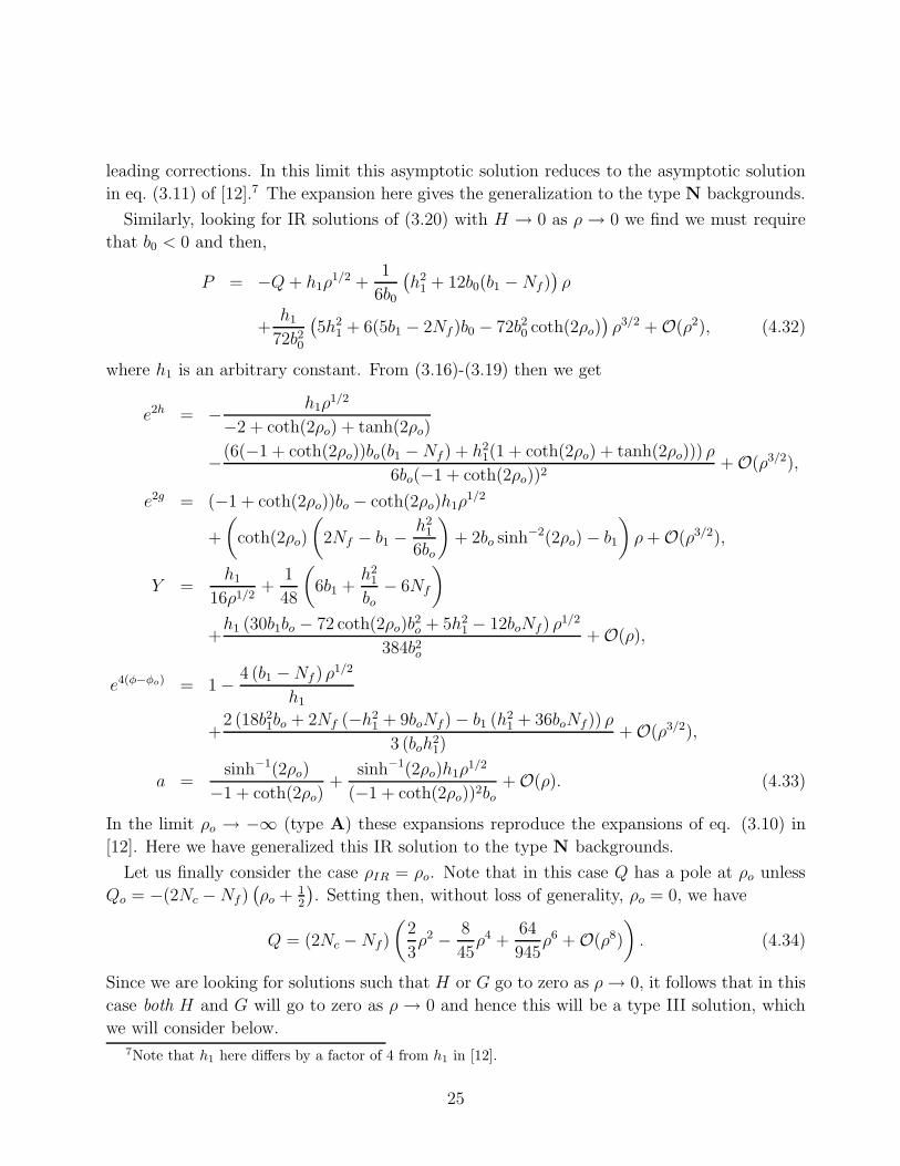
in eq. (3.11) of [12].7 The expansion here gives the generalization to the type N backgrounds.

Similarly, looking for IR solutions of (3.20) with H → 0 as ρ → 0 we find we must require

that b0 < 0 and then,

P = −Q+ h1ρ1/2 +

1

6b0

(h2

1 + 12b0(b1 −Nf))ρ

+h1

72b20

(5h2

1 + 6(5b1 − 2Nf )b0 − 72b20 coth(2ρo))ρ3/2 + O(ρ2), (4.32)

where h1 is an arbitrary constant. From (3.16)-(3.19) then we get

e2h = − h1ρ1/2

−2 + coth(2ρo) + tanh(2ρo)

−(6(−1 + coth(2ρo))bo(b1 −Nf ) + h21(1 + coth(2ρo) + tanh(2ρo))) ρ

6bo(−1 + coth(2ρo))2+ O(ρ3/2),

e2g = (−1 + coth(2ρo))bo − coth(2ρo)h1ρ1/2

+

(coth(2ρo)

(2Nf − b1 −

h21

6bo

)+ 2bo sinh−2(2ρo) − b1

)ρ+ O(ρ3/2),

Y =h1

16ρ1/2+

1

48

(6b1 +

h21

bo− 6Nf

)

+h1 (30b1bo − 72 coth(2ρo)b

2o + 5h2

1 − 12boNf) ρ1/2

384b2o+ O(ρ),

e4(φ−φo) = 1 − 4 (b1 −Nf ) ρ1/2

h1

+2 (18b21bo + 2Nf (−h2

1 + 9boNf) − b1 (h21 + 36boNf)) ρ

3 (boh21)

+ O(ρ3/2),

a =sinh−1(2ρo)

−1 + coth(2ρo)+

sinh−1(2ρo)h1ρ1/2

(−1 + coth(2ρo))2bo+ O(ρ). (4.33)

In the limit ρo → −∞ (type A) these expansions reproduce the expansions of eq. (3.10) in

[12]. Here we have generalized this IR solution to the type N backgrounds.

Let us finally consider the case ρIR = ρo. Note that in this case Q has a pole at ρo unless

Qo = −(2Nc −Nf)(ρo + 1

2

). Setting then, without loss of generality, ρo = 0, we have

Q = (2Nc −Nf)

(2

3ρ2 − 8

45ρ4 +

64

945ρ6 + O(ρ8)

). (4.34)

Since we are looking for solutions such that H or G go to zero as ρ→ 0, it follows that in this

case both H and G will go to zero as ρ → 0 and hence this will be a type III solution, which

we will consider below.7Note that h1 here differs by a factor of 4 from h1 in [12].

25

Type III:

Finally we look for IR solutions for which H → 0 and G → 0 in the IR. We again first

consider ρIR > ρo and we take ρIR = 0. In terms of the expansion (4.26) this requires that

b0 = 0. We then find,

P = h1ρ1/3 − 9Nf

5ρ− 2h1

3coth(2ρo)ρ

4/3 − 1

175h1

(50b21 − 18N2

f

)ρ5/3 + O(ρ2), (4.35)

where h1 6= 0 is an arbitrary constant. Evaluating the rest of the background functions we

find

e2h = −1

4h1 tanh(2ρo)ρ

1/3 +1

20tanh(2ρo) (9Nf + 5b1 tanh(2ρo)) ρ

+1

6

(1 +

3

cosh2(2ρo)

)h1ρ

4/3 + O(ρ5/3),

e2g = − coth(2ρo)h1ρ1/3 +

(−b1 +

9

5coth(2ρo)Nf

)ρ

+1

3(−5 + cosh(2ρo)) sinh−2(2ρo)h1ρ

4/3 + O(ρ5/3),

Y =h1

24ρ2/3− Nf

10− 1

9coth(2ρo)h1ρ

1/3 +

(−25b21 + 9N2

f

)ρ2/3

420h1+ O(ρ),

e4(φ−φo) = 1 +6Nfρ

2/3

h1

+3(5b21 + 39N2

f

)ρ4/3

5h21

+ O(ρ5/3),

a =1

cosh(2ρo)− b1 tanh2(2ρo)ρ

2/3

h1 sinh(2ρo)+

2 tanh2(2ρo)

sinh(2ρo)ρ+ O(ρ4/3). (4.36)

This expansion generalizes the type A III expansion of eq. (3.12) in [12] to the type N

backgrounds. Indeed, eq. (4.35) reproduces this expansion in the type A limit ρo → −∞.

Coming finally back to the case ρIR = ρo, we have seen that one should set Qo = −(2Nc −Nf)

(ρo + 1

2

)to avoid the pole in Q, which takes the form (ρo = 0) (4.34). Looking for

solutions with P → 0 as ρ→ 0, and noting that P should go to zero slower than Q to ensure

that both H and G remain positive, we find that there is a solution provided Nf = 0. Namely,

P = h1ρ+4h1

15

(1 − 4N2

c

h21

)ρ3 +

16h1

525

(1 − 4N2

c

3h21

− 32N4c

3h41

)ρ5 + O(ρ7), (4.37)

where h1 is again an arbitrary constant. This gives,

26

e2h =h1ρ

2

2+

4

45

(−6h1 + 15Nc −

16N2c

h1

)ρ4 + O(ρ6),

e2g =h1

2+

4

15

(3h1 − 5Nc −

2N2c

h1

)ρ2 +

8 (3h41 + 70h3

1Nc − 144h21N

2c − 32N4

c ) ρ4

1575h31

+O(ρ6),

Y =h1

8+

(h21 − 4N2

c ) ρ2

10h1

+(6h4

1 − 8h21N

2c − 64N4

c ) ρ4

315h31

+ O(ρ6),

e4(φ−φo) = 1 +64N2

c ρ2

9h21

+128N2

c (−15h21 + 124N2

c ) ρ4

405h41

+ O(ρ6), (4.38)

a = 1 +

(−2 +

8Nc

3h1

)ρ2 +

2 (75h31 − 232h2

1Nc + 160h1N2c + 64N3

c ) ρ4

45h31

+ O(ρ6).

This is a new IR solution with a ‘good singularity’ for the type N backgrounds in the flavorless

case. It should be interesting to study its dynamics.

4.4 Solutions of the BPS equations as RG flows

The solutions described in [9, 12] are a special case of the set of possible solutions to the

BPS equations, given the ansatz in eq. (3.1). We have seen that more general asymptotics

are possible, for large values of the radial coordinate ρ, the metric elements can grow as

H ∼ G ∼ Y ∼ e4ρ/3. Another possibility is that one of the elements of the metric can collapse

at a finite value of the radial coordinate, ending the space. In order to study how generic

these solutions are; we can make a qualitative analysis of the system of BPS equations as a

four-dimensional dynamical system. In the type A case the system is simpler and reduces to

three dimensions. We would like to interpret each solution as describing a different RG flow

in the space of holographic dual theories.

We will work with the ρ-dependent functions P = Ncp, Q = Ncq and u = (p2−q2)Y/Nc and

use the parameter x ≡ Nf/Nc. Using the first order equations in (3.12), with the constraint

27

(3.15) imposed, we can rewrite the BPS equations as,

p′ = −x+8u

p2 − q2,

q′ =2 − x

cosh τ− 2q sinh τ tanh τ,

u′ = 4u

[cosh τ − xp

p2 − q2− q

p2 − q2

(2 − x

cosh τ− 2q sinh τ tanh τ

)],

τ ′ = −2 sinh τ,

φ′ =xp

p2 − q2+

q

p2 − q2

(2 − x

cosh τ− 2q sinh τ tanh τ

).

(4.39)

Let us fix 1 < x ≤ 2,8 since the equations are independent of φ, the solutions can be described

as trajectories in the (p, q, u, τ) space. The trajectories are tangent to the vector field defined

by the values of (p′, q′, u′, τ ′). The BPS type A equations correspond to τ = 0. That is a

co-dimension one fixed subspace in the τ direction.

For physical solutions all the functions (appearing as warp factors in the metric) should be

positive, so p2 ≥ q2. When τ > 0, τ ′ < 0, so type N solutions flow from a finite or infinite

value of τ in the IR (ρ = ρIR) to τ = 0 in the UV (ρ → ∞). This is another way to see that

types A and N solutions have the same UV asymptotics. At fixed values of τ > 0 and u there

are three relevant curves in the (p, q) plane

p′ = 0 ⇒ p2 − q2 = 8ux, if p2 − q2 >

8u

x, then p′ < 0,

q′ = 0 ⇒ q = 2−x(2 sinh2 τ)

, if q >2 − x

(2 sinh2 τ), then q′ < 0, (4.40)

and the curve u′ = 0

(p− x

2 cosh τ

)2

− (1− 2 tanh2 τ)

(q +

2 − x

2(1 − sinh2 τ)

)2

=x2

4 cosh2 τ− (2 − x)2

4 cosh2 τ(1 − sinh2 τ).

(4.41)

where u′ > 0 above this curve (larger values of p). The curves q′ = 0 and p′ = 0 attract the

flow in the (p, q) plane. The curve q′ = 0 is independent of u and p and it disappears for A

solutions (τ → 0). However if x = 2 in the A solution, then q′ = 0 exactly. The curve p′ = 0 is

independent of τ and is a hyperbola in the (p, q) plane, asymptoting the lines p = ±q. When

u→ 0, the hyperbola approaches these lines. The curve u′ = 0 can be different conical curves

depending on the sign of the coefficient of the q2 term and therefore on the value of τ . For

2 tanh2 τ = 1, the curve is a parabola passing through (p = x/√

2, q = 0) and (p = 0, q = 0).

8 The analysis for x > 2 can be repeated using Seiberg duality Nc → Nf −Nc, H ↔ G that in this notationcorresponds to p→ (x− 1)p, q → −(x− 1)q, u→ (x− 1)3u and then use x = x/(x − 1), so 1 < x ≤ 2.

28

For larger values of τ , the curve is an ellipse, passing through (p = x/ cosh τ, q = 0) and

(p = 0, q = 0). When τ → ∞, the ellipse collapses to the point (p = 0, q = 0), so there is no

region where u′ < 0.

For smaller values of τ , the curve is a hyperbola. For low values of τ , one of the branches

passes through (p = 0, q = 0) but lies below the p = ±q > 0 lines, so it does not affect the

physical solutions. The other branch passes through the point (p = x/ cosh τ, q = 0). As we

increase τ , the two branches come closer until they merge at

sinh2 τ =4(x− 1)

x2, (4.42)

and form a new hyperbola where now the relevant branch passes through the points (p =

0, q = 0) and (p = x/ cosh τ, q = 0).

For solutions of type A (τ = 0), when Nf = 2Nc (x = 2) the p′ = 0 curve is a fixed line

for the flow in the plane defined by constant u (Fig. 1). The points where this curve intersects

the curve u′ = 0 are fixed points of the three-dimensional system, and they correspond to the

exact Nf = 2Nc solution found in [9, 12]. In terms of the original functions appearing in the

metric h = (p+ q)/4, g = (p− q)/4, the set of fixed points form a curve in the (h, g, u) space

that can be parametrized as

(h, g, u) =

(h,

h

4h− 1,

4h2

4h− 1

), ∞ > h > 1/4 . (4.43)

The fixed line only exists for Nf = 2Nc. In the notation of [9, 12], the line of fixed points is

parametrized by ξ = 1/h (see eq. (4.5)).

We can easily extend the analysis for a smaller number of flavors Nf ≤ Nc. There are two

main effects as x → 0. The first is the lift of the attractor region (4.40) towards infinity, so

it disappears completely when x = 0, and then p′ > 0 on the (p, q) plane. The second is the

modification of the u′ = 0 curve. When x = 1, the merging of the two branches of the low τ

hyperbola occurs at τ = 0. Then, the u′ = 0 curve is a straight line p = q + 1 on the physical

region and also at the border p = −q > 0. The region p > q + 1 corresponds to u′ > 0, while

q + 1 > p > q > 0 corresponds to u′ < 0. When x < 1, the u′ = 0, τ = 0 curve is a hyperbola

passing through the points (p = 0, q = 0) and (p = x, q = 0) and asymptoting p = q + 1.

In Section 4.3 we have presented the possible asymptotic behavior of solutions as a function

of the radial coordinate ρ. We will comment on them under the perspective of flows in the

dynamical system defined by (4.39).

Let us start with the UV behavior ρ → ∞. As we have already commented, both N flow

towards the τ = 0 fixed plane, where A solutions live, so they have common asymptotics.

There are two possible classes of asymptotics (see Section 4.3.1).

• For class II all functions grow exponentially, so this corresponds to a situation where

the flow is in the u′ > 0 region and the attractor p′ = 0 moves towards infinity. The

29

h

g

h

g

(a) (b)

Figure 1: We represent the flow in the (p, q) plane at fixed u and τ = 0 (type A solutions). Thephysical region is above the black lines p = ±q > 0. (a) The RG flow for Nc < Nf < 2Nc. Thep′ = 0 line (red) acts as an attractor for the flow, the dark lines are the limits of the attractor regionh′ = 0 and g′ = 0. The u′ = 0 line (blue) has also been represented. (b) The RG flow for Nf = 2Nc.The p′ = 0 (red) and u′ = 0 (blue) lines have been represented. There are two fixed points of theflow at the intersection of the two curves.

attractor q′ = 0 will move towards positive or negative values of q depending on the

value of Nf . The flow will try to reach the intersection of both. This is a very generic

situation.

• Class I solutions, on the other hand, correspond to cases where the flow is in the u′ < 0

region, so the p′ = 0 attractor is dragged towards the lines p = ±q. Generically, the flow

would hit the lines and the solution will end at a finite value of the radial coordinate,

so the corresponding solutions will have a boundary. Class I solutions are very special,

because they correspond to a situation where u′ → 0− asymptotically, so they are just

marginal solutions between class II solutions and solutions with boundary. In the special

case of Nf = 2Nc there is no flow in the q direction, so the flow will hit the fixed line

p′ = 0, u′ = 0. Notice that this is still a very special situation, usually the flow will miss

the fixed line and go to a class II solution.

Let us examine now the IR behavior. Depending on the solution we can have ρ → 0 (for

either ρ0 < 0 or ρ0 = 0) or ρ → −∞. The first case corresponds to type II and III, while the

last corresponds to type I (see Section 4.3.2). In terms of the dynamical flow, the meaning is

the following

• Type I: It corresponds to flows coming from infinity in the (p, q) plane, starting at the

fixed subspace u = 0. Notice that they are always in the u′ > 0 region for N solutions or

for A solutions when Nf > Nc. However, when Nf ≤ Nc, the u′ = 0 curve on the (p, q)

30

plane is different and can go to infinity. When Nf = 2Nc it is also possible to have flow

starting at the fixed line p′ = 0, u′ = 0, an example of this is the exact solution (4.7),

that then runs into class II UV asymptotics. Notice that this is possible because the

fixed line is not an attractor in all directions, it rather corresponds to a ‘saddle point’

in the flow.

• Type II and III: If ρ0 < 0, they correspond to flows starting on the p = ±q lines, with

type III corresponding to the point p = q = 0. If ρ0 = 0, then solutions have to start on

the q′ = 0 line (q = 0) at τ = ∞.

A final comment is on the enlargement of the u′ < 0 region for Nf ≤ Nc. Flows on that region

are more likely to hit the p = q line, thus corresponding to a solution with boundary. From

the field theory perspective this may correspond to the runaway behavior of the N = 1 SQCD

theory when an ADS superpotential is generated. In the theories we consider here there is

also a quartic superpotential, so the theory can show a different behavior.

5 Physics of the new solutions

In this Section we will study some aspects of the non-perturbative physics encoded by the new

solutions we presented in Section 4. We will start with general comments, then we concentrate

on aspects that involve the IR physics, hence using the IR (small ρ) expansions derived in

Section 4, and then we will move into some observables computed with the UV expansions

(ρ → ∞). Some of the computations we will perform to calculate non-perturbative effects,

have been thoroughly checked in the past, using different backgrounds with or without flavors;

in those cases, we will be brief in our presentation. In contrast we will give details when new

material is presented.

5.1 General Comments on the Field Theory

Let us first study an aspect that does not refer to the UV or the IR of the QFT, that is Seiberg

duality [17].

It is by now well understood that for the particular field theories in the class that we are

considering see eq. (2.4), Seiberg duality is not just the infrared equivalence of two theories,

but the duality is valid all along the flow. This peculiar behavior is due to the presence of the

quartic term in the quarks. Basically the argument is that when Seiberg dualized,

W ∼ κ(QQ)2 = κMM →Wdual ∼ κMM +1

µqMq, (5.1)

where M is the meson superfield and q, q are the dual quarks. Now, the presence of the M2

term-a mass term- allows us to integrate out the meson, leaving us with a superpotential of

31

the form

Wdual ∼1

κ(qq)2, (5.2)

then, the theory is Seiberg dual to itself. This, by the way, is at the root of the working of

the Klebanov-Strassler duality cascade. See the lectures [18] for lucid explanations.

How is the previous discussion reflected by our backgrounds? This was discussed at length

in [12]. Here, we can briefly mention that our generalized BPS eqs. (3.12) and our Hamiltonian

eq. (3.8) do indeed show an interesting symmetry. Indeed,

P → P, Q→ −Q, τ → τ, Y → Y, σ → −σ, Nc → Nf −Nc, (5.3)

is an invariance of the equations, the Hamiltonian and the Hamilton-Jacobi principal function

in eq. (3.10). This implies that if we find one solution, we have by replacement in eq. (5.3)

found another one with the correct relations between color and flavor groups.

The U(1) R-symmetry of the QFT is associated with translations in the angle ψ. The

breaking of the symmetry will be briefly discussed later, but this point together with the

matching of global anomalies does not present any subtlety aside from what was discussed in

[12].

As was proposed in the paper [23] the gaugino bilinear is related to the function b(ρ) that

appears in the RR three form. We will keep that identification that will allow us to write an

energy-radius relation (in the UV)

e2ρ3 =

µ

Λ, (UV, ρ→ ∞). (5.4)

Using the information above, one can easily obtain that the solutions whose UV asymptotics

is given in eqs. (4.15)-(4.16)-(4.17) represent the field theory described in Section 2, once

a dimension six operator is added. The addition of this irrelevant term in the Lagrangian

(like in a related example of [19, 20]) dramatically changes the UV of the field theory leading

to a solution that is ‘away’ from the near horizon of the D5 branes. We believe that this

irrelevant operator is related to the gauge sector, for instance O6 = (WαWα)3/2 ∼ (Fµν)3,

or O6 ∼ (DµFνρ)2, though there could be also operators related to the KK multiplets like

O6 = |Φk|6, etc. Our proposal that the irrelevant term is made out of operators transforming

in the adjoint of the gauge group is due to the fact that the asymptotic eqs. (4.15)-(4.16)-

(4.17) exist also in the case of Nf = 0. The field theory aspects in the flavor-less case were

studied and the solution was (numerically) found in Section 8 of [9].

Let us proceed by studying aspects of the IR of the field theory, encoded in the backgrounds

of Section 4.

32

5.2 Physics in the Infrared

As stated above, we will start by studying non-perturbative effects that the backgrounds

encode in the small radius region (ρ → 0)9. We will also comment on Wilson, ’t Hooft

and dyon loops, domain walls and the behavior of the quartic coupling in the field theory

described in eq. (2.4). Finally we will give a general analysis to find what are the conditions

that determine if an object is screened in the dual theory.

5.2.1 Enhancement of the flavor group

In this section we describe something that applies equally to the solutions discussed here and

the ones in [9] and [12]. We can ask the following question: what is the dual flavor group?

The first answer may be that the group is SU(Nf ), but a better analysis shows that actually

the flavor branes are separated-this is an effect of the smearing-so, a more likely answer is that

the group is U(1)Nf . Many dynamical aspects will not depend on this and it may happen that

if the distance between branes is vanishing (for example in the IR) then, the strings stretching

between flavor branes become massless and the SU(Nf ) symmetry is recovered in that regime

of energies. The fact that the F1-strings stretching between flavor branes have a mass has

important consequences regarding the existence-or not- of diagrams that could likely correct

the BI-WZ action that we used for the flavor branes.

To analyze this, we will proceed as follows. We will compute the volume of the space Σ4 on

which we smear the flavor branes. We will divide this by Nf and associate a given “volume

per flavor brane”. We will then propose that the distance between flavor branes is given by

the fourth root of such ‘volume per flavor brane’ and estimate the mass of the F1-strings as

the string tension times this quantity.

We also need to estimate the proper energy Eproper of an object in the bulk, given the energy

of the dual object in the field theory EQFT . The relation is

EQFT =√gttEproper = eφ/2Eproper. (5.5)

Due to the dependence of the dilaton on the radial position, if we keep the QFT energy fixed,

then the proper energy of the mode must vary. If the proper energy grows very fast in the

IR, it could be possible to excite strings between different branes even if they are at a finite

separation, leading to an enhancement of the flavor group to SU(Nf ).

Let us see the computation. We focus first on type A solutions. In the string frame, the

induced metric on the four cycle Σ4 is,

ds2Σ4

= eφ[H(ρ)(dθ2 + sin2 θdϕ2) +G(ρ)(dθ2 + sin2 θdϕ2) + Y (ρ)(cos θdϕ+ cos θdϕ)2

]. (5.6)

9For convenience we are taking the IR region to be at ρ → 0, but as explained above, in general it is atρ→ ρIR

33

So, the volume to be computed is

V4 =

∫dθdθdϕdϕ

√gΣ4 =

4π2e2φ√HG

∫dθdθ

√HG sin2 θ sin2 θ + Y G cos2 θ sin2 θ +HY cos2 θ sin2 θ. (5.7)

So, we need to look for the values of this integrals in the IR. Indeed, in the UV, is clear from

the asymptotic expansions, that this integral will indeed diverge, making the mass of the F1s

to diverge. The group is then broken to U(1)Nf in the UV. In the IR, the analysis depends

on the type of solution we consider. Let us first analyze this for the three types of IR type

A solutions of the SU(Nc) dual background in [12]. They were called type I, II, and III IR

behaviors. In type I and II, the previous volume is constant, indicating that there will be a

fixed separation between flavor branes. In the type II case, the dilaton goes to a constant, so

at very low energies, the strings between branes will decouple, breaking the flavor group to

U(1)Nf . In type I the dilaton vanishes, so the proper energy grows unbounded in the IR and

the group gets enhanced to SU(Nf ). In type III, we observe that the volume vanishes, also

enhancing the flavor group.

A similar analysis can be done for the type N solutions, using the determinant of the induced

metric in the far IR. Given the expansion for type N solutions in Section 4, we obtain that

for type I and II the volume diverges at ρ = 0 and the dilaton is constant. This implies that

non-diagonal strings are very massive and do not contribute to processes in the IR physics.

The flavor group is then broken to U(1)Nf by the solutions. This is basically the reason why

in the Introduction we proposed different couplings between quark superfields and adjoint KK

modes see eq. (2.3)-the difference may be just a phase factor for different positions of branes

in Σ4. In type III solutions on the other hand, the volume vanishes in the IR and the flavor

group gets enhanced to SU(Nf ).

5.2.2 String-like objects

It is known that the holographic dual to the Wilson loop corresponds to a fundamental string

describing the 4d Wilson loop in the Minkowski directions, exploring the radial directions and

ending on a brane at spatial infinity [21], while in the type of backgrounds that are not S-

duality invariant, the ’t Hooft loop is computed by a D3 brane wrapping a topologically trivial

two-cycle. These string-like objects should have only a finite length due to the screening from

fundamental matter.

In the case of type A backgrounds, it was shown that depending on the IR of the solution,

different vacua of the QFT present distinctive behavior for Wilson and ’t Hooft loops, see

Sections 4.4 and 4.5 of the paper [12] for a detailed analysis. Indeed (always in the case of

type A backgrounds) it was seen that in type I solutions the Wilson loop tension vanishes,

while it is finite for type II and III. On the other hand, the tension of the ’t Hooft loop vanishes

34

only for type III solutions. Therefore, type I solutions correspond to a Higgs phase, while type

III correspond to confined phases. In type II both quarks and monopoles are confined, so it

should correspond to a oblique confined phase, where dyons with both electric and magnetic

charge should be free.

Wilson loops In a QFT with fundamental matter, the QCD-string can break, basically

due to pair creation. This effect is offset if one is working in the quenched approximation

(Nf

Nc∼ 0). Our backgrounds do indeed capture screening effects as was seen in [9, 12], by the

existence of maximal length for the quark-antiquark separation. Nevertheless one can get an

intuitive idea about the way a quark pair interacts by looking at the QCD string tension in

the far IR. This is computed in the string duals by the value of the quantity (see [22] for a

summary)

TQCD =√gttgxx|ρIR

. (5.8)

We can see that this quantity is non-zero for the three types of IR asymptotics of type N

backgrounds. Indeed, it is just proportional to the value of eφ(ρIR); this indicates that at low

energies, the pair feels a linear potential10. Contrast this with the type A backgrounds where

for asymptotics of type I the force was vanishing. The main difference between type A and

type N backgrounds resides in the existence of the functions a(ρ), b(ρ) that as was discussed

in the literature [23], can be associated with the formation of a gaugino condensate. This

seems to be at the root of the different behavior for the QCD string tension.

Let us now study another gauge invariant observable, the ’t Hooft loop.

’t Hooft loops As discussed previously in the literature, for backgrounds that are not

invariant under S-duality like the present ones, the ’t Hooft loop is computed via a D3 brane

that wraps a two cycle in the internal space. The manifold on which the D3 is proposed to

extend is,

Σ4 = [x, t, θ = θ, ϕ = 2π − ϕ, ψ = π, ρ(x)]. (5.9)

The induced metric for a D3 on that manifold is

ds2ind = eφ

[− dt2 + dx2(1 + e2kρ′2) + (e2h +

e2g

4(a− 1)2)(dθ2 + sin2 θdϕ2)

]. (5.10)

After integrating over the internal manifold, the ‘effective string’ (representing the ’t Hooft

loop) has an action,

Seff = 4πTD3

∫dxeφ(e2h +

e2g

4(a− 1)2)

√(1 + e2kρ′2) =

∫dxTeff

√(1 + e2kρ′2). (5.11)

This effective tension Teff plays a similar role to that of the QCD-string tension in the previous

subsection. This object can be studied in the IR (again, keeping in mind that the ’t Hooft

10Of course, at even longer distances, screening takes place and the potential changes.

35

loop will also present screening effects at even lower energies) to get an intuitive idea of the

force, at low energies, between a pair of monopoles.

We obtain using the type N IR expansions that for type I and type III backgrounds the

effective tension vanishes, leaving the monopoles free. In contrast, for type II backgrounds

the effective tension is constant, leading to a linear potential between them.

It is a natural next step, to compute the tension between a pair of dyons. We are not

aware of a concrete computation to calculate this effect, then we will propose one. So, we

propose that the dyon-anti-dyon is represented by a D3 brane extended on (t, x) wrapping the

topologically trivial cycle,

θ = θ, ϕ = 2π − ϕ , (5.12)

and that is charged by the presence of a world-volume electric field Ftx. We will show that

for a particular value of the electric charge, the tension of the dyon loop indeed vanishes, in

agreement with the oblique confinement picture. We will do this in the case of the simpler

type A backgrounds for illustrative purposes.

Computing dyon-antidyon loops Since, as stated above, we believe this is new material,

we will be more detailed. We study the proposal in type A and then (briefly) in type N

backgrounds. In type A configurations, the induced metric, RR three form and world-volume

fields on the D3 brane described around eq. (5.12) is (the brane also extends in the radial

direction ρ(x)),

ds2ind = eφ

[− dt2 + (1 + 4Y ρ′2)dx2 + (H +G)(dθ2 + sin2 θdϕ2)

],

Ftx = ∂tAx,

F3 = d[(2Nc −Nf)

4(ψ − ψ0) sin θdθ ∧ dϕ

]. (5.13)

We then compute the Born-Infeld part of the action,

det[gab + 2πFab]1/2 = e2φ(H +G) sin θ

√1 + 4Y ρ′2 − 4π2e−2φF 2

tx. (5.14)

After integrating over the sphere directions and considering the WZ term that appears because

of the presence of a nontrivial C2 on the worldvolume, the action for the D3 brane is,

S = −4πTD3

[ ∫dxeφ(H +G)

√1 + 4Y ρ′2 − 4π2e−2φF 2

tx − ΘFtx

], (5.15)

where Θ is given by Θ =2Nc−Nf

4(ψ − ψ0). We then compute the eq. of motion for the gauge

field, obtaining

Ftx = − eφ(Θ − Θ0)√

1 + 4Y ρ′2

2π√

4π2(H +G)2 + (Θ − Θ0)2, (5.16)

36

where Θ0 is an integration constant. Replacing back into the action (5.15), we get

S = −4π

∫dx Teff

√1 + 4Y ρ′2, (5.17)

which is the action for an ‘effective string’ that is what we consider to be the QCD string (for

dyons), with tension given by

Teff = 2πTD3eφ

[(H +G)2 + Θ(Θ − Θ0)

]

√4π2(H +G)2 + (Θ − Θ0)2

. (5.18)

We can see that the dyon-anti-dyon tension depends on the type of solutions we deal with.

Always thinking in the case of type A configurations and using the asymptotic expansions

derived in [12], we see that for type I the tension is always finite, so the dyons are confined.

For type III the tension vanishes only when Θ0 = Θ (which means that Ftx = 0) or Θ = 0. In

both cases, the dyon has no electric charge and becomes a monopole. For type II theories, in

the IR H + G → |C| (constant). If we choose Θ0 conveniently, then the tension of the dyon

vanishes. So, for each of the type II solutions and its Seiberg dual, a dyon with a precise value

of the electric charge is free. Notice that a shift in Θ changes the value of the electric charge

of the free dyon, so the oblique confined phase is different, this is what we expect from field

theory.

Having finished with the possible string-like objects (to which we will come back for a more

general analysis in Section 5.2.5), we would like to study now higher dimensional defects.

5.2.3 Domain-wall tensions

A domain wall in these backgrounds is represented by a D5 brane that wraps (in a SUSY

preserving way) a three-cycle and extends in three of the four Minkowski directions, preserving

SO(1, 2). The proposed manifold on which the five brane extends was given in [9] is

Σ6 = [t, x1, x2, θ, ϕ, ψ]. (5.19)

The effective tension of this (2+1)-dimensional object-that is after integration over the internal

three manifold- is

Teff,DW = 16π2e2φ+k(e2h +e2ga2

4). (5.20)

The IR behavior of this quantity is such that the effective tension is constant for type I and

type III solutions, while is divergent for type II asymptotics. This means (in the case of type II

solutions) that the domain-wall like object has to sit at a finite value of the radial coordinate,

where its tension is minimized. We move now to the study of our last IR observable, the value

of the quartic coupling in the different asymptotics.

37

5.2.4 Quartic coupling

In the paper [12] a possible definition for the quartic coupling κ between quark superfields in

the QFT has been proposed. The definition is just based on dimensional analysis and has the

right UV beta function, but does not transform correctly under Seiberg duality. We would

like to propose here a different definition with the right properties

log κ2 =V ol[S3] − V ol[S3]

V ol[S1] × V ol[S2]= −e

2h + e2g

4(a2 − 1)

e2h + e2g

4(a− 1)2

= −QPeτ (5.21)

For type A backgrounds log κ2 = (G − H)/(G + H). Seiberg duality interchanges the two

three spheres in the metric, that in (5.21) is seen as κ→ κ′ = 1/κ. In self-dual configurations

H = G, κ = κ′ = 1. Let us stress again that this choice is based on some general properties

but we do not have a proof of it being the actual quartic coupling of the dual field theory.

Analyzing the behavior of this quantity in the case of type A and N backgrounds, we see

that κ always goes to a constant value in the IR or UV. In type A III, N I and N III infrareds

and in class II ultraviolets, it flows to the self-dual value κ = 1.

5.2.5 Screening as string breaking

In the papers [9] and [12] it was explicitly shown (using the dual backgrounds) that due to

the presence of the fundamental matter, different ‘loops’ (Wilson, ’t Hooft, dyon) may present

a maximal length, indicating screening. In this Section, we would like to present a general

study whose outcome is a sufficient condition for which a finite maximal length will occur (or

not). Our analysis will not depend on a particular asymptotics. Let us emphasize that, while

the existence of a maximal length implies screening, the existence of an infinite length does

not imply confining behavior. We are considering the “connected” Wilson loop and its energy

must be compared with the possible “disconnected” solution indicating creation of pairs and

screening-for another example where the same comment applies see [25]. The energetically

favorable solution will be physically realized.

Let us then examine the issue of the maximal length of string-like objects described by a

string/brane extending on t, x and wrapping the internal space. The bulk radial coordinate

is ρ, and the profile of this object is described by the function ρ(x). If the metric is

ds2 = eφ(ρ)(−dt2 + dx2 + 4Y (ρ)dρ2) + gαβ(ρ, y)dyαdyβ, (5.22)

with gαβ the metric of the internal space, then the Lagrangian coming from the Born-Infeld-

Wess-Zumino action, after integration over the internal directions yα, will have the general

form,

L = T (ρ)√

1 + 4Y ρ′2, (5.23)

38

where T (ρ) is the effective tension of the brane that depends in general on the dilaton and the

components of the metric in the directions of the internal space that the brane is wrapping.

The usual analysis goes as follows: we first define the Hamiltonian, that is a conserved quantity

H =∂L∂ρ′

ρ′ −L = − T√1 + 4Y ρ′2

≡ −T0. (5.24)

If for some value of ρ = ρ011 the profile ends smoothly ρ′ = 0, then T0 = T (ρ0). From this

expression, it is straightforward to find

dx

dρ=

2√Y T0√

T 2 − T 20

. (5.25)

In order to have a sensible (real-valued solution), we need that T > T0 over all the brane (we

are assuming that all quantities are positive). So,

• If the tension is a growing function of the radial position T ′(ρ) ≥ 0+ as ρ → ρ0, then

the solution exist for ρ > ρ0.

• If the tension is a decreasing function of the radial position T ′(ρ) ≤ 0− as ρ→ ρ0, then

the solution exist for ρ < ρ0.

Physically, this means that the object extends towards values where its tension is smaller. In

the backgrounds we are considering we have usually dilaton factors that grow exponentially

in the tension as ρ→ ∞, hence the branes will ‘hang’ from the UV towards the IR. However,

close to the singularity, some functions of the metric grow and some functions decrease, so

in principle there could be objects that cannot go beyond some finite value of the radial

coordinate, and there could be objects that extend from the singularity towards the UV,

although they cannot go arbitrarily far. When this happens, the objects will have a finite

tension, the region where T ′ = 0 acting as an effective IR wall for them. Let us analyze these

cases in detail.

The simpler case is when there is no IR wall and the far IR is at ρ = 0, so we can use the

asymptotic expansions. Let us assume that the tension of the object vanishes in the IR as

some power T ∼ ρb, b > 0. Also, we assume that the function Y also has some power-like

behavior, but can vanish, be a constant or blow up like Y ∼ ρa. Then, the equation of motion

in eq. (5.24) reads,dx

dρ∼ ρa/2ρb0√

ρ2b − ρ2b0

. (5.26)

11Notice that in this Section ρ0 denotes the turning point of the string-like object and should not be confusedwith the quantity defined earlier ρo that is the lowest value of the coordinate ρ in the background. The contextwill make this clear.

39

Close to the tip, ρ ≃ ρ0(1 + ǫ). We can integrate trivially on ǫ to find a square root behavior,

so the profile at the tip looks like

x(ρ) ∼ ρ(1+a)/20

√ρ− ρ0. (5.27)

The criterion we will adopt to quickly evaluate the ‘length’ of the putative loop is the following:

the factor in front of the square root determines how “open” is the configuration. If the

configuration is to reach infinite length in the x direction when the object explores the far IR

of the dual theory, then this factor should diverge when ρ0 → 0. In the case at hand, this

implies that a < −1. This is indeed the case of the AdS string, where T ∼ ρ2 and Y ∼ ρ−4.

The next possibility is to consider an object that has finite tension, so that T ∼ T∗ + cρb,

b > 0, c > 0 (this is necessary to have T ′ > 0) when ρ → 0. Now the equation of motion is a

bit differentdx

dρ∼ T∗ρ

a/2

√(T∗ + cρb)2 − (T∗ + cρb0)

2∼ T

1/2∗ ρa/2√ρb − ρb0

. (5.28)

The profile at the tip now looks like

x(ρ) ∼ T 1/2∗ ρ

(1+a−b)/20

√ρ− ρ0. (5.29)

For example, we can analyze the previous expression for the case of the flavorless solution

(Nf = 0) in eq. (4.2), and check that this gives a = 0, b = 2 implying an infinite length. As

another example, we analyze the IR of type A backgrounds. In order to have an object that

can extend to infinite length, we should have that b > 1/2 in type II and b > 1/3 in type III.

Notice that the monopoles and dyons have b = 1/2 and b = 1/3, so they are screened objects.

Suppose now, that we have an object that feels an effective IR wall at ρ = ρ∗ where the

tension is minimized, so T ′(ρ∗) = 0 and T ′′(ρ∗) > 0. We are assuming that the background

at this point is smooth, and the functions of the metric do not vanish, so Y and the tension

admits Taylor expansions

T = T∗ + T2(ρ− ρ∗)2 + . . . , T2 > 0,

Y = Y∗ + Y1(ρ− ρ∗) + . . . . (5.30)

We take a configuration where the object ends smoothly at some point ρ0 > ρ∗ and consider

the limit ρ0 → ρ∗. It is convenient to use the coordinate r = ρ − ρ∗ and r0 = ρ0 − ρ∗ so

eq. (5.25) becomes,

dx

dr∼

√Y∗T∗√

(T∗ + T2r2)2 − (T∗ + T2r20)

2∼√Y∗T∗T2

1√r2 − r2

0

. (5.31)

Close to the tip, r ≃ r0(1 + ǫ). We can integrate trivially on ǫ to find a square root behavior,

so the profile at the tip looks like

x ∼√Y∗T∗T2

r−1/20

√r − r0. (5.32)

40

Therefore, when the tip of the object comes close to the IR wall r0 → 0, the length diverges.

It should be interesting to extend the analysis of this Section to the case in which we have

massive quarks; because it could provide more hints on the first order phase transition-in

terms of the mass- that occurs for the connected part of the Wilson loop, see [25]. Also,

it may be interesting to use the results of this Section to improve models of AdS/QCD to

incorporate screening effects. To close, let us mention that it should be nice to provide a link

between the formalism developed here and the ideas presented in [24].

Let us now move to study aspects of the UV of the field theory, using the large ρ region of

the solutions.

5.3 Physics in the Ultraviolet

Let us briefly study how some aspects of the UV field theory are captured by the backgrounds.

R-symmetry anomalies will be treated in a sketchy way. The results are similar to those in

[9] and [12]. The study of beta functions will be more detailed because it will shed light on a

long-standing puzzle.

The way the R-symmetry anomaly will work, as explained at length in [9] and [12] does

not change here. Basically this is because it only depends on the form of the RR field F3

when restricted to a particular manifold-see eq. (5.12)-considered at large values of the radial

coordinate. The result is not changed when switching between the different UV solutions we

found in Section 4.

Let us then concentrate on the beta function of the field theory as computed by the two

different UV expansions. We will present details, as this will teach us something interesting

about the field theory and its UV completion.

5.3.1 Beta function

A definition of the gauge coupling in the dual QFT in terms of type IIB objects was given in

[26]. Using that definition, we have an expression for the gauge coupling that reads,

8π2

g2= 2(e2h +

e2g

4(a− 1)2) = e−τP. (5.33)

As mentioned above, the relation between the scale of the QFT and the radial coordinate was

also proposed in [23] and [26]. This relation comes by associating the functions a(ρ) and/or

b(ρ) with the VEV of the gaugino condensate. One gets,

e2ρ3 =

µ

Λ, (UV, ρ→ ∞). (5.34)

We have found two types of UV behavior. One of them was already studied in [9] and [12]. The

other, for the solutions that asymptote to the conifold, was given in eqs. (4.15)-(4.16)-(4.17).

For both asymptotics, the relation in eq. (5.34) above holds.

41

This allows us to compute the behavior of the beta function in the UV of the QFT. The

results are that for the UV expansions presented in [9] and [12] we get (for Nf < 2Nc as

explained in those papers) that

β 8π2

g2=

3

2[2Nc −Nf ], (5.35)

that is the result expected from the NSVZ beta function, in the case in which the anomalous

dimension of the quark superfield is γQ = −12. See [12] for various consistency checks on this

value of the anomalous dimension.

Now, this is the puzzle: how is it possible that a theory with so many extra fields (in the

UV, the extra modes should be integrated-in) presents a beta function that adjusts so well

to the exact treatment of NSVZ. The comparison with the result obtained using the other

possible UV solution will illuminate this point. This also applies to the case Nf = 0 and we

believe it answers the criticism to the papers [26].

The beta function for a 6d theory The set-ups described in the Introduction are the

holographic duals of the six-dimensional field theories living on the D5 branes that wrap a

2-cycle of the deformed conifold. The dimensionful gauge coupling can be read from the D5

brane action g26 = α′gs, and one can define the dimensionless coupling

g62 = µ2g2

6Z2(µ) , (5.36)

where µ is some mass scale and Z(µ) is the renormalization factor of the 6d coupling, analogous

to a mass renormalization factor. The theory is perturbatively non-renormalizable, in the sense

that radiative corrections can generate an infinite set of irrelevant operators as the theory flows

to the UV. From a four-dimensional perspective, we can define a (dimensionless) coupling

g24 =

1

L2g26Z

2(µ) , (5.37)

where L2 ∼ Ncα′ is the size of the 2-cycle. In this case, the beta function is

β 8π2

g24

= −16π2

g24

d logZ

d logµ≡ −16π2

g24

γg , (5.38)

At one-loop in perturbation theory, the infinite tower of extra states (KK modes) would

generate a power-like running of the coupling in the UV

g24 ∼ 1

(Lµ)2. (5.39)

If we integrate out the KK modes, then an effective coupling for an irrelevant operator of

dimension six would be generated, also modifying the running of g4. As the energy scale

42

becomes of the order of the Kaluza-Klein mass, more irrelevant operators would enter, making

the theory non-renormalizable.

However, a six dimensional theory could be renormalizable at a non-perturbative level. This

is possible if there is a UV fixed point, as was shown in [27]. Looking at the beta function

(see Kazakov’s paper in ref. [27])

β 8π2

g26

= −16π2

g26

(1 + γg) , (5.40)

we see that a UV fixed point corresponds to an anomalous dimension γg = −1. On the

other hand, the four dimensional coupling would have the same running as the one-loop

perturbative result, suggesting that only a dimension six operator is generated, instead of an

infinite set of irrelevant operators. We can take this as an indication that the UV theory is truly

six dimensional, where such operator is marginal. It has been suggested that the marginal

operator respects scale invariance but not the full conformal invariance of the theory.

We can now see how this picture emerges in the holographic description. Using the pre-

scription of [26], we can see that the renormalization factor Z2 is proportional to the inverse

size of the cycle. In the UV, the relation between the radial coordinate ρ and the scale µ is

given as explained above by eq. (5.34). Then, for the solutions asymptoting to the conifold,

eqs. (4.15)-(4.16)-(4.17), we have

logZ = −2

3ρ = − log

µ

Λ⇒ γg = −1 . (5.41)

So the growing solutions correspond to six dimensional theories flowing towards a UV fixed

point. Let us examine the metric in the far UV, keeping only the leading asymptotics and

using the coordinate 2r = 3e2ρ/3, the background in eq. (2.13) with the asymptotics (4.15)-

(4.16)-(4.17) will read,

ds2 = eφ0[dx2

1,3 +4c+3

(dr2 + r2T 1,1)]

(5.42)

There is a scaling symmetry; we can rescale the coordinates r → λr, xµ → λxµ . This changes

the metric only by a conformal factor, that can be absorbed in the dilaton. Notice that the

RG flow is independent of the value of the dilaton. There is also a self-similarity relation

between different RG flows in the UV, since the transformation r → λr, c+ → λ−2c+ , leaves

the metric invariant.

The special solutions with UV given in [12] -see eqs. (4.9)-(4.13)- have a rather different

behavior. The renormalization factor goes as

logZ ∼ −1

2log ρ ∼ −1

2log log

µ

Λ. (5.43)

This gives the anomalous dimensions and gauge couplings

γg = − 1

2 log µΛ

⇒ g24 ∼ 1

log µΛ

, g26 ∼ µ2

log µΛ

. (5.44)

43

The running of the g4 coupling is exactly the one of a four dimensional N = 1 theory. This

is quite surprising, since a six dimensional theory is showing a completely four dimensional

behavior. From the string theory point of view, the six-dimensional solutions (5.42) look as a

decompactification limit and actually the metric coincides with the metric ‘outside’ the near-

horizon region of the 5-branes 12. Notice that the dilaton goes to a constant, so the energy

of probes in the gravitational background is simply proportional to the energy in the field

theory-see eq. (5.5)- and the extra dimensions can be easily explored.

On the other hand, in the ‘four dimensional solutions’ eqs. (4.9)-(4.13) the dilaton factor

in the proper energy formula (5.5) grows exponentially with the radial coordinate, while the

relative size of the compact dimensions grows only linearly. Then, for an object with fixed

energy in the field theory, the proper energy in the string dual is exponentially suppressed at

larger values of the radial coordinate in such a way that the wavelength will grow much faster

than the size of the compact dimensions. Therefore, it is very difficult to explore the extra

dimensions and the theory remains four-dimensional even in the ultraviolet.

In the dual field theory, the interpretation is that these backgrounds correspond to RG flows

where the six dimensional irrelevant operator is not generated, so they are renormalizable not

only in the six dimensional sense but also in a four dimensional sense. All these comments

are consistent and provide a different view on the findings in [28], where it was shown that

the beta function of the unflavored background was unaffected by the KK modes. For a field

theory argument that complements this one, see Appendix A.

Let us now analyze another contribution of this paper. The extension of these set-ups to

the case of orthogonal groups.

6 The case of SO(Nc) gauge group

In this Section we address some aspects of the version of SQCD described in Section 2.1, but

in the case in which the gauge group is SO(Nc). The best places where the field theory is

described are, for the pure SQCD case in [31] and the paper [32] for the theory that is more

like the one we are interested in. For a recent analysis of a field theory related to ours in

non-critical strings set-up see [30].

The N = 1 theory with orthogonal group has a rich phase structure, with fixed infrared

conformal points for 32(Nc − 2) < Nf < 3(Nc − 2) and a free magnetic dual description for

Nc−2 < Nf ≤ 32(Nc−2). For Nf < Nc−2 there is a dynamically generated superpotential of

the ADS type, associated to gaugino condensation. For Nf = Nc−4 and Nf = Nc−3 there is

also an extra branch with no superpotential. In the field theories described by the holographic

duals we study, this picture is modified by the presence of a classical superpotential coming

from the reduction from the six dimensional theory.

12As predicted to happen in a different context in the papers [19, 20]

44

The dual geometry is based on the same 5-brane construction wrapping a 2-cycle of the

resolved conifold. In order to have an orthogonal gauge group, we introduce an orientifold O5

plane parallel to the 5-branes. This setup was studied in [29]; the case of symplectic groups was

also addressed there. The orientifold has the effect of making a reflection on the orthogonal

directions, so the S3 surrounding the 5-branes becomes a projective space S3 → RP 3. When

we go from the brane picture to the geometric picture, this is shown in the periodicity of the

coordinate ψ ∼ ψ + 2π. The gauge group and the three form flux in the geometry depend on

the type of orientifold. We can classify them according to their five-brane charge and discrete

torsions for the NS three-form H3 and the RR one-form F1 [33, 34]. If the number of D-branes

is 2n, then we have,

orientifold charge (H3, F1) group F3

O5− −1 (0, 0) SO(2n) 2n− 2O5+ +1 (1

2, 0) Sp(2n) 2n+ 2

O5− −1

2(0, 1

2) SO(2n+ 1) 2n− 1

O5+

+1 (12, 1

2) Sp(2n) 2n+ 2

The geometry of the orientifolded construction is essentially the same, with even the same

Killing spinors. The only differences are the change of topology of a three-cycle of the internal

space and the amount of F3 form flux.

In the following and to avoid a cluttered notation, we will concentrate on type A back-

grounds. It will be clear that the important features do extend also to type N configurations,

in virtue of our general treatment of Section 3. The BPS equations for the SO(Nc) case can

be read directly from the SU(Nc) case from eqs. (2.9)-(2.12) by replacing

Nc → Nc − 2 . (6.1)

So they read

H ′ =1

2(Nc − 2 −Nf ) + 2Y,

G′ = −(Nc − 2)

2+ 2Y,

Y ′ = −1

2(Nf −Nc + 2)

Y

H− (Nc − 2)

2

Y

G− 2Y 2

(1

H+

1

G

)+ 4Y,

φ′ = −(Nc − 2 −Nf )

4H+

(Nc − 2)

4G. (6.2)

At this stage, we observe a couple of immediate things about Seiberg duality and R-symmetry

anomalies. The BPS system (6.2) is invariant if we change in all the eqs.,

Nc → Nf −Nc + 4, H → G, G→ H, (6.3)

45

leaving all the other functions and Nf untouched. In our eq. (5.3) and in the paper [12] a

similar change to eq. (6.3) was identified as Seiberg duality (for the group SU(Nc)). In the

case of orthogonal gauge groups, the change is as in eq. (6.3) and coincides with what is known

from [31].

Using the RR three form and restricting it to a topologically trivial two cycle (on which

F3 = dC2), we can compute the anomaly of the R-symmetry, that is initially identified with

changes in the angle ψ. Indeed, one can see that as previously explained in [12] the partition

function for a Euclidean D1 that wraps the topologically trivial cycle (5.12) is given by Z =

ZBIei

2π

R

C2 , where ZBI is the Born-Infeld part of the partition function. This implies that

the partition function is invariant if, ψ → ψ+ 2kπ2Nc−4−Nf

, hence showing that the R-symmetry

is broken to Z2Nc−Nf−4. The extension to type N backgrounds is immediate. In this case,

spontaneous breaking of R-symmetry imply that there are 2Nc −Nf − 4 vacua.

The new and interesting thing is that, although the geometry is pretty much the same, the

change in topology in the duals to theories with orthogonal groups allows new kind of objects

corresponding to branes wrapping cycles of the internal space. We follow the discussion in

[33], adapting it to our case. The internal space has topology RP 3 × S2, and due to the O5

orientifolding in the brane construction, D1 and D5 branes can be wrapped in RP 3 according

to the untwisted homology, while F1 strings, NS5 and D3 branes should be wrapped according

to the twisted one. The non-trivial homology groups are H0(RP3, Z) = H3(RP

3, Z) = Z,

H1(RP3, Z) = Z2, while the twisted ones are H0(RP

3, Z) = H2(RP3, Z) = Z2. There could

be further constraints on the kind of wrapping that is allowed due to the discrete torsions of

the different types of orientifold. Let us list the new possibilities of wrapping cycles inside the

three-fold.

a) A string on RP 2 ⊂ RP 3: this gives a point-like object localized in space and time. Two

objects of this kind can annihilate each other, since they are classified by the group

H2(RP3, Z) = Z2.

b) A D1 brane on RP 1 ⊂ RP 3: this gives a particle in the non-compact space. This particle

should be able to annihilate with another of the same kind, since it is classified by a Z2

group.

c) A D3 brane on RP 2 ⊂ RP 3: a string-like object in the non-compact space, also classified

by Z2.

d) A D3 brane on RP 2 × S2: a point-like object, classified by Z2. By S2 we mean any

2-cycle, it could be contractible.

e) A D5 brane on RP 1 ⊂ RP 3: an object with four spatial dimensions, classified by Z2.

f) A D5 brane on RP 1 × S2: a domain wall-like object, classified by Z2.

46

g) An NS5 brane on RP 2 ⊂ RP 3: an object with three spatial dimensions, classified by

Z2.

h) An NS5 brane on RP 2 × S2: a string-like object, classified by Z2.

The most interesting objects are b), c)/h) and f), that have some of the properties to be the

duals of the gauge theory Pfaffian, spinor Wilson loop and domain walls.

Discrete fluxes can impose a constraint on the allowed branes from the following considera-

tions: imagine we have a brane wrapping a cycle in the internal space that contains a subcycle

with discrete flux on it. In our case the possibilities are to have a RP 2 or RP 1 subcycle. We

could consider a brane or string wrapping this subcycle, that due to the discrete flux, will be

seen as an instantonic contribution to the wavefunction of the larger brane, changing its sign.

For instance, wrapping a string on a RP 2 subcycle will give a factor

eiR

RP2 B2 = −1 .

This would rule out the wrapping brane as a good state of the theory unless it can be com-

pensated by a twisted bundle of the gauge field on the brane,

eiR

RP2eF2 = −1 .

However, the possible twisted bundles of the gauge field are determined by the twisted coho-

mology of the cycle the brane is wrapping, and not by the twisted cohomology of the complete

internal space. They do not need to be the same, so it could happen that it is not possible

to construct a twisted gauge bundle on the subcycle. In this case, the change of sign of the

wavefunction cannot be compensated and the wrapping brane is ruled out.

In the case at hand, the discrete fluxes do not impose constraints on the branes, since the

twisted cohomologies of RP 2 and RP 1 are non-zero. This makes it more difficult to identify the

right objects, compared to the AdS5×RP 5 case, where the topological restrictions coming from

the discrete torsions distinguish objects that exist only in orthogonal SO(2n) or SO(2n+ 1)

theories.

6.1 Spinor Wilson loop

In orthogonal theories it is possible to introduce external sources in the spinor representation.

These sources are not screened by the matter content of the theory, so the dual object should

be able to extend to infinite length. Spinor charges do not exist in unitary theories, so the

spinor Wilson loop should correspond to a D3 on RP 2. We will see that this “no screening

criterion” allows to confirm that this D3 brane is the right object.

We then study our possible candidates for a spinor Wilson loop represented as a D3 brane

wrapping RP 2. A possible RP 2 could be the cycle

θ = θ, ϕ = ϕ = 2π − ψ/2 if 0 ≤ θ < π/2,

θ = θ, ϕ = ϕ = ψ/2 if π/2 ≤ θ < π.(6.4)

47

We are taking here ψ to be defined over [0, 4π) but with the identification ψ ∼ 4π−ψ. Notice

that the cycle is non-orientable.

For the clarity of this exercise, we will restrict ourselves to the case in which our branes

probe a type A background. In this case, the induced metric will be

ds2D3 = eφ

(−dt2 + (1 + 4Y ρ′2)dx2 + (H +G)dΩ2

2 + 4Y (1 ∓ cos θ)2dϕ2). (6.5)

The effective tension is then

TD3(ρ) = 4πT3eφ√H +G

∫ π/2

0

dθ√

(H +G) sin2 θ + 4Y (1 − cos θ)2 . (6.6)

The integration can be done analytically, the final result is

TD3(ρ) = 4πT3eφ(H +G)

(2 −

√1 + y +

2y√1 − y

log

[√2

1 +√

1 − y√1 + y +

√1 − y

]). (6.7)

Where we have defined y ≡ 4Y/(H + G). We compute numerically the value of the tension

for this particular D3, using the expansions given in [12]. It turns out that the tension of the

D3 brane always has a minimum at a finite value of ρ. As we have explained in Section 5.2.5,

this means that the D3 brane is not screened in any background, so it is a good candidate for

a spinor Wilson loop.

The fact that this object exists in the backgrounds dual to theories with orthogonal gauge

group and does not exist for unitary groups is a very stringent dynamical check of our proposal

and of the whole set-up.

-50 -40 -30 -20 -10Ρ

0.8

1.2

1.4

1.6

T@ΡD

0.02 0.04 0.06 0.08 0.1Ρ

1.2

1.3

1.4

1.5

1.6

1.7

T@ΡD

0.02 0.04 0.06 0.08 0.1Ρ

0.4

0.5

0.6

0.7

0.8

0.9

1.1

T@ΡD

type I D3 tension type II D3 tension type III D3 tension

Figure 2: The tension of the D3 brane wrapping a RP 2 cycle has a minimum as a function of ρ forthe three types of A backgrounds, so the holographic dual object is not screened in any of them.

7 General comments, criticism and conclusions

In this Section we would like to present the outcome of many discussions we have had with

different colleagues who asked challenging questions regarding various aspects of this line of

research.

48

The first comment concerns the use of flavor branes represented by the Born-Infeld-Wess-

Zumino Action in contrast with the color branes, encoded in the type IIB supergravity fields,

in other words, we seem to treat differently the Nc “color branes” and the Nf flavor branes.

The reason for this asymmetric treatment is that the two types of symmetries (flavor and

gauge) are actually different. As is well known, a flavor symmetry is a symmetry of the

physical spectrum (a ‘real’ symmetry), that can be broken; while the previous two properties

do not apply to a gauge symmetry, that is just a way of indicating a redundant description.

So, the main point is that an arbitrary flavor symmetry group SU(Nf) needs extra degrees

of freedom to be added to the type IIB Action, this is what the Born-Infeld-Wess-Zumino

Action is doing. This is the proposal of [10].

As a consequence, a fluctuation of the fields in the action of eq. (2.6) would imply a fluctu-

ation of the gauge field on the brane, that is dual to a meson with flavor quantum numbers,

showing the existence of meson-glueball interactions.

The reader may wonder what are the limitations of the line of research represented by [10]

and papers that followed. Since the Nf ‘flavor branes’ are not deforming the spacetime (they

are very few with respect to the color branesNf

Nc∼ 0) it is clear that some physical effect

will not be reproduced by the String configuration. This can be seen diagrammatically in

the dual field theory. Indeed, consider for example the scattering of two mesons in a theory

with Nf flavors and Nc colors. A formula for the kinematical factor was produced in [35] for

the scattering of n mesons, considering diagrams with w internal fermion loops (windows), h

non-planar handles and b boundaries,

< B1....Bn >∼(Nf

Nc

)wN

(2−n2−2h−b)

c . (7.1)

Consider the case of scattering of two mesons n = 2. We see that diagrams like the first one

in Figure 3 (w = h = 0, b = 1, n = 2) scales like a constant N0c ∼ 1, the second diagram (with

w = 1, h = 0, b = 1, n = 2) scales likeNf

Nc, while the third one (with w = 0, h = 0, b = 2, n = 2,

that is non-planar) goes like N−1c .

There are two possible scalings that can be taken to make contact with String theory:

• The one introduced by ’t Hooft [36] where λ = g2Nc is kept fixed while

g → 0, Nc → ∞, Nf = fixed. (7.2)

In ’t Hooft’s scaling (7.2) the first diagram of the figure is dominant, the second one

is suppressed like N−1c due to the quark loop and the third one, being non-planar is

also suppressed like N−1c . We observe a suppression of both planar (with quark loops)

and non-planar diagrams. It may be desirable to first sum up all planar diagrams and

then consider non-planar ones as correction, this is achieved by the so called Veneziano

expansion.

49

BA

CFigure 3: Diagram for a meson propagator, with two insertions of the meson operator (n = 2) shownas thick points on the boundaries. The dashed lines are gluons that fill the diagram in the largeNc limit and the thick lines are quarks. A) Planar diagram with no internal quark loops (h = 0,w = 0), the scaling is ∼ 1. B) Planar diagram with an internal quark loop h = 0, w = 1, the scalingis ∼ Nf/Nc. C) Non-planar diagram with no internal quark loops h = 0, w = 0, b = 2, the scalingis ∼ 1/Nc.

• Veneziano [37] introduced another expansion ( called the topological expansion ) where

the scaling is

g → 0, Nc → ∞, Nf → ∞,Nf

Nc= fixed. (7.3)

Obviously here we also impose that λ = g2Nc is fixed. In this scaling, the first two

diagrams in the figure contribute at the same order and the one violating the OZI rule

is suppressed.

The connection between these expansions and the way of adding flavors described above

goes as follows. When we add probe branes to the background (hence not considering its

backreaction), we are working in the ’t Hooft scaling (7.2). The discussion above shows that

some processes, those in which diagrams scaling likeNf

Ncare of importance (like screening, for

example), will not be well captured by the ‘probe approximation’.

We actually would like to impose the Veneziano scaling (7.3), that considers diagrams of

the first two types, and hence is more likely to capture more physics. The way of doing this

is by ‘backreacting with the flavor branes’. That is to say, consider solutions to the eqs. of

motion derived from the action (2.6).

Let us now comment on the effects of the smearing of flavor branes. As we hinted along

the paper and more concretely in Section 5.2.1, the smearing seems to break the SU(Nf )

flavor symmetry of the localized brane system to U(1)Nf . This will obviously have influence

on the dynamics, but also many aspects will remain unaffected (like global anomalies and

their matching in dual descriptions, beta functions, Seiberg duality, etc). We would like to

comment a bit more on the following related fact: if Nf is bigger than Nc and we take the

50

https://www.researchgate.net/publication/222442416_Some_aspects_of_a_unified_approach_to_gauge_dual_and_Gribov_theories?el=1_x_8&enrichId=rgreq-022114e541549edad8a108e877ffd0bc-XXX&enrichSource=Y292ZXJQYWdlOzIzNTQ2NzUzMDtBUzoxMDE0MzA4MjAwODE2NzBAMTQwMTE5NDQwMDMxOA==

numbers such that we do not loose asymptotic freedom, it may be expected that there will be

diagrams correcting the Born-Infeld action, that will be weighted by gsNf ∼ Nf

Nc> 1. So, in

principle, one should not trust the Born-Infeld-Wess-Zumino action, unless there is a way of

understanding that such corrections will not change the tree-level form of the action. Here is

where the smearing comes to help. The strings between flavor branes will typically be massive

as we showed in Section 5.2.1. Even more, in the far UV, the separation between flavor branes

is large (because the ‘internal four manifold Σ4’ is very large). In the IR (typically) something

similar happens, with the ‘internal manifold’ having a fixed size and with low energies to

excite the non-diagonal strings, see Section 5.2.1 for details. We believe that this makes the

above mentioned corrections to be very suppressed or non-existent (a very similar argument

was presented in [38]). As an aside, the fact that the system is SUSY suggests that even in

the case of localized (in contrast to smeared) flavor branes the diagrams mediated by the non-

diagonal strings will cancel each other (or the system would lose stability and be non-SUSY).

The complementary possibility that would exclude what we are arguing here is that there is

no weakly coupled String dual to a field theory with Nf ∼ Nc.

A second point related to the smearing is: can we consider the smearing as an approximation

when we wrote above, that for example in the UV the distance between flavor branes grows

unbounded? In which sense can we consider a ‘continuous distribution’ of flavor branes? Per-

haps, in this sense, the smearing should be considered as the s-wave, in a multipole expansion

of the true solution. Nevertheless, if we insist on the superpotential of the field theory with

flavors to have the same symmetries that the unflavored theory has (see Section 5.1 of [9]) the

smearing will be necessary. In the case in which the superpotential breaks the isometries of

the original unflavored theory, the dual string solutions should depend-aside from the radial

coordinate-on angles, hence partial differential eqs. will be describing the dynamics, making

the problem more complicated.

Another point on which we would like to comment is related to the T-dual version of our

set-up. As is well known (see for example [39]), the IIA version of our type of field theories

is represented by an array of NS5, D6 and D4 branes. The positions of the D6 branes are

arbitrary, one can have them coincident or separate them (at the only cost of breaking the

SU(Nf ) symmetry). In our type IIB construction we perform the smearing discussed above

to find a simple solution. This seems to point to a particular distribution of six branes in

the T-dual picture. Nevertheless, it may be possible to find solutions where non-uniform

configurations of flavor branes are smeared (an example in a different model is in the paper

[38]). The different smearings should correspond to different distributions of D6 branes in the

T-dual version. The influence (or not) of the different smearings over the IR of the solution

should teach us about features of the field theory and the stringy completion.

Finally an issue that is occasionally raised is the possible existence of tadpoles. This question

mostly arises when the flavor branes are D7’s as it happens in some of the models discussed in

[14]. One must find a (closed) cycle inside Σp-where the flavor branes are pointlike objects-to

51

compute the integral∫FRR and this should be zero to avoid tadpoles. One can see that such

manifold does not exist or that integral is zero in the case of D5 branes considered in this

paper or in the models using D7’s flavor branes on the conifold.

7.1 Conclusions

In this paper we have presented a unified way of working with different type IIB String

backgrounds conjectured to be dual to a version of N = 1 SQCD. We have presented various

new solutions, including a new exact solution. We also studied different field theory aspects of

the new solutions, providing among other new things a systematic criterion for string breaking

(screening) and a new understanding of UV properties in the case in which the theory is

deformed by an irrelevant operator. We also extended the treatment to the case of SO(Nc)

gauge groups, we checked that many immediate properties are satisfied. Interestingly enough,

we proposed a candidate object to compute the Wilson loop in the spinorial representation.

This object, shows confinement as predicted on general grounds.

It should be nice to extend our studies in the following directions:

• To extend our analysis in Section 3 to the case of massive flavors and to construct duals

to SQCD using type IIA backgrounds [40].

• To explore new gauge theory aspects of the new solutions presented in Section 4 and

the new String-inspired objects mentioned in Section 6.

• To find extensions of the set-up presented in this paper to study different versions of

SQCD, with different superpotentials, in different vacua, etc.

• To apply this line of research to possible strongly coupled field theories in Physics beyond

the Standard Model.

We leave these for future work.

8 Acknowledgments

We benefited from discussions with various colleagues, whom we gratefully thank. A partial

list includes: Adi Armoni, Ofer Aharony, Francesco Bigazzi, Aldo Cotrone, Alex Buchel, Amit

Giveon, David Kutasov, Prem Kumar, Asad Naqvi, Alfonso Ramallo, Angel Paredes, Diana

Vaman and Pedro Silva.

A Appendix: Some aspects of the QFT

In this appendix we comment on some aspects of the field theory described in Section 2.1.

52

Let us recall that the field theory contains an N = 1 massless vector multiplet Wα = (λ,Aµ)

plus a tower of massive KK chiral fields denoted by Φk = (φk, ψk) and massive vector multiplets

Wk.13

It is useful to give an assignment of R-charges to the fields in a massive vector multiplet,

R[V 0] = R[A] = R[vµ] = R[D] = 0, R[λ] = −R[ψ] = 1, R[F ] = −R[F ∗] = −2. (A.2)

The reader should wonder how is it possible that a theory like (2.1), so different to N=1

SYM, can reproduce so many non-perturbative results of SYM (obtained using the dual de-

scription, that is the string background in [7]). Indeed, it was shown in [28], by using the

string dual description of the field theory, that many of the observables are such that the

contribution of the KK modes is zero.

The question can be posed like this: is there a QFT way of understanding why the KK

modes do not contribute to typical quantities like the beta function, the R symmetry anomaly,

etc?

For anomalies, one can take the simple view that only massless fields will contribute to them.

In this case, the only massless fermion is a Majorana spinor, that is the gaugino of N=1 SYM.

So, this would produce the same anomaly of U(1)R → Z2Nc . But if we compute things at very

high energies, many of the KK modes can be considered massless, so, they should indeed count

towards the anomaly computation. In other words, since the anomaly coefficient is invariant

under RG flows, we may wonder how it happens that all the KK fermions do not contribute.

This can be understood by analyzing the R-charge assignment of the KK fields. We assign

R-charge R[Φk] = 1 to the massive chiral multiplets, then the fermions in the multiplets will

have R[ψk] = 0, so, they will not contribute to any triangle involving the R-charge. For

the massive vector multiplets, we have that the two fermions inside them have R-charges

R[λk] = −R[ψk] = 1, then the multiplet cancels within itself. This may be the reason why we

get the ‘correct’ R-symmetry pattern (that is the one of N=1 SYM).

Notice that with the previous R-charge assignment, it is clear that if the superpotential

(like the one proposed in Section 2.1) has interactions of three superfields, or higher order

interactions with the massive vectors, the R-symmetry is explicitly broken, because the cou-

pling constants are charged. This could be thought as spontaneous symmetry breaking. But

we should still have an ‘effective Lagrangian’, that is what the supergravity solution provides,

that matches the anomalies.

13A massive vector superfield has the degrees of freedom of a vector superfield together with the ones of achiral multiplet. That is,

V 0 =1

2A0 +

√2[θψ + θψ] − θσµθvµ + θ2F + θ2F ∗ +

iθ2θ[λ+1√2σµ∂µψ] − iθ2θ[λ+

1√2σµ∂µψ] + θ2θ2(D + ∇2A0). (A.1)

From here we can construct, as usual, the field strength Wk.

53

Now, let us focus on beta functions. The question here is how is it possible that the papers

[26] get the correct NSVZ beta function. One possibility is that all the massive fields have in

the far UV (when they could be considered massless) anomalous dimensions such that they do

not contribute to the beta function. Indeed, the NSVZ result for the Wilsonian beta function,

βg = −[3Nc +Nk(1 − γk)

], (A.3)

shows that if the anomalous dimensions of each massive field behaves in the UV as

γk ∼ 1 +O(mk/E), (A.4)

then, the field will not contribute to the anomalous dimension.

Let us now consider the theory after the quark Q and anti-quark superfields Q have been

added to the theory. The superpotential is then,

W =∑

ijk,abc

zabcijkΦabi Φbc

j Φcak +

∑

k

f(Φk)Wk,αWαk +

∑

k

µk|Φabk |2 +

∑

r,ab

κij,(r)QaiΦ

abr Q

bj, (A.5)

and the F-term eqs. for the massive KK modes will be,

2µpΦabp +

[3!∑

c,jk

zabcpjkΦacj Φcb

k +∂f (Φ)

∂Φabp

WkWk +∑

ab

κij,(p)Qa,iQb,j

]= 0, (A.6)

and for the massive vector,

∂WαW = fWk = 0. (A.7)

So, we impose that there is a solution of the form

Wk = 0, Φabp = −κ(p),ij

2µpQaiQ

bj =

κp,ijµp

M ijδa,b = − κp2µp

Mδab, (A.8)

where we used that the constants zabcijk are antisymmetric in both sets of indexes, and the

Wk = 0 in the vacuum. When replacing this into the superpotential, we find an effective

superpotential that is quartic in the quarks or quadratic in the meson fields

Weff ∼ −∑

p

κ2(p),ij

2µ2p

(QiQj)2 ∼ κ2

2µM2. (A.9)

In Section 2.1, we used that all the κp are equal, because we made no distinction between

quarks due to the uniform smearing (likely, there is a phase in the coupling for each quark

that we are neglecting here!). In the coefficient µ we are counting the sum of all the masses

that have been integrated out, with its respective degeneracy.

54

B Appendix: Expansions in integration constants

B.1 Large c+ expansion

In this appendix we construct systematically the c+ expansions of both type A and type N

solutions and show that the former asymptote to the conifold, while the latter to the deformed

conifold. As we will see, these expansions resum certain terms in the class II UV expansions

(4.15)-(4.16).

Let us start by observing that eq. (3.20) for P can be written in the form

∂ρ(s(P 2 −Q2)(P ′ +Nf)

)+ 4s(P ′ +Nf)(NfP +QQ′) = 0, (B.1)

where

s(ρ) =

e−4ρ, ρo → −∞,

sinh2 τ, ρo > −∞.(B.2)

Integrating (B.1) twice we obtain

P 3 − 3Q2P + 3

∫dρ(2QQ′P +Nf(P

2 −Q2))

+12

∫dρs−1

∫dρs(P ′ +Nf )(NfP +QQ′) = c− + 4c3+

∫dρs−1, (B.3)

where c± are arbitrary integration constants. Now

4

∫dρs−1 =

e4ρ, ρo → −∞,

12(sinh(4(ρ− ρo)) − 4(ρ− ρo)) , ρo > −∞,

(B.4)

and so in both cases∫dρs−1 ∼ e4ρ as ρ → ∞. Since Q only goes linearly with ρ, it follows

from (B.3) that solving (B.3) in a large c+ expansion should precisely reproduce the class II

UV expansions (4.15) and (4.16), but it should resum certain terms associated with s(ρ) in

the type N case. Inserting an ansatz of the form

P =

∞∑

n=0

c1−n+ P1−n, (B.5)

in (B.3) we obtain

P1 =

e4ρ/3

121/3 (sinh(4(ρ− ρo)) − 4(ρ− ρo))

1/3 =

e4ρ/3, ρo → −∞,

sinh(2(ρ− ρo))K(ρ− ρo), ρo > −∞,(B.6)

where K(ρ) is the function introduced in Appendix C of [9] and corresponds to the deformed

55

conifold geometry. Solving recursively for the subleading terms one determines

P0 = −NfP−21

(∫dρP 2

1 + 4

∫dρs−1

∫dρsP1P

′1

),

P−1 = −1

3P−2

1

(3P1P

20 + 6Nf

∫dρP1P0 + 12Nf

∫dρs−1

∫dρs(P1P

′0 + P ′

1P0)

−3Q2P1 + 6

∫dρQQ′P1 + 12

∫dρs−1

∫dρs(QQ′P ′

1 +N2fP1)

),

P−2 = −1

3P−2

1

(6P1P0P−1 + P 3

0 + 3Nf

∫dρ(2P1P−1 + P 2

0 )

+12Nf

∫dρs−1

∫dρs(P1P

′−1 + P ′

1P−1 + P0P′0) − 3Q2P0 + 6

∫dρQQ′P0

+12

∫dρs−1

∫dρs(QQ′P ′

0 +N2fP0) − 3Nf

∫dρQ2

+12Nf

∫dρs−1

∫dρsQQ′ + c−

),

P−n−2 = −1

3P−2

1

n+2∑

m=1

(2P1P1−mPm−n−2 +

n−m+3∑

k=1

P1−mP1−kPm+k−n−2

)

+3Nf

n+2∑

m=0

(∫dρP1−mPm−n−1 + 4

∫dρs−1

∫dρsP1−mP

′m−n−1

)− 3Q2P−n

+6

∫dρQQ′P−n + 12

∫dρs−1

∫dρs(QQ′P ′

−n +N2fP−n)

, n ≥ 1. (B.7)

For the type A case these recursion relations reproduce the asymptotic expansion (4.15)

and so for these backgrounds the large c+ expansion coincides with the class II asymptotic

expansion. For the type N backgrounds, however, the c+ expansion resums certain terms in the

asymptotic expansion (4.16). In particular, the expansion in the parenthesis multiplying c+ in

(4.16) is now identified with the asymptotic expansion of 121/3 (sinh(4(ρ− ρo)) − 4(ρ− ρo))

1/3,

after setting ρo = 0 and absorbing an overall constant in c+.

B.2 Small c+ expansion

In this appendix we systematically construct the most general solution of (3.20) in the vicinity

of the singular solution (4.19), in a small c+ expansion. We start by inserting an expansion

of the form

P =

∞∑

n=0

c3n+ Pn, (B.8)

56

where P0 is given by (4.19), in (B.1). Solving the resulting equations recursively we find that,

provided

Ω ≡ P 20 −Q2

=

((Po −Qo cosh τ) − 2Nc −Nf

2(cosh τ − 1) − (Nf + (2Nc −Nf) cosh τ)ρ

)×

((Po +Qo cosh τ) +

2Nc −Nf

2(cosh τ − 1) − (Nf − (2Nc −Nf ) cosh τ)ρ

), (B.9)

does not vanish identically, then

P1 =

∫dρs−1Ω,

Pn =

∫dρs−1Ω

∫dρΩ−2Rn, n ≥ 2, (B.10)

where

Rn = −1

3

n−1∑

m=1

∂ρ

[s

(∂ρ

(2P0PmPn−m +

n−m∑

k=1

PmPkPn−m−k

)+ 3NfPmPn−m

)]

+ 12NfsPmP′n−m

, n ≥ 2. (B.11)

Evaluating the first few terms for the type A case (ρo → ∞) we find

P0 = −Nfρ+ Po,

P1 = e4ρ(Nc(Nf −Nc)ρ

2 − 1

2(Nc(Nf −Nc) +NfPo + (2Nc −Nf)Qo)ρ

+1

4(P 2

o −Q2o) +

1

8(NfPo + (2Nc −Nf )Qo +Nc(Nf −Nc))

),

P2 = . . . , (B.12)

which coincides with the type I IR expansion of [12] (cf. eqs. (3.7)-(3.9)). In this case the IR

is located at ρ→ −∞.

For the type N case, we note that since P0 contains the arbitrary constant Po, we can always

extend this solution in the IR up to the smallest possible value of the radial coordinate, i.e.

ρo, by a suitable shift in the constant Po. However, P remains finite at ρo, while from (3.17)

we see that Q has a pole at ρo, unless Qo + (2Nc −Nf )/2 = 0. In order to get a well defined

solution then, where both H = (P + Q)/4 and G = (P − Q)/4 remain positive, we must

ensure that Q has no pole at ρo and so we must set Qo = −(2Nc − Nf)/2. Taking, without

57

loss of generality, then ρo = 0, we obtain

P0 = −Nfρ+ Po,

P1 =1

48

8((2Nc −Nf)

2 +N2f

)ρ3 + 24NfPoρ

2 + 6((2Nc −Nf )

2 − 4P 2o

)ρ− 3NfPo

−3

2

[16Nc(Nc −Nf )ρ

2 + 8NfPoρ+ 5(2Nc −Nf)2 − 3N2

f − 4P 2o

]sinh(4ρ)

+3[(

3(2Nc −Nf)2 −N2

f

)ρ+NfPo

]cosh(4ρ)

,

P2 = . . . . (B.13)

where we have chosen the integration constant in P1 such that P1 → 0 as ρ → 0. Expanding

this around ρ = 0 then one obtains

P0 = −Nfρ+ Po,

P1 =4

3P 2o ρ

3 − 2NfPoρ4 +

4

5

(4

3P 2o +N2

f

)ρ5 + O

(ρ6),

P2 = . . . , (B.14)

Identifying then 2c+P2o = c2Nc and c1 = 4(2Nc − Nf)/3Po the expansion (B.14) exactly

reproduces the expansion (4.21) in [9]. The expansion (B.13), however, resumming certain

terms of this IR expansion, extends the solution to a wider range of the radial coordinate.

Finally, note that in the type A case (ρo → −∞) it is possible that Ω = 0 identically. This

happens when either Nf = Nc and Po = −Qo or Nc = 0 and Po = Qo. The solution is then

obtained recursively by setting Rn = 0, n ≥ 2, which gives

P0 = −Nfρ+ Po,

P1 = e2ρ√

−Nfρ+ Po +Nf/4,

P2 = − 1

2P1

∫dρe4ρP0

∫dρP−2

0 ∂ρ(e−4ρP1∂ρP

21

),

P3 = . . . . (B.15)

P2 can be expressed in terms of the error function, but the integrals involved in P3 and higher

orders cannot be done in closed form in general. This solution is valid for ρ > −∞ and it is

a new type of IR behavior for the type A backgrounds.

References

[1] J. M. Maldacena, Adv. Theor. Math. Phys. 2, 231 (1998) [Int. J. Theor. Phys. 38, 1113

(1999)]; hep-th/9711200.

58

[2] S. S. Gubser, I. R. Klebanov and A. M. Polyakov, Phys. Lett. B 428, 105 (1998); hep-

th/9802109.

[3] E. Witten, Adv. Theor. Math. Phys. 2, 253 (1998); hep-th/9802150.

[4] N. Itzhaki, J. M. Maldacena, J. Sonnenschein and S. Yankielowicz, Phys. Rev. D 58,

046004 (1998); hep-th/9802042. H. J. Boonstra, K. Skenderis and P. K. Townsend, JHEP

9901, 003 (1999) [arXiv:hep-th/9807137].

[5] E. Witten, Adv. Theor. Math. Phys. 2, 505 (1998) [arXiv:hep-th/9803131].

[6] J. P. Gauntlett, N. Kim, D. Martelli and D. Waldram, Phys. Rev. D 64, 106008 (2001)

[arXiv:hep-th/0106117]. F. Bigazzi, A. L. Cotrone and A. Zaffaroni, Phys. Lett. B 519,

269 (2001); hep-th/0106160.

[7] J. M. Maldacena and C. Nunez, Phys. Rev. Lett. 86, 588 (2001); hep-th/0008001.

[8] A. H. Chamseddine and M. S. Volkov, Phys. Rev. Lett. 79, 3343 (1997); hep-th/9707176.

[9] R. Casero, C. Nunez and A. Paredes, Phys. Rev. D 73, 086005 (2006) [arXiv:hep-

th/0602027].

[10] See A. Karch and E. Katz, JHEP 0206, 043 (2002) [arXiv:hep-th/0205236]. For updated

reviews see J. Erdmenger, N. Evans, I. Kirsch and E. Threlfall, Eur. Phys. J. A 35, 81

(2008) [arXiv:0711.4467 [hep-th]] and D. Rodriguez-Gomez, Int. J. Mod. Phys. A 22,

4717 (2007) [arXiv:0710.4471 [hep-th]].

[11] C. Nunez, A. Paredes and A. V. Ramallo, JHEP 0312, 024 (2003); hep-th/0311201.

[12] R. Casero, C. Nunez and A. Paredes, Phys. Rev. D 77, 046003 (2008) [arXiv:0709.3421

[hep-th]].

[13] R. P. Andrews and N. Dorey, Nucl. Phys. B 751, 304 (2006) [arXiv:hep-th/0601098].

R. P. Andrews and N. Dorey, Phys. Lett. B 631, 74 (2005) [arXiv:hep-th/0505107].

[14] A. Paredes, JHEP 0612, 032 (2006) [arXiv:hep-th/0610270]. F. Benini, F. Canoura,

S. Cremonesi, C. Nunez and A. V. Ramallo, JHEP 0702, 090 (2007) [arXiv:hep-

th/0612118]. G. Bertoldi, F. Bigazzi, A. L. Cotrone and J. D. Edelstein, Phys. Rev. D

76, 065007 (2007) [arXiv:hep-th/0702225]. S. Hirano, JHEP 0705, 064 (2007) [arXiv:hep-

th/0703272]. F. Benini, F. Canoura, S. Cremonesi, C. Nunez and A. V. Ramallo, JHEP

0709, 109 (2007) [arXiv:0706.1238 [hep-th]]. A. L. Cotrone, J. M. Pons and P. Talavera,

JHEP 0711, 034 (2007) [arXiv:0706.2766 [hep-th]]. B. A. Burrington, V. S. Kaplunovsky

and J. Sonnenschein, JHEP 0802, 001 (2008) [arXiv:0708.1234 [hep-th]]. D. f. Zeng,

arXiv:0708.3814 [hep-th]. F. Benini, arXiv:0710.0374 [hep-th]. O. Lorente-Espin and

59

P. Talavera, JHEP 0804, 080 (2008) [arXiv:0710.3833 [hep-th]]. F. Canoura, P. Mer-

latti and A. V. Ramallo, JHEP 0805, 011 (2008) [arXiv:0803.1475 [hep-th]]. P. Basu and

A. Mukherjee, arXiv:0803.1880 [hep-th]. S. Cremonesi, arXiv:0805.4384 [hep-th].

[15] P. Koerber and D. Tsimpis, JHEP 0708, 082 (2007) [arXiv:0706.1244 [hep-th]].

[16] E. Caceres, R. Flauger, M. Ihl and T. Wrase, JHEP 0803, 020 (2008) [arXiv:0711.4878

[hep-th]].

[17] N. Seiberg, Nucl. Phys. B 435, 129 (1995) [arXiv:hep-th/9411149].

[18] M. J. Strassler, arXiv:hep-th/0505153.

[19] K. A. Intriligator, Nucl. Phys. B 580 (2000) 99 [arXiv:hep-th/9909082].

[20] K. Skenderis and M. Taylor, JHEP 0608 (2006) 001 [arXiv:hep-th/0604169].

[21] J. M. Maldacena, Phys. Rev. Lett. 80, 4859 (1998) [arXiv:hep-th/9803002]. S. J. Rey

and J. T. Yee, Eur. Phys. J. C 22, 379 (2001) [arXiv:hep-th/9803001].

[22] J. Sonnenschein, arXiv:hep-th/0003032.

[23] R. Apreda, F. Bigazzi, A. L. Cotrone, M. Petrini and A. Zaffaroni, Phys. Lett. B 536,

161 (2002) [arXiv:hep-th/0112236].

[24] A. Armoni, arXiv:0805.1339 [hep-th].

[25] F. Bigazzi, A. L. Cotrone, C. Nunez and A. Paredes, arXiv:0806.1741 [hep-th].

[26] P. Di Vecchia, A. Lerda and P. Merlatti, Nucl. Phys. B 646, 43 (2002) [arXiv:hep-

th/0205204]. M. Bertolini and P. Merlatti, Phys. Lett. B 556, 80 (2003) [arXiv:hep-

th/0211142].

[27] N. Seiberg, Phys. Lett. B 390 (1997) 169 [arXiv:hep-th/9609161]. U. H. Danielsson,

G. Ferretti, J. Kalkkinen and P. Stjernberg, Phys. Lett. B 405, 265 (1997) [arXiv:hep-

th/9703098]. D. I. Kazakov, JHEP 0303, 020 (2003) [arXiv:hep-th/0209100].

[28] U. Gursoy and C. Nunez, Nucl. Phys. B 725, 45 (2005) [arXiv:hep-th/0505100].

[29] J. Gomis, Nucl. Phys. B 624, 181 (2002) [arXiv:hep-th/0111060].

[30] A. Armoni, D. Israel, G. Moraitis and V. Niarchos, Phys. Rev. D 77, 105009 (2008)

[arXiv:0801.0762 [hep-th]].

[31] K. A. Intriligator and N. Seiberg, Nucl. Phys. B 444, 125 (1995) [arXiv:hep-th/9503179].

60

[32] G. Carlino, K. Konishi, S. P. Kumar and H. Murayama, Nucl. Phys. B 608, 51 (2001)

[arXiv:hep-th/0104064].

[33] E. Witten, JHEP 9807 (1998) 006 [arXiv:hep-th/9805112].

[34] A. Hanany and B. Kol, JHEP 0006 (2000) 013 [arXiv:hep-th/0003025].

[35] A. Capella, U. Sukhatme, C. I. Tan and J. Tran Thanh Van, Phys. Rept. 236, 225 (1994).

[36] G. ’t Hooft, Nucl. Phys. B 72, 461 (1974).

[37] G. Veneziano, “Some Aspects Of A Unified Approach To Gauge, Dual And Gribov The-

ories,” Nucl. Phys. B 117, 519 (1976).

[38] F. Bigazzi, A. L. Cotrone and A. Paredes, arXiv:0807.0298 [hep-th].

[39] A. Giveon and D. Kutasov, Rev. Mod. Phys. 71, 983 (1999) [arXiv:hep-th/9802067].

[40] M. Atiyah, J. M. Maldacena and C. Vafa, J. Math. Phys. 42, 3209 (2001) [arXiv:hep-

th/0011256]. J. D. Edelstein and C. Nunez, JHEP 0104, 028 (2001) [arXiv:hep-

th/0103167].

61



Remarks on the string dual to N=1 supersymmetric QCD

Documents

Transcript of Remarks on the string dual to N=1 supersymmetric QCD