arX

iv:h

ep-t

h/06

0202

7v2

15

Mar

200

6

Towards the String Dual of N = 1 SQCD-like Theories

Roberto Casero∗1, Carlos Nunez†2 and Angel Paredes∗3

∗ Centre de Physique Theorique

Ecole Polytechnique

and UMR du CNRS 7644

91128 Palaiseau, France

† Department of Physics

University of Swansea, Singleton Park

Swansea SA2 8PP

United Kingdom.

Abstract

We construct supergravity plus branes solutions, which we argue to be related to 4d N = 1

SQCD with a quartic superpotential. The geometries depend on the ratio Nf/Nc which

can be kept of order one, present a good singularity at the origin and are weakly curved

elsewhere. We support our field theory interpretation by studying a variety of features like

R-symmetry breaking, instantons, Seiberg duality, Wilson loops and pair creation, running

of couplings and domain walls.

In a second part of this paper, we address a different problem: the analysis of the interesting

physics of different members of a family of supergravity solutions dual to (unflavored) N = 1

SYM plus some UV completion.

CPHT-RR 010.0106

SWAT/06/454

hep-th/0602027

1roberto.casero@cpht.polytechnique.fr2c.nunez@swansea.ac.uk3angel.paredes@cpht.polytechnique.fr

Contents

1 Introduction 2

1.1 General Idea . . . . . . . . . . . . . . . . . . . . . . . . . . . . . . . . . . . . 4

2 The Dual to N = 1 SYM 7

2.1 Dual Field Theory . . . . . . . . . . . . . . . . . . . . . . . . . . . . . . . . 10

3 Adding Flavor Branes to the Singular Solution 11

3.1 Deforming the Space . . . . . . . . . . . . . . . . . . . . . . . . . . . . . . . 12

3.2 Flavoring the Space . . . . . . . . . . . . . . . . . . . . . . . . . . . . . . . . 13

3.3 The Einstein Equations . . . . . . . . . . . . . . . . . . . . . . . . . . . . . . 15

4 Adding Flavor Branes to the Non-singular Solution 16

4.1 Deforming the Space . . . . . . . . . . . . . . . . . . . . . . . . . . . . . . . 16

4.2 Flavoring the Space . . . . . . . . . . . . . . . . . . . . . . . . . . . . . . . . 18

4.3 Asymptotic Solutions (Nf 6= 2Nc) . . . . . . . . . . . . . . . . . . . . . . . . 20

4.3.1 Expansions for ρ→ ∞ . . . . . . . . . . . . . . . . . . . . . . . . . . 20

4.3.2 Expanding around ρ→ 0 . . . . . . . . . . . . . . . . . . . . . . . . . 21

4.4 Numerical Study (Nf < 2Nc) . . . . . . . . . . . . . . . . . . . . . . . . . . 22

4.5 The Simple Nf = 2Nc Solution . . . . . . . . . . . . . . . . . . . . . . . . . 22

4.5.1 A Flavored Black Hole . . . . . . . . . . . . . . . . . . . . . . . . . . 23

5 Gauge Theory Aspects and Predictions of the Solution (Nf 6= 2Nc) 24

5.1 General Aspects of the Gauge Theory . . . . . . . . . . . . . . . . . . . . . . 25

5.2 Wilson Loop and Pair Creation . . . . . . . . . . . . . . . . . . . . . . . . . 29

5.3 Instanton Action . . . . . . . . . . . . . . . . . . . . . . . . . . . . . . . . . 30

5.4 U(1)R Breaking . . . . . . . . . . . . . . . . . . . . . . . . . . . . . . . . . . 31

5.5 Beta Function . . . . . . . . . . . . . . . . . . . . . . . . . . . . . . . . . . . 32

5.6 Domain Walls . . . . . . . . . . . . . . . . . . . . . . . . . . . . . . . . . . . 33

5.7 Seiberg Duality . . . . . . . . . . . . . . . . . . . . . . . . . . . . . . . . . . 34

6 Features of the Nf = 2Nc Solution 37

7 An Alternative Approach: Flavors and Fluxes 40

8 The Unflavored Case Nf = 0: Deformed Solutions 42

8.1 Description of the Solutions . . . . . . . . . . . . . . . . . . . . . . . . . . . 42

1

8.2 Gauge Theory Analysis . . . . . . . . . . . . . . . . . . . . . . . . . . . . . . 43

8.3 Axionic Massless Glueballs . . . . . . . . . . . . . . . . . . . . . . . . . . . . 45

8.4 Confining k-Strings . . . . . . . . . . . . . . . . . . . . . . . . . . . . . . . . 46

8.5 Rotating Strings . . . . . . . . . . . . . . . . . . . . . . . . . . . . . . . . . 47

8.6 Penrose Limits and PP-waves . . . . . . . . . . . . . . . . . . . . . . . . . . 49

8.7 Wilson Loop . . . . . . . . . . . . . . . . . . . . . . . . . . . . . . . . . . . . 50

8.8 Beta Function . . . . . . . . . . . . . . . . . . . . . . . . . . . . . . . . . . . 51

9 Conclusions and Future Directions 52

A Appendix: The (abelian) BPS Equations from a Superpotential 54

B Appendix: The BPS Eqs. A Detailed Derivation 55

C Appendix: Solutions Asymptoting to the Conifold 60

D Appendix: An Interesting Solution with Nf = 2Nc 60

E Appendix: Some Technical Details in Section 8 62

1 Introduction

The AdS/CFT conjecture originally proposed by Maldacena [1] and refined in [2, 3] is one

of the most powerful analytic tools for studying strong coupling effects in gauge theories.

There are many examples that go beyond the initially conjectured duality and first steps

in generalizing it to non-conformal models were taken in [4]. Later, very interesting de-

velopments led to the construction of the gauge-string duality in phenomenologically more

relevant theories i.e. minimally or non-supersymmetric gauge theories [5].

Conceptually, the clearer setup for duals to less symmetric theories is obtained by breaking

conformality and (partially) supersymmetry by deforming N = 4 SYM with relevant oper-

ators or VEV’s. The models put forward in [5] and (even though there are some important

technical differences) the Klebanov-Tseytlin and Klebanov-Strassler model(s) [6] belong to

this class.

On the other hand, a different set of models, that are less conventional regarding the UV

completion of the field theory have been developed. The idea here is to start from a set of

Dp-branes (usually with p > 3), that wrap a q-dimensional compact manifold in a way such

that two conditions are satisfied: first, one imposes that the low energy description of the

system is (p−q)-dimensional, that is, the size of the q-manifold is small and is not observable

2

at low energies. Secondly, one also requires that a minimal amount of SUSY is preserved, in

order to have technical control over the theory (for example, the resolution of the Einstein

eqs. is eased). According to intuition, in this second class of phenomenologically interesting

dualities, the UV completion of the (usually four-dimensional) field theory of interest is a

higher dimensional field (or string) theory. There are several models that belong to this latter

class. In this paper we will concentrate on the model dual to N = 1 SYM [7], that builds on

a geometry originally found in 4-d gauged supergravity in [8]. It must be noted that all of

the models in this category (and also those in the class described in the previous paragraph

[5, 6]) are afflicted by the fact that they are not dual to the “pure” field theory of interest,

but instead, the field theory degrees of freedom are entangled with the KK modes (on the

q-manifold or with the modes in the latest steps in the cascade) in a way that depends on

the energy scale of the field theory. The KK modes enter the theory at an energy scale which

is inversely proportional to the size of the q-manifold and the main problem is that this size

is comparable to the scale at which one wants to study non-perturbative phenomena such

as confinement, spontaneous breaking of chiral symmetry, etc. Nevertheless, this limitation

can be seen as an artifact of the supergravity approximation and will hopefully be avoided

once the formulation of the string sigma model on these RR backgrounds becomes available.

Many articles have studied different aspects of these models. Instead of revisiting the main

results here, we refer the interested reader to the review articles [9].

An important characteristic of the different models mentioned above, is that these super-

gravity backgrounds are conjectured to be dual to field theories with adjoint matter (also

some quiver gauge theories are in this class). A problem that remains basically unsolved

is how to deal with field theories containing matter fields transforming in the fundamental

representation. It is a very natural problem to tackle if one is interested in making contact

with phenomenological theories, like QCD.

There were some attempts to study this problem. To begin with, the “quenched” approx-

imation (when the number of flavors is negligible compared to the number of colors, hence

using a probe brane approximation in the dual picture) was studied in detail and in the

different models, leading to a set of interesting results, regarding breaking of symmetries,

meson spectrum and interactions. This line was developed in detail; for a list of references,

see the citations to the paper that initiated this approach [10].

The need to go beyond this “quenched” approximation motivated some authors to search

for more complicated backgrounds including the effects of a large number of flavors [11].

These new backgrounds, that typically depend on two coordinates, are afflicted (in the

case of four-dimensional field theories), by the usual problems caused by the addition of D7-

branes: a codimension-two object with an associated conical singularity, a maximum number

of D7-branes (or O7 planes) that can be added in a compact space, etc. There is another line

of research that used non-critical string theory [12, 13] to construct duals to interesting field

theories. The use of non-critical strings cures the problem of the existence of extra massive

3

states (the KK modes pointed out above), but it typically relies on backgrounds which have

large curvature, with the consequent problem that solutions need to be stringy-corrected

(see [14] for some work in this direction). The results obtained are nevertheless indicating

that this approach has some potential.

Perhaps being conservative, one could say that the results regarding the duality with

flavored field theories using the backgrounds of [11, 12], are not as spectacular and clear as

the ones obtained with duals to field theories with adjoint fields only. All this indicates that

a different approach is necessary, which might try to combine the successes of the previous

ones and to avoid their inconveniences as much as possible.

In this paper we propose a way of finding a dual to N = 1 SQCD-like theories using

critical strings, focusing our attention here on type IIB string theory. The basic idea will be

to add flavors to the background in [7], by using different technical points developed in [15]

and in non-critical string approaches [12, 16]. Below, we describe our approach and give a

guide to read this paper.

A second part of the paper, namely section 8, deals with backgrounds dual to different

UV completions of minimally SUSY Super-Yang-Mills. For these geometries, unlike in the

model [7], the dilaton does not diverge in the UV. We study relevant aspects of the dual

gauge theory.

1.1 General Idea

Let us describe here the procedure we will adopt to add a large number of flavors Nf to

a given supergravity background, more particularly to the one constructed with wrapped

D5-branes and conjectured to be dual to N = 1 SYM plus massive adjoint matter [7]. Even

though we will concentrate on this particular case, the procedure described below could be

used to add many flavors in different backgrounds dual to N = 1, N = 2 SYM in 2 + 1 and

3 + 1 dimensions, etc.

We want to preserve SUSY in order to solve BPS eqs rather than Einstein eqs; since the

original background preserves four supercharges, we cannot break more SUSY in duals to

four-dimensional field theories. It is then necessary to find a non-compact and holomorphic

two-cycle (Σ2), where we can placeNf D5-branes that share the 3+1 gauge theory dimensions

with those Nc D5-branes that generated the original background [7]. These surfaces must be

holomorphic to preserve SUSY, and non-compact so that the symmetry added by the flavor

branes is global (in other words, the coupling of the effective four-dimensional field theory

on the flavor branes g24 = g2

6/V ol(Σ2), vanishes) [17].

The problem of finding non-compact SUSY preserving two-cycles in the geometry of [7]

was solved in [15]. We will use a particular solution found there in order to place many

D5-branes. This new stack of Nf branes is heavy, so it will backreact and the original

background will be modified. We can think of an action describing the dynamics of the

4

backreacted system that reads 1

S = SIIB + Sflavor (1.1)

Basically, we have added the open string sector in Sflavor. The procedure might be thought

of as consisting of two steps; first we take the background [7], where the Nc color branes

have been replaced by a flux, that we represent by SIIB in (1.1). On top of this, we add a

bunch of Nf flavor branes and find a new background solving new BPS (and Einstein) eqs.

that encode the presence of the flavor branes. The part of the action (1.1) corresponding to

the flavors will be the Dirac+WZ action of the Nf five-branes. In Einstein frame it reads

Sflavor = T5

Nf∑

(

−∫

M6

d6xeφ2

√

−g(6) +

∫

M6

P [C6]

)

, (1.2)

where the integrals are taken over the six-dimensional worldvolume of the flavor branes M6

and g(6) stands for the determinant of the pull-back of the metric on such worldvolume. We

will take these D5’s extended along six coordinates that we call x0, x1, x2, x3, r, ψ at constant

θ, ϕ, θ, ϕ. These supersymmetric embeddings were called cylinder solutions in [15].

The action SIIB is ten-dimensional in contrast with Sflavor , that is six-dimensional since

the “flavor branes” are localized in the directions θ, θ, ϕ, ϕ. So, trying to find solutions to

the equations of motion derived from (1.1), will involve writing Einstein eqs with Dirac delta

functions on the coordinates where the branes are localized. Thus, the solution will depend

on (θ, θ, ϕ, ϕ) and in this respect, this solution would be similar to those found in [11]. This is

a very hard problem in principle and it is nice to notice that the (six-dimensional) non-critical

string approach of [12] to N = 1 flavored solutions is not afflicted by this technical difficulty,

since Sflavor is basically a cosmological term 2. We will circumvent this difficult technical

obstacle by following a procedure first proposed in [16] in the context of flavor branes. In

this paper, an eight-dimensional non-critical string action was used and an ingenious trick

developed. Indeed, it was found in [16] that one could solve Einstein eqs without Dirac

delta functions if one smears the very many Nf branes in the extra directions (in our case

θ, θ, ϕ, ϕ).

Since Nf and Nc are very large numbers of the same order, interchanging the sum in

(1.2) by an integral over the extra directions will produce a fully ten-dimensional action,

erasing the explicit dependence on the extra coordinates. This gives rise to some new global

symmetries. We will comment on the interpretation of this procedure from the dual field

theory perspective in section 5.1.

1It is known that it is not possible to write a polynomial action for IIB supergravity due to the self-dualitycondition, we nevertheless will deal with solutions that have F5 = 0, so, what we have in mind in this case

is an action of the form SIIB =∫

d10x√g(

R− 12 (∂φ)2 − e−φ F 2

3

12

)

.2But as we mentioned, the non-critical string approach is seriously afflicted by string corrections to the

gravity approximation; nevertheless, the AdS solutions in [12] are likely to persist after these corrections.

5

We proceed in the rest of the paper by first describing in detail the background in [7] and

a singular version of it (that is easier to deal with and illustrates the technical details). We

will then propose a new deformed background, where the fingerprint of the flavor branes will

be the explicit violation of the Bianchi identity (a sort of Dirac-string like singularity). We

will find BPS eqs describing this situation and in appendix A will develop a superpotential

approach and compare with a purely IIB SUSY approach to this problem. The outcome

being that the BPS eqs obtained from the superpotential coincide with those coming from

imposing vanishing of the variations of the gravitino and dilatino, δψµ, δλ, in ten dimensions.

Then, we apply a similar approach to the non-singular case, obtain a set of BPS eqs, find

some interesting asymptotic solutions with numerical interpolation and study their (strongly-

coupled) dual gauge theory predictions.

The content of the paper is the following: in section 2, we present the dual to N = 1 SYM

plus adjoint matter that will be the arena on which we will construct flavored solutions. The

presentation is detailed enough to make the paper self-contained and the reader familiar

with these results may skip it. In section 3, we will provide a derivation of the flavored-

BPS equations for the singular background, that solve the Einstein eqs derived from (1.1).

This derivation is complemented in appendix A, using a superpotential approach. The

presentation in this section will be very detailed, and it was written in order to describe

and explain in a simpler context the procedure we will follow in the physically interesting

non-abelian case.

In section 4 we will write BPS equations for the flavoring of the non-singular background

and, as an interesting particular case, we will also deal with the case Nf = 2Nc that presents

unique features. Then, we study in detail the asymptotics of the solutions and provide a

careful numerical treatment to the eqs derived in this section. In section 5 we first provide

arguments to describe the field theory dual to our backgrounds, that indicate that (at low

energies) we are dealing with N = 1 SQCD plus a quartic superpotential for the quark

superfield. Then, we will initiate the study of the field theory properties of these flavored

solutions, most notably, we will analyze Wilson loops and SQCD-string breaking, instanton

action, theta angle, beta function, U(1)R symmetry breaking, domain walls and Seiberg

duality.

In section 6 we will come back to the interesting case Nf = 2Nc. Here, we will analyze

distinctive gauge theory features; most notably (non)-confinement (screening of quarks),

U(1)R symmetry preservation and Seiberg duality, that becomes particularly interesting in

this case. We will also comment on finite temperature aspects of this field theory.

In section 7, a different approach to flavored backgrounds will be introduced. We argue

that it might be possible to account for the violation of the Bianchi identity induced by the

addition of the flavor branes, by turning on non-trivial fluxes which are not present in the

unflavored solution of [7].

In the second part of the paper (as a byproduct of our results above), in section 8 we

6

will consider the particular case Nf = 0 (which in the following we will call “unflavored

case”) and find a one parameter family of deformed (non-singular) solutions that correspond

to different UV completions of N = 1 SYM. We present a gauge theory interpretation of

this family of solutions and study many field theory aspects as seen from it; most notably,

confinement, k-string tensions, PP-waves, rotating strings, and beta function, pointing out

in each case the similarities and differences between different members of the family and the

solution in [7].

Section 9 is left for conclusions and possible future directions. With the aim of making

the main text more readable, we wrote many appendixes, where we have relegated lots of

technical details.

Reader’s guide Given that this is a considerably long paper, but that different parts may

be read almost independently, we feel it is useful to write a guide in order to help the reader

find the results of her/his interest. Readers interested in the construction of the flavored

backreacted solutions can concentrate on sections 3 and 4 supplemented with appendices A

and B and also read section 7. Readers interested in the field theory features reproduced

by the flavored solutions can go directly to sections 5 and 6 and just look at the explicit

expressions for the backgrounds (sections 4.2-4.5) when needed. Finally, who is interested

in the deformed unflavored solutions can read, in a self-contained way, sections 4.1 and 8,

supplemented with appendices B and E.

2 The Dual to N = 1 SYM

We work with the model presented in [7] (the solution was first found in a 4d context in

[8]). Let us briefly describe the main points of this supergravity dual to N = 1 SYM and

its UV completion. We start with Nc D5-branes. The field theory that lives on them is 6D

SYM with 16 supercharges. Then, suppose that we wrap two directions of the D5-branes

on a curved two-manifold that can be chosen to be a sphere. In order to preserve some

fraction of SUSY, a twisting procedure has to be implemented [18] and actually, there are

two ways of doing it. The one we will be interested in in this paper deals with a twisting

that preserves four supercharges. In this case the two-cycle mentioned above lives inside a

Calabi-Yau 3-fold. The corresponding supergravity solution can be argued to be dual to a

four-dimensional field theory only for low energies (small values of the radial coordinate).

Indeed, at high energies, the modes of the gauge theory explore also the two-cycle and as the

energy is increased further, the theory first becomes six- dimensional and then, blowing-up

of the dilaton forces one to S-dualize. Therefore the UV completion of the model is given by

a little string theory.

The supergravity solution that interests us, preserves four supercharges and has the topol-

7

ogy R1,3 × R × S2 × S3. There is a fibration of the two spheres in such a way that N = 1

supersymmetry is preserved. By going near r = 0 it can be seen that the topology is R1,6×S3.

The full solution and Killing spinors are written in detail in [15]. Let us write some aspects

for future reference and to set conventions. The metric in the Einstein frame reads,

ds210 = α′gsNce

φ2

[ 1

α′gsNcdx2

1,3 + dr2 + e2h(

dθ2 + sin2 θdϕ2)

+1

4(ωi −Ai)2

]

, (2.1)

where φ is the dilaton. The angles θ ∈ [0, π] and ϕ ∈ [0, 2π) parametrize a two-sphere. This

sphere is fibered in the ten-dimensional metric by the one-forms Ai (i = 1, 2, 3). They are

given in terms of a function a(r) and the angles (θ, ϕ) as follows:

A1 = −a(r)dθ , A2 = a(r) sin θdϕ , A3 = − cos θdϕ . (2.2)

The ωi one-forms are defined as

ω1 = cosψdθ + sinψ sin θdϕ ,

ω2 = − sinψdθ + cosψ sin θdϕ ,

ω3 = dψ + cos θdϕ . (2.3)

The geometry in (2.1) preserves four supercharges and is non-singular when the functions

a(r), h(r) and the dilaton φ(r) are:

a(r) =2r

sinh 2r,

e2h = r coth 2r − r2

sinh2 2r− 1

4,

e−2φ = e−2φ02eh

sinh 2r, (2.4)

where φ0 is the value of the dilaton at r = 0. The solution of type IIB supergravity includes

a RR three-form F(3) that is given by

1

gsα′NcF(3) = −1

4

(

ω1 −A1)

∧(

ω2 − A2)

∧(

ω3 − A3)

+1

4

∑

a

F a ∧(

ωa − Aa)

, (2.5)

where F a is the field strength of the SU(2) gauge field Aa, defined as:

F a = dAa +1

2ǫabcA

b ∧Ac . (2.6)

The different components of F a read

F 1 = −a′ dr ∧ dθ , F 2 = a′ sin θdr ∧ dϕ , F 3 = ( 1 − a2 ) sin θdθ ∧ dϕ , (2.7)

8

where the prime denotes derivative with respect to r. Since dF(3) = 0, one can represent F(3)

in terms of a two-form potential C(2) as F(3) = dC(2). Actually, it is not difficult to verify

that C(2) can be taken as:

C(2)

gsα′Nc=

1

4

[

ψ ( sin θdθ ∧ dϕ − sin θdθ ∧ dϕ ) − cos θ cos θdϕ ∧ dϕ −

−a ( dθ ∧ ω1 − sin θdϕ ∧ ω2 )]

. (2.8)

The equation of motion of F(3) in the Einstein frame is d(

eφ ∗F(3)

)

= 0, where ∗ denotes

Hodge duality. Let us stress that the configuration presented above is non-singular.

For future reference, let us quote here the asymptotic expansions of the functions a(r),

e2h(r), e2φ(r) near r = 0,

a(r) ∼ 1 − 2

3r2 + ..., e2h ∼ r2 + ..., e2φ ∼ e2φ0(1 + ...) (2.9)

and for large values of the radial coordinate,

a(r) ∼ 4re−2r + ..., e2h ∼ r + ..., e2φ ∼ e2φ0e2r

4√r

(2.10)

The BPS eqs that the configuration in (2.1)-(2.8) solves (for a complete derivation from the

spinor transformations of IIB sugra, see appendix A in [15]) read

φ′ =1

Q

[

e2h − e−2h

16(a2 − 1)2

]

,

h′ =1

2Q

[

a2 + 1 +e−2h

4(a2 − 1)2

]

,

a′ = −2a

Q

[

e2h +1

4(a2 − 1)

]

, (2.11)

with

Q ≡√

e4h +1

2e2h (a2 + 1) +

1

16(a2 − 1)2 . (2.12)

The Einstein eqs read

Rµν −1

2gµνR =

1

2

(

∂µφ∂νφ− 1

2gµν∂λφ∂

λφ

)

+1

12eφ(

3Fµλ2λ3Fλ2λ3ν − 1

2gµνF

2(3)

)

(2.13)

The Maxwell equation as quoted above reads d(

eφ ∗F(3)

)

= 0 and the Bianchi identity is

dF3 = 0. Both of them are solved by (2.1)-(2.8).

9

Finally, in the next section, as a warm up example, we will add many flavor branes to a

particular singular solution of the system (2.11), which is characterized by a(r) = 0, e2h =

r, e2φ−2φ0 = e2r

4√r,

ds210 = α′gsNce

φ2

[ 1

α′gsNcdx2

1,3 + dr2 + e2h(

dθ2+sin2 θdϕ2)

+1

4(ω2

1+ω22)+

1

4(ω3+cos θdϕ)2

]

,

(2.14)

and a RR potential

C(2)

gsα′Nc=

1

4

[

ψ ( sin θdθ ∧ dϕ − sin θdθ ∧ dϕ ) − cos θ cos θdϕ ∧ dϕ]

. (2.15)

Notice that at r = 0 this background presents a (bad) singularity that is solved by the

turning-on of the function a(r) in the full solution (2.1)-(2.8). On the field theory side, this

way of resolving the singularity boils into the phenomena of confinement and breaking of

the R-symmetry. Since they will be useful in the remainder of this paper, let us summarize

some aspects of the dual field theory.

2.1 Dual Field Theory

In [7] the solution presented in (2.1)-(2.8) was argued to be dual to N = 1 SYM plus some

KK massive adjoint matter. The 4D field theory is obtained by reduction of Nc D5-branes

on S2 with a twist that we explain below. Therefore, as the energy scale of the 4D field

theory becomes comparable to the inverse volume of S2, the KK modes begin to enter the

spectrum.

To analyze the spectrum in more detail, we briefly review the twisting procedure. In

order to have a supersymmetric theory on a curved manifold like the S2 here, one needs

globally defined spinors. In our case the argument goes as follows. As D5-branes wrap

the two-sphere, the Lorentz symmetry along the branes decomposes as SO(1, 3) × SO(2).

There is also an SU(2)L × SU(2)R symmetry that rotates the transverse coordinates and

corresponds to the R-symmetry of the supercharges of the field theory on the D5-branes.

One can properly define N = 1 supersymmetry on the curved space that is obtained by

wrapping the D5-branes on the two-cycle, by identifying a U(1) subgroup of either SU(2)Lor SU(2)R R-symmetry with the SO(2) of the two-sphere. To fix notations, let us choose

the U(1) in SU(2)L. Having done the identification with SO(2) of the sphere, we denote

this twisted U(1) as U(1)T .

After this twisting procedure is performed, the fields in the theory are labeled by the

quantum numbers of SO(1, 3)×U(1)T × SU(2)R. The bosonic fields are (the a indicates an

adjoint index)

Aaµ = (4, 0, 1), Φa = (1,±, 1), ξa = (1,±, 2). (2.16)

10

Respectively they are the gluon, two massive scalars that are coming from the reduction of

the original 6D gauge field on S2 (explicitly from the Aϕ and Aθ components) and finally

four other massive scalars (that originally represented the positions of the D5-branes in the

transverse R4). As a general rule, all the fields that transform under U(1)T , the second entry

in the above charge designation, are massive. For the fermions one has,

λa = (2, 0, 1), (2, 0, 1), Ψa = (2,++, 1), (2,−−, 1), ψa = (2,+, 2), (2,−, 2). (2.17)

These fields are the gluino plus some massive fermions whose U(1)T quantum number is

non-zero. The KK modes in the 4D theory are obtained by the harmonic decomposition

of the massive modes, Φ, ξ,Ψ and ψ that are shown above. Their mass is of the order of

M2KK = (V olS2)−1 ∝ 1

gsα′Nc. A very important point to notice here is that these KK modes

are charged under U(1)T × U(1)R where the second U(1) is a subgroup of the SU(2)R that

is left untouched in the twisting procedure. On the other hand, the gluonic gauge field and

the gluino are not charged under either of the U(1)’s.

The dynamics of these KK modes mixes with the dynamics of confinement in this model

because the strong coupling scale of the theory is of the order of the KK mass. One way

to evade the mixing problem would be to work instead with the full string solution, namely

the world-sheet sigma model on this background (or in the S-dual NS5 background) which

would give us control over the duality to all orders in α′, hence we would be able to decouple

the dynamics of KK-modes from the gauge dynamics. This direction is unfortunately not

(yet) available. Meanwhile, in [19] a procedure was developed to determine when a field

theory observable computed from the supergravity solution is affected by the presence of the

massive KK modes or is purely an effect of the massless fields Aµ, λ.

In order to get a better intuition of the dynamics, one can schematically write a lagrangian

for these fields as follows:

L = −Tr[14F 2µν + iλDλ− (DµΦi)

2 − (Dµξk)2 +Ψ(iD−MKK)Ψ+M2

KK(ξ2k +Φ2

i )+V [ξ,Φ,Ψ]]

(2.18)

The potential typically contains the scalar potential for the bosons, Yukawa type interactions

and more. This expression is schematic because of (at least) two reasons. First of all, the

potential presumably contains very complicated interactions involving the KK and massless

fields. Secondly, there is mixing between the infinite tower of spherical harmonics that are

obtained by reduction on S2 and S3, see [20, 21] for a careful treatment.

3 Adding Flavor Branes to the Singular Solution

In this section we will add flavors to the particular solution (2.14)-(2.15). Even though there

is little physical significance for this solution, the point of this section is to illustrate in

detail the type of formalism we use and its remarkable consistency. Readers more interested

11

in physically more relevant aspects of this paper should perhaps skip this section in a first

reading, but since the formalism and technical subtleties are quite involved, we decided to

spell them out explicitly here in a simpler context.

3.1 Deforming the Space

The first step will be to deform the background (2.14)-(2.15). First, we will study the

deformation of the backgrounds without the addition of flavors and then we will treat a

deformation due to the presence of the Nf flavor branes. For this we propose a set of

vielbeins given by,

exi = efdxi, er = efdr, eθ = ef+hdθ, eϕ = ef+h sin θdϕ,

e1 =ef+gω1

2, e2 =

ef+gω2

2, e3 =

ef+k(ω3 + cos θdϕ)

2. (3.1)

that leads to the metric (Einstein frame):

ds2 = e2f(r)[dx21,3+dr

2+e2h(r)(dθ2+sin2 θdϕ2)+e2g(r)

4(ω2

1+ω22)+

e2k(r)

4(ω3+cos θdϕ)2] . (3.2)

Notice that compared to (2.14), we took α′gs = 1, while Nc has been absorbed in e2h, e2g,

e2k. In our configuration, we will also have a dilaton and a RR three-form

φ(r), F(3) = −2Nce−3f−2g−ke1 ∧ e2 ∧ e3 +

Nc

2e−3f−2h−keθ ∧ eϕ ∧ e3, (3.3)

where Nc, the number of color D5-branes, comes from the quantization condition:

1

2κ(10)

∫

S3

F(3) = NcT5 . (3.4)

The S3 on which we integrate is parameterized by θ, ϕ, ψ, so only the first term in (3.3)

contributes.

We plug this configuration into the IIB SUSY transformations (see eq (B.3)). The projec-

tions for the Killing spinor are:

Γr123ǫ = ǫ, Γrθϕ3ǫ = ǫ, ǫ = iǫ∗ . (3.5)

(The sign of the two first expressions can be changed, but we fix it in order to match the

full non-abelian case). After some algebra, the following eqs. arise,

4f = φ (3.6)

h′ =1

4Nce

−2h−k +1

4e−2h+k (3.7)

g′ = −Nce−2g−k + e−2g+k (3.8)

k′ =1

4Nce

−2h−k −Nce−2g−k − 1

4e−2h+k − e−2g+k + 2e−k (3.9)

φ′ = −1

4Nce

−2h−k +Nce−2g−k (3.10)

12

3.2 Flavoring the Space

We want to backreact the space with D5-flavor branes. Let us try to do this following

the procedure introduced in [12], i.e adding an open string sector to the gravity action. It

is important to remark that the construction of [12] involved non-critical strings and thus

curvatures of order of the string scale. This fact hindered the possibility of finding reliable

quantitative results from a supergravity approximation. On the other hand, we are using

ten-dimensional string theory and weak curvature can be obtained by taking gsNc ≫ 1 as

usual. The action of the system is:

S = Sgrav + Sflavor (3.11)

where Sgrav (Einstein frame) is given by:

Sgrav =1

2κ2(10)

∫

d10x√−g

[

R− 1

2(∂µφ)(∂µφ) − 1

12eφF 2

(3)

]

(3.12)

whereas Sflavor is the Dirac+WZ action for the Nf D5-flavor branes (we take the worldvolume

gauge field to be zero). In Einstein frame:

Sflavor = T5

Nf∑

(

−∫

M6

d6xeφ2

√

−g(6) +

∫

M6

P [C6]

)

(3.13)

where the integrals are taken over the six-dimensional worldvolume of the flavor branes M6

and g(6) stands for the determinant of the pull-back of the metric in such worldvolume. We

will take these D5’s extended along x0, . . . x3, r, ψ at constant θ, ϕ, θ, ϕ. Notice that this

configuration preserves the U(1)R symmetry associated to shifts in ψ. This is one of the

embeddings which were called cylinder solutions in [15]. Moreover, notice that this brane

configuration makes clear the need of the deformed ansatz (3.2) where k(r) 6= g(r) (compare

to (2.1)).

Following a procedure analogous to [16] we think of the Nf → ∞ branes as being homo-

geneously smeared along the two transverse S2’s parameterized by θ, ϕ and θ, ϕ. We will

elaborate on how the smearing may affect the dual field theory in section 5.1. The smearing

erases the dependence on the angular coordinates and makes it possible to consider an ansatz

with functions only depending on r, enormously simplifying computations. We use the same

ansatz (3.2) for the metric and also fix φ = 4f . We have:

− T5

Nf∑

∫

M6

d6xeφ2

√

−g(6) → −T5Nf

(4π)2

∫

d10x sin θ sin θeφ2

√

−g(6) (3.14)

T5

Nf∑

∫

M6

P [C6] → T5Nf

(4π)2

∫

V ol(Y4) ∧ C(6) (3.15)

13

where we have defined V ol(Y4) = sin θ sin θdθ ∧ dϕ∧ dθ ∧ dϕ and the new integrals span the

full space-time. We will need the expressions (we choose α′ = gs = 1).

T5 =1

(2π)5,

1

2κ2(10)

=1

(2π)7(3.16)

Let us turn our attention to the effect of the WZ term of the flavor brane action (3.15).

Since it does not depend on the metric nor on the dilaton, it does not enter the Einstein

equations. However, it alters the equation of motion for the 6-form C(6), which before was

d ∗ F(7) ≡ dF(3) = 0. Now we have a source term so3:

dF(3) =1

4NfV ol(Y4) =

1

4Nf sin θ sin θdθ ∧ dϕ ∧ dθ ∧ dϕ (3.17)

Notice that this particular form for the violation of the Bianchi identity is an effect of the

smearing: we replace the sum of delta functions on the position of each of the Nf branes by

a constant density, so there is a continuous distribution of charge which acts as a source for

the RR form. We can slightly modify (3.3) to solve (3.17)4:

F(3) = −Nc

4sin θdθ ∧ dϕ ∧ (dψ + cos θdϕ) − Nf −Nc

4sin θdθ ∧ dϕ ∧ (dψ + cos θdϕ) (3.18)

On the other hand, we still have dF(7) = 0. In order to find the new system of BPS

equations, we recompute (B.3) using the modified RR three-form field strength (3.18). It is

quite straightforward in this way to get:

h′ =1

4(Nc −Nf)e

−2h−k +1

4e−2h+k (3.19)

g′ = −Nce−2g−k + e−2g+k (3.20)

k′ =1

4(Nc −Nf)e

−2h−k −Nce−2g−k − 1

4e−2h+k − e−2g+k + 2e−k (3.21)

φ′ = −1

4(Nc −Nf )e

−2h−k +Nce−2g−k (3.22)

Nevertheless, it is important to point out that, apart from the IIB sugra action, we also have

the flavor branes action, so, in order to preserve supersymmetry, it is necessary that their

3In general, if for a form F(n) = dA(n−1) there is an action − 12n!

∫√

|g|F 2 +∫

G ∧ A, the equation ofmotion for the form reads d ∗ F = sign(g)(−1)D−n+1G. In this case, the relevant part of the action (go to

string frame for this computation) reads: − 12κ2

(10)

12·7!

∫√

|g|F 2(7) +

T5Nf

(4π)2

∫

V ol(Y4) ∧ C(6) so the equation of

motion is 12κ2

(10)

d ∗F(7) = −T5Nf

(4π)2 V ol(Y4). Taking into account F(3) = −∗F(7) and (3.16) we arrive at (3.17).

4More generally, we could consider:

F(3) = −Nc +N ′

c

4sin θdθ ∧ dϕ ∧ (dψ + cos θdϕ) − Nf −Nc −N ′

c

4sin θdθ ∧ dϕ ∧ (dψ + cos θdϕ)

but N ′

c is just a shift in Nc. As explained below (3.4), it is the coefficient of the first term the one identifiedwith the number of colors.

14

action preserves κ-symmetry. As stated above, this is indeed the case in this construction.

In appendix A, we reobtain this system using the so-called “superpotential” approach and in

section 3.3 we check that this first order system automatically implies that the set of second

order equations of motion are satisfied.

The system (3.19)-(3.22) has a very simple solution when Nf = 2Nc that we present in

section 4.5 and discuss in section 6. In this work, we will not undertake the study of the

system for Nf 6= 2Nc.

Using this toy-example, we have clarified our proposal. In order to add backreacting

flavors, we will consider a deformed background, solution of the eqs of motion derived from

the sugra action plus an action like (3.14)-(3.15). These last terms come from the action

of the (susy preserving) flavor branes. We modify the RR form so that the failure of the

Bianchi identity indicates the presence of the smeared flavor branes. After that, we impose

vanishing of the IIB SUSY variations. This will produce a set of BPS eqs that satisfy the

Einstein and Maxwell eqs and ensure the susy of the whole construction.

3.3 The Einstein Equations

In order to check for good the consistency of the approach, in this section we will check that

the solutions found above indeed satisfy the full set of equations of motion.

First of all, we have already guaranteed the equation for the RR-form (see (3.17) and

(3.18)). The equations for the worldvolume fields on the flavor branes are also satisfied since

κ-symmetry is preserved. We still have to check the equations for the dilaton and the metric.

The relevant action is given by the sum of (3.12) and (3.14), since (3.15) does not depend

on the dilaton nor on the metric. The equation for the dilaton is:

1√−g(10)

∂µ(

gµν√

−g(10)∂νφ)

− 1

12eφF 2

(3) −Nf

8e

φ2

√

−g(6)√−g(10)

sin θ sin θ = 0 (3.23)

whereas the equations coming from variations of the metric are (compare with (2.13)):

Rµν −1

2gµνR =

1

2

(

∂µφ∂νφ− 1

2gµν∂λφ∂

λφ

)

+1

12eφ(

3Fµλ2λ3Fλ2λ3ν − 1

2gµνF

2(3)

)

+ T flavorµν

(3.24)

where the energy-momentum tensor generated by the flavor branes comes from the variation

of the lagrangian of the flavor branes (3.14):

Lflavor = −T5Nf

(4π)2sin θ sin θe

φ2

√

−g(6) (3.25)

and therefore is:

T µνflavor =2κ(10)√−g(10)

δLflavorδgµν

= −Nf

4sin θ sin θ

1

2e

φ2 δµα δ

νβ g

αβ(6)

√

−g(6)√−g(10)

(3.26)

15

where α, β span the brane worldvolume. In components, after lowering the indices:

T flavorxixj= −Nf

2ηije

−2h−2g , T flavorrr = −Nf

2e−2h−2g ,

T flavorψψ = −Nf

8e2k−2h−2g , T flavorϕψ = −Nf

8e2k−2h−2g cos θ ,

T flavorϕϕ = −Nf

8e2k−2h−2g cos2 θ , T flavorϕψ = −Nf

8e2k−2h−2g cos θ ,

T flavorϕϕ = −Nf

8e2k−2h−2g cos2 θ , T flavorϕϕ = −Nf

8e2k−2h−2g cos θ cos θ . (3.27)

Now it is straightforward to check (using Mathematica) that the equations (3.19)-(3.22)

imply that (3.23) and (3.24) are satisfied.

To summarize, we have explicitly showed in this section that a consistent procedure to

add flavor branes to a given background is to consider the BPS eqs obtained by imposing the

vanishing of SUSY transformations for the gravitino and dilatino in a system of a “deformed

spacetime” (like (3.2) with respect to (2.14)) and modified RR forms so that the failure of

the Bianchi identity is indicating the presence of the smeared flavor branes. In the next

section, we will apply this proposal to add flavor branes to the background dual to N = 1

SYM (2.1)-(2.8).

4 Adding Flavor Branes to the Non-singular Solution

In this section we will solve the important problem of adding Nf flavor branes to the back-

ground dual to N = 1 SYM (2.1)-(2.8) 5. As pointed out in the introduction, the resolution

of this problem is instrumental in the duality between string theory and N = 1 SQCD-like

theories. We will be more sketchy here than in section 3 and just present the ansatze and cor-

responding BPS equations for different cases. Many technical details are left for appendix B.

Our procedure (as explained in detail in section 3), will be first to propose a deformation

of the background dual to N = 1 SYM (2.1)-(2.8). Then, we will obtain the BPS eqs that

describe the deformation due to the presence of flavor branes, that will be extended along

the directions x0, x1, x2, x3, r, ψ and smeared over the directions (θ, θ, ϕ, ϕ). As before, these

flavor branes will be sources for RR forms that will flux the deformed background and the

mark of their existence as singular sources will be the violation of the Bianchi identity.

4.1 Deforming the Space

We start by proposing a deformation to the background (2.1)-(2.8). The ansatz we use below

is a subcase (with no fractional branes H(3) = F(5) = 0) of that first proposed in [23] and

5In the probe approximation also the paper [22] discussed the problem.

16

further analyzed in [24]. We borrow some results and notation from [24]. Although it is

not the main motivation of this work, this unflavored setup encodes some interesting physics

which we will analyze in section 8. We consider the Einstein frame metric:

ds2 = e2f(r)[

dx21,3 + dr2 + e2h(r)(dθ2 + sin2 θdϕ2) +

+e2g(r)

4

(

(ω1 + a(r)dθ)2 + (ω2 − a(r) sin θdϕ)2)

+e2k(r)

4(ω3 + cos θdϕ)2

]

. (4.1)

The vielbein we consider for this metric is the straightforward generalization of (3.1) by the

inclusion of the a(r) dependence in e1 and e2. Apart from the dilaton

φ = 4f, (4.2)

we also excite the RR 3-form field strength which we take to be of the same form as (2.5):

F(3) =Nc

4

[

− (ω1 + b(r)dθ) ∧ (ω2 − b(r) sin θdϕ) ∧ (ω3 + cos θdϕ) +

b′dr ∧ (−dθ ∧ ω1 + sin θdϕ ∧ ω2) + (1 − b(r)2) sin θdθ ∧ dϕ ∧ ω3

]

. (4.3)

The condition dF(3) = 0 is automatically ensured by this ansatz. It is useful to rewrite this

expression in terms of the vielbein forms:

F(3) = −2Nce−3f−2g−ke1 ∧ e2 ∧ e3 +

Nc

2b′e−3f−g−her ∧ (−eθ ∧ e1 + eϕ ∧ e2) +

Nc

2e−3f−2h−k(a2 − 2ab+ 1)eθ ∧ eϕ ∧ e3 +Nce

−3f−h−g−k(b− a)(

−eθ ∧ e2 + e1 ∧ eϕ)

∧ e3(4.4)

We now analyze the dilatino and gravitino transformations (B.3) (in this case, the super-

potential approach is far more complicated because, as we will see, there are algebraic con-

straints). After very lengthy algebra (that is explicitly reported in appendix B), we obtain

a system of BPS eqs and constraints, some of which can be solved, leaving us with two

differential eqs for a and k. We define:

e−k(r)dr ≡ dρ . (4.5)

The differential equations read:

∂ρa =−2

−1 + 2ρ coth 2ρ

[

e2k

Nc

(a cosh 2ρ− 1)2

sinh 2ρ+ a(2ρ− a sinh 2ρ)

]

,

∂ρk =2(1 + a2 − 2a cosh 2ρ)−1

(−1 + 2ρ coth 2ρ)

[

e2k

Nc

a sinh 2ρ(a cosh 2ρ− 1) + (2ρ− 4aρ cosh 2ρ+a2

2sinh 4ρ)

]

(4.6)

17

The equation for f = φ4

reads

∂ρf = −(−1 + a cosh 2ρ)2 sinh−2(2ρ)(−4ρ+ sinh 4ρ)

4(1 + a2 − 2a cosh 2ρ)(−1 + 2ρ coth 2ρ), (4.7)

and can be integrated once a(ρ) is known. The functions b(ρ), g(ρ), h(ρ) can be solved to

be:

b(ρ) =2ρ

sinh(2ρ), e2g = Nc

b cosh(2ρ) − 1

a cosh(2ρ) − 1

e2h =e2g

4(2a cosh(2ρ) − 1 − a2). (4.8)

4.2 Flavoring the Space

We consider the same ansatz for the metric:

ds2 = e2f(r)[

dx21,3 + dr2 + e2h(r)(dθ2 + sin2 θdϕ2) +

+e2g(r)

4

(

(ω1 + a(r)dθ)2 + (ω2 − a(r) sin θdϕ)2)

+e2k(r)

4(ω3 + cos θdϕ)2

]

. (4.9)

and the dilaton is still (4.2).

One should now think of introducing backreacting flavor branes along the lines of section 3.

We incorporate smeared flavored D5-branes on the non-singular solution and the analysis

of the equations is quite similar. We again consider D5’s extended along x0, . . . , x3, r, ψ,

each at constant θ, ϕ, θ, ϕ. The analysis in [15] shows that these branes preserve the same

supersymmetry as the background for any value of the angles θ, ϕ, θ, ϕ. One can therefore

think of smearing along this space6. As in section 3.2, the Bianchi identity gets modified to

(3.17):

dF(3) =1

4NfV ol(Y4) =

1

4Nf sin θ sin θdθ ∧ dϕ ∧ dθ ∧ dϕ (4.10)

We solve this by adding to the 3-form written in (4.3) the same as in (3.18):

F flavor(3) = −Nf

4sin θdθ ∧ dϕ ∧ (dψ + cos θdϕ) (4.11)

Written in flat indices, the 3-form now reads:

F(3) = −2Nc e−3f−2g−ke1 ∧ e2 ∧ e3 +

Nc

2b′e−3f−g−her ∧ (−eθ ∧ e1 + eϕ ∧ e2) +

+Nc

2e−3f−2h−k (a2 − 2ab+ 1 − x

)

eθ ∧ eϕ ∧ e3 +

+ Nc e−3f−h−g−k(b− a)

(

−eθ ∧ e2 + e1 ∧ eϕ)

∧ e3 (4.12)6Notice that in the unflavored construction the spheres parameterized by θ, ϕ, θ, ϕ do not play an impor-

tant role from the point of view of the IR N = 1 SYM theory. Since we want to add flavor to this theory, wecan expect that the effect of the smearing will not alter dramatically the resulting IR N = 1 SQCD theory.We will comment more about this in section 5.1.

18

where we have defined

x ≡ Nf

Nc

. (4.13)

We now insert the expression (4.12) for F(3) in the transformation of the spinors equations

(B.3). We find a set of BPS eqs: seven first order equations and two algebraic constraints

(for details, the reader is referred to appendix B). This system7 can be partially solved,

leaving us with (here we use the definition (4.5)):

b =(2 − x) ρ

sinh(2ρ), e2g =

Nc

2

2b cosh 2ρ− 2 + x

a cosh 2ρ− 1

e2h =e2g

4(2a cosh(2ρ) − 1 − a2) (4.14)

plus two coupled first order eqs for a(ρ), k(ρ) and a differential equation for f = φ4

that can

be integrated in terms of a(ρ). These equations read (k ≡ k − 12logNc):

∂ρa =2

2ρ coth 2ρ− 1

(

−2e2k − x

2 − x

(a cosh 2ρ− 1)2

sinh 2ρ+ a2 sinh 2ρ− 2aρ

)

(4.15)

∂ρk =2

(2ρ coth 2ρ− 1)(1 − 2a cosh 2ρ+ a2)

(

2e2k + x

2 − xa sinh 2ρ(a cosh 2ρ− 1)+

+2ρ(a2 sinh 2ρ

2ρcosh 2ρ− 2a cosh 2ρ+ 1)

)

(4.16)

and

∂ρf =(−1 + a cosh 2ρ) sinh−2(2ρ)

4(1 + a2 − 2a cosh 2ρ)(−1 + 2ρ coth 2ρ)

[

− 4ρ+ sinh 4ρ+

+4aρ cosh 2ρ− 2a sinh 2ρ− 4

(2 − x)a(sinh 2ρ)3

]

(4.17)

The equations (4.14)-(4.17) constitute an important result of this paper. In order to sum-

marize the flavored setup, the metric is given by (4.9), the dilaton by (4.2) and the RR

three-form is the sum of (4.3) and (4.11) (or, in flat indices, it is (4.12)), while all the func-

tions in the ansatz are determined by (4.14)-(4.17). One can check (using Mathematica) that

these conditions solve the full system of second order equations given by (3.23), (3.24) and

d ∗ F(3) = 0. Notice that the expressions (3.27) are still valid in this case. So, if we can find

solutions to (4.15)-(4.17), we will have the string dual to a family of SQCD-like theories with

Nc colors and Nf flavors; we now turn into this.

7These expressions are clearly not valid when Nf = 2Nc. We will deal with this special case in section 4.5and appendix D.

19

4.3 Asymptotic Solutions (Nf 6= 2Nc)

Unfortunately, it was not possible for us to find exact explicit solutions to the system (4.15)-

(4.17). We study the problem in the following way, we first find asymptotic solutions near

ρ→ ∞ (the UV of the dual theory) and near ρ = 0 (the IR of the dual gauge theory). Then,

we study a numerical interpolation showing that both expansions can be joined smoothly;

for many purposes, this is as good as finding an exact solution.

4.3.1 Expansions for ρ→ ∞

Let us disregard exponentially suppressed terms, and assume that a = e−2ρj where j is some

function that can be Laurent expanded in ρ−1. Then, when x < 2, the large ρ expansion

reads:

a = e−2ρ

(

(4 − 2x)ρ+x

2+x(4 − x)

8(x− 2)ρ−1 + O(ρ−2)

)

+ . . . (4.18)

When x = 0 we have a = 4ρe−2ρ + . . . which agrees with the usual solution (2.1)-(2.8), see

(2.10) for comparisons. The other functions read:

e2k = Nc

(

1 − x

8(2 − x)ρ−2 + . . .

)

e2g = Nc

(

1 +x

4(2 − x)ρ−1 + . . .

)

e2h =Nc

2

(

(2 − x)ρ+x− 1

2+ . . .

)

∂ρf =1

4− 1

16ρ−1 + . . . (4.19)

Equation (4.19) is clearly not valid for x > 2. In this case we find a different expansion:

a = e−2ρ

(

1 +x− 1

2(x− 2)ρ−1 +

x− 1

8(x− 2)ρ−2

)

+ . . .

e2k = Nc

(

x− 1 − x(x− 1)

8(x− 2)ρ−2 + . . .

)

e2g = Nc

(

2(x− 2)ρ+ 1 +x(x− 1)

4(x− 2)ρ−1 + . . .

)

e2h = Nc

(

x− 1

4+

x(x− 1)

16(x− 2)ρ−1 + . . .

)

∂ρf =1

4− 1

16ρ−1 + . . . (4.20)

The other possible behavior at ρ → ∞ is a geometry asymptoting to Minkowski times the

deformed conifold. Since we will not use such solutions in our physical interpretation, we

relegate their description to appendix C.

20

4.3.2 Expanding around ρ→ 0

A series expansion can be found for the functions a(ρ), k(ρ) that solve the BPS eqs near

ρ = 0. This is actually a two-parameter family of solutions labelled by two free numbers

which we denote c1 and c2. The solution for the functions reads in this case

a = 1 − 2ρ2 + c1ρ3 +

(80 − 40x+ 9xc21)

12(2 − x)ρ4 + ...,

e2k = Nc

(

c2ρ2 +

3c1c2x

2(x− 2)ρ3 +

c2(256 − 256x+ x2(64 + 27c21))

48(2 − x)2ρ4 + ...

)

e2g = Nc

(

2(2 − x)

3c1

1

ρ− x

2+

8(2 − x)

9c1ρ+ ...

)

,

e2h = Nc

(

2(2 − x)

3c1ρ− x

2ρ2 − 8(2 − x)

9c1ρ3 + ...

)

,

e2φ−2φ0 = 1 +3c1x

2(2 − x)ρ+

27x2c2116(2 − x)2

ρ2 + ... (4.21)

Some comments about this expansion are in order. First, we should notice that (4.21) above

does not reduce to (2.9) when x = 0. This is not very surprising, since the behavior of

gauge theories in the IR changes radically in the presence of massless flavors. Second and

perhaps more important, we notice that this solution is singular. Indeed, when computing

the Ricci scalar when ρ→ 0, one gets R ∼ ρ−2 and there does not seem to exist a choice of

the constants (c1, c2) that avoids this.

The presence of a singularity might be source of concern and cast doubts on the reliability

of the solutions. An important point that we would like to emphasize, though, is that there

is an important and significant difference between the singularity in (4.21) and others present

in the literature, as the one in (2.14) for example. There is one criterium developed in [25]

(see also [26] for other criteria) that suggests a way of deciding when an (IR) singularity in

a supergravity solution should be accepted or rejected as unphysical. This criterium is quite

easy to apply and coincides with other different criteria developed in previous literature. It

consists in analyzing the (Einstein-frame) component of the metric gtt. If this is bounded,

the singularity should be accepted as a good background. The idea in this criteria is that an

excitation travelling towards the origin (that is a low energy object on the gauge theory dual)

will have an energy as measured by an inertial gauge theory observer given by E =√

|gtt|E0

(with E0 the proper energy of the object). So, if gtt diverges (the singularity is repulsive),

the object gains unbounded energy from the field theory inertial observer point of view and

this is to be considered as unphysical.

According to this criterium, the singularity encoded in the solution (4.21) above should

be accepted as being physically relevant; indeed gtt = eφ/2 = eφ0/2(1 + ...), see (4.21). This

means that even though the (good) singularity we find might be a signal of some IR dynamics

21

that we are overlooking, we can still perform computations to try to answer non-perturbative

field theory questions. As we will see in section 5, the background matches several gauge

theory expectations even when we are performing computations near ρ = 0.

To complete the study of these solutions, it is worthwhile to do a detailed numerical

analysis to which we turn now.

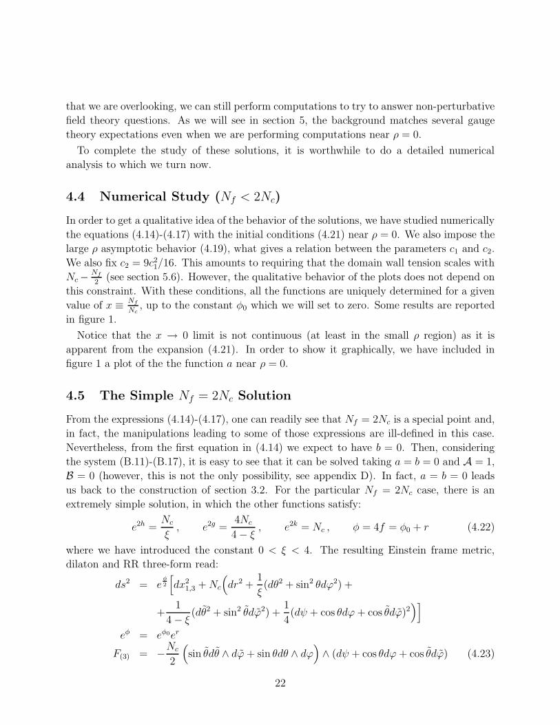
4.4 Numerical Study (Nf < 2Nc)

In order to get a qualitative idea of the behavior of the solutions, we have studied numerically

the equations (4.14)-(4.17) with the initial conditions (4.21) near ρ = 0. We also impose the

large ρ asymptotic behavior (4.19), what gives a relation between the parameters c1 and c2.

We also fix c2 = 9c21/16. This amounts to requiring that the domain wall tension scales with

Nc− Nf

2(see section 5.6). However, the qualitative behavior of the plots does not depend on

this constraint. With these conditions, all the functions are uniquely determined for a given

value of x ≡ Nf

Nc, up to the constant φ0 which we will set to zero. Some results are reported

in figure 1.

Notice that the x → 0 limit is not continuous (at least in the small ρ region) as it is

apparent from the expansion (4.21). In order to show it graphically, we have included in

figure 1 a plot of the the function a near ρ = 0.

4.5 The Simple Nf = 2Nc Solution

From the expressions (4.14)-(4.17), one can readily see that Nf = 2Nc is a special point and,

in fact, the manipulations leading to some of those expressions are ill-defined in this case.

Nevertheless, from the first equation in (4.14) we expect to have b = 0. Then, considering

the system (B.11)-(B.17), it is easy to see that it can be solved taking a = b = 0 and A = 1,

B = 0 (however, this is not the only possibility, see appendix D). In fact, a = b = 0 leads

us back to the construction of section 3.2. For the particular Nf = 2Nc case, there is an

extremely simple solution, in which the other functions satisfy:

e2h =Nc

ξ, e2g =

4Nc

4 − ξ, e2k = Nc , φ = 4f = φ0 + r (4.22)

where we have introduced the constant 0 < ξ < 4. The resulting Einstein frame metric,

dilaton and RR three-form read:

ds2 = eφ2

[

dx21,3 +Nc

(

dr2 +1

ξ(dθ2 + sin2 θdϕ2) +

+1

4 − ξ(dθ2 + sin2 θdϕ2) +

1

4(dψ + cos θdϕ+ cos θdϕ)2

)]

eφ = eφ0er

F(3) = −Nc

2

(

sin θdθ ∧ dϕ+ sin θdθ ∧ dϕ)

∧ (dψ + cos θdϕ+ cos θdϕ) (4.23)

22

1 2 3 4Ρ

0.2

0.4

0.6

0.8

1

ã2 k

0.5 1 1.5 2 2.5 3 3.5 4Ρ

2

4

6

8

10ã2 g

0.5 1 1.5 2 2.5 3 3.5 4Ρ

0.25

0.5

0.75

1

1.25

1.5

1.75

2ã2 h

0.5 1 1.5 2 2.5 3Ρ

0.2

0.4

0.6

0.8

1

1.2

1.4

Φ

0.5 1 1.5 2Ρ

0.2

0.4

0.6

0.8

1

a

0.1 0.2 0.3 0.4 0.5Ρ

0.8

0.825

0.85

0.875

0.9

0.925

0.95

0.975

a

Figure 1: Some functions of the flavored solutions for Nf = 0.5Nc (thin solid lines), Nf =1.2Nc (dashed lines), Nf = 1.6Nc (dotted lines). For comparison, we also plot (thick solidlines) the usual unflavored solution. The graphs are e2k, e2g, e2h, φ, a and a zoom of the plotfor a near ρ = 0. In the figures for a we have also plotted with a light solid line a = 1

cosh(2ρ).

We will discuss the gauge theory associated to this background in section 6.

4.5.1 A Flavored Black Hole

In section 4.3.2, we discussed the fact that the 0 < Nf < 2Nc solutions present a curvature

singularity, which is good according to the criterium of having bounded gtt. The Nf = 2Nc

case presents the same kind of singularity at r → −∞. However, the simplicity of this

metric allows us to check that this singularity also satisfies an alternative criterium, that

23

basically states that a gravity singularity is good if it can be smoothed out by turning on

some temperature in the dual field theory and thus finding a black hole solution [26]. So, in

order to construct the black hole, let us first make a change of variable,

r = 2 log z , (4.24)

and define:

F = 1 −(z0z

)4

(4.25)

Keeping the same dilaton and three-from but deforming the metric to:

ds2 = eφ02 z[

− Fdt2 + dx21 + dx2

2 + dx23 +Nc

( 4

z2F−1dz2 +

1

ξ(dθ2 + sin2 θdϕ2) +

+1

4 − ξ(dθ2 + sin2 θdϕ2) +

1

4(dψ + cos θdϕ+ cos θdϕ)2

)]

(4.26)

provides a regular solution of the Einstein equations (3.23), (3.24). As a technical comment,

notice that, due to the change in the metric, the expressions for T flavortt and T flavorrr get

multiplied, with respect to those in (3.27) by F and F−1 respectively. The rest of (3.27)

remains unchanged.

Let us stress that this solution has its own interest since it is, to our knowledge, the first

solution dual to a field theory in four dimensions with adjoints and fundamentals at finite

temperature8. We will explore some of the gauge theory aspects of this solution (4.26) in

section 6.

Finally, to close this section, we mention a numerical solution described in detail in ap-

pendix D. This solution for the case Nf = 2Nc, appears after a careful analysis of the BPS

eqs and has remarkable features. We comment more on it at the end of section 6.

5 Gauge Theory Aspects and Predictions of the Solu-

tion (Nf 6= 2Nc)

In this section we will study the family of gauge theories dual to the solution(s) we have

presented in the previous section. We will first try to give arguments towards a definite

lagrangian dual to the background (4.9)-(4.17) and then we will study different strongly-

coupled aspects of these field theories to support our proposal. These aspects include R-

symmetry breaking, pair creation and Wilson loops, instantons, Seiberg duality, domain

walls and asymptotic beta functions.

8In an interesting work [27], the addition of finite temperature to a three dimensional gauge theory withadjoint and fundamental fields was studied.

24

5.1 General Aspects of the Gauge Theory

Below we will present some arguments to motivate a lagrangian description for the field

theory dual to our backgrounds (4.9)-(4.17). We will argue that the dual field theory is

related in the IR to N = 1 SQCD plus a quartic superpotential for the quark superfields.

Some aspects related to the smearing of the flavor branes and to the six-dimensional little

string UV completion of the theory are not completely under control, and in particular we

could expect that some operator we are overlooking might still be present and slightly deform

the IR dynamics of the theory. Nonetheless we are confident that the result to which we

arrive is robust and we present many tests in the following, which support our interpretation.

Our argument starts by reminding the discussion in section 2.1, that the field theory dual

to the unflavored solution of [7] is six-dimensional N = 1 SU(Nc) SYM compactified on a

twisted two-sphere in such a way that the low-energy theory is four-dimensional and N = 1

supersymmetric. The spectrum of the corresponding U(1) theory is related to that of the

four-dimensional U(M) N = 1∗ theory, that is N = 4 SYM with equal masses for the adjoint

chiral multiplets, in its Higgs vacuum [20]. Let us briefly review the main features of this

four-dimensional theory before arguing how to extend this remarkable result to the large Nc

case. The superpotential of the N = 1∗ theory can be written (in N = 1 notations) as

W = TrU(M)

(

iΦ1[Φ2,Φ3] +µ

2

∑

i

Φ2i

)

(5.1)

and therefore the F-term equations of motion read

[Φi,Φj] = iµǫijkΦk (5.2)

It is immediate to recognize an su(2) algebra in this equation. This allows for non-trivial

solutions to (5.2) where the adjoint fields Φi are taken to be proportional to the generators

J(n)i of any irreducible representation of su(2). For any dimension n there is only one such

representation and therefore the classical vacua of this theory correspond to the partition of

M into positive integer numbers [28]

M∑

n=1

n kn = M (5.3)

where kn is the number of times the n-dimensional irreducible representation appears in the

expectation value of the adjoint fields. Any specific such vacuum has residual gauge group∏

n U(kn). To obtain a vacuum with gauge group U(1), one has to take kM = 1 and all other

kn’s to zero, whereas to obtain a vacuum which has exactly SU(Nc) residual gauge group,

one needs to start from SU(M) N = 1∗ with M an integer multiple of Nc, M = mNc, and

to take km = Nc in (5.3). The expectation values of the adjoint fields in this Higgs vacuum

25

satisfy the relation

Φ21 + Φ2

2 + Φ23 = µ2 M

2 − 1

4, (5.4)

that is they describe a (fuzzy) two-sphere.

In the particular case U(1), it was shown in [20] that the matching of the spectrum to

that of the compactified six-dimensional theory we started with, is exact in the M → ∞limit. Because of the ways the U(1) and the SU(Nc) vacua are built, it is natural to argue

that the results of [20, 21] extend to the more general SU(Nc) case, that is the spectrum

and lagrangian of the km = Nc Higgs vacuum of N = 1∗ is exactly the same as that of the

six-dimensional SU(Nc) SYM wrapped on a twisted two-sphere when m→ ∞.

Let us consider now the case we are interested in, that is the addition of flavors to the

compactified six-dimensional theory. When we add Nf flavor branes into the background,

we are effectively adding a set of massless chiral multiplets transforming in the fundamental

and anti-fundamental of the SU(Nc) gauge group. Let us call these multiplets Q = (S, q)

and Q = (S, q). These fields are massless because the flavor branes are at zero distance from

the color branes that generated the background.

A generic lagrangian for this new system could then be written as

L = Tr[

∫

d4θ(

Φ†KKe

V ΦKK +Q†eVQ+ Q†eV Q)

+

∫

d2θ(

W 2α + W

)

]

(5.5)

where W is a chiral superpotential describing the mass terms and self-interaction of the

adjoint Kaluza-Klein states, and their coupling to the fundamental fields. Because of the

argument above, we can think of the Kaluza Klein states as the three massive adjoint fields

of the N = 1∗ theory. The most natural way to couple the fundamental fields to an adjoint

state is mediated from the only allowed term in N = 2 SQCD, which is the one typically

appearing in intersecting branes setups. It reads

W = κ QΦQ (5.6)

with κ a coupling constant whose value will not affect our discussion. In a theory like the

N = 1∗ in a Higgs vacuum described above, if the fundamentals couple to a single adjoint

field through (5.6), the SU(2) global symmetry that rotates the three adjoints breaks down

to a U(1) subgroup. The term (5.6) breaks explicitly also the SU(Nf )×SU(Nf ) flavor group

to its diagonal SU(Nf ) subgroup.

The explicit flavor group breaking is exactly matched in our dual string picture by the

presence of flavor D5-branes alone, rather than of flavor D5 and anti-D5 branes. This

feature is in contrast with other models of theories with fundamental degrees of freedom

where the chiral symmetry breaking is spontaneous and flavors are added to the picture via

both D-branes and anti D-branes, which reconnect in the IR to account for the spontaneous

breaking [29]. Since in our case the breaking of the global symmetry is explicit rather than

spontaneous, we do not expect to find Goldstone bosons in the spectrum.

26

Regarding the breaking of the SU(2) to U(1), a little more care is required since the

smearing of the flavor branes restores the SU(2) symmetry in our model. Let us start,

therefore, from a different distribution of the flavor branes to try to understand what is

happening. We could smear the flavor branes on the (θ, ϕ) two-sphere, while putting all of

them on a single point on the (θ, ϕ) directions, for simplicity let us say at θ = 0. Since the

exact unflavored solution of [7] is invariant under an SU(2) acting on the ψ, θ and ϕ angles,

this new configuration breaks this SU(2) background isometry to U(1). We claim that this is

the configuration dual to the fundamental-adjoint coupling (5.6). From the field theory point

of view this would probably be the most natural brane configuration to consider, but as we

already mentioned above, finding a solution to the Einstein and flux equations for this less

symmetric configuration would probably turn out to be technically impossible. This is the

reason why we considered a smeared configuration for the flavor branes. Let us try, therefore,

to understand what this means in field theory terms. We know from (5.4) that the three

massive adjoint fields describe a two-sphere (in the limit M → ∞ it is a smooth sphere).

Therefore, we can take them to be parameterized by two angles (θ and ϕ), by the usual

projections over the coordinate planes of R3 of a two-sphere of radius R2 = µ2(M2 − 1)/4

centered at the origin. We will denote these adjoints parametrizing the S2(θ, ϕ) as Φ(i)

(θ,ϕ).

Then, we propose that the fundamental-adjoint coupling corresponding to our model is,

schematically:

W ∼ κ

∫

S2

dθ dϕ sin θ Q(

Φ(1)

(θ,ϕ)+ Φ

(2)

(θ,ϕ)+ Φ

(3)

(θ,ϕ)

)

Q (5.7)

Let us quickly go through now the low-energy effective lagrangian corresponding to the

superpotential (5.7). In general, if the parameter µ is much bigger than the scale of strong

coupling Λsqcd we can integrate out the KK fields from (5.5) to end up with an N = 1

SQCD-like theory that looks

L = Tr[

∫

d4θ(

Q†eVQ+ Q†eV Q)

+

∫

d2θW 2α + W ′

]

(5.8)

where the effective superpotential W ′ will depend on the way the adjoints couple to the

fundamentals and to themselves in (5.5). For our case (5.7), after integrating out the massive

KK fields, we might expect to obtain some combination of the quartic operators (5.6):

W ′ ∼ κ

µ(Tr(QQQQ) + (TrQQ)2) (5.9)

and possibly some more complicated operator due to the cubic coupling of the adjoint KK

fields.

Could we take the KK masses to be very large (µ → ∞), we would end up with pure

SQCD. Unfortunately, there is no known way to sensibly separate µ from Λsqcd without

27

requiring the full string dynamics9. In fact, one can expect that taking µ → ∞ requires

reducing the “external” space (that is topologically S2 × S3) to a stringy scale. In this

context, it is very suggestive that our construction has some similarity with the non-critical

string model of Klebanov and Maldacena [12], which, in fact, should be the limit of our

construction when continuously increasing µ→ ∞. Let us emphasize once again that, in the

process, the curvature of space-time reaches the string scale and therefore one cannot expect

to get reliable results from supergravity (although it has been shown that it is possible to

get some qualitative information from that kind of setups using a gravity action as a toy

model [12, 13, 16]).

We can now complete the comparison of the isometries of the field theory and of our

background. We have already analyzed the matching of the flavor symmetry and the SU(2)

Kaluza-Klein symmetry. The field theory at weak coupling also has a U(1)B×U(1)R symme-

try, where U(1)B is an exact baryonic symmetry, while U(1)R is the anomalous R-symmetry.

The unbroken baryonic symmetry could be associated with rotations along ϕ, whereas the

anomalous R-symmetry corresponds to shifts of the coordinate ψ. As we will analyze in

detail in section 5.4, the supergravity background reproduces faithfully the breaking pattern

U(1)R → Z2Nc−Nf→ Z2.

Finally, let us mention that in the special case Nf = 2Nc we can reasonably claim that

all the extra uncontrolled terms appearing along with (5.9) in the effective superpotential

W ′ can be turned off, giving on the string side our simple solution (4.23). As we show in

section 6, this background has very special features which we relate to the scale invariance

of the dual field theory. On the other hand, for Nf < 2Nc, we could not find a way on

the gravity side to turn off these extra terms, as the comparison between the solutions of

section 4.4 and of appendix D to the simple solution (4.23) seems to confirm. Nonetheless,

as all the rest of this section shows, the string dual perspective of many strong-coupling

effects, remarkably agrees with expectations from the field theory described by (5.8)-(5.9),

and allows therefore to make interesting predictions for its non-perturbative dynamics.

As a concluding remark, it would certainly prove very interesting to try to match with our

approach, the results of the careful analysis done in [32] on the vacuum structure of N = 2

SQCD with supersymmetry broken to N = 1 by a mass term for the adjoint superfield,

which is closely related to the theory (5.8), (5.9).

9This is the typical problem that afflicts all the supergravity duals to confining field theories. This will becleanly solved when a worldsheet CFT is found for these models lifting the limitation α′ → 0. Meanwhile,from a supergravity perspective, the KK modes can be disentangled form the gauge theory dynamics following[19, 30, 31].

28

5.2 Wilson Loop and Pair Creation

One natural question is what happens to the gauge theory Wilson loop, now that we have

massless flavors. In principle, as in QCD we should not observe an area law, but the SQCD-

string should elongate until its tension is equal to the mass of the lightest meson, and then

break. So, if we find that the (very massive) quarks that we introduce in the system feel each

other up to a maximal distance only, this will be indication that we are seeing a phenomenon

like pair creation10. In order to study this, we will follow a very careful treatment to compute

the Wilson loop in gravity duals [34] developed in [35] (for a good summary of the results, see

pages 19-25 in [36]). As usual, we propose that the Wilson loop for two non-dynamical quarks

(strings stretching up to ρ → ∞) separated a distance L in the gauge theory coordinates,

should be computed as the action of a fundamental string that is parametrized by t = τ ,

x1 = σ, ρ = ρ(σ) [34]. By solving the Nambu-Goto action, one obtains a one-parameter

family of solutions depending on an integration constant which we will define to be ρ0 (the

minimal ρ reached by the string). We convert to string frame the metric (4.9) and use (4.2)

and (4.5). Then, the length and energy (renormalized by subtracting the infinite masses of

the non-dynamical quarks) read:

L(ρ0) = 2

∫ ρ1

ρ0

ek(ρ)eφ(ρ0)

√e2φ(ρ) − e2φ(ρ0)

dρ ,

E(ρ0) =1

2πα′

[

2

∫ ρ1

ρ0

e2φ(ρ)+k(ρ)

√e2φ(ρ) − e2φ(ρ0)

dρ− 2

∫ ρ1

0

eφ(ρ)+k(ρ)dρ

]

(5.10)

where ρ1 is a cutoff related to the mass of the heavy quarks that can be taken to infinity

smoothly. These integrals can be performed numerically. In order to do so, we have to fix

the parameters c1 and c2 of the expansion (4.21) in order to give initial conditions for the

equations (4.15), (4.16). Imposing the large ρ asymptotic behavior (4.19) gives a relation

between them. Moreover, we also fix c2 = 9c21/16 so that the domain wall tension scales

with Nc − Nf

2(see section 5.6). However, this condition is not essential for the qualitative

behavior. The numerical result is reported in Figure 2. There is a finite value of ρ0, say

ρ∗0, for which the solution reaches a maximum Lmax (at this point, dLdρ0

= dEdρ0

= 0). There

is also a minimum value of the length Lmin = π√gsNcα′. Our interpretation is that Lmin is

related to the KK scale at which the UV completion sets in, and, therefore, the background

loses predictivity. For a range of Lmin < L < Lmax, there are two solutions of the Nambu-

Goto action. The physical one (the one of lower energy), corresponds to ρ0 > ρ∗0 which in

particular implies that the string never approaches ρ = 0 and therefore it does not approach

the curvature singularity.

As explained above, when one stretches a flux tube in a confining theory with dynamical

quarks, the tube must break at some finite length when there is enough energy to create

10In [33], screening due to backreacting flavors was found as a change in the slope of Regge trajectories.

29

3.4 3.6 3.8 4 4.2 4.4 4.6 4.8L

-10

10

20

E Nf=0.2 Nc

3.2 3.3 3.4 3.5 3.6 3.7 3.8L

-20

-10

10

20

E Nf=0.5 Nc

Figure 2: Energy vs. length of the Wilson loop forNf

Nc= 0.2 and

Nf

Nc= 0.5. Energies

are in units of eφ0√gsNc√α′ , whereas lengths are in units of

√gsNcα′ .There is a value of the

integration constant ρ0 for which the string reaches its maximum L and E. Longer stringsare not solutions of the Nambu-Goto action. We interpret it as string breaking due toquark-antiquark pair creation.

a light meson which screens the color charge. The geometry can reproduce this behavior

(the breaking happens at Lmax) because the backreaction of the flavors has been taken

into account. The graphs qualitatively match those found on the lattice in similar (non-

supersymmetric) setups [37]. Thus, our solution is showing that there is pair creation and

giving a prediction for the lightest meson in terms of the parameters of the model. The

fact that Lmin and Lmax are roughly of the same order reflects the known fact that, when

constructing the gravity dual of a confining theory, the KK scale and Λqcd are of the same

order and cannot be separated within a weakly curved framework.

The discussion above should be compared with what happens in unflavored backgrounds,

like (2.1)-(2.8), the KS background [6] or the ones we present in section 8, where there is no

possibility of extremizing the function L(ρ0). However, notice that the behavior found above

is very similar to the one observed in the paper [38] for a gravity dual of YM∗ without flavors.

Such a background, like ours, presents a good singularity in the IR and the authors of [33]

considered the Wilson loop behavior unphysical and related to the fact that the string wanted

actually to fall in the singularity. Nevertheless, there is an important difference between the

two models since gtt (and therefore the QCD string tension) never vanishes in our setup.

5.3 Instanton Action

Let us compute the action of an instanton in the field theory. We will propose that a gauge

theory instanton should be thought of as a euclidean D1-brane wrapping some contractible

two-cycle in the geometry (4.1). The action of the D1-brane is:

S = T1

∫

d2ze−φ√

detg + T1 i

∫

C(2) =8π2

g2sqcd

+ iθsqcd (5.11)

30

where we have compared with the action of the instanton in order to get an expression for

the four-dimensional gauge coupling and theta angle. Since dF(3) 6= 0, it is not possible to

define a two-form potential such that F(3) = dC(2). But if we consider the subspace given by

θ = θ, ϕ = 2π − ϕ (and take also large constant ρ) we can write, from (4.12):

F(3)eff =Nc

4(2 − x) sin θdθ ∧ dϕ ∧ dψ (5.12)

and therefore:

C(2)eff = (ψ − ψ0)Nc

4(2 − x) sin θdθ ∧ dϕ (5.13)

We now pick the two-cycle defined by [39] :

θ = θ, ϕ = 2π − ϕ, ψ = (2n+ 1)π (5.14)

So we can identify11:

θsqcd =1

2(2Nc −Nf )(ψ − ψ0), , (5.15)

4π2

g2sqcd

= e2h +e2g

4(a− 1)2 (5.16)

It is quite nice to see that the coupling constant satisfies the confining behavior we expect

for Nf < 2Nc. Indeed, plugging in the expansions for the functions near the origin (4.21),

we see that even though the solution is singular, this singularity is not causing problems and

the coupling grows at low energies. Conversely, in the UV, using the expansion in (4.19),

we observe that the coupling is asymptotically small. We will further discuss the quantities

written in (5.15), (5.16) in sections 5.4 and 5.5 respectively.

5.4 U(1)R Breaking

In the previous subsection, we have identified a contractible two-cycle on which we wrapped

a euclidean D1-brane that we identified as an instanton. Since this cycle contracts to zero

near the origin of the coordinates, the partition function for this euclidean brane should be

equal to one, up to a phase. For the original presentation of this argument see [40]. The

partition function of this instantonic string is

Z = (...) exp[i

2π

∫

Σ2

C(2)eff ] (5.17)

11We remind the reader that we have used that the tension of the D1-brane is T1 = 12πα′gs

and we are

using α′ = gs = 1 along our computations.

31

where Σ2 is the cycle (5.14) and (...) represents the Born-Infeld part of the action, see (5.11).

Under a shift in the R-symmetry ψ → ψ + 2ǫ (we write the factor of 2 since ψ ∈ [0, 4π) in

order to have ǫ ∈ [0, 2π)) we will have

Z → Z[0] exp[iǫ(2Nc −Nf)] (5.18)

so, asking for invariance of Z imposes that (this is equivalent to requiring that the θsqcddefined in (5.15) is unchanged modulo 2π under shifts of ψ):

ǫ =2κπ

2Nc −Nfκ = 1, ..., 2Nc −Nf (5.19)

So we see that quantum effects select a discrete subset Z2Nc−Nfout of the possible rotations

of the angle ψ associated with the R-symmetry, that is consequently broken according to

U(1)R → Z2Nc−Nf→ Z2, with the last step in the chain of breakings due to the fact that the

full background is only invariant under ψ → ψ+2π. This last step in breaking is understood

as the formation of a condensate, to which the functions a(ρ), b(ρ) should be dual to [41].

Notice that when Nf = 2Nc the breaking above does not happen and the U(1)R symmetry

preservation indicates a theory with higher invariance, in this case, scale invariance: the

U(1)R anomaly is in the same anomaly multiplet as the beta function so, when Nf = 2Nc

the coupling in (5.16) should not run. We study this point in more detail in section 6.

5.5 Beta Function

Let us start by summarizing the result of the wilsonian beta function for SQCD

βg = −g3sqcd

16π2(3Nc −Nf (1 − γ0)), (5.20)

where γ0 is the anomalous dimension of the quark (and anti-quark) superfields, while for the

coupling of the quartic superpotential we have

βh ∼ (1 + 2γ0). (5.21)

An approach to the calculation of the beta function of SYM from a gravity dual is presented

in [39]. Without entering into the many possible discussions about the validity of this

computation (more on this in section 8.8), let us just repeat the steps in [39] for our case.

The coupling is defined in (5.16) and we define the radius-energy relation near the UV of

the field theory (at large values of ρ) as

(Λ

µ)3 ∼ a(ρ) ∼ b(ρ) ∼ e−2φ (5.22)

32

where with the symbol ∼ above we mean that all these definitions, when taken at large values

of the radial coordinate, give the same result. The idea of the first two definitions is that

these functions should be dual to the gaugino condensate or other condensate as proposed

in [41]. On the other hand, one might consider that the exponential of the dilaton is related

to the strong coupling scale as proposed in [7, 42]. Considering only the large ρ expansion

of the coupling defined in (5.16) and the functions in (5.22), we have

4π2

g2sqcd

∼ Nc(1 − x

2)ρ+ ...., log

µ

Λ∼ 2

3ρ (5.23)

So, a straightforward computation leads us to

β =dgsqcdd log µ

Λ

= −3g3sqcd

32π2(2Nc −Nf ) + ... (5.24)

where the last equality should be understood as valid only in an expansion for large values

of ρ. This shows that in the regime described by the large ρ region of the background,

the anomalous dimension of the quark superfield is γ0 = −1/2 (and therefore βh = 0).

Once again, this computation should be severely criticized regarding the approximations and

assumptions that are done (see section 8 for a different sort of criticism to this approach),

but we just wanted to spell it here to show that the coefficient 2Nc − Nf appears. This

also reinforces the fact that for the case in which Nf = 2Nc something special is happening

(and we know the solution changes qualitatively for that case). It would be interesting to

understand what happens when Nf > 2Nc.

5.6 Domain Walls

The domain walls of N = 1 SYM associated to the IR spontaneous breaking of the R-

symmetry ZZ 2Nc→ ZZ 2 correspond to D5-branes wrapping the finite S3 at ρ = 0 [7]. Their

associated worldvolume κ-symmetry matrix is:

iΓx0x1x2123ǫ∗ = ǫ (5.25)

As pointed out in [43], this projection commutes with those in (B.4) if and only if A = 0, i.e,

when the brane is placed at ρ = 0. So from the brane point of view, one finds, consistently,

that these objects are one half BPS.

In the flavored theory we are dealing with, we have argued that there is a also a spontaneous

IR breaking ZZ 2Nc−Nf→ ZZ 2 and therefore one would also expect to have domain walls. It is

easy to see, using the expansion (4.21) and the expressions in appendix B that it is also true

in our flavored case that limρ→0 A = 0, so the same kind of embedding at ρ = 0 preserves

again half of the supersymmetry. Notice also that the action for the domain wall D5-brane

33

wrapping the three-cycle parameterized by θ, ϕ, ψ at constant ρ is:

ED5 ∝ T5 e2φ+2g+k ∝ (gsNc)

12Nc e

2φ02(2 − x)

√c2

3c1(1 + 2ρ2 + ...) (5.26)

and it has indeed a minimum at ρ = 0 (we have used eq (4.21) and restored the dependence on

gs). Also, despite e2g and e2k tend to infinity and zero respectively, the relevant combination

(5.26) goes to a constant at ρ = 0, rendering a finite tension for the domain wall (its precise

value would depend on the integration constants c1, c2 and could be used to fix them). Thus,

we would like to stress that, even if at ρ = 0 we are precisely on top of the curvature

singularity, it is appealing to find sensible results from these simple computations.

5.7 Seiberg Duality

A remarkable feature of many N = 1 gauge theories that include matter transforming in the

fundamental representation of the gauge group (or even in the bifundamental representation

for a quiver gauge theory) is Seiberg duality [44]. In its simplest form, this can be stated as

saying that an N = 1 SU(Nc) gauge theory with Nf quarks and an N = 1 SU(Nf − Nc)

gauge theory with Nf quarks and a gauge-singlet meson have the same IR physics. When

the theory contains a quartic superpotential for the fundamental fields, the duality is a bit

more complicated [45] but nonetheless it retains the same relations between the number of

colors and flavors of the two Seiberg-dual theories as in the simpler case.

In this section we will argue that Seiberg duality appears in our construction in a remark-

ably simple and elegant way: it corresponds to switching between two alternative ways of

writing the background12.

The central point on which the realization of Seiberg duality in our model is based, is that

the internal space of our background has S2 × S3 topology, but the choice to use either the

space spanned by the pair (θ, ϕ) or by (θ, ϕ) as the S2 base of the S3 is (at least at first

sight) arbitrary. In fact, let us take the metric and F(3) flux to be written as, from (4.9),

ds2 = eφ2

(

dx21,3 + dr2 + e2h(e2

1 + e22) +

e2g

4

(

(ω1 + a(r)e1)2 + (ω2 + a(r)e2)

2)

+e2k

4ω2

3

)

(5.27)

and from (4.3) and (4.11)

F(3) =Nc

4{−ω1 ∧ ω2 ∧ ω3 − b(r)(e1 ∧ ω2 − e2 ∧ ω1) ∧ ω3+

−b′(r)dr ∧ (e1 ∧ ω1 + e2 ∧ ω2) − (1 − x)e1 ∧ e2 ∧ ω3}(5.28)

12A first hint of what we will develop for the non-abelian background can be easily gained in the simplerabelian case by looking at the way the value of the integral of F(3) (3.18) changes when it is evaluated over

the 3-sphere (ψ, θ, ϕ) or (ψ, θ, ϕ).

34

where the functions φ, a, g, h and k are numerically evaluated in section 4.4, b is given

by (4.14)

b(ρ) = (2 − x)ρ

sinh 2ρ(5.29)

and for convenience we have defined the following 1-forms

e1 = dθ e1 = dθ

e2 = − sin θ dϕ e2 = − sin θ dϕ

ω1 = cosψ e1 − sinψ e2 ω1 = cosψ e1 − sinψ e2 (5.30)

ω2 = − sinψ e1 − cosψ e2 ω2 = − sinψ e1 − cosψ e2

ω3 = dψ + cos θ dϕ ω3 = dψ + cos θ dϕ

ω3 = ω3 + cos θ dϕ = ω3 + cos θ dϕ

We know that the number of colors of the dual theory can be evaluated by integrating the

three-form flux over the internal S3 spanned by the angles θ, ϕ, ψ, as in (3.4)

NcT5 =1

2κ(10)

∫

S3

F(3) (5.31)

whereas the number Nf of flavors in the gauge theory is determined by the failing of the

Bianchi identity for F(3), equation (4.10).

It is easy to show that the 1-forms we defined in (5.30) satisfy the following identities13

ω21 + ω2

2 = e21 + e

22 ω2

1 + ω22 = e

21 + e

22

e1 ω1 + e2 ω2 = ω1 e1 + ω2 e2

ω1 ∧ ω2 = −e1 ∧ e2 ω1 ∧ ω2 = −e1 ∧ e2 (5.32)

e1 ∧ ω2 − e2 ∧ ω1 = −(e1 ∧ ω2 − e2 ∧ ω1) e1 ∧ ω1 + e2 ∧ ω2 = −(e1 ∧ ω1 + e2 ∧ ω2)

We can use these expressions to rewrite the metric and F(3) in a new form. It is very

important to notice that even though these two quantities will look quite different from

above, what we do is only a rewriting of (5.27) and (5.28). For the metric we obtain then

ds2 = eφ2

(

dx21,3 + dr2 + e2h(e2

1 + e22) +

e2g

4

(

(ω1 + a(r)e1)2 + (ω2 + a(r)e2)

2)

+e2k

4ω2

3

)

(5.33)

and for the three-form flux

F(3) =Nc

4

{

−ω1 ∧ ω2 ∧ ω3 − b(r)(e1 ∧ ω2 − e2 ∧ ω1) ∧ ω3+

−b′(r)dr ∧ (e1 ∧ ω1 + e2 ∧ ω2) − (1 − x)e1 ∧ e2 ∧ ω3

}

(5.34)

13We thank Agostino Butti for bringing these identities to our attention while describing to us the real-ization of the SU(2) × SU(2) isometry of the baryonic branch backgrounds of [24].

35

where in (5.33) we have defined

e2h =e2g

4

(

1 − a2e2g

4e2h + a2e2g

)

e2g = 4e2h + a2e2g

a = ae2g

4e2h + a2e2g

(5.35)

and in (5.34) we have set

Nc = Nf −Nc x =x

x− 1b(r) =

b(r)

1 − x(5.36)

in order for the new expressions of the metric and the three-form flux to have again the

same apparent form as in the original versions (5.27) and (5.28). By using the definition of

x = Nf/Nc and the expression for Nc, it is immediate to show that Nf = Nf . In the same

way, it follows from (5.36) and (5.29) that

b(ρ) = (2 − x)ρ

sinh 2ρ(5.37)

that is, exactly the same form as in (5.29) with the new value of the Nf/Nc ratio.

Because of the way the metric looks now (5.33), it seems natural to identify as the three-

sphere of the internal manifold, the one spanned by θ, ϕ and ψ. Therefore evaluating the

integral of F(3) over this S3, we find that the number of colors of the field theory dual to the

background (5.33)-(5.34) is Nc = Nf −Nc, whereas the number of flavors is still Nf . This is

very interesting because this is exactly the way the rank of the gauge group changes under

Seiberg duality.

Let us now compare the geometries in the IR, where Seiberg duality tells us that the two

field theories are the same. By using the small ρ expansions of section 4.3, we can derive the

behavior of h, g and a near the origin

e2h = e2h − 4

3(2 − x)ρ4 + . . .

e2g = e2g +4

3(2 − x)ρ2 + . . .

a = a− 2c1ρ3 + . . .

(5.38)

and remarkably we see that the newly defined functions correspond to their original homonyms

up to the third term in the small ρ series expansions. This is the holographic dual of the

statement that the Seiberg pair theories have the same IR behavior.

This result might look a little puzzling at first sight: in (5.33) and (5.34) we have only

written in a different way the metric and three-form flux but at the same time claim that

36

the background written in this way corresponds to a different theory from the one that is

dual to the (same) original solution (5.27) and (5.28). We believe the right way to look at

this puzzle is in terms of the dictionary we use to translate the geometry data into field

theory predictions. So in a sense, we have two different dictionaries we can use on the same

background, corresponding to the two ways of identifying the S3 inside the internal space.

This is a remarkable result: just by rewriting the flavored background in a different form,

we can capture the most relevant features of Seiberg duality for theories with flavors. In

fact in a simple and elegant way we can reproduce the change in the rank of the color gauge

group while leaving the number of flavors untouched, and we can show that the IR dynamics

of the two theories is exactly the same thanks to (5.38). It would be very interesting to

study how information about the Seiberg-dual field theory is encoded into string theory in

this setup, and which predictions this allows us to make.

6 Features of the Nf = 2Nc Solution

We now discuss the gauge theory interpretation of the particularly simple Nf = 2Nc solution

(or x = 2 in the notation introduced above), presented in section 4.5, see eq. (4.23). For

this solution (and only for this one), the effective four-dimensional Yang-Mills coupling, see

(5.16), is constant (notice that the coupling is constant regardless of the cycle used to define

it)4π2

g2sqcd

= e2h +e2g

4(a− 1)2 = Nc

4

ξ(4 − ξ). (6.39)

It is also the only solution for which the U(1)R symmetry is preserved. There is not anoma-

lous UV breaking (we can apply the discussion of section 5.4, eq (5.18)), while there is not

spontaneous IR breaking since a = b = 0. We would therefore not expect to have domain

walls and this is in fact the case since its tension as defined in (5.26) would vanish (e2φ → 0

when r → −∞). We think that these two features are signaling an IR conformal fixed point

in the effective four-dimensional theory.

That this happens only for Nf = 2Nc is in precise agreement with the field theory in-

terpretation of section 5.1. Notice that, unlike in pure N = 1 SQCD, there should not

be a conformal window for Nf ≤ 2Nc. In fact, having an IR effective quartic superpo-

tential for the quarks (5.9) fixes their R-charge to 12. The NSVZ beta-function, which can

be written in terms of the (IR) R-charges of the fields can consequently only vanish when

Nf = 2Nc. This can also be seen using the wilsonian beta-functions for the gauge coupling

βg ∼ (3Nc−Nf (1−γ0)) and the quartic coupling βh ∼ 1+2γ0 which vanish simultaneously if

and only if γ0 = −12

and Nf = 2Nc (γ0 is the anomalous dimension of the quark superfield).

Nevertheless, we cannot claim that the solution (4.23) is a faithful dual to a conformal

four-dimensional theory. Since there is no AdS5 space, the conformal group SO(2, 4) does

37

not show up in the gravity side and also there is no superconformal enhancement of the

supersymmetry. We believe that the explanation resides on the fact that we start with

a six-dimensional theory living on the D5-branes compactified with a twist on an S2 and

then add flavor branes. The four-dimensional theory never completely decouples from the

Kaluza-Klein degrees of freedom and this spoils the would-be conformal symmetry. Indeed,

even though the parameters and couplings might be tuned so that the massless modes are

in a “conformal phase”, the KK modes spoil this symmetry and the background reflects it

by not allowing an AdS5 to appear. To add to this interpretation we can, for instance, make

a dilatation of the four dimensional spacetime xi → λxi, that can be compensated (we take

string frame) by a shift r → r−2 log λ, which should be regarded as a rescaling of the energy

scale (see (5.22)). This is not an isometry of the metric since the internal space gets rescaled,

thus rescaling the KK scale. However, we find appealing that the geometry is not deformed

in any other way, since the functions h, g, k, a do not depend on r. Notice that this happens

only for this simple Nf = 2Nc solution.

In any case, one could not expect to find a weakly curved AdS5 since this would imply that

the coefficients of the conformal anomaly are equal a = c at leading order in Nc [46]. Since

our theory has Nf ∼ Nc, one has a 6= c at leading order [47], ruling out the possibility of

having a faithful supergravity dual. Nevertheless, we think it is very nice that some features

can be matched in this setup.

Finally, let us conjecture on the gauge theory meaning of the parameter ξ. N = 1

SQCD with Nf = 2Nc and a quartic superpotential has a one complex-dimensional family

of marginal deformations in the two complex-dimensional parameter space of the gauge

coupling and of the coupling of the quartic term (see [45]). The parameter ξ changes the

volume of the spheres (4.22) so it is natural to think that it would change the masses of the

adjoints coming from the KK modes and, indeed, modify the value of the coupling at the

“conformal fixed point” (6.39). Thus, it may be a parameter signaling this conformal line.

Let us see this more precisely. In this geometry, we could define couplings (not necessarily

the SQCD coupling in (6.39)), to be proportional to the inverse volume of two-cycles

1

g42∼ V olΣ2

g26

. (6.40)

Here g26 = α′gsN is the coupling of the little string theory. So, different definitions would

imply the choice of different two-cycles in the geometry, like

1

g2=V ol S2(θ, ϕ)

g26

,1

g2=V ol S2(θ, ϕ)

g26

,1

g2sqcd

=V ol S2(θ, θ, ϕ, ϕ)

g26

(6.41)

Let us be more precise and define the cycles above. The first two cycles are given by the

effective geometry obtained from (4.23) when imposing that all the coordinates are constant

except (θ, ϕ), or (θ, ϕ) in the case of S2(θ, ϕ) and S2(θ, ϕ) respectively. The last cycle is

defined like in (5.14) and gives the coupling in (6.39).

38

So, computing these “couplings” one gets

1

g2Nc∼ 1√

ξE[π,

ξ − 4

ξ]

1

g2Nc∼ 1√

4 − ξE[π,

ξ

ξ − 4]

1

g2sqcdNc

∼ 4

ξ(4 − ξ)(6.42)

Where E[π, k] is the second kind Elliptic function. Now, let us observe something quite

nice. If we interchange the cycles S2(θ, ϕ) ↔ S2(θ, ϕ), this is equivalent to the interchange

ξ ↔ (4 − ξ), or g ↔ g. The Seiberg-like duality defined in section 5.7 does precisely this

job. So, we have a line of fixed points, parametrized by ξ (solutions where the two-spheres

have constant radius), which is reflected under Seiberg duality. This is what is known to

happen in a field theory like the one discussed in section 5, that is N = 1 SQCD plus a

quartic potential, when the theory is at its conformal point (Nf = 2Nc, and the anomalous

dimension of the quark superfields is γ0 = −12). For a review of these results, see Strassler’s

beautiful lecture notes [45]. Indeed, following [45], we can see that the line of fixed points

has a self-dual point (under Seiberg duality), that in our case is ξ = 2. Then the duality, in

our case the interchange ξ ↔ (4 − ξ) or the interchange of two cycles, interchanges points

on the fixed line that lie on different sides of the self-dual point. We can see that this is

happening in eqs. (6.42), for a holomorphic coupling that should be a combination of gsqcdand the quartic coupling.

This suggests that as for the coupling (6.39), it might be possible to find another two-cycle

whose volume is inversely proportional to the quartic coupling. This is a very nice check

that points to the consistency of our approach and interpretation.

Finally, we would like to stress two very interesting facts. First, let us compute the Wilson

loop (see section 5.2, eq. (5.10)) for this particular case. It can be seen that for any value

of ρ0, one obtains that the quark antiquark pair has energy Eqq = 0 and that the separation

of the pair is always L = π√Ncgsα′. Following the interpretation of section 5.2, below

this length this computation is unphysical due to the UV completion. For L > π√Ncgsα′,

the configuration in which the qq are joined by a string is never preferred to having two

independent particles (notice that in this case, the QCD string tension vanishes gtt(r =

−∞) = 0). We interpret this observation as the existence of total screening, the “mesons”

have zero energy, in agreement with the fact that this theory does not dynamically generate

a scale.

The second observation concerns the black hole solution in (4.26). We can compute the

viscosity of the dual quark-gluon plasma following the approach developed in [48]. Since our

background (4.26) satisfies the hypothesis of the theorem in [49], we can see that the relation

between the shear viscosity and the temperature is of the predicted form D = 14πT

. It may

39

be interesting to study other hydrodynamical quantities using the dual solution (4.26). This

is a very simple background dual to a field theory with adjoints, fundamentals and at finite

temperature.

Finally, to close this section, we would like to call the reader’s attention to the solution

presented in appendix D. There we described a numerical solution for the case Nf = 2Nc,

that appears after a careful analysis of the BPS eqs. Interesting features of this solution are

that it has a behavior similar to the flavored case (with Nf 6= 2Nc), asymptotes in the UV to

the simple solution presented in eq. (4.23) and the fact that the solution is Seiberg-duality

invariant. We do not know how to interpret this new solution from a dual field theory

viewpoint. It seems to behave as a flow from a fixed point where a relevant operator is being

inserted, breaks “conformality” and goes down to an IR theory similar to the one described

by the solutions with Nf < 2Nc. We leave this interesting problem for future study.

7 An Alternative Approach: Flavors and Fluxes

As we have seen in section 4.2, the addition of many flavor branes to the MN background

is encoded in the non-closure of the three-form RR flux F(3). When the flavor branes are

smeared over their transverse directions, the failing of the Bianchi identity is proportional

to the volume form of the transverse S2 × S2

dF3 =Nf

4sin θ sin θ dθ ∧ dϕ ∧ dθ ∧ dϕ. (7.1)

In sections 3 and 4 we shown that this effect gives rise to a background which has a uniform

distribution of F(3) charge along the two two-spheres. As we have shown in the preceding

sections this procedure works very nicely and gives rise to a remarkable matching between

gauge theory expectations and string predictions.

Nonetheless, we think it could also be very interesting to approach the same problem

from a complementary approach. In this section we sketch the general idea and some basic

features of this possible new scenario, but setting up and solving the whole problem would

require a much deeper development and thorough discussion, which we leave as a possibility

for the future.

In this new approach, the failing of the Bianchi identity for the three-form F(3) is achieved

through non-trivial fluxes only. Indeed, we know from supergravity that the presence of an

NS three-form background deforms the definition of the field strengths of the RR fluxes. Let

us suppose to turn on some axion C(0) and NS flux H = dB(2), then the field strength F(3)

is defined by

F3 = dC(2) − C(0)H (7.2)

and we see that if the axion is non-constant we can have a non-trivial Bianchi identity for

40

F(3)

dF3 = −dC(0) ∧H = −F(1) ∧H (7.3)

Notice that in this case the decomposition of F(3) in an exact and non-exact part is natural,

and therefore the definition of C(2) is unambiguous (up to gauge transformations, obviously).

In the preceding sections we have always assumed that the susy transformations of the

flavored background are exactly the same as those of the MN solution [7, 15]. This is due

to the fact that we are adding to the MN solution an (infinite) set of BPS branes, which

by definition preserve the same supersymmetries as the original background. But when

we look at the flavoring of the background from the flux side, this could fail, and in fact,

this is what one usually expects when turning on new fluxes in a background. The only

condition we think it is still sensible to impose, is that the background can accommodate

supersymmetrically embedded branes.

Regarding the geometrical properties of the six-dimensional internal manifold. There are

two possibilities to build backgrounds with fluxes that preserve four-dimensional N = 1

supersymmetry: SU(3)-structure manifolds [50] and a particular class of SU(2)-structure

manifolds [51]. The unflavored MN background the internal manifold has SU(3)-structure

[50] and since we can most likely think of the flavored background as a deformation of the

MN solution, it seems reasonable to assume that its internal part is an SU(3)-structure

manifold as well.

Starting from these two assumptions, we can write the spinor ansatz for the supersymmetry

transformations. As usual for solutions with four-dimensional Lorentz invariance, we split

the IIB ten-dimensional spinors in their four-dimensional and internal six-dimensional parts

ǫ1 = ζ+ ⊗ η1+ + ζ− ⊗ η1

−

ǫ2 = ζ+ ⊗ η2+ + ζ− ⊗ η2

−(7.4)

where η1 and η2 are spinors of the internal manifold. Notice that ηi− = (ηi+)∗. Since SU(3)-

structures allow only for one globally-defined spinor η, we need to take η1 and η2 to be

proportional

η1+ = aη+ η2

+ = bη+ (7.5)

A necessary condition to have consistent supersymmetric embeddings of branes in an

SU(3)-structure manifold, is that the two spinors η1 and η2 have the same norm, ‖η1‖2 =

‖η2‖2 [52], which requires that the functions a and b in (7.5) satisfy

a

b= eiφ

a

b∗ = eiτ (7.6)

with φ and τ real functions of the internal coordinates. For the smeared configuration we

consider in this paper, symmetry imposes that they only depend on the radius of the internal

41

manifold. Notice that the spinor η is defined up to a phase, and therefore τ in (7.6) can be

arbitrarily gauge fixed by this symmetry [50]. On the contrary φ does not depend on the

gauge choice.

Instead of a and b we can define α and β

α = a + ib β = a − ib (7.7)

in such a way that when we define ǫ = ǫ1 + iǫ2, we get

ǫ = α ζ+ ⊗ η+ + β ζ− ⊗ η−

ǫ∗ = β ζ+ ⊗ η+ + α ζ− ⊗ η−(7.8)

In terms of α and β the first condition in (7.6) reads

α

β= −i cot

φ

2(7.9)

At this point, one should write a smart ansatz for the metric and background fluxes, and

then the SU(3)-structure techniques developed in [50, 53] would allow to derive first order

differential equations describing the solution. This is beyond the scope of the present work.

8 The Unflavored Case Nf = 0: Deformed Solutions

This section might be read almost independently of the rest of the paper and addresses the

problem of finding gravity duals to different UV completions to N = 1 SYM from the one

described in section 2. Concretely, we will deal with the setup presented in section 4.1.

These solutions have appeared, in the context of this work, because in the procedure we

devised to add flavors, we first deformed the original (unflavored) background (2.1)-(2.8),

see the details in section 4. As explained in section 4.1, these backgrounds are an interesting

subcase of the ansatz studied in [24].

Below, we will study a little more the interesting solutions of the unflavored system (4.1)-

(4.8). In section 8.1, we describe the backgrounds arising from the study of these equations

and in sections 8.2-8.8 we discuss their gauge theory interpretation.

8.1 Description of the Solutions

Equations (4.6) have a one-parameter family of regular solutions. In fact, for small values

of the radial coordinate, we find a very well controlled expansion in terms of a parameter µ

taking values in the interval (−2,−2/3]:

a(ρ) = 1 + µρ2 + ..., e2k = Nc

(

4

6 + 3µ− 20 + 36µ+ 9µ2

15(2 + µ)ρ2 + ....

)

. (8.1)

42

By inserting it in (4.7), (4.8) we find, for the other functions:

e2g = Nc4

6 + 3µ+ ..., e2h = Nc

4ρ2

6 + 3µ+ ..., e2f−2f0 = 1 +

(2 + µ)2

8ρ2 + .... (8.2)

In the case in which the parameter µ = −2/3 we reobtain the known solution (2.1)-(2.8),

that is:

a =2ρ

sinh 2ρ, e2k = Nc (8.3)

and in the case µ = −2 (and Nc = 0) we get four-dimensional Minkowski times the deformed

conifold (see appendix C). For ρ→ ∞ (except in the particular µ = −23

case), the solutions

asymptote to the deformed conifold metric (for details, see appendix C), i.e very far away

from the branes their effect becomes negligible and the background asymptotes to a Ricci

flat geometry.

In the figure 3 we present numerical plots of several of the functions defining the geometry

for different values of µ. Notice in particular that, unlike the usual solution (2.1)-(2.8), here

the dilaton does not diverge14.

8.2 Gauge Theory Analysis

All the deformed solutions presented in section 8.1 are non-singular duals to field theories

with field content being a non-abelian gauge field, a Majorana fermion and a set of massive

adjoint scalar multiplets. These field theories in principle confine since the warp factor in

the metric (4.1) goes to a constant value near ρ = 0. This will be analyzed in more detail in

section 8.7. Regarding the string theory picture, this is a compactification of Nc D5-branes

on a two-sphere, that preserves N = 1 SUSY. As studied in many places, and recently

reviewed in detail in [20], this leads to a field theory whose lagrangian is the one of N = 1

SYM coupled to a set of massive scalar multiplets. We will assume this picture below, and

will argue that the dynamics of the massive modes is related to the parameter that labels

the family of solutions.

Contrary to what one might think, this is not the “brane side” of the solution (2.1) (for

the case of D6-branes this “brane side” solution was found in [54]). If these new solutions

were the “brane-side”, one should see a resolved conifold and the metric structure that

characterizes the D5-branes, near the origin of the space. One might want to interpret this

new solution as the “non-near-horizon” version of the solution of D5-branes wrapping a two-

cycle inside the conifold. This must be at least partially correct, since at ρ→ ∞ one goes to

Ricci flat geometry and the effect of the fluxes disappears (notice also that a metric like (4.1)

14A usual criticism to solutions like (2.1)-(2.8) is that since the dilaton diverges for large values of theradial coordinate, one must S-dualize and we should be dealing with NS5 branes, hence, the UV completionis a little string theory, which is an unconventional completion for a field theory.

43

1 2 3 4Ρ

0.2

0.4

0.6

0.8

1

a

0.5 1 1.5 2 2.5 3 3.5 4Ρ

5

10

15

20

25ã2 k

1 2 3 4 5Ρ

0.7

0.75

0.8

0.85

0.9

0.95

ã2 k-2 g

0.5 1 1.5 2 2.5 3 3.5 4Ρ

5

10

15

20

25ã2 h

0.5 1 1.5 2 2.5 3 3.5 4Ρ

0.5

1

1.5

2

2.5

3

3.5ãΦ

Figure 3: We plot the different functions for different values of the parameter µ. The thicksolid line corresponds to µ = −2

3(the usual MN case), the solid thin lines correspond,

respectively, to µ = −.68,−1,−1.5 and the dashed line is a deformed conifold.

cannot be obtained by uplifting from 7d gauged sugra in the same way as (2.1)). However,

it cannot be the whole story since, as we will see, the IR physics is also modified within the

family of solutions.

The proposal we want to put forward is that different members of this family (that can be

thought of as different values of µ in the window (−2,−2/3]) differ in the superpotential that

affects the dynamics and masses of the KK modes. At the same time, it is also possible that

different members of this family differ in VEV’s for some operator. Then, the UV completion

of the theory changes, modifying the large ρ behavior of the background (this is in analogy

with turning on an irrelevant operator in AdS5 × S5). But this change in the UV dynamics

44

also alters the infrared (in analogy with what would be a dangerously irrelevant operator).

Indeed, we know that all these infinite solutions preserve N = 1 SUSY by virtue of a

twisting procedure in the gauge theory. It should be quite interesting to analyze how the

developments in [20, 21] apply to this new set of configurations. It is also interesting to notice

that any expansion that starts out of the window (−2,−2/3] for the parameter µ mentioned

above generates pathological solutions. This suggests that the dynamics of the KK modes is

such that it shows some instability or similar sick behavior for solutions that are outside this

window (as the supergravity solution becomes singular) 15. Besides, we stress that the values

µ = −2, µ = −2/3 correspond to conifolds with maximal and zero deformation parameter.

So, from the gravity side the existence of this window is clear, see appendix C.

A first check of our proposal comes from constructing new backgrounds doing solution-

generating transformations on these µ-family of solutions, that have a U(1)×U(1) isometry.

These isometries are global symmetries of the KK part of the spectrum, hence, constructing a

new background by SL(3, R) transformations based on those U(1)’s (following, for example,

the techniques developed in [55]), will only affect the dynamics of the KK modes. This

idea was proposed in [19, 30] to be the way to distinguish between a pure SYM effect

and the dynamics of the KK modes influencing some observable. When we perform the

transformation on this family of backgrounds (we will not report here the formulas, since

they are quite lengthy), we observe a mixing between the parameter of deformation γ and

the parameter µ (changing the dynamics of the KK modes).

In the following, we will study a sample of gauge theory observables that range from the

possible existence of massless axionic glueballs, k-string tensions, annulons and PP-waves

spectrum, Wilson loops and beta function. Technical details can be found in appendix E.

These examples will support the validity of the proposal that we have made above.

8.3 Axionic Massless Glueballs

In the paper [56], the authors studied the possibility of finding a massless glueball in the

exact solution (2.1)-(2.8). They found that this glueball was not normalizable, which led

them not to consider it to be a physical excitation. This is in contrast to what happens for

the Klebanov-Strassler solution or a non-supersymmetric deformation of it in which there

are, in fact, physical massless glueballs [56, 57].

In the exact (2.1)-(2.8) solution (µ = −23), the dilaton diverges at large values of the radial

coordinate and this is the root of the non-normalizability of this mode. In this new set of

solutions, we have that for µ 6= −2/3 the dilaton is bounded at infinity, see figure 3. It is

natural, therefore, to wonder whether this family of solutions might have a massless glueball.

Let us analyze this in some detail. In principle, we do not expect this massless glueball to

15One might speculate with the existence of a potential term in the KK lagrangian of the form (Φ denotesa generic KK mode) V = µ2/2Φ2 − (µ+ 2)(µ+ 2/3)Φ2n + ... that captures this behavior.

45

exist, since there is not in this model any apparent U(1)B symmetry that is spontaneously

broken, leading to a massless supermultiplet of composites.

In the paper [58] the fluctuated eqs of motion were studied in detail. Let us assume that

the background fields vary according to

gµν → gµν + ǫhµν , φ→ φ+ ǫδφ, Fµνρ → Fµνρ + ǫδFµνρ (8.4)

So, keeping only linear order in the parameter ǫ, we get eqs for the fluctuated fields that we

report in detail in appendix E. One can easily see that a solution to these eqs is the one

found by the authors of [56]

δF3 = ∗4da, hµν = δφ = 0; F3.δF3 = 0 (8.5)

Once again, the point in the paper [56], is that this fluctuation, due to the diverging dilaton

is not normalizable, so they reject the excitation as a physical state. We might wonder what

will happen now that we have a new family of solutions with a bounded dilaton. The norm

of the fluctuation is

|δF3|2 = (∗4da)2

∫ ∞

0

dre2k+2g+2h+5φ (8.6)

In this case the dilaton does not diverge, but the functions g, h, k are unbounded making again

the mode under consideration not normalizable. Even in this family of solutions, therefore,

we do not seem to have this massless glueball. There might be another combination of fields

that could play that role, but this does not seem likely, due to the fact that this family

of theories (if they differ from (2.1)-(2.8) in the masses and dynamics for the KK-modes

and possibly condensates) should not have a U(1) symmetry that is spontaneously broken

leading to a massless excitation.

8.4 Confining k-Strings

One very interesting problem in SU(N)-QCD and similar theories is the study of flux tubes

induced by color sources in higher representations. If the source has k fundamental indexes,

the flux tube is called the k-string. The law for the tensions of these k-strings has been

subject of interest, from the lattice viewpoint and also from a more formal side.

In the very nice paper [59], Herzog and Klebanov tackled this problem using AdS/CFT-like

dualities for confining theories. They considered a confining string (connecting quarks in the

antisymmetric representation) as a D3-brane wrapping a cycle near the IR of the geometry.

They found the tensions of these strings. Let us briefly summarize their approach and apply

it to our cases of interest. This can be done easily with the expansion written in (8.1)-(8.2),

since we have to look at the geometry near ρ = 0. It is easy to see that our geometry (after

the choice of the cycle θ = θ, ϕ = 2π− ϕ, ψ and a rescaling ψ → ψ/2) turns exactly into the

46

geometry in eq.(12) of [59]. So, near ρ = 0 the metric induced on these D3-branes that wrap

the cycle above and extend in (t, x) forming a confining string, reads

ds2 = e2f0[

dx21,1 + e2k(0)

(

dψ2 + cos2 ψ(dθ2 + sin2 θdϕ2))

]

. (8.7)

Following the approach of Herzog and Klebanov, we can compute the tension of the q-

confining string as the tension of a D3-brane wrapping the finite three-cycle above

T ∼[

b2 sin4 ψ + (ψ − sin 2ψ

2− πq

Nc)2]1/2

. (8.8)

The coefficient is b = e2k(0)

Nc= 4

6+3µ. Only for µ = −2/3, that is for the exact solution (8.3),

we have b = 1. It is precisely this coefficient the one that propagates into formulas (12)-(18)

of [59]. Then, when minimizing the action of this confining string, our formulas will be

exactly like the ones in [59]. The tension of the confining string is minimal when

ψ =1 − b2

2sinψ +

πq

Nc, Tq = b sinψ

√

1 + (b2 − 1) cos2 ψ (8.9)

The law that is conjectured to work for N = 1 SYM (see for example [60]) is

TkT ′k

=sin(πk/Nc)

sin(πk′/Nc)(8.10)

whereas the string tension in this family of models is not obeying a sine law, and only for

the exact solution (µ = −2/3) this behavior is reproduced. It is interesting to notice that

observables like this seem to diverge for µ = −2, but we know that this point is out of our

family.

We mentioned above that we could interpret the parameter µ as different masses, and

most likely also different parameters in the superpotential, for the KK modes. This matches

nicely with the findings of the paper [61]. The authors there have pointed out that if one

considers N = 1 SYM as broken N = 2 SYM, the sine law is not universal. The set of

models we have resembles quite much these N = 2 → N = 1 models (it is a little more

subtle since we have a twisting). In the analysis done in [59] for the Klebanov-Strassler (KS)

model, it was found that confining strings there do not present a sine law behavior. In this

aspect, the family of deformed solutions we are studying, behaves like the KS solution.

8.5 Rotating Strings

We will study rotating strings in the same spirit as advocated by Gubser, Klebanov and

Polyakov in the paper [62]. These rotating strings should be dual to large-operators in the

gauge theory (composed of a large number of adjoint fields). We will see that these strings

47

display characteristic energy-angular momentum relations and sample (for short strings) the

different dynamics of the KK modes, that is, they depend on the particular value of µ. There

are a number of solutions already found in [63, 31] that show this behavior. So, consider for

example a string that rotates on S2 and is stretched in the radial direction parametrized by

t = κτ, ϕ = ωτ, θ =π

2, ρ = ρ(σ). (8.11)

After writing the Nambu-Goto action, the energy and angular momentum can be computed

(for a string that stretches from the origin to a position ρ0) one gets [63, 31]

E ∼∫ ρ0

0

e2φ+2k

√

e2φ+2k(κ2 − ω2(e2h + e2g

4a2))

J ∼∫ ρ0

0

e2φ+2k(e2h + e2g

4a2)

√

e2φ+2k(κ2 − ω2(e2h + e2g

4a2))

(8.12)

By doing an expansion near ρ0 ∼ 0, that is by considering short strings, it is easy to see that

the dispersion relations for this string depends on the parameter µ. This means that the

operator dual to this string configuration contains a gauge invariant combination of fields,

including the KK fields discussed above. In other words, these operators will have different

energy-angular momentum relations depending on the member of the family of solutions we

consider.

Now, we would like to study string configurations whose energy and angular momentum

expressions do not depend on the µ parameter. The latter are more interesting than the

solutions discussed above, since they should be dual to pure gauge theory operators made

out of Aµ, λ and derivatives; so we will be more detailed. For this, we consider a configuration

for a bosonic string that rotates on “the gauge theory space” and on an internal direction

(chosen so that it will give the string some R-charge) and also stretches along the radial

direction. We consider the ansatz (see appendix E for details)16:

t = κτ , x = R(σ) cos(ω1τ) , y = R(σ) sin(ω1τ) ,

ρ = ρ(σ) , ψ = 2ω2τ (8.13)

Let us take a look at some particularly interesting solutions.

Rotating folded closed string

Let us consider constant ρ. Then, one has to take ρ = ω2 = 0 (notice that, at ρ = 0, we

have ∂ρk = ∂ρφ = 0) and:

R =1

ω1

cosω1σ (8.14)

16See also [64] for the discussion of a similar configuration in the backgrounds of [7, 65].

48

This is dual to a high spin glueball. Notice that the slope of the Regge trajectory will depend

on the tension of the string at the bottom of the geometry and therefore on eφ0 .

Pointlike strings rotating in ψ

Consider:

R = const ρ = const (8.15)

Then, we need ω1 = 0 and:

∂ρk = 0 ⇒ ρ = 0

e2kω22 = 1 (8.16)

These strings are dual to (long) R-charged operators .

It is interesting to notice that when computing observables for these strings, like energy

and angular momentum (R-charges), they do not depend on the parameter µ hence, they

are the same for different members of the family. This can be interpreted as an indication17

that these strings are a purely gauge theory effect and are dual to (large) operators that

are gauge invariant combinations of Aµ, λ. On the contrary, moving strings like the ones

considered in (8.11)-(8.12) (originally found in [63, 31]), show dependence on the µ parameter

when computed in these new backgrounds. This is because they are dual to large operators

containing KK modes, as established in [31] (following the proposal of [19]). It would be

interesting to recompute our solutions above in the deformed background proposed in [19].

8.6 Penrose Limits and PP-waves

This subsection is constructed on the work done in the very good paper [66]. Let us summa-

rize their findings. They studied a Penrose limit of the background (2.1)-(2.8) on a geodesic

that is mostly localized near ρ = 0. The limit gives a PP-wave geometry on which the string

theory can be quantized. The authors of [66] associated this geodesic on the string side with

an operator on the gravity side that looks like a large chain composed of KK modes, that

they called annulon. The spectrum of excitations of the annulon was put in correspondence

with the spectrum of the string on the PP-wave geometry [66]. We will follow their approach

and take the same Penrose limit on our one-parameter family of solutions. The details of the

computation are spelled out in appendix E. After following the approach in [66] adapted to

the present case, we get a plane wave background that looks

e−2k(0)−φ(0)/2L2ds2 = −2dx+dx− + d~x23 + d~y2

2 + dz2 +1

4d~v2

2 − (~v2

2

4+µ2

4~y2

2)dφ2+,

F3 = (2dv1 ∧ dv2 +µ

2dz1 ∧ dz2) ∧ dx+. (8.17)

17Notice that most probably µ-independence is a necessary but not sufficient condition to ensure that theoperator does not contain KK modes.

49

So, we see that we have four massless directions (~x3, z) and four massive ones; ~v2 with mass18

m2 = 1 and ~y2 with m2 = µ2/4. The excitations of this PP-wave are dual to operators

composed out of KK modes and one can clearly see that the parameter µ is related to

the mass of the KK modes. As we mentioned before, it may be the case that µ is also

influencing the dynamics of the KK’s or condensates, but this is erased in the Penrose limit

and we only see the effect in the masses. So, following the treatment in [66], we can compute

the spectrum for strings on this family of pp-wave backgrounds and put the dynamics of this

string in correspondence with the dynamics of the family of annulons.

8.7 Wilson Loop

We would like to analyze here a subtle point related to Wilson loops. We will follow the

treatment developed in [35] and carefully revised in [36]. We will consider a probe brane that

is wrapping the same 2-cycle as the branes that originate the geometry, but this probe brane

is very far away from the origin (this probe was proven to be SUSY preserving in [15]). This

leads to very massive fields that we associate with quarks, and we compute the expectation

value of the Wilson loop as

< W >∼ eSNG (8.18)

where SNG is the Nambu-Goto action for a string in the background (4.1). After choosing a

configuration for a string that extends in the coordinates x, ρ, t and is parametrized by the

worldsheet coordinates σ, τ according to x = σ, ρ = ρ(σ), t = τ , the NG action will read

SNG =1

2πα′

∫

dσ√

|gxxgtt| + |gttgρρ|ρ′2 =1

2πα′

∫

dσ√

F 2(σ) +G2(σ)ρ′2 (8.19)

Notice that this action implies the existence of a conserved quantity, that we associate with

F (ρ0), where ρ0 is the point of maximal proximity of the probe string to the origin of space

ρ = 0. The separation of the two very heavy quarks is given by L = 2F (ρ0)∫ ρ1ρ0

G

F√F 2−F (ρ0)2

dρ,

where ρ1 is the distance where we put the probe brane (in principle one should take ρ1 → ∞to make the quarks very massive).

So, following the treatment reviewed in [36], one gets that the energy of the quark anti-

quark pair is given by (normalized after we subtract the infinite mass of the non-dynamical

quarks)

Eqq = F (ρ0)L+ 2

∫ ρ1

ρ0

G

F

√

F 2 − F (ρ0)2dρ− 2

∫ ρ1

0

Gdρ (8.20)

The authors of [35], proved a very nice theorem stating under which conditions the energy

of the quark anti-quark leads to confinement. Some hypotheses are done on the behavior of

the functions F (ρ) = eφ and G(ρ) = eφ+k

18Notice that the mass of the two modes parametrized by ~v2 is not affected by the µ-deformation and iscommon a feature to all members of the family.

50

1) F (ρ) is analytic and near ρ = 0, F = F (0) +∑

k akρk

2) G(ρ) is analytic and near ρ = 0, G =∑

j bjρj

3) F (ρ), G(ρ) are positive

4) F ′(ρ) is positive

5) The integral∫∞ G

F 2dρ converges.

We can see that the functions for our family of backgrounds behave, for small values of

the radial coordinate, as

F ∼ eφ0

(

1 +(2 + µ)2

4ρ2 + ..

)

, G ∼ eφ0gsNcα′

√6 + 3µ

(

2 +(20 + 4µ+ µ2)

20ρ2 + ..

)

(8.21)

So, one can check that hypothesis (1)-(4) above are satisfied but, unless µ = −2/3, hypothesis

(5) fails to be satisfied by the members of this family. This is quite remarkable, since it

separates the exact solution occurring when µ = −2/3 from the other members of the family

(just like what happens when computing string tensions in subsection 8.4).

We want to argue nevertheless that all this family is dual to confining theories, since the

SYM string tension will behave like T = F (0), but the correction to the leading behavior

might be different from the one predicted in [35, 36]. It would be interesting to evaluate the

integrals in (8.20), to obtain the correction to the main confining behavior.

8.8 Beta Function

There is a computation of the N = 1 SYM beta function done in [39]. In spite of being

quite controversial (because some of the assumptions are not clear to be correct and one

might criticize the regime of validity in which the computation is done), it works in a quite

remarkable way, not only because the final result is correct, but also because it keeps working

even when deforming the background in quite dramatic ways (like a non-commutative or

dipole deformation [67, 19]). One way in which we might view this is that the authors of

[39] have found a two-cycle (needed to define the coupling) that has very interesting and

robust geometrical properties. What we will attempt in this subsection is to do again this

calculation of the beta function. We will see that the result seems to change drastically from

the one in [39], but we will also point out an interesting subtlety regarding this point.

Let us start by taking the expansion for large values of ρ given in eq. (C.4), (C.1). We

see that the coupling constant, that is defined as the inverse volume of the cycle θ = θ,

ϕ = 2π − ϕ, ψ = π, is given by

4π2

g2N= e2h + e2g

(a− 1)2

4(8.22)

Using the fact that the gaugino condensate is related to the function b(ρ) [41] allows us to

51

write log(E/Λ) = −1/3 log(b(ρ)). Then computing the beta function gives

dg

d(log(µ/Λ))= −

(g3N

2

)(d(g2N)−1

dρ

)( dρ

d log(µ/Λ)

)

∼ −g (8.23)

We see that this is not a running that we recognize as the one of a SYM theory. So, since

this computation can be done with a member of the family very close to µ = −2/3 (for

which the computation above reproduces the NSVZ result), we see that separating slightly

from the exact solution (8.3) changes drastically the result. This may cast doubts on this

computation being relevant for the SYM beta function.

Nevertheless, there is an interesting fact that should not be overlooked. In Figure 4 one

can see that a coupling defined as in eq (8.22) will behave, near the UV of the field theory,

like1

g2N∼ ρ, (8.24)

if we take the UV of the SYM field theory to be around the region bounded from above by

the cut-off ΛUV , after which the stringy completion to the field theory should set in. With

this caveat, following the procedure described in [39], one gets the typical NSVZ result. This

addresses one of the criticism that were raised to the papers [39]. We believe that this puts

the whole result in a better context.

1 2 3 4Ρ

0.1

0.2Hg2NL-1

LUV

1 2 3 4Ρ

5

10

15

20

25

ãΦ

LUV

Figure 4: We plot the inverse ’t Hooft coupling and eφ for µ = −.67 (thin line) comparedwith the usual µ = −2

3case (thick line). Starting from some value of ρ (ΛUV ), the UV

completion sets in and the geometry asymptotes to a (Ricci flat) conifold. ΛUV decreases asµ decreases.

9 Conclusions and Future Directions

In this paper we have studied two very interesting problems. The first was to find supergrav-

ity (string) backgrounds dual to minimally SUSY field theories in four dimensions containing

52

fundamental matter with Nf ∼ Nc. After writing the BPS eqs that characterize the back-

grounds, we solved them asymptotically and showed numerically the smooth behavior of

these solutions. Then, we studied numerous gauge theory aspects of these solutions, check-

ing known results and making interesting predictions. We believe the material presented in

this part of the paper may be quite useful in future approaches to non-perturbative SQCD-

like theories.

In a second part of the paper, we discussed a family of solutions dual to SYM plus some UV

completion, that generalize the background of [7]. We studied the gauge theory aspects of

this family of UV completions by analyzing the supergravity solutions. It is quite interesting

to uncover the differences between gauge theory observables of different members of the

family of solutions.

We would like to comment now on possible future directions that this paper opens. Indeed,

the first thing that comes to mind is that the formalism developed in the first part of the

paper could be immediately generalized to find string duals to field theories with flavor in

different number of dimensions and with different number of SUSY’s, using backgrounds like

the ones in [68].

It would be interesting, following for example the technology developed in [65, 69], to

find non-supersymmetric deformations of the solutions we have presented here. This might

prove a way to get information on QCD-like theories with an arbitrary number of colors and

flavors.

We left some open points, specially in section 5. Indeed, it would be very nice to get a

more complete understanding of Seiberg duality, the tension of the domain walls and the

field theory living on them. Improving our understanding of the gauge theory, following

for example the ideas in [21], would be desirable. It would be very nice to explore some

hydrodynamical aspects of the solution dual to the field theory with Nf = 2Nc at finite tem-

perature. Also, finding a black hole in the solutions with arbitrary Nf and Nc is complicated,

but might prove very useful. It would be interesting to follow the formalism in [70] for our

background, in order to construct an effective 5-d action with which the computation of any

correlation function might be feasible (a lot of work should be done in this direction). Also,

completing the approach we sketched in section 7 may have interesting consequences.

Finally, it would be of great interest to find a sigma model describing strings in our

backgrounds. In this line, the background with Nf = 2Nc, due to its simplicity, is the most

suitable to start studying these issues.

We believe that the solution to the problems presented above, among others, could signif-

icantly improve the understanding of gauge-strings duality for QCD-like theories.

53

Acknowledgments

It is a pleasure to thank Adi Armoni, Gaetano Bertoldi, Francesco Bigazzi, Agostino Butti,

Aldo Cotrone, Johanna Erdmenger, Nick Evans, Umut Gursoy, Sean Hartnoll, Tim Hol-

lowood, Emiliano Imeroni, Harald Ita, Elias Kiritsis, Prem Kumar, Karl Landsteiner, Biagio

Lucini, Javier Mas, Asad Naqvi, Michela Petrini, Alfonso Ramallo and Alberto Zaffaroni

for comments and discussions that improved our understanding of the topics and the way

they were presented in this paper. RC and AP are supported by European Commission

Marie Curie Postdoctoral Fellowships, under contracts MEIF-CT-2005-024710 and MEIF-

CT-2005-023373, respectively. The work of RC and AP is also partially supported by INTAS

grant 03-51-6346, CNRS PICS # 2530, RTN contracts MRTN-CT-2004-005104 and MRTN-

CT-2004-503369 and by a European Union Excellence Grant MEXT-CT-2003-509661.

A Appendix: The (abelian) BPS Equations from a Su-

perpotential

It is instructive to obtain the BPS systems of section 3 using an alternative approach,

computing the so-called superpotential. Obtaining the non-abelian system of section 4 with

this technique would be much harder since it involves algebraic constraints.

Generically, for a lagrangian of the form (η is the “time” variable, A, ϕa a = 1, 2, . . . are

the fields):

L = ec1A[

c2(∂ηA)2 − 1

2Gab(ϕ)∂ηϕ

a∂ηϕb − V (ϕ)

]

(A.1)

if one can find W such that:

V (ϕ) =c232Gab∂W

∂ϕa∂W

∂ϕb− c21c

23

4c2W 2 (A.2)

then the equations of motion are automatically satisfied by the first order system:

dA

dη= ∓c1c3

2c2W ,

dϕa

dη= ±c3Gab∂W

∂ϕb(A.3)

Now, let us recover the system (3.19)-(3.22). The relevant action in Einstein frame is (3.11),

i.e. (3.12)+(3.14), since (3.15) does not depend on the metric nor on the dilaton and therefore

does not enter the Einstein equations (its effect was taken into account when writing (3.18)).

In order to obtain an effective lagrangian, we substitute the ansatz (3.2), (3.18). We also

impose by hand the condition φ = 4f . After integrating by parts the second derivatives

arising from the Ricci scalar and defining 4Y = 8f + 2g + 2h + k, we find the effective

lagrangian:

L =1

2κ2(10)

1

8sin θ sin θe4Y

[

16Y ′2 − 2g′2 − 2h′2 − k′2 − V]

(A.4)

54

with:

V = −2e−2h−8e−2g +2e−4g+2k +1

8e−4h+2k +2N2

c e−4g−2k +

(Nc −Nf )2

8e−4h−2k +Nf e

−2g−2h .

(A.5)

The last term of this potential comes from the Dirac brane action (3.14) after using (3.16).

The lagrangian (A.4) is of the form (A.1) and, choosing c3 = 2, eq. (A.2) reads,

V =1

2(∂gW )2 +

1

2(∂hW )2 + (∂kW )2 −W 2 (A.6)

Remarkably, this equation has a very simple solution:

W = −1

4(Nc −Nf )e

−2h−k +Nce−2g−k − 1

4e−2h+k − e−2g+k − 2e−k . (A.7)

In particular, it is amusing to see how simple is the modification of this W when the flavor

branes are added. Inserting (A.7) in (A.3) (with the upper sign), we recover (3.19)-(3.22).

B Appendix: The BPS Eqs. A Detailed Derivation

In this appendix we analyze in detail the computations that led us to the system of eqs (4.14)-

(4.17) when flavoring the non-singular solution (2.1)-(2.8). The analysis of the generalized

unflavored ansatz of section 4.1 is incorporated in the same formalism just by taking Nf = 0.

It is important to notice that the ansatz for the metric we will use in the following is a

subcase of that considered in [24] so we can profit from their analysis (although Nf = 0 in

their case). For the sake of clarity, we rewrite here the ansatz of the main text (4.9), (4.12).

We take the Einstein frame metric19:

ds2 = e2f(r)[

dx21,3 + dr2 + e2h(r)(dθ2 + sin2θdϕ2) +

+e2g(r)

4

(

(ω1 + a(r)dθ)2 + (ω2 − a(r) sin θdϕ)2)

+e2k(r)

4(ω3 + cosθdϕ)2

]

. (B.1)

The vielbein we consider for this metric is the straightforward generalization of (3.1) by the

inclusion of the a(r) dependence in e1 and e2. Apart from the dilaton, there is also the RR

3-form field strength:

F(3) = −2Nce−3f−2g−ke1 ∧ e2 ∧ e3 +

Nc

2b′e−3f−g−her ∧ (−eθ ∧ e1 + eϕ ∧ e2) +

+1

2e−3f−2h−k (Nc(a

2 − 2ab+ 1) −Nf

)

eθ ∧ eϕ ∧ e3 +

+ e−3f−h−g−kNc(b− a)(

−eθ ∧ e2 + e1 ∧ eϕ)

∧ e3 (B.2)19Comparing to [24] (we write a subindex B for quantities defined in that paper): h1B = h2B = χB =

KB = QB = 0. Noticing that in [24] the metric is written in string frame: AB = 2f , dtB = 2e−kdr,exB = 1

2e4f+h+g, egB = 2eh−g, e6pB = 8e−8f−2k−h−g. Afterwards, we will define g = gB and ρ = tB/2.

Notice also the definitions duB = e−4pBdtB, vB = e6pB+2xB and that in [24] Nc has been set to 2. In orderto use the most usual convention, we take a = −aB, b = −bB.

55

Let us analyze the dilatino and gravitino transformations. For the functions we have in the

ansatz, they read:

δλ =1

2iΓµǫ∗∂µφ+

1

24e

φ2 Γµ1µ2µ3 ǫ Fµ1µ2µ3 ,

δψµ = ∂µǫ+1

4ωabµ Γabǫ+

eφ2

96(Γ µ1µ2µ3

µ − 9δµ1µ Γµ2µ3)iǫ∗Fµ1µ2µ3 (B.3)

The projections one has to impose on the Killing spinor are:

ǫ = iǫ∗ , Γθϕǫ = Γ12ǫ , Γr123ǫ = (A + B Γϕ2)ǫ . (B.4)

Notice that consistency implies:

A2 + B2 = 1 (B.5)

so one can parameterize:

A = cosα , B = sinα (B.6)

and then the spinor reads:

ǫ = e−α2Γϕ2ǫ0 (B.7)

where ǫ0 satisfies the unrotated projections:

ǫ0 = iǫ∗0 , Γθϕǫ0 = Γ12ǫ0 , Γr123ǫ0 = ǫ0 . (B.8)

With this, it is straightforward to obtain the set of differential equations and constrains

coming from (B.3). The spin connection (dea + ωab ∧ eb = 0) is needed. We write it here for

completeness:

ωxir = e−ff ′exi , ω3r = e−f(f ′ + k′)e3

ωθ1 = −ωϕ2 =1

4a′e−f−h+ger , ω1ϕ = ω2θ = a sinh(k − g)e−f−he3 ,

ωθr = e−f (f ′ + h′)eθ +1

4a′e−f−h+ge1 , ωϕr = e−f(f ′ + h′)eϕ − 1

4a′e−f−h+ge2 ,

ω1r = e−f (f ′ + g′)e1 +1

4a′e−f−h+geθ , ω2r = e−f(f ′ + g′)e2 − 1

4a′e−f−h+geϕ ,

ω23 = −e−f+k−2ge1 + ae−f−h cosh(k − g)eθ , ω21 = (−e−f+k−2g + 2e−f−k)e3 − e−h−f cot θeϕ ,

ω13 = e−f+k−2ge2 + ae−f−h cosh(k − g)eϕ , ωθϕ = −1

4e−2h−f+k(a2 − 1)e3 − e−h−f cot θeϕ ,

ω3ϕ = −1

4e−2h−f+k(a2 − 1)eθ + ae−f−h sinh(k − g)e1 ,

ω3θ =1

4e−2h−f+k(a2 − 1)eϕ + ae−f−h sinh(k − g)e2 . (B.9)

56

Comparing the equation for the variation of the dilatino and that of δψx, we immediately

find the condition

φ = 4f (B.10)

Moreover, from δψx = 0 we get:

f ′ =Nc

4Ae−2g−k − 1

16Ae−2h−k (Nc(a

2 − 2ab+ 1) −Nf

)

+

+1

4Be−h−g−kNc(b− a) , (B.11)

b′ =1

Nc

[

2Nceh−g−kB − 1

2eg−h−kB

(

Nc(a2 − 2ab+ 1) −Nf

)

−

−2Ae−kNc(b− a)]

(B.12)

From δψθ = 0 (or equivalently, from δψϕ = 0) and using the previous expressions:

h′ = −Be−h(

a cosh(k − g) +1

2e−k−gNc(b− a)

)

− 1

4Ae−2h+k(a2 − 1) +

+1

4Ae−2h−k (Nc(a

2 − 2ab+ 1) −Nf

)

, (B.13)

a′ = −4e−gAa cosh(k − g) + Be−g−h+k(a2 − 1) − 2NcBeh−3g−k −−1

2Be−h−g−k

(

Nc(a2 − 2ab+ 1) −Nf

)

(B.14)

From δψ1 = 0 (or δψ2 = 0):

g′ = Aek−2g − Bae−h sinh(k − g) − 1

2Be−h−g−kNc(b− a) −NcAe−2g−k ,

0 = −4aAek−g−h − 4Bek−2g + Be−2h+k(a2 − 1) (B.15)

From δψ3 = 0 one finds:

k′ = −Aek−2g + 2Ae−k +1

4Ae−2h+k(a2 − 1) + 2aBe−h sinh(k − g) −NcAe−2g−k +

+1

4Ae−2h−k (Nc(a

2 − 2ab+ 1) −Nf

)

− Be−h−k−gNc(b− a) , (B.16)

and the algebraic equation:

0 = Bek−2g − 2Be−k − 1

4Be−2h+k(a2 − 1) + 2aAe−h sinh(k − g) +NcBe−2g−k −

−1

4Be−2h−k (Nc(a

2 − 2ab+ 1) −Nf

)

−Ae−h−g−kNc(b− a) (B.17)

57

Finally, δψr = 0 yields:

ǫ0 = eφ8 η , (B.18)

where η is some constant spinor satisfying the same projections as ǫ0 and:

α′ = −1

2e−h+g(a′ +Ncb

′e−2g) (B.19)

In order to simplify these equations, let us make some definitions:

e2g = 4e2h−2g (B.20)

and, following [24]:

S =1

2a

√

a4 + 2a2(−1 + e2g) + (1 + e2g)2 ,

C =1

2a(1 + a2 + e2g) . (B.21)

Then, the set of algebraic constraints (B.5), (B.15), (B.17) can be written as:

A =C − a

S, B = −e

g

S(B.22)

e2g =Nc(bC − 1) + 1

2Nf

aC − 1(B.23)

Although the system seems overdetermined, it is not. By deriving in (B.22) and using the

rest of expressions, one arrives at (B.19), which is therefore redundant. By deriving (B.23)

and using all the differential equations and constraints, one finds an identity. Therefore,

apart from (B.19), one of the other differential equations (say the g′ one) is also redundant.

Let us count the number of functions. We have f, g, g, k, a, b. They are not independent

because of (B.23). But since the equation of g′ plays no role, one can think of having five

independent functions with a first order equation for each.

Remarkably, the system of first order equations and algebraic constraints (B.11)-(B.17)

solves the set of Einstein second order equations. The equations are (3.23) and (3.24) along

with the equation of motion for the RR form ∂µ(

eφ√−g10F

µνρ)

= 0. We have checked this

using Mathematica.

We then would like to solve, after substituting the expressions (B.22),(B.23), the equations

(B.11), (B.12), (B.14), (B.16) and the equation for g that can be obtained from the above:

g′ = −Bae−h+g−k−1

4Ae−2h+k(a2−1)−Aek−2g+

1

4Ae−2h−k (Nc(a

2 − 2ab+ 1) −Nf

)

+NcAe−2g−k.

(B.24)

Let us define:

dρ = e−kdr, (B.25)

58

then, one can prove that:

∂ρC = 2S , ∂ρS = 2C (B.26)

and by also noticing the identity C2 − S2 = 1 and by fixing an integration constant (the

origin of ρ) we can write:

C = cosh(2ρ) , S = sinh(2ρ) (B.27)

From this one can obtain for instance g in terms of a:

e2g = 2a cosh 2ρ− 1 − a2 (B.28)

The equation for b is reduced to:

∂ρb =1

sinh(2ρ)

(

2(1 − b cosh(2ρ)) − Nf

Nc

)

(B.29)

which is explicitly solved by:

b =

(

2 − Nf

Nc

)

ρ+ const

sinh(2ρ)(B.30)

We will fix this constant to zero. In the usual unflavored case, setting the analogous constant

to zero is required in order to have regularity at the origin. As we have seen in section 4, the

flavored case presents a singularity anyway. However, setting the constant to zero seems to

allow a milder singular behavior at the origin. Since f never appears in the right hand sides

of the differential equation, we are left with having to solve two coupled equations for a and

k. These are the equations (4.15) and (4.16) of the main text. It does not seem possible to

find an explicit general solution of these equations. The equation for f is written in (4.17).

Finally, let us comment on three particular explicit solutions of this system: When Nf = 0,

one has, of course, the usual unflavored solution of [8, 7]:

e2k = 1 , a =2ρ

sinh 2ρ, e4f = e4f0

sinh12 2ρ

212 (ρ coth 2ρ− ρ2

sinh2 2ρ− 1

4)

14

, (Nf = 0) . (B.31)

When Nc = Nf = 0 one finds a Ricci flat geometry which is nothing but the deformed

conifold (see appendix C for more details). And finally, when Nf = 2Nc, one has the

solution presented in section 4.5. Notice that for these two last cases the manipulations

leading to (B.26)-(B.30) and (4.15)-(4.16) are ill-defined, but the solutions can be obtained

from the system (B.11)-(B.17).

59

C Appendix: Solutions Asymptoting to the Conifold

When Nf = Nc = 0, the Ricci-flat solution compatible with the ansatz (4.1) is the deformed

conifold. Actually, (4.1) is the natural way of writing the deformed conifold metric when

it is obtained from gauged supergravity [71]. The different functions of the ansatz take the

following values:

a(ρ) =1

cosh(2ρ), e2k =

2

3ǫ

43K(ρ)−2,

e2h =1

4ǫ

43sinh2(2ρ)

cosh(2ρ)K(ρ) , e2g = ǫ

43 cosh(2ρ)K(ρ) , (C.1)

where ǫ is the deformation parameter, the dilaton is constant and we have defined:

K(ρ) =(sinh(4ρ) − 4ρ)1/3

21/3 sinh(2ρ). (C.2)

We have argued, and it is apparent from figure 3, that the unflavored equations (4.6)-(4.8)

as well as the flavored equations (4.14)-(4.17) have large ρ solutions in which the effect of

the branes becomes asymptotically negligible and they must therefore approach the Ricci

flat geometry (C.1). In this limit, the only difference between flavored and unflavored is a

rescaling of e2k, e2h, e2g by (1 − Nf

2Nc).

In fact, this can be proved explicitly by discarding exponentially suppressed terms and

considering an expansion starting with:

a cosh 2ρ− 1 = βe−4ρ3 (2ρ− 1) + . . . (C.3)

We can write:

a = 2e−2ρ(1 + βe−4ρ3 (2ρ− 1)) + . . . , e2k =

2

3βe

4ρ3 + . . . (C.4)

and similar expressions for the rest of functions which agree at leading order with (C.1). By

comparing (C.4) to (C.1), we see that β is a constant related to the deformation parameter

of the conifold.

D Appendix: An Interesting Solution with Nf = 2Nc

The differential equations (4.15) and (4.16) are not valid for the special value x = 2. To

study the solutions in this case start then from the unsimplified equations (B.11)-(B.17).

In this appendix, we will show that there is another solution apart from the one presented

in section 4.5. The manipulation of the differential equations and algebraic constraints

60

goes along similar lines to the x < 2 case, with the important exception that now we use

the constraint (B.17) to solve for a and b rather than for e2g. We impose that the two

independent terms in the equation vanish simultaneously, which gives

a =1

cosh 2ρand b = 0 (D.1)

The choice of this solution to (B.17) is suggested by the behavior of the x < 2 solutions for

x that goes towards 2, see the plots at the bottom of figure 1.

At this point, it is easy to show that some of the remaining equations can be used to

evaluate

A = tanh 2ρ B = − 1

cosh 2ρeh−g =

1

2tanh 2ρ (D.2)

and now, as before, we can reduce our system of BPS equations to a system of two coupled

first order differential equations

∂ρeh+g = e2k −Nc

∂ρk = −(e2k +Nc)e−h−g + 2 coth 2ρ

(D.3)

with the only remaining unknown function determined once we find the solution to (D.3):

∂ρf =Nc

4e−g−h (D.4)

To solve equations (D.3), we can obtain e2k from the first one, and substitute it into the

second one to obtain a second order differential equation containing only eg+h

1

2eg+h∂2

ρeg+h + (∂ρe

g+h)2 + ∂ρeg+h(3Nc − 2eg+h coth 2ρ) + 2(Nc − eg+h coth 2ρ) = 0 (D.5)

In the large ρ region, we can approximate coth 2ρ ≃ 1 up to exponentially suppressed terms,

which gives us that eg+h = Nc is an exact solution at large ρ. This also fixes the value of e2k

in the large ρ region, e2k = Nc, and again the only corrections to this large ρ solution are

exponentially suppressed. From (D.2) and (D.4) we find also

e2h ≃ Nc

2+O(e−2ρ)

e2g ≃ 2Nc +O(e−2ρ)

f ≃ ρ

4+ . . . =

r

4√Nc

(D.6)

Notice that this behavior is very similar to the one of the other flavored x 6= 2 cases we

described in subsection 4.3.1, even though the constants at infinity do not match.

We can now plug these asymptotic conditions in Mathematica and obtain the numerical

solution to the BPS equations. The functions we obtain are shown in figure 5. Notice that

61

0.5 1 1.5 2Ρ

0.2

0.4

0.6

0.8

1ã2 k

0.2 0.4 0.6 0.8Ρ

0.1

0.2

0.3

0.4

0.5

ã2 h

0.5 1 1.5 2Ρ

5

10

15

20

25

30

ã2 g

0.5 1 1.5 2 2.5 3Ρ

1.5

2

2.5

3

3.5

4

ã2 Hf-f0L

Figure 5: Behavior of the background functions for the x = 2 solution with a = 1cosh 2ρ

. From

the top left we have e2k(ρ), e2h(ρ), e2g(ρ), e2(f(ρ)−f0). Here we have taken Nc = 1.

this solution has a very nice property. In section 5.7 we had introduced the gravity dual

description of Seiberg duality for the N = 1 SQCD-like theories we are considering. The

solution we have presented in this subsection is exactly Seiberg duality invariant. In fact, it

is easy to check that this condition imposes a single equation

e2h +e2g

4(a2 − 1) = 0 (D.7)

which is satisfied exactly by our a = 1/ cosh 2ρ and eh−g = 12tanh 2ρ.

E Appendix: Some Technical Details in Section 8

In this appendix, we will just cover the technical details that were left aside in the analysis

of gauge theory aspects of the unflavored solutions.

Massless Glueballs

Let us start with the fluctuated eqs of motion, that lead us to the fact that a normalizable

massless glueball does not exist.

62

The eqs for the fluctuation were analyzed in [58] and read, for the fluctuated Ricci tensor

equation

1

2[∇α∇µh

αν + ∇α∇νh

αµ −∇ν∇µh

αα −∇2hµν ] =

1

2[∂µφ∂νδφ+ ∂µδφ∂νφ]

+gse

φ

4[δφFµ∗∗F

∗∗ν + δFµ∗∗F

∗∗ν + Fµ∗∗δF

∗∗ν − 2habFµa∗F

∗νb]

−gseφ

48[gµν(2F3δF3 − 3habFa∗∗F

∗∗b + δφF 2

3 ) + hµνF23 ] (E.1)

For the fluctuation of the Ricci scalar,

∇µ∇νhµν −∇2hµµ −Rµνh

µν = gµν∂µφ∂νδφ− hµν

2∂µφ∂νφ+

gseφ

24[2F3δF3 − 3hklFk∗∗F

∗∗l + δφF 2

3 ], (E.2)

For the fluctuated dilaton equation,

∇2δφ−hµν∇µ∂νφ−1

2grr∂rφ(2∇µhrµ−∂rhµµ)−

gseφ

12(δφF 2+2FδF−3hµνFµ∗∗F

∗∗ν ) = 0 (E.3)

For the fluctuated Maxwell and Bianchi eqs.

∂µ[√geφ((

1

2hρρ + δφ)F µνα + δF µνα − hαcF µν

c + hνcF µαc − hµcF να

c )] = 0, dδF = 0. (E.4)

One can easily see that a solution to these eqs is the one found by the authors of [56],

δF3 = ∗4da, hµν = δφ = 0; F3.δF3 = 0 (E.5)

the analysis of this solution shows that is non-normalizable, hence is not a mode in the dual

gauge theory. The rest is covered in the main part of the paper.

Rotating strings

Now, let us turn to the analysis of new solutions for strings rotating in our backgrounds.

So, the Polyakov action for the configuration we will propose reads (τ, σ are the worldsheet

coordinates with the usual metric diag(-1,1)) reads,

S =1

2πα′

∫

dσdτGµν∂αXµ∂bX

νηαβ (E.6)

and the Virasoro constraints:

∂τXµ∂σXµ = 0

Gµν∂τXµ∂τX

ν +Gµν∂σXµ∂σX

ν = 0 (E.7)

63

Consider the ansatz,

t = κτ , x = x(τ, σ) , y = y(τ, σ) ,

ρ = ρ(σ) , ψ = ψ(τ) (E.8)

This is consistent if θ = θ = π2. We consider the induced string frame metric

ds2 = eφ(

−dt2 + dx2 + dy2 + e2kdρ2 +e2k

4dψ2

)

(E.9)

where φ(ρ) and k(ρ). The equations of motion are consistent with:

x = R(σ) cos(ω1τ) , y = R(σ) sin(ω1τ) , ψ = 2ω2τ (E.10)

One obtains (prime is derivative with respect to σ):

R′′ + (∂ρφ)ρ′R′ + ω21R = 0

ρ′′ + (∂ρk)ρ′2 − (∂ρφ)e−2kR′2 + (∂ρk)ω

22 = 0

−κ2 + ω21R

2 +R′2 + e2kω22 + e2kρ′2 = 0 (E.11)

These equations are not independent since by deriving the last one and using the other two,

one reaches an identity. The rest follows as in section 8.

Penrose Limit and PP-waves

Now, let us present the technical details of the Penrose limit and plane wave geometry.

The computation is very similar to the one in [66].

After doing a gauge transformation (that can be better understood as a coordinate trans-

formation or reparametrization of the left invariant forms of SU(2), see [19]), we leave the

geometry in the form (4.1), but with the SU(2)-valued one form Aaσa being

A = µρ2[

(cosϕdθ − cos θ sin θ sinϕdϕ)σ1 + (sinϕdθ + cos θ sin θ cosϕdϕ)σ2 + sin2 θdϕσ3]

.

(E.12)

Now, we have to rescale and redefine the coordinates according to,

ρ =r

L, θ =

v

L, ~x =

~x

L, 2φ+ = ψ + ϕ (E.13)

Then we take the limit of L→ ∞ and keep only terms suppressed in L−2. We get a PP-wave

that contains the so called magnetic terms (that is crossed terms dφ+dϕ and dφ+dϕ ), that

reads,

e−2k(0)−φ(0)/2L2ds2 = L2(−dt2e−2k(0) + dφ2+) + dr2 + r2(dθ2 + sin2 θdϕ2) +

1

4(dv2 + v2dϕ2) − (

v2

2dϕ+ µr2 sin2 θdϕ)dφ+. (E.14)

64

We remind the reader that µ is the parameter labelling the different solutions near ρ = 0.

Even when this can be quantized, is better in order to have a better intuition on the spectrum,

to make a last change in variables

dϕ→ dϕ+µ

2dφ+, dϕ→ dϕ+ dφ+, (E.15)

then, defining as usual, x+ = te−k(0), x− = L2(t− φ+), we have that the geometry looks,

e−2k(0)−φ(0)/2L2ds2 = −2dx+dx− + d~x23 + d~y2

2 + dz2 +1

4d~v2

2 − (~v2

2

4+µ2

4~y2

2)dφ2+. (E.16)

For the rest of the analysis, please go back to the relevant part in section 8.

References

[1] J. M. Maldacena, The large N limit of superconformal field theories and supergravity,

Adv. Theor. Math. Phys. 2, 231 (1998) [Int. J. Theor. Phys. 38, 1113 (1999)]; hep-

th/9711200.

[2] S. S. Gubser, I. R. Klebanov and A. M. Polyakov, Gauge theory correlators from non-

critical string theory, Phys. Lett. B 428, 105 (1998); hep-th/9802109.

[3] E. Witten, Anti-de Sitter space and holography, Adv. Theor. Math. Phys. 2, 253 (1998);

hep-th/9802150.

[4] N. Itzhaki, J. M. Maldacena, J. Sonnenschein and S. Yankielowicz, Supergravity and

the large N limit of theories with sixteen supercharges, Phys. Rev. D 58, 046004 (1998);

hep-th/9802042.

[5] L. Girardello, M. Petrini, M. Porrati and A. Zaffaroni, Nucl. Phys. B 569, 451

(2000); hep-th/9909047. L. Girardello, M. Petrini, M. Porrati and A. Zaffaroni, JHEP

9905, 026 (1999); hep-th/9903026. L. Girardello, M. Petrini, M. Porrati and A. Zaf-

faroni, JHEP 9812, 022 (1998); hep-th/9810126. D. Z. Freedman, S. S. Gubser,

K. Pilch and N. P. Warner, Adv. Theor. Math. Phys. 3, 363 (1999); hep-th/9904017.

D. Z. Freedman, S. S. Gubser, K. Pilch and N. P. Warner, JHEP 0007, 038 (2000);

hep-th/9906194. J. Polchinski and M. J. Strassler, hep-th/0003136. J. Babington,

D. E. Crooks and N. J. Evans, Phys. Rev. D 67, 066007 (2003); hep-th/0210068.

J. Babington, D. E. Crooks and N. J. Evans, JHEP 0302, 024 (2003); hep-th/0207076.

[6] I. R. Klebanov and M. J. Strassler, Supergravity and a confining gauge theory: Dual-

ity cascades and χSB-resolution of naked singularities, JHEP 0008, 052 (2000); hep-

th/0007191. I. R. Klebanov and A. A. Tseytlin, Gravity duals of supersymmetric SU(N)

x SU(N+M) gauge theories, Nucl. Phys. B 578, 123 (2000); hep-th/0002159.

65

[7] J. M. Maldacena and C. Nunez, Towards the large N limit of pure N = 1 super Yang

Mills, Phys. Rev. Lett. 86, 588 (2001); hep-th/0008001.

[8] A. H. Chamseddine and M. S. Volkov, Non-Abelian BPS monopoles in N = 4 gauged

supergravity, Phys. Rev. Lett. 79, 3343 (1997); hep-th/9707176.

[9] M. Bertolini, Int. J. Mod. Phys. A 18, 5647 (2003); hep-th/0303160. F. Bigazzi,

A. L. Cotrone, M. Petrini and A. Zaffaroni, Riv. Nuovo Cim. 25N12, 1 (2002); hep-

th/0303191. E. Imeroni, hep-th/0312070. A. Paredes, hep-th/0407013. T. Mateos, hep-

th/0409259. J. D. Edelstein and R. Portugues, hep-th/0602021.

[10] A. Karch and E. Katz, Adding flavor to AdS/CFT, JHEP 0206, 043 (2002); hep-

th/0205236.

[11] M. Grana and J. Polchinski, Phys. Rev. D 65, 126005 (2002); hep-th/0106014.

M. Bertolini, P. Di Vecchia, M. Frau, A. Lerda and R. Marotta, Nucl. Phys. B 621,

157 (2002); hep-th/0107057. S. A. Cherkis and A. Hashimoto, JHEP 0211, 036 (2002);

hep-th/0210105. H. Nastase, hep-th/0305069. B. A. Burrington, J. T. Liu, L. A. Pando

Zayas and D. Vaman, JHEP 0502, 022 (2001); hep-th/0406207. J. Erdmenger and

I. Kirsch, JHEP 0412, 025 (2004) hep-th/0408113.

[12] I. R. Klebanov and J. M. Maldacena, Superconformal gauge theories and non-critical

superstrings, Int. J. Mod. Phys. A 19, 5003 (2004); hep-th/0409133.

[13] S. Kuperstein and J. Sonnenschein, JHEP 0407, 049 (2004); hep-th/0403254. S. Ku-

perstein and J. Sonnenschein, JHEP 0411, 026 (2004); hep-th/0411009. M. Alishahiha,

A. Ghodsi and A. E. Mosaffa, JHEP 0501, 017 (2005); hep-th/0411087. A. Fotopoulos,

V. Niarchos and N. Prezas, hep-th/0504010. S. K. Ashok, S. Murthy and J. Troost,

hep-th/0504079. R. Casero, A. Paredes and J. Sonnenschein, hep-th/0510110.

[14] J. Babington, Towards a holographic dual of SQCD: Holographic anomalies and higher

derivative gravity; hep-th/0512029.

[15] C. Nunez, A. Paredes and A. V. Ramallo, Flavoring the gravity dual of N = 1 Yang-Mills

with probes, JHEP 0312, 024 (2003); hep-th/0311201.

[16] F. Bigazzi, R. Casero, A. L. Cotrone, E. Kiritsis and A. Paredes, Non-critical holog-

raphy and four-dimensional CFT’s with fundamentals, JHEP 0510, 012 (2005); hep-

th/0505140.

[17] F. Cachazo, K. A. Intriligator and C. Vafa, A large N duality via a geometric transition,

Nucl. Phys. B 603, 3 (2001); hep-th/0103067.

66

[18] E. Witten, Supersymmetric Yang-Mills theory on a four manifold, J. Math. Phys. 35,

5101 (1994); hep-th/9403195.

[19] U. Gursoy and C. Nunez, Dipole deformations of N = 1 SYM and supergravity

backgrounds with U(1) × U(1) global symmetry, Nucl. Phys. B 725, 45 (2005); hep-

th/0505100.

[20] R. P. Andrews and N. Dorey, Spherical deconstruction, Phys. Lett. B 631, 74 (2005);

hep-th/0505107.

[21] R. P. Andrews and N. Dorey, Deconstruction of the Maldacena-Nunez Compactification,

hep-th/0601098.

[22] X. J. Wang and S. Hu, Intersecting branes and adding flavors to the Maldacena-Nunez

background, JHEP 0309, 017 (2003); hep-th/0307218.

[23] G. Papadopoulos and A. A. Tseytlin, Complex geometry of conifolds and 5-brane

wrapped on 2-sphere, Class. Quant. Grav. 18, 1333 (2001); hep-th/0012034.

[24] A. Butti, M. Grana, R. Minasian, M. Petrini and A. Zaffaroni, The baryonic branch of

Klebanov-Strassler solution: A supersymmetric family of SU(3) structure backgrounds,

JHEP 0503, 069 (2005); hep-th/0412187.

[25] J. M. Maldacena and C. Nunez, Supergravity description of field theories on curved

manifolds and a no go theorem, Int. J. Mod. Phys. A 16, 822 (2001); hep-th/0007018.

[26] S. S. Gubser, Curvature singularities: The good, the bad, and the naked, Adv. Theor.

Math. Phys. 4, 679 (2002); hep-th/0002160.

[27] M. Gomez-Reino, S. Naculich and H. Schnitzer, Thermodynamics of the localized D2-D6

system, Nucl. Phys. B 713, 263 (2005); hep-th/0412015.

[28] C. Vafa and E. Witten, A Strong coupling test of S duality, Nucl. Phys. B 431, 3 (1994);

hep-th/9408074.

[29] T. Sakai and S. Sugimoto, Low energy hadron physics in holographic QCD, Prog. Theor.

Phys. 113, 843 (2005); hep-th/0412141.

[30] S. S. Pal, β-deformations, potentials and KK modes, Phys. Rev. D 72, 065006 (2005);

hep-th/0505257.

[31] N. P. Bobev, H. Dimov and R. C. Rashkov, Semiclassical strings, dipole deformations

of N = 1 SYM and decoupling of KK modes, hep-th/0511216.

67

[32] P. C. Argyres, M. R. Plesser and N. Seiberg, The Moduli Space of N = 2 SUSY QCD

and Duality in N = 1 SUSY QCD, Nucl. Phys. B 471, 159 (1996); hep-th/9603042.

V. Balasubramanian, B. Feng, M. X. Huang and A. Naqvi, Phases of N = 1 supersym-

metric gauge theories with flavors, Annals Phys. 310, 375 (2004); hep-th/0303065.

[33] I. Kirsch and D. Vaman, The D3/D7 background and flavor dependence of Regge tra-

jectories, Phys. Rev. D 72, 026007 (2005); hep-th/0505164.

[34] J. M. Maldacena, Wilson loops in large N field theories, Phys. Rev. Lett. 80, 4859

(1998); hep-th/9803002. S. J. Rey and J. T. Yee, Macroscopic strings as heavy quarks

in large N gauge theory and anti-de Sitter supergravity, Eur. Phys. J. C 22, 379 (2001);

hep-th/9803001.

[35] A. Brandhuber, N. Itzhaki, J. Sonnenschein and S. Yankielowicz, Wilson loops, confine-

ment, and phase transitions in large N gauge theories from supergravity, JHEP 9806,

001 (1998); hep-th/9803263.

[36] J. Sonnenschein, What does the string / gauge correspondence teach us about Wilson

loops?, hep-th/0003032.

[37] G. S. Bali, H. Neff, T. Duessel, T. Lippert and K. Schilling [SESAM Collaboration], Ob-

servation of string breaking in QCD, Phys. Rev. D 71, 114513 (2005); hep-lat/0505012.

[38] R. Apreda, D. E. Crooks, N. J. Evans and M. Petrini, Confinement, glueballs and strings

from deformed AdS, JHEP 0405, 065 (2004); hep-th/0308006.

[39] P. Di Vecchia, A. Lerda and P. Merlatti, N = 1 and N = 2 super Yang-Mills theories

from wrapped branes, Nucl. Phys. B 646, 43 (2002); hep-th/0205204. M. Bertolini and

P. Merlatti, A note on the dual of N = 1 super Yang-Mills theory, Phys. Lett. B 556,

80 (2003); hep-th/0211142.

[40] I. R. Klebanov, P. Ouyang and E. Witten, Phys. Rev. D 65, 105007 (2002); hep-

th/0202056. M. Bertolini, P. Di Vecchia, M. Frau, A. Lerda and R. Marotta, Phys.

Lett. B 540, 104 (2002); hep-th/0202195. U. Gursoy, S. A. Hartnoll and R. Portugues,

Phys. Rev. D 69, 086003 (2004); hep-th/0311088.

[41] R. Apreda, F. Bigazzi, A. L. Cotrone, M. Petrini and A. Zaffaroni, Some comments on N

= 1 gauge theories from wrapped branes, Phys. Lett. B 536, 161 (2002); hep-th/0112236.

[42] K. Hori and A. Kapustin, Worldsheet descriptions of wrapped NS five-branes, JHEP

0211, 038 (2002); hep-th/0203147.

[43] F. Canoura, A. Paredes and A. V. Ramallo, Supersymmetric defects in the Maldacena-

Nunez background, JHEP 0509, 032 (2005); hep-th/0507155.

68

[44] N. Seiberg, Electric - magnetic duality in supersymmetric nonAbelian gauge theories,

Nucl. Phys. B 435, 129 (1995); hep-th/9411149.

[45] M. J. Strassler, The duality cascade, hep-th/0505153.

[46] M. Henningson and K. Skenderis, The holographic Weyl anomaly, JHEP 9807, 023

(1998); hep-th/9806087.

[47] S. M. Christensen and M. J. Duff, Axial And Conformal Anomalies For Arbitrary Spin

In Gravity And Supergravity, Phys. Lett. B 76, 571 (1978). D. Anselmi, J. Erlich,

D. Z. Freedman and A. A. Johansen, Positivity constraints on anomalies in supersym-

metric gauge theories, Phys. Rev. D 57, 7570 (1998) hep-th/9711035.

[48] P. Kovtun, D. T. Son and A. O. Starinets, Holography and hydrodynamics: Diffusion

on stretched horizons, JHEP 0310, 064 (2003); hep-th/0309213.

[49] A. Buchel and J. T. Liu, Universality of the shear viscosity in supergravity, Phys. Rev.

Lett. 93, 090602 (2004); hep-th/0311175.

[50] M. Grana, R. Minasian, M. Petrini and A. Tomasiello, Supersymmetric backgrounds

from generalized Calabi-Yau manifolds, JHEP 0408, 046 (2004); hep-th/0406137.

[51] G. Dall’Agata, Nucl. Phys. B 695, 243 (2004); hep-th/0403220. G. L. Cardoso, G. Cu-

rio, G. Dall’Agata and D. Lust, JHEP 0409, 059 (2004); hep-th/0406118. M. Grana,

R. Minasian, M. Petrini and A. Tomasiello, JHEP 0511, 020 (2005); hep-th/0505212.

[52] L. Martucci and P. Smyth, Supersymmetric D-branes and calibrations on general N = 1

backgrounds, hep-th/0507099.

[53] A. R. Frey, Notes on SU(3) structures in type IIB supergravity, JHEP 0406, 027 (2004);

hep-th/0404107. K. Behrndt, M. Cvetic and P. Gao, General type IIB fluxes with SU(3)

structures, Nucl. Phys. B 721, 287 (2005); hep-th/0502154.

[54] A. Brandhuber, J. Gomis, S. S. Gubser and S. Gukov, Gauge theory at large N and new

G(2) holonomy metrics, Nucl. Phys. B 611, 179 (2001); hep-th/0106034.

[55] O. Lunin and J. Maldacena, Deforming field theories with U(1)xU(1) global symmetry

and their gravity duals, JHEP 0505, 033 (2005); hep-th/0502086.

[56] S. S. Gubser, C. P. Herzog and I. R. Klebanov, Symmetry breaking and axionic strings

in the warped deformed conifold, JHEP 0409, 036 (2004); hep-th/0405282.

[57] M. Schvellinger, Glueballs, symmetry breaking and axionic strings in non-

supersymmetric deformations of the Klebanov-Strassler background, JHEP 0409, 057

(2004); hep-th/0407152.

69

[58] E. Caceres and C. Nunez, Glueballs of super Yang-Mills from wrapped branes, JHEP

0509, 027 (2005); hep-th/0506051.

[59] C. P. Herzog and I. R. Klebanov, On string tensions in supersymmetric SU(M) gauge

theory, Phys. Lett. B 526, 388 (2002); hep-th/0111078.

[60] A. Hanany, M. J. Strassler and A. Zaffaroni, Confinement and strings in MQCD, Nucl.

Phys. B 513, 87 (1998); hep-th/9707244. M. R. Douglas and S. H. Shenker, Dynamics of

SU(N) supersymmetric gauge theory, Nucl. Phys. B 447, 271 (1995); hep-th/9503163.

[61] J. D. Edelstein, W. G. Fuertes, J. Mas and J. M. Guilarte, Phases of dual supercon-

ductivity and confinement in softly broken N = 2 supersymmetric Yang-Mills theories,

Phys. Rev. D 62, 065008 (2000); hep-th/0001184.

[62] S. S. Gubser, I. R. Klebanov and A. M. Polyakov, A semi-classical limit of the

gauge/string correspondence, Nucl. Phys. B 636, 99 (2002); hep-th/0204051.

[63] J. M. Pons and P. Talavera, Semi-classical string solutions for N = 1 SYM, Nucl. Phys.

B 665, 129 (2003); hep-th/0301178.

[64] F. Bigazzi, A. L. Cotrone and L. Martucci, Semiclassical spinning strings and confining

gauge theories, Nucl. Phys. B 694, 3 (2004); hep-th/0403261.

[65] S. S. Gubser, A. A. Tseytlin and M. S. Volkov, Non-Abelian 4-d black holes, wrapped

5-branes, and their dual descriptions, JHEP 0109, 017 (2001); hep-th/0108205.

N. J. Evans, M. Petrini and A. Zaffaroni, The gravity dual of softly broken N = 1

super Yang-Mills, JHEP 0206, 004 (2002); hep-th/0203203.

[66] E. G. Gimon, L. A. Pando Zayas, J. Sonnenschein and M. J. Strassler, A soluble string

theory of hadrons, JHEP 0305, 039 (2003); hep-th/0212061.

[67] T. Mateos, J. M. Pons and P. Talavera, Supergravity dual of noncommutative N = 1

SYM, Nucl. Phys. B 651, 291 (2003); hep-th/0209150.

[68] J. M. Maldacena and H. Nastase, JHEP 0109, 024 (2001); hep-th/0105049. M. Schvel-

linger and T. A. Tran, JHEP 0106, 025 (2001); hep-th/0105019. C. Nunez,

I. Y. Park, M. Schvellinger and T. A. Tran, JHEP 0104, 025 (2001); hep-th/0103080.

D. Arean, A. Paredes and A. V. Ramallo, JHEP 0508, 017 (2005); hep-th/0505181.

J. P. Gauntlett, N. Kim, D. Martelli and D. Waldram, Phys. Rev. D 64, 106008 (2001);

hep-th/0106117. F. Bigazzi, A. L. Cotrone and A. Zaffaroni, Phys. Lett. B 519, 269

(2001); hep-th/0106160.

70

[69] O. Aharony, E. Schreiber and J. Sonnenschein, Stable non-supersymmetric supergrav-

ity solutions from deformations of the Maldacena-Nunez background, JHEP 0204, 011

(2002); hep-th/0201224. V. Borokhov and S. S. Gubser, Non-supersymmetric deforma-

tions of the dual of a confining gauge theory, JHEP 0305, 034 (2003); hep-th/0206098.

[70] M. Berg, M. Haack and W. Muck, Bulk dynamics in confining gauge theories, Nucl.

Phys. B 736, 82 (2006); hep-th/0507285.

[71] J. D. Edelstein, A. Paredes and A. V. Ramallo, Singularity resolution in gauged super-

gravity and conifold unification, Phys. Lett. B 554, 197 (2003); hep-th/0212139.

71