CERN-TH/97-115

hep-th/9706032

Supersymmetric Solutions in Three-Dimensional Heterotic

String Theory

Ioannis Bakas1, Michele Bourdeau and Gabriel Lopes Cardoso 2

Theory Division, CERN, CH-1211 Geneva 23, Switzerland

ABSTRACT

We consider the low-energy effective field theory of heterotic string theory

compactified on a seven-torus, and we construct electrically charged as well

as more general solitonic solutions. These solutions preserve 1/2, 1/4 and 1/8

of N = 8, D = 3 supersymmetry and have Killing spinors which exist due to

cancellation of holonomies. The associated space–time line elements do not

exhibit the conical structure that often arises in 2 + 1 dimensional gravity

theories.

CERN-TH/97-115

June 1997

1Permanent Address: Department of Physics, University of Patras, GR-26500, Greece2Email: bakas@nxth04.cern.ch, bourdeau@mail.cern.ch, cardoso@mail.cern.ch

1 Introduction

The study of three-dimensional gravity theories is interesting in several respects. For

instance, general relativity in three space–time dimensions has been a useful laboratory

for studying conceptual issues in classical and quantum gravity (see [1, 2] for a review

on work on 2 + 1 dimensional gravity). More recently, the study of duality symmetries

of compactified string theories down to three dimensions has provided some information

about the large internal symmetries of this sector [3, 4, 5]. These symmetries are of

interest, as they can yield non-perturbative information about the full string theory.

Another interesting aspect that has been recently pointed out by Witten [6, 7] is that

the vanishing of the cosmological constant and the absence of a massless dilaton in four

space–time dimensions could be explained by duality between a supersymmetric string

vacuum in three dimensions and a non-supersymmetric string vacuum in four dimensions.

The observation that in 2 + 1 dimensions the usual connection between supersymmetry

of the vacuum and the bose–fermi degeneracy of the excited states does not hold [6, 7],

has been subsequently explored in certain three-dimensional models [8, 9]. Other models

that have been studied are supersymmetric spacetimes in 2+1 anti-de Sitter supergravity

[10], and some new 2+1 dimensional Poincare supergravity theories with central charges

and Killing spinors [11]. All these considerations add renewed interest to the study of

three-dimensional supergravity theories.

In this paper, we will consider the low-energy effective theory of heterotic string theory

compactified on a seven-torus [3], and we will construct various static soliton solutions.

Rather than using the criteria of the saturation of the Bogomol’nyi bound to characterise

these solutions, we will use the criteria of unbroken supersymmetry [3]. The construction

of these supersymmetric solutions will thus be achieved by solving the associated Killing

spinor equations. The associated space–time metric does not approach flat space–time

at infinity, as is the case in four dimensions, and this renders the existence of covariantly

constant spinors uncertain at first sight, due to the phase acquired by a spinor when

parallel transported around a closed curve at infinity. We show, however, that it is

possible to construct such Killing spinors due to the cancellation of the holonomies.

The existence of non-trivial supercovariantly constant Killing spinors in asymptotically

conical spacetimes [12] due to the cancellation of phases has already been noticed in

various other three-dimensional models [10, 8, 11, 13, 14, 15, 16, 9].

This paper is organised as follows. In section 2 we review some properties of the low-

energy effective action of heterotic string theory compactified on a seven dimensional

torus [3]. In section 3 we present the Killing spinor equations associated to the three-

1

dimensional heterotic low-energy effective Lagrangian. Consistency with the Clifford

algebra in ten dimensions forces us to introduce a chirality operator in three dimensions

[17] (see appendix). In order to be able to do so, we promote the three-dimensional

Killing spinors to four-component spinors (no two-dimensional representation for the

three-dimensional Dirac matrices exists admitting a gamma matrix anticommuting with

all of them).

In section 4 we present static soliton solutions, which we obtain by solving the Killing

spinor equations along the lines of [18]. We find that the space–time line element differs

from the line element associated with conical geometries [12]. We proceed in several

steps. First, we construct electrically charged solutions. We take the associated gauge

fields to be the ones arising from the compactification of the heterotic string from ten

dimensions down to three. We further restrict the internal metric Gmn to be diagonal.

This restriction has the consequence that the electrically charged solution can, at most,

carry two electric charges associated with two different U(1) factors. In subsection 4.1

we construct electrically charged solutions carrying both charges, and we show that they

preserve 1/2 of N = 8, D = 3 supersymmetry. The associated internal metric Gmn is

constant, whereas the internal antisymmetric tensor field Bmn is zero. Next, since the

low-energy effective theory is invariant under O(8, 24) transformations of the background

fields, we apply a particular O(8, 24) transformation on the background fields of the

electrically charged solution, and we obtain two types of solitonic solutions which also

preserve 1/2 ofN = 8, D = 3 supersymmetry. In particular, the type of solitonic solutions

given in subsection 4.2.1 has an off-diagonal non-constant internal metric Gmn as well as a

non-vanishing internal antisymmetric tensor field Bmn. In addition, the associated gauge

field strengths vanish. Then, we proceed to construct solitonic solutions preserving 1/4 of

N = 8, D = 3 supersymmetry, by combining features of the electrically charged solutions

and of the solitonic solutions of subsection 4.2.1. That is, they have non-vanishing gauge

field strengths as well as a non-diagonal non-constant internal metric and a non-vanishing

internal antisymmetric tensor field. Finally, this procedure can be generalised to yield

solitonic solutions preserving 1/8 of N = 8, D = 3 supersymmetry. This is achieved by

increasing the number of non-vanishing entries (blocks) in the Bmn-field.

In section 5 we repeat the analysis given in section 4, starting from electrically charged

solutions carrying only one electric charge. These electrically charged solutions have a

non-constant internal metric Gmn, as opposed to the ones discussed in section 4. We

proceed to construct solitonic solutions preserving 1/2, 1/4 and 1/8 of N = 8, D = 3

supersymmetry along the line of section 4. Here we find in all cases that the internal

metric Gmn is non-constant, but diagonal.

2

The space–time curvature of each of the solutions constructed in sections 4 and 5 vanishes

at spatial infinity, but the associated space–time metric does not asymptotically approach

either a flat metric or an anti-de Sitter metric. Thus, these solutions do not describe black

hole solutions in the usual sense [19, 20]. Our supersymmetric solutions do not appear to

interpolate spatially between two vacuum-type supersymmetric configurations, as is the

case for the extreme Reissner–Nordstrom metric in four dimensions, for example. This

latter solution interpolates between flat space–time at spatial infinity and a Bertotti–

Robinson metric near the horizon [21]. We nevertheless refer to our supersymmetric

solutions as solitonic solutions.

In [3], Sen constructed a particular three-dimensional solution by first considering the

fundamental string solution of the four dimensional theory [22] and then winding the

direction along which the string extends once in the third direction. In section 6, we

construct the associated Killing spinor in three dimensions, as an application of our

formalism.

All solutions discussed in sections 4, 5 and 6 have Hµνρ = 0. In section 7, we consider

solutions to the Killing spinor equations with Hµνρ 6= 0, which preserve 1/2 of N = 8, D =

3 supersymmetry. We show that all such solutions, with the exception of one, do not

solve the equations of motion. This should be compared with the common expectation

[23, 13, 14] that (under some suitable general assumptions) every solution to the Killing

spinor equations also solves the equations of motion.

Finally, in section 8, we present our conclusions. Our conventions are summarised in the

appendix.

2 The three-dimensional effective action

The effective low-energy field theory of the ten-dimensional heterotic string compacti-

fied on a seven-dimensional torus is obtained from reducing the ten-dimensional N = 1

supergravity theory coupled to U(1)16 super Yang-Mills multiplets (at a generic point

in the moduli space) [24, 25, 3]. The massless ten-dimensional bosonic fields are the

metric G(10)MN , the anti-symmetric tensor field B

(10)MN , the U(1) gauge fields A

(10)IM and

the scalar dilaton Φ(10) with (0 ≤ M,N ≤ 9, 1 ≤ I ≤ 16). The field strengths are

F(10)IMN = ∂MA

(10)IN − ∂NA

(10)IM and H

(10)MNP = (∂MB

(10)NP −

12A

(10)IM F

(10)INP )+ cyclic permuta-

tions of M,N, P .

The bosonic part of the ten dimensional action is

3

S ∝∫d10x

√−G(10)e−Φ(10)

[R(10) +G(10)MN∂MΦ(10)∂NΦ(10)

−1

12H

(10)MNPH

(10)MNP −1

4F

(10)IMN F (10)IMN ]. (2.1)

The reduction to three dimensions [26, 25, 3] introduces the graviton gµν , the dilaton

φ ≡ Φ(10) − ln√

detGmn , with Gmn the internal 7D metric, 30 U(1) gauge fields A(a)µ ≡

(A(1)mµ , A(2)

µm, A(3)Iµ ) (a = 1, . . . , 30, m = 1, . . . , 7, I = 1, . . . , 16) , where A(1)m

µ are

the 7 Kaluza–Klein gauge fields coming from the reduction of G(10)MN , A

(2)µm ≡ Bµm +

BmnA(1)nµ + 1

2aImA

(3)Iµ are the 7 gauge fields coming from the reduction of B

(10)MN and

A(3)Iµ ≡ AIµ − a

ImA

(1)mµ are the 16 gauge fields from A

(10)IM .

The field strengths F (a)µν are given by F (a)

µν = ∂µA(a)ν − ∂νA

(a)µ . Finally, B

(10)MN induces

the two form field Bµν with field strength Hµνρ = ∂µBνρ −12A(a)µ LabF

(b)νρ + cyclic

permutations.

The 161 scalars Gmn, aIm and Bmn can be arranged into a 30×30 matrix M (we use here

the conventions of [25])

M =

G−1 −G−1C −G−1aT

−CTG−1 G + CTG−1C + aTa CTG−1aT + aT

−aG−1 aG−1C + a I16 + aG−1aT

, (2.2)

where G ≡ [Gmn], C ≡ [12aIma

In +Bmn] and a ≡ [aIm].

We have MLMT = L, MT = M, L−1 = L, where

L =

0 I7 0

I7 0 0

0 0 I16

. (2.3)

We use the following ansatz for the Kaluza-Klein 10D vielbein EAM and inverse vielbein

EMA , in the string frame

EAM =

eφeαµ A(1)mµ eam

0 eam

, EMA =

e−φeµα −e−φeµαA

(1)mµ

0 ema

, (2.4)

where eam is the internal and eαµ the space–time vielbein in the Einstein frame (the relation

between string metric Gµν and Einstein metric gµν in three dimensions is Gµν = e2φgµν).

The three-dimensional action in the Einstein frame is then [25, 3],

S =1

4

∫d3x√−gR− gµν∂µφ∂νφ−

1

12e−4φgµµ

′gνν

′gρρ

′HµνρHµ′ν′ρ′

−1

4e−2φgµµ

′gνν

′F (a)µν (LML)abF

(b)µ′ν′ +

1

8gµνTr (∂µML∂νML) , (2.5)

4

where a = 1, . . . , 30.

This action is invariant under the O(7, 23) transformations

M → ΩMΩT , A(a)µ → ΩabA

(b)µ , gµν → gµν , Bµν → Bµν , φ→ φ, ΩTLΩ = L,

(2.6)

where Ω is a 30× 30 O(7, 23) matrix.

The equations of motion for A(a)µ , φ, Hµνρ and gµν are, respectively,

∂µ(e−2φ√−g(LML)abF(b)µν) +

1

2e−4φ√−g Lab F

(b)µρ H

νµρ = 0 , (2.7)

DµDµφ+

1

4e−2φF (a)

µν (LML)abFµν(b) +

1

6e−4φHµνρHµνρ = 0 , (2.8)

∂µ(√−ge−4φHµνρ) = 0 , (2.9)

Rµν = ∂µφ∂νφ+1

2e−2φF (a)

µρ (LML)abFρ(b)ν −

1

8Tr (∂µML∂νML) (2.10)

−1

4e−2φgµνF

(a)ρτ (LML)abF

ρτ(b) +1

4e−4φHτσ

µ Hντσ −1

6gµνe

−4φHτσρHτσρ .

We note that after dimensional reduction on a seven torus, the only massless bosonic fields

remaining are the spin two (non-propagating) graviton gµν and a set of scalar fields, since

in three dimensions vector fields are dual to scalar fields. In three dimensions the field

Bµν has no physical degrees of freedom. We will therefore consider backgrounds where

either Hµνρ = 0, or Hµνρ =√−gεµνρΛe4φ.

Let us now consider the case where Hµνρ = 0. From the equations of motion for the

gauge fields A(a)µ (2.7) one can define a set of scalar fields Ψa, a = 1, . . . , 30, through [3]

√−ge−2φgµµ

′gνν

′(ML)abF

(b)µ′ν′ = εµνρ∂ρΨ

a,

F (a)µν =1√−g

e2φ(ML)abεµνρ∂ρΨ

b . (2.11)

Then, from the Bianchi identity εµνρ∂µF(a)νρ = 0,

Dµ(e2φ(ML)ab∂µΨb) = 0. (2.12)

Following [3], the charge quantum numbers of elementary string excitations are charac-

terized by a 30 dimensional vector ~α ∈ Λ30. The asymptotic value of the field strength

F (a)µν associated with such an elementary particle can be calculated to be [3]

√−gF (a)tr ' −

1

2πe2φMabα

b. (2.13)

The asymptotic form of Ψa is then

Ψa ' −θ

2πLabα

b + constant. (2.14)

5

Arranging now the Ψ’s into a 30 dimensional column vector, one can define a new 32×32

matrix M [3]

M =

M + e2φΨΨT −e2φΨ MLΨ + 1

2e2φΨ(ΨTLΨ)

−e2φΨT e2φ −12e2φΨTLΨ

ΨTLM + 12e2φΨT (ΨTLΨ) −1

2e2φΨTLΨ e−2φ + ΨTLMLΨ + 1

4e2φ(ΨTLΨ)2

,

(2.15)

where MT =M, MTLM = L, and L is a 32× 32 matrix

L =

L 0 0

0 0 1

0 1 0

. (2.16)

Then the action in the Einstein frame can be written as [3]

S =1

4

∫d3x√−g

[R+

1

8gµνTr (∂µML∂νML)

], (2.17)

and is invariant under the O(8, 24) transformation

M→ ΩMΩT , gµν → gµν , (2.18)

with the 32× 32 matrix Ω satisfying ΩTLΩ = L. The low energy effective three dimen-

sional field theory becomes then invariant under O(8, 24) transformations.

As explained in [3], this O(8, 24) symmetry may be understood as a combination of the

O(7, 23) symmetry (2.6) and the SL(2,R) symmetry of the four dimensional effective

action. The three dimensional theory may be regarded as arising from compactification

of the four dimensional theory on a circle, i.e. consider the four dimensional theory to

be obtained by compactifying the directions 4-9. The three-dimensional theory is then

obtained by compactifying the direction 3 on a circle. Then the SL(2,R) transformation

of the four dimensional axion-dilaton complex scalar field λ → (aλ + b)/(cλ + d)

[27] generated by the matrix

a b

c d

with ad − bc = 1, corresponds to the following

transformation on the three dimensional fields M→ ΩMΩT [3] :

Ω =

a 0 0 0 0 b 0

0 I6 0 0 0 0 0

0 0 d 0 0 0 −c

0 0 0 I6 0 0 0

0 0 0 0 I16 0 0

c 0 0 0 0 d 0

0 0 −b 0 0 0 a

, ad− bc = 1 , (2.19)

6

with Ω being a O(8, 24) transformation. The full O(8, 24) group of transformations is

then generated from the O(7, 23) transformations (2.6) and the SL(2,R) transformation

written above. In fact, a O(8, 24;Z) subgroup of this group is a symmetry of the full

string theory [3].

3 The Killing spinor equations

In ten dimensions, the supersymmetry transformation rules for the gaugini χI , dilatino

λ and gravitino ψM are, in the string frame, given by [28, 29, 30, 31, 32]

δχI =1

2F IMNΓMNε ,

δλ = −1

2ΓM∂MΦε +

1

12HMNPΓMNPε ,

δψM = ∂Mε+1

4(ωMAB −

1

2HMAB)ΓABε . (3.1)

These equations become, when reduced to three dimensions in the Einstein frame,

δχI =1

2e−2φ(F (3)I

µν + F (1)mµν aIm)γµνε+ e−φ∂µa

Imγ

µγ4 ⊗ Σmε ,

δλ = −1

2e−φ∂µφ+ ln det eamγ

µ ⊗ I8 ε+1

12e−3φHµνργ

µνρε

+1

4e−2φ[−CmnF

(1)nµν + F (2)

µνm − aImF

(3)Iµν ]γµνγ4 ⊗ Σmε

+1

4e−φ[∂µBmn +

1

2(aIm∂µa

In − a

In∂µa

Im)]γµ ⊗ Σmnε ,

δψµ = ∂µε+1

4ωµαβγ

αβε+1

4(eµαe

νβ−eµβe

να)∂νφγ

αβε+1

8(ena∂µenb−e

nb ∂µena)I4 ⊗ Σabε

−1

8e−2φHµνδγ

νδε−1

4e−φ[ema F

(2)µν(m) − emaF

(1)mµν ]γνγ4 ⊗ Σaε−

1

8[∂µBmn+

1

2(aIm∂µa

In

−aIn∂µaIm) ] I4 ⊗ Σmnε−

1

4e−φ[−CmnF

(1)nµν − a

ImF

(3)Iµν ] γνγ4 ⊗ Σmε ,

δψd = −1

4e−φ(emd ∂µema+ema ∂µemd)γ

µγ4 ⊗ Σaε−1

8e−2φemd [−CmnF

(1)nµν −a

ImF

(3)Iµν ]γµνε

+1

4e−φemd e

na(∂µBmn +

1

2(aIm∂µa

In − a

In∂µa

Im))γµγ4 ⊗ Σaε

−1

8e−2φ[ emdF

(1)mµν + emd F

(2)µνm ]γµνε , (3.2)

where δψd ≡ emd δψm denotes the variation of the internal gravitini, and where we have

suppressed the label i indicating the supersymmetries (i = 1, . . . , 8) as well as the index

A for the space–time dimensionality of the spinors (A = 1, . . . , 4) (see appendix).

7

We would now like to construct static solutions to the Killing spinor equations by taking

the supersymmetry variations of the fermionic fields to zero. This will insure that the

bosonic configuration so obtained will be supersymmetric.

We will take the space–time metric to be diagonal. In all cases, with the exception of

the one discussed in section 6, the space–time metric will be given by

ds2 = −V (r)dt2 + V (r)−1dr2 +R2(r)dθ2 , (3.3)

for which

ωtαβ γαβ = −2

√V ∂r√V γ01, ωrαβγ

αβ = 0, ωθαβ γαβ = −2

√V ∂rRγ

12 ,

(eµα erβ − eµβ e

rα)∂rφγ

αβ = −2V ∂rφ γ01, for µ = t,

= 0, for µ = r,

= −2R√V ∂rφ γ

12 for µ = θ . (3.4)

Then, the Ricci tensor has the following non-zero components

Rtt =V

2(V ′′ + V ′

R′

R) ,

Rrr = −V ′′

2V−V ′R′

2V R−R′′

R,

Rθθ = −V RR′′ − V ′R′R , (3.5)

and the curvature scalar is given by

R = gµνRµν = −V ′′ −2V ′R′

R−

2V R′′

R, (3.6)

where V ′ = ∂rV, R′ = ∂rR.

In all cases, we will make the following ansatz for the Killing spinors

ε = ε⊗ χ , (3.7)

where εT = (ε1, ε2, ε3, ε4) is a SO(1,2) spinor and χ is a SO(7) spinor of the internal

space. In all cases, with the exception of the ones discussed in sections 6 and 7, we will

be able to solve the Killing spinor equations by imposing the following two conditions on

ε:

γ1ε = ip γ2 ε , (3.8)

γ1ε = p Jγ2γ4 ε , (3.9)

8

where p = ± , p = ± .

It follows that

ε = ε(r, θ)

ip

1

p

−ipp

, (3.10)

and, hence, ε contains only two real independent degrees of freedom. χ, on the other

hand, contains eight real degrees of freedom; thus there are a priori a total of 16 real

degrees of freedom. These will be further reduced by conditions on χ specific to each case

considered. Up to three such independent conditions (m = 1, 2, 3) can be imposed on χ,

thereby allowing for the construction of solutions preserving 1/2m of the N = 8, D = 3

supersymmetry.

In all cases where Hµνρ = 0, we find that

ε = eφ2 eiY (r, θ) , (3.11)

up to a multiplicative constant.

4 Supersymmetric solutions with ~α2 6= 0

In this section, we will consider a particular class of solutions to the Killing spinor

equations, namely solutions for which ~α2 = αTLα 6= 0. We will construct solutions

which preserve 1/2m of N = 8, D = 3 supersymmetry, where m = 1, 2, 3. The solutions

are obtained with Hµνρ = 0 and aIm = 0.

We will find that the space–time metric (3.3) is given in terms of

V = 1, R = a r1− γ2 , (4.1)

and that the dilaton is given by

e2φ = r−γ , (4.2)

where

γ =2

n+ 1, a =

√|αi αi+7|

γ π. (4.3)

By the coordinate transformation r = (γ2)

2γ (a ln r)

2γ , 1 ≤ r ≤ ∞, the associated space–

time metric can be put into the form

ds2 = −dt2 + a4γ (γ

2)

2(2−γ)γ

(ln r)

r2

2(2−γ)γ

(dr2 + r2dθ2). (4.4)

9

This differs from the line element associated with conical geometries [12].

The curvature scalar, R = gµνRµν , is computed to be

R = γ(1−γ

2)

1

r2=

2n

(n+ 1)2

1

r2. (4.5)

4.1 Electrically charged solutions

We will first consider the case where the internal vielbein eam is diagonal and given by

eam = δma em(r). We will also take φ = φ(r) and Bmn = 0.

The Killing equations (3.2) reduce to

δχI =1

2e−2φF (3)I

µν γµνε ,

δλ = −1

2e−φ∂µφ+ ln det eamγ

µε+1

4e−2φemd F

(2)µνmγ

µνγ4 ⊗ Σdε ,

δψµ = ∂µε+1

4ωµαβγ

αβε+1

4(eµαe

rβ − eµβe

rα)∂rφγ

αβε

−1

4e−φ[ema F

(2)µν(m) − emaF

(1)mµν ]γνγ4 ⊗ Σaε , (4.6)

δψd = −1

2e−φemd ∂µemdγ

µγ4 ⊗ Σdε−1

8e−2φ[emd F

(2)µνm + emdF

(1)mµν ]γµνε .

Using (3.3), as well as (3.4), we get

δχI =1

2e−2φF (3)I

µν γµνε ,

δλ = −1

2e−φ∂rφ+ ln det eamγ

r ε+1

2e−2φema F

(2)trmγ

trγ4 ⊗ Σaε ,

δψt = −1

2[√V ∂r√V + V ∂rφ]γtrε−

1

4e−φ[ema F

(2)trm − emaF

(1)mtr ]γrγ4 ⊗ Σaε ,

δψr = ∂rε−1

4e−φ[ema F

(2)rtm − emaF

(1)mrt ]γtγ4 ⊗ Σaε , (4.7)

δψθ = ∂θε−1

2[√V ∂rR+R

√V ∂rφ]γ12ε ,

δψd = −1

4e−2φ[emd F

(2)trm + emdF

(1)mtr ]γtrε−

1

2e−φ∂r ln edmγ

rγ4 ⊗ Σdε, d = 1, . . . 7.

In the following, we will set F (3)Iµν = 0, I = 1, . . . , 16.

We take the Killing spinor ε to be given by (3.7).

Let us now determine how many electric charges can be non-zero. Let us assume that

Σaχ = η χ. Since (Σa)2 = 1, η = ±1. Suppose now that we also have Σbχ = η χ with

a 6= b. Then, ΣaΣb χ = χ. Since however (ΣaΣb)2 = −1 (for a 6= b), we must have

10

ΣaΣb χ = ±iM χ, where M2 = I. Therefore the above assumption a 6= b is not valid. So,

out of the 14 remaining electric charges, only two are non-zero, one of them arising from

the Kaluza-Klein sector and the other from the two-form gauge fields.

For concreteness, we choose a = 2, and hence, the two non-vanishing charges are α2 and

α9 (see equation 2.13). Note that ~α2 6= 0.

We now set Σ2χ = χ. Then

δλ = −1

2e−φ∂rφ+ ln det eam

√V γ1ε−

1

2e−2φ√G22 F

(2)tr2 J γ

2γ4ε ,

δψt =1

2[√V ∂r√V + V ∂rφ] J γ2ε−

1

4e−φ√V [√G22 F

(2)tr2 −

√G22 F

(1)2tr ] γ1γ4ε ,

δψr = ∂rε+1

4e−φ√V −1[√G22 F

(2)tr2 −

√G22 F

(1)2tr ] γ0γ4ε ,

δψθ = ∂θε−1

2[√V ∂rR+R

√V ∂rφ] J γ0ε , (4.8)

δψ2 =1

4e−2φ[

√G22 F

(2)tr2 +

√G22 F

(1)2tr ] Jγ2ε−

1

2e−φ√V ∂r ln

√G22 γ

1γ4ε ,

δψd = −1

2e−φ√V ∂r ln

√Gdd γ

1γ4ε .

In order for the equations to be compatible, we will impose conditions (3.8) and (3.9) on

the four-dimensional spinor ε.

Setting the variations of the supersymmetry equations to zero, we have

∂rφ+ ln det eam√V = −p e−φ

√G22 F

(2)tr2 , (4.9)

√V [

1

2∂r lnV + ∂rφ] =

p

2e−φ [

√G22 F

(1)2tr −

√G22 F

(2)tr2 ] , (4.10)

√V ∂r ln

√G22 = −

p

2e−φ[√G22 F

(2)tr2 +

√G22 F

(1)2tr ] , (4.11)

∂r ε =p

4

e−φ√V

[√G22 F

(1)2tr −

√G22F

(2)tr2 ] ε , (4.12)

∂θ ε = −ip

2[√V ∂rR+R

√V ∂rφ] ε , (4.13)

Gdd = constant, d 6= 2 . (4.14)

From (4.10), (4.12) and (4.13), one has

∂r ε−1

2[1

2∂r lnV + ∂rφ] ε = 0 , (4.15)

∂θ ε+ ip1

2[√V ∂rR+R

√V ∂rφ] ε = 0 . (4.16)

11

In order for these equations to be compatible with respect to the mixed derivative ∂2rθ,

we need to impose ∂∂r

[√V ∂rR + R

√V ∂rφ] = 0. In the following, we will set [

√V ∂rR +

R√V ∂rφ] = 0, and hence ∂θ ε = 0. Then it follows that

∂rφ = −R′

R−→ R = ae−φ. (4.17)

We note here, however, that if the spinor were to have a phase of the form eiηθ, η would

have to be (2n+ 1)/2 (with n integer), such that eiη(θ=2π) = −eiη(θ=0) [33, 10], so we

would need to have [√V ∂rR +R

√V ∂rφ] = −(2n+ 1)p.

We take the two electric fields to be given by

F(1)mtr =

1

2π

e2φ

RG22 α2 , m = 2 ,

F(2)trm =

1

2π

e2φ

RG22 α9 , (4.18)

which is consistent with the asymptotic behavior given in (2.13).

We now look for solutions with the internal metric G22 constant, noting here that a more

general internal metric could be generated by O(7, 23) rotations from this one. Then

equation (4.11) can be solved by

√G22 F

(2)tr2 = −

√G22 F

(1)2tr −→ G22 = −

α2

α9

. (4.19)

It follows that α2 and α9 have opposite signs. We will in the following denote the signs

of α2, α9 by ηα2 , ηα9 .

It further follows by inspection of (4.10), (4.11) and (4.9) that ∂r√V = 0, thus V is a

constant which we set equal to 1.

One can now solve straightforwardly for φ from (4.9) and (4.10). By doing so, we find

that p = −ηα2 as well as

e2φ =c2

|r − r0|, R =

a

c

√|r − r0|,

a

c2=

1

π

√|α2α9| , (4.20)

where r0 and c are integration constants which will be set to zero and one, respectively,

from now on.

Note that the coupling constant g2 = e2φ −→ 0 as r →∞.

The space–time metric is then of the form

ds2 = −dt2 + dr2 + a2 r dθ2 (4.21)

or, equivalently,

ds2 = −dt2 +a4

4

(ln r

r

)2

(dr2 + r2dθ2) , (4.22)

12

where r = a2

4(ln r)2.

The behavior of the spinor ε can also be determined. We have from (4.15) and (4.16)

∂r ε−1

2∂rφ ε = 0 ,

∂θ ε = 0 , (4.23)

which can easily be solved by

ε = eφ2 = r−1/4 , (4.24)

up to a multiplicative constant. The existence of such a Killing spinor is made possible

due to the cancellation of holonomies, that is due to a cancellation between the spin

connection and a term involving the dilaton (see equation (4.16)).

This solution preserves 1/2 of the N = 8, D = 3 supersymmetry.

Computing the curvature R = gµνRµν , we have R = 12r2 which blows up at r = 0 but

goes to zero at r→∞.

Let us now consider the equations of motion (2.10):

Rtt =1

2e−2φF

(a)tr F

r(a)t −

1

4e−2φgttF

(a)αβ F

αβ(a) = 0 ,

Rrr = ∂rφ∂rφ+1

2e−2φF

(a)rt (LML)aaF

t(a)r −

1

4e−2φg11F

(a)αβ (LML)aaF

αβ(a)

−1

8Tr (∂rML∂rML) = (∂rφ)2 ,

Rθθ = −1

2e−2φR2F

(a)tr (LML)aaF

tr(a)

=1

8π2e2φ[√G22 (α2)2 +

√G22 (α9)2] . (4.25)

Using now (3.5), it can be checked that our solution (4.20) solves the equations of motion.

4.2 Soliton solutions preserving N = 4 supersymmetry

4.2.1 Case α2 6= 0, α9 6= 0

Here, we will discuss the soliton solution which is obtained by dualizing the charged

solution discussed in subsection 4.1. That is, we will utilize the O(8, 24) transformation

Ω given in (2.19) to generate the dual background M → M = ΩMΩT . We will, for

simplicity, set the transformation parameter d to d = 0 in the following, so that bc = −1.

Recall that the bosonic background fields of the charged solution discussed in subsection

4.1 are given by φ, (Gmn) = diagonal (G11, G22, . . . , G77) , G22 = |α2/α9|, Bmn = 0, aIm =

13

0 and ΨT = (0,Ψ2, 0, . . . , 0,Ψ9, 0, . . . , 0) = (0, − θ2πα9 , 0, . . . , 0, −

θ2πα2 , 0, . . . , 0). The

dual background fields are then given by

G−1 =

G11 G12 0 · · · 0

G21 G22 0 · · · 0

0 0 G33 0 · · ·...

.... . .

0 · · · 0 G77

=

b2e2φ −be2φΨ2 0 · · · 0

−be2φΨ2 G22 + e2φΨ22 0 · · · 0

0 0 G33 0 · · ·...

.... . .

0 · · · 0 G77

,

B = (Bmn) =

0 B12 0 · · · 0

B21 0

0 0...

.... . .

0 · · · 0

=

0 −cΨ9 0 · · · 0

cΨ9 0

0 0...

.... . .

0 · · · 0

(4.26)

as well as

e2φ = c2G11 , Ψ =

Ψ1

Ψ2

...

Ψ9

...

=

−a/c

0...

0...

, aIm = 0 . (4.27)

Note that the associated gauge field strengths F (a)µν are all zero for this solitonic solution.

The internal inverse vielbein ema associated to (4.26) is given by

ema =

beφ −eφΨ2 0 · · · 0

0√G22 0 · · · 0

0 0√G33 0 · · ·

......

. . .

0 · · · 0√G77

. (4.28)

Note that the space–time metric is duality invariant and hence given as before (see (4.21)).

Next, we would like to determine the Killing spinor associated with the soliton back-

ground (4.26). The Killing spinor equations (3.2) now take the form

δχI = 0 ,

δλ = −1

2e−φ∂µ log det eamγ

µε+1

4e−φ∂µBmnγ

µ ⊗ Σmnε , (4.29)

δψµ = ∂µε+1

4ωµαβγ

αβε+1

8(ena∂µenb − e

nb ∂µena)Σ

abε−1

8∂µBmnΣmnε , (4.30)

14

δψd = −1

4e−φ(emd ∂µema+ema ∂µemd)γ

µγ4 ⊗ Σaε +1

4e−φemd e

na∂µBmnγ

µγ4⊗Σaε.

(4.31)

The Killing spinor ε = ε ⊗ χ will be taken to satisfy (3.8) and (3.9). For the solitonic

background under consideration, the vanishing of the Killing spinor equation (4.29) then

yields

−∂r log det eamγ1ε+ b

√G22

Reφ∂θB12γ

2Σ12ε = 0 , (4.32)

which can be solved by demanding that the Killing spinor ε = ε⊗ χ should also satisfy

Σ12 χ = q i χ , q = ± . (4.33)

Then, equation (4.32) turns into

−p ∂r log det eam + b q

√G22

Reφ∂θB12 = 0 , (4.34)

which is indeed satisfied, provided one takes q = −p ηα2 , where ηα2 denotes the sign of

the charge α2, ηα2 = signα2.

Next, consider solving the Killing spinor equations (4.30). We will again make the ansatz

that the Killing spinor is static, that is ε = ε(r, θ). Then, the equation δψt = 0 is

automatically satisfied. The condition δψr = 0, on the other hand, yields

∂rε = 0 . (4.35)

Finally, the condition δψθ = 0 results in

∂θε−1

2∂rRγ

12ε+1

4

√G22e

φ∂θΨ2Σ12ε−1

4

√G22eφ∂θΨ9Σ12ε = 0 . (4.36)

Inserting the conditions (3.8) and (4.33) into (4.36) yields that

∂θε = 0 . (4.37)

Thus, it follows that the Killing spinor ε is constant.

Finally, it can be checked that the Killing spinor equations (4.31) for δψ1 and δψ2 are

also satisfied.

The solitonic background under consideration preserves 1/2 of N = 8 supersymmetry.

15

4.2.2 Case α1 6= 0, α8 6= 0

Next, we will discuss a different soliton solution, which will be obtained by

dualizing a charged solution with bosonic background fields φ, (Gmn) =

diagonal (G11, . . . , G77) , G11 = |α1/α8|, Bmn = 0, aIm = 0 and ΨT =

(Ψ1, 0, . . . , 0,Ψ8, 0, . . . , 0) = (− θ2πα8 , 0, . . . , 0, −

θ2πα1 , 0, . . . , 0). This charged solution

is similar to the one discussed in subsection 4.1.

The dual background fields can be read off from M = ΩMΩT , where Ω is again given

by (2.19). We will, for simplicity, set the transformation parameter d to d = 0 in the

following, so that bc = −1. For this choice, the dual background fields are given by

B = (Bmn) = 0, aIm = 0,

G =

G11 0 0 · · · 0

0 G22 0 · · · 0

0 0 G33 0 · · ·...

.... . .

0 · · · 0 G77

=

c2(e−2φ +G11Ψ2

1

)0 0 · · · 0

0 G22 0 · · · 0

0 0 G33 0 · · ·...

.... . .

0 · · · 0 G77

(4.38)

as well as

e2φ = c2(G11 + e2φΨ2

1

), Ψ =

Ψ1

Ψ2

...

Ψ7

Ψ8

Ψ9

...

=

−(ac

+ e2φΨ1

c2(G11+e2φΨ21)

)0...

0

Ψ8

0...

. (4.39)

Note that φ now depends on both r and θ.

Next, we would like to determine the Killing spinor associated with the soliton back-

ground (4.38). The Killing spinor equations (3.2) now take the form

δχI = 0 ,

δλ = −1

2e−φ∂µφ+ ln det eamγ

µε+1

4e−2φemd F

(2)µνmγ

µνγ4 ⊗ Σdε , (4.40)

δψµ = ∂µε+1

4ωµαβγ

αβε+1

2eµαe

νβ∂νφγ

αβε

−1

4e−φ[ema F

(2)µν(m) − emaF

(1)mµν ]γνγ4 ⊗ Σaε , (4.41)

16

δψd = −1

2e−φemd ∂µemdγ

µγ4 ⊗ Σdε−1

8e−2φ[emd F

(2)µνm + emdF

(1)mµν ]γµνε . (4.42)

Note that in (4.42) there is no summation over d.

We will again take the Killing spinor ε = ε ⊗ χ to satisfy (3.8) and (3.9). Hence, ε is

given by (3.10).

Using that

e−2φF(1)tr1 = −

G11

R∂θΨ8 , e−2φF

(2)tr1 = −

G11

R∂θΨ1 , e−2φF

(2)tθ1 = −G11R∂rΨ1 , (4.43)

it can be checked that the Killing spinor equation δλ = 0 is satisfied provided that

Σ1χ = χ , p = ηα8 , (4.44)

where ηα8 = α8/|α8| denotes the sign of the charge α8. Similarly, it can be checked that

the Killing spinor equation δψ1 = 0 (eq. (4.42)) is satisfied.

Next, consider solving the Killing spinor equations (4.41). We will again make the ansatz

that the Killing spinor is static, that is ε = ε(r, θ). Then, the equation δψt = 0 is satisfied.

The condition δψr = 0, on the other hand, results in

∂r log ε = ip

2a

1√r

e2φΨ1∂θΨ1

G11 + e2φΨ21

+ηα8

√G11

2a

1

r2

Ψ21∂θΨ1

G11 + e2φΨ21

, (4.45)

whereas the condition δψθ = 0 results in

∂θ log ε = −ip

4

aG11

√r

1

G11 + e2φΨ21

−ηα8a√G11

4

e2ΦΨ1

G11 + e2φΨ21

. (4.46)

Clearly, the solution to both (4.45) and (4.46) will be of the form log ε = X + iY with

real X and Y , namely

ε = eφ/2eiY , Y = −ηα8p

2arctan

(ηα8a

2

θ√r

), (4.47)

up to a multiplicative constant. Comparison with (4.24) shows that, whereas the form

of X was to be expected on the grounds of the replacement φ → φ under duality, the

duality transformation M→ M = ΩMΩT actually also produces a complicated phase

Y .

Note that when r→∞, the Killing spinor approaches a constant value given by

ε→ (c2G11)14 e±i(

n2π). (4.48)

This solitonic solution preserves 1/2 of N = 8 supersymmetry.

17

4.3 Soliton solutions preserving N = 2 supersymmetry

In this subsection, we will consider soliton solutions preserving 1/4 of N = 8, D = 3

supersymmetry.

A particular class of such solutions can be obtained by combining certain features of

the electrically charged solutions, discussed in subsection 4.1, and of the solitonic solu-

tion discussed in subsection 4.2.1. Namely, we will make the following ansatz for the

background fields G−1 and B,

G11 G12 0 0 · · · 0G21 G22 0 0 · · · 00 0 G33 0 · · ·

0 0 0 G44 0...

.... . .

0 · · · 0 G77

=

f 2(r) −f 2(r)Υ2 0 0 · · · 0−f 2(r)Υ2 |

α9

α2|+ f 2(r)Υ2

2 0 0 · · · 00 0 G33 0 · · ·

0 0 0 G44 0...

.... . .

0 · · · 0 G77

,

B = (Bmn) =

0 B12 0 · · · 0

B21 0

0 0...

.... . .

0 · · · 0

=

0 Υ9 0 · · · 0

−Υ9 0

0 0...

.... . .

0 · · · 0

, (4.49)

where

f(r) = D r−γ2 , Υ2 = −

θ

2πα9 , Υ9 = −

θ

2πα2 , G44 = |

α11

α4|. (4.50)

We will also take

e2φ = r−β , Ψ =

Ψ1

Ψ2

Ψ3

Ψ4

Ψ5

...

Ψ10

Ψ11

Ψ12

...

=

0

0

0

− θ2πα11

0...

0

− θ2πα4

0...

, aIm = 0 . (4.51)

18

For the space–time metric we will make the ansatz

ds2 = −dt2 + dr2 +R2(r) dθ2 , R(r) = arρ . (4.52)

The constants D, β, γ and ρ will be fixed below.

The internal inverse vielbein ema associated to (4.49) is given by

ema =

f(r) −f(r)Υ2 0 · · · 0

0√|α9

α2| 0 · · · 0

0 0√G33 0 · · ·

0 0 0√|α11

α4| 0

......

. . .

0 · · · 0√G77

. (4.53)

Next, we would like to determine the Killing spinor associated with the soliton back-

ground (4.49). The Killing spinor equations (3.2) now take the form

δχI = 0 ,

δλ = −1

2e−φ∂µφ+ ln det eamγ

µ ε+1

4e−2φF (2)

µνmγµνγ4 ⊗ Σmε

+1

4e−φ∂µBmnγ

µ ⊗ Σmnε , (4.54)

δψµ = ∂µε+1

4ωµαβγ

αβε+1

4(eµαe

νβ−eµβe

να)∂νφγ

αβε+1

8(ena∂µenb−e

nb ∂µena)Σ

abε

−1

4e−φ[ema F

(2)µν(m) − emaF

(1)mµν ]γνγ4 ⊗ Σaε−

1

8∂µBmnΣmnε , (4.55)

δψd = −1

4e−φ(emd ∂µema+ema ∂µemd)γ

µγ4 ⊗ Σaε+1

4e−φemd e

na∂µBmnγ

µγ4 ⊗ Σaε

−1

8e−2φ[emdF

(1)mµν + emd F

(2)µνm]γµνε . (4.56)

As before, the Killing spinor ε = ε⊗χ will be taken to satisfy (3.8) and (3.9) and, hence,

also (3.10). The Killing spinor equation δλ = 0 can be solved by demanding that

Σ12χ = q i χ , Σ4χ = χ , q = ± . (4.57)

Note that the condition (4.57) reduces the degrees of freedom of ε to 4 real degrees of

freedom, and thus the solitonic background under consideration preserves 1/4 of N = 8

supersymmetry. Then, the Killing spinor equation δλ = 0 is solved provided that

β = γ , ρ = 1−γ

2, D = γ

πa√|α2α9|

, πa =1

β

√|α4α11| (4.58)

19

as well as q = −pηα2 and p = ηα11 , where ηα2 and ηα11 denote the signs of the charges α2

and α11, respectively (ηα2 = −ηα9 , ηα4 = −ηα11).

Next, consider solving the Killing spinor equations (4.55). We will again make the ansatz

that the Killing spinor is static. Then, the equation δψt = 0 is automatically satisfied.

The condition δψr = 0, on the other hand, yields

∂r log ε =1

2∂rφ . (4.59)

Finally, the condition δψθ = 0 can be solved by setting

β = 2(1− γ) . (4.60)

Then δψθ = ∂θε = 0 and, hence,

ε = eφ2 , (4.61)

up to a multiplicative constant. Comparison of (4.58) and (4.60), on the other hand,

yields that β = γ = ρ = 2/3. Thus, it follows that

f 2(r) = D2 r−23 , R(r) = ar

23 , e2φ = r−

23 ,

D =

√|α4α11|√|α2α9|

, a =3

2π

√|α4α11| . (4.62)

Then, finally, it can be checked that the Killing spinor equations δψ1 = 0, δψ2 = 0 and

δψ4 = 0 (eqs. (4.56)) are also satisfied.

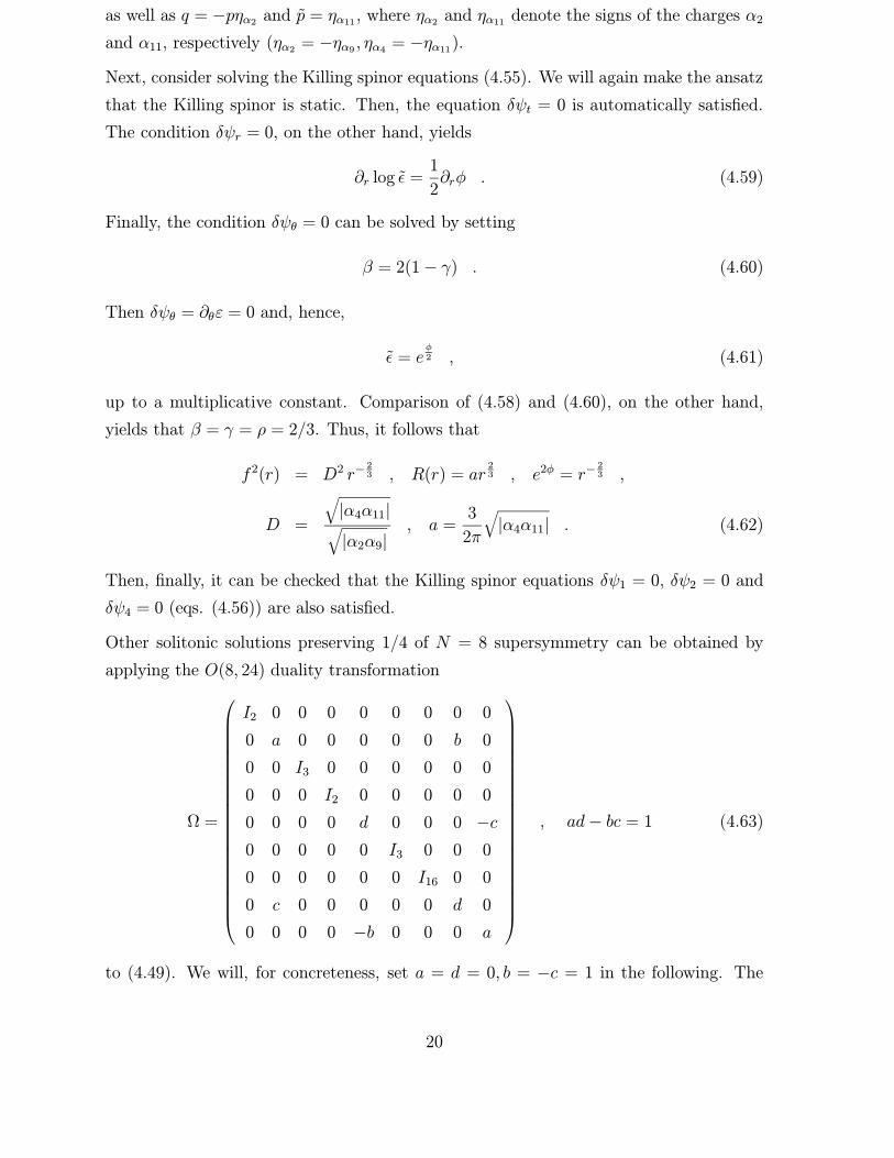
Other solitonic solutions preserving 1/4 of N = 8 supersymmetry can be obtained by

applying the O(8, 24) duality transformation

Ω =

I2 0 0 0 0 0 0 0 0

0 a 0 0 0 0 0 b 0

0 0 I3 0 0 0 0 0 0

0 0 0 I2 0 0 0 0 0

0 0 0 0 d 0 0 0 −c

0 0 0 0 0 I3 0 0 0

0 0 0 0 0 0 I16 0 0

0 c 0 0 0 0 0 d 0

0 0 0 0 −b 0 0 0 a

, ad− bc = 1 (4.63)

to (4.49). We will, for concreteness, set a = d = 0, b = −c = 1 in the following. The

20

resulting dual background fields G−1 and B are then given by

G11 G12 0 0 · · · 0G21 G22 0 0 · · · 00 0 G33 G34 · · ·

0 0 G43 G44 0...

.... . .

0 · · · 0 G77

=

G11 G12 0 0 · · ·G21 G22 0 0 · · · 00 0 e2φ −e2φΨ4 · · ·

0 0 −e2φΨ4 G44 + e2φΨ24 0

......

. . .0 · · · 0 G77

,

B =

0 B12 0 · · · 0B21 00 0 B34 0

0 B43 0...

... 0. . .

0 · · · 0

=

0 Υ9 0 · · · 0−Υ9 0

0 0 Ψ11 0

0 −Ψ11 0...

... 0. . .

0 · · · 0

,

as well as

e2φ = G33 , Ψ = 0 , aIm = 0 . (4.64)

Note that the dual dilaton field φ is constant.

It can be checked that the associated Killing spinor equations are satisfied by a constant

Killing spinor ε = ε⊗ χ provided that

Σ12χ = −i p ηα2χ , Σ34χ = −i p ηα4χ , (4.65)

where, again, ηα2 and ηα4 denote the sign of the charges α2 and α4, respectively.

4.4 Soliton solutions preserving N = 1 supersymmetry

It is now straightforward to construct solutions which preserve 1/8 of D = 3, N = 8

supersymmetry.

One class of solitonic solutions preserving 1/8 of D = 3, N = 8 supersymmetry is given

as follows. The background fields are given by

ema =

f2(r) −f2(r)Υ2 0 0 0 0 0

0√|α9

α2| 0 0 0 0 0

0 0 f4(r) −f4(r)Υ4 0 0 0

0 0 0√|α11

α4| 0 0 0

0 0 0 0√G55 0 0

0 0 0 0 0√G66 0

0 0 0 0 0 0√G77

, (4.66)

21

B =

0 B12 0 0 0 0 0B21 0 0 0 0 0 00 0 0 B34 0 0 00 0 B43 0 0 0 00 0 0 0 0 0 00 0 0 0 0 0 00 0 0 0 0 0 0

=

0 Υ9 0 0 0 0 0−Υ9 0 0 0 0 0 0

0 0 0 Υ11 0 0 00 0 −Υ11 0 0 0 00 0 0 0 0 0 00 0 0 0 0 0 00 0 0 0 0 0 0

as well as

e2φ = r−γ , Ψ =

Ψ1

...

Ψ6

Ψ7

Ψ8

...

Ψ13

Ψ14

Ψ15

...

=

0...

0

− θ2πα14

0...

0

− θ2πα7

0...

, aIm = 0 . (4.67)

Here

Υ2 = −θ

2πα9 , Υ4 = −

θ

2πα11 , Υ9 = −

θ

2πα2 , Υ11 = −

θ

2πα4 ,

G77 = |α7

α14

| (4.68)

as well as

f2 = D2 r− γ

2 , D2 =

√|α7α14|√|α2α9|

,

f4 = D4 r− γ

2 , D4 =

√|α7α14|√|α4α11|

. (4.69)

The space–time metric is given by

ds2 = −dt2 + dr2 +R2dθ2 , R = ar1− γ2 , (4.70)

where

a =1

γ π

√|α7α14| , γ =

1

2. (4.71)

The associated Killing spinor ε = ε⊗ χ satisfies (3.8) and (3.9) with

ε = eφ2 , (4.72)

22

as well as

Σ12χ = iqχ , Σ34χ = iqχ , Σ7χ = χ , q = ± , q = ± , (4.73)

where p = ηα14 , q = −pηα2 and q = −pηα4 (ηα2 = −ηα9 , ηα4 = −ηα11 , ηα7 = −ηα14).

Another class of solitonic solutions preserving 1/8 of D = 3, N = 8 supersymmetry is

given as follows. The background fields are given by

ema =

f2(r) −f2(r)Υ2 0 0 0 0 0

0√|α9

α2| 0 0 0 0 0

0 0 f4(r) −f4(r)Υ4 0 0 0

0 0 0√|α11

α4| 0 0 0

0 0 0 0 f6(r) −f6(r)Υ6 0

0 0 0 0 0√|α13

α6| 0

0 0 0 0 0 0√G77

,

B =

0 B12 0 0 0 0 0B21 0 0 0 0 0 00 0 0 B34 0 0 00 0 B43 0 0 0 00 0 0 0 0 B56 00 0 0 0 B65 0 00 0 0 0 0 0 0

=

0 Υ9 0 0 0 0 0−Υ9 0 0 0 0 0 0

0 0 0 Υ11 0 0 00 0 −Υ11 0 0 0 00 0 0 0 0 Υ13 00 0 0 0 −Υ13 0 00 0 0 0 0 0 0

(4.74)

as well as

e2φ = r−γ , Ψ =

Ψ1

...

Ψ6

Ψ7

Ψ8

...

Ψ13

Ψ14

Ψ15

...

=

0...

0

− θ2πα14

0...

0

− θ2πα7

0...

, aIm = 0 . (4.75)

Here

Υ2 = −θ

2πα9 , Υ4 = −

θ

2πα11 , Υ6 = −

θ

2πα13 ,

Υ9 = −θ

2πα2 , Υ11 = −

θ

2πα4 , Υ13 = −

θ

2πα6 ,

G77 = |α7

α14| (4.76)

23

as well as

f2 = D2 r− γ

2 , D2 =

√|α7α14|√|α2α9|

,

f4 = D4 r− γ

2 , D4 =

√|α7α14|√|α4α11|

,

f6 = D6 r− γ

2 , D6 =

√|α7α14|√|α6α13|

. (4.77)

The space–time metric is given by

ds2 = −dt2 + dr2 +R2dθ2 , R = ar1− γ2 , (4.78)

where

a =1

γ π

√|α7α14| , γ =

2

5. (4.79)

The associated Killing spinor ε = ε⊗ χ satisfies (3.8) and (3.9) with

ε = eφ2 , (4.80)

as well as

Σ12χ = iqχ , Σ34χ = iqχ , Σ56χ = iqχ , Σ7χ = χ , q = ± , q = ± , q = ±, (4.81)

where p = ηα14 , q = −pηα2 , q = −pηα4 and q = −pηα6 (ηα2 = −ηα9 , ηα4 = −ηα11 , ηα6 =

−ηα13 , ηα7 = −ηα14).

5 Supersymmetric solutions with ~α2 = 0

In this section, we will consider a particular class of solutions to the Killing spinor

equations, namely solutions for which ~α2 = αTLα = 0. We will construct solutions

which preserve 1/2m of N = 8, D = 3 supersymmetry, where m = 1, 2, 3. The solutions

are obtained with Hµνρ = 0 and aIm = 0.

We will find that the space–time metric (3.3) is given in terms of

V = 1, R = a r1−γ , (5.1)

and that the dilaton is given by

e2φ = r−γ , (5.2)

24

where

γ =2

n+ 2, a =

|αi|

2π γ. (5.3)

By the coordinate transformation r = (γ)1γ (a ln r)

1γ , 1 ≤ r ≤ ∞, the associated space–

time metric can be put into the form

ds2 = −dt2 + a2γ (γ)

2(1−γ)γ

(ln r)

r2

2(1−γ)γ

(dr2 + r2dθ2). (5.4)

The curvature scalar, R = gµνRµν , is computed to be

R = 2γ(1− γ)1

r2=

4n

(n+ 2)2

1

r2. (5.5)

5.1 Electrically charged solutions

We will be solving the same Killing spinor equations subject to the same assumptions as

in subsection 4.1, where in addition we take α9 = 0.

Looking back at (4.9), with α9 = 0, i.e. F(2)µν2 = 0, we have ∂rφ = −∂r ln

√G22. From

(4.16) we still have ∂rφ = −∂r lnR.

These relations can be satisfied with the following ansatz√G22 = de−φ, R = a e−φ, (5.6)

where d is an integration constant that is set to one in the following.

We can now solve equations (4.10), (4.11) and find, (with again V = 1),√G22 = r

13 ,

R =a

cr

13 ,

a

c3= −

3 p α2

4π,

e2φ = c2r−23 , (5.7)

where pα2 = −|α2| and where the integration constant c will be set to one.

The space–time metric is now of the form

ds2 = −dt2 + dr2 + a2 r23 dθ2. (5.8)

or, equivalently,

ds2 = −dt2 +2a3

3

(ln r

r2

)(dr2 + r2dθ2) , (5.9)

25

where r = (2a3

)3/2

(ln r)3/2.

The dependence of the spinor in terms of φ is the same as before

∂r ε−1

2∂rφ ε = 0 ,

∂θ ε = 0 , (5.10)

or

ε = eφ2 = r−

16 . (5.11)

These electric solutions preserve again 1/2 of the N = 8 supersymmetry.

5.2 Soliton solutions preserving N = 4 supersymmetry

Now we discuss the soliton solution which is obtained by dualizing the charged

solution discussed in subsection 5.1, with one electric charge only (α9 =

0). The bosonic background fields of the charged solution are given by

φ, (Gmn) = diagonal (G11, G22, . . . , G77) , G22 = r23 , Bmn = 0, aIm = 0 and ΨT =

(0, 0, 0, . . . , 0,Ψ9, 0, . . . , 0) = (0, 0 , 0, . . . , 0, − θ2πα2 , 0, . . . , 0). We will utilize the

O(8, 24) transformation Ω given in (2.19) to generate the dual backgroundM→ ΩMΩT .

We will for simplicity set the transformation parameter d to d = 0 in the following so

that bc = −1. The dual background fields are then given by

G−1 =

G11 0 0 · · · 0

0 G22 0 · · · 0

0 0 G33 0 · · ·...

.... . .

0 · · · 0 G77

=

b2e2φ 0 0 · · · 0

0 G22 0 · · · 0

0 0 G33 0 · · ·...

.... . .

0 · · · 0 G77

,

B = (Bmn) =

0 B12 0 · · · 0

B21 0

0 0...

.... . .

0 · · · 0

=

0 −cΨ9 0 · · · 0

cΨ9 0

0 0...

.... . .

0 · · · 0

(5.12)

as well as

e2φ = c2G11 , Ψ =

Ψ1

Ψ2

...

Ψ9

...

=

−a/c

0...

0...

, aIm = 0 . (5.13)

26

The associated gauge field strengths F (a)µν are again all zero for this solitonic solution.

The internal inverse vielbein ema associated to (5.12) is given by

ema =

beφ 0 0 · · · 0

0√G22 0 · · · 0

0 0√G33 0 · · ·

......

. . .

0 · · · 0√G77

. (5.14)

Note that the space–time metric is duality invariant and hence given as in (5.8).

The Killing spinor equations in the new background (5.12) are of the same form as in

equations (4.29), (4.30) and (4.31). It is easy to check that the Killing spinor will be of

the same form as before with the same conditions (3.8), (3.9) and (4.33) to be satisfied.

For the solitonic background under consideration, the Killing spinor equation (4.29) then

yields

−p ∂r log det eam + b q

√G22

Reφ∂θB12 = 0 , (5.15)

which is satisfied, provided one takes q = pp.

Next, consider solving the Killing spinor equations (4.30). The Killing spinor being static,

the equation δψt = 0 is again automatically satisfied. The condition δψr = 0 yields again

∂rε = 0 . (5.16)

Finally, the condition δψθ = 0 results in

∂θε−1

2∂rRγ

12ε−1

4

√G22eφ∂θΨ9Σ12ε = 0 , (5.17)

from which it follows again, if pp = q, that

∂θε = 0 . (5.18)

Hence the Killing spinor ε is constant.

Finally, it can be checked that the Killing spinor equations (4.31) for δψ1 and δψ2 are

automatically satisfied.

The solitonic background preserves 1/2 of N = 8 supersymmetry.

27

5.3 Soliton solutions preserving N = 2 supersymmetry

We take the following ansatz for the background fields G−1 and B

G11 0 0 0 · · · 00 G22 0 0 · · · 00 0 G33 0 · · ·

0 0 0 G44 0...

.... . .

0 · · · 0 G77

=

f 21 (r) 0 0 0 · · · 00 f 2

2 (r) 0 0 · · · 00 0 G33 0 · · ·

0 0 0 f 24 (r) 0

......

. . .0 · · · 0 G77

,

B = (Bmn) =

0 B12 0 · · · 0B21 0

0 0...

.... . .

0 · · · 0

=

0 Υ9 0 · · · 0−Υ9 0

0 0...

.... . .

0 · · · 0

, (5.19)

where

f 2i (r) =

D2i

rγ, D4 = 1, Υ9 = −

θ

2πα2 . (5.20)

We will also take

e2φ = r−γ , Ψ =

Ψ1

Ψ2

Ψ3

Ψ4

Ψ5

...

Ψ10

Ψ11

Ψ12

...

=

0

0

0

0

0...

0

− θ2πα4

0...

, aIm = 0 . (5.21)

For the space–time metric we will make the ansatz

ds2 = −dt2 + dr2 +R2(r) dθ2 , R(r) = a r1−γ . (5.22)

The constants Di and γ will be fixed by the Killing spinor equations.

The Killing spinor equations (3.2) now take the form

δχI = 0 ,

δλ = −1

2e−φ∂µφ+ ln det eamγ

µ ε+1

4e−φ∂µBmnγ

µ ⊗ Σmnε , (5.23)

28

δψµ = ∂µε+1

4ωµαβγ

αβε+1

4(eµαe

νβ−eµβe

να)∂νφγ

αβε

+1

4e−φ emaF

(1)mµν γνγ4 ⊗ Σaε−

1

8∂µBmnΣmnε , (5.24)

δψd = −1

4e−φ(emd ∂µema+ema ∂µemd)γ

µγ4 ⊗ Σaε+1

4e−φemd e

na∂µBmnγ

µγ4 ⊗ Σaε

−1

8e−2φ emdF

(1)mµν γµνε . (5.25)

The Killing spinor ε = ε⊗χ will be taken to satisfy (3.8) and (3.9) as well as Σ12 χ = iq χ

and Σ4 χ = χ.

The condition δλ = 0 (5.23) then implies

D1D2 = −pqγ2πa

α2, (5.26)

while δψθ = 0 in (5.24) gives the condition

pa(1−3

2γ) +

qα2

4πD1D2 = 0 . (5.27)

These last two equations yield γ = 12, whereas δψ4 = 0 (5.25) gives the relation

a = −α4

2πγp. (5.28)

Since this last quantity is positive, this implies p = −ηα4 , where ηα4 denotes the sign of

α4.

The above shows that we can then take

D1 = D2 =

√−pqγ2πa

α2

=

√γ2πa

|α2|, (5.29)

with −pq = ηα2 .

This solution preserves 1/4 of N = 8 supersymmetry.

5.4 Soliton solutions preserving N = 1 supersymmetry

It is now straightforward to construct solutions which preserve 1/8 of D = 3, N = 8

supersymmetry.

One class of solitonic solutions preserving 1/8 of D = 3, N = 8 supersymmetry is given

as follows. The background fields G−1 and B are given by

G11 0 0 0 0 0 00 G22 0 0 0 0 00 0 G33 0 0 0 00 0 0 G44 0 0 00 0 0 0 G55 0 00 0 0 0 0 G66 00 0 0 0 0 0 G77

=

f 21 (r) 0 0 0 0 0 00 f 2

2 (r) 0 0 0 0 00 0 G33 0 0 0 00 0 0 f 2

4 (r) 0 0 00 0 0 0 f 2

5 (r) 0 00 0 0 0 0 f 2

6 (r) 00 0 0 0 0 0 G77

,

29

0 B12 0 0 0 0 0B21 0 0 0 0 0 00 0 0 0 0 0 00 0 0 0 0 0 00 0 0 0 0 B56 00 0 0 0 B65 0 00 0 0 0 0 0 0

=

0 Υ9 0 0 0 0 0−Υ9 0 0 0 0 0 0

0 0 0 0 0 0 00 0 0 0 0 0 00 0 0 0 0 Υ13 00 0 0 0 −Υ13 0 00 0 0 0 0 0 0

,

where

f 2i (r) =

D2i

rγ, D4 = 1, Υ9 = −

θ

2πα2 , Υ13 = −

θ

2πα6 . (5.30)

Again, we have

e2φ = r−γ , Ψ =

Ψ1

Ψ2

Ψ3

Ψ4

Ψ5

...

Ψ10

Ψ11

Ψ12

...

=

0

0

0

0

0...

0

− θ2πα4

0...

, aIm = 0 . (5.31)

As before, we will make the following ansatz for the space–time metric

ds2 = −dt2 + dr2 +R2(r) dθ2 , R(r) = a r1−γ . (5.32)

Now, the Killing spinor equations give the following constraints

−2γp−α2q

2πaD1D2 −

α6q

2πaD5D6 = 0,

pa(1−3

2γ) +

qα2

4πD1D2 +

qα6

4πD5D6 = 0, (5.33)

as well as

D1D2 = −pq2πaγ

α2

, D5D6 = −pq2πaγ

α6

and a = −α4p

2πγ. (5.34)

Here we have used the conditions

Σ4χ = χ ,

Σ12χ = iqχ, q = −pηα2 ,

Σ56χ = iqχ, q = −p ηα6 , (5.35)

30

which shows that the background preserves 1/8 of the N = 8 supersymmetry.

Note that equation (5.33) yields that γ here is 25.

Looking back at Bmn we notice now that we can add one more block with B37 = −B73 =

Υ14 = − θ2πα7. The Killing equations will imply a further condition on χ,

Σ37χ = iq χ, q = −p ηα7 . (5.36)

Furthermore γ = 1/3 and D3D7 = −pq 2πaγα7

. We note that the condition (5.36) does not

break any additional supersymmetry, and hence this solution also preserves 1/8 of the

N = 8 supersymmetry.

6 The compactified cosmic string solution

In [3], Sen constructed a particular three-dimensional solution by considering the funda-

mental string solution of the four-dimensional theory [22] and by winding the direction

along which the string extends once in the third direction. As shown in [3], this solution is

related to the cosmic string solution of [34] by a O(8,24;Z) transformation. Other three-

dimensional solutions with internal winding can be obtained from the four-dimensional

string solutions given in [35].

The fundamental string solution in four space–time dimensions is known to have partial

space–time supersymmetry [36]. Here, we will presently construct the Killing spinor

associated with the particular three-dimensional solution mentioned above.

The field configuration representing a fundamental string solution winding once in the

third direction is described below, following [3].

The three-dimensional space–time metric is now of the form

ds2 = −dt2 + λ2 (dr2 + r2 dθ2)

= −dt2 + λ2 dzdz , (6.1)

where z = reiθ is the complex coordinate labelling the two-dimensional space. The scalar

fields are e−2φ = λ2, Ψ ≡ Ψ1 = −λ1 and G11 = e2φ. From (2.11), the only non-vanishing

field strength is

F(2)µν1 = e4φεαβγ eµα eνβ e

ργ∂ρΨ . (6.2)

It will turn out to be convenient to combine λ1 and λ2 into a complex scalar field S =

λ1 + iλ2. Here, as opposed to the previous cases, we take Ψ and φ to depend on both r

and θ.

31

With these assignments the Killing spinor equations take the form (where now Σ1χ = χ),

δλ = −(∂rφ γ1 +

1

r∂θφ γ

2) ε+1

2e2φ(∂rΨ γ1 +

1

r∂θΨγ

2) J γ4 ε ,

δψt = −1

2eφ(−∂rφ γ

2 +1

r∂θφ γ

1) J ε+1

4e3φ(−∂rΨ γ2 +

1

r∂θΨ γ1)γ4ε ,

δψr = ∂r ε−1

4

e2φ

r∂θΨ γ0γ4ε ,

δψθ = ∂θ ε−1

2γ12 ε+

r

4e2φ∂rΨ γ0γ4ε ,

δψ1 = −1

2(∂rφ γ

1 +1

r∂θφ γ

2) γ4 ε−1

4e2φ(∂rΨ γ1 +

1

r∂θΨ γ2) J ε . (6.3)

Compatibility of the form of ε for δλ, δψt and δψ1 can be achieved by imposing Jγ4 ε =

iα ε, which yields ε1

ε2

ε3

ε4

=

ε1

ε2

−iαε1

−iαε2

, (6.4)

where α = ±.

Equations δλ, δψt and δψ1 are actually equivalent to each other and can be written in

the form

δλ ∝ ∂µS γµ ε (6.5)

with S = −Ψ + ie−2φ, provided that α = +1.

The equation δλ = 0 can be solved by assuming that S is a holomorphic function of

z, therefore ∂zS = 0. Note that a holomorphic function S(z) solves the equation of

motion (2.8).

Then, δλ ∝ ∂zS γz ε = 0, which can be solved by setting γz ε = 0.

By using that γz ∝ γ1(1 + i)− γ2(1− i), one findsε1

ε2

ε3

ε4

= ε

1

i

−i

1

. (6.6)

The remaining equations to be solved are then δψr = 0 and δψθ = 0. We find

∂r ε+1

4

e2φ

r∂θΨ ε = 0 ,

∂θ ε−i

2ε−

r

4e2φ∂rΨ ε = 0. (6.7)

32

The holomorphicity of S implies the relations

∂rΨ =2

re−2φ ∂θφ ,

1

r∂θΨ = −2∂rφ e

−2φ , (6.8)

which we use to solve for the spinors completely:

ε = eφ2 e

i2θ. (6.9)

The above solution breaks 1/2 of N = 8, D = 3 supersymmetry.

7 String solutions with Hµνρ 6= 0

Here we show how the Killing spinor equations (3.2) determine a three-dimensional solu-

tion with a non-vanishing Hµνρ and a non-constant dilaton (other solutions with non-zero

Hµνρ have been considered in [37, 38]).

We consider a solution without gauge fields and with constant internal metric Gmn. We

will take Hµνρ =√−gεµνρΛepφ, where p is an integer, in the Einstein frame. We will take

the space–time metric to be of the form (3.3), and we will also take φ = φ(r).

The Killing spinor equations reduce to

δχI = 0 ,

δλ = −1

2e−φ∂µ(φ+ ln det eam)γµ ε+

1

12e−3φHµνρ γ

µνρ ε ,

δψµ = ∂µε+1

4ωµαβγ

αβε+1

4(eµαe

νβ − eµβe

να)∂νφγ

αβε−1

8e−2φHµνδγ

νδε ,

δψd = −1

4e−φ(emd ∂µema+ema ∂µemd)γ

µγ4 ⊗ Σaε . (7.1)

By using identity (A.11) of the appendix, these equations become

δχI = 0 ,

δλ = −1

2e−φ∂r(φ+ ln det eam)

√V γ1 ε+

1

2e(p−3)φΛ J ε ,

δψt =1

2[√V ∂r√V + V ∂rφ] J γ2 ε+

1

4e(p−2)φ

√V Λ Jγ0 ε ,

δψr = ∂rε−1

4e(p−2)φ Λ

√VJγ1 ε ,

δψθ = ∂θε−1

2[√V ∂rR+R

√V ∂rφ] J γ0 ε−

1

4e(p−2)φRΛ Jγ2ε . (7.2)

33

Compatibility of the spinor ε = ε⊗ χ within these equations is obtained by demanding

γ1 ε = α J ε , α = ± ,

γ2 ε = −α γ0 ε . (7.3)

Then, one has

δλ = −1

2αe−φ∂r(φ+ ln det eam)

√V J ε+

1

2e(p−3)φΛ J ε ,

δψt = −1

2α[√V ∂r√V + V ∂rφ] J γ0 ε+

1

4e(p−2)φ

√V Λ Jγ0 ε ,

δψr = ∂rε−1

4αe(p−2)φ Λ

√Vε ,

δψθ = ∂θε−1

2[√V ∂rR+R

√V ∂rφ] J γ0 ε+

α

4e(p−2)φRΛ Jγ0ε . (7.4)

For α = +1 the spinor ε is of the formε1

ε2

ε3

ε4

=

ε1

0

ε3

0

= ε

1

0

1

0

, (7.5)

(where we have imposed ε1 = ε3 in order to reduce the degrees of freedom contained in ε

to the degrees of freedom contained in a two component spinor, see appendix), whereas

for α = −1 it is ε1

ε2

ε3

ε4

=

0

ε2

0

ε4

= ε

0

1

0

1

. (7.6)

Demanding the vanishing of the Killing spinor equations (7.4) and imposing the condition

∂θ ε = 0, as well as αΛ = |Λ|, leaves us with the following constraints

√V ∂rφ = e(p−2)φ|Λ| ,

√V ∂r√V + V ∂rφ =

1

2

√V e(p−2)φ|Λ| ,

∂r ε =1

4

|Λ|√Ve(p−2)φε ,

√V ∂rR+R

√V ∂rφ =

1

2e(p−2)φ|Λ| . (7.7)

34

These equations can be solved to give

V = a2 e−φ ,

R = b2 e−φ/2 ,

ε = eφ4 ε0, (7.8)

where a, b, ε0 are integration constants.

For p 6= 32, the dilaton is given by

e( 32−p)φ = |

Λ

a(3

2− p)(r − r0)|, (7.9)

whereas for p = 32,

∂rφ =|Λ|

a−→ φ =

|Λ|

a(r − r0). (7.10)

Note that ε is real and hence the background preserves 1/2 of N = 8, D = 3 supersym-

metry.

We notice here that whatever the value of p, there is a solution to the Killing spinor

equations. On the other hand, the equations of motion are satisfied provided Hµνρ =εµνρ√−g Λ e4φ, that is p = 4. Thus, contrary to common experience [23, 13, 14], not every

solution to the Killing spinor equations solves the equations of motion.

For p = 4, the curvature scalar is computed to be R = 52Λ2e4φ, which is always positive.

8 Conclusions

We have considered in the present work the low-energy effective Lagrangian of heterotic

string theory compactified on a seven-torus, and we have constructed a variety of electri-

cally charged and solitonic backgrounds preserving 1/2m of N = 8, D = 3 supersymmetry

(m = 1, 2, 3). The construction of the solutions is done by using the criteria of unbroken

supersymmetries and solving for the associated Killing spinor equations. The space–time

line elements of the solutions constructed here have the form (4.4), which differ from the

usual line element associated with conical geometries [12]. These line elements do not

seem to correspond to small deformations of flat space–time. Thus they seem to contain

some interesting structure which deserves further study.

Further solitonic solutions with diagonal space–time line elements can be obtained by

applying more general O(8, 24) transformations to the electrically charged solutions of

section 4 and 5. It would also be interesting to consider a non-diagonal ansatz for the

space–time metric.

35

We have also found a solution to the Killing spinor equations with Hµνρ 6= 0 which

preserves 1/2 of the N = 8 supersymmetry. Furthermore, we have shown that the

compactified cosmic string solution constructed by Sen [3] satisfies our Killing spinor

equations.

Most of the solutions presented here are charged with the associated gauge field strengths

given everywhere by (2.13). We note, however, that one should generally expect these

solitonic solutions to get modified by quantum corrections, at least in the strong coupling

regime [3]. Recall the fundamental string solution discussed by Sen [3] that we have

considered in section 6. There we showed that a holomorphic solution S(z) satisfies our

Killing spinor equations. As Sen points out, the holomorphic function S(z) = λ1 + iλ2

has the behavior λ2 = e−2φ ∼ − ln r for r −→ 0, whereas at r −→ ∞, this behavior

needs to be modified in order to make sense. This is achieved by replacing S by the

SL(2,Z) invariant function j(S), such that j(S(z)) ' 1/z for r −→ ∞. Therefore the

solution S(z) should be considered only as an approximate solution that gets modified

as the theory enters the strong coupling regime. In analogy with the above, we would,

for example, expect our electrically charged solutions in subsections 4.1 and 5.1 to get

modified at short distances, where the coupling becomes strong. Similar phenomena

have been shown to occur in N = 4, D = 3 supersymmetric gauge theories [39], where

the classical moduli space receives perturbative as well as non-perturbative quantum

corrections. An extension of these ideas to string theory remains to be explored.

Acknowledgement

We would like to thank Tomas Ortin for helpful discussions.

A Appendix

In ten dimensions, the ΓA matrices satisfy

ΓA,ΓB = 2ηAB , (A.1)

where A,B are D=10 tangent space indices and where ηAB = (−,+, . . . ,+). The decom-

position of the gamma matrices that is appropriate to the 10=3+7 split is

ΓA ≡ (Γα,Γa) = (γα ⊗ I8, γ4 ⊗ Σa) , (A.2)

where

γα, γβ = 2ηαβ, ηαβ = (−,+,+) ,

36

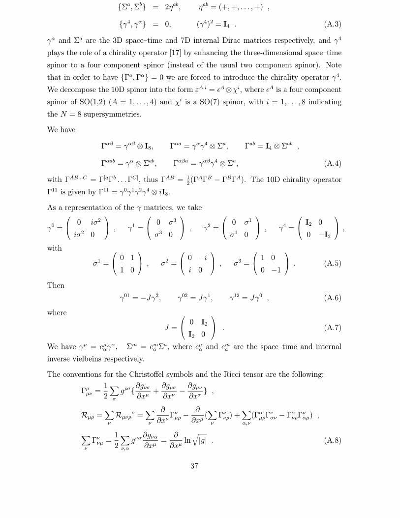
Σa,Σb = 2ηab, ηab = (+,+, . . . ,+) ,

γ4, γα = 0, (γ4)2 = I4 . (A.3)

γα and Σa are the 3D space–time and 7D internal Dirac matrices respectively, and γ4

plays the role of a chirality operator [17] by enhancing the three-dimensional space–time

spinor to a four component spinor (instead of the usual two component spinor). Note

that in order to have Γa,Γα = 0 we are forced to introduce the chirality operator γ4.

We decompose the 10D spinor into the form εA,i = εA⊗χi, where εA is a four component

spinor of SO(1,2) (A = 1, . . . , 4) and χi is a SO(7) spinor, with i = 1, . . . , 8 indicating

the N = 8 supersymmetries.

We have

Γαβ = γαβ ⊗ I8, Γαa = γαγ4 ⊗ Σa, Γab = I4 ⊗ Σab ,

Γαab = γα ⊗ Σab, Γαβa = γαβγ4 ⊗ Σa, (A.4)

with ΓAB...C = Γ[aΓb . . .ΓC], thus ΓAB = 12(ΓAΓB − ΓBΓA). The 10D chirality operator

Γ11 is given by Γ11 = γ0γ1γ2γ4 ⊗ iI8.

As a representation of the γ matrices, we take

γ0 =

0 iσ2

iσ2 0

, γ1 =

0 σ3

σ3 0

, γ2 =

0 σ1

σ1 0

, γ4 =

I2 0

0 −I2

,

with

σ1 =

0 1

1 0

, σ2 =

0 −i

i 0

, σ3 =

1 0

0 −1

. (A.5)

Then

γ01 = −Jγ2, γ02 = Jγ1, γ12 = Jγ0 , (A.6)

where

J =

0 I2

I2 0

. (A.7)

We have γµ = eµαγα, Σm = ema Σa, where eµα and ema are the space–time and internal

inverse vielbeins respectively.

The conventions for the Christoffel symbols and the Ricci tensor are the following:

Γρµν =1

2

∑σ

gρσ∂gνσ∂xµ

+∂gµσ∂xν

−∂gµν∂xσ ,

Rµρ =∑ν

Rµνρν =

∑ν

∂

∂xνΓνµρ −

∂

∂xµ(∑ν

Γννρ) +∑α,ν

(ΓαµρΓναν − ΓανρΓ

ναµ) ,

∑ν

Γννµ =1

2

∑ν,α

gνα∂gνα

∂xµ=

∂

∂xµln√|g| . (A.8)

37

Our convention for the spin connection is

ωMAB =1

2ENA (∂MENB−∂NEMB)+

1

2ENB (∂NEMA−∂MENA)−

1

2EPAE

QB (∂PE

CQ−∂QE

CP )EMC

(A.9)

and

GMN = EAM ηAB E

BN , EMB = EC

M ηCB. (A.10)

Other useful identities are

εµνρ γµνρ =

1

det eεαβη γ

αβη

=6

det eε012 γ

012 with ε012 = −ε012 = 1 ,

εµνρ γνρ =

1

det eeαµ εαβη γ

βη . (A.11)

References

[1] S. Carlip, gr-qc/9503024.

[2] S. Carlip, Class. Quant. Grav. 12 (1995) 2853, gr-qc/9506079.

[3] A. Sen, Nucl. Phys. B434 (1995) 179, hep-th/9408083.

[4] I. Bakas, Phys. Lett. B343 (1995) 103, hep-th/9410104.

[5] A. Herrera-Aguilar and O. Kechkin, hep-th/9704083.

[6] E. Witten, Int. J. Mod. Phys. A10 (1995) 1247, hep-th/9409111.

[7] E. Witten, Mod. Phys. Lett. A10 (1995) 2153, hep-th/9506101.

[8] K. Becker, M. Becker and A. Strominger, Phys. Rev. D51 (1995) 6603, hep-

th/9502107.

[9] S. Forste and A. Kehagias, hep-th/9610060.

[10] J. M. Izquierdo and P. K. Townsend, Class. Quant. Grav. 12 (1995) 895, gr-

qc/9501018.

[11] P. S. Howe, J. M. Izquierdo, G. Papadopoulos and P. K. Townsend, Nucl. Phys.

B467 (1996) 183, hep-th/9505032.

38

[12] S. Deser, R. Jackiw and G. ’t Hooft, Annals Phys. 152 (1984) 220.

[13] J. D. Edelstein, C. Nunez and F. A. Schaposnik, Nucl. Phys. B458 (1996) 165,

hep-th/9506147.

[14] J. D. Edelstein, C. Nunez and F. A. Schaposnik, Phys. Lett. B375 (1996) 163,

hep-th/9512117.

[15] J. D. Edelstein, Phys. Lett. B390 (1997) 101, hep-th/9610163.

[16] G.W. Gibbons, M.B. Green and M.J. Perry, Phys. Lett. B370 (1996) 37, hep-

th/9511080.

[17] C. Wetterich, Nucl. Phys. B222 (1983) 20.

[18] M. Cvetic and D. Youm, Phys. Rev. D53 (1996) 584, hep-th/9507090; Nucl. Phys.

B438 (1995) 182, Nucl. Phys. B449 (1995) 146, hep-th/9409119.

[19] G. Horowitz, in ‘String theory and quantum gravity’ (Trieste 1992), p. 55, hep-

th/9210119.

[20] M. Banados, C. Teitelboim and Z. Zanelli, Phys. Rev. Lett. 69 (1992) 1849, hep-

th/9204099.

[21] G. W. Gibbons, in ‘Supersymmetry, Supergravity and Related Topics’, eds. F. del

Aguila, J. de Azcarraga and L. Ibanez (World Scientific, Singapore 1985), p. 147.

[22] A. Dabholkar, G. Gibbons, J. Harvey and F. R. Ruiz, Nucl. Phys. B340 (1990) 33;

A. Dabholkar and J. A. Harvey, Phys. Rev. Lett. 63 (1989) 719.

[23] W. Boucher, Phys. Lett. 132B (1983) 88.

[24] S. Ferrara, C. Kounnas and M. Porrati, Phys. Lett. B181 (1986) 263;

M. Terentev, Sov. J. Nucl. Phys. 49 (1989) 713.

[25] J. Maharana and J. H. Schwarz, Nucl. Phys. B390 (1993) 3, hep-th/9207016;

S. Hassan and A. Sen, Nucl. Phys. B375 (1992) 103, hep-th/9109038.

[26] N. Marcus and J. Schwarz, Nucl. Phys. B228 (1983) 145.

[27] A. Sen, Int. J. Modern Physics A9 (1994) 3707, hep-th/9402002.

[28] E. Cremmer and B. Julia, Nucl. Phys. B159 (1979) 141.

[29] A. Strominger, Nucl. Phys. B343 (1990) 167; Nucl. Phys. B274 (1986) 253.

39

[30] P. Candelas, G. Horowitz, A. Strominger and E. Witten, Nucl. Phys. B258 (1985)

46.

[31] J. A. Harvey and J. Liu, Phys. Lett. B268 (1991) 40.

[32] A. Peet, Nucl. Phys. B456 (1995) 732, hep-th/9506200.

[33] M. Henneaux, Phys. Rev. D29 (1984) 2766.

[34] B. Greene, A. Shapere, C. Vafa and S.–T. Yau, Nucl. Phys. B337 (1990) 1.

[35] M. J. Duff, S. Ferrara, R. R. Khuri and J. Rahmfeld, Phys. Lett. B356 (1995) 479,

hep-th/9506057.

[36] A. Sen, Nucl. Phys. B388 (1992) 457, hep-th/9206016.

[37] J. H. Horne and G. Horowitz, Nucl. Phys. B368 (1992) 444, hep-th/9108001.

[38] G. Horowitz and D. L. Welch, Phys. Rev. Lett. 71 (1993) 328, hep-th/9302126.

[39] N. Seiberg and E. Witten, hep-th/9607163.

40