arX

iv:h

ep-t

h/00

1121

7v2

4 F

eb 2

001

DTP/00/101, UPR-908-T, ITFA-2000-31

HIP-2000-63/TH, hep-th/0011217

Supersymmetric Conical Defects:Towards a string theoretic description of black hole formation

Vijay Balasubramanian1∗, Jan de Boer2†, Esko Keski-Vakkuri3‡ and Simon F. Ross4§

1David Rittenhouse Laboratories, University of Pennsylvania,

Philadelphia, PA 19104, USA

2Instituut voor Theoretische Fysica,

Valckenierstraat 65, 1018XE Amsterdam, The Netherlands

3Fysiikan tutkimuslaitos, Helsingin Yliopisto,

PL 9, FIN-00014 Helsingin Yliopisto, Finland

4 Centre for Particle Theory, Department of Mathematical Sciences

University of Durham, South Road, Durham DH1 3LE, U.K.

Abstract

Conical defects, or point particles, in AdS3 are one of the simplest non-

trivial gravitating systems, and are particularly interesting because black holes

can form from their collision. We embed the BPS conical defects of three

dimensions into the N = 4b supergravity in six dimensions, which arises from

IIB string theory compactified on K3. The required Kaluza-Klein reduction

of the six dimensional theory on a sphere is analyzed in detail, including the

relation to the Chern-Simons supergravities in three dimensions. We show that

the six dimensional spaces obtained by embedding the 3d conical defects arise

in the near-horizon limit of rotating black strings. Various properties of these

solutions are analyzed and we propose a representation of our defects in the

CFT dual to asymptotically AdS3 × S3 spaces. Our work is intended as a first

step towards analyzing colliding defects that form black holes.

∗vijay@endive.hep.upenn.edu†jdeboer@wins.uva.nl‡keskivak@rock.helsinki.fi§S.F.Ross@durham.ac.uk

1

1 Introduction

Twenty-five years after Hawking showed that black holes emit thermal radiation [1],

the apparent loss of quantum mechanical unitarity in the presence of a black hole

remains an outstanding problem for theoretical physics. We expect that this “infor-

mation puzzle”, which represents a fundamental tension between general relativity

and quantum mechanics, should either be erased or explained in a quantum theory of

gravity. In recent years string theory has explained microscopically the huge degen-

eracy required to account for the entropy of certain extremal black holes. However,

there has been no insight into why this degeneracy of states is related to something

geometric like the area of a horizon. More fundamentally, the information puzzle

remains exactly that – a puzzle.

This paper is the first in a series investigating the black hole information puzzle

in the context of string theory. In General Relativity, the simplest context for black

hole formation is gravity in three dimensions where there are no local dynamics.

In the presence of a negative cosmological constant, 3d gravity possesses black hole

solutions [2]. There is also a family of conical defects, the so-called point particles [3].

These solutions interpolate between the vacuum solution (AdS3 with mass M = −1

in conventional units) and the black hole spectrum which starts at M = 0. Exact

solutions of 3d gravity are known in which the collision of conical defects forms a black

hole [4]. We would like to use these simple classical processes to study the formation of

higher dimensional black holes in string theory. To this end, we must first embed the

conical defects supersymmetrically in a higher dimensional gravity arising from string

theory. Preserving supersymmetry is important because the controlled quantization

of black holes and solitons in string theory usually requires supersymmetry. The

presence of the negative cosmological constant in three dimensions suggests that there

should be a dual description of such spaces in terms of a two-dimensional conformal

field theory [5]. Our goal is to find such a dual picture and describe in it the process

of black hole formation from collision of conical defects. In [6] it was shown that the

3d conical defects and their collisions can be detected in correlation functions of the

dual CFT. Here we are interested in the direct description of the defects as objects

in the dual.1

Type IIB supergravity compactified on K3 yields the chiral N = 4b supergravity

in six dimensions, coupled to 21 tensor multiplets. This theory has classical solutions

with the geometry of AdS3×S3. In Sec. 2 we will construct supersymmetric solutions

where the sphere is fibered over AdS3 so that a minimum length circuit around the

AdS3 base leads to a rotation of the sphere around an axis. Since AdS3 is simply

connected, the fibre must break down at a point. Upon dimensional reduction to

the base this produces supersymmetric conical defects in three dimensions. In fact,

1It would also be interesting to make contact with the investigations of spherical shells in [7].

2

the identical objects have been obtained previously as solutions to extended 2 + 1

supergravity in the Chern-Simons formulation [8, 9]. The U(1) Wilson lines used in

these constructions to obtain a BPS solution arise in our case from the Kaluza-Klein

gauge field associated with the fibration. Our Kaluza-Klein ansatz for reducing the

action and equations of motion of 6d gravity to the 3d base does not yield precisely

a Chern-Simons theory. Nevertheless, the dimensionally reduced system admits solu-

tions with vanishing field strength, for which the analysis of supersymmetry remains

unchanged – the holonomy of Killing spinors under the spin connection is cancelled by

the holonomy under the gauge connection. Various details of sphere compactifications

of 6d, N = 4b supergravity are reviewed in the main text and the appendices.2

It is well-known that a horospheric patch of the AdS3 × S3 geometry can be

obtained as a near-horizon limit of the black string soliton of 6d supergravity [12].

Compactifying the extremal string solution on a circle yields the black holes of five

dimensional string theory whose states were counted in the classic paper [13].3 The

near-horizon limit of these solutions yields the BTZ black holes times S3 [12]. In

Sec. 3 we show that the fibered S3 solutions described above arise as the near-horizon

geometries of an extremal limit of spinning 6-dimensional strings compactified on a

circle. Interestingly, when the angular momentum is suitably chosen, global AdS3×S3

is recovered as a solution. We discuss various properties of the solution, including the

nature of the conical singularity and potential Gregory-Laflamme instabilities in the

approach to extremality.

The near-horizon limit of the six dimensional black string is also a decoupling

limit for the worldvolume CFT description of the soliton. Following the reasoning

of [5] we conclude that the BPS conical defects described above should enjoy a non-

perturbative dual description in the worldvolume CFT of the black string – i.e., a

deformation of the orbifold sigma model (K3)N/SN [15]. When reduced to the AdS

base, the fibered geometries appearing in our solutions carry a U(1) charge measured

by the Wilson line holonomy. Within the AdS/CFT duality, this spacetime U(1)

charge translates into an R-charge of the dual system. In Sec. 4, we propose that

the conical defects are described in the dual as an ensemble of the chiral primaries

carrying the same R-charge. In subsequent papers we will test this proposal and then

use it to analyze the spacetime scattering of conical defects.

2Sphere compactifications have been extensively studied in the literature. See [10] for a review,

and the recent work [11] for references.3The AdS3 and BTZ geometries can also be related to the near-horizon limit of extremal four

dimensional black holes [14], by constructing the black holes as the near horizon limit of intersecting

5-branes in M-theory.

3

2 Conical defects from Kaluza-Klein reduction

In this section, we obtain the supersymmetric conical defects in 3d via Kaluza-Klein

reduction of the six-dimensional N = 4b supergravity. Defects in three dimensions

that involve just the metric and gauge fields with a Chern-Simons action have been

obtained previously [8]. We will construct a Kaluza-Klein ansatz for six dimensional

gravity which reproduces these defects upon dimensional reduction.

We begin by reviewing the structure of the 3d conical defects. The action with a

negative cosmological constant is

S =1

16πG3

∫

Md3x

√−g(

R +2

ℓ2

)

− 1

8πG3

∫

∂M

√−h

(

θ +1

ℓ

)

, (1)

where θ is the trace of the extrinsic curvature of the boundary. The boundary term√−h θ renders the equations of motion well-defined, leading to the solutions

ds2 = −(

r2

ℓ2−M3

)

dt2 +

(

r2

ℓ2−M3

)−1

dr2 + r2 dφ2 , (2)

where φ ∼ φ + 2π. M3 = −1 is the vacuum, global anti-de Sitter space (AdS3).

The boundary term√−h/ℓ renders the action finite for any solution that approaches

the vacuum sufficiently rapidly at infinity [16]. The mass of these solutions can then

be computed following [16, 17] to be M = M3/8G3. The M3 ≥ 0 solutions are the

non-rotating BTZ black holes [2] while the spacetimes in the range −1 < M3 ≤ 0 are

conical defects [3]. To display the defect, let γ2 ≡ −M3 and rescale the coordinates:

t ≡ t γ, r ≡ r/γ, and φ = φ γ. Then

ds2 = −(

1 +r2

ℓ2

)

dt2 +

(

1 +r2

ℓ2

)−1

dr2 + r2 dφ2, (3)

where φ ∼ φ+ 2πγ, manifestly exhibiting a deficit angle of

δφ = 2π(1 − γ). (4)

In these coordinates the mass measured with respect to translations in t is M =

−√−M3/8G3.

We are looking for an embedding of these solutions in the N = 4b chiral super-

gravity in six dimensions [18], coupled to tensor multiplets. The theory has self-dual

tensor fields, so it has solutions where three directions are spontaneously compactified

on S3; the vacuum for this sector is AdS3, and the spectrum of fluctuations around

this vacuum solution has been computed [19, 20, 21]. We seek a supersymmetric

solution where AdS3 is replaced by a conical defect.

In extended three dimensional supergravity, the conical defects can be made super-

symmetric [8]. These BPS defects achieve supersymmetry by cancelling the holonomy

4

of spinors under the spin connection by the holonomy under a Wilson line of a flat

gauge field appended to the solution. Thus, we will consider a Kaluza-Klein ansatz

which involves non-trivial Kaluza-Klein gauge fields (leading to a fibered S3 in the 6d

geometry) and the three dimensional metric, since these were the only fields present

in the extended three-dimensional supergravities.

Famously, three-dimensional gravity can be written as a sum two SL(2, R) Chern-

Simons theories. The sphere reduction of six-dimensional, N = 4b gravity has

symmetries appropriate to the SU(1, 1|2) × SU(1, 1|2) Chern-Simons supergravity

(see [22, 23, 21, 24, 25, 9] and references therein). We will show that the three-

dimensional equations of motion obtained from our Kaluza-Klein ansatz contain the

(bosonic) solutions of this theory. However, the six-dimensional action does not re-

duce to Chern-Simons in three dimensions. In fact, the equations of motion obtained

from our ansatz are not obtainable from a three-dimensional action; we would have

to include some non-trivial scalars in our general ansatz to obtain a consistent trun-

cation to a three-dimensional action. That is, while our ansatz shows that we can

construct solutions of the six-dimensional theory using all the bosonic solutions of the

SU(1, 1|2)× SU(1, 1|2) supergravity, asking that our ansatz solve the six-dimensional

equations does not in general give the equations of motion of a three-dimensional

theory.

The minimal N = 4b theory contains a graviton eAM , four left-handed gravitini

ψMr, and five antisymmetric tensor fields Bi

MN . The latter transform under the vector

representation of Spin(5). We adopt a notation where curved spacetime indices are:

M,N = 0 . . . 5 for the full six-dimensional geometry; µ, ν = 0 . . . 2 in the AdS base;

m,n = 1 . . . 3 on the sphere. The flat tangent space indices are: A,B = 0 . . . 5,

which parametrize six-dimensional (SO(1, 5)) tangent vectors; α, β = 0 . . . 2, which

index AdS3 (SO(1, 2)) tangent vector indices; a, b = 1 . . . 3, indexing S3 (SO(3))

tangent vectors. The Kaluza-Klein gauge symmetry arising from the isometries of

S3 is SO(4) = SU(2) × SU(2). In our conventions, I, J = 1 . . . 6 index SO(4), while

i, j = 1 . . . 3 index SU(2), as do i′, j′. For Spin(5), i, j = 1 . . . 5 labels the vector

representation, while r, s = 1 . . . 4 labels the spinors.

We will not discuss the field content of the tensor multiplets to which the minimal

N = 4b theory is coupled in detail. The only piece of information that we need in

the remainder is that tensor multiplets contain two-form fields with anti self-dual

three-form field strengths.

2.1 Kaluza-Klein reduction revisited

Considerable work has been carried out on the topic of sphere compactifications (see

the review [10] and the recent works [11] for further references). The discussion below

should serve as a review in a simplified setting.

5

The metric: A general compactification of six-dimensional gravity on a three

dimensional compact space takes the form

ds2 = gµνdxµdxν + gmnDx

mDxn , (5)

Dxm = dxm − AIµKmI dx

µ . (6)

The Kaluza-Klein gauge fields AIµ are associated with the Killing vectors KmI of the

compact space. (Note that the indices I can be raised and lowered by the metric δIJ .)

We choose gmn to be the round metric on S3. Thus, we do not include any scalars

in our ansatz; as stated earlier, this is motivated by the absence of scalar fields in the

3d Chern-Simons supergravities with which we seek to make contact. Then there are

six Killing vectors arising from the SO(4) isometry group, and it is manifest that the

metric is invariant under SO(4) gauge transformations:

δxm = ǫIKmI , (7)

δxµ = 0 , (8)

δAIµ = ∂µǫI + fJK

IAJµǫK . (9)

Here fJKI are the SO(4) structure constants, expressed in terms of the Killing vectors

as

fIJKKm

K = KnI ∂nK

mJ −Kn

J ∂nKmI . (10)

The SO(4) gauge invariance of (5) follows from the transformations of gmn and Dxm:

δDxm = ǫI∂nKmI Dx

n , (11)

δgmn ≡ ǫIKrI∂rgmn = −grnǫI∂mKr

I − gmrǫI∂nK

rI . (12)

Observe that Dxm transforms under a local gauge transformation in the same way as

dxm under a global gauge transformation – D is like a covariant exterior derivative.

The 3-form: We must have a non-zero 3-form to satisfy the equations of motion.

We will consider turning on just one of the five three-form fields H i

MNP . We require

an SO(4) gauge invariant ansatz for this 3-form field. Let

V (xm)ǫmnrdxm ∧ dxn ∧ dxr , W (xµ)ǫµνρdx

µ ∧ dxν ∧ dxρ (13)

be the volume forms on S3 and on the non-compact factor in (5) respectively. In terms

of these forms, the six-dimensional equations of motion have an AdS3 × S3 solution

of the form (5) with vanishing Kaluza-Klein gauge fields and a 3-form background

H =1

ℓ(W (xµ) ǫµνρ dx

µ ∧ dxν ∧ dxρ + V (xm) ǫmnr dxm ∧ dxn ∧ dxr), (14)

6

where ℓ is the radius of the S3. This cannot be quite right when the gauge fields are

turned on, because it is not gauge invariant. A candidate gauge invariant generaliza-

tion is

H =1

ℓ(W (xµ) ǫµνρ dx

µ ∧ dxν ∧ dxρ + V (xm) ǫmnrDxm ∧Dxn ∧Dxr). (15)

Since the S3 volume form is SO(4) invariant, ∂m(KmI V (xm)) = 0, (15) is gauge

invariant. However, we should find a proposal for the 2-form potential BMN , rather

than the field strength H , which is only possible if dH = 0. The exterior derivative

of (15) is computed using

dDxm = −F IKmI −AIµ∂nK

mI Dx

n ∧ dxµ, (16)

where F I = 12F Iµνdx

µ ∧ dxν . We obtain

dH = −3

ℓV ǫmnrK

mI F

I ∧Dxn ∧Dxr, (17)

using the SO(4) invariance of the S3 volume form and the fact that one cannot anti-

symmetrize over more than three indices.

When the gauge field is flat (which is typically our interest) dH = 0, as desired.

Nevertheless, it is worth seeking a more generally valid ansatz. We wish to add a

contribution to H that cancels the term on the right hand side of (17). To find this,

it is helpful to consider the 2-form ωI = V ǫmnrKmI dxn ∧ dxr which appears as part

of (17). In terms of Ω, the volume form on S3, this 2-form can also be written as

ıKIΩ. It is a standard fact that dıKI

Ω + ıKIdΩ = LKI

Ω. Since the volume form is

SO(4) invariant, and annihilated by d, it follows that ω is closed. Therefore, since we

are on the three sphere there must be a globally well defined one-form NIrdxr such

that d(NIrdxr) = ω. Assembling these facts, a candidate Kaluza-Klein ansatz for a

closed 3-form is

HKK = H +3

ℓF I ∧NIrDx

r (18)

The 1-forms NIr dxr for S3 are related to the Killing one-forms and are derived ex-

plicitly in Appendix B. The choice of NIr given there satisfy the relation

KmJ ∂mNIr +NIt∂rK

tJ = fJI

KNKr. (19)

Using this relation it can be checked that HKK is still gauge invariant, and that

d(F INIrDxr) = V ǫmnrK

mI F

I ∧Dxn ∧Dxr. (20)

Combining this with (17) shows that HKK is a closed form, as desired. Thus, we have

a consistent SO(4) invariant ansatz for Kaluza-Klein reduction of six dimensional

gravity on a sphere, with gauge field VEVs.

7

Notice that the three-form HKK is not self-dual. Therefore, this ansatz cannot

be given for the minimal N = 4b theory, but we need at least one tensor multiplet

as well. The self-dual part of HKK then lives in the gravity multiplet, the anti

self-dual part lives in the tensor multiplet. Together, one self-dual and one anti self-

dual tensor combine into an unconstrained two-form field. We can think of such

a two-form field as originating in either the NS or RR two-form in type IIB string

theory in ten dimensions. In particular, for the equations of motion we can use the

equations of motion of string theory, rather than the more complicated ones of N = 4b

supergravity.

Equations of motion: Using the results collected in [10] and the above remarks, it

is now a straightforward, if lengthy, exercise to compute the six-dimensional equations

of motion for our Kaluza-Klein ansatz. As in [10], it is easier to work out the equations

of motion using the vielbein formalism. It is convenient to display the the SO(4) =

SU(2) × SU(2) gauge symmetry inherited from isometries of the sphere explicitly by

picking a basis of Killing vectors such that the left (F iL , i=1,2,3) and right (F i′

R , i’

= 1,2,3) SU(2) field strengths are:

F Iαβ = F I

Lαβ I = 1, 2, 3 (21)

= F I−3Rαβ I = 4, 5, 6 (22)

Such a basis is explicitly constructed in Appendix B. In simplifying the equations of

motion, the following identities are useful. First, one can show that

KmI gmnK

nJ +

1

ℓ2NImg

mnNJn =ℓ2

2δIJ . (23)

Second, there is a simple map from SO(4) to itself, that acts as +1 on SU(2)L and as

−1 on SU(2)R, which we will denote by AJI . In other words, it sends KmI to AJIK

mJ .

Then we have

gmnKnI =

1

ℓAJINJm. (24)

Then, if we take the metric gµν and the Kaluza-Klein gauge fields AIµ to only depend

on the coordinates xµ of the three-dimensional non-compact space, the ansatz will

satisfy all the equations of motion of the six-dimensional theory if the metric and

gauge field satisfy the following three-dimensional equations :

Rαβ +2

ℓ2δαβ −

1

2δIJF

IαγF

Jβγ = 0 , (25)

D ∗ F (L) + F (L) + g(D ∗ F (R) − F (R))g−1 = 0 , (26)

tr(F(L)βγ g∂mg

−1)tr(F (R)βγg−1∂ng) = 0 (27)

tr(F (L) − gF (R)g−1)2 = 0 . (28)

8

Here, we used a group element g ∈SU(2) to parameterize the S3, and SU(2)L,Rcorrespond to the left and right actions on the three-sphere. The last equation of

motion (28) has its origin in the dilaton equation of motion. It is clear that the

equations of motion are gauge invariant, and that any solution to three dimensional

cosmological gravity with flat gauge fields solves these equations. These are the

solutions of the bosonic part of the SU(1, 1|2)×SU(1, 1|2) Chern-Simons supergravity,

and include the conical defects:

ds2 = −(

r2

ℓ2−M3

)

dt2 +

(

r2

ℓ2−M3

)−1

dr2 + r2 dφ2 , (29)

F iL = 0 ; F i′

R = 0 . (30)

However, although (25)–(28) allow F (L) = F (R) = 0 they do not obviously imply

this. If they did, we would have found a consistent truncation of the six-dimensional

theory to three-dimensional Chern-Simons theory. Notice that the first two equations

of motion (25) and (26) can naturally be obtained from a three-dimensional theory

consisting of the Einstein-Hilbert term, a Yang-Mills term and a Chern-Simons term.

The other two equations (27) and (28) do not have such a clear interpretation. It has

been shown in [11] that consistent Kaluza-Klein reductions with general SO(4) gauge

fields can be achieved by also turning on scalar fields that parameterize the shape of

the compact manifold.

Thus, although the SU(1, 1|2) × SU(1, 1|2) Chern-Simons supergravity in 3 di-

mensions has the symmetries of the six-dimensional theory reduced on a sphere,

our ansatz does not produce this theory. The Chern-Simons formulation of AdS3

supergravity has been an important tool in investigations of the AdS/CFT corre-

spondence (see, e.g., [21, 9, 25] amongst many other references). While many of these

works relied primarily on symmetries, it remains desirable to explain precisely how

and whether the six-dimensional, N = 4b gravity reduces to the three-dimensional

SU(1, 1|2) × SU(1, 1|2) theory. Once we include scalars, we can obtain consistent

truncations to a three-dimensional action. Although these theories have more than

just a Chern-Simons term, at low energies they can be approximated by a Chern-

Simons theory – the F 2 terms in the action can be ignored at low energy. A more

precise argument is given in [26], where is it shown that wavefunctions in the Yang-

Mills Chern-Simons theory can be decomposed in a natural way in a Yang-Mills piece

and a Chern-Simons piece.

We should also comment on the relation between our Kaluza-Klein ansatz and

the results in section 7 of [19], where a Chern-Simons like structure is found for the

field equations for a certain set of gauge fields. The computation in [19] differs from

ours in several ways. First of all, the gauge fields appearing in the three form and the

metric of their Kaluza-Klein ansatz are different. Thus, the dimensionally reduced

theory has two different “gauge fields,” but only one gauge invariance. Secondly, they

9

only consider the self-dual three-form, whereas our KK ansatz contains both a self-

dual and an anti-self-dual three-forms. In particular, equation (152) in [19] depends

explicitly on the gauge fields, and is a consequence of the self-duality equation for

the three-form. In our case we do not impose such a self-duality relation, and as a

consequence, we do not find a field equation of the form (152). The field equation

(27) is not obtained in [19], because they only consider the linearized system.

The results of [19] were extended in [27] where not only quadratic but also cubic

couplings in the six-dimensional theory were considered. It was found that, to that

order, there exists a gauge field whose field equation becomes the Chern-Simons field

equation and that massive fields can be consistently put to zero. The gauge field in

question is a linear combination of the gauge fields appearing in the metric and in a

self-dual two-form. If we were to insist that our three-form is self-dual, we would also

find the Chern-Simons field equation, and in this sense the results agree with each

other.

Summary: We have found an SO(4) invariant Kaluza-Klein ansatz for the S3

compactification of six dimensional supergravity, involving just the KK gauge fields

and no scalars. Upon dimensional reduction, however, we do not find equations of

motion that could arise from a three dimensional effective action. In any case, if

F = 0, our ansatz for the metric and HKK provide solutions to the 6d equations of

motion. The effective 3-dimensional equations are solved by any solution to three

dimensional cosmological gravity with a flat gauge field. This spectrum of solutions

includes the supersymmetric conical defects we are interested in. Below we will show

how the gauge fields are chosen to make the solutions supersymmetric.

2.2 Supersymmetry

Having found an appropriate Kaluza-Klein ansatz, we investigate the supersymme-

try of the solutions incorporating conical defects. By examining the Killing spinor

equations, with a flat KK gauge field, we recognize the effective 3d equations as the

Killing spinor equations of the SU(1, 1|2) × SU(1, 1|2) Chern-Simons supergravity.

This allows us to use the work of [8, 9] to choose a Wilson line for which the 3d conical

defects lift to supersymmetric solutions of the six-dimensional theory.

2.2.1 6d Killing spinor equations

First, the 10d IIB supergravity has 32 supersymmetries. Half of them are broken by

the reduction on K3, so we are left with 16 supersymmetries in six dimensions. The

resulting theory is the N=4b supergravity in six dimensions. As long as we consider

flat gauge fields, the three-form is self-dual, and we can ignore the tensor multi-

plets. N=4b supergravity is a chiral theory, with four chiral, symplectic-Majorana

10

supercharges (labeled by r = 1, . . . 4), each having four real components. Following

Romans [18], the N = 4b algebra can be viewed as an extension of an N = 2 algebra.

The N = 2 algebra is generated by a doublet of chiral spinorial charges, and it has

an USp(2) = SU(2) R-symmetry. The charges are doublets under the SU(2). The

N = 4b algebra can be viewed as an extension of N = 2 to N = 4, where one takes

two copies of the N = 2 charges of the same chirality. The resulting algebra has an

USp(4) = Spin(5) R-symmetry, and the four supersymmetry parameters ǫr transform

in the fundamental representation of Spin(5).

Spin(5) is represented by the 4 × 4 Gamma matrices Γi:

Γk,Γl = δkl , k, l = 1, . . . , 5. (31)

Γ5 has two +1 eigenvalues, and two −1 eigenvalues. Hence, by taking suitable linear

combinations of the supersymmetry parameters ǫr, we can organize things so that

(Γ5)rsǫs =

+ǫr , for r = 1, 3

−ǫr , for r = 2, 4 .(32)

The 6d Killing spinor equation is

DMǫr −1

4Hk

MNPΓNP (Γk)rsǫs = 0 . (33)

In our solutions only one of the five three form fields is turned on, and by U-duality,

we can choose Hk

MNP ∼ δk5. When the field strengths F I vanish, the gauge invariant

definition of H in (18) reduces to (15). For the M = µ components of the Killing

spinor equation, the relevant components of the three form field are thus:

H5αβγ = ℓ−1ǫαβγ ; H5

abc = ℓ−1ǫabc ; H5µab = −ℓ−1Km

I AIµecmǫabc . (34)

Γ5 can be dropped from the Killing spinor equation with the help of (32). For the

purposes of Kaluza-Klein reduction, we also decompose the SO(1, 5) gamma matrices

ΓA as direct products of SO(3) and SO(1, 2) matrices (γa and γα) as follows:

Γα = σ1 ⊗ 1 ⊗ γα ; Γa = σ2 ⊗ γa ⊗ 1 , (35)

γ0 = −iσ2 ; γ1 = σ1 ; γ2 = σ3 ; γa = σa , a = 1, 2, 3 (36)

Then, for example, we get Γαβ = 1 ⊗ 1 ⊗ ǫαβδγδ; and Γab = 1 ⊗ iǫabcγc ⊗ 1.

Note that the 6d gamma matrices are 8x8, but the chiral spinors in 6d have 4

components. Chiral spinors Ψ(±) satisfy

Ψ(±) =1

2(1 ± Γ7)Ψ (37)

where Γ7 = Γ0Γ1 · · ·Γ5 = σ3⊗1⊗1. We let the N = 4b spinors be of positive chirality

(Ψ(+)). Then, in the Killing spinor equation (33), all the supersymmetry parameters

ǫr are of the form

ǫr =

(

εr0

)

, (38)

11

where εr is a doublet of two-component spinors. We can additionally impose a sym-

plectic Majorana condition on these spinors [18]. It then follows, as is shown in detail

in Appendix A, that εr can be written as an SU(2) doublet of complex conjugate

two-component spinors:

εr =

(

ε(2)r

ε(2)∗r

)

. (39)

Consider first the M = m internal component of the Killing spinor equation:

(

Dm ∓ 1

4H5mNPΓNP

)

ǫr = 0. (40)

The upper signs and lower signs (− and +) correspond to r = 1, 3 and r = 2, 4

respectively. This split will relate to the SU(2)L and SU(2)R sectors. We assume

that the Killing spinor is in a zero mode on the sphere, in accord with our Kaluza-

Klein approach. That is, ǫr is independent of the sphere coordinates, so that

Dmǫr = (∂m +1

4ω ABm ΓAB)ǫr =

1

4ω ABm ΓABǫr =

i

4ǫabcω

abm 1 ⊗ γc ⊗ 1 ǫr . (41)

The three-form contribution is

∓ 1

4H5mNPΓNP = ∓1

4H5mnpΓ

np

= ∓ i

4ℓeamǫabcǫ

bcd1 ⊗ σd ⊗ 1

= ∓ i

2ℓeam1 ⊗ σa ⊗ 1 . (42)

Thus, the internal Killing spinor equation is

i

4(ǫabcω

bcm ∓ 2

ℓema)(1 ⊗ σa ⊗ 1)ǫr = 0 . (43)

Now, gmn is by assumption the metric of a round three-sphere. We can show by

explicit calculation, using the bases for S3 in appendix B, that

ǫabcωbc =2

ℓea (44)

when we use the basis ea = 2ℓLa, and

ǫabcωbc = −2

ℓea (45)

when we use the basis ea = −2ℓRa. Thus, the internal Killing spinor equation can be

trivially satisfied. This is as we might have expected; since our Kaluza-Klein ansatz

leaves the form of the metric gmn fixed, the internal Killing spinor equation is always

the same, and we know it is satisfied in the AdS3 × S3 vacuum.

12

Consider now the M = µ component of the 6d Killing spinor equation:(

Dµ ∓1

4H5µNPΓNP

)

ǫr =(

Dµ ∓1

2ℓeµα(1 ⊗ 1 ⊗ γα) ± i

2ℓAIµK

mI (1 ⊗ σm ⊗ 1)

)

ǫr = 0 .

(46)

As before, the upper signs and lower signs correspond to r = 1, 3 and r = 2, 4

respectively. The gauge covariant derivative is [18]

Dµǫr = ∂µǫr +1

4ωABµ ΓABǫ (47)

ωABµ ΓAB = ωαβµ Γαβ − AIµ∇aKIbΓab , (48)

Using the definition of the gamma matrices, the last term of (48) becomes

AIµ∇aKIbΓab = AI∇aKIbiǫ

abc(1 ⊗ σc ⊗ 1) , (49)

∇aKIb =1

ℓ2ǫabcN

cI . (50)

where we have used the relation between the Lorentz covariant derivative of K and

the components of a one-form N (see Appendix B). Folding these facts into the last

term in (47) yields the Killing spinor equation (46) as:(

∂µ1 ⊗ 1 +1

4ǫαβδω

αβµ 1 ⊗ γδ +

i

2ℓAIµ(−

1

ℓN cI ∓Kc

I)σc ⊗ 1 ± 1

2ℓeµα1 ⊗ γα

)

εr = 0 ,

(51)

where we used (38) for the chiral spinors. Now, according to Appendix B, the com-

binations ℓ−1N Ic ±KI

c are projectors to the left and right SU(2) sectors,

LIc = −1

ℓN Ic +KI

c =

ℓδIc for I = 1, 2, 3

0 for I = 4, 5, 6 ,(52)

RIc = −1

ℓN Ic −KI

c =

0 for I = 1, 2, 3

ℓδI−3c for I = 4, 5, 6 .

(53)

Then, the two Killing spinor equations labeled by r = 1, 3 (r = 2, 4) give the SU(2)L(SU(2)R) sector equations:

(

∂µ1 ⊗ 1 +1

4ǫαβδω

αβµ 1 ⊗ γδ +

i

2Acµσc ⊗ 1 − 1

2ℓeµα1 ⊗ γα

)

εr = 0 , (54)

for r = 1, 3 and(

∂µ1 ⊗ 1 +1

4ǫαβδω

αβµ 1 ⊗ γδ +

i

2A′cµσc ⊗ 1 +

1

2ℓeµα1 ⊗ γα

)

ε′r = 0 . (55)

for r = 2, 4. Because of the doublet structure (39), each spinor εr has four real degrees

of freedom. Since we have two equations in the SU(2)L sector and two in the SU(2)Rsector, in total we have 8+8=16 supersymmetry parameters, in agreement with the

16 supersymmetries of the 6d theory. From the three dimensional point of view of the

AdS3 base of our fibered compactification, this is the N = (4, 4) supersymmetry, since

N counts the number of supercharges, which in 3d are real two-component spinors.

Below, we will use the results of [8, 9] to choose a Kaluza-Klein Wilson line for our

6d solutions that makes them supersymmetric.

13

2.2.2 SU(1, 1|2) × SU(1, 1|2) supergravity

We now compare the three-dimensional spinor equations (54,55) to the Killing spinor

equations for the three-dimensional SU(1, 1|2) × SU(1, 1|2) supergravity. The latter

is described by the action [24, 25]

S =1

16πG

∫

d3x[eR +2

ℓ2e

+iεµνρψµrDνψρr − ℓεµνρ Tr(Aµ∂νAρ +2

3AµAνAρ)

+iεµνρψ′µrD′

νψ′ρr + ℓεµνρ Tr(A′

µ∂νA′ρ +

2

3A′µA

′νA

′ρ)] , (56)

where eαµ is the dreibein, Aµ and A′µ are the SU(2)L and SU(2)R gauge fields

Aµ = Aaµiσa2

, A′µ = A′a

µ

iσa2

, (57)

and ψµr (ψ′µr) with r = 1, 2 are the SU(2)L (SU(2)R) doublet two-component spinors

of Appendix A. The covariant derivatives are

Dµ = ∂µ +1

4ωµαβγ

αβ + Aµ −1

2ℓeµαγ

α (58)

D′µ = ∂µ +

1

4ωµαβγ

αβ + A′µ +

1

2ℓeµαγ

α . (59)

Recall that γαβ = (1/2)[γα, γβ] = εαβδγδ. Recall that in three spacetime dimen-

sions there are two inequivalent two-dimensional irreducible representations for the

γ-matrices (γ and −γ) (see [22, 28]). The two sectors in the action (56) are related

to the two inequivalent representations. Therefore, the two covariant derivatives Ddiffer by a minus sign in the γ-matrices.

The supersymmetry transformation of the spinors gives the Killing spinor equa-

tions

δψµr = Dµǫr = 0 ; δψ′µr = D′

µǫ′r = 0 . (60)

One can readily see that the equations (60) are identical to (54,55). The solution

of these equations for the point particle spacetimes was already considered in the

context of the SU(1, 1|2) × SU(1, 1|2) supergravity in [9]. However, [9] presents a

rather brief discussion of the actual embedding of the solutions of [8], leaving out

many issues that are relevant to us. We therefore give a complete discussion of the

solution of (54,55), using the results of [8], in the next two subsections.

2.2.3 Conical defects as BPS solutions in (2, 0) supergravity

We have reduced the problem of finding the Killing spinors in 6d supergravity to

solving (54,55) in 2+1 dimensions. Then the task has been made much easier, since

14

a related problem has already been solved in [8]. We only need a minor generaliza-

tion of the solutions of [8] to construct solutions for our equations. In this and the

following section we will show in detail how to do the embedding. In particular, we

are interested in keeping track of the number of supersymmetries that are preserved

as the conical deficit parameter increases from 0 to its extreme value.

Extended AdS3 supergravity theories were first constructed based on theOsp(p|2, R)⊗OSp(q|2, R) supergroups [22], and are referred to as (p, q) supergravities. The number

of supercharges is N = p+ q, and each of them is a two-component real spinor. The

action also contains O(p)×O(q) gauge fields. Izquierdo and Townsend [8] embedded

the 3d conical defects into (2,0) supergravity and investigated their supersymme-

try. In [8], the two-component real spinors have been combined into a single complex

spinor, so the O(2) gauge group has been interpreted as a U(1). Then there is a single

complex vector-spinor gravitino field, with a supersymmetry transformation param-

eterized by a single complex two-component spinor parameter. The corresponding

Killing spinor equation is

Dµǫ = 0 (61)

with the covariant derivative 4

Dµ = ∂µ +1

4ǫαβδω

αβµ γδ +

i

ℓAµ −

1

2ℓeµαγ

α . (62)

Izquierdo and Townsend find two Killing spinors (out of the maximum of four,

counting the real degrees of freedom) for conical defects with Wilson lines. The

three-dimensional metric we are interested in is (2) with M3 = −γ2. The U(1) gauge

potential producing to the Wilson line is

A = − ℓ2(γ + n)dφ, (63)

where n is an integer related to the periodicity of the Killing spinors. If γ = −n,

the gauge field is zero. If, in addition, γ = ±1 we recover a global adS3 metric. The

case n = 0, 0 < |γ| < 1 corresponds to the point mass spacetimes in which we are

interested. These have charge

Q =1

2πℓ

∮

A = −γ2, (64)

so that M = −4Q2. The deficit angle is ∆φ = 2π(1−|γ|), as we saw at the beginning

of this section. The origin r = 0 is a conical singularity and is excised from the

spacetime.

The Killing spinor solution is [8]

ǫ = einφ/2+iγt/2ℓ [k−√

f + γ − k+

√

f − γ] (65)

×[

1 − 1

f(iγγ0 +

√

f 2 − γ2 γ1)

]

− ib2γ2

[

1 +1

f(iγγ0 +

√

f 2 − γ2 γ1)

]

ζ0,

4In converting from the (+ − −) signature of [8] to our (− + +) signature, we have replaced γα

by −iγα. Note that [8] uses a different notation, with 1

2ℓ= m .

15

where k± are arbitrary constants,

b2 =k+

√f + γ + k−

√f − γ

k−√f + γ − k+

√f − γ

, (66)

and ζ0 is a constant spinor. It satisfies a projection condition Pζ0 = ζ0 with the

projection matrix

P =−1

(k2+ + k2

−)

[

i(k2− − k2

+)γ0 − 2k+k− γ1]

. (67)

For fixed k±, the projection removes two of the four real spinor degrees of freedom,

so the space of Killing spinors ǫ has two real dimensions. Note that Izquierdo and

Townsend find Killing spinors for arbitrary γ, n. Apparently this leads to BPS so-

lutions of arbitrarily negative mass. We will comment briefly on their meaning in

section 3.

The Killing spinors may be singular at r = 0. Near the origin, ǫ behaves as

ǫ ∼ rσ

2 einφ/2ǫ0 (68)

where ǫ0 is some constant spinor and σ depends on γ, n. If σ is a positive integer,

ǫ will be regular at the origin. If σ = 0, the spinor will be regular if |n| = 1, but

otherwise it is singular. For σ < 0 the spinor is singular.

When n = 0, 0 < |γ| < 1, corresponding to the conical defects, σ = 0 in (68)

but n = 0, the Killing spinors are periodic, and, since we are working in a polar

frame, singular at the origin. However, the origin is in any case a singular point, and

removed from the spacetime. That is to say, the spacetime has noncontractible loops

so Q 6= 0 is possible. There are then two Killing spinors.

Let us consider the case of global AdS3 in greater detail. AdS3 in global coordi-

nates with zero gauge fields is obtained when γ = −n = ±1. In this case, the origin

becomes regular. The corresponding Killing spinors have σ = 0 and are regular at the

origin, as required. They are antiperiodic in φ, as expected since the space is now con-

tractible. We get two Killing spinors with γ = −n = 1, and two with γ = −n = −1.

Since both these choices give the AdS3 geometry, we see it has four Killing spinors,

that is, it preserves the full supersymmetry of (2, 0) supergravity.

What is the relation between global AdS3 and the conical defects with Wilson

lines? There are two limits of the point particles. The limit n = γ = 0 corresponds to

the M = J = Q = 0 black hole vacuum, and it has two Killing spinors. One can move

away from this limit in either the γ > 0 direction or the γ < 0 direction. The limit

γ = ±1, n = 0 corresponds to AdS3 with non-zero gauge fields of charge Q = ∓12.

Now note that the integer n can be changed by a large gauge transformation [8] (from

the six-dimensional point of view, this corresponds to a coordinate transformation

on S3; see section 3 for details). In section 4, we will see that such large gauge

transformations correspond to a spectral flow in the boundary CFT. For γ = ±1, we

16

can make a gauge transformation to make n = ∓1; this turns the periodic spinors

associated with the point particle geometries into the antiperiodic spinors associated

with AdS3. Again, AdS3 has twice as many supersymmetries, because there are two

ways to reach the AdS3 limit.

2.2.4 Embedding into 6d N = 4b supergravity

It is quite simple to promote Izquierdo’s and Townsend’s solutions for (2, 0) Killing

spinors to solutions of the Killing spinor equations (54,55). To relate the Killing

spinor equation (61) to (54), we replace the U(1) gauge potential by a SU(2)L gauge

potential,1

ℓAU(1)µ → 1

2ASU(2),cµ σc , (69)

and the spinor by the SU(2)L doublet of spinors,

ǫ→ ǫr =

(

εrε∗r

)

. (70)

Recall that the label r = 1, 3 is needed, since (54) contains two identical Killing spinor

equations. The U(1) Wilson line is embedded into the SU(2) by

1

ℓAU(1)φ = −γ

2→ 1

2ASU(2),3φ σ3 = −γ

2σ3 . (71)

Thus the SU(2)L gauge field has a non-zero component A3φ,

A3φ = −γ . (72)

Then the solutions to the Killing spinor equations (54) are the two SU(2)L doublet

(εr, ε∗r)T , where εr is the solution (65) and ε∗r is its complex conjugate. Note that the

complex conjugate structure is consistent with the σ3 having opposite sign diagonal

entries. Note also that the number of Killing spinors is doubled in each sector, because

of the label r.

Similar manipulations are done on the SU(2)R sector. However, there is a subtlety

when the L and R sector Killing spinor equations are combined. The two sectors each

have their own SU(2) gauge fields A,A′ and Killing spinor equations (54), (55). For

the charged point mass spacetimes, the two background gauge fields need not be

equal. In general,

A3φ = −γ 6= A′3

φ = −γ′ . (73)

For the point masses, the maximum supersymmetry is obtained by setting A = ±A′.

The point mass and zero mass black hole spacetimes then have four Killing spinors in

each sector, and the pure AdS3 background without a Wilson line has the maximum,

eight, in each sector. Thus, as in the (2, 0) supergravity, the point masses break half

of the supersymmetry.

17

In summary, the supersymmetric solutions are given by a three-dimensional metric

ds2 = −(

r2

ℓ2+ γ2

)

dt2 +

(

r2

ℓ2+ γ2

)−1

dr2 + r2dφ2 (74)

and gauge fields

A3φ = ±A3′

φ = −γ. (75)

This gives a six-dimensional metric by the Kaluza-Klein ansatz (5), which satisfies

the six-dimensional equations of motion and preserves half the supersymmetry. In

the next section, we will discuss how this metric arises in the near-horizon limit of

the rotating black string.

3 Conical defects from the spinning black string

In the previous section, we saw how the three-dimensional solutions in which we

are interested arose by spontaneous compactification of the six-dimensional N = 4b

theory. Interest in the six-dimensional theory is often focussed on its black string

solutions, so we would like to see if we can relate the point particles to these black

strings. The presence of non-trivial Kaluza-Klein gauge fields in the supersymmetric

point particle solutions suggests we should consider a rotating black string, as the

gauge field arises from off-diagonal components of the higher-dimensional metric and

B-field, which we would associate with rotation.

The solution describing a non-extremal spinning black string in six dimensions

is [29, 30]5

ds26 =

1√H1H2

[

−(1 − 2mfDr2

)dt2 + dy2 +H1H2f−1D

r4

(r2 + l21)(r2 + l22) − 2mr2

dr2

−4mfDr2

cosh δ1 cosh δ2 (l2 cos2 θdψ + l1 sin2 θ dφ)dt

−4mfDr2

sinh δ1 sinh δ2 (l1 cos2 θdψ + l2 sin2 θ dφ)dy(

(r2 + l22)H1H2 + (l21 − l22) cos2 θ(2mfDr2

)2 sinh2 δ1 sinh2 δ2

)

cos2 θ dψ2

(

(r2 + l21)H1H2 + (l22 − l21) sin2 θ(2mfDr2

)2 sinh2 δ1 sinh2 δ2

)

sin2 θ dφ2

2mfDr2

(l2 cos2 θ dψ + l1 sin2 θ dφ)2 +H1H2r2f−1D dθ2

]

, (76)

5Notice that in [29], there is also a nontrivial three-form field in the solution. We expect that

this three-form reduces, in the near-horizon limit, to our KK ansatz for the three-form, but we have

not checked this explicitly.

18

where

Hi = 1 +2mfD sinh2 δi

r2(77)

for i = 1, 2,r2

fD= r2 + l21 cos2 θ + l22 sin2 θ, (78)

and t and y are boosted coordinates,

t = t cosh δ0 − y sinh δ0 , y = y cosh δ0 − t sinh δ0. (79)

For this metric, the asymptotic charges are

M = m2∑

i=0

cosh 2δi, (80)

Qi = m sinh 2δi ; i = 0, 1, 2, (81)

JL,R = m(l1 ∓ l2)(2∏

i=0

cosh δi ±2∏

i=0

sinh δi). (82)

3.1 Near-horizon limit

Cvetic and Larsen [30] showed that this metric has a near-horizon limit of the form

BTZ ×S3. To reach this limit, we take α′ → 0 while holding

r

α′,

m

α′2,

l1,2α′,

Q1,2

α′, and δ0 (83)

fixed. The resulting metric (after removing an overall factor of α′) can be written as

ds26 = −N2 dτ 2 +N−2 dρ2 + ρ2 (dϕ−Nφ dτ)2 + ℓ2 dΩ2

3, (84)

dΩ23 = dθ2 + cos2 θ dψ2 + sin2 θ dφ2 (85)

where

N2 =ρ2

ℓ2−M3 +

16G23J

23

ρ2,(86)

Nφ =4G3J3

ρ2, (87)

and there is a non-trivial transformation between the coordinates (θ, φ, ψ) on the

near-horizon S3 and the asymptotic coordinates,

dφ = dφ− Ry

ℓ2(l2 cosh δ0 − l1 sinh δ0)dϕ− Ry

ℓ3(l1 cosh δ0 − l2 sinh δ0)dτ

dψ = dψ − Ry

ℓ2(l1 cosh δ0 − l2 sinh δ0)dϕ− Ry

ℓ3(l2 cosh δ0 − l1 sinh δ0)dτ . (88)

19

The parameters of this near-horizon metric are related to the parameters of the full

metric by

M3 =R2y

ℓ4[(2m− l21 − l22) cosh 2δ0 + 2 l1 l2 sinh 2δ0], (89)

8G3J3 =R2y

ℓ3[(2m− l21 − l22) sinh 2δ0 + 2 l1 l2 cosh 2δ0], (90)

and ℓ = (Q1Q2)1/4. The BTZ coordinates are given by

τ =tℓ

Ry, ϕ =

y

Ry, (91)

and

ρ2 =R2y

ℓ2[r2 + (2m− l21 − l22) sinh2 δ0 + 2 l1 l2 sinh δ0 cosh δ0]. (92)

The near-horizon metric looks like the direct product of a rotating BTZ metric

and an S3. However, in the original spacetime, we identified ϕ ∼ ϕ + 2π at fixed

ψ, φ, which is not in general the same as ϕ ∼ ϕ + 2π at fixed ψ, φ. Thus, the

coordinate transformation (88) is not globally well-defined; that is, there are still

off-diagonal terms in the near-horizon metric, which give rise to gauge fields in the

three-dimensional solution. (The part of the transformation (88) involving τ is well-

defined, as τ is not identified.)

It is convenient to trade the l1,2 for parameters a1,2 which are related to the

strength of the Kaluza-Klein gauge field:

a1 = l1 cosh δ0 − l2 sinh δ0, a2 = l2 cosh δ0 − l1 sinh δ0. (93)

Then we can write

φ = φ− Ry

ℓ2a2ϕ− Ry

ℓ3a1τ, ψ = ψ − Ry

ℓ2a1ϕ− Ry

ℓ3a2τ, (94)

and the relations between the near-horizon and full metric parameters become

8GJ3 =R2y

ℓ3(2m sinh 2δ0 + 2a1a2) (95)

and

M3 =R2y

ℓ4(2m cosh 2δ0 − a2

1 − a22). (96)

It is more convenient to keep some l2 dependence in ρ, and write it as

ρ2 =R2y

ℓ(r2 + 2m sinh2 δ0 + l22 − a2

2). (97)

To extract the Kaluza-Klein gauge fields, we need to write the metric on the 3-sphere

in the coordinates used in Sec. 2. This coordinate transformation is given in App. B.

The result is:

A3 =Ry

ℓ2(a1 − a2)dϕ, A3′ = −Ry

ℓ2(a1 + a2)dϕ, (98)

20

where the indices 3, 3′ refer to SU(2)L and SU(2)R respectively. The near-horizon

limit of the spinning black string thus gives a three-dimensional metric of BTZ form

coupled to gauge fields. Furthermore, the BTZ mass M3 (96) can be negative for

suitable choices of the parameters (in particular, it is possible to make M3 negative

while m ≥ 0).

We can now choose the parameters so that we recover the supersymmetric point

particle solutions of the preceding section. For simplicity, we have only considered

non-rotating conical defects, so we require J3 = 0. Since we seek a supersymmetric

solution, it’s reasonable to set m = 0. Then J3 = 0 implies a1a2 = 0; without loss of

generality, take a2 = 0. Note that for this choice of parameters, all dependence on δ0disappears from the metric. The mass and gauge field are now

M3 = −R2y

ℓ4a2

1 ≡ −γ2 (99)

and

A3 = −A3′ =Ry

ℓ2a1dϕ = γ dφ . (100)

Therefore, we recover the conical defects of the previous section.

The near-horizon limit of strings with physically reasonable choices for the pa-

rameters can thus give rise to point particle spacetimes, with negative values for M3.

Remarkably, this shows that global AdS3 appears as the near-horizon limit of a suit-

able compactified black string.6 To explore the consequences of this, it will be useful

to also consider a family of non-extremal solutions with the same parameters. A

convenient choice is to take δ0 = 0, a2 = 0 (which is equivalent to δ0 = 0, l2 = 0). In

this case, J3 = 0 and M3 = R2y(2m− a2

1)/ℓ4.

3.2 The full metric

Having seen that point particles can arise in the near-horizon limit of spinning black

strings, we would like to be able to say something about the geometry of the full

string solution. The near-horizon limit is also a near-extreme limit of the full black

string. The extremal limit involved is7

m→ 0, Q1,2 and δ0 fixed. (101)

Initially, we will leave the value of a2 unspecified. In this limit,

M = Q1 +Q2, (102)

JL,R =

√Q1Q2

2(l1 ∓ l2)(cosh δ0 ± sinh δ0) =

√Q1Q2

2(a1 ∓ a2). (103)

6The Wilson line that appears in this limit of our solutions can be removed by a coordinate

transformation from the 6d point of view.7Note that this implies Q0 → 0, and is hence not the same as the limit m → 0 with Q0,1,2 fixed

that is usually considered in the context of studies of extremal black strings [31].

21

The coordinate transformation ρ2 = r2 + l22 − a22 results in an extremal metric in the

extremal metric of the form

ds26 =

1√H1H2

[

−dt2 + dy2 +H1H2g−1D

ρ4

(ρ2 + a21)(ρ

2 + a22)dρ2

−2√Q1Q2gDρ2

[cos2 θdψ(a2dt+ a1dy) + sin2 θdφ(a1dt+ a2dy)]

+

(

(ρ2 + a22)H1H2 + (a2

1 − a22) cos2 θ(

gDρ2

)2Q1Q2

)

cos2 θ dψ2

+

(

(ρ2 + a21)H1H2 + (a2

2 − a21) sin2 θ(

gDρ2

)2Q1Q2

)

sin2 θ dφ2

+ H1H2ρ2g−1D dθ2

]

, (104)

where

Hi = 1 +gDQi

ρ2(105)

for i = 1, 2, andρ2

gD= ρ2 + a2

1 cos2 θ + a22 sin2 θ. (106)

The metric is now independent of δ0. That is, when we take the extremal limit with

δ0 fixed, we find that it becomes just a coordinate freedom in the limit. This is

presumably a form of the usual restoration of boost-invariance at extremality. Thus,

the fact that the near-horizon extremal metric did not depend on this parameter is a

property of the extremal limit, not the near-horizon limit. If we take a2 = 0, we find

that JL = JR.

We can also consider the non-extremal metric with δ0 = 0, l2 = 0 (corresponding

to the simple family of non-extremal generalizations we considered in the previous

section). The form of the metric is not substantially simplified relative to (5), so we

will not write it out again here. We merely note that this metric has a single horizon

at r2 = 2m− l21, of area

A = 8π3mRy cosh δ1 cosh δ2√

2m− l21. (107)

In the near-horizon limit, this reduces to 2πℓ√M3 × 4π2ℓ3, which we recognize as

the product of the area of the BTZ black hole horizon and the volume of the S3, as

expected.

3.3 Properties of the solution: Instabilities and singularities

From the three-dimensional point of view, there is a conical singularity at ρ = 0,

for both the non-rotating BTZ black holes and for the point particle spacetimes.

In the full six-dimensional solution, we need to check the nature of this singularity.

22

The curvature invariants are everywhere finite, so there is no curvature singularity.

Consider a small neighborhood of the point ρ = 0, θ = 0 in a constant time slice.

The metric near this point can be approximated by

ds2 ≈ dρ2

γ2+ ρ2dϕ2 + dθ2 + dφ2 + θ2(dψ + γdϕ)2 . (108)

This suggests a further coordinate transformation

ρ = γR cosu , θ = R sin u , (109)

which brings the metric to the form

ds2 ≈ dR2 +R2(du2 + γ2 cos2 udϕ2 + sin2 u(dψ + γdϕ)2). (110)

Thus, the area of a surface at ǫ proper distance from the point ρ = 0, θ = 0 is ǫ3γ2π2.

The difference between this area and the standard S3 area ǫ32π2 indicates that there

is a conical defect at this point. Note that the choices of parameters for which we get

negative M3, and hence a point particle solution, are precisely those for which the

full six-dimensional solution does not have an event horizon. Hence this is a naked

conical singularity.

For a given value of a1, we can obtain point particle solutions with all values of

M3 by varying Ry. There is no obvious bound associated with the value M3 = −1

corresponding to pure AdS space. It was already noted by Izquierdo and Townsend

in [8] that there exist supersymmetric solutions to 3d gravity for arbitrarily negative

values of M3. These solutions are all singular, and the singularities which occur for

M3 < −1 are not essentially different from those which occur for M3 > −1. From a

three-dimensional point of view, one simply asserts that while the singular solutions

with M3 > −1 are physically relevant, as they can arise from the collapse of matter,

those with M3 < −1 are physically irrelevant. We similarly expect that only the

solutions with M3 > −1 will have a physical interpretation in the dual CFT, as

AdS space corresponds to the NS vacuum of the CFT, and we do not expect to find

excitations with lower energy. It is therefore surprising is that the six-dimensional

string metric makes no distinction between M3 < −1 and M3 > −1. It is clear

that it does not, as the nature of the singularity in the six-dimensional solution is

independent of the value of Ry.

However, we should still ask whether this solution is stable for all values of Ry.

In [32], it was argued the BTZ× S3 solution (for all masses) would be stable against

localization on S3 so long as global AdS3 did not appear in the spectrum of the

compactified string. Here we have argued that for certain parameters, the rotating,

compactified string does include global AdS3. Therefore, it is doubly worthwhile to

consider the question of instabilities for near-extremal solutions with angular momen-

23

tum.8

In fact, the full asymptotically flat rotating black string solution has a more fa-

miliar instability: localization on the circle (y) along which the string is compacti-

fied. Such an instability typically sets in when the entropy of the localized solution

is greater than that of the extended one [33]. Since the present solution carries a

charge, a simple model for the localized solution is the extreme black string carrying

the same charge, along with a six-dimensional Schwarzschild black hole carrying the

energy above extremality of the original solution. Consider, for definiteness, the non-

extremal solutions discussed above, with δ0 = 0, l2 = 0. From (80), M −Mext ≈ mRy

for near-extremal solutions, so the entropy of the Schwarzschild black hole in the

candidate localized solution is

SBH ∼ (mRy)4/3. (111)

Thus, for Ry > Rcrit, we expect the solution to be unstable, where Rcrit is given by

SBS = SBH . That is,

R2/3crit ∼

Q1Q2(2m− l21)

m8/3(112)

for near-extremal solutions. Thus, as we approach extremality, Rcrit may grow, but it

will eventually decline and reach zero at m = l21/2. For fixed Ry, all the near-extremal

solutions with m small enough are unstable to localization.9 This instability sets in at

a finite distance from extremality; so we will always encounter it before reaching the

instability to localization on S3 that is suggested by the physics of the near-horizon

limit.

There is hence an Ry-dependent instability. Does this allow us to exclude the

undesirable singularities (those with M3 < −1)? We have argued for this instability

by comparing the entropy of a near-extreme string to that of the extreme string

plus a localized black hole. Thus we have assumed that the extreme string, which

corresponds to a supersymmetric point particle solutions, is stable, and we cannot

use this approach to argue that the extremal solutions are unstable. The assumption

of stability of the extremal solutions is consistent, since, as we approach extremality,

the entropy gain in the localization (111) is going to zero. Furthermore, there is no

lower-energy system than the extreme string that carries the same angular momentum

and charges. Together with experience in other examples, this suggests the extreme

string is stable for all values of Ry, and hence instabilities do not serve to rule out

the cases corresponding to M3 < −1.

8It was argued in [32] that such a localization instability should not occur for the full asymptot-

ically flat black string solutions, as it would break spherical symmetry. In our case, the spherical

symmetry is already broken by the rotation; so it is not obvious that this argument applies.9This is quite different from the usual behavior near extremality: for a non-rotating black string,

Rcrit → ∞ as m → 0, as we can see from (112) with l1 = 0.

24

4 A proposal for a dual description

In [9], an interpretation of the point mass geometries in terms of spectral flow oper-

ators was given. Here, we propose a somewhat different model in terms of density

matrices in the RR sector of the boundary CFT. It may seem surprising to propose

that a gravitational system without a horizon, and hence no Bekenstein-Hawking

entropy, would be described by a density matrix. However, the classical formulae

only register a sufficiently large degeneracy. The ensemble of supersymmetric states

that we are proposing contains fewer states than the number that enter the ensemble

describing the M = 0 black hole. As is well known, the latter system has vanishing

entropy in the semiclassical limit. Below, we briefly summarize the main idea of our

proposal. Details and various tests will be presented in a future publication [34].

All geometries we have considered are either singular or have an horizon. Once we

remove the singular region, we are left with a space with topology R2×S1. This is true

even for pure AdS3 with nonzero SU(2) Wilson lines. The singularity in those cases

is not a curvature singularity, but one where the SU(2) gauge fields are ill-defined.

The only exception is pure AdS3 without Wilson lines, whose topology is that of R3.

We will first ignore pure AdS3, but as we will see a bit later it fits in quite naturally.

On a space with topology R2 × S1, there are two topological choices for the

spin bundle, corresponding to periodic and anti-periodic boundary conditions along

the S1. By periodic and anti-periodic we refer to spinors expressed in terms of a

Cartesian frame on the boundary cylinder, which correspond to a radial frame in the

AdS geometry. Thus, periodic boundary conditions correspond to the RR sector,

anti-periodic boundary conditions to the NS sector. The proposed dual description of

the point mass geometries will be valid assuming periodic boundary conditions, but

as we will see, one can derive an equivalent description using anti-periodic boundary

conditions.

It may be confusing that we impose periodic boundary conditions on the spinor

and fermion fields, because if we use the field equations to parallel transport a spinor

along the circle, we can pick up arbitrary phases, depending on the choice of point

mass geometry, and also on the choice of SU(2) Wilson lines. These phases are the

holonomies of the flat SL(2) and SU(2) connections that define the geometry and

Wilson lines, but they are still connections on the same topological spinor bundle. In

other words, given a bundle with a given topology, there are still many flat connections

on that bundle, which are parameterized by its holonomies. In our case we choose

the (periodic) spinor bundle, and view the gauge fields as connections on this bundle.

Whether there exist global covariantly constant sections of the spinor bundle is a

question that does depend crucially on the choices of flat connections, and is precisely

the question whose answer tells us whether or not a given solution preserves some

supersymmetries.

The near horizon geometries in Sec. 3, that include the BTZ and spinning point

25

particle solutions, depend on five quantities, namely ℓ = (Q1Q2)1/4, M3, J3, A

3, A3′.

In order to give the dual conformal field theory description, we define

c =3ℓ

2G3

(113)

ℓ0 =ℓM3 + 8G3J3

16G3

(114)

ℓ0 =ℓM3 −G3J3

16G3(115)

j0 =c

12A3 (116)

j0 =c

12A3′ . (117)

Our proposal is that the geometry corresponds in the boundary theory to a density

matrix of (equally weighted) states in the RR sector with quantum numbers

J0 = j0 (118)

J0 = j0 (119)

L0 = ℓ0 +c

24+

6(j0)2

c(120)

L0 = ℓ0 +c

24+

6(j0)2

c. (121)

The quadratic terms in L0 and L0 may appear surprising, but there are several

ways to justify them. First of all, in this way ℓ0 and ℓ0 are spectral flow invariants,

and the asymptotic density of RR states with the quantum numbers (118)–(121) is

a function of ℓ0, ℓ0 only. This is in nice agreement with the fact that the area of the

horizon and therefore the entropy of BTZ black holes also depends on ℓ0, ℓ0 only.

The quadratic terms in (120) and (121) are also natural if we use the relation

between the Hamiltonian reduction of SU(1, 1|2) current algebra and the bound-

ary superconformal algebra [35, 23, 36, 21, 37]. The stress tensor obtained in this

Hamiltonian reduction procedure contains the Sugawara stress tensor of the SU(2) ⊂SU(1, 1|2) current algebra, and this extra contribution yields the quadratic terms in

(120), (121).

Spectral flow in the boundary theory corresponds in the bulk to the following

procedure. In the bulk, we can remove part of the SU(2) Wilson lines by a singular

field redefinition. Namely, if a field ψ(x) has charge q under the U(1) ⊂ SU(2)

subgroup, we can introduce new fields

ψ(x) = P exp(qξ∫ x

x0

A · dx)ψ(x) (122)

and at the same time replace the gauge field by

A(x) = (1 − ξ)A(x). (123)

26

This is a (singular) gauge transformation and does not affect the physics. The only

consequence of this transformation is that it gives twisted boundary conditions to all

fields charged under the U(1). If we compute the new quantum numbers according

to (118)-(121), we find

J ′0 = J0(1 − ξ) (124)

L′0 = L0 −

12

cξJ2

0 +6

cξ2J2

0 (125)

which is precisely the behavior of these quantum numbers under spectral flow with

parameter η = 12cξj0 [38]. In other words, we can set up the AdS-CFT correspondence

with arbitrary twisted boundary conditions. The twisted boundary conditions in the

bulk match the twisted boundary conditions of the CFT, and the relations (118)–(121)

are valid independently of the twist. Spectral flow corresponds to a field redefinition

both in the bulk and in the boundary theory, and does not affect the physics. For

other discussions of the role of spectral flow, see [39, 40, 9, 37].

We can now understand how pure AdS arises in this picture. We start with pure

AdS with a flat gauge field with holonomy −1 in the fundamental representation.

According to the above proposal, this corresponds to states in the RR sector with L0 =

c/24 and J0 = c/12. If we remove the gauge field completely by a field redefinition,

this changes the boundary conditions of the fermions, and they become anti-periodic

instead of periodic. Therefore, the field redefinition brings us from the R to the

NS sector. In addition, the quantum numbers after the field redefinition become

L0 = J0 = 0. We see that pure AdS with anti-periodic boundary conditions (the only

boundary conditions that are well-defined on pure AdS) corresponds to the vacuum

in the NS sector, as expected.

As a final check of our proposal, we will rederive the results of Izquierdo and

Townsend [8] regarding the supersymmetries in point mass geometries with non-trivial

gauge fields turned on. Consider again the point mass geometries with M3 = −γ2,

and J3 = 0, and only look at the left moving sector. The equation for L0 reads

L0 = (1 − γ2)c

24+

c

24(A3)2 (126)

where A is the value of the U(1)L gauge field. The two choices of spin bundle give

two inequivalent situations. If we take periodic boundary conditions for the fermions,

we find a state with

J0 =c

12A3, L0 = (1 − γ2)

c

24+

c

24(A3)2 (127)

in the RR sector. If we start with anti-periodic boundary conditions for the fermions

we find a state with quantum numbers (127), but now in the NS sector. Using the

spectral flow procedure outlined above, this can be mapped to a state in the RR

sector with

J0 =c

12(A3 + 1), L0 = (1 − γ2)

c

24+

c

24(A3 + 1)2 (128)

27

There are also spectral flows that map the RR sector to itself, and these are labeled

by an integer n. Applying these spectral flows to (127) we obtain states in the RR

sector with

J0 =c

12(A3 + 2n), L0 = (1 − γ2)

c

24+

c

24(A3 + 2n)2 (129)

and from (128) we obtain states with

J0 =c

12(A3 + 2n + 1), L0 = (1 − γ2)

c

24+

c

24(A3 + 2n+ 1)2. (130)

The quantum numbers in (129) and (130) can be summarized by the equations

J0 =c

12(A3 + n), L0 = (1 − γ2)

c

24+

c

24(A3 + n)2 (131)

where n is an arbitrary integer. In the RR sector, supersymmetry is preserved for

RR ground states with L0 = c/24 only. Thus, we need that

A3 = ±γ + n (132)

for some integer n. This is precisely the same condition as found in [8], see equations

(63) and (71).

5 Summary and discussion

We have embedded the 3d BPS conical defects into a higher dimensional supergravity

arising from string theory. The defects in three dimensions provide particularly simple

laboratories for the AdS/CFT correspondence. They are examples of systems that are

neither perturbations of the AdS vacuum, nor semiclassical thermal states like black

holes. Understanding the detailed representation of such objects in a dual CFT is

bound to be instructive. Furthermore, the conical defects which we have constructed

in six dimensions can be collided to yield the (near horizon limit) of the classic 5d

black holes whose entropy was explained by Strominger and Vafa [13].

To recap, we have given a detailed analysis of the Kaluza-Klein reduction of the

N = 4b chiral supergravity in six dimensions coupled to tensor multiplets. Our

KK ansatz gives solutions to the 6d equations of motion which correspond from

the dimensionally reduced point of view to 3d conical defects with Wilson lines.

Supersymmetry is preserved by a judicious choice of the gauge potential. From the

6d point of view, our solutions are spheres fibered over an AdS3 base, and the conical

defect arises at a point where the fibration breaks down. Although we thereby embed

all the solutions of the 3d Chern-Simons supergravities into the six dimensional theory,

our ansatz does not in general produce a consistent truncation to a Chern-Simons

28

theory. (Solutions with F = 0 are admitted, but the six dimensional equations of

motion do not impose this.)10

Our solutions can also be understood as near-horizon limits of rotating string

solutions in six dimensions compactified on a circle. Surprisingly, global AdS3 × S3

appears in one corner of the parameter space. Although our solutions contain conical

singularities, they remain interesting because we expect them to be resolved by string

theory. In particular, we have a proposal for a non-singular dual description in a

conformal field theory. If our solutions are admissible, they appear to imply an

Gregory-Laflamme instability for the near-extremal rotating black strings.

We have suggested a concrete representation of our conical defects as ensembles

of chiral primaries in a dual CFT. Subsequent articles will test our proposal.

Acknowledgments

We are particularly grateful to Ray Tomlinson of ARPANET, who invented e-

mail [41], the Wright brothers, and Alexander Graham Bell, who made this project

possible. In addition, we have benefited from conversations with Sander Bais, Mirjam

Cvetic, Sumit Das, Robbert Dijkgraaf, Per Kraus, Don Marolf, Samir Mathur, Andy

Strominger, and Arkady Tseytlin. During the course of this work VB was supported

first by the Harvard Society of Fellows and the Milton Fund of Harvard University, and

then by DOE grant DOE-FG02-95ER40893. The authors thank the Aspen Center for

Physics, Harvard University and University of Amsterdam for hospitality at various

points in this project.

A From 6d symplectic Majorana spinors to 3d spinors

In this appendix, we discuss the symplectic Majorana condition on 6d chiral spinors.

In particular, we show in detail how the 6d spinors can be chosen to be SU(2) doublets

of complex conjugate two-component spinors

εr =

(

ε(2)r

ε(2)∗r

)

. (133)

The 6d Killing spinor equation in N = 4b supergravity was

(DM ∓ 1

4H5MNPΓNP )ǫr = 0 , (134)

where the upper (lower) sign is for r = 1, 3 (r = 2, 4). The supersymmetry parameters

ǫr are positive chirality spinors

ǫr =

(

εr0

)

. (135)

10While this paper was in the final stages of preparation we became aware that related investiga-

tions have been conducted by Samir Mathur.

29

Each of the four (r = 1, . . . , 4) spinors has four complex components. That gives 32

real degrees of freedom, of which we must remove half, since the N = 4b supergravity

has only 16 supersymmetries. This can be done by imposing a reality condition on

the chiral spinors. In 6d, the appropriate reality condition is either the SU(2) or the

symplectic Majorana condition, depending on the R-symmetry of the supersymme-

try algebra [42]. It can be consistently imposed along with the chirality projection.

Literature on the subject includes [42, 43, 18, 19, 24]. Here we are mostly following

[43].

Ref. [43] first considers N = 2 susy in 6d. There is an SU(2) doublet of four-

component complex spinors, satisfying the SU(2)-Majorana condition

(ψiα)∗ ≡ ψαi = ǫijB

βα ψ

jβ (136)

where i, j = 1, 2 label the doublet and α, α are spinor indices. The matrix B must

satisfy

BB∗ = B∗B = −1. (137)

One can see this by applying the SU(2)-Majorana condition twice and remembering

that ǫ21 = −ǫ12 = −1.

For N=4 supersymmetry, we have four complex four-component spinors, trans-

forming as a fundamental of the USp(4) R-symmetry group. The four-component

spinors can be understood as chiral 8-component complex spinors, with 4 compo-

nents projected out by the chirality projection. Now the SU(2)-Majorana condition

is promoted to a symplectic Majorana condition

Ψrα = ΩrsBβα Ψsβ (138)

where Ωrs is the symplectic metric of the USp(4) group, and α, β label the 8 com-

ponents of the spinor. B is a 4 × 4 matrix satisfying (137). The symplectic metric

is

Ω =

(

0 1

−1 0

)

. (139)

Let us take the spinors Ψr to be the chiral 8-component spinors ǫr. Recall that we

have chosen the spinors ǫr with r = 1, 3 to have opposite Γ5 eigenvalues from r = 2, 4.

In this choice, we have ensured that the symplectic metric will not mix spinors with

opposite eigenvalues.

For the supersymmetry parameters, the symplectic Majorana condition (138) be-

comes

ǫT1 = Bǫ3 , (140)

and similarly for ǫ2, ǫ4. The left hand side of (140) is

ǫT1 = (ǫ†1Γ0)T

30

=

(

0 1 ⊗ γ0,T

1 ⊗ γ0,T 0

)(

ε∗10

)

=

(

0

−(1 ⊗ γ0)ε∗1

)

, (141)

where in the last line we used γ0,T = −γ0 (recall that γ0 = −iσ2).

To evaluate the right hand side of (140), we need the matrix B. We can assume

it to be real, and of the form

B =

(

B

B

)

, (142)

where B is real 4x4-matrix satisfying B2 = −1. A convenient choice turns out to be

B = σ1 ⊗ γ0 . (143)

The right hand side of (140) becomes

Bǫ3 =

(

0

Bε3

)

. (144)

Thus, (140) reduces to the equation

− (1 ⊗ γ0)ε∗1 = Bε3 = (σ1 ⊗ γ0)ε3 . (145)

Next, introduce the notation

εr =

(

χrξr

)

, r = 1, 3 (146)

where χr, ξr are 2-component complex spinors. Then (145) is equivalent to(

−γ0χ∗1

−γ0ξ∗1

)

=

(

γ0ξ3γ0χ3

)

. (147)

Thus the two 4-component spinors ε1,3 are

ε1 =

(

χ1

ξ1

)

; ε3 = −(

ξ∗1χ∗

1

)

. (148)

Out of the 8 complex degrees of freedom, only 4 remain. Since the Killing spinor

equations are linear, we can take linear combinations of ε1, ε3:

ε1 = ε1 − ε3

ε3 = i(ε1 + ε3) (149)

Then, the εr are of the complex conjugate doublet form (133). The corresponding

8-component spinors are

ǫr =

(

εr0

)

. (150)

The same can be done to the r = 2, 4 spinors which had the opposite Γ5 eigenvalues.

We can then drop the tildes, and assume that in the Killing spinor calculation the 6d

spinors are such that the resulting 3d spinors will be of the form (133).

31

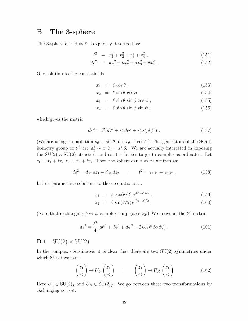
B The 3-sphere

The 3-sphere of radius ℓ is explicitly described as:

ℓ2 = x21 + x2

2 + x23 + x2

4 , (151)

ds2 = dx21 + dx2

2 + dx23 + dx2

4 . (152)

One solution to the constraint is

x1 = ℓ cos θ , (153)

x2 = ℓ sin θ cos φ , (154)

x3 = ℓ sin θ sin φ cosψ , (155)

x4 = ℓ sin θ sin φ sinψ , (156)

which gives the metric

ds2 = ℓ2(dθ2 + s2θ dφ

2 + s2θ s

2φ dψ

2) . (157)

(We are using the notation sθ ≡ sin θ and cθ ≡ cos θ.) The generators of the SO(4)

isometry group of S3 are Λij ∼ xi ∂j − xj ∂i. We are actually interested in exposing

the SU(2) × SU(2) structure and so it is better to go to complex coordinates. Let

z1 = x1 + ix2 z2 = x3 + ix4. Then the sphere can also be written as:

ds2 = dz1 dz1 + dz2 dz2 ; ℓ2 = z1 z1 + z2 z2 . (158)

Let us parametrize solutions to these equations as:

z1 = ℓ cos(θ/2) ei(φ+ψ)/2 , (159)

z2 = ℓ sin(θ/2) ei(φ−ψ)/2 . (160)

(Note that exchanging φ↔ ψ complex conjugates z2.) We arrive at the S3 metric

ds2 =ℓ2

4[dθ2 + dφ2 + dψ2 + 2 cos θ dφ dψ] . (161)

B.1 SU(2) × SU(2)

In the complex coordinates, it is clear that there are two SU(2) symmetries under

which S3 is invariant:(

z1z2

)

→ UL

(

z1z2

)

;

(

z1z2

)

→ UR

(

z1z2

)

(162)

Here UL ∈ SU(2)L and UR ∈ SU(2)R. We go between these two transformations by

exchanging φ↔ ψ.

32

We can compute the action of SU(2)L explicitly. Write the group elements as

UL = e−θi Ti in terms of generators

T1 = − i

2

(

0 1

1 0

)

; T2 =1

2

(

0 −1

1 0

)

; T3 = − i

2

(

1 0

0 −1

)

. (163)

With a little labour one can show that the infinitesimal transformations are explicitly

realized on (z1, z2) by the differential operators

L1 = cψ ∂θ +sψsθ∂φ − sψ cot θ ∂ψ , (164)

L2 = −sψ ∂θ +cψsθ∂φ − cψ cot θ ∂ψ , (165)

L3 = ∂ψ . (166)

Since the exchange (φ ↔ ψ) exchanges SU(2)L and SU(2)R, the SU(2)R transforma-

tions are explicitly realized by the differential operators

R1 = cφ ∂θ +sφsθ∂ψ − sφ cot θ ∂φ , (167)

R2 = −sφ ∂θ +cφsθ∂ψ − cφ cot θ ∂φ , (168)

R3 = ∂φ . (169)

It is also easy to check explicitly that these operators obey the Lie algebra of SU(2)×SU(2):

[Li,Lj] = ǫijk Lk ; [Ri′,Rj′] = ǫi′j′k′ Rk′ ; [Li,Rj′] = 0 . (170)

The indices i and i′ on Li and Ri′ can be raised and lowered freely.

B.2 Killing vectors and vielbeins

S3 has six Killing vectors, which can be taken to be the generators of the SU(2)L and

SU(2)R symmetries above. That is,

KmI = Lm

I I = 1, 2, 3 , (171)

= RmI−3 I = 4, 5, 6 . (172)

The corresponding one-forms have components

L1m =ℓ2

4(cψ, sψ sθ, 0) , (173)

L2m =ℓ2

4(−sψ, cψ sθ, 0) , (174)

L3m =ℓ2

4(0, cθ, 1) , (175)

33

R1m =ℓ2

4(cφ, 0, sφ sθ) , (176)

R2m =ℓ2

4(−sφ, 0, cφ sθ) , (177)

R3m =ℓ2

4(0, 1, cθ) . (178)

There are also two choices of vielbein for S3 constructed from the SU(2)L and

SU(2)R generators. A vielbein is defined by

eam ebn δab = gmn , (179)

eam ebn g

mn = δab . (180)

The norm of the one-forms above is

Lim Ljn gmn = δij

ℓ2

4; Ri′mRj′n g

mn = δi′j′ℓ2

4. (181)

Since the sphere is 3-dimensional, the L and R cannot of course be mutually orthog-

onal as vectors. It is readily checked that

Lim Ljn δij = gmn

ℓ2

4, (182)

and similarly for R. Thus, we can construct a vielbein by identifying the group index

i with a tangent index a and introducing an appropriate normalization factor. The

left and right vielbeins defined in this manner are:

eLam =2

ℓLam ; eRa′m = −2

ℓRa′m . (183)

B.3 Volumes

In these Euler angle coordinates, the volume of the sphere is

Vol =∫ π

0dθ

∫ 2π

0dφ

∫ 4π

0dψ

√

det g =∫ π

0dθ

∫ 2π

0dφ

∫ 4π

0dψ

(

ℓ

2

)3

sin θ = ℓ3 2π2 .

(184)

Accordingly, the volume form for S3 is

(

ℓ

2

)3

sin θ dθ ∧ dφ ∧ dψ ≡ V ǫmnrdxmdxndxr. (185)

B.4 Computing NIr and the SU(2) projectors

The discussion of the consistent ansatz for the three-form involved a two-form

ω = V ǫmnrKmI dx

n dxr , (186)

34

which is closed, and hence, on the sphere, an exact form. So we can write

ω = d(NIrdxr) = ∂nNIr dx

n ∧ dxr (187)

for some NIr. That is, NIr are defined as the solutions of

∂nNIr − ∂rNIn = 2V ǫmnrKmI . (188)

It is easy to show that a solution is 11

I = 1, 2, 3 =⇒ NIm = −ℓKIm , (189)

I = 4, 5, 6 =⇒ NIm = ℓKIm . (190)

The defining equation (188) then implies

∂nKIr − ∂rKIn =2V

ℓ2ǫmnrN

mI . (191)

We can rewrite this with tangent indices by contracting with the vielbein ema , yielding

∂aKIb − ∂bKIa =2

ℓ2ǫabcN

cI . (192)

Taken together with the fact that KI are Killing vectors, this implies

∇aKIb =1

ℓ2ǫabcN

cI . (193)

We can construct the combinations:

RIr = −NIr

ℓ−KIm ; LIr = −NIr

ℓ+ KIm . (194)

Clearly,

RIr = 0 I = 1, 2, 3 , (195)

= −2KIm = −2R(I−3)m I = 4, 5, 6 , (196)

and

LIr = 2KIm = 2LIm I = 1, 2, 3 , (197)

= 0 I = 1, 2, 3 . (198)

Thus, these combinations act as projectors onto SU(2)L and SU(2)R respectively. In

the Killing spinor equations, these projectors appear with flat tangent indices, i.e.,

11We can of course add any closed one-form to NIr and we will still have a solution; we will always

choose to use the above solution.

35

LIa = LImema and RIa = RIme

ma where ema is a left or right vielbein. Recalling the

expressions for the vielbeins given in (183),

RIr = 0 I = 1, 2, 3 , (199)

= ℓeR(I−3)m I = 4, 5, 6 , (200)

and

LIr = ℓeLIm I = 1, 2, 3 , (201)

= 0 I = 1, 2, 3 . (202)

Since the SU(2)L and SU(2)R equations decouple, we can go to a tangent frame using

eL and eR separately in each case. So, choosing the left and right tangent frames in

each case (call the indices a and a′), we find:

RIa′ = 0 I = 1, 2, 3 , (203)

= ℓδ(I−3)a′ I = 4, 5, 6 , (204)

and

LIa = ℓδIa I = 1, 2, 3 , (205)

= 0 I = 1, 2, 3 . (206)

References

[1] S. W. Hawking, “Particle creation by black holes,” Commun. Math. Phys. 43,

199 (1975).

[2] M. Banados, C. Teitelboim and J. Zanelli, “The black hole in three-dimensional

space-time,” Phys. Rev. Lett. 69, 1849 (1992) [hep-th/9204099]; M. Banados,

M. Henneaux, C. Teitelboim and J. Zanelli, “Geometry of the (2+1) black hole,”

Phys. Rev. D 48, 1506 (1993) [gr-qc/9302012].

[3] S. Deser, R. Jackiw and G. ’t Hooft, “Three-dimensional Einstein gravity: dy-

namics of flat space,” Annals Phys. 152, 220 (1984); S. Deser and R. Jackiw,

“Three-dimensional cosmological gravity: dynamics of constant curvature,” An-

nals Phys. 153 (1984) 405.

[4] H. Matschull, “Black hole creation in 2 + 1-dimensions,” Class. Quant. Grav.

16, 1069 (1999) [gr-qc/9809087]. A. R. Steif, “Time-symmetric initial data for

multi-body solutions in three dimensions,” Phys. Rev. D 53, 5527 (1996) [gr-

qc/9511053].

36

[5] J. Maldacena, “The large N limit of superconformal field theories and supergrav-

ity,” Adv. Theor. Math. Phys. 2, 231 (1998) [hep-th/9711200].

[6] V. Balasubramanian and S. F. Ross, “Holographic particle detection,” Phys.

Rev. D 61, 044007 (2000) [hep-th/9906226].

[7] U. H. Danielsson, E. Keski-Vakkuri and M. Kruczenski, “Black hole formation

in AdS and thermalization on the boundary,” JHEP 0002, 039 (2000) [hep-

th/9912209]; U. H. Danielsson, E. Keski-Vakkuri and M. Kruczenski, “Spher-

ically collapsing matter in AdS, holography, and shellons,” Nucl. Phys. B563,

279 (1999) [hep-th/9905227].

[8] J. M. Izquierdo and P. K. Townsend, “Supersymmetric space-times in (2 + 1)

AdS supergravity models,” Class. Quant. Grav. 12, 895 (1995) [gr-qc/9501018].

[9] J. R. David, G. Mandal, S. Vaidya and S. R. Wadia, “Point mass geometries,

spectral flow and AdS3-CFT2 correspondence,” Nucl. Phys. B564, 128 (2000)

[hep-th/9906112].

[10] M. J. Duff, B. E. Nilsson and C. N. Pope, “Kaluza-Klein supergravity,” Phys.

Rept. 130, 1 (1986).

[11] M. Cvetic, H. Lu and C. N. Pope, “Consistent Kaluza-Klein sphere reductions,”

Phys. Rev. D 62, 064028 (2000) [hep-th/0003286]; M. Cvetic, H. Lu,

C. N. Pope, A. Sadrzadeh and T. A. Tran, “S(3) and S(4) reductions of type IIA

supergravity,” Nucl. Phys. B590, 233 (2000) [hep-th/0005137].

[12] A. Strominger, “Black hole entropy from near-horizon microstates,” JHEP 9802,

009 (1998) [hep-th/9712251]; D. Birmingham, I. Sachs and S. Sen, “Entropy of

three-dimensional black holes in string theory,” Phys. Lett. B424, 275 (1998)

[hep-th/9801019].

[13] A. Strominger and C. Vafa, “Microscopic origin of the Bekenstein-Hawking en-

tropy,” Phys. Lett. B379, 99 (1996) [hep-th/9601029].

[14] V. Balasubramanian and F. Larsen, “Near horizon geometry and black holes in

four dimensions,” Nucl. Phys. B528, 229 (1998) [hep-th/9802198].

[15] F. Larsen and E. Martinec, “U(1) charges and moduli in the D1-D5 system,”

JHEP 9906, 019 (1999) [hep-th/9905064]; R. Dijkgraaf, “Instanton strings

and hyperKaehler geometry,” Nucl. Phys. B543, 545 (1999) [hep-th/9810210].

[16] V. Balasubramanian and P. Kraus, “A stress tensor for anti-de Sitter gravity,”

Commun. Math. Phys. 208, 413 (1999) [hep-th/9902121].

37

[17] L. F. Abbott and S. Deser, “Stability of gravity with a cosmological constant,”

Nucl. Phys. B195, 76 (1982); S. W. Hawking and G. T. Horowitz, “The grav-

itational Hamiltonian, action, entropy and surface terms,” Class. Quant. Grav.

13, 1487 (1996) [gr-qc/9501014].

[18] L. J. Romans, “Selfduality for interacting fields: covariant field equations for

six-dimensional chiral supergravities,” Nucl. Phys. B276, 71 (1986).

[19] S. Deger, A. Kaya, E. Sezgin and P. Sundell, “Spectrum of D = 6, N = 4b

supergravity on AdS3 × S3,” Nucl. Phys. B536, 110 (1998) [hep-th/9804166].

[20] F. Larsen, “The perturbation spectrum of black holes in N = 8 supergravity,”

Nucl. Phys. B536, 258 (1998) [hep-th/9805208].

[21] J. de Boer, “Six-dimensional supergravity on S3 × AdS3 and 2d conformal field

theory,” Nucl. Phys. B548, 139 (1999) [hep-th/9806104].

[22] A. Achucarro and P. K. Townsend, “Extended supergravities in D = (2 + 1) as

Chern-Simons theories,” Phys. Lett. B229, 383 (1989).

[23] E. J. Martinec, “Matrix models of AdS gravity,” hep-th/9804111.

[24] M. Nishimura and Y. Tanii, “Super Weyl anomalies in the AdS/CFT correspon-

dence,” Int. J. Mod. Phys. A14, 3731 (1999) [hep-th/9904010].

[25] J. R. David, “Anti-de Sitter gravity associated with the supergroup SU(1, 1|2)×SU(1, 1|2),” Mod. Phys. Lett. A14, 1143 (1999) [hep-th/9904068].

[26] M. Asorey, F. Falceto and S. Carlip, “Chern-Simons states and topologically

massive gauge theories,” Phys. Lett. B312, 477 (1993) [hep-th/9304081].

[27] G. Arutyunov, A. Pankiewicz and S. Theisen, “Cubic couplings in D = 6 N =

4b supergravity on AdS(3) x S**3,” hep-th/0007061.

[28] O. Coussaert and M. Henneaux, “Supersymmetry of the (2+1) black holes,”

Phys. Rev. Lett. 72, 183 (1994) [hep-th/9310194].

[29] M. Cvetic and D. Youm, “Rotating intersecting M-branes,” Nucl. Phys. B499,

253 (1997) [hep-th/9612229].

[30] M. Cvetic and F. Larsen, “Near horizon geometry of rotating black holes in five

dimensions,” Nucl. Phys. B531, 239 (1998) [hep-th/9805097].

[31] J. C. Breckenridge, R. C. Myers, A. W. Peet and C. Vafa, “D-branes and spinning

black holes,” Phys. Lett. B391, 93 (1997) [hep-th/9602065].

38

[32] A. W. Peet and S. F. Ross, “Microcanonical phases of string theory on AdSm ×Sn,” JHEP 9812, 020 (1998) [hep-th/9810200].

[33] R. Gregory and R. Laflamme, “Black strings and p-branes are unstable,” Phys.

Rev. Lett. 70, 2837 (1993) [hep-th/9301052]; R. Gregory and R. Laflamme,

“The Instability of charged black strings and p-branes,” Nucl. Phys. B428, 399

(1994) [hep-th/9404071].

[34] V. Balasubramanian, J. de Boer, E. Keski-Vakkuri and S.F. Ross, in preparation.

[35] O. Coussaert, M. Henneaux and P. van Driel, “The Asymptotic dynamics of

three-dimensional Einstein gravity with a negative cosmological constant,” Class.

Quant. Grav. 12, 2961 (1995) [gr-qc/9506019].

[36] M. Banados, K. Bautier, O. Coussaert, M. Henneaux and M. Ortiz, “Anti-de

Sitter/CFT correspondence in three-dimensional supergravity,” Phys. Rev. D58,

085020 (1998) [hep-th/9805165].

[37] M. Henneaux, L. Maoz and A. Schwimmer, “Asymptotic dynamics and asymp-

totic symmetries of three-dimensional extended AdS supergravity,” Annals Phys.

282, 31 (2000) [hep-th/9910013].

[38] A. Schwimmer and N. Seiberg, “Comments on The N=2, N=3, N=4 superconfor-

mal algebras in two-dimensions,” Phys. Lett. B184, 191 (1987); M. Yu, “The

unitary constructions of the N = 4 SU(2) extended superconformal algebras,”

Phys. Lett. B196, 345 (1987).

[39] E. Martinec and V. Sahakian, “Black holes and five-brane thermodynamics,”

Phys. Rev. D60, 064002 (1999) [hep-th/9901135].

[40] J. Cho and S. Nam, “AdS(3) black hole entropy and the spectral flow on the

horizon,” hep-th/9903058.

[41] We learned this from R.T. Griffiths, “Internet for historians, his-

tory of the Internet e-mail, newsgroups and lists”, a web page at

www.let.leidenuniv.nl/history/ivh/INTERNET2.htm♯ 1 .

[42] T. Kugo and P. Townsend, “Supersymmetry and the division algebras,” Nucl.

Phys. B221, 357 (1983).

[43] P. S. Howe, G. Sierra and P. K. Townsend, “Supersymmetry in six-dimensions,”

Nucl. Phys. B221, 331 (1983).

39