Spectrum of the open QCD flux tube and its effective string ...
54
Spectrum of the open QCD flux tube and its effective string description Spectrum of the open QCD flux tube and its effective string description Bastian Brandt ITP Goethe-Universit¨ at Frankfurt 02.06.2018
-
Upload
khangminh22 -
Category
Documents
-
view
0 -
download
0
Transcript of Spectrum of the open QCD flux tube and its effective string ...
Spectrum of the open QCD flux tube and its effective string description
Spectrum of the open QCD flux tube and itseffective string description
Bastian Brandt
ITP Goethe-Universitat Frankfurt
02.06.2018
Spectrum of the open QCD flux tube and its effective string description
Contents
1. IntroductionConfinement, flux tubes and strings
2. String tension and KKN prediction
3. EST analysis without massive modes
4. Testing the presence of massive modes
5. Conclusions
Spectrum of the open QCD flux tube and its effective string description
Introduction
1. Introduction
Confinement, flux tubes and strings
Spectrum of the open QCD flux tube and its effective string description
Introduction
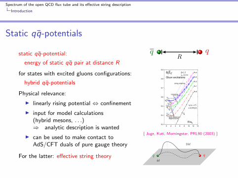
Static qq-potentials
static qq-potential:
energy of static qq pair at distance R
for states with excited gluons configurations:
hybrid qq-potentials
Physical relevance:
I linearly rising potential ⇔ confinement
I input for model calculations(hybrid mesons, . . .)⇒ analytic description is wanted
I can be used to make contact toAdS/CFT duals of pure gauge theory
For the latter: effective string theory
Rqq
0.3
0.4
0.5
0.6
0.7
0.8
0.9
0 2 4 6 8 10 12 14
atEΓ
R/as
Gluon excitations
as/at = z*5
z=0.976(21)
β=2.5as~0.2 fm
Πu
Σ-u
Σ+g’
∆gΠg
Σ-g
Πg’Π’u
Σ+u
∆u
Σ+g
short distancedegeneracies
crossover
string ordering
N=4
N=3
N=2
N=1
N=0
[ Juge, Kuti, Morningstar, PRL90 (2003) ]
10d
4d

Spectrum of the open QCD flux tube and its effective string description
Introduction
Confinement and flux tubes
Heuristic confinement mechanism:
I qq pair connected by region of strongchromo-electromagnetic flux
I pulling the quarks appart:flux gets squeezed into a narrow region
⇒ flux tube
I squeezing due to dual Meissner effectI here all quarks are static
(no string breaking)
I for such a tube:expect constant energy density
⇒ linearly rising potential V (R) = σR
σ : string tension
Rqq
Spectrum of the open QCD flux tube and its effective string description
Introduction
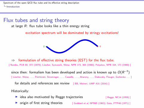
Flux tubes and string theoryat large R: flux tube looks like a thin energy string
excitation spectrum will be dominated by stringy excitations!
⇒ formulation of effective string theories (EST) for the flux tube.[ Nambu, PLB 80, 372 (1979); Luscher, Symanzik, Weisz, NPB 173, 365 (1980); Polyakov, NPB 164, 171 (1980) ]
since then: formalism has been developed and action is known up to O(R−5)[ Luscher, Weisz, . . . , Polchinski, Strominger, . . . , Casselle, . . . , Aharony, . . . , Dubovsky, Flauger, Gorbenko . . . ]
for details and references see review [ BB, Meineri, IJMP A31 (2016) ]
Historically:
I idea also motivated by Regge trajectories [ Regge, NC14 (1959) ]
I origin of first string theories [ Goddard et al, NPB65 (1963); Goto, PTP46 (1971) ]

Spectrum of the open QCD flux tube and its effective string description
Introduction
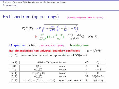
EST spectrum (open strings) [ Aharony, Klinghoffer, JHEP1012 (2010) ]
EESTn,l (R) = σ R
√1 +
2π
σ R2
(n −
1
24(d − 2)
)−b2
π3
√σ3R4
(B ln +
d − 2
60
)−π3(d − 26)
48σ2R5C ln +O(R−ξ)
LC spectrum (or NG) [ J.F. Arvis, PLB127 (1983) ] boundary term
b2: dimensionless non-universal boundary coefficient b2 =√σ3b2
B ln, C
ln: dimensionless, depend on representation of SO(d − 2)
|n, l⟩
SO(d − 2) representation B ln C l
n
|0⟩
1|0⟩
scalar 0 0
|1⟩
αi−1|0
⟩vector 4 d − 3
|2, 1⟩
αi−1α
i−1|0
⟩scalar 8 0
|2, 2⟩
αi−2|0
⟩vector 32 16(d − 3)
|2, 3⟩ (
αi−1α
j−1 −
δij
d−2αi−1α
i−1
)|0⟩
sym. tracel. tensor 8 4(d − 2)
Spectrum of the open QCD flux tube and its effective string description
Introduction
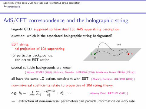
AdS/CFT correspondence and the holographic string
large-N QCD: supposed to have dual 10d AdS superstring description
question: which is the associated holographic string background?
EST string:4d projection of 10d superstring
for particular backgrounds:can derive EST action
10d
4d
several suitable backgrounds are known[ Witten, ATMP2 (1998); Klebanov, Strassler, JHEP0008 (2000); Maldacena, Nunez, PRL86 (2001) ]
all have the same LO action, consistent with EST [ Aharony, Karzbrun, JHEP0906 (2009) ]
non-universal coefficients relate to properties of 10d string theory
e.g. b2 = − 164σ
∑ξ
(−1)BC(ξ)
mbξ
+ bf2 + . . . [ Aharony, Field, JHEP1101 (2011) ]
⇒ extraction of non-universal parameters can provide information on AdS side

Spectrum of the open QCD flux tube and its effective string description
Introduction
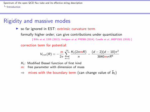
Rigidity and massive modesI so far ignored in EST: extrinsic curvature term
formally higher order; can give contributions under quantisation[ Billo et al, 1205 (2012); Ambjorn et al, PRD89 (2014); Caselle et al, JHEP1501 (2015) ]
correction term for potential:
Vext(R) = −m
2π
∞∑n=1
K1(2nmR)
n−
(d − 2)(d − 10)π2
3840mσR4
K1: Modified Bessel function of first kindm: free parameter with dimension of mass
⇒ mixes with the boundary term (can change value of b2)
I other possible contribution: massive modes
found to be important to describe 4d spectrum[ Dubovsky, Flauger, Gorbenko, PRL111 (2013); JETP120 (2015) ]
however: 4d coupling term not allowed in 3d
can only couple indirectly via the induced metric
⇒ formally similar contribution to rigidity term!
Spectrum of the open QCD flux tube and its effective string description
Introduction
Rigidity and massive modesI so far ignored in EST: extrinsic curvature term
formally higher order; can give contributions under quantisation[ Billo et al, 1205 (2012); Ambjorn et al, PRD89 (2014); Caselle et al, JHEP1501 (2015) ]
correction term for potential:
Vext(R) = −m
2π
∞∑n=1
K1(2nmR)
n−
(d − 2)(d − 10)π2
3840mσR4
K1: Modified Bessel function of first kindm: free parameter with dimension of mass
⇒ mixes with the boundary term (can change value of b2)
I other possible contribution: massive modes
found to be important to describe 4d spectrum[ Dubovsky, Flauger, Gorbenko, PRL111 (2013); JETP120 (2015) ]
however: 4d coupling term not allowed in 3d
can only couple indirectly via the induced metric
⇒ formally similar contribution to rigidity term!
Spectrum of the open QCD flux tube and its effective string description
Introduction
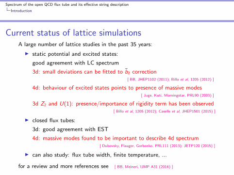
Current status of lattice simulationsA large number of lattice studies in the past 35 years:
I static potential and excited states:
good agreement with LC spectrum
3d: small deviations can be fitted to b2 correction[ BB, JHEP1102 (2011); Billo et al, 1205 (2012) ]
4d: behaviour of excited states points to presence of massive modes[ Juge, Kuti, Morningstar, PRL90 (2003) ]
3d Z2 and U(1): presence/importance of rigidity term has been observed[ Billo et al, 1205 (2012); Caselle et al, JHEP1501 (2015) ]
I closed flux tubes:
3d: good agreement with EST
4d: massive modes found to be important to describe 4d spectrum[ Dubovsky, Flauger, Gorbenko, PRL111 (2013); JETP120 (2015) ]
I can also study: flux tube width, finite temperature, ...
for a review and more references see [ BB, Meineri, IJMP A31 (2016) ]

Spectrum of the open QCD flux tube and its effective string description
Introduction
Goals and setup of this study
first goal: extract EST parameters at finite N and in the N →∞ limit
in particular: use pure gauge lattice simulation in 3d
I extract√σr0 and b2 in 3d SU(N = 2, 3, 4, 5, 6) from V (R)
I multiple lattice spacings a ≈ 0.11, 0.08, 0.06 fm with V & 5 fmI error reduction: LW algorithm
(2000 total meas; 20 000 sub. updates; ts = 2, 4, 6)
I extrapolate to continuum a→ 0 and subsequently N →∞.
I check the consistency of results with the excited states
here: use old SU(2) data from [ BB, JHEP1102 (2011) ]
second goal: test consistency with massive modes/string rigidity
I extract mass m and investigate impact on b2
I once more: compare continuum results for different values of N
⇒ extrapolate N →∞?
Spectrum of the open QCD flux tube and its effective string description
String tension and KKN prediction
2. String tension and KKN prediction
Spectrum of the open QCD flux tube and its effective string description
String tension and KKN prediction
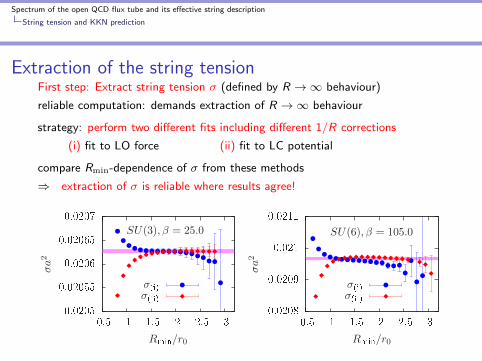
Extraction of the string tensionFirst step: Extract string tension σ (defined by R →∞ behaviour)
reliable computation: demands extraction of R →∞ behaviour
strategy: perform two different fits including different 1/R corrections
(i) fit to LO force (ii) fit to LC potential
compare Rmin-dependence of σ from these methods
⇒ extraction of σ is reliable where results agree!
0.0205
0.02055
0.0206
0.02065
0.0207
0.5 1 1.5 2 2.5 3
σa2
Rmin
/r0
SU(3), β = 25.0
0.0208
0.0209
0.021
0.0211
0.5 1 1.5 2 2.5 3
σa2
Rmin
/r0
SU(6), β = 105.0
σ(i)
σ(ii)
σ(i)
σ(ii)
Spectrum of the open QCD flux tube and its effective string description
String tension and KKN prediction
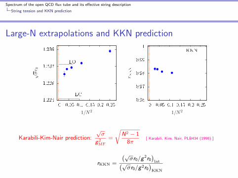
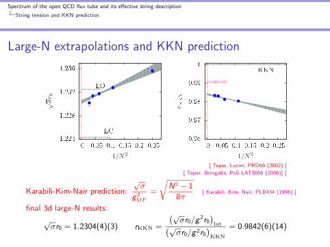
Large-N extrapolations and KKN prediction
1.224
1.228
1.232
1.236
0 0.05 0.1 0.15 0.2 0.25
√σr 0
1/N2
LO
LC
0.96
0.97
0.98
0.99
1
0 0.05 0.1 0.15 0.2 0.25
r KK
N
1/N2
KKN
[ Teper, Lucini, PRD66 (2002) ]
[ Teper, Bringoltz, PoS LAT2006 (2006)] ]
Karabili-Kim-Nair prediction:
√σ
g 2MF
=
√N2 − 1
8π[ Karabili, Kim, Nair, PLB434 (1998) ]
final 3d large-N results:
√σr0 = 1.2304(4)(3)
rKKN =
(√σr0/g
2r0
)lat(√
σr0/g 2r0
)KKN
= 0.9842(6)(14)
Spectrum of the open QCD flux tube and its effective string description
String tension and KKN prediction
Large-N extrapolations and KKN prediction
1.224
1.228
1.232
1.236
0 0.05 0.1 0.15 0.2 0.25
√σr 0
1/N2
LO
LC
0.96
0.97
0.98
0.99
1
0 0.05 0.1 0.15 0.2 0.25
r KK
N
1/N2
KKN
[ Teper, Lucini, PRD66 (2002) ]
[ Teper, Bringoltz, PoS LAT2006 (2006)] ]
Karabili-Kim-Nair prediction:
√σ
g 2MF
=
√N2 − 1
8π[ Karabili, Kim, Nair, PLB434 (1998) ]
final 3d large-N results:
√σr0 = 1.2304(4)(3) rKKN =
(√σr0/g
2r0
)lat(√
σr0/g 2r0
)KKN
= 0.9842(6)(14)

Spectrum of the open QCD flux tube and its effective string description
EST analysis without massive modes
3. EST analysis without massive modes

Spectrum of the open QCD flux tube and its effective string description
EST analysis without massive modes
Order of the leading order correction
first: check consistency of correction to LC potential with R−4
fit V (R) to form: V (R) = ELC0 (R) +
η(√σR)m
look at Rmin dependence of m:
0
2
4
6
8
10
0 0.6 1.2 1.8
m
R/r0
SU(3)
0
2
4
6
8
10
0 0.6 1.2 1.8
m
R/r0
SU(5)
β = 31.0 β = 71.0
Spectrum of the open QCD flux tube and its effective string description
EST analysis without massive modes
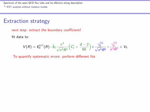
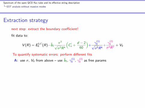
Extraction strategy
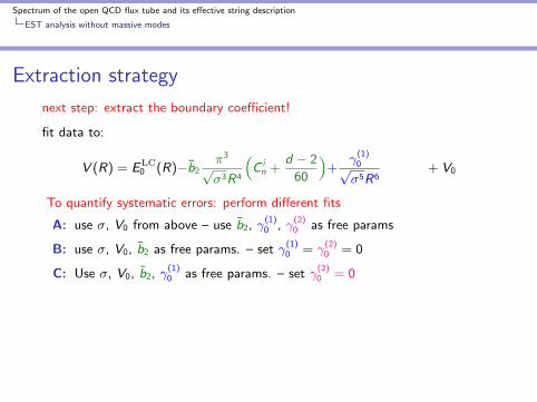
next step: extract the boundary coefficient!
fit data to:
V (R) = ELC0 (R)−b2
π3
√σ3R4
(C in +
d − 2
60
)+
γ(1)0√σ5R6
+γ
(2)0
σ3R7+ V0
To quantify systematic errors: perform different fits
A: use σ, V0 from above – use b2, γ(1)0 , γ
(2)0 as free params
B: use σ, V0, b2 as free params. – set γ(1)0 = γ
(2)0 = 0
C: Use σ, V0, b2, γ(1)0 as free params. – set γ
(2)0 = 0
D: Use σ, V0, b2, γ(2)0 as free params. – set γ
(1)0 = 0
E: Use σ, V0, γ(1)0 , γ
(2)0 as free params. – set b2 = 0
fits A and E are checks whether b2 6= 0
fits B–D are used in the final analysis
Spectrum of the open QCD flux tube and its effective string description
EST analysis without massive modes
Extraction strategy
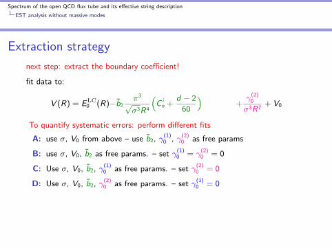
next step: extract the boundary coefficient!
fit data to:
V (R) = ELC0 (R)−b2
π3
√σ3R4
(C in +
d − 2
60
)+
γ(1)0√σ5R6
+γ
(2)0
σ3R7+ V0
To quantify systematic errors: perform different fits
A: use σ, V0 from above – use b2, γ(1)0 , γ
(2)0 as free params
B: use σ, V0, b2 as free params. – set γ(1)0 = γ
(2)0 = 0
C: Use σ, V0, b2, γ(1)0 as free params. – set γ
(2)0 = 0
D: Use σ, V0, b2, γ(2)0 as free params. – set γ
(1)0 = 0
E: Use σ, V0, γ(1)0 , γ
(2)0 as free params. – set b2 = 0
fits A and E are checks whether b2 6= 0
fits B–D are used in the final analysis
Spectrum of the open QCD flux tube and its effective string description
EST analysis without massive modes
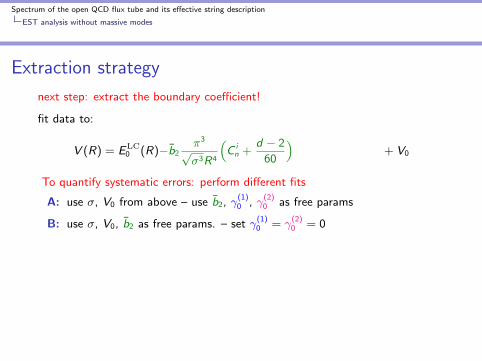
Extraction strategy
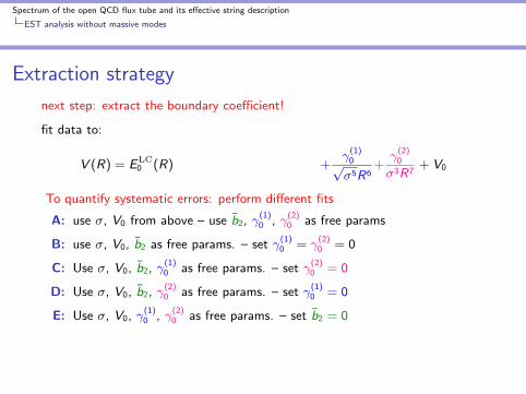
next step: extract the boundary coefficient!
fit data to:
V (R) = ELC0 (R)−b2
π3
√σ3R4
(C in +
d − 2
60
)
+γ
(1)0√σ5R6
+γ
(2)0
σ3R7
+ V0
To quantify systematic errors: perform different fits
A: use σ, V0 from above – use b2, γ(1)0 , γ
(2)0 as free params
B: use σ, V0, b2 as free params. – set γ(1)0 = γ
(2)0 = 0
C: Use σ, V0, b2, γ(1)0 as free params. – set γ
(2)0 = 0
D: Use σ, V0, b2, γ(2)0 as free params. – set γ
(1)0 = 0
E: Use σ, V0, γ(1)0 , γ
(2)0 as free params. – set b2 = 0
fits A and E are checks whether b2 6= 0
fits B–D are used in the final analysis
Spectrum of the open QCD flux tube and its effective string description
EST analysis without massive modes
Extraction strategy
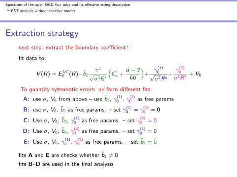
next step: extract the boundary coefficient!
fit data to:
V (R) = ELC0 (R)−b2
π3
√σ3R4
(C in +
d − 2
60
)+
γ(1)0√σ5R6
+γ
(2)0
σ3R7
+ V0
To quantify systematic errors: perform different fits
A: use σ, V0 from above – use b2, γ(1)0 , γ
(2)0 as free params
B: use σ, V0, b2 as free params. – set γ(1)0 = γ
(2)0 = 0
C: Use σ, V0, b2, γ(1)0 as free params. – set γ
(2)0 = 0
D: Use σ, V0, b2, γ(2)0 as free params. – set γ
(1)0 = 0
E: Use σ, V0, γ(1)0 , γ
(2)0 as free params. – set b2 = 0
fits A and E are checks whether b2 6= 0
fits B–D are used in the final analysis
Spectrum of the open QCD flux tube and its effective string description
EST analysis without massive modes
Extraction strategy
next step: extract the boundary coefficient!
fit data to:
V (R) = ELC0 (R)−b2
π3
√σ3R4
(C in +
d − 2
60
)
+γ
(1)0√σ5R6
+γ
(2)0
σ3R7+ V0
To quantify systematic errors: perform different fits
A: use σ, V0 from above – use b2, γ(1)0 , γ
(2)0 as free params
B: use σ, V0, b2 as free params. – set γ(1)0 = γ
(2)0 = 0
C: Use σ, V0, b2, γ(1)0 as free params. – set γ
(2)0 = 0
D: Use σ, V0, b2, γ(2)0 as free params. – set γ
(1)0 = 0
E: Use σ, V0, γ(1)0 , γ
(2)0 as free params. – set b2 = 0
fits A and E are checks whether b2 6= 0
fits B–D are used in the final analysis
Spectrum of the open QCD flux tube and its effective string description
EST analysis without massive modes
Extraction strategy
next step: extract the boundary coefficient!
fit data to:
V (R) = ELC0 (R)
−b2π3
√σ3R4
(C in +
d − 2
60
)
+γ
(1)0√σ5R6
+γ
(2)0
σ3R7+ V0
To quantify systematic errors: perform different fits
A: use σ, V0 from above – use b2, γ(1)0 , γ
(2)0 as free params
B: use σ, V0, b2 as free params. – set γ(1)0 = γ
(2)0 = 0
C: Use σ, V0, b2, γ(1)0 as free params. – set γ
(2)0 = 0
D: Use σ, V0, b2, γ(2)0 as free params. – set γ
(1)0 = 0
E: Use σ, V0, γ(1)0 , γ
(2)0 as free params. – set b2 = 0
fits A and E are checks whether b2 6= 0
fits B–D are used in the final analysis
Spectrum of the open QCD flux tube and its effective string description
EST analysis without massive modes
Extraction strategy
next step: extract the boundary coefficient!
fit data to:
V (R) = ELC0 (R)−b2
π3
√σ3R4
(C in +
d − 2
60
)+
γ(1)0√σ5R6
+γ
(2)0
σ3R7+ V0
To quantify systematic errors: perform different fits
A: use σ, V0 from above – use b2, γ(1)0 , γ
(2)0 as free params
B: use σ, V0, b2 as free params. – set γ(1)0 = γ
(2)0 = 0
C: Use σ, V0, b2, γ(1)0 as free params. – set γ
(2)0 = 0
D: Use σ, V0, b2, γ(2)0 as free params. – set γ
(1)0 = 0
E: Use σ, V0, γ(1)0 , γ
(2)0 as free params. – set b2 = 0
fits A and E are checks whether b2 6= 0
fits B–D are used in the final analysis

Spectrum of the open QCD flux tube and its effective string description
EST analysis without massive modes
Extraction, limites and estimation of systematic errors
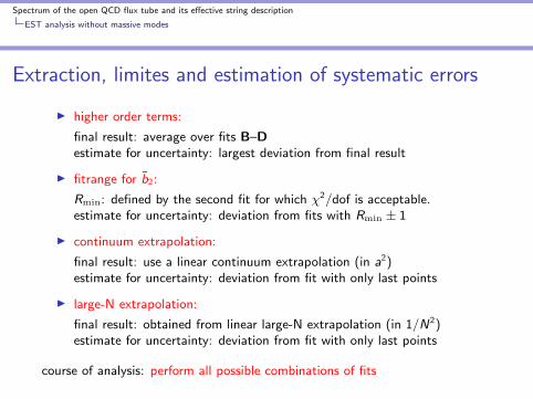
I higher order terms:
final result: average over fits B–Destimate for uncertainty: largest deviation from final result
I fitrange for b2:
Rmin: defined by the second fit for which χ2/dof is acceptable.estimate for uncertainty: deviation from fits with Rmin ± 1
I continuum extrapolation:
final result: use a linear continuum extrapolation (in a2)estimate for uncertainty: deviation from fit with only last points
I large-N extrapolation:
final result: obtained from linear large-N extrapolation (in 1/N2)estimate for uncertainty: deviation from fit with only last points
course of analysis: perform all possible combinations of fits
Spectrum of the open QCD flux tube and its effective string description
EST analysis without massive modes
Extraction, limites and estimation of systematic errors
I higher order terms:
final result: average over fits B–Destimate for uncertainty: largest deviation from final result
I fitrange for b2:
Rmin: defined by the second fit for which χ2/dof is acceptable.estimate for uncertainty: deviation from fits with Rmin ± 1
I continuum extrapolation:
final result: use a linear continuum extrapolation (in a2)estimate for uncertainty: deviation from fit with only last points
I large-N extrapolation:
final result: obtained from linear large-N extrapolation (in 1/N2)estimate for uncertainty: deviation from fit with only last points
course of analysis: perform all possible combinations of fits
Spectrum of the open QCD flux tube and its effective string description
EST analysis without massive modes
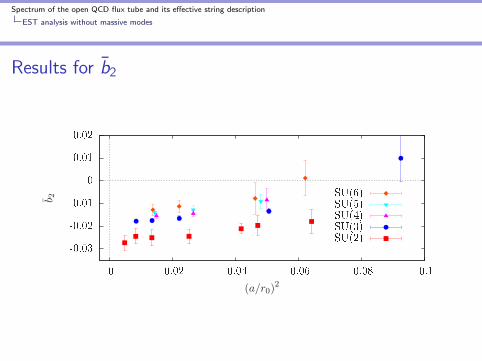
Results for b2
-0.03
-0.02
-0.01
0
0.01
0.02
0 0.02 0.04 0.06 0.08 0.1
b 2
(a/r0)2
SU(6)
SU(5)
SU(4)
SU(3)
SU(2)
Spectrum of the open QCD flux tube and its effective string description
EST analysis without massive modes
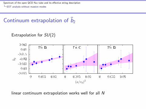
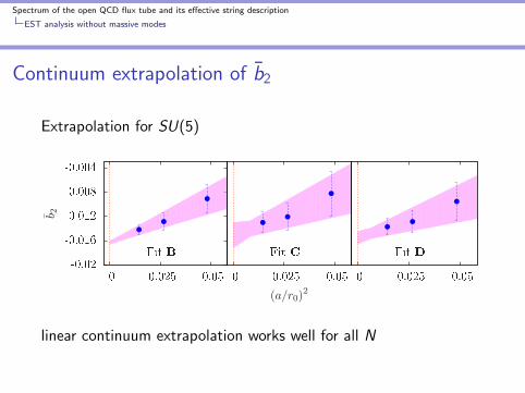
Continuum extrapolation of b2
Extrapolation for SU(2)
-0.035
-0.03
-0.025
-0.02
-0.015
-0.01
-0.005
0 0.025 0.05
b 2
Fit B
0 0.025 0.05
(a/r0)2
Fit C
0 0.025 0.05
Fit D
linear continuum extrapolation works well for all N
Spectrum of the open QCD flux tube and its effective string description
EST analysis without massive modes
Continuum extrapolation of b2
Extrapolation for SU(5)
-0.02
-0.016
-0.012
-0.008
-0.004
0 0.025 0.05
b 2
Fit B
0 0.025 0.05
(a/r0)2
Fit C
0 0.025 0.05
Fit D
linear continuum extrapolation works well for all N
Spectrum of the open QCD flux tube and its effective string description
EST analysis without massive modes
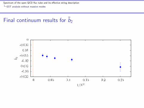
Final continuum results for b2
-0.035
-0.03
-0.025
-0.02
-0.015
-0.01
-0.005
0
0 0.05 0.1 0.15 0.2 0.25
b 2
1/N2
Spectrum of the open QCD flux tube and its effective string description
EST analysis without massive modes
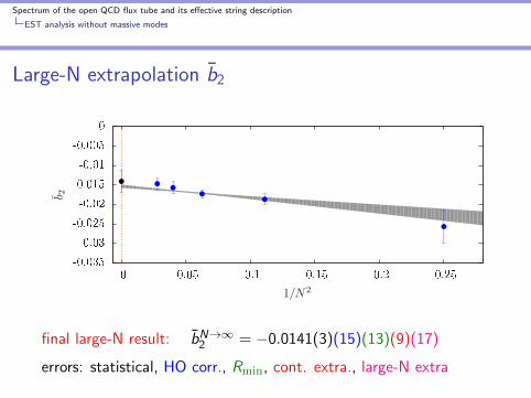
Large-N extrapolation b2
-0.035
-0.03
-0.025
-0.02
-0.015
-0.01
-0.005
0
0 0.05 0.1 0.15 0.2 0.25
b 2
1/N2
final large-N result: bN→∞2 = −0.0141(3)(15)(13)(9)(17)
errors: statistical, HO corr., Rmin, cont. extra., large-N extra
Spectrum of the open QCD flux tube and its effective string description
EST analysis without massive modes
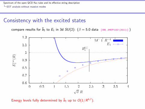
Consistency with the excited states
compare results for b2 to E1 in 3d SU(2): (β = 5.0 data [ BB, JHEP1102 (2011) ] )
0.6
0.7
0.8
0.9
1
1.1
1.2
0 0.5 1 1.5 2 2.5 3 3.5 4
Ersc
1(R
)
√σ R
RLCc
LC + R−4
E1
Energy levels fully determined by b2 up to O(1/R6,7).
Spectrum of the open QCD flux tube and its effective string description
EST analysis without massive modes
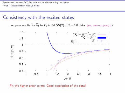
Consistency with the excited states
compare results for b2 to E1 in 3d SU(2): (β = 5.0 data [ BB, JHEP1102 (2011) ] )
0.6
0.7
0.8
0.9
1
1.1
1.2
0 0.5 1 1.5 2 2.5 3 3.5 4
∆E
rsc
10(R
)
√σ R
RLCc
LC + R−4+ R6
LC + R−4
E1
Fit the higher order terms: Good description of the data!
Spectrum of the open QCD flux tube and its effective string description
EST analysis without massive modes
Consistency with the excited states
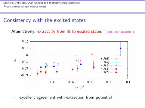
Alternatively: extract b2 from fit to excited states [ BB, JHEP1102 (2011) ]
-0.03
-0.02
-0.01
0
0.01
0.02
0 0.02 0.04 0.06 0.08 0.1
b 2
(a/r0)2
SU(6)
SU(5)
SU(4)
SU(3)
SU(2)
⇒ excellent agreement with extraction from potential
Spectrum of the open QCD flux tube and its effective string description
Testing the presence of massive modes
4. Testing the presence of massive modes
Spectrum of the open QCD flux tube and its effective string description
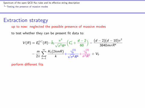
Testing the presence of massive modes
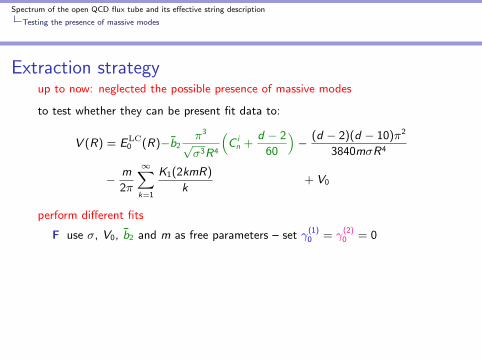
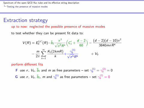
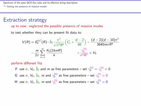
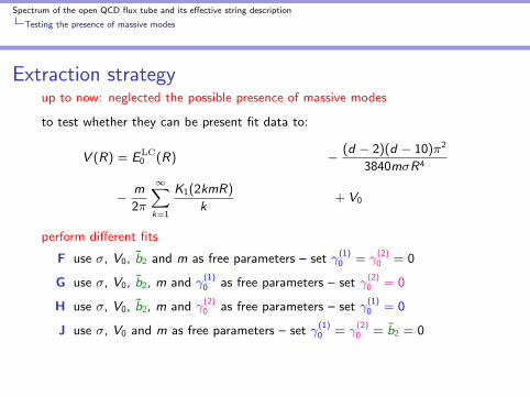
Extraction strategyup to now: neglected the possible presence of massive modes
to test whether they can be present fit data to:
V (R) = ELC0 (R)−b2
π3
√σ3R4
(C in +
d − 2
60
)− (d − 2)(d − 10)π2
3840mσR4
− m
2π
∞∑k=1
K1(2kmR)
k+
γ(1)0√σ5R6
+γ
(2)0
σ3R7+ V0
perform different fits
F use σ, V0, b2 and m as free parameters – set γ(1)0 = γ
(2)0 = 0
G use σ, V0, b2, m and γ(1)0 as free parameters – set γ
(2)0 = 0
H use σ, V0, b2, m and γ(2)0 as free parameters – set γ
(1)0 = 0
J use σ, V0 and m as free parameters – set γ(1)0 = γ
(2)0 = b2 = 0
fit J: check whether b2 6= 0
fit F used in the final analysis (results of G and H not accurate enough)
Spectrum of the open QCD flux tube and its effective string description
Testing the presence of massive modes
Extraction strategyup to now: neglected the possible presence of massive modes
to test whether they can be present fit data to:
V (R) = ELC0 (R)−b2
π3
√σ3R4
(C in +
d − 2
60
)− (d − 2)(d − 10)π2
3840mσR4
− m
2π
∞∑k=1
K1(2kmR)
k
+γ
(1)0√σ5R6
+γ
(2)0
σ3R7
+ V0
perform different fits
F use σ, V0, b2 and m as free parameters – set γ(1)0 = γ
(2)0 = 0
G use σ, V0, b2, m and γ(1)0 as free parameters – set γ
(2)0 = 0
H use σ, V0, b2, m and γ(2)0 as free parameters – set γ
(1)0 = 0
J use σ, V0 and m as free parameters – set γ(1)0 = γ
(2)0 = b2 = 0
fit J: check whether b2 6= 0
fit F used in the final analysis (results of G and H not accurate enough)
Spectrum of the open QCD flux tube and its effective string description
Testing the presence of massive modes
Extraction strategyup to now: neglected the possible presence of massive modes
to test whether they can be present fit data to:
V (R) = ELC0 (R)−b2
π3
√σ3R4
(C in +
d − 2
60
)− (d − 2)(d − 10)π2
3840mσR4
− m
2π
∞∑k=1
K1(2kmR)
k+
γ(1)0√σ5R6
+γ
(2)0
σ3R7
+ V0
perform different fits
F use σ, V0, b2 and m as free parameters – set γ(1)0 = γ
(2)0 = 0
G use σ, V0, b2, m and γ(1)0 as free parameters – set γ
(2)0 = 0
H use σ, V0, b2, m and γ(2)0 as free parameters – set γ
(1)0 = 0
J use σ, V0 and m as free parameters – set γ(1)0 = γ
(2)0 = b2 = 0
fit J: check whether b2 6= 0
fit F used in the final analysis (results of G and H not accurate enough)
Spectrum of the open QCD flux tube and its effective string description
Testing the presence of massive modes
Extraction strategyup to now: neglected the possible presence of massive modes
to test whether they can be present fit data to:
V (R) = ELC0 (R)−b2
π3
√σ3R4
(C in +
d − 2
60
)− (d − 2)(d − 10)π2
3840mσR4
− m
2π
∞∑k=1
K1(2kmR)
k
+γ
(1)0√σ5R6
+γ
(2)0
σ3R7+ V0
perform different fits
F use σ, V0, b2 and m as free parameters – set γ(1)0 = γ
(2)0 = 0
G use σ, V0, b2, m and γ(1)0 as free parameters – set γ
(2)0 = 0
H use σ, V0, b2, m and γ(2)0 as free parameters – set γ
(1)0 = 0
J use σ, V0 and m as free parameters – set γ(1)0 = γ
(2)0 = b2 = 0
fit J: check whether b2 6= 0
fit F used in the final analysis (results of G and H not accurate enough)
Spectrum of the open QCD flux tube and its effective string description
Testing the presence of massive modes
Extraction strategyup to now: neglected the possible presence of massive modes
to test whether they can be present fit data to:
V (R) = ELC0 (R)
−b2π3
√σ3R4
(C in +
d − 2
60
)
− (d − 2)(d − 10)π2
3840mσR4
− m
2π
∞∑k=1
K1(2kmR)
k
+γ
(1)0√σ5R6
+γ
(2)0
σ3R7
+ V0
perform different fits
F use σ, V0, b2 and m as free parameters – set γ(1)0 = γ
(2)0 = 0
G use σ, V0, b2, m and γ(1)0 as free parameters – set γ
(2)0 = 0
H use σ, V0, b2, m and γ(2)0 as free parameters – set γ
(1)0 = 0
J use σ, V0 and m as free parameters – set γ(1)0 = γ
(2)0 = b2 = 0
fit J: check whether b2 6= 0
fit F used in the final analysis (results of G and H not accurate enough)

Spectrum of the open QCD flux tube and its effective string description
Testing the presence of massive modes
Extraction strategyup to now: neglected the possible presence of massive modes
to test whether they can be present fit data to:
V (R) = ELC0 (R)−b2
π3
√σ3R4
(C in +
d − 2
60
)− (d − 2)(d − 10)π2
3840mσR4
− m
2π
∞∑k=1
K1(2kmR)
k+
γ(1)0√σ5R6
+γ
(2)0
σ3R7+ V0
perform different fits
F use σ, V0, b2 and m as free parameters – set γ(1)0 = γ
(2)0 = 0
G use σ, V0, b2, m and γ(1)0 as free parameters – set γ
(2)0 = 0
H use σ, V0, b2, m and γ(2)0 as free parameters – set γ
(1)0 = 0
J use σ, V0 and m as free parameters – set γ(1)0 = γ
(2)0 = b2 = 0
fit J: check whether b2 6= 0
fit F used in the final analysis (results of G and H not accurate enough)
Spectrum of the open QCD flux tube and its effective string description
Testing the presence of massive modes
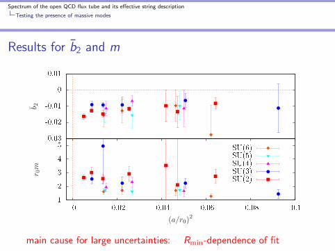
Results for b2 and m
-0.03
-0.02
-0.01
0
0.01
b 2
1
2
3
4
5
0 0.02 0.04 0.06 0.08 0.1
r 0m
(a/r0)2
SU(6)
SU(5)
SU(4)
SU(3)
SU(2)
main cause for large uncertainties: Rmin-dependence of fit
Spectrum of the open QCD flux tube and its effective string description
Testing the presence of massive modes
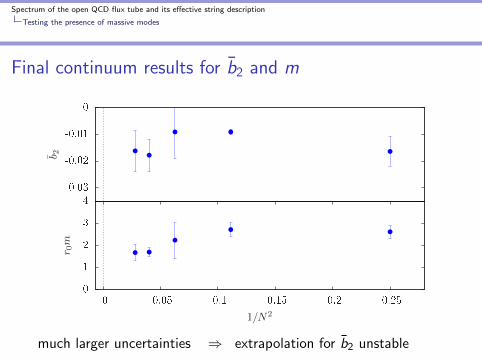
Final continuum results for b2 and m
-0.03
-0.02
-0.01
0
b 2
0
1
2
3
4
0 0.05 0.1 0.15 0.2 0.25
r 0m
1/N2
much larger uncertainties ⇒ extrapolation for b2 unstable
Spectrum of the open QCD flux tube and its effective string description
Testing the presence of massive modes
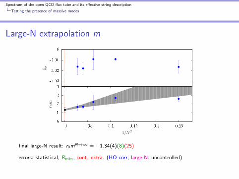
Large-N extrapolation m
-0.03
-0.02
-0.01
0
b 2
0
1
2
3
4
0 0.05 0.1 0.15 0.2 0.25
r 0m
1/N2
final large-N result: r0mN→∞ = −1.34(4)(8)(25)
⇒mN→∞√σ≈ 1.1
errors: statistical, Rmin, cont. extra. (HO corr, large-N: uncontrolled)
“worldsheet axion” (4d):mN→∞√σ≈ 1.713(4) [ Athenodorou, Teper, PLB771 (2017) ]

Spectrum of the open QCD flux tube and its effective string description
Testing the presence of massive modes
Large-N extrapolation m
-0.03
-0.02
-0.01
0
b 2
0
1
2
3
4
0 0.05 0.1 0.15 0.2 0.25
r 0m
1/N2
final large-N result: r0mN→∞ = −1.34(4)(8)(25) ⇒mN→∞√σ≈ 1.1
errors: statistical, Rmin, cont. extra. (HO corr, large-N: uncontrolled)
“worldsheet axion” (4d):mN→∞√σ≈ 1.713(4) [ Athenodorou, Teper, PLB771 (2017) ]
Spectrum of the open QCD flux tube and its effective string description
Testing the presence of massive modes
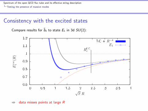
Consistency with the excited states
Compare results for b2 to state E1 in 3d SU(2):
0.6
0.7
0.8
0.9
1
1.1
1.2
0 0.5 1 1.5 2 2.5 3 3.5 4
Ersc
1(R
)
√σ R
RLCc
LC + R−4
E1
⇒ data misses points at large R
Spectrum of the open QCD flux tube and its effective string description
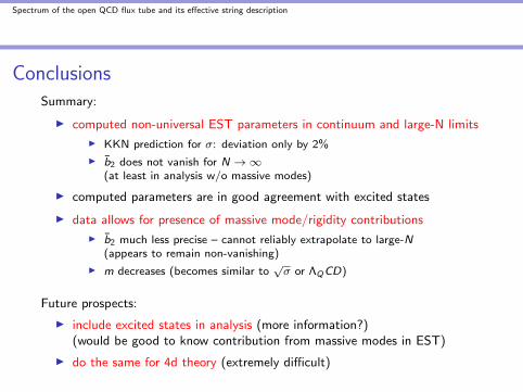
ConclusionsSummary:
I computed non-universal EST parameters in continuum and large-N limits
I KKN prediction for σ: deviation only by 2%
I b2 does not vanish for N →∞(at least in analysis w/o massive modes)
I computed parameters are in good agreement with excited states
I data allows for presence of massive mode/rigidity contributions
I b2 much less precise – cannot reliably extrapolate to large-N(appears to remain non-vanishing)
I m decreases (becomes similar to√σ or ΛQCD)
Future prospects:
I include excited states in analysis (more information?)(would be good to know contribution from massive modes in EST)
I do the same for 4d theory (extremely difficult)

Spectrum of the open QCD flux tube and its effective string description
Thank you for your attention!