arX

iv:1

309.

2572

v2 [

gr-q

c] 3

0 O

ct 2

013

The coordinate-independent Noether approach to energy-momentum localization

Ermis Mitsou∗

Departement de Physique Theorique and Center for Astroparticle Physics,

Universite de Geneve, CH–1211 Geneva, Switzerland

In this paper we are interested in the Noether currents associated to active diffeomorphisms, thatis, the pushforwards along the integral lines of any vector field. We work with exterior calculus overthe space-time manifold in the vielbein formalism of General Relativity, both with its first-order(Palatini) and second-order (Møller) formulations. We first derive some general properties of thesecurrents. The main novel result is that, if one decomposes all forms in the vielbein basis, then thevielbein acquires the same relation with the group of diffeomorphisms as does any gauge field withits corresponding gauge group. This also provides us with an alternative way for computing theNoether energy-momentum tensor, which is the subject of the second part of the paper.

The standard use of the Noether currents is to evaluate them on a holonomic basis of vectorfields, in which case one obtains an energy-momentum pseudo-tensor. In this paper we emphasize analternative set of privileged vectors, which is the Lorentz frame. The corresponding Noether currentsresult in an energy-momentum tensor under diffeomorphisms, but with a non-trivial dependence onthe frame. The corresponding energy charge is fundamentally different than in all the pseudo-tensorapproaches in that it does not correspond to a Hamiltonian boundary term. We provide a positivityproof for this energy definition that makes no use of coordinates and evaluate it on some standardspace-times for some distinguished frames.

I. INTRODUCTION & SUMMARY

The research on the localization of the energy and mo-mentum of the gravitational field has a long history goingback to the early years of General Relativity (GR) (seefor example the reviews in [1–3] and references therein).In this paper we study what Noether’s theorem, in itscoordinate-independent form, can tell us about this is-sue. We work in the vielbein formalism of GR and con-sider both the first and second-order formulations thatare the Palatini and Møller actions, respectively. In thevielbein context, the prevailing definition for the energy-momentum complex (pseudo-tensor1) is the one of Møller[4]. When on-shell, it is given as the divergence of asuperpotential M ν

µ = ∂ρUνρ

µ , where Greek letters de-note holonomic tensor indices, i.e. they correspond to acoordinate-induced basis of the tensor bundle. The su-perpotential obeys U νρ

µ = −U ρνµ , so that the complex

is conserved ∂νMν

µ = 0. Most importantly however, Uis a tensor density, i.e. it transforms homogeneously un-der coordinate transformations. This is something thatcan be only achieved using vielbeins, and thus the Møllercomplex is distinguished from all the pseudo-tensor ap-proaches of the metric formalism. The price to pay how-ever is that U νρ

µ is not invariant under local Lorentztransformations (LLTs), the internal gauge symmetry ofvielbein GR2. Nevertheless, the tensorial nature is a greatconceptual advantage and a frame dependence should be

∗ ermis.mitsou@unige.ch1 In this paper we use the word “tensor” for “tensor under diffeo-morphisms”.

2 Just as the coordinate dependence is unavoidable in the metricformalism, so is the frame dependence when using vielbeins. Inthis paper we use “frame” for “orthonormal frame” or “Lorentzframe”.

preferred over a coordinate one. Indeed, an (orthonor-mal) frame is the same data as the ones of the velocityfield and space-frame of a physical observer, while co-ordinates have really no physical interpretation. Froma field-theoretical point of view this might sound quiteheretic, because then the LLTs become the symmetrythat relates physical observers, i.e. they carry a physi-cal interpretation while at the same time being a gaugesymmetry. However, the frame – observer identificationtechnically makes sense and the LLT invariance of theaction can be interpreted as the fact that no observeris privileged, i.e. the relativity of observers. We thenfind it much more natural that the energy and momen-tum depend non-trivially on the observer than on thelabels we choose to attribute to the space-time points.In this paper, we therefore privilege as much as possiblecoordinate-independence and understand “observer” and“frame” as synonyms.Whether one uses pseudo-tensors, or tensors that

are non-covariant under LLTs, to describe the energy-momentum densities of gravity, one can always set theseto zero at a point using the appropriate coordinate or lo-cal Lorentz transformation, respectively. Therefore, onecan only attribute energy and momentum to submani-folds of dimension greater than zero [1]. Since here we ex-press these as Noether currents, it is natural to attributethem to space-like hypersurfaces Σ of codimension one.Therefore, only the energy-momentum charges may carryphysical information. In the case of the Møller complexfor instance, using a coordinate system such that t is thetime coordinate and Σ is of the form t = const, we wouldget (no µ summation)

PMølµ ≡ ηµµ

∫

Σ

M tµ dV = ηµµ

∫

∂Σ

U tνµ nνdS , (1)

where nµ is the normal to the boundary ∂Σ. This cor-

2

responds to the so-called “quasi-local” approach, wherethe result only depends on the fields at the boundary ofthat region. Now note that, although the local energy-momentum information of the Møller definition seemsto be contained inside of a tensor U , the way it entersthe definition of the corresponding charges breaks thatcovariance. Indeed, the above energy-momentum chargehas a bare µ-index so it is not covariant under generic co-ordinate transformations on ∂Σ, on top of its non-trivialframe dependence. In particular, the energy −PM

t is in-variant only under spatial diffeomorphisms that map ∂Σto itself. This may seem natural in the canonical con-text where one has already broken the diffeomorphismgroup by invoking a space-time foliation, but if one looksat it from the Lagrangian point of view, it is quite inele-gant. Therefore, this definition makes more compromisesthan necessary, because the frame dependence may beunavoidable, but the coordinate one is not.In this paper we study the option of minimum compro-

mise and thus define an energy-momentum tensor (EMT)for gravity. Its only non-trivial dependence will be onthe frame, and the corresponding charges will be invari-ant under any coordinate transformation3. The recipethat allows us to achieve this is principally made of twoingredients.The first one is the mathematical formalism we are go-

ing to use. The issue of energy and momentum in GR be-ing plagued by coordinate-dependent considerations, theappropriate framework for working this out is the oneof exterior calculus over the space-time manifold M. Itis an explicitly coordinate-independent and global way ofdisplaying and manipulating the field information. Apartfrom elegance, sticking to this formalism guarantees thatgeneral covariance is always preserved and prevents usfrom being distracted by coordinate-induced artefacts.Moreover, using some simple identities listed in appendixC, we will show that many computations in GR that areusually lengthy when carried out using coordinates be-come quite straightforward when using forms. We willthus work directly with the formal expression of fields,i.e. as global sections of the exterior bundle ofM, insteadof their local coordinate-induced representations that arefunctions from R4 to some set of numbers. For instance,we will consider the diffeomorphism group Diff(M) in thesense of homeomorphisms from M to M that are diffeo-morphisms in any local coordinate system. The actualdiffeomorphism group Diff

(

R4)

which is used in coordi-nate transformations does not appear in this explicitlycoordinate-independent formalism.The second ingredient is Noether’s theorem in the gen-

erally covariant context and in the language of differential

3 This tensor has already been considered in the literature (see forexample [1, 6, 8, 9]), but the charges are always defined with bareholonomic indices. Moreover, to our knowledge, it has never beenevaluated on concrete examples. The pseudo-tensor approachesare largely preferred for this in the literature.

forms. A conserved current is described by a closed d-form J , where D ≡ d + 1 is the manifold dimension. Itcan therefore be locally given by a superpotential (d−1)-form J ≡ dU . The notion of conserved charge is stillwell-defined although it must be understood in a broadersense. This is because there is no preferred space-likehypersurface to integrate the currents over, nor a pre-ferred “time direction” with respect to which the chargewould evolve. As a consequence, the conservation law ap-plies to any d-dimensional hypersurface Σ and any vectorfield ξ providing locally an evolution direction. More pre-cisely, the variation of the charge when the hypersurfaceis moved along the flow-lines of ξ is equal to the currentnormal to ξ integrated over ∂Σ. Because of this flexibil-ity, the theorem makes no distinction between global andlocal symmetries4.The beginning of the paper will be devoted to deriv-

ing Noether’s theorem in its covariant formulation and,subsequently, the Noether currents associated with activediffeomorphisms. Active diffeomorphisms are the repre-sentation of Diff(M) where the group acts on fields. Theycan be seen as the localization of the translational sym-metry, i.e. they correspond to the pushforwards alongthe integral lines of any vector field ξ. It turns out thatthe corresponding Noether current d-forms P [ξ] are non-trivially related to the Noether currents of the internalsymmetries of the theory, such as the LLT symmetryin Palatini gravity. This relation affects in a very pre-cise way the behaviour of P [ξ] under the internal gaugetransformations. Therefore, to get a good grasp on theNoether current of diffeomorphisms, we propose to con-sider, on top of the gravitational sector, a Yang-Mills(YM) field as well as a Dirac spinor, the prototypicalcouple of gauge theory. Moreover, we will see that thereare some very nice analogies one can draw between theNoether currents of internal symmetries and the one ofdiffeomorphisms. For instance, if one decomposes allforms in the vielbein basis, the transformation of thevielbein under diffeomorphisms and its relation to theassociated Noether current are formally analogous to thecase of a YM field, which leads to interpret the vielbeinas the gauge field of diffeomorphisms. The analogy ishowever limited because, while in the cases of internalgauge symmetries the Noether currents are covariant un-der any symmetry, P [ξ] is not covariant under internalgauge transformations.The matter part of the current can be easily improved

to a fully covariant tensor. The latter then coincides withthe definition of that object in GR, i.e. the variation ofthe matter action with respect to the vielbein. The grav-itational part, on the other hand, cannot be improvedto a fully covariant and yet non-trivial tensor. Thus, itinevitably maintains a dependence on the Lorentz frame.There is however another criterion with respect to which

4 Moreover, note that the family of hypersurfaces that the ξ-fluxgenerates this way does not have to be a foliation.

3

this tensor should be improved. It should be made onlyout of the first derivatives of the gravitational field, sinceits equation of motion is second-order in the derivatives.This is already the case for the Noether current corre-sponding to the Møller Lagrangian but not for the one ofPalatini theory. For the latter, we show how to improveit so that it meets the requirement and then both tensorsare the same when torsion vanishes.So for every vector field ξ we have an improved Noether

current T [ξ] that is conserved when on-shell and with theabove mentioned properties. To define an EMT, we needto evaluate T [ξ] on a basis of vector fields5. We distin-guish two privileged cases, the holonomic bases and theorthonormal bases. The former is induced by a local co-ordinate system ∂µ and, as is well known, the correspond-ing Tµ ≡ T [∂µ] is the expression of Møller’s complex inexterior calculus. Like any other pseudo-tensor complex,it can be understood as a Hamiltonian boundary term inthe canonical formalism [5]. The second choice amountsto taking the frame vectors ǫI themselves TI ≡ T [ǫI ],where the capital Latin letters denote Lorentz indices.The TI are tensors, since no coordinate system has everbeen invoked, and are therefore the minimal compromiseEMT that we consider in this paper. The correspondingcharges are Lorentz-indexed

T I ≡∫

Σ

T I =

∫

∂Σ

UI , (2)

and the superpotential 2-forms UI are known as the“Nester-Witten form” in the literature [8, 9]6. Whenexpressed in the language of contravariant superpoten-tial densities, the relation between the one of TI and theMøller complex Tµ is simply

U νρI = eµIU

νρµ . (3)

The corresponding complex is then a tensor density be-cause of the following identity involving the Levi-Civitaconnection

T νI ≡ ∂ρU

νρI = ∇ρU

νρI 6= eµIM

νµ , (4)

holding precisely because of the νρ antisymmetry and thefact that U νρ

I is a tensor density of weight one. As we

5 Actually, active diffeomorphisms are actually a generalization ofthe whole (active) Poincare group, since rotations and boostsare also generated by vector fields. For example, a space-likevector field whose integral lines have R-topology (or S1 but thatare not contractible to a point in M) would be interpreted asgenerating a space translation, while if the lines have S1-topologythat can be contracted to a point in M, then the vector fieldwould be generating a rotation. Therefore, we get an EMT,in the traditional sense, only if the basis on which we evaluateT [ξ] is Cartesian-like, whereas if it is polar-like we rather get an“energy-angular/radial-momentum tensor”.

6 More precisely, the Nester-Witten form is actually defined as aform on the frame bundle F (M) and the form we have here isits pullback along a section of F (M) which is an orthonormalframe.

will see, related to the fact that T νI is a tensor is the

fact that its associated energy charge is not a Hamilto-nian boundary term. Another interesting property of TI ,which is analogous to the EMT of a YM field, is the factthat it is traceless in four dimensions. We also show thatfor every space-like hypersurface Σ there exists observersfor which the total energy in Σ is positive.Finally, we evaluate the total energy charges on some

standard space-times in some physically distinguishedframes. For a Schwarzschild black hole a stationary ob-server measures a total energy of M , the mass of theblack hole, while a radially free-falling observer measuresno energy at all. For a stationary observer on de-Sitterspace-time, we get a total energy of 8πH−1 inside thehorizon, whereH is the Hubble parameter, a result whichis discontinuous in the H → 0 limit. For a comoving ob-server in FLRW space-time, we find a zero energy densityunless we have spatial curvature, in which case the signis the one of the curvature parameter k. We will see thatthe energy density can be sometimes negative, even forasymptotically trivial space-times and observers.The organization of the paper goes as follows. In sec-

tion II we introduce our notational conventions. In sec-tion III we derive the tools of interest that are the varia-tional principle and Noether’s theorem. In section IV wediscuss the issue of the EMT and corresponding chargesin generally covariant field theory. In section V we com-pute the energy of some standard GR solutions. In sec-tion VI we draw our conclusions.

II. SETUP, CONVENTIONS AND NOTATION

A. Geometry and groups

Let M be a real parallelizable smooth manifold ofdimension D ≥ 4 and let ∆k denote the set of k-dimensional orientable closed embedded submanifolds ofM. For U ∈ ∆D, X(U) ≡ Γ(TU) denotes the space ofvector fields and Ωp(U) ≡ Γ (Λp(U)) denotes the spaceof p-forms, over U . If the U dependence is omitted thenit means the assertion works for all U ∈ ∆D.The parallelizability of M implies the existence of

global non-singular vielbein7 1-forms eI , i.e. eI1 ∧ . . . ∧eID 6= 0 everywhere on M. This implies that eI is abasis of Ω1(M) and therefore that there exists a uniqueglobal basis of ǫI ∈ X(M), defined by eI(ǫJ) = δIJ , be-ing the frame, or inverse vielbein. In any local coor-dinate system, we denote the components of eI and ǫIin the corresponding holonomic bases by eIµ and eµI , re-

spectively, and also e ≡ det(

eIµ)

. Whenever we invokecoordinates xµ, we let t denote the time-like one, i.e.gtt ≡ g (∂t, ∂t) < 0 and xa the space-like ones, gaa > 0,

7 In the literature “vielbein” is used for the frame vectors but herewe choose it to refer to the co-frame.

4

where a = 1, . . . , d. The Lorentzian metric field is definedby g ≡ ηIJ e

I ⊗ eJ , where ηIJ is the Minkowski metricand we choose it with a signature of mostly pluses. Wedefine the compact notations eI1...Ip ≡ eI1 ∧ . . . ∧ eIp ,eI1...Ip ≡ εI1...IDe

Ip+1...ID/(D − p)!, iI1...Ip ≡ iI1 . . . iIpand LI ≡ LǫI , where for the Levi-Civita symbol we usethe convention ε012...D = −ε012...D = 1, iI denotes theinterior product and LI the Lie derivative with respectto ǫI . Replace I → ξ for an arbitrary vector field ξ. TheHodge dual is defined by

⋆ α ≡ 1

p!eI1...IpiIp...I1α , α ∈ Ωp . (5)

We use d to denote the exterior derivative, D to denotethe covariant exterior derivative with respect to all in-ternal gauge transformations and ∇ for the Levi-Civitaconnection, i.e. the covariant derivative with respect todiffeomorphisms (only) employing the Christoffel sym-bols Γ[g]. We let d denote the codifferential

dα ≡ (−1)D(p−1) ⋆ d ⋆ α , α ∈ Ωp . (6)

We adopt the mathematicians convention for the Lie al-gebra of a Lie group, i.e. the latter is the exponentiationof the former with no i factor. For the case of SU(N) forexample, we have that the fundamental representationof su(N) is the set of traceless complex N ×N matricesobeying α + α† = 0. The basis of su(N) is chosen suchthat

[

T a, T b]

= fabcT c , Tr(

T aF , T

bF

)

= −1

2δab (7)

where the structure coefficients fabc are totally antisym-metric and the “F” subscript denotes the fundamentalrepresentation. The indices of T a

F will be given by greekletters of the end of the alphabet, i.e. the matrix elementsare (T a

F)στ .

For the LLTs, since we are not going to be interestedon the discrete part of the group, let us directly say that“LLT” holds for the local action of the component con-nected to the identity SO1(1, d). Since we are also goingto consider spinors, the actual group that acts on the Iindices is Spin(1, d), the double cover of SO1(1, d). Thestandard choice of basis of spin(1, d) is the one obeyingthe Lorentz algebra[

T IJ , TKL]

= ηILT JK − ηJLT IK − ηIKT JL + ηJKT IL ,(8)

where the generators T IJ are antisymmetric in the IJindices. The vector and Dirac representations read

(

T IJv

)K

L= ηIKδJL − ηIKδJL , T IJ

D =1

2γIJ , (9)

respectively, where γI1...Ip ≡ γ[I1 . . . γIp] and the γI obeythe Clifford algebra γI , γJ = 2 ηIJ . There are two(anti)commutation relations that will be useful for us[

γI , γJK]

= ηIJγK − ηIKγJ , γI , γJK = 2 γIJK .(10)

We choose a representation of complex dimension 2[D/2]

and where(

γI)†

= ηIIγI (no summation implied).Defining the bar conjugation so that it is an involution

ψ ≡ ψ†iγ0, we get γI ≡ iγ0(

γI)†iγ0 = −γI and thus

γI1...Ip = (−1)pγIp...I1 = (−1)p(p+1)/2γI1...Ip . (11)

In particular, γIJ = −γIJ so that the Dirac representa-tion of spin(1, d) is the set of matrices obeying θ+ θ = 0.We will use greek indices from the beginning of the al-

phabet for the elements of these matrices, i.e.(

γIJ)αβ

.Let Diff(M) denote the group of diffeomorphisms of

M and let Diff1 (M) denote its component connectedto the identity. Every vector field ξ ∈ X(M) generatesa one-parameter family of diffeomorphisms Ξtt∈I⊂R ⊂Diff1(M) with I ∋ 0 defined by

Ξ0 = id , Ξt

∣

∣

∣

t=0= ξ . (12)

Inversely, by definition of Diff1(M), every element Ξ ∈Diff1(M) sufficiently close to the identity can be thoughof as the t = 1 element of the family generated by someξ. In analogy with the theory of Lie groups of finite di-mension, we can thus say that X(M) is the “Lie algebra”of Diff1(M). This is the fundamental representation ofDiff1(M), also known as “passive diffeomorphisms”, butthe ones of interest here are the tensor representations,also known as “active diffeomorphisms”. In that case theΞ ∈ Diff1(M) acts on a section T of a bundle based onM through the pushforward map

T ′ = Ξ∗T . (13)

By definition, the infinitesimal variation then involves theLie derivative in the corresponding ξ direction8

δT = −LξT ⇒ Ξ∗ = e−Lξ . (14)

Thus, the generators in that representation are the Liederivatives and, given the properties of L, obey the fol-lowing algebra

[Lξ,Lξ′ ] = L[ξ,ξ′] , (15)

where [ξ, ξ′] is the Lie bracket, the algebraic product ofX(M). There are two privileged types of bases for theLie algebra X(M). One is given by the vector fields ∂µinduced by some local coordinate system, in which casethe Lie bracket is trivial but the normalization is not

[∂µ, ∂ν ] = 0 , g (∂µ, ∂ν) = gµν . (16)

8 Actually, the Lie derivative is defined as the generator of pull-backs, but since Ξ is a bijection, the infinitesimal pushforwardwith respect to Ξξ is well-defined and equal to the infinitesimalpullback with respect to Ξ

−ξ, hence the minus sign.

5

The other choice are the frame vectors ǫI , where thingsare the other way around

[ǫI , ǫJ ] = C KIJ ǫK , g (ǫI , ǫJ) = ηIJ . (17)

The CIJK are known as the “structure coefficients” and,in terms of the vielbein, they are given by CIJK ≡iIJdeK .

B. Fields and Lagrangians

We use totally dimensionless units ~ = c = 8πG = 1.The fields of the theory we are going to consider arethe veilbein eI ∈ Ω1(M) in the fundamental represen-tation of Spin(1, d), the spin connection ωIJ ∈ Ω1(M)in the adjoint representation of Spin(1, d), the YM fieldAa ∈ Ω1(M) in the adjoint representation of SU(N), andthe Dirac spinor in the Dirac/fundamental representa-tion of Spin(1, d)⊗SU(N) ψασ ∈ Ω0(M)⊗G, where G isthe set of complex Grassmann numbers. The non-trivialinfinitesimal variations under an SU(N) transformationwith parameter α = αaT a ∈ Ω0(M)⊗ su(N) are

δAa = −Dαa ≡ −dαa + fabcαbAc , δψ = αaT a ψ ,(18)

where it is understood that for the spinor T a ≡ T aF . Un-

der an LLT with parameter θ = 12 θIJT

IJ ∈ Ω0(M) ⊗spin(1, d) we have

δeI = θIJeJ ,

δωIJ = −DθIJ ≡ −dθIJ + θ KI ωKJ − θ K

J ωKI ,

δψ =1

4θIJ γ

IJ ψ , (19)

and under a diffeomorphism with parameter ξ ∈ X allfields transform as (14). The LagrangianD-form is givenby

L ≡ Lg + Lm , (20)

where Lg is the gravitational part and Lm the matterpart of the Lagrangian. For gravity we are going to con-sider two Lagrangians. The first-order one is the PalatiniLagrangian

LP ≡ 1

2ΩIJ ∧ eIJ , (21)

where ΩIJ ≡ dωIJ + ω KI ∧ ωKJ are the curvature two-

forms of the spin connection. The second-order one isthe Møller Lagrangian

LM ≡ −1

2

(

F IJ ∧ ⋆ F J

I −1

2F ∧ ⋆ F

)

, (22)

where F IJ ≡ eI ∧ deJ and F ≡ F II . It is related to

the Einstein-Hilbert Lagrangian by a total derivative, asshown in appendix A. It will be more convenient for com-puting directly the EMT of gravity, but we will prefer

treating with the Palatini Lagrangian since it is moretransparent and its structure is closer to YM theory. Inthe matter sector we have the YM Lagrangian

LYM ≡ − 1

2g2F a ∧ ⋆ F a , (23)

where

F a = dAa +1

2fabcAb ∧ Ac , (24)

are the curvature two-forms of Aa. Finally, we also con-sider a massless Dirac field whose Lagrangian reads

LD ≡ Re[

ψγIDψ]

∧ eI =1

2

[

ψγIDψ −DψγIψ]

∧ eI

=1

2

[

ψγIdψ − dψγIψ]

∧ eI

+1

4ωIJ ∧ eK ψγIJKψ +Aa ∧ eI ψT aγIψ . (25)

where we have used the exterior covariant derivative inthe appropriate representations

Dψ ≡(

d +1

4ωIJ γ

IJ +AaT a

)

ψ ,

Dψ ≡ Dψ = dψ − 1

4ωIJ ψγ

IJ −AaψT a , (26)

the definition of complex conjugation on complex Grass-mann numbers

(

ψασψβτ)∗

= ψβτ∗ψασ∗, and (10). Un-less mentioned otherwise, we will be using the followingtheory for illustrating our arguments

L = LP + LYM + LD . (27)

III. LAGRANGE - NOETHER FORMALISM

The first section concerns the equations of motion ofthe theory and it will provide us with some useful for-mulas for dealing with Noether currents. It can also beseen as a warm-up for using the technology of exteriorcalculus.

A. The variational principle

Let φa ∈ Ωp(M) ⊗ K, with a = 1, . . . , N and K = R,C or G, be a set of N p-form fields. They are given witha Lagrangian L = L (φ, dφ) ∈ ΩD(M) which is local, i.e.the values of L at p ∈ M only depend on the values of φa

and dφa at that same point. We will also ask that L bepolynomial in dφa. To our Lagrangian there correspondsan action functional

S ≡∫

M

L , (28)

and the variational principle goes as follows. We start byconsidering a field configuration φa and an infinitesimal

6

variation φa → φa + δφa over M. The variation of dφa

being determined by the one of φa, i.e. δdφa = dδφa, thevariation of the Lagrangian is given by

δL = δφa ∧ ∂L

∂φa+ dδφa ∧ ∂L

∂dφa. (29)

The operators ∂∂φa and ∂

∂dφa are defined as anti-

derivations of degree −p and −(p+ 1), respectively, sat-isfying

∂

∂φaφb = δba ,

∂

∂dφadφb = δba , (30)

have the same Grassmann degree as φa and we conven-tionally apply them from the left. The above equationsand the fact that they are anti-derivations determinethem on all of Ω(M). Now the variation of the actionbeing

δS =

∫

M

δL =

∫

M

(

δφa ∧ ∂L

∂φa+ dδφa ∧ ∂L

∂dφa

)

,

(31)we integrate by parts the second term and find

δS =

∫

M

δφa∧(

∂L

∂φa− (−1)pd

∂L

∂dφa

)

+

∫

∂M

δφa∧ ∂L

∂dφa.

(32)To get rid of the boundary term we have to restrict tovariations such that δφa|∂M = 0, for the fields obeying∂L

∂dφa 6= 0. The classical solutions of the theory given by

L are the field configurations which make δS vanish forall such δφa and therefore obey

ELa ≡ ∂L

∂φa− (−1)pd

∂L

∂dφa= 0 . (33)

These are the Euler-Lagrange equations in exterior cal-culus. Finally, note that these equations imply that the(D − p)-form

Ja ≡ −(−1)p∂L

∂φa(34)

is exact when evaluated on a classical solution and thusdJa = 0. If p = 0, then this is a trivial identity sinceJa ∈ ΩD(M), but if p > 0, then this is a genuine conser-vation equation, valid on classical solutions. It is there-fore not surprising that it will have a direct relation withthe Noether currents in the case where p = 1, as we willsee later on. For later reference, we will call these d-formsJa the “Euler-Lagrange”, or simply, “EL” currents.

1. Example

The equation of motion of the vielbein is

ELI ≡ ∂L

∂eI+ d

∂L

∂deI= −GI + TI = 0 , (35)

where

GI ≡ −δSP

δeI= −∂LP

∂eI− d

∂LP

∂deI(C2)= −1

2eIJK ∧ ΩJK ,

(36)is the analogue of the Einstein tensor in first-order viel-bein GR and

TI ≡ δSm

δeI=∂Lm

∂eI+ d

∂Lm

∂deI

(C2)(C16)(C11)=

1

2g2(iIF

a ∧ ⋆ F a − F a ∧ iI ⋆ F a)

−Re[

ψγJDψ]

∧ eJI , (37)

is the analogue of the matter energy-momentum tensor asdefined in GR, i.e. as the variation of the matter actionwith respect to the vielbein. The equation of motion ofthe spin connection is

ELIJ ≡ ∂L

∂ωIJ+ d

∂L

∂dωIJ=

1

2DeIJ +

1

4ψγIJKψ e

K

(C3)=

1

2eIJK ∧ΘK +

1

4ψγIJKψ e

K = 0 , (38)

where ΘI ≡ deI + ωIJ are the torsion two-forms. Multi-

plying (38) by eL and using (C2) we get

eIJ ∧ΘL + 2 ηL[I eJ]K ∧ΘK = −1

2ψγIJLψ e (39)

Then, taking the Hodge dual and using (C15) we obtain

ΘIJL + 2 ηL[IΘJ]K

K =1

2ψγIJLψ , (40)

where ΘIJK ≡ iIJΘK . Taking the JL trace impliesΘIJ

J = 0 so these are equivalent to

ΘIJK =1

2ψγIJKψ , ⇔ ΘI = −1

4ψγIJKψ eJK .

(41)One can thus always explicitly solve for ωIJ

ωIJ = ωIJ [e] +1

4ψγIJKψ e

K , (42)

where ωIJ is the Levi-Civita spin connection defined im-plicitly as the unique torsion-free spin connection deI =−ωI

J ∧ eJ , and totally determined by the vielbein9.Thus, LP is classically equivalent to LEH only if thereare no spinors, or if we always couple them to the Levi-Civita spin connection. In the theory we consider on theother hand, integrating out ωIJ produces a non-linearspinor sector, and more precisely a spin-spin interaction

∼(

ψγIJKψ)2e. Therefore, classically, the difference be-

tween the two gravitational theories can be translated

9 An alternative definition is

∇ǫI ǫJ = −ω KIJ ǫK , ωIJK ≡ iI ωJK . (43)

7

into a difference in the spinor Lagrangian. The equationof motion of Aa gives

ELa ≡ ∂L

∂Aa+ d

∂L

∂dAa

(C11)= − 1

g2

[

∂F b

∂Aa∧ ⋆ F b + d

(

∂F b

∂dAa∧ ⋆ F b

)]

+eI ψTaγIψ

= − 1

g2[

d ⋆ F a + fabcAb ∧ ⋆ F c]

eI ψTaγIψ

≡ − 1

g2D ⋆ F a + eI ψT

aγIψ = 0 . (44)

Finally, the equation of motion of ψασ is

ELασ ≡ ∂L

∂ψασ− d

∂L

∂dψασ(45)

(C3)(C8)=

[

γIdψ +1

2ωI

JγJψ

+1

4ωJK γIJKψ +AaT aψ

]ασ

∧ eI

=

[

γIDψ +1

4KJKγ

IJKψ

]ασ

∧ eI = 0 ,

where we have used (10), D is the covariant derivativeusing the Levi-Civita connection and KIJ ≡ ωIJ − ωIJ

is the contorsion tensor. The equations of motion of theψασ are then minus the complex conjugate. We have thusretrieved the Palatini, Yang-Mills and Dirac equations ofmotion from a variational principle without ever havingto introduce coordinates. Finally, we have three non-zeroform fields and the corresponding EL currents are

JI ≡ ∂L

∂eI= ELI , (46)

JIJ ≡ ∂L

∂ωIJ= −ω[I

K ∧ eJ]K +1

4ψγIJKψ eK , (47)

Ja ≡ ∂L

∂Aa= − 1

g2fabcAb ∧ ⋆ F c + eI ψT

aγIψ . (48)

Note that the one of eI is zero on-shell since the La-grangian does not depend on deI .

B. Noether’s theorem

1. Currents

A continuous symmetry is an active transformation10

of the fields under a continuous group whose infinitesimalversion makes the Lagrangian transform as

δL = −dK , (49)

10 As already explained for the case of diffeomorphisms, here by“active transformation” we mean a map sending a section, infibre bundle language, to another section.

for some d-form K. Equivalently, the transformation isa symmetry if the action is invariant up to a bound-ary term. Noether’s theorem states that to every suchsymmetry there corresponds a d-form J , the Noethercurrent, which is conserved when evaluated on classicalsolutions, i.e. we have an identity dJ ∼ EL. In quantumfield theory one is rather accustomed to working with thedual current 1-form j ∈ Ω1(M), defined as J ≡ ⋆ j, forwhich the above equation is expressed in terms of the cod-ifferential dj ∼ EL. In any coordinate system this takesthe usual form of the current divergence dj ≡ ∇µj

µ.Given that for a vector field jµ ≡ gµνjν

∇µjµ = e−1∂µ (ej

µ) , (50)

where e ≡ det(eIµ) is the volume density, it is cus-tomary to rather use the vector density ejµ to repre-sent the current, so that the conservation equation reads∂µ(ej

µ) = 0. It is however the d-form J which is thenatural coordinate-independent representation of a “cur-rent”, since the latter must be integrated over a d-volumein order to give a charge, so it must be a d-form. Eventhe conservation equation is simpler in terms of J sinced is an anti-derivation while d is not.To determine J , and thus prove the theorem, we com-

pute the infinitesimal variation of the Lagrangian but asinduced by the one of the fields

δL = δφa ∧ ∂L

∂φa+ dδφa ∧ ∂L

∂dφa

(33)= δφa ∧ ELa + (−1)pδφa ∧ d

∂L

∂dφa+ dδφa ∧ ∂L

∂dφa

= δφa ∧ ELa + d

(

δφa ∧ ∂L

∂dφa

)

. (51)

Equating this with (49) and defining the d-form

J ≡ δφa ∧ ∂L

∂dφa+K , (52)

one gets the desired identity

dJ = −δφa ∧ ELa . (53)

Eq. (52) is therefore the definition of the Noether cur-rents.

2. Example

We consider again the theory (27) and the Noether cur-rents associated with the internal transformations. Wewill use a shorthand notation πa ≡ −g−2 ⋆F a to simplifyour expressions. The variations are given in (18) and(19) and the Lagrangian is invariant so K = 0. Thus, byNoether’s theorem, the currents associated to the trans-formations generated by α = αaT a ∈ Ω0(M) ⊗ su(N)and θ = 1

4 θIJγIJ ∈ Ω0(M)⊗ spin(1, d) are

J [α] ≡ δAa ∧ ∂L

∂dAa+ δψασ ∂L

∂dψασ+ δψασ ∂L

∂dψασ

=(

dαa + fabcAb αc)

∧ πa + αa eI ψTaγIψ , (54)

8

and

S[θ] = δeI ∧ ∂L

∂deI+ δωIJ ∧ ∂L

∂dωIJ(55)

+δψασ ∂L

∂dψασ+ δψασ ∂L

∂dψασ

= −1

2

(

dθIJ − 2 θ KI ωKJ

)

∧ eIJ +1

4θIJ eK ψγIJKψ ,

respectively. The fact that these currents are conservedon-shell for any α and θ is the mark of the redundancyin the apparent number of degrees of freedom in a gaugetheory. We then consider the special cases

J a ≡ J [T a] = fabcAb ∧ πc + eI ψTaγIψ = Ja , (56)

SIJ ≡ S[

T IJ]

= ω[IK ∧ eK|J] +

1

4eK ψγIJKψ = JIJ .

As anticipated earlier, the EL currents Ja ≡ ∂L∂Aa and

JIJ ≡ ∂L∂ωIJ

are thus nothing but a special subset ofthe Noether currents associated with the groups A andω gauge, respectively. Moreover, these currents are theones one obtains in the case where the gauge field is ab-sent and the symmetry is only global. Here we see thatby gauging the symmetry, we obtain a whole lot of newconserved currents that are indexed by geometric objectsthat are the fields α and θ in the adjoint representationof their respective groups.Now, all of these currents are not independent but can

be expressed in terms of Ja and JIJ using (54) and (56)

J [α] = αaJa−dαa∧πa , S[θ] = θIJJIJ − 1

2dθIJ ∧ eIJ

(57)Using the equations of motion Ja = −dπa and JIJ =− 1

2 deIJ , we get that on classical solutions

J [α]|EL=0 = −αadπa − dαa ∧ πa = −d (αaπa) , (58)

S[θ]|EL=0 = −1

2

(

θIJdeIJ + dθIJ ∧ eIJ

)

= −1

2d(

θIJ eIJ)

.

Thus, the Noether currents are not only closed formsbut also exact, i.e. the Poincare lemma holds globallyfor them. This is actually due to the fact that we assumethe solutions to the equations of motion to be global.It is important to understand the difference between

J [α] and J a. The former is the Noether current asso-ciated to a covariant field α and is thus gauge-invariant,as can be seen in (54). On the other hand, the EL cur-rent J a corresponds to the fixed choice α = T a and thustransforms inhomogeneously. Note finally that J [α] isR-linear in its argument

J [α+ β] = J [α] + J [β] , J [c α] = cJ [α] , (59)

for all c ∈ R. Of course, what has been said for J [α] inthis paragraph holds analogously for S[θ] as well.

3. Charges

Consider a Noether current J evaluated on a givenfield configuration φa which is not necessarily a classical

solution. We can construct the corresponding Noethercharge Q contained in a region Σ ∈ ∆d, that is, define amap

Q : ∆d → R

Σ 7→ Q (Σ) ≡∫

Σ

J . (60)

Let us now show the conservation law in terms of Q.We start by choosing a local evolution direction, thatis, a vector field ξ ∈ X(M). We then consider the one-parameter subgroup Ξtt∈I⊂R of Diff1(M) that it gen-erates, i.e. the one satisfying

Ξ0 = id , Ξt

∣

∣

∣

t=0= ξ . (61)

We also consider the continuous one-parameter familyof submanifolds Σt ≡ Ξt(U), the corresponding chargesQ(t) ≡ Q(Σt) and also define the “tube”

W ≡⋃

t∈I

Σt . (62)

Thus, Q(t) is the charge contained in the Σt hypersur-face and the latter evolves along the flow-lines of ξ. Thevariation of Q(t) with respect to t gives

Q(t) ≡ limǫ→0

1

ǫ[Q(Σt+ǫ)−Q(Σt)]

= limǫ→0

1

ǫ

[

∫

Ξt+ǫ(Σ)

J −∫

Ξt(Σ)

J]

=

∫

Σ

limǫ→0

1

ǫ

[

Ξ∗t+ǫJ − Ξ∗

tJ]

≡∫

Σ

Ξ∗tLξJ =

∫

Σt

LξJ

=

∫

Σt

(iξd + diξ)J =

∫

Σt

iξdJ +

∫

∂Σt

iξJ , (63)

where Ξ∗t is the pullback with respect to Ξt and we have

used the definition of the Lie derivative as the generatorof pullbacks. Focusing from now on on solutions of theequations of motion for φa, the first term drops by currentconservation and we are left with

Q(t)∣

∣

∣

EL=0=

∫

∂Σt

iξJ , (64)

which is the Noether conservation law in terms of thecharge: the variation of the charge within Σt is entirelydetermined by the current normal to ξ at the boundary.More precisely, the vector field ξ determines the shapeof the boundary of W and iξJ ∼ ⋆

(

ξ ∧ j)

. Therefore,this expression captures the part of j which is normal to∂W . The standard use of this law is the case where theΣt are space-like and ξ is time-like. It then reduces tothe fact that the variation of the charge in time insidethe space-region Σt is equal to the integrated currentflux through the boundary of W at the level t. Thistakes both into account the flow of the current out ofthe volume and the fact that the volume itself may vary

9

with time. Moreover, it also holds for arbitrary local timedirections ξ and space-like hypersurfaces Σ.As shown in the example given above, the on-shell

Noether currents are not only closed forms but also exact,so we can express the charge in terms of the superpoten-tial on the boundary

Q(Σ)|EL=0 =

∫

∂Σ

U . (65)

In this form, the fact that the variation of the charge isdetermined only by the fields on ∂Σ is trivial. Moreover,we see that in generally covariant field theory bound-aries are extremely important. Indeed, one cannot sim-ply consider the cases where all fields are trivial at spatialinfinity, as in special-relativistic field theory for instance,because this makes the total charges zero. The chargedoes not only vary by a boundary term under the ξ-flow,it is a boundary term itself.Consider now the argument that allows to construct

charges using the EL currents J a in special-relativisticfield theory. When on-shell, these currents vary by atotal derivative under a gauge-transformation, so the to-tal charges vary by a boundary term. Since the fieldsare trivial at spatial infinity, the total charges are gauge-invariant, i.e. well-defined physical observables. Giventhe above discussion, this argument no longer holds inGR since all the charge information lies on the boundaryanyway. Thus, one must now ask for gauge-invariant cur-rents in order to have well-defined observables. We haveseen that this is the case for the currents corresponding tointernal symmetries. Unfortunately, we will see that thiswill not be possible for the diffeomorphism symmetry,where the corresponding currents will have a non-trivialtransformation under LLTs. Thus, the energy and mo-mentum charges will depend on the choice of frame atthe boundary of U .

IV. THE NOETHER CURRENT OF

DIFFEOMORPHISMS

Let us now consider the Noether current associated todiffeomorphisms. All fields transform infinitesimally as

δφa = −Lξφa = −iξdφa − diξφ

a . (66)

General covariance of the theory implies that the La-grangian is a tensor, and more specifically a D-form, sodL = 0 and thus δL = −diξL, which is a total deriva-tive and therefore we have a symmetry. Following thederivation of Noether’s theorem, we have K = iξL andδφa = −Lξφ

a, so the Noether current associated to thediffeomorphism in the ξ direction is

P [ξ] = −Lξφa ∧ ∂L

∂dφa+ iξL . (67)

This is minus the generalized Hamiltonian in the lan-guage of [5, 7]. Just like in the case of internal symme-tries, we can compute the current corresponding to the

basis elements of the “Lie algebra” X(M). If we expectto relate this object to the EL current of the vielbein, byanalogy with the internal symmetries, we must give it anI index, so we choose the ǫI basis yielding the NoetherEMT

PI ≡ P [ǫI ] = −LIφa ∧ ∂L

∂dφa+ iIL . (68)

The problem with this expression is that, unlike in thecase of internal symmetries, the EL current of eI is nota Noether current PI 6= ∂L

∂eI . This can be easily seen bynoting that the only non-trivial step in computing thelatter is when ∂

∂eI acts on ⋆, whose solution is given by(C16). This cannot produce a term ∼ diIφ

a which ispresent in (68) through LIφ

a for matter forms of non-zero degree. Moreover, if we express P [ξ] in terms of thePI using (67)

P [ξ] = ξIPI − dξI ∧ iIφa ∧∂L

∂dφa, (69)

and compare with (57), we see that there are a priori alsomatter fields in the second term. Thus, we cannot yetdeduce the superpotential corresponding to P [ξ]. Thisissue is addressed in the following section.

A. The gauge field of diffeomorphisms

The problem raised above is related to the fact that,because of the existence of a vielbein, an ambiguity arisesregarding precisely non-zero forms. Should one take thep-forms φa as the independent fields, or should one ratherconsider their components in the vielbein basis φaI1...Ip ≡iIp...I1φ

a ∈ Ω0? We will call the first case the “standardpoint of view” while the second one will be the “scalars+ vielbein point of view”, since in that case all fieldsbut the vielbein are scalars under Diff(M). Using φa todenote all fields but the vielbein from now on, we havethe two theories

Lstd ≡ Lstd[

φa, eI]

, Ls+v ≡ Ls+v[

φaI1...Ip , eI]

.

(70)The standard point of view is well suited to gauge theorysince the EL currents and holonomies make use of thegauge field 1-forms, not the scalars. Moreover, the gaugetransformations of the gauge fields in terms of the scalarsmake use of the inverse vielbein, so they are less natural.As we will show now, the scalars + vielbein point ofview, however, is well suited for gravity because then thevielbein formally behaves as the gauge field associated todiffeomorphisms, i.e. in total analogy with the propertiesof the gauge fields we have seen until now.The first thing to show of course, is that both points of

view are classically equivalent, i.e. that their equationsof motion imply one another. This is a priori obvioussince the two choices of independent fields are related by

10

a non-linear but bijective field redefinition,

φa =1

p!φaI1...Ip e

I1...Ip , φaI1...Ip = iIp...I1φa . (71)

We choose to show this explicitly in appendix B because,in the process, we see that one can choose a mixed pointof view for the equations of motion, i.e. compute them inthe scalars + vielbein one for the vielbein and in the stan-dard one for the rest of the fields. We also show that theNoether currents are the same, even though some fieldshave changed Spin(1, d) and Diff1(M) representations.So let us consider the Ls+v theory, and for notationalsimplicity let us absorb the I indices in the generic in-dex a, i.e. let us write φa ≡ φaI1...Ip and keep in mind

that now φa ∈ Ω0(M). The key property of the scalars+ vielbein point of view is that the Lie derivative withrespect to ǫI becomes simply

LI |s+v = iId , (72)

on all fundamental fields, since iIφa = 0 and iIe

J = δJI .Considering the ǫI basis for X(M) means that we takeLI = iId as our generators in the active representation ofDiff1(M). These are nothing but the ǫI vectors seen asderivations. Then, under an infinitesimal diffeomorphismthe 0-forms transform homogeneously

δξφa = −Lξφ

a = −ξILIφa , (73)

while the vielbein is the only field transforming inhomo-geneously

δξeI = −Lξe

I = −dξI − ξJLJeI . (74)

Note the analogy with the transformation of Aa in (18)and ωIJ in (19). We have the same inhomogenous part,while the homogeneous one is the Lie derivative in dif-ferent respective senses. Here it is the Lie derivativewith respect to the base manifold M, while for the inter-nal transformations it is the Lie derivative with respectto the SU(N) and Spin(1, d) fibres11. Thus, the viel-bein formally transforms as the gauge field associated toDiff1(M). The Noether energy-momentum tensor (68)now reads

PI = −iIdeJ ∧ ∂Ls+v

∂deJ− iIdφ

a ∧ ∂Ls+v

∂dφa+ iIL

s+v , (76)

11 Indeed, in those cases one can write the transformations in termsof the algebra-valued fields A ≡ AaTa ∈ Ω1(M) ⊗ su(N) andω ≡ 1

2ωIJT

IJ ∈ Ω1(M)⊗ spin(1, d) where it reads

δA = −Dα = −dα− [A,α] , δω = −Dθ = −dθ − [ω, θ] ,(75)

and the commutator with α, θ is nothing but the Lie derivativein the α, θ directions, seen as left-invariant vector fields, on theirrespective group manifolds.

and the general Noether current associated to the diffeo-morphism in the ξ direction (69) is

P [ξ] = ξIPI − dξI ∧ ∂Ls+v

∂deI. (77)

This result is again analogous to the case of the internalsymmetries, see (57).

The antiderivations iI and ∂∂eI now have a lot in com-

mon. Since they are equal on vielbein products, andnow all fields have been decomposed into linear combi-nations of vielbein products, they are also equal whenacting on any combination of the fields which does notcontain derivatives, like the potential part of Ls+v for in-stance. For forms containing derivatives however they dodiffer since

∂

∂eIdφa = 0 6= iIdφ

a . (78)

Thus, acting with iI on Ls+v we get ∂Ls+v

∂eI plus terms

∼ iIdeJ and ∼ iIdφ

a. Since Ls+v is polynomial in deI

and dφa, the extra term which is not captured by ∂∂eI

issimply

iILs+v− ∂Ls+v

∂eI= iIde

J∧ ∂Ls+v

∂deJ+iIdφ

a∧ ∂Ls+v

∂dφa. (79)

Now, isolating ∂Ls+v

∂eIand using (76), we get

PI =∂Ls+v

∂eI, (80)

which is again analogous to the case of internal symme-

tries: the EL current of the vielbein J s+vI ≡ ∂Ls+v

∂eI isnothing but a special case of the Noether currents asso-ciated to the group eI gauges. The only peculiarity isthat one has to go to the scalars + vielbein point of viewfor this to hold. We finish the comparison with gaugetheory by taking (69), using (80) and evaluating every-

thing on classical solutions J s+vI = −d∂Ls+v

∂deI to get theanalogue of (59)

P [ξ]|EL=0 = −ξId∂Ls+v

∂deI− dξI ∧ ∂Ls+v

∂deI

= −d

(

ξI∂Ls+v

∂deI

)

. (81)

Thus, the P [ξ] too are globally exact when on-shell andwe can now compute the superpotential.

1. Example

We illustrate PI = ∂Ls+v

∂eI with YM theory. TheNoether EMT, computed for example in the standard

11

point of view, gives

PYMI

(52)≡ −LIAa ∧ ∂Lstd

YM

∂dAa+ iIL

stdYM

(C11)=

1

g2

[

LIAa ∧ ∂F b

∂dAa∧ ⋆ F b − 1

2iI (F

a ∧ ⋆ F a)

]

=1

g2

[

1

2iIF

a ∧ ⋆ F a − 1

2F a ∧ iI ⋆ F a

+(

dAaI + fabcAbAc

I

)

∧ ⋆ F a]

, (82)

where AaI ≡ iiA

a. To show the equality, we first need thecurvature F a in terms of Aa

I

F a[AI , eI ] = dAa

I ∧ eI +AaIde

I +1

2fabcAb

IAcJ e

IJ(83)

and then we get

∂Ls+vYM

∂eI(C11)= − 1

g2∂F a[AI , e

I ]

∂eI∧ ⋆ F a

− 1

2g2F a ∧

(

∂

∂eI⋆

)

F a (84)

(C16)=

1

g2[(

dAaI + fabcAbAc

I

)

∧ ⋆ F a

+1

2iIF

a ∧ ⋆ F a − 1

2F a ∧ iI ⋆ F a

]

= PYMI .

Let us now compute the diffeomorphism currents of (27).We get

P [ξ] = −LξeI ∧ ∂L

∂deI− Lξω

IJ ∧ ∂L

∂dωIJ

−LξAa ∧ ∂L

∂dAa− Lξψ

ασ ∧ ∂L

∂dψασ

−Lξψασ ∧ ∂L

∂dψασ+ iξL

(54)(56)= (TI −GI) ξ

I + J [iξA] + S[iξω] . (85)

The first two terms are the matter energy momentumtensor as defined in GR and the Einstein tensor, in thecombination which vanishes on shell. The rest can beexpressed as the Noether currents of the internal sym-metries evaluated on the ξ-projection of the correspond-ing gauge fields. Therefore, P [ξ] is invariant only underinternal gauge transformations whose parameters obey

Lξαa = 0 , LξθIJ = 0 . (86)

This ξ-dependence can simply be understood by notingthat LξA

a and LξωIJ are covariant only under thosetransformations. More intuitively, the current P [ξ] is ameasure of the amount of variation of the fields alongthe ξ direction, so it will be invariant only if we do notchange the variation of the fields along this direction.This is independent of whether this variation is just gaugeor not. Considering more general transformations than(86) changes P [ξ], the most extreme examples being the

transformations that bring the fields to the generalizedWeyl gauge

iξωIJ = 0 , iξAa = 0 , (87)

in which case P [ξ] = 0, when on-shell since GI = TI .

B. The improved EMT

To address the covariance issue raised above, let us usethe notation for the corresponding EMT PI ≡ P [ǫI ]

PI = PgI +Pm

I , PgI ≡ ∂Ls+v

g

∂eI, Pm

I ≡ ∂Ls+vm

∂eI. (88)

In the matter sector, this problem is a well-known fea-ture already in flat space-time. The usual procedure isto improve this current by adding a term that makes thewhole covariant, but that does not spoil the on-shell con-servation law. By looking at (85) we see that this term isnothing but −J [iIA]. Indeed, it is closed on-shell sinceit is a Noether current, and the sum Pm

I −J [iIA] = TI isthe standard definition of the EMT in GR, which covari-ant simply because it is the variation of a gauge-invariantaction. This is actually a generic feature, i.e. the differ-ence between TI and Pm

I is a closed form when on-shellfor any Lagrangian. Indeed, first note that T I , whichfrom now on we denote by T m

I , is computed in the stan-dard point of view

T mI ≡ δSstd

m

δeI=∂Lstd

m

∂eI+ d

∂Lstdm

∂deI. (89)

To relate it to PI , we perform a computation analogousto (B4) for the matter sector only

T mI =

δSs+vm

δeI− iIφ

a ∧ ELstda

=∂Ls+v

m

∂eI+ d

∂Ls+vm

∂deI− iIφ

a ∧ ELstda

= PmI + d

∂Ls+vm

∂deI− iIφ

a ∧ ELstda , (90)

i.e. here the φa are all fields but the vielbein and thespin connection, in the standard point of view. Thus,the two EMTs are related by a term which is a totalderivative when the matter fields are on-shell. Applyingthe same logic to the gravitational sector in (85), we seethat, strictly speaking, the “improved EMT of gravity”,i.e. the fully covariant one, is nothing but minus theEinstein tensor

PgI − S[iIω] = −GI , (91)

and therefore the total covariant improved EMT vanisheson-shell. Another criterion for improving Pg

I is that itis quadratic in the first derivatives of the vielbein, sothat one obtains the correct expression in the linearizedregime. However, just as there exists no tensor that is

12

only made out of the first partial derivatives of the met-ric, there is no tensor that is only made out of the firstderivatives of the vielbein and that is Lorentz covariant.Indeed, since our whole framework is covariant under dif-feomorphisms, what we must sacrifice is covariance underLLTs12.In the case of Palatini theory Pg

I contains dωIJ andthus second-order derivatives of eI . To find the correctingterm we have to add we start by rewriting

− 2GI ≡ ΩJK ∧ eJKI

= dωJK ∧ eJKI + ωJL ∧ ωLK ∧ eJKI (92)

(C3)= d

(

ωJK ∧ eJKI

)

+ωJK ∧ eJKIL ∧ deL + ωJL ∧ ωLK ∧ eJKI

= d(

ωJK ∧ eJKI

)

+ωJK ∧ eJKIL ∧(

ΘL − ωLA ∧ eA

)

+ωJL ∧ ωLK ∧ eJKI

(C8)= d

(

ωJK ∧ eJKI

)

+ ωJK ∧ΘL ∧ eIJKL

+ωJK ∧ ωL

I ∧ e KJ L − ωK

J ∧ ωJL ∧ e L

K I .

Now note that

d(

ωJK ∧ eJKI

) (C2)= d

(

ωJK ∧ iI eJK)

(93)

= −diI(

ωJK ∧ eJK)

+d(

iIωJK ∧ eJK)

(59)= −diI

(

ωJK ∧ eJK)

− 2S[iIω] ,

where in the last step we have used the equation of mo-tion of the spin connection. We can therefore rewrite (91)as

PgI = T g

I − 1

2diI(

ωJK ∧ eJK)

, (94)

where T gI is our improved gravitational EMT since it has

no derivatives of ωIJ and thus no second derivatives ofeI on-shell

T gI ≡ 1

2

[

ωJK ∧ ωL

I ∧ e KJ L − ωK

J ∧ ωJL ∧ e L

K I

+ωJK ∧ΘL ∧ eIJKL

]

, (95)

12 In [10] the authors proposed the use of generalized Lie deriva-tives in order to obtain conserved currents associated with anyξ that are gauge-invariant. However, depending on the choice ofgeneralized Lie derivative, the corresponding charges are eithertrivially zero on theories where torsion vanishes on-shell, suchas vacuum GR, or make use of a background spin connectionωIJ . In the latter case, loosely speaking, one replaces the spinconnection by the difference ∆ωIJ ≡ ωIJ − ωIJ in the placeswhere the inhomogeneous transformation of ωIJ is the source ofthe inhomogeneous transformation of the current. Since ∆ωIJ

transforms homogeneously, the resulting current is then gauge-invariant.

The procedure we used for writing the Einstein tensor asan exact form plus terms quadratic in the spin connectionis standard [6, 8, 9] and T g

I |Θ=0 is known as “Sparling’s

d-form”13. To get the corresponding superpotential, wewrite the equation of motion of the vielbein

− d∂Ls+v

∂deI= PI , (96)

in terms of our improved EMT. We get

PI = PgI + Pm

I

(90)(94)= T g

I + T mI − 1

2diI(

ωJK ∧ eJK)

−d∂Ls+v

m

∂deI+ iIφ

a ∧ ELstda , (97)

so that for on-shell matter fields and spin connection, theequation of motion of eI reads

dUI = T gI + T m

I , (98)

where the superpotential UI is the Nester-Witten (d−1)-form

UI ≡ −∂Ls+vg

∂deI+

1

2iI(

ωJK ∧ eJK)

= −1

2ωJK ∧ eJKI .

(99)Remarkably enough, it turns out to be related to thegravitational part of the spin EL currents (57) by [1]

SIJg = e[I ∧ UJ] . (100)

Let us now compute the diffeomorphism Noether currentderived from the Møller Lagrangian (22). Since the latteris already in the scalars + vielbein point of view, its EMTis the EL current of eI , so along with the superpotentialthey are

P ′gI ≡ ∂LM

∂eI, U ′

I ≡ −∂LM

∂deI, (101)

and the equation of motion for on-shell matter fieldsreads

P ′gI + T m

I = dU ′I . (102)

Then, using ωIJK ≡ iIωJK and ωI ≡ ωJJI ,

U ′I

(C11)= eJ ∧ ⋆

(

eI ∧ deJ)

− 1

2eI ∧ ⋆

(

eJ ∧ deJ)

= eJ ∧ ⋆(

ωJK ∧ eIK)

− 1

2eI ∧ ⋆

(

ωJK ∧ eJK)

(C4)(C8)= −1

2ωIJK e

JK − ωJ eJI

(C4)(C8)= −1

2ωJK ∧ eJKI = UI |Θ=0 , (103)

13 Again, just as in the case of the Nester-Witten form, the Sparlingform is actually defined on the frame bundle and here we haveits pullback along a section that is an orthonormal frame.

13

which implies P ′gI = T g

I |Θ=0. The fact that there is noneed to improve the EL current P ′

I could be expectedsince LM differs from LP by a total derivative in such away that the theory is quadratic in deI . Note also that

P ′gI =

∂LM

∂eI(C11)(C16)

= −deJ ∧ ⋆ F JI (104)

+1

2F J

K ∧ iI ⋆ FKJ +

1

2iIF

JK ∧ ⋆ FK

J

+1

2

[

deI ∧ ⋆ F − 1

2F ∧ iI ⋆ F − 1

2iIF ∧ ⋆ F

]

.

is traceless in four dimensions

eI ∧ P ′gI

(C4)= (D − 4)LM , (105)

and that this formula is precisely the same as in the caseof YM theory where

eI ∧ T YMI = (D − 4)LYM . (106)

C. Comparison with Møller’s complex

We can now construct the appropriate generalizationto arbitrary vector fields

T g[ξ] ≡ ξIT gI +dξI∧UI , T m[ξ] ≡ ξIT m

I , U [ξ] ≡ ξIUI

(107)so that for on-shell fields the combination is an exactform

T [ξ] ≡ T g[ξ] + T m[ξ] , ⇒ T [ξ]|EL=0(98)= dU [ξ] .

(108)To make contact with the usual notation in the literature,we define the superpotential tensor density

Uνρ[ξ] ≡ −egναgρβ (⋆U [ξ])αβ , (109)

so that the the divergence using partial derivatives is alsoa tensor

T ν[ξ] ≡ ∂ρUνρ[ξ] = ∇ρU

νρ[ξ](109)= −1

2egνα (⋆ dU [ξ])α

(108)= −1

2egνα (⋆T [ξ])α . (110)

The inverse relation is useful for computing the charges

U [ξ] (C9)= − ⋆ (⋆U [ξ]) = −1

2eIJ iJI (⋆U [ξ])

= − 1

2(D − 2)!εIJK3...KD

eK3

µ3. . . eKD

µD

×eνJeµI (⋆U [ξ])µν dxµ3 ∧ . . . ∧ dxµD

(C5)(109)=

1

2Uµν [ξ] dD−2

µν x (111)

where

dD−2µ1µ2

x ≡ 1

(D − 2)!εµ1...µD

dxµ3 ∧ . . . ∧ dxµD . (112)

Now if we choose the case ξ = ∂µ we obtain Møller’ssuperpotential Uνρ[∂µ] = U νρ

µ [1, 4, 11]

U νρµ

(C4)(C8)(C9)= e

(

δνµ ωρ − δρµ ω

ν − ω νρµ

)

, (113)

where

ωµνρ ≡ eIµeJν e

Kρ ωIJK

(43)= −eIµeJν eKρ eσI (∇σe

τJ) eτK

= −eJν∇µeρJ = eJρ∇µeνJ , (114)

and ωµ ≡ gνρωνρµ. Note that because we have intro-duced an holonomic index µ we have M ν

µ ≡ ∂ρUνρ

µ 6=∇ρU

νρµ , so M is a pseudo-tensor density. To see this in

form language, we use ξI ≡ iξeI so that ξI (∂µ) = eIµ and

then we use (107) to get

T gµ ≡ T g[∂µ] = eIµT g

I + deIµ ∧ UI ,

Uµ ≡ U [ξ = ∂µ] = eIµUI . (115)

As discussed in the introduction, in this paper we ratherfocus on the choice T [ξ = ǫI ] ≡ TI , whose gravitationalpart is given by (95), and whose superpotential is givenby (99). The corresponding tensor density is related tothe Møller one in a very simple way

U νρI = eµIU

νρµ = e (eνI ω

ρ − eρI ων − ω νρ

I ) . (116)

Actually, since T g[ξ] has a non-trivial frame dependenceanyway, one may even see this as privileging the casesξ = ǫI . The definitions of energy and momentum chargeswill therefore be

E(Σ) ≡ −∫

Σ

TI=0 , Pi(Σ) ≡∫

Σ

TI=i , (117)

while the ones of Møller are

EM(Σ) ≡ −∫

Σ

Tµ=t , PMa (Σ) ≡

∫

Σ

Tµ=a . (118)

D. Relation to the canonical formalism

We now dicuss the fundamental difference betweenour definition of energy-momentum and the ones of thepseudo-tensor approach that include the Møller complex.To do so, we switch to the canonical formalism, i.e. weconsider a manifold of the form M ≃ R × Σ and per-form a space-time foliation. We define a diffeomorphismf : R × Σ → M, ft ≡ f(t, ·) and Σt ≡ ft(Σ), such that⋃

t Σt = M, Σt ∩ Σt′ = ∅ iff t 6= t′ and such that gtt < 0and gaa > 0. Using (67) with ξ = ∂t one can then obtainthe canonical form for the action (as in [7])

S =

∫

M

L =

∫

R

dt ∧∫

Σt

i∂tL

=

∫

R

dt ∧∫

Σt

[

L∂tφa ∧ ∂L

∂dφa+ P [∂t]

]

≡∫

R

dt ∧∫

Σt

[

φa ∧ πa −H]

, (119)

14

so P [∂t] is just minus the Hamiltonian d-form H14. Asis known from the ADM formalism, or as can be seen in(85) for ξ = ∂t, the bulk part of the Hamiltonian is zeroon shell, and one is left with a boundary term, the super-potential. Improving P [∂t] by adding a total derivativeon-shell then amounts to changing that boundary term.In their seminal paper [5], the authors used this relationwith the canonical formalism to show that all the possi-ble superpotential complexes actually amount to all thepossible choices of such boundary terms, these in turnbeing determined by the boundary conditions one wishesto impose. This is actually what revived the interest inenergy-momentum localization, because apparently thenon-covariant behaviour of a complex was ultimately ofthe same kind as the fundamentally non-covariant natureof the canonical formalism. In our case, it is importantto note that this applies to all complexes that are de-fined using holonomic indices, i.e. energy corresponds toa µ = t component, such as in the case of the Møllercomplex.Indeed, let us now try to perform the equivalent ma-

nipulation using ξ = ǫ0, so that now energy correspondsto a I = 0 component. We get

S =

∫

M

e0 ∧ (L0φa ∧ πa −H′) , (120)

where H′ ≡ −P [ǫ0]. The difference is that this is not acanonical action. By Frobenius’ theorem, the kernel ofe0 does not generate the leaves of a foliation since e0 ∧de0 6= 0, in general. The pushforwards along the integrallines of ǫ0 can surely be interpreted as time translations,but there exists no foliation such that they map leaveson leaves, in general. Put differently, if one splits theabove integral using a foliation then the first term willcontain the vielbein components and the action will notbe in canonical form. As expected, the EMT is thus anintrinsically Lagrangian quantity since it refuses to makethe compromise of the minimal coordinate-dependencethe Hamiltonian requires.

E. Energy positivity

We now show that there exists a class of observers forwhich the total energy of a solution to the equations ofmotion contained in a space-like Σ ∈ ∆d is positive. Wetherefore turn our attention to the on-shell field configu-rations so that we can write the total energy in terms of

14 Note that in the integral over Σt the forms naturally decomposeinto forms on Σt and normal components. Because of the wedgeproduct with dt, we retrieve the usual definition of the conju-gate momenta and Hamiltonian. Moreover, observe that in thematter part Pm[∂t] the piece J [i∂t

A] ≡ J [At], which is what wediscard when defining T m, is precisely the Gauss constraint termof canonical YM theory where Aa

t are the Lagrange multipliers.

the superpotential (99) using ωIJK ≡ iIωJK

E =

∫

∂Σ

U0 (C4)(C8)=

∫

∂Σ

(

1

2ω0ij eij − ωjji e0i

)

.

(121)We start by finding an observer for which E vanishes. Weuse the local boosts to make ǫ0 normal to Σ, the so-called“time-gauge”, which depends on Σ. This is possible sinceΣ is space-like and Λ I

0 ǫI spans all the possible time-like directions. This implies that e0(TΣ) = 0 and thuseij(TΣ) ∼ e0(TΣ) = 0. We then use the local rotations,which do not spoil the previous condition, to set ωjji = 0.This amounts to solving the linear differential equation

ω′jji = LjΛij + Λikωjjk = 0 , (122)

for Λij , under the quadratic constraint

ΛikΛjk = δij . (123)

Since we work with d ≥ 3, we have d(d − 1)/2 ≥ d in-dependent functions in there so that there exists a so-lution. So this is the gauge (or set of gauges) in whichthe observer measures no energy at all. Now if performa further local rotation we get

E = −∫

∂Σ

LjΛij e0i . (124)

This being linear in Λij , some choices give a positive Ewhile some give a negative one, and we have thereforeshown that for every Σ there exists a class of observersfor which E is positive. For small enough regions arounda point there is a very elegant positivity proof given in[6] which relates E and P i to the Bel-Robinson tensor toget the relation E > |P i| > 0, 15.

V. EXAMPLES

A. Minkowski space-time

This is the case where the fields are pure gauge, thatis, flat space-time as seen by any observer. The topologyof M is RD and the fields read16

eI = ΛIJdX

I , ωIJ = ωIJ = ΛIKdΛJK , (125)

for some scalar fields XI and a LLT ΛIJ . Indeed, this

is the most general vielbein corresponding to a trivialmetric

g = ηIJdXI ⊗ dXJ , (126)

15 In fact, although the original definition given by Møller, and theone which is studied under that name, is T

gµ , what the authors

of [6] refer to as the “Møller EMT” is Tg

I.

16 The constraint on the topology commes from the fact that eI

must be nowhere singular. This implies dXI1 ∧ . . . ∧ dXID 6= 0everywhere and therefore that X : M → RD is a diffeomorphism.

15

and the corresponding Levi-Civita spin connection hasthe standard UdU−1 form of a pure-gauge gauge field.Obviously, the EMT vanishes when the Λ matrices areconstant, which amounts to the observers of special rela-tivity17. This is not the case for non-constant Λ in gen-eral, as could be expected by any non-covariant quantity.However, since the energy charge contained in Σ only de-pends on the frame choice at ∂Σ, we get that the totalenergy is zero when Λ tends to a constant at infinity, i.e.for an asymptotically exact vielbein.

B. Spherically symmetric solutions

Let us now focus on torsion-free spherically symmetricsolutions in D = 4. Usually, these metrics are most con-veniently described in polar coordinates. However, theonly frames one can easily construct in that case are ofpolar type, in the sense that one of the ǫi is a radial vec-tor field ǫr, while the other two are circular vector fieldsǫθ and ǫφ, and thus privilege a space direction. Sincethe energy charge has a non-trivial dependence on thespace-frame, it is better if we choose space-frames thatdo not privilege any direction. These are the Cartesianspace-frames and can be easily constructed when usingCartesian coordinates for the metric. We therefore trans-form from polar to Cartesian coordinates the standardparametrization of a spherically symmetric line element

ds2 = −e2fdt2 + e2g(

e2hdr2 + r2dΩ)

, (127)

to get that the non-vanishing components are

gtt = −e2f , gab = e2g[

δab −(

1− e2h) xaxb

r2

]

.

(128)where all three functions f, g, h depend only on time tand radius r ≡

√xaxa. The simplest vielbein which cor-

responds to that metric is given by

e0t = ef , eia = eg[

δia −(

1− eh) xaxi

r2

]

, (129)

17 Indeed, one can define the framework of special relativity byfirst going to the gauge where eI = dXI and taking the XI

as the coordinates, in which case the vielbein matrix is triv-ial δJI . For the special-relativistic fields, that are functions on

RD, we consider the pushforwards of the fields in the scalars+ vielbein point of view X∗φ

aI1...Ip

. The gauge choice is pre-

served under internal transformations of the form XI → XI +aI

and XI → ΛIJX

J , for constant a and Λ, which now appear asthe space-time Poincare transformations for the fields X∗φ

aI1...Ip

.

Therefore, the XI are the coordinates of special relativity andǫI = Λ J

I ∂J , with constant Λ, are the observers of special rela-tivity.

where xi = xaδai, and zero for the rest. The correspond-ing frame, i.e. the inverse matrix, reads

et0 = e−f , eai = e−g

[

δia −(

1− e−h) xaxi

r2

]

,

(130)so ǫ0 = ef∂t, which means that the integral lines of ǫ0have constant xa, i.e. that this observer does not movewith respect to this coordinate choice. Note that givenour prescription, a choice of f, g, h amounts to a choiceof observer. Finally, using (116) and (111), the energycharge in a t = const 3-ball centred at xa = 0 and withradius r reads

E(r) = 8π r eg−h(

eh − 1− r∂rg)

. (131)

It is also useful to have the acceleration of the observerfor interpreting it physically

a (ǫ0) ≡ ∇ǫ0ǫ0(43)= −ω I

00 ǫI = e−g−h∂rf∂r . (132)

We can now consider concrete examples for f, g and h.

C. de-Sitter space

Denoting the constant Hubble parameter byH , we firstconsider have the “comoving observer”

f = h = 0 , g = Ht , (133)

defined on all of R4, which is free-falling and for whichT 0 = 0. So this observer will attribute zero energycharge on any hypersurface. We can then consider the“Schwarschild observer”

f = −h =1

2log(

1−H2r2)

, g = 0 . (134)

defined on r < 1/H , which is stationary and thereforehas an non-vanishing acceleration

a (ǫ0) = −1

2

(

1−H2r2)−1

H2r ∂r . (135)

It experiences a force that counters the attraction to-wards the event horizon at r = 1/H , i.e. it resists againstthe expansion. The energy it measures inside the ball ofradius r is

E(r) = 8πr(

1−√

1−H2r2)

. (136)

The total energy inside the horizon is therefore

E ≡ E(1/H) = 8πH−1 . (137)

We see that the definition of total energy of this observeris discontinuous in the H → 0 limit since flat space-timehas zero energy for a trivial observer, not infinite. Thishappens because the region over which we integrate theenergy density becomes larger as H → 0 and this effect

16

dominates over the decreasing of the integrand. Notehowever that the EMT smoothly tends to zero in theH → 0 limit.Finally, we can compare this result with the corre-

sponding Møller total energy inside the horizon which isEM = 0. The energy density starts at zero at r = 0, thengrows up to a maximum value, then drops and crosseszero at Hr ≈ 0.90 and finally tends towards minus infin-ity at r = 1/H . The total turns out to cancel.

D. Schwarzschild black hole

Here too we will consider two observers. Let R denotethe Schwarzschild radius, which in our units 8πG = 1 isrelated to the mass of the black hole by R =M/4π. Thefree-falling observer here is the “Lemaıtre observer”

f = 0 , h = − log

(

3

2

)

− log(

1− τ

r

)

, (138)

g =2

3log

(

3

2

)

+2

3log(

1− τ

r

)

+1

3log

(

R

r

)

.

It is defined on all of space apart from r = 0, but notfor all of time t < r. Since the metric is synchronousgτµ = η0µ, the time t is the proper time of the motionof free-falling observers and these will hit the singularityafter a finite time. Note also that the Lemaıtre observeris not defined at R → 0. As in the case of the free-falling observer in de-Sitter space, one finds T 0 = 0 sothe energy is zero on any hypersurface. It is noteworthythat the non-zero part of T i is independent of R. Thismeans that it is insensitive to the mass of the black hole.Incidentally, it is not zero in the flat space-time limitR → 0, but the observer is not defined there anyway. Wecan then consider the “Schwarzschild observer”

f = −h =1

2log

(

1− R

r

)

, g = 0 , (139)

which is defined on r > R, is stationary and has an ac-celeration

a (ǫ0) =1

2

(

1− R

r

)−1R

r2∂r , (140)

i.e. it experiences a force that counters exactly the grav-itational one so that it does not fall towards the blackhole. The energy inside the ball of radius r is

E(r) = 8πr

(

1−√

1− R

r

)

, (141)

so the total energy of the Schwarzschild space-time is

E ≡ limr→∞

E(r) = 4πR =M . (142)

Note however that its distribution is peculiar since theenergy contained inside the horizon is E(R) = 2M , sothat the one contained in the domain of definition of theobserver r ≥ R is E − E(R) = −M . We can comparethis with the result obtained for the Møller total energywhich is M outside the horizon and zero inside.

E. FLRW cosmology

We consider the “comoving observer”

f = 0 , g = log a(t) , h = −1

2log(

1− kr2)

,

(143)which is defined for 0 ≤ r < k−1/2 if k > 0 and every-where otherwise and in free-fall. The a(t) function is thescale factor and k is the spatial curvature. Observe thatfor k 6= 0 it is not homogeneous but isotropic around thepoint r = 0. The energy contained in a ball of radius r is

E(r) = 8π ar(

1−√

1− kr2)

, (144)

i.e. it is solely due to spatial curvature and its sign isthe one of k. Again, the gravitational energy density isnegative and exactly compensates the matter one. Theonly way we can get a finite total energy is in the casewhere k > 0, since then the observer is defined only forr < k−1/2. We find

E ≡ E(√k) =

8πa√k, (145)

which exhibits the same discontinuity when k → 0 asin the case of de-Sitter space-time for the Schwarzschildobserver.

VI. SUMMARY & CONCLUSIONS

In this paper we have first derived Noether’s theoremin the generally covariant context, in terms of both con-served currents and charges. We have then applied it tothe local symmetries SU(N), Spin(1, d) and Diff1(M).We have shown that the EL currents are nothing but aspecial case of Noether currents and, in particular, theneed to go to the scalar + vielbein point of view for sucha relation to hold for the vielbein

J a =∂Lstd

∂Aa, SIJ =

∂Lstd

∂ωIJ, PI =

∂Ls+v

∂eI.

(146)We have then focused on P [ξ] for which we have foundthe relation (85), expressing very clearly how this cur-rent depends on the internal gauge-transformations ofthe theory. We have then improved it to T [ξ] by addingan exact form when on-shell, so that the matter part isgauge-invariant and the gravitational part contains nosecond derivatives of the vielbein. We have consideredthe privileged currents T g

I ≡ T g[ǫI ] as a candidate forrepresenting the EMT of the gravitational field. For vac-uum GR it is given by Sparling’s form

T gI =

1

2

[

ωJK ∧ ωL

I ∧ e KJ L − ωK

J ∧ ωJL ∧ e L

K I

]

, (147)

and the corresponding total energy in a space-like Σ ∈ ∆d

can be given in terms of the superpotential

E(Σ) =1

2

∫

∂Σ

ωIJ ∧ eIJ0 . (148)

17

when the fields are on-shell. We have argued that a de-pendence on the frame is far less uncomfortable than adependence on coordinates, because the former can begiven the physical interpretation of an observer. We havealso shown that the corresponding energy charge is pos-itive for some observers. It is not a Hamiltonian bound-ary term, so that T g

I is really singled-out among all othercomplexes in GR, including the Møller one. Therefore,the EMT should be seen as a natural quantity from theLagrangian point of view. Indeed, it is a tensor and isdirectly related, or equal, to an EL current, dependingon the the gravitational theory we choose.

To conclude this paper, we give an elegant expression

for the energy density scalar ρ ≡ − ⋆(

e0 ∧ T 0)

for van-ishing torsion

ρ =1

2δIJ [Tr (ωIωJ)− Tr (ωI)Tr (ωJ)] , (149)

where we have used the matrix notation (ωK)ij ≡ iiωjK .

VII. ACKNOWLEDGEMENTS

I would like to thank Michele Maggiore and StefanoFoffa for useful comments. This work is supported bythe Swiss National Science Foundation.

[1] L. B. Szabados, Quasi-Local Energy-Momentum andAngular Momentum in GR: A Review Article, LivingRev. Relativity, 7, (2004), 4. [Online Article]: cited[01/10/2013], http://www.livingreviews.org/lrr-2004-4

[2] S. S. Xulu, hep-th/0308070.[3] Y. V. Baryshev, arXiv:0809.2323 [gr-qc].[4] C. Møller, Annals Phys. 12 (1961) 118.[5] C. C. Chang, J. M. Nester and C. -M. Chen, Phys. Rev.

Lett. 83 (1999) 1897 [gr-qc/9809040].[6] L. L. So and J. M. Nester, gr-qc/0612061.[7] J. M. Nester, Mod. Phys. Lett. A 6 (1991) 2655.[8] L. B. Szabados, Class. Quant. Grav. 9 (1992) 2521.[9] M. Dubois-Violette and J. Madore, Commun. Math.

Phys. 108 (1987) 213.[10] Y. N. Obukhov and G. F. Rubilar, Phys. Rev. D 74

(2006) 064002 [gr-qc/0608064].[11] F. I. Mikhail, M. I. Wanas, A. Hindawi and E. I. Lashin,

Int. J. Theor. Phys. 32 (1993) 1627 [gr-qc/9406046].

Appendix A: The Møller Lagrangian

Here we discuss the second-order formulation of GR.It can be obtained either by integrating out the spin con-nection in the Palatini theory, in which case we produce anon-linear spinor sector, or as the Palatini theory wherethe independent spin connection has been replaced bythe Levi-Civita one. In any case, the gravitational sectoris the Einstein-Hilbert Lagrangian

LEH =1

2ΩIJ [e] ∧ eIJ , ΩIJ ≡ dωIJ + ω K

I ∧ ωKJ .

(A1)This Lagrangian is inelegant in the sense that it containssecond-derivatives of the vielbein through the ∼ dωIJ

term. To get a Lagrangian that depends only on the firstderivatives of eI we integrate by parts

LEH =1

2

[

dωIJ ∧ eIJ + ω KI ∧ ωKJ ∧ eIJ

]

= LM + d(

ωIJ ∧ eIJ)

. (A2)

where

LM ≡ 1

2

[

ωIJ ∧ deIJ + ω KI ∧ ωKJ ∧ eIJ

]

, (A3)

is Møller’s Lagrangian. The first thing to notice is thatthe two terms are proportional to each other. Indeed,by definition of the Levi-Civita spin connection, we havedeI = −ωI

J ∧ eJ so

ωIJ ∧ deIJ(C3)= ωIJ ∧ eIJK ∧ deK

= −ωIJ ∧ ωKL ∧ eL ∧ eIJK(C8)= −2 ω K

I ∧ ωKJ ∧ eIJ ,and therefore

LM = −1

2ω KI ∧ ωKJ ∧ eIJ . (A4)

We then express this in terms of the components in thevielbein basis ωIJK ≡ iIωJK and ωI ≡ ωJ

JI

LM = −1

2ω KAI ωBKJ e

AB ∧ eIJ

(C8)= −1

2ω KAI ωBKJ

(

ηAIηBJ − ηAJηBI)

e

=1

2

(

ωIJK ωJKI + ωI ωI)

e , (A5)

which, given (114), is the original form of Møller’s La-grangian [4]. Now, using again deI = −ωI

J ∧ eJ and(C6) and (C8), we get

eI ∧ deJ ∧ ⋆(

eJ ∧ deI)

= ωAJK ωBIL eAIK ∧ eBJL

=(

ωIJK ωIJK + ωIJK ωJKI

−ωI ωI)

e ,

eI ∧ deI ∧ ⋆(

eJ ∧ deJ)

= ωAIJ ωBKL eAIJ ∧ eBKL

= 2(

ωIJK ωIJK

+2 ωIJK ωJKI)

e , (A6)

so, defining the 3-forms

F IJ ≡ eI ∧ deJ , F ≡ F II , (A7)

18

one can write it as

LM = −1

2

[

F IJ ∧ ⋆ F J

I −1

2F ∧ ⋆ F

]

. (A8)

Appendix B: Equivalence of the standard and

scalars + vielbein points of view

Here we use φa to denote collectively all fields but thevielbein. Using

φa =1

p!φaI1...Ip e

I1...Ip , (B1)

dφa =1

p!

[

dφaI1...Ip ∧ eI1...Ip + φaI1...Ip deI1...Ip

]

,

to translate from one point of view to the other we get

∂Ls+v

∂φaI1...Ip=

∂φb

∂φaI1...Ip∧ ∂Lstd

∂φb+

∂dφb

∂φaI1...Ip∧ ∂Lstd

∂dφb

=1

p!

[

eI1...Ip ∧ ∂Lstd

∂φa+ deI1...Ip ∧ ∂Lstd

∂dφa

]

,

∂Ls+v

∂dφaI1...Ip=

∂φb

∂dφaI1...Ip∧ ∂Lstd

∂φb+

∂dφb

∂dφaI1...Ip∧ ∂Lstd

∂dφb

=1

p!eI1...Ip ∧ ∂Lstd

∂dφa, (B2)

so the equations of motion for φaI1...Ip give

ELs+v,I1...Ipa ≡ ∂Ls+v

∂φaI1...Ip− d

∂Ls+v

∂dφaI1...Ip

=1

p!

[

eI1...Ip ∧ ∂Lstd

∂φa+ deI1...Ip ∧ ∂Lstd

∂dφa

−d

(

eI1...Ip ∧ ∂Lstd

∂dφa

)]

=1

p!eI1...Ip ∧

(

∂Lstd

∂φa− (−1)pd

∂Lstd

∂dφa

)

≡ 1

p!eI1...Ip ∧ ELstd

a . (B3)

Thus ELa = 0 implies ELI1...Ipa = 0. Since this holds for

all I1 . . . Ip and the vielbein is a basis, we also have thatthe converse is true. With the same type of manipula-tions for the vielbein we get

ELs+vI − ELstd

I =∂φa

∂eI∧ ∂Lstd

∂φa+∂dφa

∂eI∧ ∂Lstd

∂dφa

+d

(

∂dφa

∂deI∧ ∂Lstd

∂dφa

)

= iIφa ∧

(

∂Lstd

∂φa− (−1)pd

∂Lstd

∂dφa

)

≡ iIφa ∧ ELstd

a (B4)

so they are the same when the rest of the fields are on-shell. We have thus shown that both formulations are

classically equivalent. Most importantly for us however,the equivalence in the matter sector is independent ofthe choice of point of view for the vielbein. Thus, onecan take the equations of motion in the standard pointof view for φa and in the scalars + vielbein point of viewfor eI while still describing the same classical physics.Finally, we also show that the Noether currents are the

same even though some fields have changed representa-tion with respect to LLTs and diffeomorphisms. We havethat the infinitesimal variations decompose

δφa =1

p!δ(

φaI1...Ip ∧ eI1...Ip)

=1

p!

(

δφaI1...Ip ∧ eI1...Ip + φaI1...Ip ∧ δeI1...Ip)

=1

p!δφaI1...Ip ∧ eI1...Ip

+1

(p− 1)!φaI1...Ip ∧ δeI1 ∧ eI2...Ip (B5)

so that the Noether currents of the scalar + vielbein the-ory read

J s+v ≡ δeI ∧ ∂Ls+v

∂deI+ δφaI1...Ip ∧ ∂Ls+v

∂dφaI1...Ip+K

(B2)= δeI ∧ ∂deJ

∂deI∧ ∂Lstd

∂deJ+ δeI ∧ ∂dφa

∂deI∧ ∂Lstd

∂dφa

+1

p!δφaI1...Ip e

I1...Ip ∧ ∂Lstd

∂dφa+K (B6)

= δeI ∧ ∂Lstd

∂deI+

1

p!δφaI1...Ip e

I1...Ip ∧ ∂Lstd

∂dφa

+1

(p− 1)!φaII2...Ipδe

I ∧ eI2...Ip ∧ ∂Lstd

∂dφa+K

(B5)= δeI ∧ ∂Lstd

∂deI+ δφa ∧ ∂Lstd

∂dφa+K ≡ J std .

Appendix C: Useful identities

1. Levi-Civita symbol contraction

εI1...IDεJ1...JkIk+1...ID = −k!(D − k)! δJ1

[I1. . . δJk

Ik]. (C1)

2. Vielbein contraction

iIk...I1eJ1...Jl =

l!

(l − k)!δ[J1

I1. . . δJk

IkeJk+1...Jl] ,

iI1...Ik eJ1...Jl= eJl...J1Ik...I1 . (C2)

Note that, when acting on products of eI , we have∂

∂eI ≡ iI .

3. Vielbein exterior derivative

deI1...Ik = k de[I1 ∧ eI2...Ik] ,deI1...Ik = eI1...IkIk+1

∧ deIk+1 . (C3)

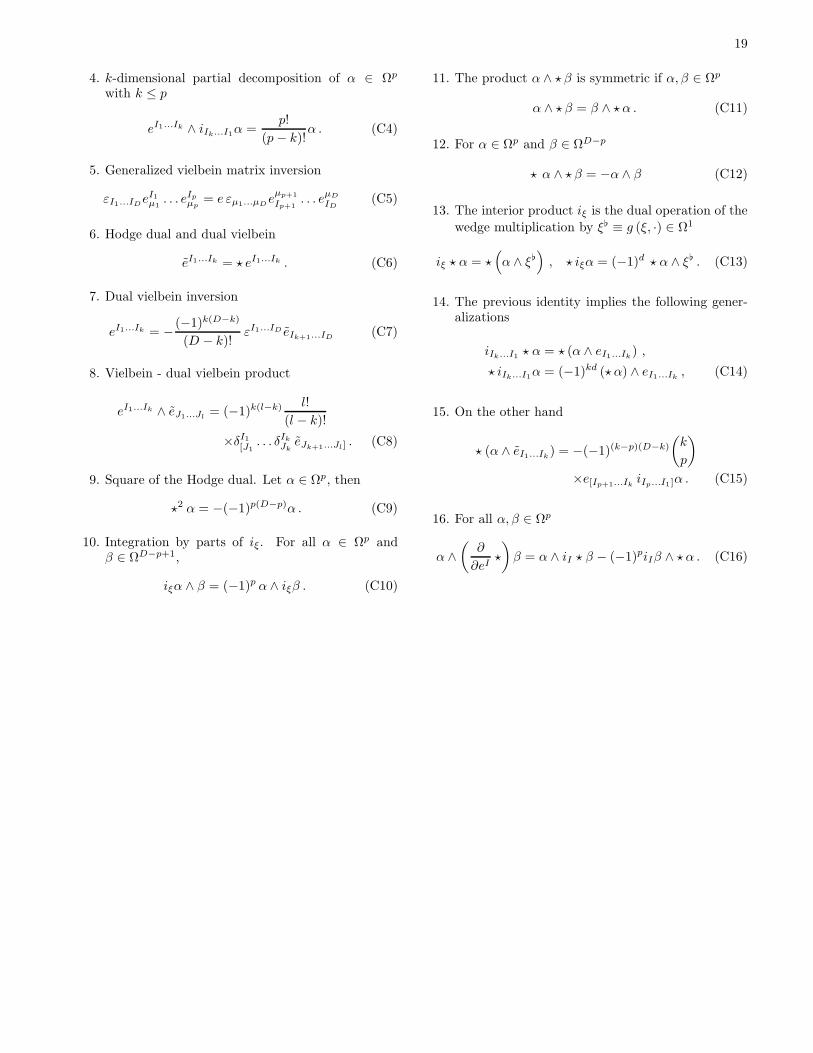
19

4. k-dimensional partial decomposition of α ∈ Ωp

with k ≤ p

eI1...Ik ∧ iIk...I1α =p!

(p− k)!α . (C4)

5. Generalized vielbein matrix inversion

εI1...IDeI1µ1. . . eIpµp

= e εµ1...µDeµp+1

Ip+1. . . eµD

ID(C5)

6. Hodge dual and dual vielbein

eI1...Ik = ⋆ eI1...Ik . (C6)

7. Dual vielbein inversion

eI1...Ik = − (−1)k(D−k)

(D − k)!εI1...ID eIk+1...ID (C7)

8. Vielbein - dual vielbein product

eI1...Ik ∧ eJ1...Jl= (−1)k(l−k) l!

(l − k)!

×δI1[J1. . . δIkJk

eJk+1...Jl] . (C8)

9. Square of the Hodge dual. Let α ∈ Ωp, then

⋆2 α = −(−1)p(D−p)α . (C9)

10. Integration by parts of iξ. For all α ∈ Ωp andβ ∈ ΩD−p+1,

iξα ∧ β = (−1)p α ∧ iξβ . (C10)

11. The product α ∧ ⋆ β is symmetric if α, β ∈ Ωp

α ∧ ⋆ β = β ∧ ⋆ α . (C11)

12. For α ∈ Ωp and β ∈ ΩD−p

⋆ α ∧ ⋆ β = −α ∧ β (C12)

13. The interior product iξ is the dual operation of the

wedge multiplication by ξ ≡ g (ξ, ·) ∈ Ω1

iξ ⋆ α = ⋆(

α ∧ ξ)

, ⋆ iξα = (−1)d ⋆ α ∧ ξ . (C13)

14. The previous identity implies the following gener-alizations

iIk...I1 ⋆ α = ⋆ (α ∧ eI1...Ik) ,⋆ iIk...I1α = (−1)kd (⋆ α) ∧ eI1...Ik , (C14)

15. On the other hand

⋆ (α ∧ eI1...Ik) = −(−1)(k−p)(D−k)

(

k

p

)

×e[Ip+1...Ik iIp...I1]α . (C15)

16. For all α, β ∈ Ωp

α ∧(

∂

∂eI⋆

)

β = α ∧ iI ⋆ β − (−1)piIβ ∧ ⋆ α . (C16)