Geometrical symmetry in the boundary element method

E L S E V I E R 0 9 5 5 - 7 9 9 7 ( 9 4 ) 0 0 0 3 9 - 5

Engineering Analysis with Boundary Elements 14 (1994) 229-238 © 1995 Elsevier Science Limited

Printed in Great Britain. All ri~ts r~rved 0955-7997/94/$07.00

Geometrical symmetry in the boundary element method

Jacques Lobry & Christian Broche Facult~ Polytechnique de Mons, Department of Electrical Engineering, Bd. Dolez, 31, 7000 Mons, Belgium

(Received 17 January 1994; revised version received 30 August 1994; accepted 7 September 1994)

Geometrical symmetry is found in many linear field problems. It cannot be intuitively taken into account for general excitation. A rationale is thus required and the group representation theory is the only valuable tool for this purpose. A theoretical description of this concept with application to the boundary element method is presented. Symmetrized kernels are derived in a systematic way. The general non-abelian case of symmetry is considered. Numerical results are presented and gains in CPU time and memory volume are measured to demonstrate the efficiency of the method.

Key words: Symmetry, g roup theory, bounda ry element method.

INTRODUCTION

In computational electromagnetics, problems that present geometrical and material symmetry are often met. It is easy to take advantage of this when the source fields and the boundary conditions share the symmetry, as is the case for an even or odd parity with respect to a reflection plane, but the intuitive reasoning fails for complex geometry and general excitation. How- ever, it is still possible to take full advantage of the symmetry thanks to the group representation theory which is a chapter of the general group theory, 1-3 well known by mathematicians and physicists, but, it seems, rarely taught to the engineers.

In this paper we first present a brief theoretical approach in a similar way as in an extended paper of Bossavit. 4 A basic description of the finite group concept is depicted in the point group context. Group actions on complex-valued vector space of functions introduce the representation theory where the main point is a decomposition theorem that is essential for our purpose. From the latter, exploiting the symmetry consists of reducing an original problem to a family of smaller ones defined on a reduced geometry - - a symmetry cell. A global solution is obtained from superposition of the partial results. Taking symmetry into account in a finite dement problem is very interesting since the only symmetry cell is to be discretized and the computational efforts (e.g. CPU time) generally grow much faster than the size of a problem. High gains are then expected. Up to now, few papers deal

with this method - - see, for example, the works of Bal- listi et al., 5 Bossavit, 6 Bonnet, 7 Allgower et al., s Lobry 9 and Lobry and Broche. ]°']]

Those concepts are applied to the boundary element method for the Poisson's problem. Integral formula- tions defined on a symmetry cell of the boundary of the domains under study are derived and symmetrized kernels appear in a natural way, coming from representation theory. The general non-abelian case of a symmetry group is considered so that we deal with coupled problems that are not obvious to determine, because of complicated reciprocal symmetry constraints. This is the case for geometry where rotational symmetry and mirror reflection planes coexist as in the dihedral groups. Other presentations 5'7's']°'11 exist in the literature. The method is implemented and some illustrative electrical examples are presented where the high efficiency of the method is demon- strated.

229

THE GROUP REPRESENTATION THEORY

First of all, we have to define the concept of finite group. We shall illustrate the definition with symmetry groups, but it is clear that the properties presented hereafter hold for any kind of finite group. The representation theory is then developed. The various theorems stated below are given with no proof for the sake of concise- ness. The reader should refer to specialized treatises 1-3 for more details.

230 J. Lobry, C. Broche

Table 1. Muldpliealien table of the group G

e f g

e e ff2 g s s g g g f

Finite symmetry groups

Definitions Let ~ be a spatial domain that presents some symmetry we describe by the isometrics g (rotations and reflections) that bring [2 into coincidence with itself. Those are transformations acting on points:

g: x---~gx

The isometrics form a finite group G = {e,f, g, . . .} , that is a finite set of elements on which a composition law ( . ) is defined so that:

(1) e E G : i fg E G,e.g = g (identity element) (2) i f g E G,g -1 E G : g . g -1 = e (inverse element) (3) i f g and h E G ,g .h E G

(G is closed under the law) (4) if f , g, h ~ G, ( f . g). h = f . (g. h) (associative law)

When the composition law happens to be commutative, the group G is said to be 'abelian'. In this paper, the general case of the non-abelian groups is considered. The number of elements in the group is the 'order of the group r~ ' . Any group may be defined by its 'multiplica- tion table' (Table 1).

An illustrative example is given in Fig. l(a) with the non-abelian dihedral group D 3. In this particular case, the isometries are e, r, r 2 (= r. r), s, sr, sr z, which respectively denote the identity, the +27r/3 and -21r/3 rotations and the three mirror reflections. This group is non-abelian since, for instance, s r ~ rs (=st2). From this example, we note that there exists a sub- domain C (symmetry cell) that regenerates f~ by the isometrics of G (Fig. l(b)):

f~ = U g c gEG

Some finite symmetry groups are frequently met in engineering applications. These groups are such that all the symmetry elements must intersect in at least one point; they are called 'point-groups'. Among them, we find:

(a) the group Cs that describes the symmetry about a mirror-reflection plane s;

(b) the cyclic group Cn that describes the rotational symmetry about an n-fold axis:

C n = {e,r, r2,r3, . . . ,r n-l}

where r is the elementary rotation of 21r/n, its order is n and it is abelian;

s

"sx x=e:~ 7-/ Ci:iiii:iiNiiiiiiiiii] \we

\ I --'Y'-. i / \ \ . / " I "'.. / / /

(a) (b)

Fig. 1. The d ihedra l g roup D 3.

(c) the dihedral group Dn that has an n-fold axis (rotations r k) and a system of n two-fold axes at fight angles to it (rotation srk):

D n = {e,r, r2, . . . , rn- l ,s , sr, sr2,...,sr n-l}

the order of the group is 2n and it is non-abelian for n > 2.

Properties of the finite groups Let us now examine some important Properties of the finite groups that we invoke in the representation theory.

(1) Conjugate class. A conjugate class K of a group G is a set of elements with respect to an equivalence relation:

Vg, h E K, g - h if 3x E G : g = xhx- 1

if G is made of k classes, we have

k k

G = U K i and N K i = ¢ i=1 i = l

Example. The group D 4 has five classes:

K e : {e}, Krl = {r, r 3} Kr2 = {r 2}

Ksl = {s, sr2}, Ks2 = {sr, sr 3}

For abelian groups, every element is in a class by itself. This is the case for the cyclic groups.

(2) Subgroups. A subgroup H of a finite group G is a subset of G that fulfills the following requirements:

(i) H C G (ii) Vg, h E H, gh E H

(iii) Vg E H,g -1 E H (thus e E H)

consequently, H is a group by itself.

(3) Direct product. Let Hi, H2 , . . . , Hn be n subgroups of G; G is the direct product of its subgroups:

G = H I ® H E ® . . . ® H n

if:

(i) NT=l Hi = {e}

Geometrical symmetry in the B E M 231

(ii) Vhi E Hi, I-I'~= 1 hi commutes (iii) Vg E G, 3!h i E Hi: g = 1-IT=l hi

The last property means that any element of G can be written in a unique way with h i. Moreover, we have

n

nG : H nHi i=1

Example. From the group D 6 and Cs, we form the group D6h = D 6 ® Cs, which consists of adding an horizontal symmetry plane to the isometries of the dihedral group D6. Its order is 24 (= 12 × 2).

Irreducible representations of a finite group

Definitions Consider a vector space V of complex-valued scalar functions on the affine space A3, where a scalar product (¢, ¢) is defined (¢ and ¢ in 1I) so that:

(i) (~b, ¢ ) = (¢ , ~b)* (ii) (),~b, ~b) = )t(~b, ¢)

(iii) (0, ~b) _> 0 (= 0 only if ~b = 0) (iv) (¢ + ~, ¢) = (¢, 4~) + (~, ¢)V4~, ~/,, ~ e V

then V is said to be 'unitary'. Consider now the set of linear operators O of V on to itself. Suppose V is an n- dimensional unitary space and let {el ,e2, . . . ,en} be a basis in V. The operator O may now be related to an n- by-n matrix representative D whose coefficients Dii verify:

Oe.i = £ D 0 ei'qj = 1 , . . . , n i = l

Let G = { e , f , g , h , . . . } be a finite symmetry group of order n~. We may assign operators Og to the elements g of G such that, for any function ¢ of V:

(og¢)(x) = ¢(g-lx)

In an equivalent way, we may write:

( Og~b)(gx) = ~b(x)

so that ¢ is transformed into the function ¢' = Og¢ where Og acts on the function ¢ as g acts on any point x of A3. To make clear, consider (Fig. 2) a trans- lation t of ¢ : R ~ R:

t : x - * tx = x + a

(Ot¢)(X) = ~b(t-lx) = ~b(x - a)

Operations g and Og are called 'group actions' on A 3 and V, respectively.

The main properties of the operators Og are:

(i) Vg, h E G, agO h = Og h (ii) Vg E G, Og-i = O~ 1

(iii) Oe = ! (identity operator)

The operators Og form a group G' isomorphic to G. By satisfying those properties, the mapping O is a

0 t

x :~+CL

t

R 1

Fig. 2. Group action Ot on a function ¢ : R ~ R.

'homomorphism' that we call here a 'linear representation' of the group G in the 'representation space' V. The matrix representatives D(g) of the operators Og also relate to a homomorphic mapping that is a 'matrix representative' of G and we have

D(g).D(h) = O(gh), D(g -1) = D - l ( g ) , D(e) = I

dim V = n is also the degree of the representation O (or D).

The matrix representatives D(g) and i f (g) of 0 in two different bases of V are such that

D t = TDT -1

where T defines the relation between the bases. The representations D and D' are then called equivalent.

0 is a 'unitary representation' of G if (Og¢,Og¢) = (¢,¢) for all g in G. So we have D(g) = D(g)

An important theorem in the representation theory is the Schur-Auerbach theorem: any representation of a finite group is equivalent to a unitary representation.

Analysis of representation and reducibility Let V (0 be a p-dimensional subspace of V; V (1) is said to be stable under a representation D of a finite group G only if

VX (1) E V (l), Vg E G : D(g)x (1) E V (1)

that is, V 0) is mapped on to itself by D(g) for all g in G. Moreover, there exists a stable (n -p)-dimensional subspace V (2) such that V = V 0) ~ V (2) (~ : direct sum).

If we can find an appropriate basis for V, the representation D may be written as

D ( g ) = ( D 0 ; (g) O ) } p D(2)(g) } n - p

The representation D is then said to be 'reducible'. The submatrices D (1) and D (2) are also shown to be linear representations of G in the subspaces V (1) and V (2), respectively, and D is the 'direct sum' of D (1) and D(2):

D = D (1) ~ D (2)

We can examine the representations D (0 and D (2) to see whether they in turn are reducible. They can be treated separately as we did with D. By continuing this pro- cedure, D is decomposed into elementary irreducible representations D (~). This leads to the Maschke theorem, i.e. every reducible representation of a finite group is decomposable, i.e. it can be split into the


Table 2. Irredncible r e l ~ m t i o m of Da

e r r ~ s sr s ?

1 1 2 1

(: a = e f2~/3.

1 1 1 1 1 1 1 -1 -1 -1

( ; a ~ ) (~0 0a) (0l 0 ) (0a ~0) ( ~ 0 )

direct sum of irreducible representations:

D = D 0) ~ D (2) ~ . . . (~ D (v) ~ . . . . ( ~ D (~) /J

where the stable subspaces V (~) of V are such that:

V = ( ~ V (~), dim(V (~)) = d,

In general, any irreducible representation may appear in several equivalent forms; we use the same symbol for them and we have the general symbolic statement:

D = ~ a~,D (') lJ

where a~ are positive integers. In engineering applications, most of the complicated

groups are cyclic and dihedral ones. The degrees do not exceed two. Notice, however, the particular but interesting case of the group Oh of all the isometrics of the cube that has 10 not-equivalent irreducible representations: 4 of degree 1, 2 of degree 2 and 4 of degree 3.

Fundamental theorems The following theorems are very useful in the derivation of the irreducible representations of finite groups:

(1) The number of not-equivalent irreducible representations of a finite group equals its number of classes.

(2) The sum of the squares of the degrees d~ of all the not-equivalent irreducible representations is equal to the order of the group:

k

.~=1

(3) Every degree d~ is a divisor of na. (4) All the irreducible representations of an abelian

group are of degree one. (5) The not-equivalent irreducible representations of

a direct product are given as the Kronecker-pro- ductsi" between the not-equivalent irreducible representations of its sub-groups: if

?1 n

G = ( ~ H i , VgGG, g = H g i , g i G H , i = 1 i = 1

then:

= o ? > ( g , ) , = l

?The Kronecker-product of the matrices A(nA) and B(nB) is C(n A . na ) where cij,kl = aa . bfl.

Consequently, the degree of D (V) is the product of the partial degrees, and the number of irreducible representations of G is the product of the numbers of those of the Hi.

(6) Let D (~) and D (J') be two not-equivalent irreducible representations of a group G = { e , f , g , h , . . . } (order no), of degree d~ and d~,, respectively. Consider the d~(~,) n¢-dimensional vectors:

rnO') (') (',') v-'it (e),Oil ( f ) ,Di t (g),. . .] i , l = 1,. . . ,d~

l j , m : 1, ,a.

If the representations are unitary, we have an orthogonality relation with respect to the following scalar product:

d~ E (~) (~}* - - D . (g)D); , (g) = nG gEG

Thus, each irreducible representation D (") provides d~ vectors which are orthogonal to one another and to the d~ vectors of the representation D (~'). From the Schur-Auerbach theorem, it yields that this property is general.

(7) Many applications in physical sciences involve only the traces or characters Xg = EiDii(g) of the (reducible or not) representations of a finite group. Some properties of the characters are:

• two equivalent representations have the same characters, and inversely;

• the characters of two unitary irreducible representations D (~) and D (~') verify the orthogonality relation:

1 ~ ~(~)~(i,) 6~, Ag Ag

nG gGG

As an example, the irreducible representations of the dihedral group D3 are given in Table 2; the reader is invited to test the previous theorems.

The irreducible representations of a group are always given up to an isomorphism. For instance, the complex representation of degree 2 D (s) of the group D3 is equivalent to a real one D '(s) that can be found by choosing a transformation T such that

1


e r

Tabl~ 3. Real re~tion D (s) of Ds

t 2 s sr sr ~ (1 ?) (1o o) , Dr(3) ~ _

2 2

/ 1 2~3__~)V~2 ( 0 1 ) 0 1 __ ( lv/32 : ] ( 1 ____~)V/32

2 2 2

then, frO) is given by

D'<3)(g) = T.D<3)(g). T -1 Vg • G

and the related matrices arc those of Table 3. Now comes the main point of the theory for the

exploitation of geometrical symmetry in field problems.

The orthogonal decomposition theorem Given a unitary irreducible representation D (~) of a group G in a vector space V. Wc define the following linear operators called 'projectors':

p!.~) _ du Z D~ v)*(g)Og (i,j = 1, . . . , du) tj nG g~G

there are d 2 projectors in every representation. By sum- ruing the d. operators p~V), we obtain the Reynolds' projector p('v):

= Z + E u+.,, - - A,g ~ g j = l nG g~G

From those definitions, we may now express the orthogonal decomposition theorem:

(1) The projectors P(~) map the space V on to subspaces V (~) called G-isotypic components of V:

V(V) - p(v) V (u = I , . . . , k)

and

V = ~ V (v) 1/

(2) The operator PlY ) is zero on V (~) when # # u and map V on to ~ ) :

Vy(~) = P~')V ( u = 1 , . . . , k , j = 1, . . . ,dr)

Moreover

J

The subspaces V/(v) are mutually orthogonal since the projectors P~) are orthogonal:

C>Pl; > = + , : , , 6 ~'

Finally, V is decomposed into the Y~):

(3) The operator p~v)is zero on "v~V~(U)when # ~ ~ and k ~ j; it maps isomorphically I"~ ) on to V~ ).

Decomposition of a function defined on a symmetrical domain From a practical point of view, we now examine the incidence of the latter theorem conducting the decomposition of a function ¢ of the functional space V. ¢ is defined on a symmetrical domain f~ of which the isometries form a group G. Figure 3 illustrates a domain f~ that presents the two symmetry groups C3 (abelian case) and D3 (non-abelian case) with a symmetry cell C in each case.

From point (2) of the theorem, the projectors p~V) transform ¢ into some functions ¢~):

~'~ = 6 ~ where 4 v~ • v~ ~ (i)

such that k a~

= E Z 4 + (2> u = l j = l

For each function ¢(~) we can find ( 4 - 1) 'partner functions' ,~!.~) coming from the ( d , - 1) projectors r q

p!.U) (i ¢ j ) :

¢~v) = -11 p!'~) '~!'~)-n = P~")¢ (3)

Hence, we define a set of d, functions for given u and j that is called a 'u-symmetric set':

{¢~') : i = 1,. . . , dr}

Such a set satisfies the necessary and sufficient condition: av

o:(,;'= ~ ,,~+,.,.~v) "li ~6:V'lj Vg • G (4) 1=1

This relationship shows that the only restriction of the functions ~!.~) on the symmetry cell C of the domain fl

S

~/ i!iii',iiii+i!iiii!iiiiiiiii~ii~iiiiiiiii~iiiii'i!~t .~+ / !iiii iii! ,T, ~. l:!!ii: :!:i:i:ii:i:i!i:i!:?

ST ~ ST 2

Fig. 3. Symmetrical domain with (a) an abelian group and (b) a non-abelian group.


is sufficient to regenerate all of them entirely on the whole domain. In particular, this is the symmetry prop-

of the components ¢~Jf). Notice that an abelian e r t y case provides us components ~b (~) ( j = 1) that are symmetrical by themselves whereas in the non-abelian case the

q~l~ ') need other functions in order to be components known everywhere on f~. The latter case suggests some coupling as we will see in the next section. In general, any function q~ gives rise to Ed 2 = ne linearly independent components r~!. ~) sometimes called 'Fourier compo- r l j nents' of ~b. The statement (1) is the 'Fourier analysis' of function ~b whereas relation (2) is its 'Fourier synthesis'.

How to apply the above concepts to a finite element method is easy to guess. Starting from an original problem described by a set of equations defined on a domain f~ with symmetry, we have to determine a symmetry cell and to solve on it for the source fields or boundary conditions derived from each irreducible representation. The overall solution is finally obtained from superposition and symmetry operations. We now describe the exploitation of symmetry in the boundary element method.

THE BOUNDARY ELEMENT METHOD WITH SYMMETRY

Consider the Poisson's problem defined on a two- dimensional (2-D) domain f~ with geometrical symmetry (Fig. 4):

verb = f in f~ (5)

Some boundary conditions are imposed on Of~ for ~b (on Oleo) and its normal derivative (on Of~q). The source term f is assumed harmonic, i.e. V2f = 0, but it does not share any symmetry with fL

Recall that the Poisson's eqn (5) can be written in the following boundary integral formulation 12 for any point i of f~:

~ { O~ , OW i "~ CiOi )dr

(fOvi O f ) d F (6) - joa On-Vion

where the weighting functions ('kernels') w~ and v~ are such that

1 1 w,(x) = ln-d(?,x)

vi(x) - d(i, x) 2 [1 - lnd(i, x)] 8~r

and ci equals one if i is in f~\Of~ or a/27r if i is on 0Q (Fig. 4). For a nonhomogeneous domain, the above formulation is valid in each homogeneous part, and suit- able continuity relations across interfaces have to be added for the uniqueness of the solution. Generally, at

this stage, a discretization of the boundary 0fl into elements together with an appropriate approximation of the unknown functions (~b and its normal derivative) are achieved. That leads to a linear system of equations to be solved. However, when the domain exhibits symmetry, it is interesting to go further in the development of the boundary integral formulation.

Consider now the symmetry of the domain 9t in Fig. 4. It is described by a group G of order na and we may choose a symmetry cell F of 0f~ such that (Fig. 5):

0f~ = U gF (7) gEG

Henceforth, we let aon(d~,wi) and bo~(f, vi) denote respectively the first and second integrals of the right- hand side of the relation (6) for the sake of con- ciseness. Exploiting the property (7), we may write the statement:

a~(cp, w,) = ~ ag-tr((p , wi) gEG

= y ~ ar(Og4~, Ogwi) (8) gEG

and a similar expression for boa(f, vi). By using the theory described above, the unknown function 4~ and the source term f are decomposed as/in eqn (1). Then, introducing each component ~b~f and f~ ) ( v = 1 , . . . , k , j = 1 , . . . , d , ) in the formulation (6), substituting the integral identity (8) and using u- symmetric conditions (4), we obtain:

Ci(9~; )(i) = Z aF(OgO~ v)' Ogwi) gEG

"~- Z br(Ogfj~ v)'Og'Ui) gEG

= E ar ~0" klslW'lJ ' OgWi gEG l=1

+ br ~0 lg)Yt) , Ogvi " l = 1

Z (,1 (~) = a r Oij , Dtj (g)OgWi l=1 \ gEG /

a, nG

= ~ E " "t'(v) " (u)" ,,r~'etj , "O,i ) I=1

a~ nG

urlJ~ , vO,i ) I = l

Finally, the following d~ problems are m be solved for each irreducible representation u = 1 to k and j = 1 to


0 Q ,

Fig. 4. The 2-D Poisson's problem on a symmetrical domain.

Fig. 5. Symmetry cell of Off.

Gain o f the method

d~ and i is on F:

t=l \"o . On

~vo, i ''J q + -~ t= l On

a~ (~)* \ _ _ _ ~(~)v"O,i

tj On ,] dF

.qo,(v)* \

On ] dF (9)

Each problem involves v-symmetric components coupled with the reciprocal constraints (eqn (4)). We note that

kernels' wl~v,_ and v~,~ ~ have been intro- s o m e 6 Syl~nl~et r ~ d

duced from the symmetry operations:

(~) P!~,)wi(x) = d~ (~). 1 1 WiLl(X) = " ' " ~o E Do (g)-f~rlrln'd(i,g-lx)

g E G

and a similar expression for • (~) vq, r Thus, the original problem defined over the entire

boundary o ~ has been replaced by an equivalent set of d~ subproblems coupled by constraints defined over the reduced open boundary F. The discretization of the boundary into linear elements, together with an appropriate approximation of the unknown functions

f~) (qt~ and its normal derivative), leads to some linear sys- tems of equations. A solution method like the Gaussian elimination can be used.

Note that the symmetry should also be material and not only geometrical for an adequate treatment.

Taking again our group D3 as an example, the problems related to the two first irreducible representations (of degree one - - Table 2) are readily built by using the kernels w~ l) and wl 2), where i is any node of P. Concerning the third representation (degree 2), the choice of i on P and sP, for instance, leads to the required number of independent equations for the two coupled problems ( j = 1 and 2). This is equivalent to taking the u-symmetric sets:

,,(3) ~(3) l and ~(3) ~(3) l V i E F "~ll, i ' "v21,iJ t ' ~12 , i ) "~22,iJ

as test functions in problems (9) for j equals 1 and 2, so that the two problems differ from the right-hand side and only one factorization is then performed.

In the abelian case, we have already noticed that the number of irreducible representations is equal to the order n¢ of the group and they are all of degree one. Let N be the size of the global problem - - the number of nodes - - then the time required is roughly:

T = O(N ~) (1.5 < e < 3)

When symmetry is considered, the time T reduces to Tsym:

[ T, ym = O nc =

so that a gain of about n~- l should be expected. It may be very high if E and n~ are high. When dealing with non-abelian groups, this gain is smaller because of the coupled problems. Let us examine the execution time more precisely to see what exactly happens.

The execution time expressed in terms of assembling and solving times/'ass and Tsolv without any symmetry consideration is of the form:

T = Tas s + Tsolv = O ( a N 2 +/3N ~) + o(N)

where a and/3 are constants. When we take advantage of the symmetry, the execution time of our algorithms is found to be: t°

= 0 0~-- aIN 2

+ o(N)

where a' ,~, a/18. Normally we have Tsym(n~)< T so that we may

define a 'computational gain' 7 equal to the ratio T/Tsym(na) > 1. Given a value of ha, it can be easily proved that Tsy m is minimum when the original group is abelian:

Tsym abel(riG) < Tsym nonabel(nG) (10)

moreover, Tsym abel decreases with n~ so that, in particular:

Tsym abel(nG) < Tsym abel(n~/2) (I I)

As we said above, the non-abelian groups that frequently occur are dihedral ones D,(n6 > 2); they include the abelian cyclic groups C, of half order.


50cos~

100

15cos~ (a)

0

5 0s i n ~

(b)

~Ssin~

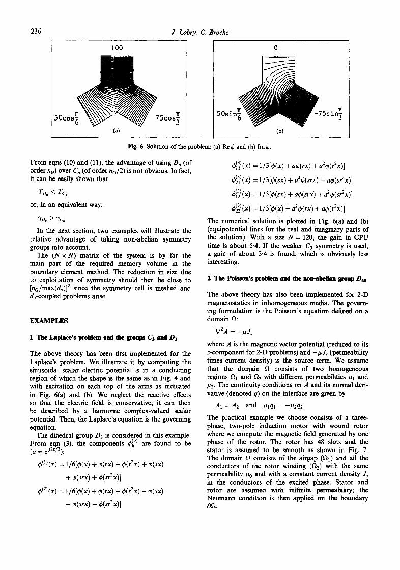
Fig. 6. Solution of the problem: (a) Re 0 and (b) Im 0.

From eqns (10) and (11), the advantage of using Dn (of order n~) over C, (of order no~2) is not obvious. In fact, it can be easily shown that

TD, < Tc.

or, in an equivalent way:

TO, >7C,

In the next section, two examples will illustrate the relative advantage of taking non-abelian symmetry groups into account.

The (N × N) matrix of the system is by far the main part of the required memory volume in the boundary element method. The reduction in size due to exploitation of symmetry should then be close to [ne/max(d~)] 2 since the symmetry cell is meshed and d~-coupled problems arise.

EXAMPLES

1 The Laldaee's ~ and the groups C3 and Da

The above theory has been first implemented for the Laplace's problem. We illustrate it by computing the sinusoidal scalar electric potential ~ in a conducting region of which the shape is the same as in Fig. 4 and with excitation on each top of the arms as indicated in Fig. 6(a) and (b). We neglect the reactive effects so that the electric field is conservative; it can then be described by a harmonic complex-valued scalar potential. Then, the Laplace's equation is the governing equation.

The dihedral group D 3 is considered in this example. &!.~) are found to be From eqn (3), the components ~,,j (a= eJ2~r/3):

¢(1)(x) = 1/6[O(x) + ck(rx) + ok(rEx) + O(sx)

+ fb(srx) + c~(sr2x)]

~b(2)(x) = 1/6[~b(x) + dp(rx) + ~p(r2x) - (b(sx)

- (p(srx) - O(sr2x)]

= 1/3[(b(x) + afb(rx) + a2(b(r2x)]

= 1/3[~p(sx) + a2cb(srx) + a~b(sr2x)]

= 1/3[(b(sx) + a~p(srx) + a2~b(sr2x)]

= 1/3[~b(x) + a2~p(rx) + aq~(r2x)]

The numerical solution is plotted in Fig. 6(a) and (b) (equipotential lines for the real and imaginary parts of the solution). With a size N = 120, the gain in CPU time is about 5.4. If the weaker C3 symmetry is used, a gain of about 3.4 is found, which is obviously less interesting.

2 The Poison's problem and the non-abelin group Da

The above theory has also been implemented for 2-D magnetostatics in inhomogeneous media. The governing formulation is the Poisson's equation defined on a domain f~:

V2A = -#J~

where A is the magnetic vector potential (reduced to its z-component for 2-D problems) and -#J s (permeability times current density) is the source term. We assume that the domain f~ consists of two homogeneous regions f~! and f12 with different permeabilities #1 and #2. The continuity conditions on A and its normal derivative (denoted q) on the interface are given by

A 1 = A 2 and # l q l = --/~2q2

The practical example we choose consists of a three- phase, two-pole induction motor with wound rotor where we compute the magnetic field generated by one phase of the rotor. The rotor has 48 slots and the stator is assumed to be smooth as shown in Fig. 7. The domain [2 consists of the airgap (ill) and all the conductors of the rotor winding (f12) with the same permeability P-0 and with a constant current density Js in the conductors of the excited phase. Stator and rotor are assumed with inifinite permeability; the Neumann condition is then applied on the boundary 0f~.

Geometrical symmetry in the BEM 237

stator( ~--'~ ) c o r e ~ alrgap(fll)

UCtOTS

(~2)

Fig. 7. Geometry of the induction motor.

The symmetry group is the non-abelian group D48 of order 96; it has 27 irreducible representations: 4 of degree 1 and 23 of degree 2. In this situation, the excitation ,Is gives rise to 24 components J~l and ~=22 T(v) coming from 12o f the 23 representations of degree 2. Hence, 24 coupled subproblems are to be solved on 1/96th of the geometry. On the other hand, the excitation exhibits some obvious symmetry with respect to the rotor so that the problem could be solved on only a quarter of it. So a comparison between this classical approach and our method is the right way to measure unbiased performances with the proposed example. The solution obtained from both methods is illu- strated by the A-lines (identical to the flux lines) in Fig. 8. They result from a postprocessing computation of the potential A inside the rotor core after solving the Poisson's problem on fL By measuring the execution times required for solving the problem in each case, we find 10 rain 45 s for the first and only 45 s for the second. Hence, a gain of about 14 (!) that proves the high efficiency in taking advantage of the full symmetry of the problem. The size of the problem is N = 696 for a quarter of the machine. The reduction

Pig. 8. Flux lines in a quarter of the rotor core.

in memory volume is about n~/64 = 1.5, which is much lower than the theoretical value of n2o/64. This important sacrifice is due to some extra data storage required to minimize greatly the execution time with our algorithm. In general, the user has to manage a compromise between the size and the computation time.

CONCLUSION

In this paper we have presented a rationale for taking advantage of geometrical symmetry in field problems. The group representation theory was briefly presented from the finite group concept. Fundamental theorems of the representation theory have led us to an orthogonal decomposition that is the crucial point for our purpose. Exploiting the symmetry then consists of reducing an original problem to a family of smaller ones defined on a symmetry cell of the initial domain. A global solution is obtained from superposition of the partial results. The method has been applied to the 2-D boundary element method where symmetrized kernels were derived in a natural way. Some examples have pointed out the efficiency of the method, which leads to substantial computational cost savings.

REFERENCES

I. Hamermesh, M., Group Theory. Addison-Wesley, Massa- chusetts, Palo Alto and London, 1964.

2. Serre, J.-P., Reprdsentations Lindaires des Groupes Finis. Hermann, Pads, 1971.

3. Jansens, L. & Boon, M., Theory of Finite Groups, Applications in Physics. North-Holland, Amsterdam, 1967.

4. Bossavit, A., Symmetry, groups, and boundary value problems. A progressive introduction to non-commutative harmonic analysis of partial differential equations in domains with geometrical symmetry. Comput. Meth. Appl. Mech. Engng, 1986, 56, 167-215.

5. Ballisti, R., Hafner, C. & Leuchtman, P., Application of the representation theory of finite groups to field computation problems with symmetrical boundaries. IEEE Trans. Magn., 1982, 18, 584-7.

6. Bossavit, A., The exploitation of geometrical symmetry in 3-D eddy-currents computation. [EEE Trans. Magn., 1985, 21, 2307-9.

7. Bonnet, M., On the use of geometrical symmetry in the boundary element methods for 3D elasticity. In Boundary Element Technology, Vol. VI, ed. C. A. Brebbia. Computational Mechanics Publications, Southampton, 1991, pp. 185-200.

8. Allgower, E. L., Bthmer, K., Georg, K. & Miranda, R., Exploiting symmetry in boundary elements. SIAM J. Num. Anal., 1992, 29, 534-52.

9. Lobry, J., Symttries et 616merits de Whitney en Magntto- dynamique tridimensionnelle. Phi) thesis, FPMs, 1993.

10. Lobry, J. & Broche, C. Exploitation of the geometrical


symmetry in the boundary element method with the group representation theory. IEEE Trans. Magn., 1994, 30, 118- 23.

11. Lobry, J. & Broche, C., Non-abelian symmetry in the BEM for an induction motor. In Boundary Element Technology, Vol. VIII, ed. H. Pina & C. A. Brebbia.

Computational Mechanics Publications, Southampton, 1993, pp. 137-46.

12. Brebbia, C. A. & Dominguez, J., Boundary Elements - - An Introductory Course, 2nd edn. Computational Mechanics Publications, McGraw-Hill, New York, 1992.

Geometrical symmetry in the boundary element method

Documents

Transcript of Geometrical symmetry in the boundary element method