a simulative study on geometrical misalignments - JSSS

J. Sens. Sens. Syst., 11, 171–186, 2022https://doi.org/10.5194/jsss-11-171-2022© Author(s) 2022. This work is distributed underthe Creative Commons Attribution 4.0 License.

Acceptance and reverification testing for industrialcomputed tomography – a simulative study on

geometrical misalignments

Florian Wohlgemuth1, Tino Hausotte1, Ingomar Schmidt2, Wolfgang Kimmig3, andKarl Dietrich Imkamp3

1Institute of Manufacturing Metrology (FMT), Friedrich-Alexander-Universität Erlangen-Nürnberg (FAU),Nägelsbachstraße 25, 91052 Erlangen, Germany

2Werth Messtechnik GmbH, Siemensstraße 19, 35394 Gießen, Germany3Carl Zeiss Industrielle Messtechnik GmbH, Carl-Zeiss-Str. 22, 73447 Oberkochen, Germany

Correspondence: Tino Hausotte ([email protected])

Received: 17 November 2021 – Revised: 14 May 2022 – Accepted: 16 May 2022 – Published: 16 June 2022

Abstract. Acceptance and reverification testing for industrial X-ray computed tomography (CT) is described indifferent standards (E DIN EN ISO 10360-11:2021-04, 2021; VDI/VDE 2630 Blatt 1.3, 2011; ASME B89.4.23-2020, 2020). The characterisation and testing of CT system performance are often achieved with test artefactscontaining spheres. This simulative study characterises the influence of different geometrical error sources – orgeometrical misalignments – on these sphere measurements. The two measurands on which this study focusesare the sphere centre-to-centre distances and the sphere probing form errors.

One difference between the current draft of the ISO 10360-11 standard (E DIN EN ISO 10360-11:2021-04,2021) and the VDI/VDE standard 2630 part 1.3 (VDI/VDE 2630 Blatt 1.3, 2011) as well as the ASME standardB89.4.23 (ASME B89.4.23-2020, 2020) are the differences for the sphere centre-to-centre distances that need tobe measured. The VDI/VDE standard and the ASME standard require measurements of these kinds of distancesof up to 66 % of the possible maximum distance within the measurement volume, while the ISO draft asks formeasurements of up to 85 % of the possible maximum distance. This requirement needs to be considered inconnection with the maximum permissible error (MPE) specification for these sphere distance measurements.This MPE should be specified as a linear function of the nominal distance or a constant value or a combinationthereof (compare definition 9.2 of ISO 10360-1:2000+Cor.1:2002 (DIN EN ISO 10360-1:2003-07, 2003)), andthus, the linearity of the length-dependent maximum measurement error of the sphere distance measurementsis of interest. This simulative study inspects to what extent this linearity can be observed for CT measurementsunder the influence of different geometric errors. Further, the question is whether measurement lengths above66 % necessitate a change in the MPE specification. Thus, an automatic identification of cases that might affectthe MPE specification is proposed, and these cases are inspected manually.

A second aspect of this study is the impact of geometrical misalignments on the probing form errors of ameasured sphere. The probing form error also needs to be specified. Thus, whether and how it is influenced bythe misalignments is also of interest.

Based on our simulations, we conclude that probing form errors and sphere centre-to-centre distances of up to66 % of the maximum possible measurement length within the measurement volume are sufficient for acceptancetesting concerning geometrical misalignments – each geometrical misalignment can be detected well with at leastone of these two measurands.

Published by Copernicus Publications on behalf of the AMA Association for Sensor Technology.

172 F. Wohlgemuth et al.: Acceptance and reverification testing for industrial CT

1 Introduction

Acceptance and reverification testing for industrial X-raycomputed tomography (CT) is important for users and man-ufacturers alike as it is used to test technical specificationsthat are contractually guaranteed. The testing procedure isdescribed in different standards (E DIN EN ISO 10360-11:2021-04, 2021; VDI/VDE 2630 Blatt 1.3, 2011; ASMEB89.4.23-2020, 2020). The characterisation and testing ofCT system performance are often achieved with test arte-facts containing spheres. Measurands in acceptance testingthat we inspect in this paper are the errors in centre-to-centredistances of the spheres (SD errors) as well as the sphereprobing form errors. This simulative study characterises theinfluence of different geometrical misalignments of the CTacquisition geometry on these sphere measurements. Onedifference between the current draft of the ISO 10360-11standard (E DIN EN ISO 10360-11:2021-04, 2021) and theVDI/VDE standard 2630 part 1.3 (VDI/VDE 2630 Blatt1.3, 2011) as well as the ASME standard B89.4.23 (ASMEB89.4.23-2020, 2020) are the differences for the spherecentre-to-centre distances that need to be measured. Both theVDI/VDE standard and the ASME standard require measure-ments of up to 66 % of the possible maximum distance withinthe measurement volume, while the ISO 10360-11 draft asksfor measurements of longer distances (current draft: mea-surements of up to 85 %). In the usual case of a cylindri-cal measurement volume, the maximum distance within themeasurement volume is the diagonal. The requirement tomeasure up until certain lengths needs to be considered inconnection with the maximum permissible error (MPE) spec-ification for these sphere distance measurements. This MPEshould be specified as a linear function of the nominal dis-tance or a constant value or a combination thereof (comparedefinition 9.2 of ISO 10360-1 (DIN EN ISO 10360-1:2003-07, 2003)), and thus, the linearity of the length-dependentmaximum measurement error of the sphere distance mea-surements is of interest. This simulative study inspects towhat extent linearity can be observed for CT measurementsunder the influence of different geometric errors. Further, thequestion is whether measurement lengths above 66 % neces-sitate a change in the MPE specification. Thus, an automaticidentification of cases that might affect the MPE specifica-tion is proposed, and these cases are inspected manually.

A second aspect of this study is the impact of geometri-cal misalignments on the probing form errors of a measuredsphere. The probing form error does also need to be speci-fied and can also indicate geometrical misalignments. Thus,whether and how it is influenced by the misalignments is alsoof interest. Generally, it will suffice that either probing formerrors or sphere centre-to-centre distances are sensitive to aspecific geometric misalignment.

Similar work has been performed by Muralikrishnan et al.(2019a, b, c) and Jaganmohan et al. (2020). The differ-ence between that study and the work presented here is that

the study by Muralikrishnan et al. (2019a) employs a self-developed geometric forward- backward projection simula-tion of the sphere centre points, while we use the radio-graphic simulator aRTist 2 by the German Federal Institutefor Materials Research and Testing (BAM) (see, for example,Bellon et al., 2012) and simulate realistically sized spheres.The radiographic approach also means that our simulationsproduce projection data which are subsequently processedwith volume reconstruction and surface point determinationthe same way real CT data are processed. A further differ-ence is that Muralikrishnan et al. (2019a, b, c) and Jagan-mohan et al. (2020) had the goal of finding the most sensi-tive measurement distances for different single geometric er-rors, while we want to analyse the distribution of the spherecentre-to-centre distance errors with respect to the nominaldistance and inspect probing form errors. Another extensionin comparison the work of Muralikrishnan et al. (2019a, b, c)and Jaganmohan et al. (2020) is that in our analysis, we wantto include simulations with combinations of multiple geo-metric misalignments as real CT systems will also show acombination of these.

2 Linearity and MPE-relevant behaviour

The MPE can be specified as a linear function of the mea-surement length, a constant value or the minimum of both.In agreement with VDI/VDE 2630 Blatt 1.3 (2011), we dis-regard the option of constant values for SD errors in dimen-sional computed tomography. It is well known that transla-tions of rotary table, source and detector in the beam direc-tion lead to scaling errors that increase linearly with the nom-inal length (as shown by simulation results in Sect. 4.1). As-suming a linear MPE specification, the decision as to whetherlong sphere distances need to be measured depends on howthe maximum errors in these distance measurements increasewith the nominal sphere distance. We can imagine four dif-ferent patterns for the SD errors (compare Fig. 1). First, theycan increase linearly with the sphere distance. Second, theycan increase roughly linearly with the sphere distance, mean-ing that there are two parallel linear functions within whichall data points lie. Third, they can increase with the nominaldistance less than a linear function would (e.g. with a square-root behaviour), and fourth, they can increase more than alinear function would (e.g. with a parabolic increase). Ofthese four cases, only the case of “more than linear” increaseneeds to be considered relevant in the context of the MPEspecification, as an MPE based on data for lower lengthsmight not be valid any more at long lengths. This will nothappen in the other three cases.

In the following, we will often use the Pearson correlationcoefficient ρ (or the square root of the coefficient of determi-nation R2 of a linear fit to the data; see Fahrmeir et al., 2009)to gauge linearity. While a value of |ρ| ≈ 1 indicates linearbehaviour, a value below 1 does not allow for any statement

J. Sens. Sens. Syst., 11, 171–186, 2022 https://doi.org/10.5194/jsss-11-171-2022

F. Wohlgemuth et al.: Acceptance and reverification testing for industrial CT 173

Figure 1. Four different patterns for the SD errors can be imagined. The pattern in plot (a) illustrates strictly linear behaviour, indicated bya correlation coefficient of ρ = 1. The pattern in plot (b) illustrates a behaviour that is roughly linear in the sense that there are two parallellinear functions within which all data points lie. The pattern in plot (c) illustrates an increase that is less than linear; i.e., the increase ofthe measurement deviation with the nominal length is less than linear. The pattern in plot (d) indicates more than linear behaviour. Thislatter behaviour is the only one we would deem relevant for the MPE specification as an MPE limit constructed using points up to a certainpercentage might easily be exceeded by points at a higher percentage. The plots show that while the correlation coefficient ρ can detectstrictly linear behaviour, it is not sufficient for deciding whether or not a given pattern would be relevant regarding the MPE specification.

about the kind of non-linearity the data exhibit. Therefore,any value clearly different from 1 does not allow for any con-clusion on whether the underlying data would be relevant inthe context of a linear MPE specification or not. Therefore,we propose a further analysis method in Sect. 5 which pro-vides an automated criterion for cases with |ρ| 6= 1.

3 Simulative setup

Section 3.1 describes the simulation parameters and geome-try, including the geometric misalignments that can be simu-lated. Section 3.2 describes the artefact geometry that is usedfor this study. Section 3.3 describes the data processing afterthe radiographic simulation.

3.1 Simulation parameters and geometry

For the simulation, we used aRTist 2 by the German Fed-eral Institute for Materials Research and Testing (BAM) (see,for example, Bellon et al., 2012) in version 2.10.0. To min-imise the influence of other error sources, the simulationsare monochromatic (200 keV), without scatter, and the detec-

tor is perfectly linear with a maximum grey value of 60 000at free beam. The simulation artefact material is set to alu-minium. The detector of the acquisition setup has a pixelpitch and unsharpness of 0.4 mm and is noise-free. The de-tector is positioned 1000 mm from the point source and theobject at 250 mm, resulting in a magnification of 4. Thedetector is 600 mm wide and 500 mm high (equivalent to1500 pixels× 1250 pixels). The resulting half-cone beam an-gle is 16.7◦. A total of 1500 projections on a regular circletrajectory are simulated. The measurement volume, i.e., thecylinder whose content is completely projected onto the de-tector in all projections, has a diameter of 121.27 and a heightof 113.62 mm. Its diagonal (the maximum distance withinthe cylindrical measurement volume) is 166.18 mm long. TheSTL (Standard Triangle Language file format) model of thesimulation artefact is positioned with its bounding box cen-tre at x = y = 0 mm and with a distance of 250 mm to thesource along the z axis (see Fig. 2 for the coordinate systemdefinition). In a real CT, the rotary table should not be pro-jected onto the detector. The pivot point of the rotation axisis therefore located 77.125 mm below the central beam axis(translated downwards in the negative y direction). This will

https://doi.org/10.5194/jsss-11-171-2022 J. Sens. Sens. Syst., 11, 171–186, 2022


become relevant when misalignments are considered. Theacquisition geometry is illustrated in Fig. 2.

aRTist 2 can simulate projection-wise geometric errors ofthe acquisition geometry (compare, for example, Wohlge-muth et al., 2018, 2020). The original implementation ofaRTist 2 was modified slightly for the purpose of this study.The following modifications are possible for each projection(in this order):

– Detector position and orientation, source position androtation axis position are modified (with respect to theirundistorted value) according to values for this projec-tion from an input file. If vud is the undistorted (nom-inal) parameter value (3D vector), then the parametervalue v(j ) for projection j results from a displacementvalue δ(j ) according to

v(j )= vud(j )+ δ(j ). (1)

– The value for the direction of the rotation axis for thisprojection (again from an input file) is applied. The ro-tation axis direction is encoded as a 3D unit vector inaRTist; thus, the input file contains one such unit vectorn(j ) for each projection j which is applied in this step.

– The measurement object is translated and rotated to ac-count for the movement of the rotation axis (the con-nection between measurement object and rotary table isassumed to be rigid). This means that the translation ofthe rotation axis position between projection j − 1 andj is applied also to the object and that the object is thenrotated to account for the different orientation betweenrotation axis direction n(j−1) from projection j−1 andprojection axis direction n(j ) from projection j .

– After image acquisition, the object is rotated by the an-gular increment value for this projection (again from aninput file) around the current rotation axis with directionn(j ) and position for projection j .

These modifications are used to represent actual possiblegeometrical misalignments of an industrial CT, described inthe following. Without reference to the specific machine per-formance of a specific CT, it is unclear what good numericalvalues for these geometrical misalignments are. We used es-timated values as described below, but we did also vary thenumerical values during the study (see Sect. 4).

– Detector position perpendicular to central beam axis (xand y axis). For the detector translation perpendicular tothe central beam axis (x and y direction), we assume amaximum error of 2 mm.

– Detector position along beam axis (z axis). A detectortranslation in the beam direction can be detected as ascaling error. We assume that one of the most simple

calibration procedures is to use two spheres with cali-brated distance and project these onto the detector. Thedistance between the projected sphere centres dividedby the calibrated distance can be used to determinethe magnification. If we assume that the magnifica-tion is M = 4, the calibrated distance is 10 mm± 1 µmand the centre-to-centre distance determination on theprojection is possible with half pixel pitch accuracy,then the relative error of the source detector distance isaround 5× 10−3. Assuming that this is the uncertaintyin source–detector distance, this translates into a maxi-mum detector misalignment in beam direction (z direc-tion) of 3.75 mm.

– Detector orientation. With a simple spirit level, a mea-surement accuracy of 0.057◦ can be achieved. There-fore, we assume a maximum detector tilt in all direc-tions of this measurement accuracy.

– Source position. For the translation perpendicular to thebeam axis (x and y axis), we assume – as with the de-tector – a maximum error of 2 mm. The beam axis (zaxis) translation induces – as with the detector – a scal-ing error. With the same estimation as for the detector,we used a maximum error of 0.65 mm in the beam di-rection.

– Rotation axis tilt. Like Muralikrishnan et al. (2019a) andMuralikrishnan et al. (2019b), we use a maximum errorof 0.2◦ tilt in all Cartesian directions.

– Rotation axis position. For the beam direction (z axis),a similar argument as for the source position holds, andthe maximum error we assumed is thus also 0.65 mm.

– Dynamic rotation axis errors. The dynamic rotation axiserrors are the dynamic errors of the rotary table. Therotary table has different errors in its movement whichcan all depend on the rotation angle. For translations,we model both a dynamic shift in height (y axis) and atranslation in radial (x–z plane) direction. For the direc-tion of the rotation axis, a wobble is implemented. Thiswobble is in radial direction and is characterised by itsangle with the tilted rotation axis. All dynamic errorsdepend on the angular position in the same form givenby Eq. (2). In this equation, N is a normalisation factorgiven by max

(∣∣fdyn∣∣), ϕ is the angular step angle of the

projection and 8k denotes phase angles. For each sin-gle projection step, the amplitude of each dynamic mis-alignment is modulated by multiplication with this fac-tor fdyn. The idea behind this approach is to characterisethe dynamic effects by a Fourier series (truncated andwith equal amplitudes for all frequencies). The trunca-tion at k = 10 was motivated by the works of Muralikr-ishnan et al. (2019a) and Muralikrishnan et al. (2019b).



Figure 2. Illustration of the acquisition geometry along with the coordinate system used. The negative z axis is the beam direction, the yaxis is parallel to the axis of rotation and the x axis is the second direction along the detector (besides the y axis). The rotation axis almostcoincides with the axis of the measurement artefact and has its pivot point below the beam cone to model a real CT system realistically. Thesource is an isotropic point source.

The inclusion of k = 0.5 is motivated technically as ro-tary tables often have deviations which repeat every sec-ond revolution. This two-revolution period is the rea-son for corresponding testing requirements in techni-cal standards concerning rotary tables (e.g. VDI/VDE2617 Part 4 Sect. 3.4 (VDI/VDE 2617 Blatt 4, 2006) orISO 10360-3 Sect. 5.3 (DIN EN ISO 10360-3:2000-08,2000)). For the selection of the phase angles 8k , seeSect. 4.2.

fdyn (ϕ)=1N

10∑k=0.5,1,2,...

sin(ϕ · k+8k) (2)

3.2 Simulation artefact

An often used standard for acceptance and reverification test-ing is the so-called multi-sphere standard (see, for example,Fig. 6.9.b of Carmignato et al., 2018). In the work by Mura-likrishnan et al. (2019a, b, c) and Jaganmohan et al. (2020)a 125-sphere standard consisting of five layers of 25 sphereswas used. For this work, we constructed a CAD model com-bining both ideas. It uses spheres of 4 mm diameter. There arethree layers of 25 spheres, each having a centre sphere, a ringof 8 and a larger ring of 16 spheres around this central sphere,equally spaced at radii of 28.25 and 56.5 mm. The layers areat a height of −10, 42 and 94 mm. Further, the model con-tains two multi-sphere standards with 27 spheres each, oneof which is upside down. Their base level is 0 and 84 mm re-spectively. Further, three additional spheres are added closeto the central layer to break spherical symmetry. The totalnumber of spheres in the artefact is 132 (symmetry-breakingspheres included).

Figure 3 shows the simulation artefact described and Fig. 4a histogram of the sphere distances within the artefact. Thereis a sufficient number of long sphere distances above 66 %.

Figure 3. Simulation artefact (nominal positions of the sphere cen-tres) consisting of three layers of 25 spheres in red (inspired by Mu-ralikrishnan et al., 2019a, b, c and Jaganmohan et al., 2020) and twomulti-sphere standards with 27 spheres (in blue). There are furthersymmetry-breaking spheres indicated by stars.

Accounting for the fact that real spheres have a diameter(and, thus, a measurement distance of 100 % is physicallyimpossible) and that further, geometrical misalignments caneasily lead to outer spheres leaving the projections if they aretoo close to the perimeter (thus causing artefacts), the em-bodied lengths extend to a reasonable maximum of what canstill be measured.

3.3 Reconstruction and dimensional evaluation

The simulation in aRTist 2 results in flat-field-corrected pro-jections. To reconstruct these, the ASTRA Toolbox (ver-sion 1.9.0. dev11 in MATLAB R2021a; see van Aarle et al.,



Figure 4. Distribution of the nominal sphere centre-to-centre dis-tances in the simulation artefact. While the range of≈ 35 % to 65 %is represented by more lengths, there are still a considerable numberof short and long lengths within the artefact.

2016, 2015) was used. For dimensional evaluation, the recon-structed volumes were batch processed using Volume Graph-ics GmbH (Heidelberg, Germany) VGSTUDIO MAX ver-sion 3.4.0 (64 bit).

In the dimensional evaluation, as a first step, the surfacewas determined using the Advanced (classic) option withautomatic material definition and starting contour from his-togram. The search distance was 4 voxels, and the iterativeoption for single-material was used. The CAD model ofthe part was imported, and a manual pre-registration wasperformed using the known acquisition geometry. Then, abest fit of the determined surface onto the CAD model withquality level 50 was applied. For this best fit, the options“consider current transformation”, “consider surface orien-tation” and “improved refinement” were activated. After thebest-fit registration, a measurement template containing the132 spheres as Gaussian fits was imported. The Gaussian fituses a maximum of 20 000 points and a sampling width of0.001 mm. Search distance and safety distance were at theirdefault values of 0.2 and 0.1 mm, respectively. For all spheresbut the symmetry-breaking additional spheres, the probingform error was evaluated. The probing form error was evalu-ated as “sphericity” tolerance in VGSTUDIO MAX using theGaussian fit. Thus, it corresponds to the “Probing form errorAll” according to the current ISO 10360-11 draft (E DIN ENISO 10360-11:2021-04, 2021, Definition 6.2.3.4).

Concerning the sphere distances, there are 8646 possi-ble sphere centre-to-centre distances. Hence, these were notmanually defined in VGSTUDIO MAX but calculated as Eu-clidean distances in MATLAB R2021a. MATLAB R2021awas also used for any further data evaluation and plotting.

In this paper, all SD errors are positive; i.e., we inspectedthe absolute value of the SD error. The motivation was thatthe MPE specification is symmetric for positive and negativedeviations from the calibrated values, and therefore, the signdoes not matter in this context.

4 Simulated misalignment scenarios

Table 1 presents an overview of all simulations conductedand evaluated for this study. Section 4.1, 4.2 and 4.3 describethe simulations in detail.

4.1 Static geometric misalignments

A first attempt was to simulate all of the static misalignmentsdescribed in Sect. 3.1 combined (each with its value as esti-mated). The volume thus simulated was obviously degener-ate. Even reducing all misalignment amplitudes to 20 % didnot yield reasonable volumes (compare Fig. 5) – the spheresare visibly not spheres any more.

Therefore, we decided to reduce the magnitude of thestatic geometry misalignments by simulating only one mis-alignment at a time and inspecting the measurement errorsproduced. We claim that a reasonable dimensional CT sys-tem should produce errors in the sphere centre-to-centre mea-surements within 10–20 µm (better values are possible butdefy the purpose of this study). Therefore, we decreasedthe magnitude of all static geometry errors iteratively from100 % to 50 % and continued halving the magnitude until thesingle misalignment inspected produced maximum SD errorswithin the desired range of 10–20 µm. The single misalign-ments were always simulated with a positive and a negativesign (i.e., e.g. for a rotation axis tilt of 0.2◦, both a simula-tion with the axis tilted by 0.2◦ and one with the axis tiltedby −0.2◦ were conducted).

The resulting misalignment amplitudes are shown in Ta-ble 2. The misalignments that were most in need of amplitudereduction were all translations in the z direction (scaling er-rors) and the rotation axis tilt around the x axis. We want tomodel a realistic CT system in this work. It thus makes senseto assume that misalignments that are adjusted and calibratedthe same way during system setup should not have differentmaximum misalignments. Consequently, we grouped all de-tector tilts to an amplitude of 0.028648◦ and all rotation axistilts to an amplitude of 0.0125◦. The reader might notice theabsence of the tilts around the y axis in the table. This isdue to the fact that the detector tilt around the y axis did notresult in any discernible increase of SD errors, while the ro-tation axis is aligned with the y axis, and its tilt around they axis only changes its direction combined with further tiltsaround the other axes.

As discussed in Sect. 2, the linearity of the SD errors (indi-cated by a correlation coefficient) or the linearity of the max-imum SD errors with the nominal distance is of interest. Forthe misalignments producing scaling errors (detector, source



Table 1. Overview of conducted simulations.

Designation Description

(I) Static misalignments inc. rescaling Simulations with one static geometrical misalignment (see Sect. 4.1). The firstsimulations were carried out with the misalignment amplitude initially estimated inSect. 3.1, both with positive and negative sign. Subsequently, the misalignmentamplitude was reduced by 50 %, 75 % and further if the resulting SD errors were toolarge (both for negative and positive sign).

(II) Dynamic misalignments: phase variation Simulations only with the dynamic misalignments but with random phase angles(see Sect. 4.2).

(III) Rescaling of chosen phase angles Simulations with one set of phase angles chosen from (II) with decreasingmisalignment magnitudes.

(IV) Combined misalignments: initial estimate Simulations with all misalignments from (I) and (III) with their amplitudes accordingto initial estimates (see Sect. 4.3).

(V) Combined misalignments: rescaled Simulation with all misalignments from (I) and (III) with their amplitudes rescaled suchthat single misalignments cause SD errors within 10–20 µm (see Sect. 4.3).

Figure 5. 3D views of the determined surfaces of the reconstructed volume data from the simulations with all static misalignments withinitially estimated magnitudes (a) and 20 % of those initially estimated magnitudes (b). The views show that a CT system this heavilymisaligned will not be considered for system verification as it is visually not producing correct measurements. Even with 20 % misalignment,the spheres have a visible deformation from the spherical form.

and rotation axis translation in beam direction), we obtainedthe expected result that ρ ≈ 1. These misalignments, whichin our experience are the dominant error sources in real CTsystems, are therefore completely unproblematic in the con-text of our study. To suppress the influence of these dominantgeometrical misalignments to the desired value of 10–20 µmmaximum SD errors, we had to scale them down to 3.125 %of the initial estimate. The rotation axis tilt around the x axis(axis perpendicular to beam and rotation axis) has a corre-lation coefficient of ρ ≈ 0.9; all other misalignments have acorrelation coefficient below 0.6. All misalignments but thescaling sources thus show more complex behaviour that mer-its a closer analysis, which is presented in Sect. 5.

4.2 Dynamic geometric misalignments

Real rotary tables do not exhibit just one single dynamic de-viation from the ideal rotation but do rather always show acombination of different dynamic misalignments. Therefore,we simulated the combination of these misalignments. As de-scribed in Sect. 3.1, the Fourier series approach has 11 de-grees of freedom in the 11 phase angles 8k that need to bechosen. We generated 50 sets of 11 pseudo-random phase an-gles in the interval [0,2π ] (uniform distribution) with MAT-LAB R2021a and simulated 50 CT scans with the resultingdynamic misalignments modulated according to Eq. (2). Ourinitial hypothesis was that the resulting measurement errorswould have a mean value and that the influence of the phaseangles would be a small perturbation. This is however not thecase (compare Fig. 6). The values of the phase angles have a



Table 2. Overview of decreased amplitudes of static geometricalmisalignments to yield maximum SD errors within 10–20 µm. Fora comment on the omission of the detector tilt around Y and therotation axis tilt around Y , see the explanation in Sect. 4.1.

Misalignment Decreased Percentage ofamplitude initial estimate

Detector tilt around X 0.028648◦ 50 %Detector tilt around Z 0.057296◦ 100 %

Detector translation in X 1 mm 50 %Detector translation in Y 1 mm 50 %Detector translation in Z 0.1171875 mm 3.125 %

Rotation axis tilt around X 0.0125◦ 6.25 %Rotation axis tilt around Z 0.05◦ 25 %

Rotation axis translation in Z 0.0203125 mm 3.125 %

Source translation in X 1 mm 50 %Source translation in Y 1 mm 50 %Source translation in Z 0.0203125 mm 3.125 %

deciding influence on the SD errors measured. For no set ofphase angles is there a linearity of the SD errors with respectto the nominal distance (for all phase angles, the correlationcoefficient is below 0.5). Therefore, a more in-depth analysisis necessary in Sect. 5.

Based on this result, we needed to select a specific repre-sentative set of phase angles for further simulations combin-ing dynamic and static misalignments (Sect. 4.3). A simula-tion of all 50 phase angles requires multiple days of compu-tation time – therefore, simulating more phase angles or per-forming combined simulations with different phase angleswould not have been feasible due to the necessary computa-tion times. Our intention in selecting a specific set of phaseangles was that it should be an “average” case, containing, atall nominal measurement lengths, a wide and homogeneousdistribution of low and high SD errors.

Practically, we devised the following selection procedure:

1. For each sphere distance, the maximum value of themeasurement error over all 50 phase angle set simula-tions was calculated.

2. All measurement errors were converted into percent-ages of their respective maximum value from the firststep.

3. A bivariate histogram of percentual measurement er-rors from the second step and their respective nominalsphere distance was calculated for each phase angle set.

4. To account for the different number of measurementdistances in different nominal distance bins of the his-togram (compare Fig. 3), the histogram values were nor-malised by their total counts in each nominal sphere dis-tance bin (i.e., the number of nominal distances in thisbin). This means that each histogram entry now stands

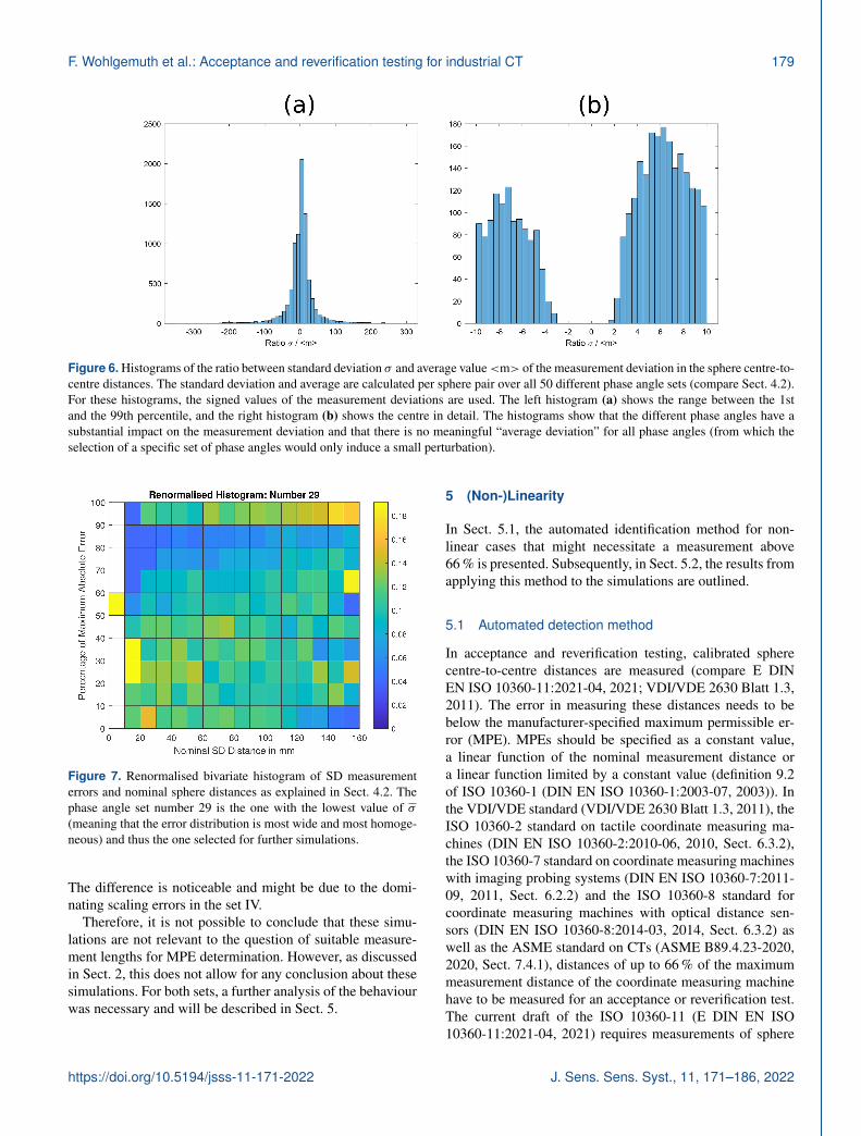
for the ratio of nominal distances in this nominal dis-tance bin width that produced an SD error within thisSD error bin. The more homogeneous this number isacross the bins, the more homogeneous the distributionis. An example for the resulting histogram is shown inFig. 7.

5. In each nominal distance bin, the standard deviation ofthe ratios in the different SD error bins was calculated.Then, the arithmetic mean value σ of all these standarddeviations was calculated.

The phase angle simulation with the lowest value of σ isthe simulation that produces the most homogeneous and widedistribution of SD errors across all nominal distances. Thus,it is the most relevant phase angle set for this investigationand was used furthermore for the subsequent simulations.

The simulation with dynamic misalignments using the se-lected phase angles and the initial misalignment amplitudesestimated in Sect. 3.1 has a maximum SD error of above100 µm. As in Sect. 4.1, we again wanted to decrease mis-alignment amplitudes such as to reach a maximum SD errorbetween 10–20 µm. Therefore, we reduced all dynamic mis-alignment amplitudes in steps of 10 % of their initial value.At 20 % of the initial value, a maximum SD error of 18.3 µmwas reached. We repeated the simulations with negative mis-alignment amplitudes and obtained approximately the sameresult (maximum SD error of 18.8 µm at 20 %).

4.3 Simulations with combined misalignments

We performed two sets of simulations with all static and alldynamic misalignments (with the phase angle set selected inSect. 4.2) combined. In the first set of simulations (IV fromTable 1), we used the misalignment amplitudes that we hadinitially estimated (in Sect. 3.1). We think that these simula-tions represent a CT system which has quickly been alignedand is “low-effort”. As a second set of simulations (V fromTable 1), for each misalignment, the chosen amplitudes thatproduce errors within 10–20 µm were used. This set of pa-rameters represents a CT system in which dominant geo-metrical error sources have been characterised and mitigated.Therefore, it represents a “medium-effort” CT system.

For both parameter sets, the initial misalignment ampli-tudes in their combination produced unrealistically high SDerrors (or, in the case of set IV, simulations resulting in vol-umes as seen in Fig. 5). Consequently, all misalignment am-plitudes were reduced by multiplication with a common fac-tor. For the low-effort CT system set IV, the factors ±0.2,±0.15, . . . ,±0.05 were simulated. For the medium-effort CTsystem set V, the factors±1,±0.8, . . . ,±0.2 were simulated.

In all simulations with combined misalignments, there isno linearity of the SD errors with respect to the nominalsphere distance. For set IV, all correlation coefficients are be-low 0.8. For set V, all correlation coefficients are below 0.5.



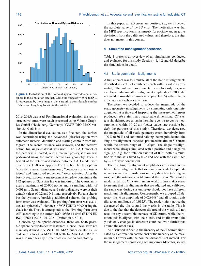
Figure 6. Histograms of the ratio between standard deviation σ and average value<m> of the measurement deviation in the sphere centre-to-centre distances. The standard deviation and average are calculated per sphere pair over all 50 different phase angle sets (compare Sect. 4.2).For these histograms, the signed values of the measurement deviations are used. The left histogram (a) shows the range between the 1stand the 99th percentile, and the right histogram (b) shows the centre in detail. The histograms show that the different phase angles have asubstantial impact on the measurement deviation and that there is no meaningful “average deviation” for all phase angles (from which theselection of a specific set of phase angles would only induce a small perturbation).

Figure 7. Renormalised bivariate histogram of SD measurementerrors and nominal sphere distances as explained in Sect. 4.2. Thephase angle set number 29 is the one with the lowest value of σ(meaning that the error distribution is most wide and most homoge-neous) and thus the one selected for further simulations.

The difference is noticeable and might be due to the domi-nating scaling errors in the set IV.

Therefore, it is not possible to conclude that these simu-lations are not relevant to the question of suitable measure-ment lengths for MPE determination. However, as discussedin Sect. 2, this does not allow for any conclusion about thesesimulations. For both sets, a further analysis of the behaviourwas necessary and will be described in Sect. 5.

5 (Non-)Linearity

In Sect. 5.1, the automated identification method for non-linear cases that might necessitate a measurement above66 % is presented. Subsequently, in Sect. 5.2, the results fromapplying this method to the simulations are outlined.

5.1 Automated detection method

In acceptance and reverification testing, calibrated spherecentre-to-centre distances are measured (compare E DINEN ISO 10360-11:2021-04, 2021; VDI/VDE 2630 Blatt 1.3,2011). The error in measuring these distances needs to bebelow the manufacturer-specified maximum permissible er-ror (MPE). MPEs should be specified as a constant value,a linear function of the nominal measurement distance ora linear function limited by a constant value (definition 9.2of ISO 10360-1 (DIN EN ISO 10360-1:2003-07, 2003)). Inthe VDI/VDE standard (VDI/VDE 2630 Blatt 1.3, 2011), theISO 10360-2 standard on tactile coordinate measuring ma-chines (DIN EN ISO 10360-2:2010-06, 2010, Sect. 6.3.2),the ISO 10360-7 standard on coordinate measuring machineswith imaging probing systems (DIN EN ISO 10360-7:2011-09, 2011, Sect. 6.2.2) and the ISO 10360-8 standard forcoordinate measuring machines with optical distance sen-sors (DIN EN ISO 10360-8:2014-03, 2014, Sect. 6.3.2) aswell as the ASME standard on CTs (ASME B89.4.23-2020,2020, Sect. 7.4.1), distances of up to 66 % of the maximummeasurement distance of the coordinate measuring machinehave to be measured for an acceptance or reverification test.The current draft of the ISO 10360-11 (E DIN EN ISO10360-11:2021-04, 2021) requires measurements of sphere



Figure 8. A scenario in which the convex hulls of the measurementpoints below 66 % and of all measurement points (including above66 %) agree up until 66 %. We assume that an MPE specification ac-cording to Eq. (3) based on the points below 66 % would encompassthe points above 66 % as well.

distances of up to 85 %. This requirement makes sense ifthere are effects between 66 % and 85 % of the maximummeasurement distance that necessitate a different MPE spec-ification than below. In light of the form of the MPE specifi-cation, these effects would need to be non-linear in the mea-surement length. The MPE specification should follow theform given by Eq. (3).

MPE= A+L/K (3)

Here, the manufacturer can choose A and K freely. Theextreme choices are obviously A= 0 (minimising K) orK→∞ (maximising A). Any effect necessitating measure-ments of up to 85 % would therefore mean that the manufac-turer would need to change their choice of A and K becauseof the additional data above 66 %. The choice of the valuesfor A andK is (and ought to be) at the discretion of the man-ufacturer – therefore, no clear criterion can be derived fromthe standard. We however propose to inspect the convex hull(see O’Rourke, 1998) of the point set of nominal measure-ment distances and respective measurement deviations. If theconvex hull below 66 % stays constant no matter whether allpoints or only the points up to 66 % are used, there is no rea-son for a requirement to measure lengths longer than 66 %,and this simulated case is deemed not relevant for the MPEquestion. If however, the convex hull does change, this sim-ulated case should be inspected as it might be relevant. Theapproach is illustrated in Figs. 8 and 9.

In contrast to Figs. 8 and 9, we truncate the bottom partof the convex hull, using only parts with positive slope. Fur-ther, we do not consider any decreases in the slope of the66 % convex hull that happen in the regime between 60 %and 66 % as relevant as these can be boundary effects, and

Figure 9. A scenario in which the convex hulls of the measurementpoints below 66 % and of all measurement points (including above66 %) do not agree below 66 %. There are points above 66 % whoseincrease in measurement deviation is stronger than linear, and thuswe think that in this case, an MPE specification for both point sets(up until 66 % and all points) could reasonably be different. A MPEspecification for below 66 % might not hold for the points above.Such an extreme scenario as depicted here could not be observed inany simulation of this study.

we do not believe a manufacturer would readjust their MPEspecification based on these.

The convex hull criterion as presented here is a worst-casescenario as there is no safety distance to the measured points,and the last (and therefore lowest) slope of the 66 % convexhull is used for comparison. The choice of a higher slope islegitimate and is an added safety margin for the manufac-turer. Further, accounting for the test value uncertainty, anymanufacturer will keep a certain distance to all measurementpoints when constructing an MPE. We therefore think thatin a real MPE specification scenario, the MPE will be cho-sen with more of a safety margin. The convex hull criteriondoes however allow for the automatic identification of caseswhich are definitely not relevant for the question of maxi-mum length (i.e., those for which the convex hulls agree).The cases in which the convex hulls do not agree need visualinspection – the criterion does not allow for an automated de-cision that, based on this data set, a measurement of lengthslonger than 66 % is necessary. This is again due to the flexi-bility in the MPE statement and the resulting need for a visualinspection.

To quantify the difference between both convex hulls (ifthere is any), we extend the last clockwise part of the convexhull with a positive slope into a linear function (representinga “convex-hull-derived” MPE specification). If both convexhulls differ below 66 % (as in the Fig. 9), there needs to beat least one data point above the extended linear function de-rived from the 66 % convex hull. To quantify the difference,



we use the maximum distance of all these data points fromthis extended linear function. The distance is measured in thedirection of the “measurement deviation” axis only. Return-ing to the argument of a reasonable MPE specification by amanufacturer, we quantify this distance as a percentage ofthe observed measurement deviation at this data point. Themotivation is that a manufacturer will choose a safety dis-tance; thus exceeding this worst-case MPE statement by afew percent is not relevant.

5.2 Results

Out of a total of 164 simulations from Sect. 4.1 and 4.2(single static misalignments and isolated dynamic misalign-ments), only seven show a maximum difference that is morethan 5 % of the measured SD error. Two of these are tiltsof the rotation axis around the x axis (axis perpendicular tobeam and rotation axis; see Fig. 2) by −0.0125 and −0.025◦

(see Fig. 10). The data points in those plots follow a roughlylinear trend, and, thus, we expect a human to specify a MPEfollowing this general linear trend. The other five are dy-namic simulations with random phase angles from Sect. 4.2(see Fig. 11 and the first plot of Fig. 12).

For the simulations with the combined errors (Sect. 4.3),we performed the same analysis. For the initial misalignmentestimate simulations (set IV, eight simulations), no simula-tion shows a difference above 5 %. For the simulations withadapted misalignment amplitudes (set V, 10 simulations),three simulations show a difference above 5 % (see Fig. 12).This finding agrees with the increase in correlation coeffi-cient ρ (compare Sect. 4.3) and the hypothesis of dominatingscaling errors for set IV as scaling errors are strictly linear inthe measurement length.

Summarising, from 182 simulations, only 10 are identifiedas possibly relevant by the convex hull criterion due to a dif-ference of more than 5 % between both convex hulls. As dis-cussed above, this does not necessarily mean that they wouldactually fail a manufacturer’s MPE specification above 66 %due to the freedom in specifying the MPE. Of these 10 cases,two (the rotation axis displacement) have a general lineartrend that would probably lead to an MPE with a higher slopein specification (these can visually be classified as “roughlylinear” in the sense of Fig. 1). The other eight cases are fivesets of random phase angles for the dynamic errors (Figs. 11and 12) and three simulations with combined misalignmentswith rescaled amplitudes (set V; see Fig. 12). These caseswill be discussed again in Sect. 6.

6 Probing form errors

As described in Sect. 3.3, probing form errors were also eval-uated. Besides sphere distances, probing form errors are an-other important characteristic in acceptance testing (E DINEN ISO 10360-11:2021-04, 2021; VDI/VDE 2630 Blatt 1.3,2011). A complete specification is required to cover at least

probing errors (probing form errors and probing size er-rors) and the sphere distance errors (Table 3 in E DIN ENISO 10360-11:2021-04, 2021). Therefore, these characteris-tics should be seen as a set of indicators about CT systemperformance. It is not necessary that all characteristics de-tect all possible error sources. We therefore analyse the im-pact of the geometrical misalignments simulated thus far onthe probing form errors. The rationale behind this is that theeight cases needing a visual – and thus necessarily subjec-tive – analysis in Sect. 5 do not need to be analysed further ifthe probing form error is very sensitive to them. In the lattercase, the probing form error will detect the underlying geo-metrical misalignment sufficiently, and therefore, even if themisalignments are not completely accounted for in the MPEstatement (“not completely accounted for” should be read as“underestimated by a few percent”), there is no risk that themisalignment is not detected during acceptance or reverifica-tion testing.

Within this section, we analyse the sphere-wise increase inform error in a simulation with misalignment in comparisonto a simulation without misalignment. Further, we report themaximum increase in form error over all spheres.

For the 50 random phase angle simulations with the dy-namic misalignments (set II), the probing form error increaseis above 100 µm for all phases and above 200 µm for most.We claim that these values will not be acceptable to a cus-tomer and that therefore, the potential that – for 10 % of thesesimulations – the MPE specification for sphere distance er-rors might be too low based on data points up to 66 % (com-pare Figs. 11 and 12) is not crucial as another part of theacceptance test will more reliably detect the underlying mis-alignment.

For the set of combined misalignments based on therescaled simulations (set V), all probing form error increasesare above 270 µm. Therefore, the misalignments can well bedetected using the probing form error test, and the potentialthat, for some of these simulations, the MPE specificationfor the sphere distance errors might be too low based on thedata up to 66 % (compare Fig. 12) can again be neglected asthe probing form error part of the acceptance test will easilydetect the geometrical misalignments.

For the set of combined initial estimate misalignments (setIV), the probing form errors are above 300 µm for factorswith magnitude greater or equal to 0.1. For the factor ±0.05,the probing form errors are at approximately 32 µm. This isstill a noticeable probing form error, but it is much more real-istic. With set IV, we did not identify any potentially relevantcases in Sect. 5. This simulation shows that different parts ofthe acceptance test are sensitive to different misalignments.Both the lowest factors of set IV and set V lead to compara-ble SD errors, but their probing form error differs by an orderof magnitude. The scaling errors that are dominant in set IVthus seem to have a much lower impact on the probing formerrors (see discussion below).



Figure 10. Convex hull analysis of non-linearity for the rotation axis tilt around the x axis (axis perpendicular to beam and rotation axis;see Fig. 2) by −0.0125 and −0.025◦. The plots show the data points, both convex hulls (using points until 66 % and using all points) as wellas derived MPE specifications. The 1abs marks the data point with the largest distance to the 66 % MPE specification. The simulations arepart of simulation set I. We are convinced that a human would visually not specify such a low slope for the below 66 % MPE specification asthe automated algorithm used in this study. In this sense, the criterion employed here is, as discussed in the text, a worst-case criterion. Wewould expect most MPEs specified based on this picture to follow the general linear trend of the data points.

The static geometry misalignments (simulation set I) merita more in-depth discussion:

– Detector position perpendicular to beam axis (x and yaxis). For the detector translations perpendicular to thebeam axis, probing form errors are very high (all above100 µm). Probing form errors seem very sensitive to thismisalignment.

– Detector position along beam axis (z axis). Only fora high misalignment of 3.75 mm or −3.75 mm are theprobing form errors above 10 µm (10.5 µm or 15.2 µm).For all smaller misalignments, the probing form errorsare below 8 µm. The probing form errors are thereforenot very suitable to detect this misalignment that causesstrong scaling errors.

– Detector orientation. For the detector tilt around the xand y axis, the probing form errors are below 5 µm –probing form errors are not very sensitive to these mis-alignments. For the tilt around the z axis, the probingform errors are higher and reach approximately 17 µmfor a 0.057296◦ tilt.

– Source position. For the translation along the x axis, theprobing form errors are high (all above 340 µm). Alongthe y axis, the probing form errors are considerablysmaller, with approx. 18 µm at the setting producing SDerrors within 10–20 µm. The scaling error (z axis trans-lation) induces small probing form errors below 9 µm.For the z axis translation of the source that leads to SDerrors within 10–20 µm, the probing form errors are be-low 2 µm. Therefore, also for this scaling error, probing

form errors are again not very suitable for detecting thegeometrical misalignment.

– Rotation axis tilt. A rotation axis tilt around the z axisby ±0.05◦ (leading to SD errors within 10–20 µm) pro-duces probing form errors of 17 µm or 18 µm. The ro-tation axis tilt around the x axis results in small prob-ing form errors below 7 µm for absolute misalignmentamplitudes of± 0.025◦ and below. Unlike with scalingerrors, the increase of probing form errors with increas-ing misalignment amplitude is stronger (15 µm or 14 µmat± 0.05◦ and 31 µm at ±0.1◦), but the amplitude thatresults in SD errors within 10–20 µm does not result inequally high or higher probing form errors.

– Rotation axis position. For translations along the beamdirection (z axis), probing form errors are below 8 µm.At the magnitude that leads to SD errors within 10–20 µm, the form errors are below 2 µm. Again, the scal-ing error does not impact form errors strongly.

Summarising, dynamic misalignments of the rotation axisand the rotary table can be detected very well by inspect-ing probing form errors, while scaling misalignments leadto negligible probing form errors. Other static misalignmentsshow a more complex dependence – with some resulting inlarge probing form errors, while others have less of an im-pact. The simulation study clearly shows the need for includ-ing both probing form errors and sphere distance measure-ments in acceptance testing as both are sensitive to differentgeometrical misalignments.



Figure 11. Convex hull analysis of non-linearity: the plots show the data points, both convex hulls (using points until 66 % and using allpoints) as well as derived MPE specifications. The 1abs marks the data point with the largest distance to the 66 % MPE specification. Theplots are for four of the five simulations with random phase angles from Sect. 4.3 and part of simulation set II (for the last one, see Fig. 12).

The eight cases mentioned at the end of Sect. 5.2 as casesin which the data points for SD errors above 66 % might ne-cessitate a different choice for the MPE are all cases in whichprobing form errors are very pronounced and furthermorecases in which misalignments that are very well captured byprobing form errors cause the SD errors. We therefore thinkthat these cases are negligible for acceptance testing seen asa whole, as the probing form error will detect the underlyingmisalignments reliably, and that these eight cases are thus noreason for a requirement to measure lengths above 66 % forthe SD errors.

7 Conclusions

We performed a simulative study to investigate sphere dis-tance and form measurements that are typically used inacceptance and reverification testing (see, for example, EDIN EN ISO 10360-11:2021-04, 2021; VDI/VDE 2630 Blatt1.3, 2011). For this purpose, we designed a virtual simu-lation artefact and estimated several geometrical misalign-ments. Our initial estimates of the geometrical misalign-ments mostly produced unrealistically high measurement er-rors for the sphere distances. We therefore needed to re-duce our initial estimates. We discussed the problem of find-ing a suitable automated identification for whether a simu-lation would indicate a need for deviating from the estab-



Figure 12. Convex hull analysis of non-linearity: the plots show the data points, both convex hulls (using points until 66 % and using allpoints) as well as derived MPE specifications. The 1abs marks the data point with the largest distance to the 66 % MPE specification. Theplot (a) is the last one for the simulations for the five random phase angles from Sect. 4.3 and part of simulation set II (for the first four, seeFig. 11). The other three plots (b), (c) and (d) are for simulation set V (see Sect. 4.3).

lished 66 % measurement rule for sphere distances (as in-cluded in DIN EN ISO 10360-2:2010-06, 2010; DIN ENISO 10360-7:2011-09, 2011; DIN EN ISO 10360-8:2014-03, 2014; VDI/VDE 2630 Blatt 1.3, 2011). We presented aworst-case criterion based on constructing the convex hull ofthe data points collected and used this to evaluate our sim-ulations. Of a total of 182 simulations, only 10 were iden-tified based on this worst-case criterion. Two of these weregauged as having a linear trend and thus being a shortcomingof the criterion. The other eight are due to simulations withdynamic rotary table misalignments. In general, the test pro-cedure in acceptance and reverification testing should charac-terise CT system performance and thus also detect any geo-

metrical misalignments. It is therefore important that at leastone of the mandatory characteristics (probing error (formor size) or sphere distance error) of the standardised test isable to detect each geometrical misalignment. It is howevernot necessary that each characteristic does so or that eachcharacteristic does so with a high sensitivity. We thereforealso inspected the impact of geometrical misalignments onthe probing form errors. This analysis showed that the mis-alignments that produce the smallest probing form errors arethe scaling misalignments that produce sphere distance er-rors linear in the nominal measurement distance. All othermisalignments can – to some extent – be detected by probingform errors as well.



Even for most geometrical misalignments that are welldetected by probing form errors, there is, according to ourworst-case convex hull criterion, no behaviour that would ne-cessitate a deviation from the established 66 % requirement.The dynamic rotary table misalignments result in especiallypronounced probing form errors. In the eight cases in whichdynamic rotary table misalignments are present and the con-vex hull criterion indicates a possibility for a need to mea-sure longer lengths, the underlying misalignments can there-fore be well identified by inspecting the probing form error.An extension of the measurement lengths for the SD errorto capture these misalignments even better with the SD erroras well would constitute unnecessary additional effort as theprobing form error is clearly more sensitive.

Overall, the highest deviations from the conservative MPEestimate derived based on the convex hull are 8 % of the mea-sured SD error – we think that considering test value uncer-tainty, manufacturer safety margin and freedom of choice inthe MPE specification, the MPE specification will rarely bebelow this error. Should it happen, both user and manufac-turer still have a clear indication for the underlying geometri-cal misalignment from high probing form errors. Besides theroughly linear behaviour of the rotation axis tilt around thex axis which was found by our automated convex hull cri-terion but which we visually discarded, there is no scenarioin which, due to more than linear behaviour, a geometricalmisalignment can not be detected neither with the SD mea-surements up to 66 %, nor with the form measurements. Asboth are mandatory, no user or manufacturer can perform anacceptance test without detecting the geometrical misalign-ments studied in this work.

Based on the simulation study presented here, there isno technical reason for measuring SD errors with nominallengths above the established 66 % of the maximum lengthfrom other comparable standards (DIN EN ISO 10360-2:2010-06, 2010; DIN EN ISO 10360-7:2011-09, 2011; DINEN ISO 10360-8:2014-03, 2014; VDI/VDE 2630 Blatt 1.3,2011).

Code availability. The code is not publicly accessible but can berequested from the corresponding author if required.

Data availability. Due to the size (more than 6 TB), the simulationdata are not publicly available and can be requested from the authorsif needed.

Author contributions. The author contributions are declared ac-cording to CASRAI CRediT. KDI, WK, IS, TH and FW were in-volved in conceptualisation and methodology. FW was responsiblefor data curation, formal analysis, investigation, project administra-tion, software, visualisation and writing – original draft. KDI, WK,IS and TH were responsible for supervision and writing – reviewand editing.

Competing interests. Werth Messtechnik GmbH and Carl ZeissIndustrielle Messtechnik GmbH are manufacturers of industrialcomputed tomography systems. This study received funding fromthese companies.

Disclaimer. Publisher’s note: Copernicus Publications remainsneutral with regard to jurisdictional claims in published maps andinstitutional affiliations.

Acknowledgements. We want to thank Werth MesstechnikGmbH and Carl Zeiss Industrielle Messtechnik GmbH for the finan-cial support of the project as well as Volume Graphics GmbH (Hei-delberg, Germany) for the kind permission to use their VGSTUDIOMAX evaluation software.

Financial support. This study received funding from WerthMesstechnik GmbH and Carl Zeiss Industrielle MesstechnikGmbH.

Review statement. This paper was edited by Thomas Fröhlichand reviewed by two anonymous referees.

References

ASME B89.4.23-2020: X-Ray Computed Tomography (CT) Per-formance Evaluation, ISBN 9780791873830, 2020.

Bellon, C., Deresch, A., Gollwitzer, C., and Jaenisch, G.-R.: Ra-diographic Simulator aRTist: Version 2, in: 18th World Con-ference on Nondestructive Testing, 16–20 April 2012, Durban,South Africa, http://www.ndt.net/?id=12664 (last access: 10 June2022), 2012.

Carmignato, S., Dewulf, W., and Leach, R. (Eds.): Industrial X-RayComputed Tomography, 1st edn., Springer International Pub-lishing, ISBN 978-3-319-59573-3, https://doi.org/10.1007/978-3-319-59573-3, 2018.

DIN EN ISO 10360-1:2003-07: Annahmeprüfung und Bestä-tigungsprüfung für Koordinatenmessgeräte (KMG) Teil1: Begriffe (enthält Berichtigung AC:2002) (ISO 10360-1:2000+Cor.1:2002), 2003.

DIN EN ISO 10360-2:2010-06: Geometrische Produktspezifikation(GPS) – Annahmeprüfung und Bestätigungsprüfung für Koordi-natenmessgeräte (KMG) – Teil 2: KMG angewendet für Längen-messungen (ISO 10360-2:2009), 2010.

DIN EN ISO 10360-3:2000-08: Geometrische Produktspezifika-tion (GPS) Annahmeprüfung und Bestätigungsprüfung für Ko-ordinatenmessgeräte (KMG) Teil 3: KMG mit der Achse einesDrehtisches als vierte Achse (ISO 10360-3:2000), 2000.

DIN EN ISO 10360-7:2011-09: Geometrische Produktspezifikation(GPS) – Annahme- und Bestätigungsprüfung für Koordinaten-messgeräte (KMG) – Teil 7: KMG mit Bildverarbeitungssyste-men (ISO 10360-7:2011), 2011.

DIN EN ISO 10360-8:2014-03: Geometrische Produktspezifikationund -prüfung (GPS) – Annahme- und Bestätigungsprüfung für


http://www.ndt.net/?id=12664

https://doi.org/10.1007/978-3-319-59573-3

https://doi.org/10.1007/978-3-319-59573-3


Koordinatenmesssysteme (KMS) – Teil 8: KMG mit optischenAbstandssensoren (ISO 10360-8:2013), 2014.

E DIN EN ISO 10360-11:2021-04: Geometrische Produktspez-ifikation und -prüfung (GPS) – Annahmeprüfung und Bestä-tigungsprüfung für Koordinatenmessgeräte (KMG) – Teil 11:Computertomografie (ISO/DIS 10360-11:2021), 2021.

Fahrmeir, L., Kneib, T., and Lang, S.: Regression, 2ndedn., Springer Berlin Heidelberg, ISBN 978-3-642-01837-4,https://doi.org/10.1007/978-3-642-01837-4, 2009.

Jaganmohan, P., Muralikrishnan, B., Shilling, M., and Morse, E. P.:Trends in Geometric Error of X-ray Computed Tomography In-struments Observed at Different Locations in the MeasurementVolume, in: ASPE 2020 Annual Meeting Volume 73, 122–127,ISBN 978-1-7138-2046-8, 2020.

Muralikrishnan, B., Shilling, M., Phillips, S., Ren, W., Lee,V., and Kim, F.: X-ray Computed Tomography Instru-ment Performance Evaluation, Part I: Sensitivity to Detec-tor Geometry Errors, J. Res. Natl. Inst. Stan., 124, 124014,https://doi.org/10.6028/jres.124.014, 2019a.

Muralikrishnan, B., Shilling, M., Phillips, S., Ren, W., Lee,V., and Kim, F.: X-ray Computed Tomography Instru-ment Performance Evaluation, Part II: Sensitivity to Rota-tion Stage Errors, J. Res. Natl. Inst. Stan., 124, 124015,https://doi.org/10.6028/jres.124.015, 2019b.

Muralikrishnan, B., Shilling, M., Phillips, S., Ren, W., Lee, V., Kim,F., Alberts, G., and Aloisi, V.: X-ray computed tomography in-strument performance evaluation: Detecting geometry errors us-ing a calibrated artifact, in: Dimensional Optical Metrology andInspection for Practical Applications VIII, edited by: Zhang, S.and Harding, K. G., SPIE, https://doi.org/10.1117/12.2518108,2019c.

O’Rourke, J.: Computational Geometry in C, 2nd edn.,Cambridge University Press, ISBN 9780511804120,https://doi.org/10.1017/cbo9780511804120, 1998.

van Aarle, W., Palenstijn, W. J., Beenhouwer, J. D., Altantzis,T., Bals, S., Batenburg, K. J., and Sijbers, J.: The AS-TRA Toolbox: A platform for advanced algorithm develop-ment in electron tomography, Ultramicroscopy, 157, 35–47,https://doi.org/10.1016/j.ultramic.2015.05.002, 2015.

van Aarle, W., Palenstijn, W. J., Cant, J., Janssens, E., Ble-ichrodt, F., Dabravolski, A., Beenhouwer, J. D., Batenburg,K. J., and Sijbers, J.: Fast and flexible X-ray tomographyusing the ASTRA toolbox, Opt. Express, 24, 25129–25147,https://doi.org/10.1364/oe.24.025129, 2016.

VDI/VDE 2617 Blatt 4: Leitfaden zur Anwendung von DINEN ISO 10360-3 für Koordinatenmessgeräte mit zusätzlichenDrehachsen, May 2006.

VDI/VDE 2630 Blatt 1.3: Leitfaden zur Anwendung von DIN ENISO 10360 für Koordinatenmessgeräte mit CT-Sensoren, Decem-ber 2011.

Wohlgemuth, F., Müller, A., and Hausotte, T.: Development of avirtual metrological CT for numerical measurement uncertaintydetermination using aRTist 2, tm – Technisches Messen, 85, 728–737, https://doi.org/10.1515/teme-2018-0044, 2018.

Wohlgemuth, F., Wolter, F., and Hausotte, T.: Digitale Zwill-inge metrologischer Röntgencomputertomografen für die nu-merische Messunsicherheitsbestimmung, in: ZfP heute. Wis-senschaftliche Beiträge zur zerstörungsfreien Prüfung 2020,edited by: Deutsche Gesellschaft für Zerstörungsfreie Prüfunge.V., pp. 106–110, ISBN 978-3-947971-10-7, https://www.ndt.net/?id=25501 (last access: 10 June 2022), 2020.


https://doi.org/10.1007/978-3-642-01837-4

https://doi.org/10.6028/jres.124.014

https://doi.org/10.6028/jres.124.015

https://doi.org/10.1117/12.2518108

https://doi.org/10.1017/cbo9780511804120

https://doi.org/10.1016/j.ultramic.2015.05.002

https://doi.org/10.1364/oe.24.025129

https://doi.org/10.1515/teme-2018-0044

https://www.ndt.net/?id=25501

https://www.ndt.net/?id=25501

a simulative study on geometrical misalignments - JSSS

Documents

Transcript of a simulative study on geometrical misalignments - JSSS