The Mathematics of Geometrical and Physical Optics The k-function and its Ramifications
224
Orestes N. Stavroudis The Mathematics of Geometrical and Physical Optics The k-function and its Ramifications
Transcript of The Mathematics of Geometrical and Physical Optics The k-function and its Ramifications
Orestes N. Stavroudis
The Mathematics of Geometrical andPhysical Optics
The k-function and its Ramifications

The AuthorProf. Dr. Orestes N. StavroudisCentro de Investigaciones en Optica,Leon, Guanajuato, [email protected]
Cover picturePersistence of Vision Raytracer Version 3.5Sample FileAuthor: Christopher J. Huff
All books published by Wiley-VCH are carefullyproduced. Nevertheless, authors, editors, and publisherdo not warrant the information contained in thesebooks, including this book, to be free of errors. Readersare advised to keep in mind that statements, data,illustrations, procedural details or other items mayinadvertently be inaccurate.
Library of Congress Card No.:applied for
British Library Cataloguing-in-Publication DataA catalogue record for this book is available from theBritish Library.
Bibliographic information published byDie Deutsche BibliothekDie Deutsche Bibliothek lists this publication in theDeutsche Nationalbibliografie; detailed bibliographicdata is available in the Internet at <http://dnb.ddb.de>.
c© 2006 WILEY-VCH Verlag GmbH & Co. KGaA,Weinheim
All rights reserved (including those of translation intoother languages). No part of this book may bereproduced in any form – by photoprinting, microfilm,or any other means – nor transmitted or translated into amachine language without written permission from thepublishers. Registered names, trademarks, etc. used inthis book, even when not specifically marked as such,are not to be considered unprotected by law.
Printed in the Federal Republic of Germany
Typesetting Steingraeber Satztechnik GmbH,Ladenburg
Printing Strauss GmbH, Morlenbach
Binding Schaffer GmbH, Grunstadt
ISBN-13: 978-3-527-40448-3ISBN-10: 3-527-40448-1
Acknowledgements
Many hands make the work light. It is my pleasure to acknowledge and thank those whoseefforts made this work possible. These are (in alphabetic order): Maximiliano Avendano-Alejo, Isidro Cornejo, Lark London, Christopher Stavroudis, Dorle Stavroudis, and manyformer students whose helpful comments and snide remarks were of immensurable value.Thanks are also due to my project editor, Ulrike Werner, who skillfully and tactfully, led mein the proper direction.

The Mathematics of Geometrical and Physical Optics: The k-function and its Ramifications. O.N. StavroudisCopyright c© 2006 WILEY-VCH Verlag GmbH & Co. KGaA, WeinheimISBN: 3-527-40448-1
Contents
I Preliminaries 1
1 Fermat’s Principle and the Variational Calculus 31.1 Rays in Inhomogeneous Media . . . . . . . . . . . . . . . . . . . . . . . . 41.2 The Calculus of Variations . . . . . . . . . . . . . . . . . . . . . . . . . . 51.3 The Parametric Representation . . . . . . . . . . . . . . . . . . . . . . . . 71.4 The Vector Notation . . . . . . . . . . . . . . . . . . . . . . . . . . . . . . 91.5 The Inhomogeneous Optical Medium . . . . . . . . . . . . . . . . . . . . 101.6 The Maxwell Fish Eye . . . . . . . . . . . . . . . . . . . . . . . . . . . . 111.7 The Homogeneous Medium . . . . . . . . . . . . . . . . . . . . . . . . . 111.8 Anisotropic Media . . . . . . . . . . . . . . . . . . . . . . . . . . . . . . 12
2 Space Curves and Ray Paths 152.1 Space Curves . . . . . . . . . . . . . . . . . . . . . . . . . . . . . . . . . 152.2 The Vector Trihedron . . . . . . . . . . . . . . . . . . . . . . . . . . . . . 162.3 The Frenet-Serret Equations . . . . . . . . . . . . . . . . . . . . . . . . . 182.4 When the Parameter is Arbitrary . . . . . . . . . . . . . . . . . . . . . . . 192.5 The Directional Derivative . . . . . . . . . . . . . . . . . . . . . . . . . . 202.6 The Cylindrical Helix . . . . . . . . . . . . . . . . . . . . . . . . . . . . . 212.7 The Conic Section . . . . . . . . . . . . . . . . . . . . . . . . . . . . . . . 222.8 The Ray Equation . . . . . . . . . . . . . . . . . . . . . . . . . . . . . . . 252.9 More on the Fish Eye . . . . . . . . . . . . . . . . . . . . . . . . . . . . . 26
3 The Hilbert Integral and the Hamilton-Jacobi Theory 293.1 A Digression on the Gradient . . . . . . . . . . . . . . . . . . . . . . . . . 323.2 The Hilbert Integral. Parametric Case . . . . . . . . . . . . . . . . . . . . 333.3 Application to Geometrical Optics . . . . . . . . . . . . . . . . . . . . . . 343.4 The Condition for Transversality . . . . . . . . . . . . . . . . . . . . . . . 343.5 The Total Differential Equation . . . . . . . . . . . . . . . . . . . . . . . . 353.6 More on the Helix . . . . . . . . . . . . . . . . . . . . . . . . . . . . . . . 373.7 Snell’s Law . . . . . . . . . . . . . . . . . . . . . . . . . . . . . . . . . . 393.8 The Hamilton-Jacobi Partial Differential Equations . . . . . . . . . . . . . 413.9 The Eikonal Equation . . . . . . . . . . . . . . . . . . . . . . . . . . . . . 43
4 The Differential Geometry of Surfaces 454.1 Parametric Curves . . . . . . . . . . . . . . . . . . . . . . . . . . . . . . . 454.2 Surface Normals . . . . . . . . . . . . . . . . . . . . . . . . . . . . . . . 454.3 The Theorem of Meusnier . . . . . . . . . . . . . . . . . . . . . . . . . . 474.4 The Theorem of Gauss . . . . . . . . . . . . . . . . . . . . . . . . . . . . 494.5 Geodesics on a Surface . . . . . . . . . . . . . . . . . . . . . . . . . . . . 514.6 The Weingarten Equations . . . . . . . . . . . . . . . . . . . . . . . . . . 534.7 Transformation of Parameters . . . . . . . . . . . . . . . . . . . . . . . . . 55
XII Contents
4.8 When the Parametric Curves are Conjugates . . . . . . . . . . . . . . . . . 574.9 When F �= 0 . . . . . . . . . . . . . . . . . . . . . . . . . . . . . . . . . 604.10 The Structure of the Prolate Spheroid . . . . . . . . . . . . . . . . . . . . 614.11 Other Ways of Representing Surfaces . . . . . . . . . . . . . . . . . . . . 64
5 Partial Differential Equations of the First Order 675.1 The Linear Equation. The Method of Characteristics . . . . . . . . . . . . 685.2 The Homogeneous Function . . . . . . . . . . . . . . . . . . . . . . . . . 705.3 The Bilinear Concomitant . . . . . . . . . . . . . . . . . . . . . . . . . . . 715.4 Non-Linear Equation: The Method of Lagrange and Charpit . . . . . . . . 725.5 The General Solution . . . . . . . . . . . . . . . . . . . . . . . . . . . . . 735.6 The Extension to Three Independent Variables . . . . . . . . . . . . . . . . 765.7 The Eikonal Equation. The Complete Integral . . . . . . . . . . . . . . . . 775.8 The Eikonal Equation. The General Solution . . . . . . . . . . . . . . . . 795.9 The Eikonal Equation. Proof of the Pudding . . . . . . . . . . . . . . . . . 81
II The k-function 83
6 The Geometry of Wave Fronts 856.1 Preliminary Calculations . . . . . . . . . . . . . . . . . . . . . . . . . . . 856.2 The Caustic Surface . . . . . . . . . . . . . . . . . . . . . . . . . . . . . . 896.3 Special Surfaces I: Plane and Spherical Wavefronts . . . . . . . . . . . . . 906.4 Parameter Transformations . . . . . . . . . . . . . . . . . . . . . . . . . . 926.5 Asymptotic Curves and Isotropic Directions . . . . . . . . . . . . . . . . . 94
7 Ray Tracing: Generalized and Otherwise 977.1 The Transfer Equations . . . . . . . . . . . . . . . . . . . . . . . . . . . . 987.2 The Ancillary Quantities . . . . . . . . . . . . . . . . . . . . . . . . . . . 1007.3 The Refraction Equations . . . . . . . . . . . . . . . . . . . . . . . . . . . 1007.4 Rotational Symmetry . . . . . . . . . . . . . . . . . . . . . . . . . . . . . 1027.5 The Paraxial Approximation . . . . . . . . . . . . . . . . . . . . . . . . . 1037.6 Generalized Ray Tracing – Transfer . . . . . . . . . . . . . . . . . . . . . 1047.7 Generalized Ray Tracing – Preliminary Calculations . . . . . . . . . . . . 1057.8 Generalized Ray Tracing – Refraction . . . . . . . . . . . . . . . . . . . . 1097.9 The Caustic . . . . . . . . . . . . . . . . . . . . . . . . . . . . . . . . . . 1137.10 The Prolate Spheroid . . . . . . . . . . . . . . . . . . . . . . . . . . . . . 1137.11 Rays in the Spheroid . . . . . . . . . . . . . . . . . . . . . . . . . . . . . 114
8 Aberrations in Finite Terms 1218.1 Herzberger’s Diapoints . . . . . . . . . . . . . . . . . . . . . . . . . . . . 1228.2 Herzberger’s Fundamental Optical Invariant . . . . . . . . . . . . . . . . . 1228.3 The Lens Equation . . . . . . . . . . . . . . . . . . . . . . . . . . . . . . 1258.4 Aberrations in Finite Terms . . . . . . . . . . . . . . . . . . . . . . . . . . 1268.5 Half-Symmetric, Symmetric and Sharp Images . . . . . . . . . . . . . . . 127
Contents XIII
9 Refracting the k-Function 1319.1 Refraction . . . . . . . . . . . . . . . . . . . . . . . . . . . . . . . . . . . 1339.2 The Refracting Surface . . . . . . . . . . . . . . . . . . . . . . . . . . . . 1349.3 The Partial Derivatives . . . . . . . . . . . . . . . . . . . . . . . . . . . . 1379.4 The Finite Object Point . . . . . . . . . . . . . . . . . . . . . . . . . . . . 1409.5 The Quest for C . . . . . . . . . . . . . . . . . . . . . . . . . . . . . . . . 1429.6 Developing the Solution . . . . . . . . . . . . . . . . . . . . . . . . . . . 1449.7 Conclusions . . . . . . . . . . . . . . . . . . . . . . . . . . . . . . . . . . 146
10 Maxwell Equations and the k-Function 14710.1 The Wavefront . . . . . . . . . . . . . . . . . . . . . . . . . . . . . . . . . 14810.2 The Maxwell Equations . . . . . . . . . . . . . . . . . . . . . . . . . . . . 14810.3 Generalized Coordinates and the Nabla Operator . . . . . . . . . . . . . . 14910.4 Application to the Maxwell Equations . . . . . . . . . . . . . . . . . . . . 15010.5 Conditions on V . . . . . . . . . . . . . . . . . . . . . . . . . . . . . . . 15310.6 Conditions on the Vector V . . . . . . . . . . . . . . . . . . . . . . . . . . 15810.7 Spherical Wavefronts . . . . . . . . . . . . . . . . . . . . . . . . . . . . . 158
III Ramifications 163
11 The Modern Schiefspiegler 16511.1 Background . . . . . . . . . . . . . . . . . . . . . . . . . . . . . . . . . . 16511.2 The Single Prolate Spheroid . . . . . . . . . . . . . . . . . . . . . . . . . 16711.3 Coupled Spheroids . . . . . . . . . . . . . . . . . . . . . . . . . . . . . . 16811.4 The Condition for the Pseudo Axis . . . . . . . . . . . . . . . . . . . . . . 17211.5 Magnification and Distortion . . . . . . . . . . . . . . . . . . . . . . . . . 17511.6 Conclusion . . . . . . . . . . . . . . . . . . . . . . . . . . . . . . . . . . 177
12 The Cartesian Oval and its Kin 17912.1 The Algebraic Method . . . . . . . . . . . . . . . . . . . . . . . . . . . . 17912.2 The Object at Infinity . . . . . . . . . . . . . . . . . . . . . . . . . . . . . 18112.3 The Prolate Spheroid . . . . . . . . . . . . . . . . . . . . . . . . . . . . . 18212.4 The Hyperboloid of Two Sheets . . . . . . . . . . . . . . . . . . . . . . . 18312.5 Other Surfaces that Make Perfect Images . . . . . . . . . . . . . . . . . . . 184
13 The Pseudo Maxwell Equations 18713.1 Maxwell Equations for Inhomogeneous Media . . . . . . . . . . . . . . . . 18713.2 The Frenet-Serret Equations . . . . . . . . . . . . . . . . . . . . . . . . . 18813.3 Initial Calculations . . . . . . . . . . . . . . . . . . . . . . . . . . . . . . 18813.4 Divergence and Curl . . . . . . . . . . . . . . . . . . . . . . . . . . . . . 19013.5 Establishing the Relationship . . . . . . . . . . . . . . . . . . . . . . . . . 192
14 The Perfect Lenses of Gauss and Maxwell 19714.1 Gauss’Approach . . . . . . . . . . . . . . . . . . . . . . . . . . . . . . . 197

XIV Contents
14.2 Maxwell’s Approach . . . . . . . . . . . . . . . . . . . . . . . . . . . . . 198
A Appendix. Vector Identities 205A.1 Algebraic Identities . . . . . . . . . . . . . . . . . . . . . . . . . . . . . . 206A.2 Identities Involving First Derivatives . . . . . . . . . . . . . . . . . . . . . 207A.3 Identities Involving Second Derivatives . . . . . . . . . . . . . . . . . . . 207A.4 Gradient . . . . . . . . . . . . . . . . . . . . . . . . . . . . . . . . . . . . 208A.5 Divergence . . . . . . . . . . . . . . . . . . . . . . . . . . . . . . . . . . 209A.6 Curl . . . . . . . . . . . . . . . . . . . . . . . . . . . . . . . . . . . . . . 210A.7 Lagrangian . . . . . . . . . . . . . . . . . . . . . . . . . . . . . . . . . . 212A.8 Directional Derivative . . . . . . . . . . . . . . . . . . . . . . . . . . . . . 212A.9 Operations on W and its Derivatives . . . . . . . . . . . . . . . . . . . . . 213A.10 An Additional Lemma . . . . . . . . . . . . . . . . . . . . . . . . . . . . . 214
B Bibliography 217
Index 223

The Mathematics of Geometrical and Physical Optics: The k-function and its Ramifications. O.N. StavroudisCopyright c© 2006 WILEY-VCH Verlag GmbH & Co. KGaA, WeinheimISBN: 3-527-40448-1
Introduction VII
So I pass from a task, which has filled the greater part of many years of my life, which hasbroadened in my view as they passed, and which has suffered interruptions that threatened toend it before its completion. Many of its defects are known to me; after it has gone from me,others will become apparent. Nevertheless, my hope is that my work will ease the labour ofthose who, coming after me, may desire to possess a systematic account of this branch of puremathematics.
A. R. ForsythTrinity College, Cambridge
October, 1906.
Introduction
This work is about geometrical optics though it shall extend into some fundamental areas ofphysical optics as well. It makes heavy use of several branches of mathematics which, perhaps,the reader will find disturbingly unfamiliar. These I will describe with some care but with onlylip service to mathematical rigor and vigor.
Keep in mind that geometrical optics is a peculiar science. Its fundamental artifacts arerays, which do not exist, and wavefronts, which indeed do exist but are not directly observable.A third item is the caustic, a surface in image space which is certainly observable, definedvariously as the envelope of an array of rays associated with some point object, the locus ofthe principal centers of wavefront curvatures, or as the locus of points where the differentialelement of area of a wavefront vanishes. Of course, these wavefronts must be in a wavefronttrain generated by a lens and associated with some fixed object point.
The peculiarities of geometrical optics go even further. Rays, which do not exist, aretrajectories of corpuscles, which also do not exist. These trajectories, according to the principleof Fermat, are those paths over which the time of transit of a corpuscle, passing from one pointto another, is either a maximum or a minimum.
Yet it works. Geometrical optics, anachronistic as it is, remains the basis for modernoptical design, the highly successful engineering application built on the sandiest foundationimaginable. There is hardly one area of modern science in which instruments are used whosedesign depends ultimately on Fermat’s postulate on the intrinsic laziness of mother nature.
In what follows I shall use a method best described as axiomatic, the axiom being Fermat’sprinciple. This we must modify, however. Since point-to-point transit times can be maxima aswell as minima we must use, in the language of the Calculus of Variations, extrema (singular:extremum) as our criterion in applying Fermat’s principle.
Indeed the interpretation of the principle of Fermat in terms of the language of the variationalcalculus will lead us to ray paths in inhomogeneous media; media in which the refractive index
VIII Introduction
is a continuous function of position. These ray paths will be expressed in the form of a systemof ordinary differential equations that can be applied to any specified media.
These ray paths are then subject to analysis using the techniques of the differential geometryof space curves. Using these differential equations for a ray path we can deduce its shape andits relationship to the refracting medium itself. From these results we can determine, quicklyand easily, the nature of rays in, say, Maxwell’s fish eye.
From here we pass on to the Hilbert integral, developed originally for dealing with theproblem of the variable end point in the Calculus of Variations. This very rich theory leads usto a number of very important deductions in geometrical optics; conditions for the existenceof wavefronts, Snell’s law, The Hamilton-Jacobi equations (though both Hamilton and Jacobipreceded Hilbert by as much as a half century), the eikonal equation, among others. In thiscontext the theorem of Malus becomes trivial. From this context Herzberger recognized theimportance of the normal congruence or the orthotomic system of rays.
With the concept of the wavefront in hand we proceed to the differential geometry ofsurfaces and to partial differential equations of the first order. One such is the eikonal equation,mentioned above, obtained from the Hamilton-Jacobi equation, for which we find a generalsolution descriptive of any wavefront train in a homogeneous optical medium; one with aconstant refractive index.
In terms of the differential geometry of surfaces we can find, for the general wavefronttrain, wavefront principal directions and curvatures. This leads to the important concept ofthe caustic, that surface that is the locus of the principal centers of wavefront curvature. Inthe caustic resides all of the monochromatic aberrations associated with a wavefront train and,ultimately, with the lens and object point that give rise to it. The structure of this causticdescribes completely the image errors: spherical aberration, coma and astigmatism. Itslocation in space indicates the field errors; distortion and field curvature.
Along the way we look at generalized ray tracing, more properly, a generalization of theCoddington equations, that determines the principal directions and principal curvatures at anypoint on a wavefront through which a traced ray passes.
This we apply to the prolate spheroid, a rotationally symmetric ellipsoid generated byrotating an ellipse about its major axis. This leads to a reflecting optical system, consisting oftwo confocal spheroids, that I have called the modern schiefspiegler.
We also look at Herzberger’s fundamental optical invariant and his diapoint theory andapply it to the representation of wavefronts obtained form the solution of the eikonal equation.This leads to a hierarchial system of aberrations.
The canon that I have described here, based on Fermat’s principle, omits many importantitems. Outstanding among these is paraxial theory and paraxial ray tracing. Although is it isof tremendous practical importance, it is based on an approximation that, in my opinion, doesnot belong here.
A far more fundamental omission is Gaussian optics, in particularly, its model as developedby Maxwell. He began with certain assumptions about perfect lenses from which he representedperfect image formation by a fractional-linear transformation. Upon assuming that his perfectlens is rotationally symmetric, he was able to derive its cardinal points; the foci, the nodalpoints and the principal points.
Introduction IX
Other omissions are the Seidel aberrations and their higher order extensions. These arefrom a solution of the eikonal equation in the form of a power series that has never been shownto converge.
Huygens’ principle is omitted. It is clearly independent of any corpuscular concepts and isbased on wavefront propagation as the envelope of spherical wavelets, which also do not exist,centered on a previous position of the wavefront. It also leads to Snell’s law. It was for manycenturies the main competitor to Fermat’s corpuscules.
But nowadays the photon incorporates the best of both the corpuscule and the wavelet,a compromise that has resulted in a far more useful theory with applications far beyond thedreams of Fermat and Huygens.

The Mathematics of Geometrical and Physical Optics: The k-function and its Ramifications. O.N. StavroudisCopyright c© 2006 WILEY-VCH Verlag GmbH & Co. KGaA, WeinheimISBN: 3-527-40448-1
Part I
Preliminaries
The Mathematics of Geometrical and Physical Optics: The k-function and its Ramifications. O.N. StavroudisCopyright c© 2006 WILEY-VCH Verlag GmbH & Co. KGaA, WeinheimISBN: 3-527-40448-1
1 Fermat’s Principle and the Variational Calculus
In the seventeenth century light was believed to be a flow of corpuscules, ‘little bodies’;their trajectories were called rays. Pierre de Fermat asserted that Nature was intrinsicallylazy and that those corpuscules ‘chose’ a trajectory that made their time of transit from pointto point a minimum. We refer to this anthropomorphism as Fermat’s Principle. It was asuccessful hypothesis. With it, Fermat was able to derive the law of refraction, Snell’s law, inan economical and precise way.1
The connection between Optics and the variational calculus came some years after Fermatwhen the Swiss mathematician Jacob Bernoulli proposed a problem, the brachistochrone, andoffered a prize for its solution. Consider a rigid wire connecting a pair of points, fixed in space,on which a bead slides under the force of gravity but without friction. The problem was to findthat shape of the wire for which the time of transit of the bead, from one point to the other, wasa minimum.2
The connection between geometrical optics and Fermat’s principle is clear. Jacob’s solutionwas to calculate the vertical force on the bead, taking into account the constraint imposed by therigid wire. He related this force to an index of refraction function that depended on the heightof the bead on the wire. He partitioned the space between the initial and terminal points intohorizontal lamina each having a constant refractive index that was determined by its height.Then he could use Snell’s law to trace a ray down from the initial point, resulting in a polygonalray path that approximated the desired solution. As the number of lamina increased and aseach thickness approached zero, the polygonal figure approached a continuous curve whichwas the desired shape of the rigid wire. This curve turned out to be an arc of a cycloid.3
Jacob Bernoulli was very pleased with his solution, so much so that he awarded to himselfthe prize that he had offered, and disregarded the efforts of his brother Jean, who also solvedthe brachistochrone problem, from an entirely different point of view.
Jean made use of the newly discovered differential calculus and the fact that the firstderivative of a function vanishes at its maximum or minimum value. He expressed the time oftransit of the bead from the initial point to its terminal point as a an integral of the reciprocalof its velocity. The first derivative of this integral must vanish at a minimum and he obtainedconditions that the solution curve must satisfy. Subsequently Leonard Euler extended Jean’s
1Sabra 1967, Chapter V. An account of the history and background of Fermat’s principle.2Bliss 1925, pp. 65–72. Caratheodory 1989, pp. 235–236 uses the Hamiltonian which we will encounter in
Chapter 3. Woodhouse 1964, Chapters I and II provides a more detailed historical account. Courant & Robbins1996, pp. 381–384. In Smith 1959, pp. 644–655 there is an English translation of Bernoulli’s original paper andannouncement.
3Bliss 1946, Chapter VI. Jean’s use of the calculus in generating the variational calculus.

4 1 Fermat’s Principle and the Variational Calculus
method to more general problems and obtained differential equations for their solution. Jean’smethod can rightfully be called the beginning of modern Calculus of Variations.4
It is natural to refer to a solution of a variational problem as an extremal arc or moresimply as an extremal. We will interpret the principle of Fermat in terms of the language of thevariational calculus and apply modern mathematics to that basic axiom of geometrical opticsand develop it as far as we can.
1.1 Rays in Inhomogeneous Media
We have seen that the basic assumption of geometrical optics is Fermat’s principle: A ray paththat connects two points in any medium is that path for which the time of transit is an extremum.To be more explicit, out of the totality of all possible paths connecting the two points, A and B,a ray is that unique path for which the time of transit is either a maximum or a minimum. Ofcourse if A and B are conjugates, if B is a perfect image of A, then the ray path is not unique;every ray passing through A must also pass through B.
The time of transit between two points, A and B, is given by the equation
T =
B∫A
dt =
B∫A
ds
v=
B∫A
nds
c, (1.1)
where c is the velocity of light in vacuo, v its velocity in the medium through which it propagatesand n the refractive index of that medium. The arc length along the ray or trajectory is s. Theoptical medium is said to be homogeneous if n is constant; it is inhomogeneous but isotropicif n is a function of position. It is anisotropic if the refractive index of the medium dependson the ray’s direction.
The convention most used is to drop c from the equations and to use the optical path lengthI , instead of the time of transit T , as the variational integral. Thus
I =
B∫A
nds. (1.2)
In what follows we take the medium to be inhomogeneous so that the refractive indexis a function of position n = n(x, y, z). A possible path connecting A and B is givenparametrically by the three coordinate functions x(t), y(t), z(t) where the choice of theparameter t is entirely arbitrary. If A has the coordinates (a1, a2, a3) and B, (b1, b2, b3) thenit must be that
x(t0) = a1, y(t0) = a2, z(t0) = a3,
x(t1) = b1, y(t1) = b2, z(t1) = b3,(1.3)
4Bliss 1946, Chapter I. Bolza 1961, Chapter 1. Clegg 1968, Chapter 3.

1.2 The Calculus of Variations 5
so that
I(A, B) =
t1∫t0
n(x, y, z)ds =
t1∫t0
n(x, y, z)ds
dtdt, (1.4)
where the Pythagorean theorem gives us
ds
dt= st =
√x2
t + y2t + z2t . (1.5)
Here, the subscript (t) denotes differentiation with respect to the parameter t. This subscriptnotation for both ordinary and partial differentiation will be used extensively in what follows.
In these terms then the problem is to find that curve, given by x(t), y(t), z(t), for whichI(A, B) is an extremum.
1.2 The Calculus of Variations
This problem is a special case of a more general problem that belongs to that body of mathe-matics known as the Calculus of Variations. That more general problem is to find the curve inspace, given by y(x), z(x) for which the integral
I =
b∫a
f(x, y(x), z(x), yx(x), zx(x)
)dx, (1.6)
is an extremum. The function f is always known since it is determined by the nature of theproblem; for example, in Eq. 1.4, f is equal to n(x, y, z)ds/dt.
Here we need to find expressions for y(x) and z(x) that make Eq. 1.6 an extremum. Firstassume that y(x) and z(x) represent a solution, a curve for which Eq. 1.6 is an extremum. Inaddition let η(x), ζ(x) be any two functions, sufficiently differentiable, such that
η(a) = η(b) = 0,
ζ(a) = ζ(b) = 0.(1.7)
Now form a one-parameter family of curves given by
y(x) = y(x) + h η(x), z(x) = z(x) + h ζ(x), (1.8)
where h is the parameter. By virtue of Eq. 1.7 these curves all pass through the end pointsof the integral; when the parameter h is zero we have, by definition, the solution curve. Wereplace y(x) and z(x) in the variational integral, Eq. 1.6, by using Eq. 1.8 to get
I(h) =b∫
a
f(x, y(x) + h η(x), z(x) + h ζ(x),
yx(x) + h ηx(x), zx(x) + h ζx(x))dx. (1.9)
6 1 Fermat’s Principle and the Variational Calculus
Because of our construction, if h = 0 then I is at an extremum value and, for that value of h,dI/dh must vanish. We calculate this derivative, set it equal to zero and get, from Eq. 1.9
dI
dh
∣∣∣∣h=0
=
b∫a
{∂f
∂yη +
∂f
∂zζ +
∂f
∂yxηx +
∂f
∂zxζx
}dx = 0. (1.10)
Apart from the properties given in Eq. 1.7, the functions η(x) and ζ(x) are entirely arbitrary,a fact that will be important later.
We expand Eq. 1.10 using integration by parts. Recall that,
b∫a
u dv = u v
∣∣∣∣∣b
a
−b∫
a
v du,
so that
b∫a
∂f
∂yη dx =
[η
x∫a
∂f
∂ydx
]b
a
−b∫
a
[ x∫a
∂f
∂ydx
]ηxdx. (1.11)
Since η vanishes at a and b, the first term vanishes. In exactly the same way we get
b∫a
∂f
∂zζ dx = −
b∫a
[ x∫a
∂f
∂zdx
]ζxdx. (1.12)
Substituting Eqs. 1.11 and 1.12 into Eq. 1.10 results in
b∫a
{[ ∂f
∂yx−
x∫a
∂f
∂ydx
]ηx +
[ ∂f
∂zx−
x∫a
∂f
∂zdx
]ζx
}dx = 0. (1.13)
Note that if the quantities in brackets are constant then the integral vanishes and the conditionis satisfied.
This condition is also sufficient. Recall that our choice of the functions η and ζ is com-pletely arbitrary. For the integral to vanish for all possible choices of these functions then thecoefficients of their derivatives in Eq. 1.13 must be constant.5 We conclude that
∂f
∂yx−
x∫a
∂f
∂ydx = constant
∂f
∂zx−
x∫a
∂f
∂zdx = constant.
(1.14)
5Bliss 1946, pp. 10–11 calls this the Fundamental Lemma of the Calculus of Variations. I believe that the proofgiven here is simpler.
1.3 The Parametric Representation 7
If f possesses second derivatives we get the Euler equations
d
dx
∂f
∂yx= ∂f
∂y
d
dx
∂f
∂zx= ∂f
∂z ,
(1.15)
a pair of simultaneous ordinary differential equations. Recall that f describes the nature ofthe particular problem and therefore must be known. The solution is an extremal arc thatconnects the fixed initial and terminal points. Each pair of these end points provide boundaryconditions that define a solution. The aggregate of all such solutions to Eq. 1.15 is called afield of extremals.
We will need yet another relationship. The total derivative of f with respect to x is
df
dx=
∂f
∂x+
∂f
∂yyx +
∂f
∂zzx +
∂f
∂yxyxx +
∂f
∂zxzxx
=∂f
∂x+
[ d
dx
∂f
∂yx
]yx +
[ d
dx
∂f
∂zx
]zx +
∂f
∂yxyxx +
∂f
∂zxzxx
=∂f
∂x+
d
dx
[yx
∂f
∂yx+ zx
∂f
∂zx
], (1.16)
in which we use the Euler equations, Eq. 1.15 to get
∂f
∂x=
d
dx
[f − yx
∂f
∂yx− zx
∂f
∂zx
]. (1.17)
1.3 The Parametric Representation
The problem can also be expressed in parametric form.6 We represent the arcs connectingthe two end points, A and B, by the coordinate functions x(t), y(t) and z(t) of the arbitraryparameter t. It must be that when t = a, all possible arcs must pass through A and when t = bthey must all pass through B. With this proviso the variational integral becomes
I =
b∫a
f(x(t), y(t), z(t), xt(t), yt(t), zt(t)
)dt. (1.18)
It is important, indeed vital, to understand that the parameter t must be applied uniformlyto all of these possible paths connecting A to B. The choice of the parameter t is unimportantand can be anything convenient.
However the choice of t cannot effect the statement of this variational problem and thereforeany transformation of t must leave the structure of Eq. 1.18 completely unchanged. To showthis 7 we use the reductio ad absurdum argument; we assume the contrary and demonstrate acontradiction. First assume that f does indeed depend explicitly on t so that it takes the form
f = f(t, x(t), y(t), z(t), xt(t), yt(t), zt(t)
).
6Bliss 1946, Chapter V. Bolza 1961, Chapter IV. Clegg 1968, Chapter 7.7Bliss 1946 Chapter V. Theorem 41.1.
8 1 Fermat’s Principle and the Variational Calculus
If we apply a linear transformation to t, say, t → τ +h, then the variational integrand becomes,
f(τ + h,x(τ + h),y(τ + h), z(τ + h),xτ (τ + h),yτ (τ + h),zτ (τ + h)
)dτ.
Since the differential of τ cannot contain the constant h the transformed variational integranddoes not have the same structure as the original version. This contradiction proves that f cannotdepend on t explicitly.
We can take this a little further. Suppose the transform involves a factor as in, say, t → hτso that the variational integrand takes the form,
f(x(hτ), y(hτ) , z(hτ), xτ (hτ)/h, yτ (hτ)/h, zτ (hτ)/h
)hdτ.
Compare this expression with the integrand in Eq. 1.18. For this expression to have the samestructure as the original variational integrand, f must be a homogeneous function8 of xt, yt, zt.That is to say,
f(x, y, z, λxt, λyt, λzt
)= λf
(x, y, z, xt, yt, zt
).
Taking the derivative of this expression with respect to λ, then setting λ = 1, yields
f = xt∂f
∂xt+ yt
∂f
∂yt+ zt
∂f
∂zt, (1.19)
showing that f must indeed be a homogeneous function in (xt, yt, zt).To summarize these results: A variational problem in terms of a parameter t cannot depend
on t explicitly; moreover f must be a homogeneous function in xt, yt and zt.In Chapter 5, in which we look at partial differential equations, we will show that a general
solution of Eq. 1.19 is obtainable and that the solution is indeed homogeneous; the conditionis therefore sufficient as well as necessary. Observe that Eq. 1.19 is the analog of Eq. 1.17which, in this parametric case, is trivial.
Again we assume a solution, x(t), y(t), z(t) and choose arbitrary functions ξ(t), η(t), ζ(t)that vanish when t = a and when t = b, then form the variational integral
I(h) =
b∫a
f(x + hξ, y + hη , z + hζ , xt + hξt, yt + hηt, zt + hζt)dt. (1.20)
We go through the same steps as before and get
d
dt
∂f
∂xt=
∂f
∂x
d
dt
∂f
∂yt=
∂f
∂y
d
dt
∂f
∂zt=
∂f
∂z,
(1.21)
the Euler equations for the parametric case.8Rektorys 1969, pp. 454–455.

1.4 The Vector Notation 9
1.4 The Vector Notation
The vector notation simplifies greatly the results obtained for the parametric case. Suppose wehave some differentiable function f(x, y, z). Then its total differential is,
df =∂f
∂xdx +
∂f
∂ydy +
∂f
∂zdz.
(Of course f can have any number of independent variables but for our purposes three is exactlyright.) This can be written as a scalar product of two vectors,
df =(
∂f
∂x,
∂f
∂x,
∂f
∂x
)· (dx, dy, dz) .
The left vector we identify as the gradient of f
∇f =(
∂f
∂x,
∂f
∂y,
∂f
∂z
). (1.22)
If we let V = (x, y, z) then the total derivative in vector form is
df = ∇f · dV. (1.23)
When cast in vector form the results of the last section assume a much more compact form.We first define the vector function of the parameter t,
P(t) =(x(t), y(t), z(t)
);
its derivative with respect to t must then be,
Pt(t) =(xt(t), yt(t), zt(t)
),
and the variational integral defined in Eq. 1.18 becomes
I =∫
f(P, Pt)dt. (1.24)
Moreover, as was shown in the last section, f must not depend on t explicitly and it must alsobe homogeneous in Pt.
Next, define two vector gradients according to Eq. 1.22
∇f =(
∂f
∂x,
∂f
∂y,
∂f
∂z
),
∇tf =(
∂f
∂xt,
∂f
∂yt,
∂f
∂zt
).
(1.25)
Applying these to Eq. 1.21 we get the vector form of the Euler equations
d
dt∇tf = ∇f. (1.26)
Because f is homogeneous in Pt it must be that f = ∇tf · Pt, this from Eq. 1.19.

10 1 Fermat’s Principle and the Variational Calculus
In conclusion one might say that the application of the Calculus ofVariations consists of twoparts; stating the question and getting its answer. The question part is finding the f -functionappropriate to the application. The solution to any of the forms of the Euler equations providesthe answer.
Of course this is only the briefest introduction to the variational calculus. We have dis-cussed here only those elements that are directly relevant to problems that we will encountersubsequently in geometrical optics, such as rays in inhomogeneous media which follows next.
1.5 The Inhomogeneous Optical Medium
Now we apply the version of the Euler equations in Eq. 1.26 to the problem of rays in amedium in which the refractive index is a function of position 9 as indicated in Eqs. 1.4 and1.5. Evidently f(P, Pt) = n(P)(ds/dt) = n(P)
√P2
t which establishes f for this particularproblem.
We must emphasize that in this context P(t) is a vector function representing all possiblepaths in the medium. Our problem is to find those particular paths that satisfy the Eulerequations; those are the rays in this medium.
We cannot use s as the parameter in the statement of the variational problem because eachpossible arc will have a different geometrical length. A requirement for the application of thesemethods is that the parameter be uniform for all such curves. But s is not uniform so we mustuse a different parameter, say t, that is uniform over all possible arcs. This leads us to thefollowing expressions
∇f =√
P2t ∇n(P), ∇tf = n(P)
Pt√P2
t
. (1.27)
Substituting these into Eq. 1.26, the vector form of the Euler equations, we get
d
dt
(n(P)
Pt√P2
t
)=
√P2
t ∇n(P). (1.28)
But ds/dt =√
P2t so that, reverting back to the arc length parameter s, Eq. 1.28 becomes
d
ds
(n
dPds
)= ∇n. (1.29)
This is the ray equation for an inhomogeneous medium. Provided that second derivatives exist,it can be expanded further
nPss + (∇n · Ps)Ps = ∇n. (1.30)
As always, we use subscripts to signal differentiation.Equations 1.29 and 1.30 are ordinary differential equations for rays in a medium whose
refractive index is a function of position and is continuous and differentiable in the variablesx, y, and z. An example of such is the fish eye of Maxwell which follows.
9Stavroudis 1972a, Chapter II. Luneburg 1964, pp. 164–172 discusses the special case where the medium hascentral symmetry.

1.6 The Maxwell Fish Eye 11
1.6 The Maxwell Fish Eye
The ray equation, Eq. 1.29, works very well with Maxwell’s fish eye.10 The eye of a fishoperates in water, a medium with a refractive index much higher than that of air, yet its lensis flat. This suggests that the eye of a fish, flat and immersed in a medium with a relativelyhigh refractive index, has a low optical power implying a long back focal distance. Yet the flatstructure includes the retina that then requires a short back focal distance. To explain awaythis paradox Maxwell postulated that the optical medium of the fish eye had a refractive indexfunction in the following form
n(P) =1
1 + P2 , (1.31)
so that its gradient is
∇n =−2P
(1 + P2)2. (1.32)
Plugging this into the ray equation, Eq. 1.29, yields
d
ds
[Ps
1 + P2
]=
−2P(1 + P2)2
, (1.33)
which quickly becomes
(1 + P2)Pss − 2(P · Ps)Ps + 2P = 0, (1.34)
whose derivative is
(1 + P2)Psss − 2(P · Pss)Ps = 0. (1.35)
I do not know whether the fish eye is accurately described by this model or whether fishare even aware of the existence of these equations but as an example of an application of theCalculus of Variations to geometrical optics it will suffice.
We will contemplate these equations further in Chapter 2 which is concerned with theDifferential Geometry of Space Curves.
1.7 The Homogeneous Medium
We can use Eq. 1.30 to handle the case where the refractive index n is a constant so that all itsderivatives are zero. Then Eq. 1.30 degenerates to
Pss = 0, (1.36)
a linear, ordinary differential of order two in vector form whose general solution must be
P(s) = As + B, (1.37)
where A and B are vector constants of integration.This is clearly a straight line showing us (as if we didn’t already know!) that rays in
homogeneous, isotropic media are, indeed, the shortest distance between two points.10Luneburg 1964, pp. 172–182. Stavroudis 1972a, Chapter IV.

12 1 Fermat’s Principle and the Variational Calculus
1.8 Anisotropic Media
In a certain sense the anisotropic medium is an analog of the inhomogeneous medium. Inthe latter medium the refractive index is a function of position and it can be represented byn = n(P) while in the anisotropic medium it depends on a ray direction11. If Ps is a unitvector in the direction of a ray then it must be that n = n(Ps), superficially resembling theinhomogeneous medium but making an enormous difference in the variational integral and theEuler equations. Following Eq. 1.24 the variational integrand takes the form
f(Pt) = n(Ps)ds/dt = n
(Pt√P2
t
)√P2
t , (1.38)
so that, in Eq. 1.26, ∇f = 0 and the Euler equation becomes
d
dt∇tf =
d
dt∇t
[n
(Pt√P2
t
)√P2
t
]= 0. (1.39)
The leading component of the gradient is,
∂f
∂xt=
∂
∂xt
[n
(Pt√P2
t
)√P2
t
]
=√
P2t
[∂n
∂xs
P2t − x2
t
(P2t )3/2 − ∂n
∂ys
xt yt
(P2t )3/2 − ∂n
∂zs
xt zt
(P2t )3/2
]+ n
xt√x2
t
=∂n
∂xs− 1
P2xt
[xt
∂n
∂xs+ yt
∂n
∂ys+ zs
∂n
∂zs
]+ n
xt√x2
t
=∂n
∂xs− xs
[xs
∂n
∂xs+ ys
∂n
∂ys+ zs
∂n
∂zs
]+ nxs
=∂n
∂xs− xs(Ps · ∇sn) + nxs.
We do the same thing with the other two partial derivatives in ∇tf to get
∂f
∂xt=
∂n
∂xs− xs(Ps · ∇sn) + nxs
∂f
∂yt=
∂n
∂ys− ys(Ps · ∇sn) + nys
∂f
∂zt=
∂n
∂zs− zs(Ps · ∇sn) + nzs,
(1.40)
or, in vector form
∇tf = ∇sn − Ps(Ps · ∇sn) + Psn
11Avendano-Alejo and Stavroudis 2002.

1.8 Anisotropic Media 13
= Ps × (∇sn × Ps) + Psn. (1.41)
From Eq. 1.39 the derivative of Eq. 1.41 must vanish. It follows that there must exist avector A that is independent of t (and therefore independent of s) so that
Ps × (∇sn × Ps) + Psn = A. (1.42)
The scalar product of this with Ps yields
n = A · Ps. (1.43)
It follows from this that
∇sn = A. (1.44)
This is about as far as we can go without making contact with physical reality; without takinginto account the interaction of light with a physical medium.
From Eqs. 1.43 and 1.44 we can get
n = ∇sn · Ps, (1.45)
a linear, first order partial differential equation that indicates that n must be a homogeneousfunction. But this is jumping the gun. We will show this and more in Chapter 5 on First OrderPartial Differential Equations.
In this chapter we have covered a great deal of territory. We have studied the Calculusof Variations with fixed end points and its parametric representation and then on to a vectornotation. This was then applied to inhomogeneous optical media inhomogeneous in generaland to Maxwell’s fish eye in particular. We have shown that in a homogeneous medium raysare straight lines. In a final brush with anisotropic media in we get inklings of some of thebasic flaws in geometrical optics. But we also have laid some foundations on which will beerected new material in subsequent chapters.
The Mathematics of Geometrical and Physical Optics: The k-function and its Ramifications. O.N. StavroudisCopyright c© 2006 WILEY-VCH Verlag GmbH & Co. KGaA, WeinheimISBN: 3-527-40448-1
2 Space Curves and Ray Paths
In the last chapter the Euler equations from the Calculus of Variations were applied to Fermat’sprinciple. This led directly to the ray equation for an inhomogeneous medium, a system ofsecond order ordinary differential equations.
Since these rays lie in an inhomogeneous medium they must be space curves and not straightlines and therefore in this chapter we will study curves in three dimensions. Once the generalproperties of these curves are developed they will then be applied to ray paths using the Eulerequations, Eq. 1.29, that define them.
2.1 Space Curves
In Chapter 1, in the section on the parametric version of the Calculus of Variations, we intro-duced the idea of a vector function of a single parameter. We do the same thing here. Considera vector as a function of a parameter t
P(t) =(x(t), y(t), z(t)
). (2.1)
Note that the end point of P(t) sweeps out an arc as t varies. Figure 2.1 represents such acurve in three dimensions.
We will be concerned with the tangent to such a curve. The Euclidean definition of thetangent is that it is a straight line that touches a curve without crossing it. But consider a curvein the form of the letter S. In the upper part the tangent is clearly on the left side of the curve; inthe lower part it is on the right. At some point the tangent sliding along the curve must changesides and at that point, the inflection point, it must cross the curve. At an inflection point theEuclidean definition of a tangent fails.
This paradox was resolved by Pierre de Fermat who defined the tangent by a limitingprocess. In his treatment, a chord connects two points, a and b, on the curve, as shown inFig. 2.2. Hold a fixed and allow b to approach a along the curve. The limiting position ofthe chord is defined (by Fermat) to be the tangent to the curve at point a. It’s quite possiblethat if Fermat had lived longer it would have been he who discovered the differential calculus.Consider the following.
Let the point a be represented by the vector P(t) and the point b by P(t + ∆t). Thedifference, P(t + ∆t) − P(t), is the vector representing the chord connecting a and b. Thelimit of the difference quotient
lim∆t→0
P(t + ∆t) − P(t)∆t
=dPdt
, (2.2)

16 2 Space Curves and Ray Paths
is exactly the derivative of P with respect to t, and at the same time, according to Fermat’sdefinition, a vector tangent to the curve at point a.
We can go a little further using a more modern notation. Let ∆k=√(
P(t+∆t)−P(t))2∆t
be the differential of the length of the chord. From the mean value theorem there exists a t, sothat (P(t + ∆t) − P(t) = Pt(t)∆t where the subscript, as always, signals the derivative. Itfollows that
∆k =√
Pt(t)2 ∆t. (2.3)
Note that as b approaches a these two quantities approach each other so that we may write
lim∆t→0
∆k
∆s= lim
∆t→0
√(P(t + ∆t) − P(t)
)2∆s
= 1. (2.4)
Now we normalize the difference quotient in Eq. 2.4 making it a unit vector
P(t + ∆t) − P(t)√(P(t + ∆t) − P(t)
)2 =P(t+∆t)−P(t)
∆t√(P(t+∆t)−P(t))2
∆t
(2.5)
whose limit as ∆t approaches zero is
dPdt
/ds
dt=
dPds
, (2.6)
the unit tangent vector. The parameter s is then the arc length that we had encountered in thelast chapter; the derivative of P with respect to s is the unit tangent vector to the curve. Bysquaring both sides of Eq. 2.6 we find that
ds
dt=
√(dPdt
)2. (2.7)
Arc length is then a natural parameter to be used with space curves and in what follows it willbe used exclusively; the derivative with respect to s will be denoted by the subscript (s). Recallthat s is also the parameter most convenient for the ray equation, as indicated in Eqs. 1.29 and1.30. These two equations will be used later on.
2.2 The Vector Trihedron
The derivative Ps is the unit tangent vector that we shall designate by
t =dPds
. (2.8)
2.2 The Vector Trihedron 17
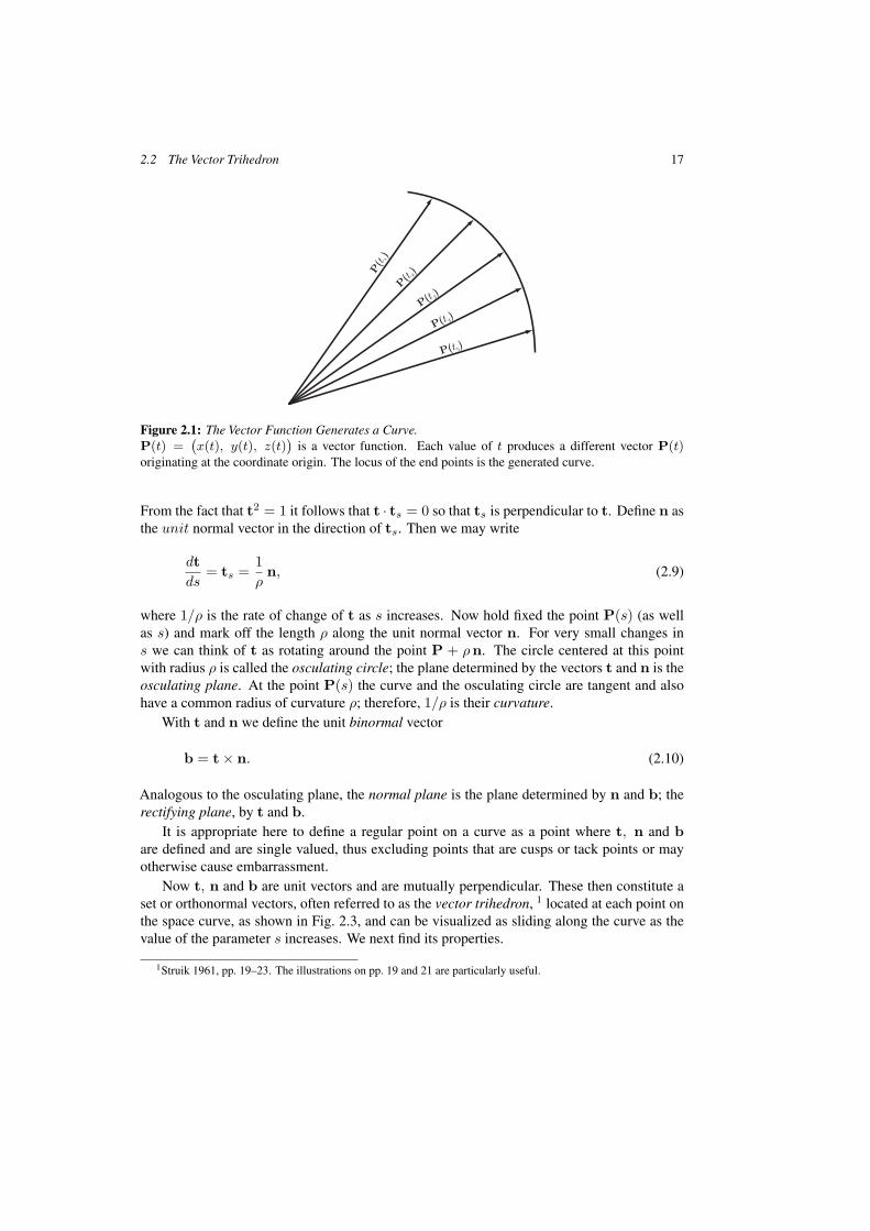
Figure 2.1: The Vector Function Generates a Curve.P(t) =
(x(t), y(t), z(t)
)is a vector function. Each value of t produces a different vector P(t)
originating at the coordinate origin. The locus of the end points is the generated curve.
From the fact that t2 = 1 it follows that t · ts = 0 so that ts is perpendicular to t. Define n asthe unit normal vector in the direction of ts. Then we may write
dtds
= ts =1ρ
n, (2.9)
where 1/ρ is the rate of change of t as s increases. Now hold fixed the point P(s) (as wellas s) and mark off the length ρ along the unit normal vector n. For very small changes ins we can think of t as rotating around the point P + ρn. The circle centered at this pointwith radius ρ is called the osculating circle; the plane determined by the vectors t and n is theosculating plane. At the point P(s) the curve and the osculating circle are tangent and alsohave a common radius of curvature ρ; therefore, 1/ρ is their curvature.
With t and n we define the unit binormal vector
b = t × n. (2.10)
Analogous to the osculating plane, the normal plane is the plane determined by n and b; therectifying plane, by t and b.
It is appropriate here to define a regular point on a curve as a point where t, n and bare defined and are single valued, thus excluding points that are cusps or tack points or mayotherwise cause embarrassment.
Now t, n and b are unit vectors and are mutually perpendicular. These then constitute aset or orthonormal vectors, often referred to as the vector trihedron, 1 located at each point onthe space curve, as shown in Fig. 2.3, and can be visualized as sliding along the curve as thevalue of the parameter s increases. We next find its properties.
1Struik 1961, pp. 19–23. The illustrations on pp. 19 and 21 are particularly useful.

18 2 Space Curves and Ray Paths
Figure 2.2: The Derivative of a Vector Function is a Tangent.Let the endpoint of P(t) be point a; that of P(t+∆t) be point b. The difference between the two vectorsis the chord α − b. As ∆t → 0 point b approaches point a. The limiting position of the chord a − b isthe tangent at point a. The limit of the quotient formed by the vector difference and the arc length of theunit tangent vector to the curve at point a; this limit is also the derivative of the vector function P withrespect to s.
2.3 The Frenet-Serret Equations
At every regular point on the curve the vector trihedron can serve as a local coordinate system;any vector through that point can be represented as a linear combination of t, n and b. We dothis with the derivative of n so that
ns = αt + βn + γb, (2.11)
where the coefficients are to be determined. Since n2 = 1, it follows that n ·ns = 0; when wemultiply Eq. 2.11 by n we see that β = 0. Since t · n = 0, its derivative must also equal zero;t ·ns + ts ·n = 0. By multiplying Eq. 2.11 by t we get t ·ns = α = −ts ·n = −1/ρ. Sincen · b = 0 its derivative gives us ns · b + n · bs = 0 which results in ns · b = γ = −n · bs.With a similar calculation with b · t we get that bs · t = −ts · b = 1/ρ. From this and thenonvanishing of n · bs we see that the change in b is also in the direction of n; b thereforefollows a twisting motion around the unit tangent vector t as it slides along the curve. We callthis rate of twist the curve’s torsion which we denote by 1/τ . Then, in Eq. 2.11, γ = −1/τ .These results constitute the Frenet-Serret equations.2 In matrix form they are
ts
ns
bs
=
0 1/ρ 0
−1/ρ 0 1/τ
0 −1/τ 0
t
n
b
(2.12)
The vector trihedron slides along the space curve, much as an airplane glides along itsflight path, moving in the direction of t, a wing as its normal vector n and with b as its verticalstabilizer (or is it the other way around?), pitching and rolling as it moves along. The rate ofroll is the torsion 1/τ ; its pitch is the curvature 1/ρ.
2Struik 1961. Chapter 1. Struik uses a different notation. κ is 1/ρ in our notation and τ is torsion rather than 1/τ .
2.4 When the Parameter is Arbitrary 19
2.4 When the Parameter is Arbitrary
Later on we will need to consider the case when the arbitrary parameter, which we will call t,cannot be transformed easily into the arc length parameter s. The relationship between thesetwo parameters is determined by a total differential equation. If its solution is not obtainableor it is extremely complicated then it is necessary to refer t, n and b back to the originalparameter t.
Refer to Eqs. 2.6, 2.8 and 2.9 and get
t = Ps = Pt
/√P2
t , (2.13)
from which comes
ts =1ρn =
1√P2
t
tt =1
(P2t )3/2
[(P2
tPtt − (Pt · Ptt)Pt
]
=Pt × (Ptt × Pt)
(P2t )3/2 ,
which reduces further to the curvature
1ρ
=1P2
t
√(Ptt × Pt)2, (2.14)
and to the unit normal vector
n =Pt × (Ptt × Pt)√P2
t
√(Ptt × Pt)2
. (2.15)
We use Eqs. 2.17 and 2.19 to get the binormal vector
b = t × n =Pt√P2
t
× Pt × (Ptt × Pt)√P2
t
√(Ptt × Pt)2
= − Ptt × Pt√(Ptt × Pt)2
. (2.16)
Finally we come to the calculation of the torsion. For this we use the third equation of Eq. 2.12for the derivative of b and take the derivative of Eq. 2.16 to get
bs =1τn =
bt√P2
t
= − (Pttt × Pt) · Ptt√P2
t
[(Ptt × Pt)2
]3/2Pt × (Ptt × Pt),
which, when compared with Eq. 2.15 yields
1τ
=(Pttt × Pt) · Ptt
(Ptt × Pt)2. (2.17)
These calculations give us curvature, torsion and the three orthogonal vectors of the trihe-dron in terms of the parameter t.
20 2 Space Curves and Ray Paths
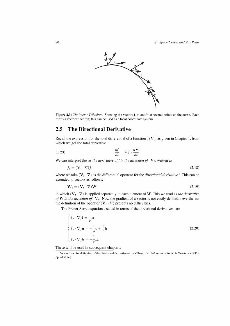
Figure 2.3: The Vector Trihedron. Showing the vectors t, n and b at several points on the curve. Eachforms a vector trihedron; this can be used as a local coordinate system.
2.5 The Directional Derivative
Recall the expression for the total differential of a function f(V), as given in Chapter 1, fromwhich we got the total derivative
(1.23)df
dt= ∇f · dV
dt.
We can interpret this as the derivative of f in the direction of Vt, written as
ft = (Vt · ∇)f, (2.18)
where we take (Vt · ∇) as the differential operator for the directional derivative.3 This can beextended to vectors as follows:
Wt = (Vt · ∇)W, (2.19)
in which (Vt · ∇) is applied separately to each element of W. This we read as the derivativeof W in the direction of Vt. Now the gradient of a vector is not easily defined; neverthelessthe definition of the operator (Vt · ∇) presents no difficulties.
The Frenet-Serret equations, stated in terms of the directional derivatives, are
(t · ∇)t =1ρn
(t · ∇)n = −1ρt +
1τb
(t · ∇)b = −1τn.
(2.20)
These will be used in subsequent chapters.3A more careful definition of the directional derivative or the Gateaux Variation can be found in Troutman(1983),
pp. 44 et seq.
2.6 The Cylindrical Helix 21
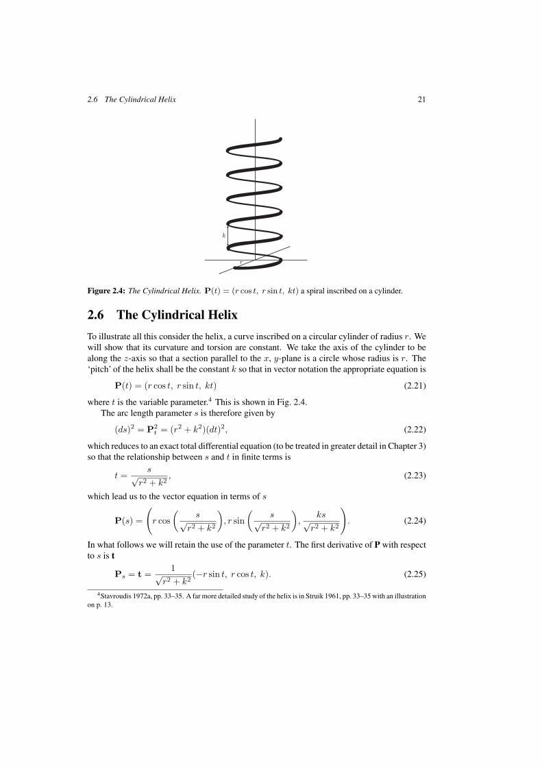
Figure 2.4: The Cylindrical Helix. P(t) = (r cos t, r sin t, kt) a spiral inscribed on a cylinder.
2.6 The Cylindrical Helix
To illustrate all this consider the helix, a curve inscribed on a circular cylinder of radius r. Wewill show that its curvature and torsion are constant. We take the axis of the cylinder to bealong the z-axis so that a section parallel to the x, y-plane is a circle whose radius is r. The‘pitch’ of the helix shall be the constant k so that in vector notation the appropriate equation is
P(t) = (r cos t, r sin t, kt) (2.21)
where t is the variable parameter.4 This is shown in Fig. 2.4.The arc length parameter s is therefore given by
(ds)2 = P2t = (r2 + k2)(dt)2, (2.22)
which reduces to an exact total differential equation (to be treated in greater detail in Chapter 3)so that the relationship between s and t in finite terms is
t =s√
r2 + k2, (2.23)
which lead us to the vector equation in terms of s
P(s) =
(r cos
(s√
r2 + k2
), r sin
(s√
r2 + k2
),
ks√r2 + k2
). (2.24)
In what follows we will retain the use of the parameter t. The first derivative of P with respectto s is t
Ps = t =1√
r2 + k2(−r sin t, r cos t, k). (2.25)
4Stavroudis 1972a, pp. 33–35. A far more detailed study of the helix is in Struik 1961, pp. 33–35 with an illustrationon p. 13.

22 2 Space Curves and Ray Paths
Its derivative is
ts =1ρn =
−r√r2 + k2
(cos t, sin t, 0), (2.26)
so that the curvature must be
1ρ
=−r√
r2 + k2, (2.27)
and the unit normal vector
n = (cos t, sin t, 0). (2.28)
From Eqs. 2.25 and 2.28 we calculate the unit binormal vector
b = t × n =1√
r2 + k2(−k sin t, k cos t, r) (2.29)
the derivative of which leads to the torsion
bs = −1τn =
−k√r2 + k2
(cos t, sin t, 0), (2.30)
so that
1τ
=−k√
r2 + k2. (2.31)
Here we have used the Frenet-Serret equations, Eq. 2.17.So, from Eqs. 2.27 and 2.31 we can see the curvature and torsion are indeed constants,
exactly as advertised.
2.7 The Conic Section
We depart from the standard representation of the conic section in the following way. We writethe equation of the ellipse in polar coordinates with a focus as the pole and the major axis asthe polar axis. Then its equation will be given in parametric form by{
y = � sin φ
z = � cos φ(2.32)
where the length of the radius vector is5
� =r
1 − ε cos φ(2.33)
5Korn and Korn. pp. 41–53. Expressions for the conic section.

2.7 The Conic Section 23
Figure 2.5: The Ellipse and its Parameters.The ellipse is given in terms of polar coordinates with the pole located at a focus and with the polar axislying along the major axis. We call the focus lying at the pole the proximal focus; the other, the distalfocus. The eccentricity is ε < 1. The angle v is the parameter on which depends the radius vector,R(v) = r/(1 − ε cos v).
The eccentricity is ε ∈ (0, 1), the semi latus rectum is r. Because of the simplicity of Eq. 2.33the use of eccentricity is preferable to the conic constant, the quantity usually encountered inoptics.When v = 0, � is the distance from the coordinate origin, along the polar axis, to a
vertex of the ellipse; �0 = r/(1 − ε). When φ = π/2, then � equals the semi latus rectum;�π/2 = r. Finally if φ = π then � equals the distance along the polar axis in a negative directionto the ellipse’s opposite vertex, �π = r/(1 + ε).
We define the proximal focus of the ellipse as the first focus encountered; in this case itlies at the origin. The distal focus is defined as the second focus. These terms will be usedextensively in Chapters 4 and 13. It follows from the results of the previous paragraph that thedistance between the proximal and the distal foci is equal to the difference
df = �0 − �π =2εr
1 − ε2(2.34)
The length of the major axis is
2 a = �0 + �π =2r
1 − ε2(2.35)
From the standard form of the ellipse we can derive the length of the semi minor axis asb = r/
√1 − ε2.
In Fig. 2.5 is shown an ellipse with these various quantities indicated. It also shows theangle φ′ and the distance �′, analogues of φ and �, but associated with the distal focus. FromEq. 2.33 it follows that
�′ =r
1 − ε cos v′ (2.36)
24 2 Space Curves and Ray Paths
so that, from Eq. 2.36, we can get
y =r sin v
1 − ε cos v=
r sin v′
1 − ε cos v′
z = 2ε − (1 + ε2) cos v = df − r cos v′
1 − ε cos v′ .
(2.37)
By substituting for df from Eq. 2.34 we are able to solve for v′ to get{sin v′ = (1 − ε2) sin v/K2
cos v′ =[2ε − (1 + ε2) cos v
]/K2
(2.38)
where
K2 = (1 + ε2) − 2ε cos v. (2.39)
Note that K2 can be written as the sum of two squares, (cos v−ε)2+sin2 v, so that the quantityis never negative and K is always real.
From Eq. 2.37 we obtain easily
�′ =rK2
(1 − ε2)(1 − ε cos v). (2.40)
These same formulas, Eqs. 2.37 and 2.38, describe the circle (ε = 0), the parabola (ε = 1),and the hyperbola (ε > 1), and therefore can be used to represent any conic section.
Now cast Eq. 2.37 into vector form
P(v) = �(0, sin v, cos v), (2.41)
the derivative of which is
Pv =r
(1 − ε cos v)2(0, cos v − ε, − sin v). (2.42)
From Eq. 2.7 we can see that P2v = (ds/dv)2 = r2K2/(1 − ε cos v)4, so that
ds
dv=
√P2
v =rK
(1 − ε cos v)2. (2.43)
Considered as an ordinary differential equation its solution involves an elliptic integral ofthe second kind, a relation too far complicated for our purposes. So we must be content withthe results of the preceding section.Recall that t=dP/ds = (dP/dφ)/(ds/dφ) so that
t =1K (0, cos v − ε, − sin v). (2.44)
From t we can deduce the unit normal vector n and the curvature 1/ρ using Eqs. 2.20 and2.44. First we calculate
tv = −1 − ε cos v
K3 (0, sin v, cos v − ε). (2.45)
2.8 The Ray Equation 25
From this and Eq. 2.43 we get
ts =1ρn =
∂t/∂v
∂s/∂v= −1 − ε cos v
K3 (0, sin v, cos v − ε), (2.46)
which lead us to
1ρ
=1r
(1 − ε cos v)2
K3 (2.47)
and
n =1K (0, sin v, cos v − ε). (2.48)
From Eq. 2.10 we get
b = t × n = (1, 0, 0). (2.49)
The explanation for this is that the ellipse is a plane curve that we have located on they, z-plane. Its b vector must therefore be a unit vector in the x direction. It also follows thatthe curve’s torsion 1/τ must equal zero.
A caution; ρ and � must not be confused. The radius of curvature of the ellipse is ρ and itscurvature is 1/ρ. The distance between a point on the ellipse and the proximal focus is �; to itsdistal focus it is �′. In Chapters 4 and 6 we will see that 1/� and 1/�′ can also be interpretedas curvatures of spherical wavefronts which we will encounter in Chapter 13. These resultswill also be applied in Chapter 4, the chapter on surfaces, to get the equation for the prolatespheroid.
2.8 The Ray Equation
In the last chapter we derived the ray equation
(1.29)d
ds
(n
dPds
)= ∇n
or, expressed another way
(1.30) nPss + (∇n · Ps)Ps = ∇n.
Recall that all derivatives are with respect to the arc length parameter s. Expressing the rayequation as in Eq. 1.30, in terms of the tangent, normal and binormal vectors, we get
n
ρn + (∇n · t)t = ∇n. (2.50)
If we multiply this by b we see that
∇n · b = 0, (2.51)
26 2 Space Curves and Ray Paths
which says that the binormal vector of a ray path at any point in an inhomogeneous mediummust always be perpendicular to that medium’s gradient at that point. Another way of sayingthis is that the vectors t, n and ∇n are coplanar.
We can rewrite Eq. 2.50 in the form
1ρn =
1nt × (∇n × t) (2.52)
by using the vector identity in Eq. A.6. Squaring this leads to an expression for the curvatureof the ray at any point
1ρ
=1n
√(∇n × t)2 (2.53)
Taking the vector product of t with Eq. 2.52 we can get
n
ρb = −(∇n × t), (2.54)
which, when differentiated with respect to s, leads to
n
ρτn +
(n
ρ
)s
b = −[(∇n)s × t
] − 1ρ(∇n × b). (2.55)
The scalar product of this with n yields to the expression for torsion at any point
1τ
=1n
[ρ(∇n)s · b + (∇n · t)]. (2.56)
2.9 More on the Fish Eye
In the last chapter we applied the Euler equations to Maxwell’s fish eye and obtained thedifferential equation for rays in that medium
(1.34) (1 + P2)Pss − 2(P · Ps)Ps + 2P = 0,
which we then differentiate to get
(1.35) (1 + P2)Psss − 2(P · Pss)Ps = 0.
The scalar product of this with Pss yields Pss · Psss = 0 which is the same as dP2ss/ds = 0,
from which P2ss = constant. From Eq. 2.9 we have that Pss = ts = (1/ρ)n so that the
curvature (1/ρ) is constant along a ray
1/ρ = constant. (2.57)
Moreover, by taking the scalar product of Eq. 1.35 with Ps × Pss, we get
Psss · (Ps × Pss) = 0. (2.58)
2.9 More on the Fish Eye 27
When this is compared with Eq. 2.17 we can see that the torsion is zero. Since the torsion iszero, rays in Maxwell’s fish eye must be planar and since they have constant curvature theymust be arcs of circles.
We can go a little further. Multiply Eq. 1.34 by Pss (recall that Ps · Pss = 0) to get
2(P · Pss) = −(1 + P2)/ρ (2.59)
When this is substituted into Eq. 1.35 we get
Psss +1ρPs = 0, (2.60)
a linear, third order ordinary differential equation with constant coefficients. Its general solutionis
P(s) = ρ(A sin(s/ρ) − B cos(s/ρ) + C
), (2.61)
where A, B, and C are vector constants of integration. Its derivative is
Ps = A cos(s/ρ) + B sin(s/ρ) (2.62)
The square of this must equal unity yielding
A2 cos2(s/ρ) + B2 sin2(s/ρ) + 2(A · B) sin(s/ρ) cos(s/ρ) = 1, (2.63)
from which we must conclude that A and B are both unit vectors and that A · B = 0. Thevectors A and B determine a plane. On this plane Eq. 2.61 provides the required solution, thearc of a circle.
What we have done in this chapter is to construct an analytic system for the study of spacecurves that, as we will see in a later chapter, is preliminary to the development of the differentialgeometry of surfaces. It is certainly incomplete. But we were able to apply it to rays paths ininhomogeneous media that led to a description of these objects in most general terms withoutneeding to look at special cases or at boundary conditions for the resulting differential equation.We will return to this later when we apply this material to the pseudo Maxwell equations.
The Mathematics of Geometrical and Physical Optics: The k-function and its Ramifications. O.N. StavroudisCopyright c© 2006 WILEY-VCH Verlag GmbH & Co. KGaA, WeinheimISBN: 3-527-40448-1
3 The Hilbert Integral and the Hamilton-Jacobi Theory
A few of the elementary problems in the Calculus of Variations were treated in Chapter 1where it was assumed that the end points of the variational integrals were fixed. When theseend points are allowed to vary the problem becomes much more difficult than merely solvingthe Euler equations. There had been no general method for solving this kind of problem but inthe later years of the nineteenth century David Hilbert did find an approach that enabled us totreat this problem in a general way. This we call the Hilbert Integral.1
The Hilbert Integral has applications that transcend the variable end point problem; thesewill be our main interest in this chapter. With it we will find an alternative proof of Snell’slaw of refraction. We will find conditions for aggregates of rays to have orthogonal surfacesor wavefronts; such aggregates we will call normal congruences or orthotomic systems. TheHilbert Integral will also lead to the Hamilton-Jacobi theory that, in an optical context, is thefoundation for modern aberration theory. It will also lead to the eikonal equation which willbe of major importance in subsequent chapters.
Recall the statement of the general variational problem that had been introduced in Chapter 1
(1.6) I =
b∫a
f(x, y(x), z(x), yx(x), zx(x)
)dx,
and its solution in terms on the Euler equations
(1.15)
d
dx
∂f
∂yx=
∂f
∂y
d
dx
∂f
∂zx=
∂f
∂z.
Also recall the steps we used, from Eq. 1.15, in Chapter 1, to get
(1.17)∂f
∂x=
d
dx
[f−yx
∂f
∂yx−zx
∂f
∂zx
].
These are second order ordinary differential equations whose general solutions consist ofa two parameter family of extremal curves that we will refer to as a field of extremals. In whatfollows we will assume that we are dealing with a region of space in which these extremals aredense.
1Bliss 1946, pp. 18–28.

30 3 The Hilbert Integral and the Hamilton-Jacobi Theory
Figure 3.1: The Hilbert Integral. C1 and C2 represent two arbitrary surfaces connected by several rays.
Take two curves, not necessarily extremals, lying in such a field. These we represent bytwo sets of functions of a single parameter
C1 : x1(u), y1(u), z1(u); C2 : x2(u), y2(u), z2(u),
so each value of u determines two points, one on each curve. We can then form a variationalintegral connecting these two points, one on each curve, so that both are functions of u. SeeFig. 3.1. Then the value of the variational integral is also a function of u
I(u) =
x2(u)∫x1(u)
f(x, y(x, u), z(x, u), yx(x, u), zx(x, u))dx. (3.1)
Here the extremals, denoted by y(x, u), z(x, u), have their end points on C1 and C2 so that
y(x1(u), u
)= y1(u), z
(x1(u), u
)= z1(u),
y(x2(u), u
)= y2(u), z
(x2(u), u
)= z2(u).
(3.2)
We next calculate the derivative of I(u)
dI
du= f
(x, y(x, u), z(x, u), yx(x, u), zx(x, u)
)∣∣∣∣x=x2(u)
dx2
du
− f(x, y(x, u), z(x, u), yx(x, u), zx(x, u)
)∣∣∣∣x=x1(u)
dx1
du(3.3)
+
x2(u)∫x1(u)
[∂f
∂yyu +
∂f
∂zzu +
∂f
∂yxyxu +
∂f
∂zxzxu
]dx.
31
The first two of these terms are written as one, (dx/du) f∣∣x=x2
x=x1. The integral is a bit more
difficult. Using the Euler equations, Eq. 1.15, and the steps used in obtaining Eq. 1.15, we gotx2(u)∫
x1(u)
[∂f
∂yyu +
∂f
∂zzu +
∂f
∂yxyxu +
∂f
∂zxzxu
]dx
=
x2(u)∫x1(u)
[yu
d
dx
∂f
∂yx+ zu
d
dx
∂f
∂zx+ yxu
∂f
∂yx+ zxu
∂f
∂zx
]dx (3.4)
=
x2(u)∫x1(u)
d
dx
[yu
∂f
∂yx+ zu
∂f
∂zx
]dx =
[yu
∂f
∂yx+ zu
∂f
∂zx
]x=x2(u)
x=x1(u).
Next note that the total derivatives of y and z with respect to u are
dy
du= yx
dx
du+ yu ;
dz
du= zx
∂x
∂u+ zu. (3.5)
Substituting for yu and zu in Eq. 3.4 yields an expression for dI/du,
dI
du=
[f − yx
∂f
∂yx− zx
∂f
zx
]dx
du+
[∂f
∂yx
dy
du+
∂f
∂zx
dz
du
]x=x2(u)
x=x1(u). (3.6)
Now we define the Hilbert Integral along a curve C as,
J∗(C) =∫ x2
x1
{[f − yx
∂f
∂yx− zx
∂f
zx
]dx
du+
∂f
∂yx
dy
du+
∂f
∂zx
dz
du
}du, (3.7)
where (x, y, z) lies on the path of integration. Then it follows that
dI
du=
d
duJ∗(C2) − d
duJ∗(C1), (3.8)
where x(u), y(u) and z(u) are the coordinate functions of the curve C. By integrating thisequation between the limits u1 and u2 we get
I(Eb) − I(Ea) = J∗(C2) − J∗(C1), (3.9)
where Ea and Eb are two extremals that correspond to the two values u1 and u2. This is shownin Fig. 3.2.
Another definition: If the integrand of the Hilbert Integral should vanish at a point thenthe curve C is said to be transversal to the extremal at that point; or more simply, transversalat that point. If the Hilbert integrand should vanish everywhere on C then C is said to betransversal to the field of extremals.
Note also that if the Hilbert Integral is expressed as a line integral its integrand takes theform [
f − yx∂f
∂yx− zx
∂f
∂zx
]dx +
∂f
∂yxdy +
∂f
∂zxdz, (3.10)

32 3 The Hilbert Integral and the Hamilton-Jacobi Theory
Figure 3.2: The Hilbert Integral. C1 and C2 are two surfaces connected by the pair of rays Eb and Ea.The Hilbert Integral, calculated around the closed path Eb, C2, Ea, C1, must equal zero.
a total differential. It follows that if a curve C is to be transversal to the field of extremals thena total differential equation must be satisfied. Going further, the existence of a solution to thistotal differential is a necessary and sufficient condition for the existence of a transversal.
3.1 A Digression on the Gradient
First of all a clarification. Some authors use ∇ as the differential operator whose componentsare partial derivatives with respect to a Cartesian coordinate system and use grad, curl and divto represent operators whose derivatives are with respect to different coordinate axes. Herewe do not make that distinction; ∇ will denote such an operator under any coordinate system.For example, the gradient of a function F , ∇F , will always represent a vector perpendicularto the surface F = constant.
Now consider the integral of the gradient of F , ∇F , along a curve P(t)(0 ≤ t ≤ 1) fromthe point P0 = P(0) to P1 = P(1)
∫ P1
P0
∇F · dP =∫ 1
0∇F · dP
dtdt.
This integrand can be written as a directional derivative as defined in Eq. 2.23 and the integralbecomes∫ 1
0(Pt · ∇)F dt =
∫ 1
0
dFdt
dt = F(P1) − F(P0).
Notice that the value of the integral depends only on the value of F at the two end points andnot on the path P(t) of the integral. We conclude that the integral of a gradient is independentof the path of integration. As a consequence, the integral of a gradient about a closed path mustequal zero.2∮
∇F · dP = 0. (3.11)
2Bliss 1946, Chapter III.
3.2 The Hilbert Integral. Parametric Case 33
3.2 The Hilbert Integral. Parametric Case
Here we apply the vector notation in which the variational integral takes the form
(1.24) I =∫ t2
t1
f(P, Pt)dt,
as shown in Chapter 1 so that the Euler equation becomes
(1.26)d
dt∇tf = ∇f.
As before, let the two curves be C1 : V(u) and C2 : W(u) and construct a family of extremals,P(t, u), that connect the two. Then
P(t1, u) = V(u), P(t2, u) = W(u),
Pt(t1, u) = Vt(u), Pt(t2, u) = Wt(u).(3.12)
Then the variational integral again becomes a function of u
I(u) =∫ t2
t1
f(P(t, u), Pt(t, u)
)dt, (3.13)
and its derivative is then
dI
du=
∫ t2
t1
[∇f · dP
du+ ∇tf · dPt
du
]dt
=∫ t2
t1
[(d
dt(∇tf)
)· ∂P
du+ ∇tf ·
(d
dt
∂P∂u
)](3.14)
=∫ t2
t1
d
dt
[∇tf · ∂P
∂u
]dt =
[∇tf · ∂P
∂u
]t2
t1
.
Expanding this out gives us
dI
du= ∇tf
(P(t2, u),Pt(t2, u)
) · ∂P(t2, u)∂u
− ∇tf(P(t1, u),Pt(t1, u)
) · ∂P(t1, u)∂u
(3.15)
= ∇tf(W, Wt
) · dWdu
− ∇tf(V, Vt
) · dVdu
.
Proceeding exactly as before, we integrate to get
I(u2) − I(u1) = J∗(W) − J∗(V), (3.16)
where
J∗(V) =∫ u2
u1
∇tf(V, Vt) · Vu du, (3.17)
34 3 The Hilbert Integral and the Hamilton-Jacobi Theory
is the Hilbert Integral over the curve V. This also may be expressed as a line integral
J∗(V) =∫ V2
V1
∇tf(V, Vt) · dV. (3.18)
The integrand in Eqs. 3.17 and 3.18 is then a gradient and therefore its integral around aclosed curve must be zero as indicated in Eq. 3.11.
3.3 Application to Geometrical Optics
In the optical context the variational integral, given in Eq. 1.24, becomes
I =∫
n(P)√
P2t dt, (3.19)
so that
f = n(P)√
P2t , ∇f =
√P2
t ∇n(P), ∇tf = n(P)Pt√P2
t
, (3.20)
and the Euler equation becomes the ray equation, from Chapter 1,
(1.29)d
ds
(n
dPds
)= ∇n,
which expands to
(1.30) nPss+(∇n·Ps)Ps = ∇n.
The Hilbert Integral then becomes
J∗(V) =∫
nPs · dV. (3.21)
The integrand vanishes when Ps · dV = 0. Since Ps is tangent to the ray it must be thatV is a surface perpendicular to the ray. In this case transversality becomes orthogonality.Setting the integrand equal to zero is then tantamount to forming a total differential equationfor a surface that is perpendicular to the rays. The condition for the existence of a solutionto the equation then becomes a condition on a family of rays for which such a surface exists.Such a system is called an orthotomic system or a normal congruence.
3.4 The Condition for Transversality
Let us return to the idea of transversality, the condition where the Hilbert Integral vanishesidentically. As we can see in Eq. 3.21 in geometrical optics, a transversal curve intercepts afamily of rays at right angles. In this case the Hilbert integrand becomes a total differentialequation whose solution is a surface normal to the family of rays. In the next section we
3.5 The Total Differential Equation 35
will obtain the conditions for such a differential to be exact or differentiable and how theseconditions isolate families of rays for which an orthogonal surface exists. Then we will setthese integrands equal to zero and consider the consequences.3
The three versions of the Hilbert integrand that we have seen are the most general case
(3.7)[f−yx
∂f
∂yx−zx
∂f
zx
]dx+
∂f
∂yxdy+
∂f
∂zxdz = 0,
the parametric case
(3.18) ∇tf(V, Vt)·dV = 0,
and its application to geometric optics
(3.21) n (Ps·dV) = 0.
The barred variables pertain to coordinates on the transversal surface or, in the case ofgeometrical optics, on the orthogonal surface. The other component in each of the threeequations refers to the field of extremals; the totality of solutions to the Euler equations. Inwhat follows we will seek restrictions on the field of extremals that will assure the existenceof transversals.
3.5 The Total Differential Equation
These are all a type of differential equation generally known as a total differential equation, alinear differential form or a Pfaffian and its most general form in three dimensions is4
P dx + Q dy + R dz = 0. (3.22)
Lets assume that the solution of Eq. 3.22 is given in implicit form as, sayV (x, y, z) = 0. Compare Eq. 3.22 with the total differential of V
dV =∂V
∂xdx +
∂V
∂ydy +
∂V
∂zdz = 0, (3.23)
which gives us
∂V
∂x= P,
∂V
∂y= Q,
∂V
∂z= R. (3.24)
If V is continuous then
∂2V
∂x∂y= Py = Qx,
∂2V
∂x∂z= Pz = Rx,
∂2V
∂y∂z= Qz = Ry, (3.25)
3Stavroudis 1972a, pp. 73–76.4Bliss 1946, pp. 70–72.

36 3 The Hilbert Integral and the Hamilton-Jacobi Theory
or
Ry − Qz = 0, −Rx + Pz = 0, Qx − Py = 0. (3.26)
If we write H = (P, Q, R) then it is easy to see that Eq. 3.26 is identical to
∇ × H = 0, (3.27)
which is a condition on P, Q, and R that assures that Eq. 3.22 has a solution. This we callthe condition for exactness; Eq. 3.22 is then said to be exact.
It can happen that Eq. 3.22 is not exact but that there exists an integrating factor, µ so thatµ(Pdx + Qdy + Rdz) = 0 is then exact. Then
∂2V
∂x∂y= µPy + µyP = µQx + µxQ,
∂2V
∂x∂z= µPz + µzP = µRx + µxR, (3.28)
∂2V
∂y∂z= µQz + µzQ = µRy + µyR,
which can be rearranged into
µ(Py − Qx) = Qµx − Pµy
µ(Pz − Rx) = Rµx − Pµz
µ(Qz − Ry) = Rµy − Qµz.
(3.29)
By multiplying the first of these by R; the second, by −Q; and the third by P and adding weeliminate µ and its derivatives and get
P (Ry − Qz) + Q(−Rx + Pz) + R(Qx − Py) = 0, (3.30)
which we will call the condition for integrability. In vector form it is
H · (∇ × H) = 0. (3.31)
Now we apply this to the Hilbert integrand and refer back to Eq. 3.7
H =([
f − yx∂f
∂yx− zx
∂f
zx
],
∂f
∂yx,
∂f
∂zx
), (3.32)
and to the application to geometrical optics, Eq. 3.21
H = ∇tf(V, Vt). (3.33)
Later we will use Eq. 3.33 and the condition for integrability Eq. 3.31 to get the Hamilton-Jacobi equations on which modern dynamical mechanics and geometrical optics are based.
3.6 More on the Helix 37
From the Euler equations we can show that if the equation is integrable then the index ofrefraction function, n(P) is an integrating factor for Eq. 3.22. The condition for integrabilityis of course
Ps · (∇ × Ps) = 0. (3.34)
Note first of all that
∇ × (nPs) = ∇n × Ps + n(∇ × Ps). (3.35)
By multiplying Eq. 3.34 by n we get the following:
Ps · [n(∇ × Ps)] = Ps · [∇ × (nPs) − ∇ × Ps]
= t · ∇ × (nPs) = 0.(3.36)
Take the derivative of this with respect to s to get
d
ds[t · ∇ × (nPs)] = ts · ∇ × (nPs) + t · ∇ ×
[d
ds(nPs)
]
=1ρN · ∇ × (nPs) + t · ∇ × (∇n) = 0,
(3.37)
where we have used Eq. 1.29. Since the curl of a gradient is zero this reduces to
N · ∇ × (nPs) = 0. (3.38)
Taking another derivative yields[−1
ρt +
1τb]
· [∇ × (nPs)] = 0. (3.39)
whence comes
b · ∇ × (nPs) = 0, (3.40)
which shows that all three components of ∇× (nPs) vanish so that the condition for exactnessis satisfied.
These calculations form the basis for further relations which I have called the pseudoMaxwell equations which we will see in Chapter 13.
3.6 More on the Helix
Perhaps an example will make clear the use of the Hilbert Integral. Consider again the problemthat we encountered in Chapter 2; finding the shortest distance from a fixed point to thecylindrical helix. To keep things simple we do not use the equation for the helix that involves

38 3 The Hilbert Integral and the Hamilton-Jacobi Theory
Figure 3.3: The Helix and the Hilbert Integral. Showing lines from a point A to the helix at P(t1) andP(t2). The Hilbert Integral about the closed loop A, P(t1), P(t2), A is zero.
the arc length parameter s, Eq. 2.24, but the earlier version, Eq. 2.21, that uses only the arbitraryparameter t
(2.21) P(t) = (r cos t, r sin t, kt).
Place the fixed point A on the x-axis a distance h from the origin so that A = hX, asshown in Fig. 3.3. Then the vector from this point to the helix is
Q(t) = hX − P(t), (3.41)
whose length is
l(t) =√(
hX − P(t))2
. (3.42)
The vector Q(t) is therefore a solution to the variational problem whose integral is∫
ds =∫(ds/dt)dt =
∫ √Q(t)2 dt. The Hilbert Integral that we will use will be based on this
variational integral.Now take two points on the helix corresponding to the two parameter values t1 and t2 and
form the closed loop from A to P(t1) to P(t2) then back to A. Because the loop is closedthe Hilbert Integral calculated over this loop must be zero. Moreover, the Hilbert Integralcalculated on Q(t1) and Q(t2), because they are extremals, degenerate to variational integrals,as shown in, say, Eq. 3.16. If we backtrack to Eq. 3.8, from which Eqs. 3.9 and 3.16 are derived,recalling that our loop has only three sides, we get
dI
dt=
d
dtJ∗(P(t)
). (3.43)
Now note two things. First, for the distance from A to the helix to be a minimum the derivativeof I must vanish. And second, the derivative of J∗ is simply the integrand of the Hilbert
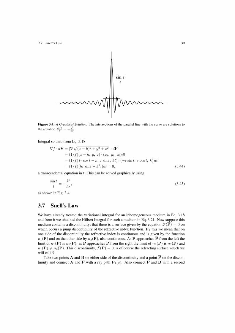
3.7 Snell’s Law 39
Figure 3.4: A Graphical Solution. The intersections of the parallel line with the curve are solutions tothe equation sin t
t= − k2
hr.
Integral so that, from Eq. 3.18
∇f · dV = [∇√
(x − h)2 + y2 + z2] · dP
= (1/f)(x − h, y, z) · (xt, yt, zt)dt
= (1/f) (r cos t − h, r sin t, kt) · (−r sin t, r cos t, k) dt
= (1/f)(hr sin t + k2t)dt = 0, (3.44)
a transcendental equation in t. This can be solved graphically using
sin t
t= −k2
hr, (3.45)
as shown in Fig. 3.4.
3.7 Snell’s Law
We have already treated the variational integral for an inhomogeneous medium in Eq. 3.18and from it we obtained the Hilbert Integral for such a medium in Eq. 3.21. Now suppose thismedium contains a discontinuity; that there is a surface given by the equation F(P) = 0 onwhich occurs a jump discontinuity of the refractive index function. By this we mean that onone side of the discontinuity the refractive index is continuous and is given by the functionn1(P) and on the other side by n2(P), also continuous. As P approaches P from the left thelimit of n1(P) is n1(P); as P approaches P from the right the limit of n2(P) is n2(P) andn1(P) �= n2(P). This discontinuity, F(P) = 0, is of course the refracting surface which wewill call S.
Take two points A and B on either side of the discontinuity and a point P on the discon-tinuity and connect A and P with a ray path P1(s). Also connect P and B with a second

40 3 The Hilbert Integral and the Hamilton-Jacobi Theory
ray path P2(s). These are, of course, extremals. Let I1 and I2 be the optical path lengths ofthe two curves determined by the appropriate variational integrals. Figure 3.5 is an attempt toshow this. Let the ‘prime’ symbol indicate derivatives with respect to s. It follows that P′
1 andP′
2 are tangent vectors to the two curves and that P′1 and P
′2 are their tangent vectors at the
point of incidence on either side of the refracting surface. Then the total optical path lengthfrom A to B is given by
I = I1 + I2. (3.46)
If A and B are not conjugates then the ray path connecting the two is unique and its opticalpath length must be an extremum relative to all other possible paths connecting the two points.Let V be any curve on S. Then the differentials of I1 and I2 along V are
dI1 = n1P′1 · dV, dI2 = −n2P
′2 · dV, (3.47)
where n1 = n1(P) and n2 = n2(P). Each of these is a Hilbert integrand representing thedifferential of optical path length. The differential of the total optical path length between Aand B, a quantity that must equal zero in order to conform to Fermat’s principle, is as follows:
dI = (n1P′1 − n2P
′2) · dV = 0.
The differential dV is tangent to the curve V. It follows that the vector n1P′1 −n2P
′2 must be
perpendicular to V. This must be true for all curves V on passing through P on S. It followsthat n1P
′1 − n2P
′2 must be parallel to the unit normal vector to S at P. Let this vector be N.
Then, for some factor k it must be that n1P1 − n2P2 = kN or
(n1P′1 − n2P
′2) × N = 0,
which becomes very quickly the vector form of Snell’s law
n1(P′1 × N) = n2(P
′2 × N). (3.48)
Recall that the absolute value of the vector product of two unit vectors is equal to the sineof the subtended angle so that |P′
1 ×N| = sin i and |P′2 ×N| = sin r, i and r being the angles
of incidence and refraction. This leads to the scalar form of Snell’s law
n1 sin i = n2 sin r, (3.49)
to which must be added the fact that P′1, P
′2 and N must be coplanar. This comes from Eq. 3.49.
This plane is called the plane of incidence.A matter of notation. In Chapter 7 in which ray tracing is studied we will use a different
notation. Equation 3.48 then becomes
n1(S1 × N) = n2(S2 × N). (3.50)
We will use these results in subsequent chapters but in a slightly different form. We willuse the reduced direction cosine vector or the reduced ray vector S = n P so that Eq. 3.48becomes
S1 × N = S2 × N. (3.51)
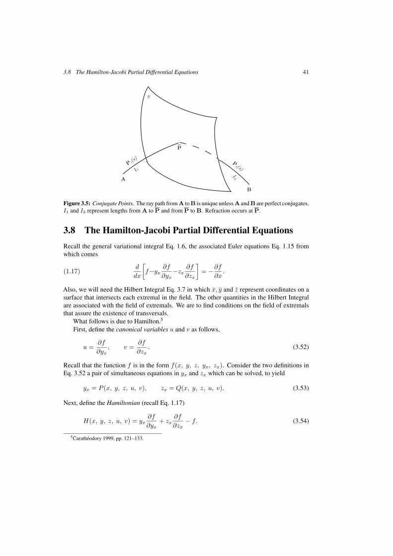
3.8 The Hamilton-Jacobi Partial Differential Equations 41
Figure 3.5: Conjugate Points. The ray path from A to B is unique unless A and B are perfect conjugates.I1 and I2 represent lengths from A to P and from P to B. Refraction occurs at P.
3.8 The Hamilton-Jacobi Partial Differential Equations
Recall the general variational integral Eq. 1.6, the associated Euler equations Eq. 1.15 fromwhich comes
(1.17)d
dx
[f−yx
∂f
∂yx−zx
∂f
∂zx
]= −∂f
∂x.
Also, we will need the Hilbert Integral Eq. 3.7 in which x, y and z represent coordinates on asurface that intersects each extremal in the field. The other quantities in the Hilbert Integralare associated with the field of extremals. We are to find conditions on the field of extremalsthat assure the existence of transversals.
What follows is due to Hamilton.5
First, define the canonical variables u and v as follows,
u =∂f
∂yx, v =
∂f
∂zx. (3.52)
Recall that the function f is in the form f(x, y, z, yx, zx). Consider the two definitions inEq. 3.52 a pair of simultaneous equations in yx and zx which can be solved, to yield
yx = P (x, y, z, u, v), zx = Q(x, y, z, u, v). (3.53)
Next, define the Hamiltonian (recall Eq. 1.17)
H(x, y, z, u, v) = yx∂f
∂yx+ zx
∂f
∂zx− f. (3.54)
5Caratheodory 1999, pp. 121–133.
42 3 The Hilbert Integral and the Hamilton-Jacobi Theory
Using Eqs. 3.52 and 3.53 it is clear that this can also be written as
H(x, y, z, u, v) = Pu + Qv − f. (3.55)
The total differential of the Hamiltonian is
dH =∂H
∂xdx +
∂H
∂ydy +
∂H
∂zdz +
∂H
∂udu +
∂H
∂vdv, (3.56)
but by using Eq. 3.55 we get
dH = P du + u dP + Q dv + v dQ
−[∂f
∂xdx +
∂f
∂ydy +
∂f
∂zdz +
∂f
∂yxdyx +
∂f
∂zxdzx
]= P du + u dP + Q dv + v dQ (3.57)
−[∂f
∂xdx +
∂f
∂ydy +
∂f
∂zdz + u dP + v dQ
]
= Pdu + Qdv −[∂f
∂xdx +
∂f
∂ydy +
∂f
∂zdz
],
where we have used Eq. 3.53. By equating coefficients of corresponding differentials we get
∂H
∂x= −∂f
∂x, (3.58)
which we already have from Eq. 1.17, and
∂H
∂y= −∂f
∂y= − d
dx
∂f
∂yx=
du
dx,
∂H
∂u= P = yx =
dy
dx,
∂H
∂z= −∂f
∂z= − d
dx
∂f
∂zx=
dv
dx,
∂H
∂v= Q = zx =
dz
dx,
(3.59)
where we have used Eqs. 3.52 and 3.53. These are called the canonical equations.Now return to the Hilbert integrand from Eq. 3.7. When this is set equal to zero we have
the total differential equation for the transversal surface
−Hdx + udy + vdz = 0. (3.60)
The first two of the canonical equations, Eq. 3.59, satisfy the condition that Eq. 3.60 be exact.Then there must exist a solution to Eq. 3.60, a function φ such that
∂φ
∂x= −H(x, y, z, u, v),
∂φ
∂y= u,
∂φ
∂z= v. (3.61)
By elimination u and v from the first equation in Eq. 3.61 yields the Hamilton-Jacobi partialdifferential equation for the transversal surface
∂φ
∂x+ H
(x, y, z,
∂φ
∂y,
∂φ
∂z
)= 0. (3.62)
3.9 The Eikonal Equation 43
3.9 The Eikonal Equation
This is much simpler. Recall the Hilbert integrand expressed in the context of geometricaloptics, Eq. 3.21
nPs · dV = 0,
and its condition for exactness from Eq. 3.27
∇ × (nPs) = 0. (3.63)
Since the curl of a gradient always equals zero there must exist a function φ such that
nPs = ∇φ, (3.64)
where φ(P) = constant is the equation of the transversal surface or, in this case, the orthogonalsurface, the plane of constant phase or wavefront. The function φ is referred to as Hamilton’scharacteristic function or, as I prefer, the eikonal. Recall that Ps is a unit vector in the directionof a ray; it is also the normal to the wavefront.
Now square both sides of Eq. 3.64 to get the eikonal equation, the analog to the Hamilton-Jacobi equation
(∇φ)2 = n2. (3.65)
Note that it is a non-linear partial differential equation of the first order and that it is independentof any reference to rays.
A solution to this equation, of course, would be very useful in optical design. Such asolution in the form of a power series expansion has been used in lens design for the better partof a century. Moreover it has the property that the zero order terms are exactly equivalent to theGauss-Maxwell model for a perfect lens that we will encounter in Chapter 14. The coefficientsof the terms of the power series therefore represent departures from the ideal and are termedaberrations. These terms are calculated and are shown to depend on the various parameters ofthe optical system being designed; curvatures of the refracting surfaces, separations betweenthese surfaces and the refractive indices of the constituent media.
We will depart from the power series approach and find a general solution to Eq. 3.65 infinite terms in Chapter 5.
The Mathematics of Geometrical and Physical Optics: The k-function and its Ramifications. O.N. StavroudisCopyright c© 2006 WILEY-VCH Verlag GmbH & Co. KGaA, WeinheimISBN: 3-527-40448-1
4 The Differential Geometry of Surfaces.
Any smooth surface (Smooth will be defined shortly) can be represented by a vector function intwo parameters just as a space curve can be defined by a vector function of one. Indeed we willuse space curves embedded on such a surface to reveal its properties. The ultimate objective isto apply these results to wavefront trains in homogeneous, isotropic media, whose equationswill be found in Chapter 5 as a general solution of the eikonal equation derived in Chapter 3.
In Chapter 6 the results obtained in this chapter will be used to determine the geometricproperties of these wavefronts as well as expressions for the associated caustic surfaces.
4.1 Parametric Curves1
A surface is determined completely by a vector function of two parameters, P(v, w). If wehold v fixed and allow w to vary the result is a space curve embedded on the surface. Moreaccurately, P(v0, w) is a one-parameter family of curves, with v0 as the parameter, etched onthis surface, just as P(v, w0) is a second one-parameter family of curves lying on the surface.Together, these two families of curves are referred to as the parametric curves of the surfacesuch as is shown in Fig. 4.1. Through every regular point (Again, we postpone the definitionof a term.) passes exactly two parametric curves, one from each of these two families.
These parameters are not unique. While a nonsingular transformation of the parametersresults in a different set of parametric curves on the surface the surface itself remains unchanged.We have already seen this in space curves; a change of parameterization does not change thegeometry of the curve in any way. In that case we settled on a standard parameter s, the arclength parameter, as natural and convenient. However, parameters in the vector representationof surface are not standardized.
4.2 Surface Normals
At every regular point on the surface two of these parametric curves will intersect. The partialderivatives of P with respect to the two parameters v and w, as we saw in Chapter 2, are twovectors tangent to the two parametric curves and therefore tangent to the surface. These wedenote by Pv and Pw, where the subscripts signal partial differentiation.
Now we can define smooth. We say that a surface is smooth at a point if its partial derivativesof its representative function exist, are continuous and are single valued. In addition, on a
1My favorite text in classical differential geometry, the kind used in this work, is Struik 1961. Others includeStoker 1969, Guggenheimer 1977 and Do Carmo 1976. And perhaps the best of all is Blaschke 1945.

46 4 The Differential Geometry of Surfaces.
Figure 4.1: Parametric Curves. Shown are P(v, w0) and P(v0, w), the two one-parameter families ofparametric curves. Pv and Pw are the tangent vector to these two systems of curves and Pv × Pw isthe surface normal, N.
smooth surface if the vector product Pv × Pw does not vanish at some point then that point isregular. If all points on a smooth surface are regular then the surface is said to be regular.
As an example, consider a sphere described by parametric curves that are lines of latitudeand longitude. The longitude curves are great circles. Through almost all points of the spherepass exactly two of the parametric curves; partial derivatives of the vector function describingthe sphere exist and are unique so that there is no problem with the surface normal. Howeverat the north and south poles all longitudinal curves intersect and the curve of latitude becomesa degenerate point circle. The two poles then can not be regular points. These two singularitiescan be removed by making a change of parameters but if lines of curvature are to be lines oflatitude and longitude then all that is accomplished is the relocation of the two singularities toa different pair of points.
Since Pv and Pw are tangents to the surface it follows that at every regular point theirvector product is a vector perpendicular to the surface. We then define the unit normal vectoras
N =Pv × Pw√(Pv × Pw)2
. (4.1)
This is shown in Fig. 4.1. Since N is a surface property it must be invariant under any parametertransformation.
Now let v and w be functions of a new parameter t; that is, let v = v(t) and w = w(t). Anew space curve results, one that is engraved on the surface and is defined by the vector functionP(t) = P
(v(t), w(t)
)and can be analyzed using methods from the differential geometry of
4.3 The Theorem of Meusnier 47
space curves that we encountered in Chapter 2. The tangent vector is
Pt = Pvvt + Pwwt, (4.2)
a linear combination of the two vectors tangent to the parametric curves.The differential of arc length is
(ds)2 = [Pv vt + Pw wt]2 (dt)2
= P2v (dv)2 + (Pv · Pw) dv dw + P2
w (dw)2.(4.3)
We define the first fundamental quantities to be
E = P2v, F = Pv · Pw, G = P2
w. (4.4)
These are independent of t and so they are properties of the surface and not of the inscribedcurve. Then the derivative of the arc length parameter s with respect to the parameter t becomes
ds
dt=
√E v2
t + 2F vt wt + Gw2t . (4.5)
The radicand E v2t + 2 F vt wt + Gw2
t is called the first fundamental form. This enables us tocalculated derivatives with respect to s, the arc length parameter. The unit tangent vector thenbecomes
t = Ps =Pv vt + Pw wt√
E v2t + 2 F vt wt + Gw2
t
= Pv vs + Pw ws. (4.6)
The surface unit normal vector can now be written as
N = (Pv × Pw)/D, (4.7)
where
D2 = (Pv × Pw)2 = P2vP
2w − (Pv · Pw)2 = EG − F 2. (4.8)
4.3 The Theorem of Meusnier2
We next take the derivative of the unit tangent vector with respect to the arc length parameterand obtain the unit normal vector and the curvature, as in the first of the three Frenet-Serretequations in Chapter 2
(2.20) ts =1ρn
from which we get
ts =1ρn = Pvvv2
s + 2Pvwvsws + Pwww2s + Pvvss + Pwwss. (4.9)
2Struik 1961, pp. 73–76, Do Carma 1976, pp. 142–144, Korn and Korn 1968, pp. 571–572.
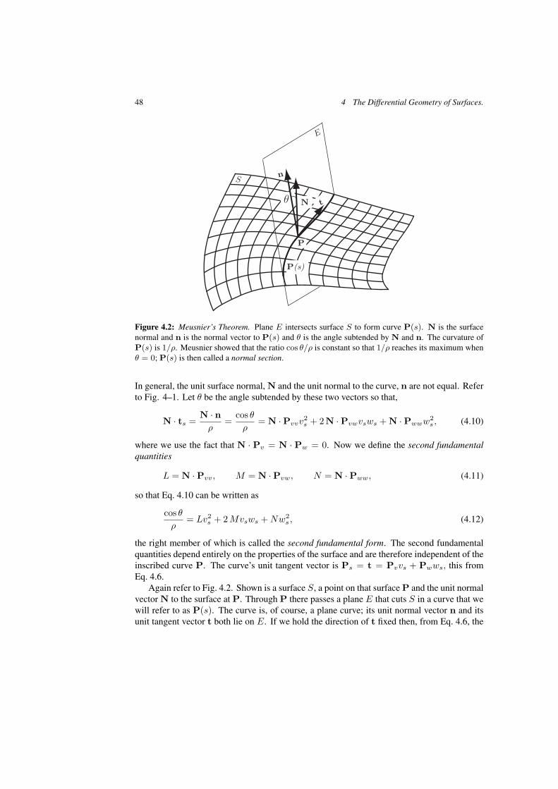
48 4 The Differential Geometry of Surfaces.
Figure 4.2: Meusnier’s Theorem. Plane E intersects surface S to form curve P(s). N is the surfacenormal and n is the normal vector to P(s) and θ is the angle subtended by N and n. The curvature ofP(s) is 1/ρ. Meusnier showed that the ratio cos θ/ρ is constant so that 1/ρ reaches its maximum whenθ = 0; P(s) is then called a normal section.
In general, the unit surface normal, N and the unit normal to the curve, n are not equal. Referto Fig. 4–1. Let θ be the angle subtended by these two vectors so that,
N · ts =N · n
ρ=
cos θ
ρ= N · Pvvv2
s + 2N · Pvwvsws + N · Pwww2s , (4.10)
where we use the fact that N · Pv = N · Pw = 0. Now we define the second fundamentalquantities
L = N · Pvv, M = N · Pvw, N = N · Pww, (4.11)
so that Eq. 4.10 can be written as
cos θ
ρ= Lv2
s + 2 Mvsws + Nw2s , (4.12)
the right member of which is called the second fundamental form. The second fundamentalquantities depend entirely on the properties of the surface and are therefore independent of theinscribed curve P. The curve’s unit tangent vector is Ps = t = Pvvs + Pwws, this fromEq. 4.6.
Again refer to Fig. 4.2. Shown is a surface S, a point on that surface P and the unit normalvector N to the surface at P. Through P there passes a plane E that cuts S in a curve that wewill refer to as P(s). The curve is, of course, a plane curve; its unit normal vector n and itsunit tangent vector t both lie on E. If we hold the direction of t fixed then, from Eq. 4.6, the
4.4 The Theorem of Gauss 49
coefficients vs and ws must also be fixed. It follows then that the entire right member of Eq. 4.12is constant; this because the second fundamental quantities represent surface properties andare not related to the orientation of the vector t.
Now rock the plane E as if it were hinged on the vector t. The value of the right memberof Eq. 4.12 remains constant. It follows that its left member also must be constant so that ρmust be proportional to cos θ. Our conclusion is that ρ attains its maximum value when θ iszero.
This is Meusnier’s Theorem. When θ = 0 and the normal n to the curve is in the samedirection as the surface normal N then the radius of curvature of the arc attains its maximumvalue. The curvature of the curve 1/ρ is then at a minimum. Such a curve formed by theintersection of a surface and a plane that contains the surface normal is called a normal section.
4.4 The Theorem of Gauss
The mechanics of Gauss’ theorem is shown in Fig. 4.3. Again we see the surface S, the pointP and the unit normal vector N. The difference now is that the plane E contains N so that thecurve P(s) is now a normal section and its normal vector n coincides with N. We rotate Eabout N just as a revolving door rotates about its axis.
Now we change the parameter back to t from s so that Eq. 4.12 becomes
1ρ
=Lv2
t + 2Mvtwt + Nw2t
Ev2t + 2Fvtwt + Gw2
t
, (4.13)
and Eq. 4.6 is again
t =Pvvt + Pwwt√
Ev2t + 2Fvtwt + Gw2
t
.
Our goal here is to find the extremum values of the curvature, 1/ρ as the plane pivots about thenormal vector N. We are to find those directions of t for which the curvature is a maximumor minimum. Now the direction of t is determined completely by the ratio λ = wt/vt which,when substituted into Eqs. 4.6 and 4.13, results in
t =Pv + Pwλ√
E + 2Fλ + Gλ2, (4.14)
and
1ρ
=L + 2Mλ + Nλ2
E + 2Fλ + Gλ2 . (4.15)
Note that if λ = 0 then t is the unit vector Pv/√
E and when λ is infinite t = Pw/√
G. It isclear that as λ assumes values over the interval (−∞, ∞) the vector t ranges over all directionsperpendicular to N; all other quantities in Eqs. 4.14 and 4.15 represent surface properties andare independent of the direction of t.

50 4 The Differential Geometry of Surfaces.
Figure 4.3: The Theorem of Gauss. N is the unit normal vector to the surface S at point P. A plane Epasses through N that intersects S in curve P(s) which is then a normal section. As E is rotated, pivotingon N, a one-parameter family of normal sections is formed. Planes E1 and E2 are two positions of thatplane and P(s1) and P(s2) are two of the resulting normal sections. Gauss showed that there are exactlytwo positions of E for which the curvature of P(s) is an extremum and that these two planes must beperpendicular. The two directions are called the principal directions. The corresponding curvatures arethe principal curvatures.
At extremum values of curvature the first derivative of Eq. 4.15 must vanish so that
d
dλ
(1ρ
)=
2(E + 2Fλ + Gλ2)2
[(E + 2Fλ + Gλ2)(M + Nλ)
−(L + 2Mλ + Nλ2)(F + Gλ)]
= 0,
(4.16)
which reduces quickly to
(E + Fλ)(M + Nλ) − (L + Mλ)(F + Gλ) = 0, (4.17)
then to
1ρ
=M + Nλ
F + Gλ=
L + Mλ
E + Fλ, (4.18)
which comes from Eq. 4.15. Equation 4.16 also leads to the quadratic polynomial in λ
(EM − FL) + (EN − GL)λ + (FN − GM)λ2 = 0, (4.19)
the solution of which is
λ± =−(EN − GL) ± R
2(FN − GM), (4.20)
4.5 Geodesics on a Surface 51
where
R2 = (EN − GL)2 − 4(EM − FL)(FN − GM)
= (EN + GL − 2FM)2 − 4(EG − F 2)(LN − M2).(4.21)
By substituting the two values of λ from Eqs. 4.20 and 4.21 into Eq. 4.14 we get twodirection vectors for which the curvature attains extremum values. They are unique to thesurface, and are given by
t± =Pv + Pwλ±√
E + 2Fλ± + Gλ2±. (4.22)
These are the two principal directions; one corresponds to the maximum value of curvature,the other to its minimum.
Consider next the two roots of the quadratic in Eq. 4.19, λ+ and λ−. Then, from anothertheorem by Gauss3 that relates the roots of a polynomial to its coefficients, we get
λ+ + λ− = − EN − GL
FN − GM, λ+ λ− =
EM − FL
FN − GM. (4.23)
Now form the scalar product of the vectors in the two principal directions and get
t+ · t− =[E + (λ+ + λ−)F + Gλ+λ−
]/H+H−. (4.24)
On substituting for the sum and product of the two λ’s, given in Eq. 4.22, we can see thatt+ · t− = 0 showing that the two principal directions must be orthogonal. This result iscertainly not intuitively obvious.
The curvatures in the two principal directions are termed, naturally enough, the principalcurvatures, obtained from Eqs. 4.15 and 4.18. There are two equivalent expressions for theseprincipal curvatures. They are
1ρ±
=M + Nλ±F + Gλ±
=L + Mλ±E + Fλ±
. (4.25)
The reciprocals, ρ±, are called the principal radii of curvature and are illustrated in Fig. 4.4.
4.5 Geodesics on a Surface
Choose any pair of points on a surface and connect them with all possible curves that can beinscribed on the surface. A geodesic curve is that curve whose arc length on the surface is anextremum. Clearly, to find geodesic curves we need to invoke the Calculus of Variations andthe vector versions of the Euler equations derived in Chapter 1
(1.26)d
dt
∇tf = ∇f.
3Struik 1961, p. 80, Korn and Korn 1968, pp. 572–574.

52 4 The Differential Geometry of Surfaces.
Figure 4.4: Principal Radii of Curvature. N is the unit normal vector to the surface S at point P. Letplanes E1 and E2 pass through N in the two principal directions and let P(s1) and P(s2) be the resultingnormal sections. The two principal centers of curvature c1 and c2 lie on N and can be thought of as thecenters of circles that best fit curves P(s1) and P(s2).
As usual f designates the variational integrand that is defined by the nature of the problem tobe solved. In this case it is the length of the curves imbedded on the surface.
Let the surface be represented by a vector function of two variables, P(v, w). A curveetched on this surface will then be P(t) = P
(v(t), w(t)
). We will use the derivative of its arc
length given Eq. 4.5 in the variational integral given in Eq. 1.6
I =∫
ds =∫ √
Ev2t + 2Fvtwt + Gw2
t dt. (4.26)
The associated Euler equations are from Eq. 1.26
d
dt
∂f
∂vt=
∂f
∂v,
d
dt
∂f
∂wt=
∂f
∂w, (4.27)
f2 = Ev2t + 2Fvtwt + Gw2
t = P2t = (ds/dt)2,
4.6 The Weingarten Equations 53
the variational integrand, from Eq. 4.26. First we calculate the two partial derivatives
f∂f
∂vt= Evt + Fwt = Pv · (Pvvt + Pwwt) = Pv · Pt
f∂f
∂v= Evv2
t + 2Fvvtwt + Gvw2t
= (Pv · Pvv)v2t + [(Pvv · Pw)
+(Pv · Pvw)]vtwt + (Pw · Pvw)w2t
= (Pvvvt + Pvwwt) · (Pvvt + Pwwt)
= Pvt · Pt.
∂f
∂vt=
Pv · Pt
f= Pv · Ps and
∂f
∂v=
Pvt · Pt
f= Pvt · Ps. (4.28)
In exactly the same way we find that
∂f
∂wt= Pw · Ps and
∂f
∂w= Pwt · Ps. (4.29)
Now we come to the two Euler equations in Eq. 4.28. The first of these is
d
dt
∂f
∂vt− ∂f
∂v=
d
dt(Pv · Ps) − (Pvt · Pt) = Pv · Pss = 0,
with a similar expression for the second. Together they are
Pv · Pss = 0, Pw · Pss = 0, (4.30)
the equations for a geodesic curve on the given surface. By multiplying the second of theseby Pv; the first by Pw and subtracting we get Pss × (Pv × Pw) = D(Pss × N) = 0. SincePss = ts = (1/ρ)n it follows that n = N. Meusnier’s theorem tells us that a geodesic mustbe a normal section.
4.6 The Weingarten Equations4
The definition of the second fundamental quantities given in Eq. 4.11 and the fact that N ·Pv =N · Pw = 0 leads us to
L = N · Pvv = −Nv · Pv
M = N · Pvw = −Nv · Pw = −Nw · Pv
N = N · Pww = −Nw · Pw.
(4.31)
4Dickson 1914, pp. 55-56, Korn and Korn 1968, pp. 55–56.
54 4 The Differential Geometry of Surfaces.
Since N is a unit vector the derivatives of N2 must vanish so that N · Nv = N · Nw = 0.This means that Nv and Nw must be perpendicular to N and therefore can be written as linearcombinations of Pv and Pw, thus
{Nv = αPv + βPw
Nw = Pv + δPw,(4.32)
where α, β, γ and δ are to be determined. The scalar product of these two equations with Pv
and Pw yield
αE + βF = −L, γE + δF = −M,
αF + βG = −M, γF + δG = −N.(4.33)
By solving these for the Greek letters and substituting the result back into the original equationsin Eq. 4.32, we get
Nv =(FM − GL)Pv + (FL − EM)Pw
EG − F 2
Nw =(FN − GM)Pv + (FM − EN)Pw
EG − F 2 .
(4.34)
These are the Weingarten equations.Now consider those parametric curves that are orthogonal; those for which Pv · Pw =
F = 0. Then the Weingarten equations specialize to
Nv = − L
EPv − M
GPw
Nw = −M
EPv − N
GPw.
(4.35)
We will consider separately the two geodesic curves through a regular point on the surface;say, P(v, w0) and P(v0, w), which must be normal sections each being a member of a one-parameter family of geodesics. First look at the curve P(v, w0) and introduce the arc lengthparameter by taking v as a function of s. The other curve, represented by P(s) = P(v(s), w0)so that the unit tangent vector in the v-direction must be vt = Ps = Pvvs. But another wayof writing vt is as Pv/
√E. It follows that vs = 1/
√E where
√E is a normalizing factor for
Pv . Using the definition in Eq. 2.15 we find the binormal vector associated with the v-curveto be vb = vt × n = (Pv/
√E) × N = −Pw/
√G. To do this recall that, from Eq. 4.7,
N = (Pv/√
E) × (Pw/√
G).Now recall the second of the Frenet-Serret equations from Chapter 2
(2.20) ns = −1ρt +
1τb

4.7 Transformation of Parameters 55
and compare it with the first Weingarten equation for orthogonal parametric curves in Eq. 4.35
ns = Nvvs = −(
L√E
Pv√E
+M√G
Pw√G)
)1√E
= −(
L
Evt − M√
EGvb
).
(4.36)
From this comes
1ρv
=L
E,
1τv
=M√EG
. (4.37)
We do the same thing for the parametric curve in the w-direction, given by P(s) =P(v0, w(s)), so that Ps = Pw ws. As before it turns out that ws = 1/
√G. Now wt =
Pw/√
G so that wb = (Pw/√
G) × N. But Pw/√
G = vb. It follows than that
wb = wt × N = (Pw/√
G) × N = −vb × N = vt = Pv/√
E. (4.38)
We return to the second Weingarten equation to get
ns = Nwws = −(
M√E
Pv√E
+N√G
Pw√G
)1√G
= −N
Gwt − M√
EGwb,
(4.39)
which gives us
1ρw
=N
G,
1τw
= − M√EG
. (4.40)
An additional result, from Eqs. 4.37 and 4.40, is that 1/τv and 1/τw are equal in magnitudebut opposite in sign. This permits us to define 1/σ
1σ
=1τv
= − 1τw
=M√EG
. (4.41)
A matter of terminology: If F = 0 everywhere then the two families of parametric curvesare orthogonal; through every regular point on the surface pass two parametric curves that areperpendicular. If F = 0 and the two orthogonal families of parametric curves are in principaldirections they are called conjugate; through every regular point passes two curves, one fromeach family, that are not only orthogonal but have tangent vectors that are in the two principaldirections at that point. We will see later on that for conjugate parametric curves M = 0.
4.7 Transformation of Parameters
As had been said many times before, a transformation of the variable parameters leaves thesurface unchanged. We have already used a kind of parameter transformation in Eq. 4.2 when
56 4 The Differential Geometry of Surfaces.
we defined a curve etched onto a surface. We do the same thing here but, instead of introducinga single curve on the surface we engrave on it a two parameter family of curves. To do thiswe introduce two new parameters, p and q, and set v = v(p, q), and w = w(p, q), so that therepresentation of the surface in terms of the new parameters is related to the old by
P(p, q) = P(v(p, q), w(p, q)
). (4.42)
So what we are doing here is simply a transformation of parameters quite like switching t ands in the discussion on space curves in Chapter 2.
The partial derivatives are{Pp = Pvvp + Pwwp
Pq = Pvvq + Pwwq.(4.43)
The transformation needs to be non singular so the Jacobian must not vanish
J = vp wq − vq wp =
∣∣∣∣∣vp vq
wp wq
∣∣∣∣∣ �= 0. (4.44)
From Eq. 4.4 we calculate the first fundamental quantities for the new system
e = P2p = E v2
p + 2F vp wp + Gw2p
f = Pp · Pq = E vp vq + F (vp wq + vq wp) + Gwp wq
g = P2q = E v2
q + 2F vq wq + Gw2q .
(4.45)
We also take the transformed differential element of area d to be
d2 = eg − f2. (4.46)
Equation 4.45 can be cast in matrix form(e f
f g
)=
(vp wp
vq wq
) (E F
F G
) (vp vq
wp wq
). (4.47)
By taking the determinant of both sides of this equation we can see that the differential elementof area in the two systems are related by
d2 = J2D2, (4.48)
where D is defined in Eq. 4.8. We can go further. Since J �= 0 we may take inverses to get
J
(vp wp
vq wq
)−1
=
(wq −wp
−vq vp
)and J
(vp vq
wp wq
)−1
=
(wq −vq
−wp vp
),
so the inverse transform is
J2
(E F
F G
)=
(wq −wp
−vq vp
) (e f
f g
) (wq −vq
−wp vp
), (4.49)
4.8 When the Parametric Curves are Conjugates 57
which leads to
J2E = ew2q − 2fwpwq + gw2
p
J2F = −evqwq + f(vpwq + vqwp) − gvpwp
J2G = ev2q − 2fvpvq + gv2
p.
(4.50)
The second derivatives of P are
Pp p = Pv v v2p + 2Pv w vp wp + Pw w w2
p + Pv vp p + Pwwp p
Pp q = Pv v vp vq + Pv w (vp wq + vq wp)
+Pw w wp wq + Pv vp q + Pwwp q
Pq q = Pv v v2q + 2Pv w vq wq + Pw w w2
q + Pv vq,q + Pwwq q,
(4.51)
so that the new second fundamental quantities, calculated using Eq. 4.11, are
l = L v2p + 2M vp wp + Nw2
p
m = L vp vq + M(vp wq + vq wp) + N wp wq
n = Lv2q + 2M vq wq + N w2
q .
(4.52)
These also can be cast in matrix form as(l m
m n
)=
(vp wp
vq wq
) (L M
M N
) (vp vq
wp wq
), (4.53)
so that the inverse transform is
J2
(L M
M N
)=
(wq −wp
−vq vp
) (l m
m n
) (wq −vq
−wp vp
), (4.54)
resulting in
J2L = lw2q − 2 mwpwq + nw2
p
J2M = −lvqwq + m(vpwq + vqwp) − nvpwp
J2N = lv2q − 2 mvpvq + nv2
p.
(4.55)
4.8 When the Parametric Curves are Conjugates
Now let’s suppose that each of these two sets of parametric curves are orthogonal so thatF = Pv ·Pw and f = Pp ·Pq are both zero. Then let us assume further that the two principaldirections are the p and q directions so that the p and q parametric curves are not only orthogonalbut conjugate as well. Then we can set
wp = λ+ vp, wq = λ− vq, (4.56)

58 4 The Differential Geometry of Surfaces.
just as we had done in preparation for the calculations in Eq. 4.14. Here λ+ and λ− are thetwo roots of the quadratic equation in Eq. 4.19 that appear in Eqs. 4.20 and 4.21.
Substituting these into the expression for m, the second equation in Eq. 4.52, we get
m = vp vq[L + 2M(λ+ + λ−) + N λ+ λ−], (4.57)
which reduces to zero when the sums and products of the two λ’s from Eq. 4.24 are used.This means that m is zero whenever the parametric curves are conjugates. This results in thefollowing equations for the two sets of first fundamental quantities, from Eqs. 4.45 and 4.50
e = Ev2
p + Gw2p J2E = ew2
q + gw2p
0 = Evpvq + Gwpwq 0 = evqwq + gvpwp
g = Ev2q + Gw2
q J2G = ev2q + gv2
p,
(4.58)
Eq. 4.52 becomes when m = 0
l = L v2p + 2M vp wp + Nw2
p
0 = L vp vq + M(vp wq + vq wp) + N wp wq
n = Lv2q + 2M vq wq + N w2
q ,
(4.59)
and Eq. 4.55 is
J2L = lw2q + nw2
p
J2M = −lvqwq − nvpwp
J2N = lv2q + nv2
p.
(4.60)
Next suppose that the angle between Pp and Pv (and therefore between Pq and Pw) is theangle θ. Then, from Eq. 4.43, and recalling that F = f = 0
Pp · Pv = Evp =√
eE cos θ
Pq · Pv = Evq =√
gE cos (π/2 + θ) = −√
gE sin θ
Pp · Pw = Gwp =√
eG cos (π/2 − θ) =√
eG sin θ
Pq · Pw = Gwq =√
gG cos θ,
(4.61)
which enables us to obtain the following relations
vp =√
e/E cos θ, wp =√
e/G sin θ,
vq = −√
g/E sin θ, wq =√
g/G cos θ,(4.62)
which satisfy the equations in Eqs. 4.45 and 4.50. Here we have used the fact that eg = J2 EGfrom Eq. 4.48.
4.8 When the Parametric Curves are Conjugates 59
The next step is to substitute the expressions in Eq. 4.62 into the equations in Eq. 4.59 toget
l
e=
L
Ecos2 θ +
N
Gsin2 θ + 2
M√EG
sin θ cos θ
0 = −(
L
E− N
G
)sin 2θ + 2
M√EG
cos 2θ
n
g=
L
Esin2 θ +
N
Gcos2 θ − 2
M√EG
sin θ cos θ,
(4.63)
to which we apply Eqs. 4.37, 4.40 and 4.41 to get
1ρp
=cos2 θ
ρv+
sin2 θw
ρw+
2σ
sin θ cos θ
1ρq
=sin2 θ
ρv+
cos2 θw
ρw− 2
σsin θ cos θ
tan 2θ =2/σ
1/ρv − 1/ρw.
(4.64)
Now we apply the relations in Eq. 4.62 to Eq. 4.60, again recalling that f = F = 0 andthat eg = J2EG from Eq. 4.48 and get
L
E=
l
ecos2 θ +
n
gsin2 θ
M√EG
=(
l
e− n
g
)sin θ cos θ
N
G=
l
esin2 θ +
n
gcos2 θ,
(4.65)
which, from Eqs. 4.37, 4.40 and 4.41 become
1ρv
=cos2 θ
ρp+
sin2 θ
ρq
1ρw
=sin2 θ
ρp+
cos2 θ
ρq
1σ
=(
1ρp
− 1ρq
)sin θ cos θ.
(4.66)
The equations in Eqs. 4.64 and 4.66 are reciprocal transforms. If 1/ρp and 1/ρq are thetwo principle curvatures then Eq. 4.66 provides 1/ρv and 1/ρw, the curvatures of a geodesiccurve whose tangent makes an angle θ with one of the principal directions. The torsion of thatcurve is then 1/σ. These relations will be most important in subsequent chapters.

60 4 The Differential Geometry of Surfaces.
4.9 When F �= 0
This is the more general case when the given system of parametric curves are not orthogonal butthe transformation is to a system in which these curves are conjugate. Refer back to Eqs. 4.45and 4.52 and set m = f = 0 to get{
E vp vq + F (vp wq + vq wp) + Gwp wq = 0
L vp vq + M (vp wq + vq wp) + N wp wq = 0.(4.67)
Once again Pp/√
e and Pq/√
g are unit vectors in the two principal directions so that we mayinvoke Eq. 4.56 and Eq. 4.67 becomes{
E + F (λ+ + λ−) + Gλ+λ− = 0
L + M (λ+ + λ−) + Nλ+λ− = 0.(4.68)
When we apply Eq. 4.24 we can see that both are satisfied.The remaining equations of Eq. 4.45 become, using this notation{
e = v2p(E + 2Fλ+ + Gλ2
+)
g = v2q (E + 2Fλ− + Gλ2
−)(4.69)
and those of Eq. 4.52 are{l = v2
p(L + 2Mλ+ + Nλ2+)
n = v2q (L + 2Mλ− + Nλ2
−).(4.70)
In terms of the p, q-parameters, which correspond to a conjugate system of parametriccurves, we may write the principal directions as unit vectors
Tp = Pp/√
e, Tq = Pq/√
g. (4.71)
Also, from Eqs. 4.37, 4.40 and 4.41, we may write the principal curvatures as
1/ρp = l/e, 1/ρq = n/g. (4.72)
So now we can start with a surface described in any system of parameters, calculate thesurface normal and the first and second fundamental quantities and then transform to a newparametric system in which the lines of curvature are conjugate by using Eqs. 4.69 and 4.70.We will use these results in Chapter 9.
Now is a good time to introduce a few new concepts. First, asymptotic directions andasymptotic curves. Suppose the second fundamental form, Eq. 4.12, is zero yielding a totaldifferential equation
Lv2t + 2Mvtwt + Nw2
t = 0, (4.73)
whose solution is an expression for an arc on the surface with the property that its curvature iszero. These are the asymptotic curves or asymptotic lines. Any straight line embedded on thesurface, as it turns out, is asymptotic.
4.10 The Structure of the Prolate Spheroid 61
A second new concept is a little strange. Suppose the first fundamental form vanishes,resulting in a differential equation for another curve embedded on the surface
E v2t + 2F vt wt + Gw2
t = 0. (4.74)
Such a curve is called an isotropic curve. But from Eq. 4.5 this means that the arc length alongsuch a curve must always be zero which is impossible for any real curve; for this reason it issometimes referred to as a null curve. An isotropic curve, if it exists, must be complex whichopens the door to some amusing speculations especially in an optical context.
Our interest here is in the way these curves, asymptotic curves and isotropic curves, canbe used to understand the geometric properties of surfaces and their ultimate application to thestructure of wavefronts and the geometric aberrations associated with an optical system. Thesewill be treated further in Chapter 6 and applied in Chapter 8.
4.10 The Structure of the Prolate Spheroid5
By rotating a conic section about one of its axes we generate a conic section of revolution. Ifthe axis of revolution is the major axis of the ellipse the surface generated is called a prolatespheroid; if it is the minor axis, the surface is an oblate spheroid. Here we will deal with onlythe prolate spheroid.
As in the case of the planar conic section described in Chapter 2 we choose a focus as thepole and the polar axis as the axis of revolution and use the polar coordinates φ, θ and . If εis the eccentricity of the generating conic and if r is its semi latus rectum, then the surface isrepresented, using a vector notation, by
P = (sin φ sin θ, sin φ cos θ, cos φ), (4.75)
where is taken from Chapter 2
(2.33) =r
1 − ε cos φ.
Clearly θ is the parameter of the rotation that generates the surface.In this way we can describe four conic surfaces of revolution; the sphere ε = 0, the prolate
spheroid ε < 1, the paraboloid of revolution ε = 1 and the hyperboloid of two sheets ε > 1.In what follows we will concentrate on the prolate spheroid although the results that we willobtain may be extended easily to the other three types of conic surfaces. As before we refer tothe focus at the pole as the spheroid’s proximal focus; the other is its distal focus.
First note that the derivative of with respect to φ is
φ =−ε sin φ
1 − ε cos φ . (4.76)
Then it can be shown that
Pφ =
1 − ε cos φ
((cos φ − ε) sin θ, (cos φ − ε) cos θ, − sin φ
)Pθ = sin φ
(cos θ, − sin θ, 0
),
(4.77)
5Struik 1961, pp. 133–136. Clegg 1968, pp. 149–152, Bolza 1961, pp. 164–166.

62 4 The Differential Geometry of Surfaces.
so that the first fundamental quantities are, from Eq. 4.4
E = P2φ =
2
(1 − ε cos φ)2 K2
F = Pφ · Pθ = 0
G = P2θ = 2 sin2 φ,
(4.78)
where from Chapter 2
(2.39) K2 = 1+ε2−2ε cos φ.
Since F = 0 the parametric curves must be orthogonal. From Eq. 4.8
D2 = EG − F 2 = 4 sin2 φ
(1 − ε cos φ)2 K2. (4.79)
From Eq. 4.1 the surface normal is the vector product of these two vectors
Pφ × Pθ =− 2 sin φ
1 − ε cos φ
(sin φ sin θ, sin φ cos θ, cos φ − ε
). (4.80)
Division by D results in the unit normal vector to the surface
N = − 1K
(sin φ sin θ, sin φ cos θ, cos φ − ε
). (4.81)
To calculate the second fundamental quantities we need the derivatives of N . These are
Nφ = − 1K
(cos φ sin θ, cos φ cos θ, − sin φ
)+
Kφ
K2 N
Nθ = − sin φ
K(cos θ, − sin θ, 0
),
(4.82)
and the second fundamental quantities are, since Pφ · N = Pθ · N = 0
L = −Nφ · Pφ =
KM = −Nφ · Pθ = −Nθ · Pφ = 0
N = −Nθ · Pθ = sin2 φ
K .
(4.83)
Here we have used Eqs. 4.11 and 4.32. We know from this that the parametric curves areconjugates since M = 0.
The first task is to substitute for the first and second fundamental quantities in the quadraticequation from Eq. 4.19 whose solutions are found in Eqs. 4.20 and 4.21. Since both F = 0
4.10 The Structure of the Prolate Spheroid 63
and M = 0, Eq. 4.19 is ephemeral and we may take as its roots λ+ = 0 and λ− = ∞. Theprincipal directions given as unit vectors, from Eq. 4.22, are then
T+ =
Pφ√E
=1K
((cos φ − ε) sin θ, (cos φ − ε) cos θ, − sin φ
)T− =
Pθ√G
= (cos θ, − sin θ, 0).(4.84)
Now we come to the calculation of the principal curvatures for which we use Eq. 4.25
1ρ+
=L
E=
(1 − ε cos φ)2
K3
1ρ−
=N
G=
1 K ,
(4.85)
from which comes, using Eq. 2.43
ρ+ =rK3
(1 − ε cos φ)3
ρ− =rK
1 − ε cos φ.
(4.86)
Next we find the principal centers of curvature. We start at P and move a distance ρ±along the unit normal vector N to get D± using the equation
D± = P + ρ±N. (4.87)
We calculate first D− using Eqs. 4.71, 4.76 and 2.42 as well as the expression for ρ fromEq. 2.27 and get
D− =rε
1 − ε cos φZ = ε Z, (4.88)
where Z is the unit vector along the positive polar axis.The other principal center of curvature D+ is more complicated. To make life easier first
note that N = (−1/K)[(1/ )P − εZ
]this from Eq. 4.81. Then from Eq. 4.87 we can get
D+ = P −(
K2
(1 − cos φ)2
) (1 P − εZ
)
=1
(1 − ε cos φ)2
{[(1 − ε cos φ)2 − K2]P + ε K2Z
}=
1(1 − ε cos φ)2
[K2 D− − ε2 sin2 φP],
(4.89)
where K is given in Eq. 2.39 and P, in Eq. 4.75. These results will be used in Chapters 7and 13.
Notice that one of these points D− lies on the z-axis, the axis of rotational symmetry, justas one would expect for a rotationally symmetric surface. The surface D is, of course, thetwo-surfaced evolute of the prolate spheroid.

64 4 The Differential Geometry of Surfaces.
4.11 Other Ways of Representing Surfaces
In this chapter we have concentrated on surfaces that are represented by functions of twoparameters. Now is the time to consider alternatives. We can represent surfaces explicitly,where one of the coordinates is given as a function of the other two, or implicitly, where thesurface is given as a function of all three coordinates that is set equal to a constant.
In the first instance suppose that z is given as a function of x and y, z = z(x, y). We canuse the parametric representation of the surface where the parameters are now x and y so thatso that we can use Eq. 4.1 to calculate the surface normal. If we revert to the vector notationwe have
P(x, y) =(x, y, z(x, y)
)(4.90)
so that the two partial derivatives are then{Px =
(1, 0, zx
)Py =
(0, 1, zy
),
(4.91)
and their vector product is
Px × Py = −(zx, zy, −1
)(4.92)
which must be a surface normal. The unit normal vector must then be
N = − 1√1 + z2
x + z2y
(zx, zy, −1
). (4.93)
The other possibility is that the surface is defined by a function of three coordinates
f(x, y, z
)= constant. (4.94)
We can interpret this equation as defining implicitly the function z = z(x, y) so that the totalderivatives are
df
dx≡ ∂f
∂x+
∂f
∂z
∂z
∂x= 0
df
dy≡ ∂f
∂y+
∂f
∂z
∂z
∂y= 0.
(4.95)
Reverting to the subscript notation for derivatives we can see that this is equivalent to{zx = −fx/fz
zy = −fy/fz.(4.96)
When these are substituted back into Eq. 4.93 we get
N =1√
f2x + f2
y + f2z
(fx, fy, fz
)(4.97)

4.11 Other Ways of Representing Surfaces 65
which is exactly the normalized gradient of f
N =∇f√(∇f)2
, (4.98)
just as it should be.
This concludes the chapter on the Differential Geometry of Surfaces in which we derivedsome of the general characteristics of surfaces represented by a vector function of two param-eters. These include principal curvatures and principal directions, the properties of embeddedgeodesic curves, the Weingarten equations and the transformation of parameters. As an exam-ple, we looked at the conic section of revolution to which we will refer later. The treatment iscertainly not complete but sufficient for out needs in subsequent chapters.

The Mathematics of Geometrical and Physical Optics: The k-function and its Ramifications. O.N. StavroudisCopyright c© 2006 WILEY-VCH Verlag GmbH & Co. KGaA, WeinheimISBN: 3-527-40448-1
5 Partial Differential Equations of the First Order
In Chapter 3 we derived the eikonal equation (Eq. 3.65) from Fermat’s principle of least time.The Hilbert Integral from the Calculus of Variations was introduced which led to the Hamilton-Jacobi theory of image formation. We also derived the eikonal equation for homogeneous,isotropic media and obtained its general solution which will be the subject of this chapter.
The vector form of the eikonal equation as derived previously is
(3.65) (∇φ)2 = n2,
which can be expressed in scalar form as
(∂φ
∂x
)2
+(
∂φ
∂y
)2
+(
∂φ
∂z
)2
= n2, (5.1)
clearly a non linear first order partial differential equation.As always we will begin with simpler problems, then generalize to the more difficult. Here
we will begin with linear first order partial differential equations, with as much generality as isappropriate, using the method of Lagrange, 1 then proceed to specialize our results to non linearequations by applying the method of Lagrange and Charpit as extended by Jacobi. 2 We willdevelop general solutions for both linear and non linear equations. Using these methods wewill then find solutions to Eq. 5.1 and apply them to geometrical optics. We will not considermethods other than these nor will we look at boundary value problems.
Just as general solutions of first order ordinary differential equations involve no more thanone constant of integration, solutions of first order partial differential equations contain nomore than one arbitrary function, the number of parameters of which is one less than thenumber of independent variables in the differential equation. We will use this fact later whenwe derive a general solution from a complete integral.
Recall that the eikonal is the optical path length from some arbitrary, fixed object point,through the optical system, to some point in image space. The coordinates of that point inimage space are the arguments of the eikonal function. The coordinates of the point in objectspace do not enter these calculations and shall be ignored.
Setting the general solution of the eikonal equation equal to a constant yields an expressionfor the locus of points that have equal optical path lengths to the object point; in other words,a surface of constant phase or a wavefront.
1Forsyth 1959, Vol. V Chapter I. Garabedian 1998, pp. 6–16.2Forsyth 1959, Vol. V, pp. 55–89 Chapters VI and VIII. Forsyth 1996, pp. 392–407. Garabedian 1998, pp. 18–24.
Cohen 1933, pp. 250–253.
68 5 Partial Differential Equations of the First Order
To get this general solution we need to go through a number of steps, each of which willbe examined and explained as we proceed. Many of these steps will prove to be useful insubsequent chapters.
We have already encountered the total differential equation in Chapter 3. Here we will firstlook at the linear first order partial differential equation, then for the non linear case we willlook at the bilinear concomitant which will lead us to the method of Lagrange and Charpit asmodified by Jacobi. This leads to a solution called the complete integral which we then convertto the general solution.
This we will apply to the eikonal equation. If we set the general solution equal to an opticalpath length we introduce yet another parameter s representing the geometric distance betweensuccessive wavefronts and with this additional parameter we get an expression for a wavefronttrain.
5.1 The Linear Equation. The Method of Characteristics
This is also known as the method of Lagrange; 3 it has to do with equations in the form
P∂φ
∂x+ Q
∂φ
∂y+ R
∂φ
∂z= S, (5.2)
linear, first order partial differential equations. (Of course such an equation can contain anynumber of independent variables but for the sake of convenience here we use only three.)
If S = 0 the equation is called homogeneous; otherwise, it is inhomogeneous. Considerthe homogeneous case first
P∂φ
∂x+ Q
∂φ
∂y+ R
∂φ
∂z= 0, (5.3)
and assume that φ(x, y, z) = 0 is a solution. By comparing Eq. 5.3 with the total differentialof φ
dφ =∂φ
∂xdx +
∂φ
∂ydy +
∂φ
∂zdz = 0. (5.4)
we can see that they are proportional; that there exists a function µ such that
dx = Pdµ dy = Qdµ dz = Rdµ. (5.5)
By eliminating µ we get the characteristic equations
dx
P=
dy
Q=
dz
R. (5.6)
Equation 5.6 can be generalized to equations involving any number of independent variables.Equation 5.6 consists of no more than two total differential equations. Generally, the
number of total differential equations is one less that the number of independent variables.3Cohen 1933, pp. 15, 34–36. Korn and Korn 1968, pp. 101–102.

5.1 The Linear Equation. The Method of Characteristics 69
Each has solutions; these must be functionally independent; between them there can be nofunctional relationship. (In the more general case no characteristic can be a function of any ofthe others.) These solutions are called characteristic functions or, more simply, characteristics.The general solution of Eq. 5.2 is an arbitrary function of these two characteristics.
A very useful trick for finding characteristics comes from Eq. 5.5. If there exists functionsα, β, and γ such that
αP + βQ + γR = 0 (5.7)
then
αdx + βdy + γdz = 0. (5.8)
These two relationships lead to a method for forming linear combinations of the characteristicequations in order to simplify the process of integration.
Consider the following trivial example
x∂φ
∂x+ y
∂φ
∂y+ z
∂φ
∂z= 0.
The characteristic equations are
dx
x=
dy
y=
dz
z,
which yields the two independent total differential equations
ydx − xdy = 0, zdy − ydz = 0,
the solutions of which are the two characteristics
α = y/x, β = z/y,
so that the general solution is
φ = φ(α, β) = φ(y/x, z/y).
Calculating the partial derivatives of φ and plugging them into the original differential equationshows that it is indeed a solution.
Now for the inhomogeneous case
P∂φ
∂x+ Q
∂φ
∂y+ R
∂φ
∂z= S.
Suppose the solution is an implicit function, ψ(φ, x, y, z) = constant. Then its partialderivatives are
∂ψ
∂x+
∂ψ
∂φ
∂φ
∂x= 0,
∂ψ
∂y+
∂ψ
∂φ
∂φ
∂y= 0,
∂ψ
∂z+
∂ψ
∂φ
∂φ
∂z= 0, (5.9)
70 5 Partial Differential Equations of the First Order
which gives us
∂φ
∂x= −∂ψ
∂x
/∂ψ
∂φ,
∂φ
∂y= −∂ψ
∂y
/∂ψ
∂φ,
∂φ
∂z= −∂ψ
∂z
/∂ψ
∂φ, (5.10)
which, when inserted into the original equation yields
P∂ψ
∂x+ Q
∂ψ
∂y+ R
∂ψ
∂z+ S
∂ψ
∂φ= 0, (5.11)
a homogeneous equation in four independent variables. Thus the problem is reduced to onealready solved.
5.2 The Homogeneous Function
The word homogeneous crops up, confusingly, in a number of distinctly different contexts; as alinear homogeneous partial differential equation, as a homogeneous optical medium and alsoas the homogeneous function that we encountered in Chapter 1.
From Eq. 1.19 recall that a function f(x, y, z) is said to be homogeneous if, for everyconstant λ, f(λx, λy, λz) = λ f(x, y, z). The derivative of this with respect to λ is
x∂f
∂x+ y
∂f
∂y+ z
∂f
∂z= f, (5.12)
an inhomogeneous partial differential equation to which we may apply the results of the previoussection, in particular Eq. 5.11, which we use to get the characteristic equations
dx
x=
dy
y=
dz
z=
df
f(5.13)
which leads us to the three total differential equations
z dx − x dz = 0, z dy − y dz = 0, z df − f dz = 0, (5.14)
that lead to the three characteristics
α = x/z, β = y/z, γ = f/z, (5.15)
so that the general solution must be
F(α, β, γ) = F(x/z, y/z, f/z) = constant, (5.16)
in which f is defined implicitly. In principle we can solve this for f and get
f = z G(x/z, y/z), (5.17)
where G is another arbitrary function. This indeed does satisfy Eq. 5.12 and it also satisfiesthe definition of the homogeneous function.

5.3 The Bilinear Concomitant 71
5.3 The Bilinear Concomitant
For the moment, only as a matter of convenience, let us restrict ourselves to partial differentialequations with only two independent variables. Let z be the dependent variable and let p =∂z/∂x and q = ∂z/∂y be its partial derivatives. What follows can easily be generalized toany countable number of independent variables.4
Suppose we have a non linear, first order partial differential equation in the form
F(x, y, z, p, q) = 0, (5.18)
for which we seek a solution. Its helpful to think of F as a function of the five independentvariables x, y, z, p and q, forgetting for the moment that p and q are themselves partialderivatives of z.
Suppose further that there is a second differential equation
G(x, y, z, p, q) = 0, (5.19)
that possesses the same solution. Then Eqs. 5.19 and 5.20 can be considered as a simultaneouspair and solved for p and q. However, F and G must be functionally independent; the Jacobianmust not vanish
∂(F ,G)∂(p, q)
�= 0. (5.20)
When Eqs. 5.18 and 5.19 are solved for p and q they will be functions of x, y, and z. Theseare then substituted into the total differential equation
dz = p dx + q dy, (5.21)
which is then solved. As we have seen previously in Eq. 3.25 the condition for it to be exact is
∂p
∂y=
∂q
∂x. (5.22)
Now we take the derivatives of Eqs. 5.18 and 5.19 to get
σ dFdx =
∂F∂x
+∂F∂z
p +∂F∂p
px +∂F∂q
qx = 0
dGdx
=∂G∂x
+∂G∂z
p +∂G∂p
px +∂G∂q
qx = 0
dFdy
=∂F∂y
+∂F∂z
p +∂F∂p
py +∂F∂q
qy = 0
dGdy
=∂G∂y
+∂G∂z
q +∂G∂p
py +∂G∂q
qy = 0.
(5.23)
4Forsyth 1996, pp. 420–423. Cohen 1933, pp. 264–265.

72 5 Partial Differential Equations of the First Order
Now multiply the first of these by ∂G/∂p and the second, by ∂F/∂q to eliminate px and get(∂F∂x
∂G∂p
− ∂G∂x
∂F∂p
)+ p
(∂F∂z
∂G∂p
− ∂G∂z
∂F∂p
)
+ qx
(∂F∂q
∂G∂p
− ∂G∂q
∂F∂p
)= 0,
which can be written in a more compact form using the Jacobian notation
∂(F ,G)∂(x, p)
+ p∂(F ,G)∂(z, p)
+ qx∂(F ,G)∂(q, p)
= 0. (5.24)
In exactly the same way, from the third and fourth equations of Eq. 5.23, we can get
∂(F ,G)∂(y, q)
+ q∂(F ,G)∂(z, q)
+ py∂(F ,G)∂(p, q)
= 0. (5.25)
Finally, we add Eqs. 5.24 and 5.25, using the condition for exactness, Eq. 5.23. to get thebilinear concomitant
[F , G] =∂(F ,G)∂(x, p)
+∂(F ,G)∂(y, q)
+ p∂(F ,G)∂(z, p)
+ q∂(F ,G)∂(z, q)
= 0. (5.26)
It is also known as the bracket. What we have shown is that for F and G to have a solution incommon is that [F , G] = 0. This condition is sufficient as well.
5.4 Non-Linear Equation: The Method of Lagrange andCharpit
To get a general solution to the non linear, first order partial differential equation we use themethod of Lagrange and Charpit5 as extended by Jacobi.6 Refer now to Eq. 5.18
F(x, y, z, p, q) = 0.
We first find a second partial differential equation
G(x, y, z, p, q) = 0,
that has the same solutions as F = 0. To do this we use the bilinear concomitant, Eq. 5.26which we expand to get(
∂F∂x
∂G∂p
− ∂F∂p
∂G∂x
)+
(∂F∂y
∂G∂q
− ∂F∂q
∂G∂y
)(5.27)
+ p
(∂F∂z
∂G∂p
− ∂F∂p
∂G∂z
)+ q
(∂F∂z
∂G∂p
− ∂F∂q
∂G∂z
)= 0,
5Forsyth 1959, Vol. V, pp. 156–159. Forsyth 1996, pp. 420–429. Cohen 1933, pp. 263–271.6Forsyth 1996, pp. 430–439.
5.5 The General Solution 73
which we rearrange in the following way:(∂F∂x
+ p∂F∂z
)∂G∂p
+(
∂F∂y
+ q∂F∂z
)∂G∂q
(5.28)
− ∂F∂p
∂G∂x
− ∂F∂q
∂G∂y
−(
p∂F∂p
+ q∂F∂q
)∂G∂z
= 0,
a linear partial differential equation for G and having x, y, z, p and q as its independentvariables. As always subscripts denote derivatives. From Eq. 5.6, its characteristic equationsare
dp
Fx + pFz=
dq
Fy + qFz=
−dx
Fp=
−dy
Fq=
−dz
pFp + qFq. (5.29)
Any characteristic of Eq. 5.29 is a solution of the bilinear concomitant, Eq. 5.26 andtherefore can serve as the function G in the simultaneous pair given in Eqs. 5.18 and 5.19.These are then solved for p and q that are then plugged into the total differential equation givenin Eq. 5.21, whose exactness is assured by Eq. 5.22 that was used in its derivation. The solutionof this is called the complete integral. It depends on arbitrary constants, not on an arbitraryfunction and therefore cannot be a general solution.
5.5 The General Solution
The complete integral involves, in the case of equations with two independent variables, twoarbitrary constants. The general solution of partial differential equations must involve exactlyone arbitrary function of several variables; one less than the number of independent variables.So the complete integral is really not at all complete.
Suppose we replace the arbitrary constants by arbitrary functions of the independent vari-ables. But a general solution of a first order equation can have no more than one arbitraryfunction; we may therefore apply any convenient condition to these arbitrary functions toreduce them by one.
The following example demonstrates the method. Let F be partial differential equation; atthe same time it is a function of z, p and q
F ≡ z − pq = 0. (5.30)
Its derivatives are
Fx = Fy = 0, Fz = 1, Fp = −q, Fq = −p, (5.31)
so that the characteristic equations become, from Eq. 5.29
dp
p=
dq
q=
dx
q=
dz
pq. (5.32)
From the first two members we get qdp − pdq = 0 which results in
p = aq, (5.33)

74 5 Partial Differential Equations of the First Order
where a is a constant of integration. Substitute this back into Eq. 5.30 to get q =√
z/a sothat the total differential equation becomes
dz =√
az dx +√
z/a dy,
or
dz√z
=√
a dx +√
1/a dy, (5.34)
whose solution is
z =14a
(ax + y + b)2 (5.35)
where b is a second constant of integration introduced in the quadrature of Eq. 5.34. This isthe complete integral.
Suppose we instead took the second and third members of the characteristic equations,Eq. 5.32, resulting in q = x+c, which, when substituted back into Eq. 5.30, yields z = p(x+c).The total differential equation is then
dz =z
x + cdx + (x + c)dy, (5.36)
which rearranges itself into
(x + c)dz − zdx
(x + c)2= dy, (5.37)
whose solution is
z = (x + c)(y + d), (5.38)
a complete integral distinctly different from that given in Eq. 5.35. The complete integral isthen not unique. We will show that each leads to the same general solution.
Take the first complete integral from Eq. 5.35 and replace the two constants of integrationby arbitrary functions a(x, y) and b(x, y); thus
4a(x, y)z = [a(x, y)x + y + b(x, y)]2. (5.39)
As it stands this solution contains two arbitrary functions, a(x, y) and b(x, y). But a firstorder partial differential equation must have a general solution that involves no more than one.We may then impose any convenient restrictions on these two functions. Moreover it turns outthat with the two new functions Eq. 5.39 no longer satisfies the given equation. We chooseconstraints to correct this.
5.5 The General Solution 75
First we calculate the two derivatives of z
zx =12a
[(ax + y + b)(a + axx + bx) − 2zax]
=1a
[√az(a + axx + bx) − zax
]=
√az +
1a
[√az(axx + bx) − zax
]= p +
1a
[ax(x
√az − z) + bx
√az
]zy = q +
1a
[ay(x
√az − z) + by
√az
].
(5.40)
Next, we choose a and b in such a way that zx = p and zy = q, thus assuring that theoriginal differential equation, Eq. 5.30, is satisfied. That leaves the following conditions{
ax(x√
az − z) + bx
√az = 0
ay(x√
az − z) + by
√az = 0,
(5.41)
which, when cast in matrix form, becomes(ax bx
ay by
) (x√
az − z√
az
)=
(0
0
). (5.42)
This is a linear system with two possible interpretations.7 If the determinant of coefficientsdoes not vanish then there can be only a trivial solution, namely, z = 0, the singular solution.Now suppose the determinant of coefficients is equal to zero. This determinant is a Jacobian;its vanishing implies the existence of a functional relationship between a and b. Suppose thatrelationship is b = f(a) so that bx = axfa and by = ayfa. Plugging these into the twoequations of Eq. 5.41 results in the single equation
x√
az − z + f ′√az = 0. (5.43)
Now we adjoin Eqs. 5.35 to 5.43 to get the general solution
z =12a
[ax + y + f(a)]2
x + f ′ =√
z/a.
(5.44)
Unlike the linear equation, this general solution contains not only the arbitrary function f(a)but its first derivative as well. It also consists of two separate equations. To obtain a specificsolution from Eq. 5.44, as in the case of an initial value or a boundary value, one needs onlyto find an appropriate function f and then eliminate a. By choosing a different f we obtain
7Dickson 1939, pp. 131–132.
76 5 Partial Differential Equations of the First Order
a different particular solution, et cetera, ad infinitum. One can think of the general solutionas consisting of the totality of these particular solutions. There is yet another approach to theidea of a general solution that we will use later.
Now return to the other complete integral given in Eq. 5.39, replace c and d by arbitraryfunctions, and take its two partial derivatives
zx = (y + d) + cx(y + d) + dx(x + c)
= p + cx(y + d) + dx(x + c)
zy = (x + c) + cy(y + d) + dy(x + c)
= q + cy(y + d) + dy(x + c).
(5.45)
Again, we choose c and d so that zx = p and zy = q to get{cx(y + d) + dx(x + c) = 0
cy(y + d) + dy(x + c) = 0.(5.46)
For the general solution, the determinant of coefficients, the Jacobian, must vanish, a re-lationship then must exist between c and d, say d = g(c), which yields, from Eq. 5.46,y + g + (x + c)g′ = 0. This and Eq. 5.38 constitute a different form of the general solution{
z = (x + c)[y + g(c)]
y + g(c) + (x + c)g′(c) = 0.(5.47)
Note that from these two relations a third can be obtained
z = −g′(x + c)2. (5.48)
The point here is that these two forms of the general solution, given in Eq. 5.44 and inEqs. 5.47 and 5–48 are really the same. Here if we substitute these expressions, c = (y+f)/a,g′ = −a/4 and g = (ax − y + f)/2 into the Eqs. 5.47 and 5.48 we will get the first equationof Eq. 5.45; the second will be satisfied. The point of all this is to demonstrate that the generalsolution can be expressed in a number of equivalent forms and that one can be transformedinto the other.
5.6 The Extension to Three Independent Variables
Now suppose our first order equation possesses three independent variables, x, y, and z; thus
F(x, y, z, φ, φx, φy, φz) = 0. (5.49)
Again we replace the three partial derivatives by three symbols
p1 = φx, p2 = φy, p3 = φz,

5.7 The Eikonal Equation. The Complete Integral 77
so that the differential equation in Eq. 5.49 takes the form of an algebraic equation in sevenvariables
F(x, y, z, φ, p1, p2, p3) = 0. (5.50)
The characteristic equations now take the form
dp1
Fx + p1Fφ=
dp2
Fy + p2Fφ=
dp2
Fz + p3Fφ
=−dx
Fp1
=−dy
Fp2
=−dz
Fp3
=−dφ
p1Fp1 + p2Fp2 + p3Fp3
.
(5.51)
From these we extract two independent characteristics, say, G1 and G2, which, togetherwith F give us three algebraic equations
F(x, y, z, φ, p1, p2, p3) = 0
G1(x, y, z, φ, p1, p2, p3) = 0
G2(x, y, z, φ, p1, p2, p3) = 0,
(5.52)
which we solve for p1, p2 and p3
p1 = A1(x, y, z, φ)
p2 = A2(x, y, z, φ)
p3 = A3(x, y, z, φ),
(5.53)
which is substituted into the total differential equation
dφ = p1dx + p2dy + p3dz = A1dx + A2dy + A3dz, (5.54)
whose solution is the complete integral. The general solution is obtained from the completeintegral in the same way as given in the examples.
5.7 The Eikonal Equation. The Complete Integral
We use the method of Lagrange and Charpit to solve the eikonal equation, given in vector formin Eq. 3.65 and in scalar form in Eq. 5.1.
We restrict ourselves to homogeneous, isotropic media, otherwise the rather simple char-acteristic equation that follows will be complicated by the presence of the derivatives of n, therefractive index of the medium.
Moreover, the function φ(x, y, z) is equal to the optical path length from some arbitrarybut fixed object point, through an optical system, to the point (x, y, z). By setting this equal toa constant the result is the equation of a surface with the property that each point is equidistant,in terms of optical path length, from that object point. This surface is then a surface of constantphase or, more simply, a wavefront.
78 5 Partial Differential Equations of the First Order
In what follows we use the definitions introduced in Eq. 5.51 so that the eikonal equation,Eq. 5.1, takes the form of an algebraic equation
F ≡ p21 + p2
2 + p23 − n2 = 0. (5.55)
Then
Fp1 = 2p1, Fp2 = 2 p2, Fp3 = 2 p3, Fx = Fy = Fz = Fφ = 0, (5.56)
so that the characteristic equations become
dp1
0=
dp2
0=
dp3
0==
−dx
2p1=
−dy
2p2=
−dz
2p3=
−dφ
2(p21 + p2
2 + p23)
. (5.57)
We choose the simplest two, dp2 = 0, and dp3 = 0; these lead to
p2 = v, p3 = w, (5.58)
where v and w are constants of integration. These are substituted into the original equation,Eq. 5.56 which yields
p1 =√
n2 − v2 − w2, (5.59)
so that
dφ =√
n2 − v2 − w2dx + vdy + wdz. (5.60)
Integrating this yields the complete integral
φ = x√
n2 − v2 − w2 + yv + zw + k, (5.61)
where k is a constant of integration. Luneburg8 came this far but unfortunately stopped.As we will see later the general solution of the eikonal equation is unable to represent plane
waves but the complete integral can. Luneburg did develop a theory of optical wavefronts,based only on plane waves, as singularities propagating through a medium.
Now φ is a function equal to the optical path length of a ray from some arbitrary startingpoint to (x, y, z). By setting φ equal to a constant we get the equation of the locus of pointswith constant optical path length that start from an arbitrary but fixed object point, that is tosay, a wavefront. If we designate this constant by ns, where s is a geometrical distance, weobtain the equation for a one-parameter family of wavefronts
φ = ns, (5.62)
where s is the distance parameter.
8Luneburg 1966, pp. 21–57.

5.8 The Eikonal Equation. The General Solution 79
5.8 The Eikonal Equation. The General Solution
Now we pass to the general solution. Assume that v, w and k are functions of x, y and z. Thenthe derivatives of Eq. 5.62 are
φx =√
n2 − v2 − w2 − xvvx + wwx√n2 − v2 − w2
+ yvx + zwx + kx,
φy = v − xvvy + wwy√n2 − v2 − w2
+ yvy + zwy + ky,
φz = w − xvvz + wwz√n2 − v2 − w2
+ yvz + zwz + kz.
(5.63)
For Fx = p1, etc. it must be that
(y − vx/u)vx + (z − wx/u)wx + kx = 0,
(y − vx/u)vy + (z − wx/u)wy + ky = 0,
(y − vx/u)vz + (z − wx/u)wz + kz = 0,
(5.64)
where we have taken u =√
n2 − v2 − w2.Write Eq. 5.64 in matrix form
vx wx kx
vy wy ky
vz wz kz
y − vx/u
z − wx/u
1
=
0
0
0
. (5.65)
A non trivial solution will be obtained if and only if the determinant of coefficients is zero.That determinant is a Jacobian; if the Jacobian vanishes then there exists a relation betweenthe functions v, w and k. Suppose that relationship is given by k = k(v, w). Inserting thisinto Eq. 5.64 yields
(y − vx/u + kv)vx + (z − wx/u + kw)wx = 0,
(y − vx/u + kv)vy + (z − wx/u + kw)wy = 0,
(y − vx/u + kv)vz + (z − wx/u + kw)wz = 0,
(5.66)
which, in turn, results in{y − vx/u + kv = 0,
z − wx/u + kw = 0.(5.67)
Equation 5.67, when conjoined with the complete integral, Eq. 5.63, comprises the generalsolution
φ = x
√n2 − v2 − w2 + yv + zw + k(v, w) = ns,
y − vx/u + kv = 0,
z −wx/u + kw = 0.
(5.68)

80 5 Partial Differential Equations of the First Order
To apply this, choose some specific function of two variables for k and substitute it intoEq. 5.68. Then, by eliminating v and w (and therefore u) between the three equations the resultis, say, z = z(x, y, s), the equation of a train of wavefronts.
However we will use an alternative technique. Recall that the eikonal φ is the optical pathlength from some arbitrary but fixed object point to the point (x, y, z) and that by setting φequal to a constant we get the equation of a surface whose points all have the same opticalpath length from the object point. In particular we set φ(x, y, z) = n s as we already have inEq. 5.68. We retain the parameters v and w and solve Eq. 5.70 for x, y and z as functions of vand w. The solution of the simultaneous system in Eq. 5.68 is
x =1n2 [(ns − k) + (vkv + wkw)]u,
y =1n2 [(ns − k) + (vkv + wkw)]v − kv,
z =1n2 [(ns − k) + (vkv + wkw)]w − kw.
(5.69)
Now define these vector quantities
W = (x, y, z)
S = (u, v, w)
K = (0, kv, kw),
(5.70)
and the scalar quantity
q = (ns − k) + (vkv + wkw) = (ns − k) + S · K, (5.71)
The expression for the general wavefront can then be written in the form of a vector equation
W(v, w, s) =q
n2 S − K. (5.72)
The function k(v, w), which we refer to as the k-function, is the arbitrary function thatarises in obtaining the general solution of the eikonal equation and v and w are the parametersthat appeared in the complete integral.
For each value of s, W in Eq. 5.72 defines a surface in space, all points of which areequidistant (measured as an optical path length) from some arbitrary but fixed initial point andis therefore a wavefront. By allowing s to vary we generate a one-parameter family of surfacesthat constitutes a wavefront train.
In the k-function resides all of the geometric properties of every wavefront in the train. Ifthe wavefront train originates at some object point, then passes through some optical system,the k-function contains all the geometrical aberrations of that lens associated with that objectpoint.
We make the distinction here between the geometric properties of the wavefronts and otherproperties that arise from the physical nature of electromagnetic radiation. In Chapter 10 wewill investigate this difference further.

5.9 The Eikonal Equation. Proof of the Pudding 81
5.9 The Eikonal Equation. Proof of the Pudding
It must be that W(v, w, s) given in Eq. 5.72 must satisfy φ(W) = ns. By taking the derivativeof φ with respect to v, w and s results in
∇φ · Wv = 0
∇φ · Ww = 0
∇φ · Ws = n.
(5.73)
From the first two of these equations we can get
(∇φ · Ww)Wv − (∇φ · Wv)Ww = ∇φ × (Wv × Ww) = D∇φ × Ws = 0,(5.74)
which tells us that ∇φ and Ws are parallel; for some µ, ∇φ = µWs. From the third equationof Eq. 5.73 we can see that µ = n which leads to
∇φ = nWs. (5.75)
By squaring this we get back the eikonal equation.
The k-function
The function k(u, v) is the arbitrary function that arises in the general solution of the eikonalequation and v and w are the parameters that came from the complete integral.
For each s, we have a vector function of two parameters which describes a surface in spaceall points of which are equidistant (measured as an optical path length) from some arbitrary butfixed starting point and is therefore a wavefront. By allowing s to vary we get a one-parameterfamily of surfaces that constitute a wavefront train.
In the k-function resides all of the geometric properties of every wavefront in the train.If the wavefront train is generated by light from some object point that passes through a lensthen its monochromatic geometrical aberrations are all contained in the k-function. We makethe distinction here between the geometric properties of the wavefronts and the diffractioneffects that arise from the physical nature of electromagnetic radiation. In Chapter 10 we willinvestigate this difference further.
Each of these wavefronts corresponds to a fixed value of s and is therefore represented bya vector of two parameters. This permits us to analyze the wavefront from the point of viewof the differential geometry of surfaces that we encountered in Chapter 4. This is the topic ofthe next chapter, Chapter 6.
The Mathematics of Geometrical and Physical Optics: The k-function and its Ramifications. O.N. StavroudisCopyright c© 2006 WILEY-VCH Verlag GmbH & Co. KGaA, WeinheimISBN: 3-527-40448-1
Part II
The k-function
The Mathematics of Geometrical and Physical Optics: The k-function and its Ramifications. O.N. StavroudisCopyright c© 2006 WILEY-VCH Verlag GmbH & Co. KGaA, WeinheimISBN: 3-527-40448-1
6 The Geometry of Wave Fronts
In Chapter 4 we found that surfaces can be represented by vector functions of two parametersand that the choice of parameters had no effect on their geometric structure. For example, theunit normal vector N, because it is a surface property, is invariant with respect to parametertransformations. In addition we found that at each regular point of a smooth surface thecurvature of a normal section assumed extremum values in two orthogonal directions. Thesecurvatures are called the principal curvatures at that point and the two directions are referredto as the principal directions.
In Chapter 5 we obtained a general solution of the eikonal equation for homogeneous,isotropic media that we interpreted as one-parameter families of wavefronts. These depend ona length parameter s that is associated with individual members of the family, and v and w,two of the reduced ray direction cosines. The general solution of the eikonal equation includesan arbitrary function, the k-function, that depends on v and w but not on s. The geometricproperties of each wavefront in the wavefront train depends entirely on the k-function and itsfirst derivatives.
We now have an analytic expression in vector form for wavefront trains in homogeneous,isotropic media. In this chapter we apply the differential geometry of surfaces to the generalexpression for a wavefront. This leads to the calculation of the wavefronts’principal curvaturesand principal directions. This is the principal objective of this chapter.
6.1 Preliminary Calculations
Now to get to specifics. From Chapter 5, we have the solution of the eikonal equation
(5.72) W(v, w; s) =q
n2 S−K,
where
(5.71) q = (ns−k)+(vkv+wkw) = (ns−k)+S·K,
and where
(5.70)
{S = (u, v, w) S2 = n2
K = (0, kv, kw).
As always, subscripts signal ordinary or partial differentiation.
86 6 The Geometry of Wave Fronts
We will need the three partial derivatives of W. These are
Wv =1n2 (S · Kv)S − Kv +
q
n2 Sv
Ww =1n2 (S · Kw)S − Kw +
q
n2 Sw
Ws = 1nS,
(6.1)
where q is defined in Eq. 5.71. Recall from Eq. 5.70 that S = (u, v, w) where we have takenu =
√n2 − v2 − w2. The derivatives of S are then
Sv = − 1u
(v,−u, 0) = − 1u
(S × Z)
Sw = − 1u
(w, 0,−u) =1u
(S × Y).(6.2)
The vectors X, Y and Z are the three unit vectors in the direction of the three coordinate axes.On substituting Eq. 6.2 into Eq. 6.1 we get
Wv =
1n2 S ×
[(S × Kv ) − q
uZ
]
Ww =1n2 S ×
[(S × Kw) +
q
uY
].
(6.3)
The first fundamental quantities that were defined in Eq. 4.4, in this context, become
E = W2v F = Wv · Ww G = W2
w. (6.4)
We use Eq. 6.3 to calculate E.
n4u2E = {S × [u(S × Kv) − qZ]}2
= n2[u(S × Kv) − qZ]2 − {S · [u(S × Kv) − qZ]}2
= n2{n2u2(k2vv + k2
vw) − (vkvv + wkvw)2
−2u2qkvv + q2} − q2w2
= n2u2[kvvH − (n2 − w2)T 2 − 2qkvv] + q2(n2 − w2)
(6.5)
where
H = (n2 − v2)kvv + (n2 − w2)kww − 2vwkvw, (6.6)
and
T 2 = kvvkww − k2vw. (6.7)
6.1 Preliminary Calculations 87
We also calculate F and G in the same way to get
n4u2E = (q2 − n2u2T 2)(n2 − w2) + n2u2(H − 2q)kvv
n4u2F = (q2 − n2u2T 2)vw + n2u2(H − 2q)kvw
n4u2G = (q2 − n2u2T 2)(n2 − v2) + n2u2(H − 2q)kww.
(6.8)
Also from Chapter 4 we have the expression for the element of surface area,
(4.8) D2 = (Wv×Ww)2 = EG−F 2,
and the unit normal vector,
(4.7) N = (Wv×Ww)/D.
To calculate D we use the derivatives in Eq. 6.3, the first fundamental forms in Eq. 6.5 and thequantities defined in Eqs. 6.6 and 6.7 in the following:
n8u4(EG − F 2)
= [(q2 − n2u2T 2)(n2 − w2) + n2u2(H − 2q)kvv]
×[(q2 − n2u2T 2)(n2 − v2) + n2u2(H − 2q)kww]
−[(q2 − n2u2T 2)vw + n2u2(H − 2q)kvw]2
= n2u2[(q2 − n2u2T 2)2
+(q2 − n2u2T 2)(H − 2q)H + n2u2(H − 2q)2T 2].
= n2u2[q2(q − H)2 + 2n2u2T 2q(q − H) + n4u4T 4]
= n2u2[q(q − H) + n2u2T 2]2,
(6.9)
a perfect square. It follows that
D =1
n3u(q2 − Hq + n2u2T 2). (6.10)
Now we come to the second fundamental quantities defined as,
(4.31)
L = N · Wvv = −Nv · Wv
M = N · Wvw = −Nv · Ww = −Nw · Wv
N = N · Www = −Nw · Ww.
Now we make use of Eq. 6.1 in which Wv and Ww are determined. Since N = S/n we canuse Eq. 6.2 to get Nv and Nw which leads us to the second fundamental quantities
n3u2L = n2u2kvv − q(n2 − w2)
n3u2M = n2u2kvw − qvw
n3u2N = n2u2kww − q(n2 − v2),
(6.11)

88 6 The Geometry of Wave Fronts
in which we use Eq. 4.31.The direction vectors are,
(4.14) T± =Wv + λ±Ww√
E + 2Fλ± + Gλ2±.
If the values of λ are the two roots of the quadratic polynomial,
(4.19) (EM−FL)+(EN−GL)λ+(FN−GM)λ2 = 0
then the directions given in Eq. 4.14 are principal directions. In that case the two equivalentversions of the formula for curvature are,
(4.25)1
ρ±=
L + Mλ±E + Fλ±
=M + Nλ±F + Gλ±
.
From Eqs. 6.5 and 6.11 we get the coefficients of the polynomial in Eq. 4.19
n2u(FN − GM) = D[(n2 − v2)kvw − vwkww
]n2u(EN − GL) = D
[(n2 − v2)kvv − (n2 − w2)kww
]n2u(EM − FL) = D
[−(n2 − w2)kvw + vwkvv
],
(6.12)
so that Eq. 4.19 takes the form[(n2 − v2)kvw − vwkww
]λ2 +
[(n2 − v2)kvv − (n2 − w2)kww
]λ
− (n2 − w2)kvw + vwkvv = 0, (6.13)
whose solution is
λ± =−[
(n2 − v2)kvv − (n2 − w2)kww
] ± S2[(n2 − v2)kvw − vwkww
] , (6.14)
where
S2 = H2 − 4n2u2T 2. (6.15)
The quantities H and T 2 are defined in Eqs. 6.6 and 6.7.Now refer back to Eq. 4.25, a pair of equations for the two principal radii of curvature, in
terms of the parameter λ. We eliminate λ between these to get a quadratic polynomial in ρ
(LN − M2)ρ2 + ρ(2FM − EN − GL) + (EG − F 2) = 0, (6.16)
the coefficients of which turn out to be, using Eqs. 6.5 and 6.11
LN − M2 = D/nu
EN + GL − 2FM = D(H − 2q)/n2u
EG − F 2 = D2.
(6.17)
6.2 The Caustic Surface 89
On substituting these relations into the polynomial in Eq. 6.16 it becomes
nρ2 − (H − 2q)ρ + n2uD = 0, (6.18)
whose solution is
ρ± =12n
[H − 2q ± S] = − 1n
(q − H ± S
2
), (6.19)
where S is given in Eq. 6.15. Note that S is the discriminant of both Eq. 6.13 and Eq. 6.18.The two values of ρ so obtained are the two principal radii of curvature.
From Eq. 6.19 we can see that the expression for D in Eq. 6.10, factors into
D =1
n3u
(q − H + S
2
) (q − H − S
2
)=
1nu
ρ+ρ−, (6.20)
which shows that D vanishes whenever one of the principal radii of curvatures vanishes.
6.2 The Caustic Surface
Among the artifacts of geometrical optics, rays possess no physical reality; wavefronts can notbe seen, their presence must be observed indirectly by means of interferometry. On the otherhand the caustic surface is indeed real and can be seen and photographed.1 Yet of the materiaof geometrical optics it is the least understood and almost completely ignored.
The caustic can be defined as the envelope of the system of the orthotomic rays encounteredin Chapter 3. The definition that we will use here is that the caustic is the locus of the principalcenters of curvature of a wavefront. This reveals most clearly the arcane properties of thecaustic and imply its possible use in optical design.2
Select one wavefront in the train and on that wavefront select one point; in doing so we fixv, w, and s. For these values there will be two values of ρ from Eq. 6.19, the two principalradii of curvature and therefore distances to the two principle centers of curvature. The pointon the wavefront is given in the usual way from Eqs. 5.71 and 5.72
W(v, w, s) =1n2
[ns − k + (S · K)
]S − K.
Through that point passes exactly one ray. We move along that ray the two distances ρ+ andρ−. This takes us to the two principal centers of curvature. Perhaps it would be clearer to saythat if C± represents the two principal center of curvature then C± = W + (ρ±/n)S. Bymaking the obvious substitution using Eq. 6.19 we get
C± =1
2n2
(H ± S)
S − K. (6.21)
Now we allow v and w to vary and generate the locus of the principal centers of curvature orthe caustic surface. We can see from all this that the caustic is a surface of two sheets each
1Cagnet et al. 19622Stavroudis 1996.
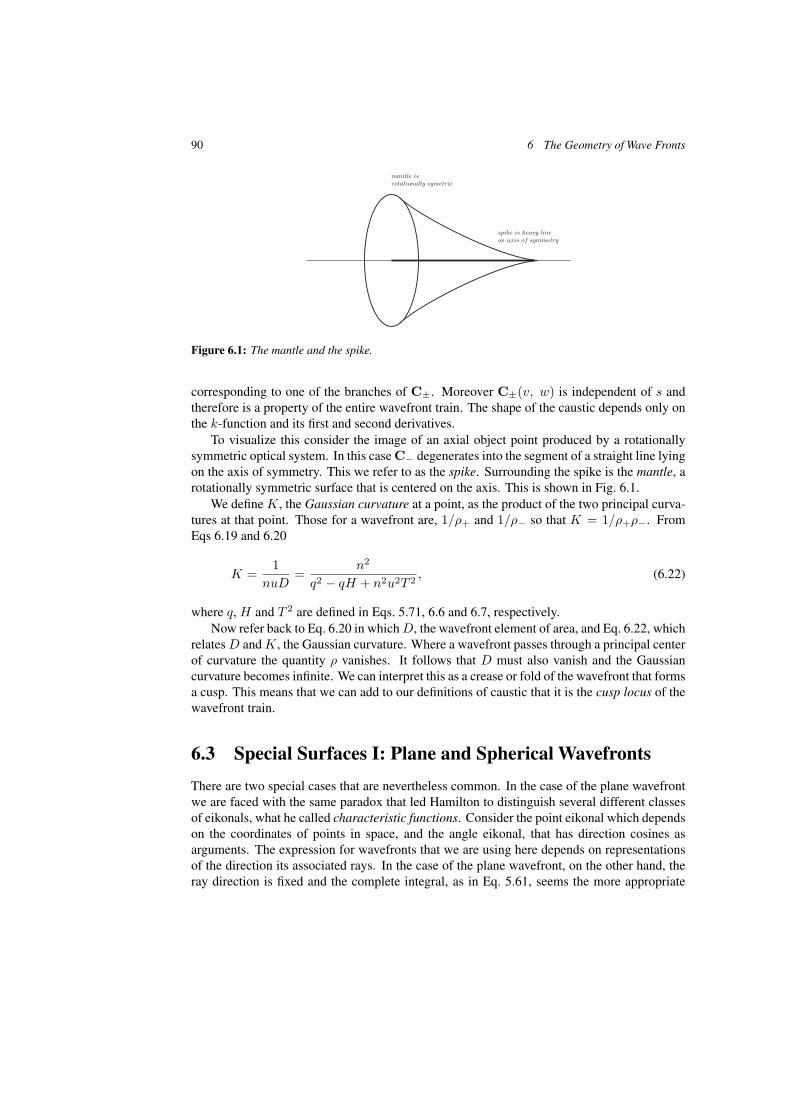
90 6 The Geometry of Wave Fronts
Figure 6.1: The mantle and the spike.
corresponding to one of the branches of C±. Moreover C±(v, w) is independent of s andtherefore is a property of the entire wavefront train. The shape of the caustic depends only onthe k-function and its first and second derivatives.
To visualize this consider the image of an axial object point produced by a rotationallysymmetric optical system. In this case C− degenerates into the segment of a straight line lyingon the axis of symmetry. This we refer to as the spike. Surrounding the spike is the mantle, arotationally symmetric surface that is centered on the axis. This is shown in Fig. 6.1.
We define K, the Gaussian curvature at a point, as the product of the two principal curva-tures at that point. Those for a wavefront are, 1/ρ+ and 1/ρ− so that K = 1/ρ+ρ−. FromEqs 6.19 and 6.20
K =1
nuD=
n2
q2 − qH + n2u2T 2 , (6.22)
where q, H and T 2 are defined in Eqs. 5.71, 6.6 and 6.7, respectively.Now refer back to Eq. 6.20 in which D, the wavefront element of area, and Eq. 6.22, which
relates D and K, the Gaussian curvature. Where a wavefront passes through a principal centerof curvature the quantity ρ vanishes. It follows that D must also vanish and the Gaussiancurvature becomes infinite. We can interpret this as a crease or fold of the wavefront that formsa cusp. This means that we can add to our definitions of caustic that it is the cusp locus of thewavefront train.
6.3 Special Surfaces I: Plane and Spherical Wavefronts
There are two special cases that are nevertheless common. In the case of the plane wavefrontwe are faced with the same paradox that led Hamilton to distinguish several different classesof eikonals, what he called characteristic functions. Consider the point eikonal which dependson the coordinates of points in space, and the angle eikonal, that has direction cosines asarguments. The expression for wavefronts that we are using here depends on representationsof the direction its associated rays. In the case of the plane wavefront, on the other hand, theray direction is fixed and the complete integral, as in Eq. 5.61, seems the more appropriate
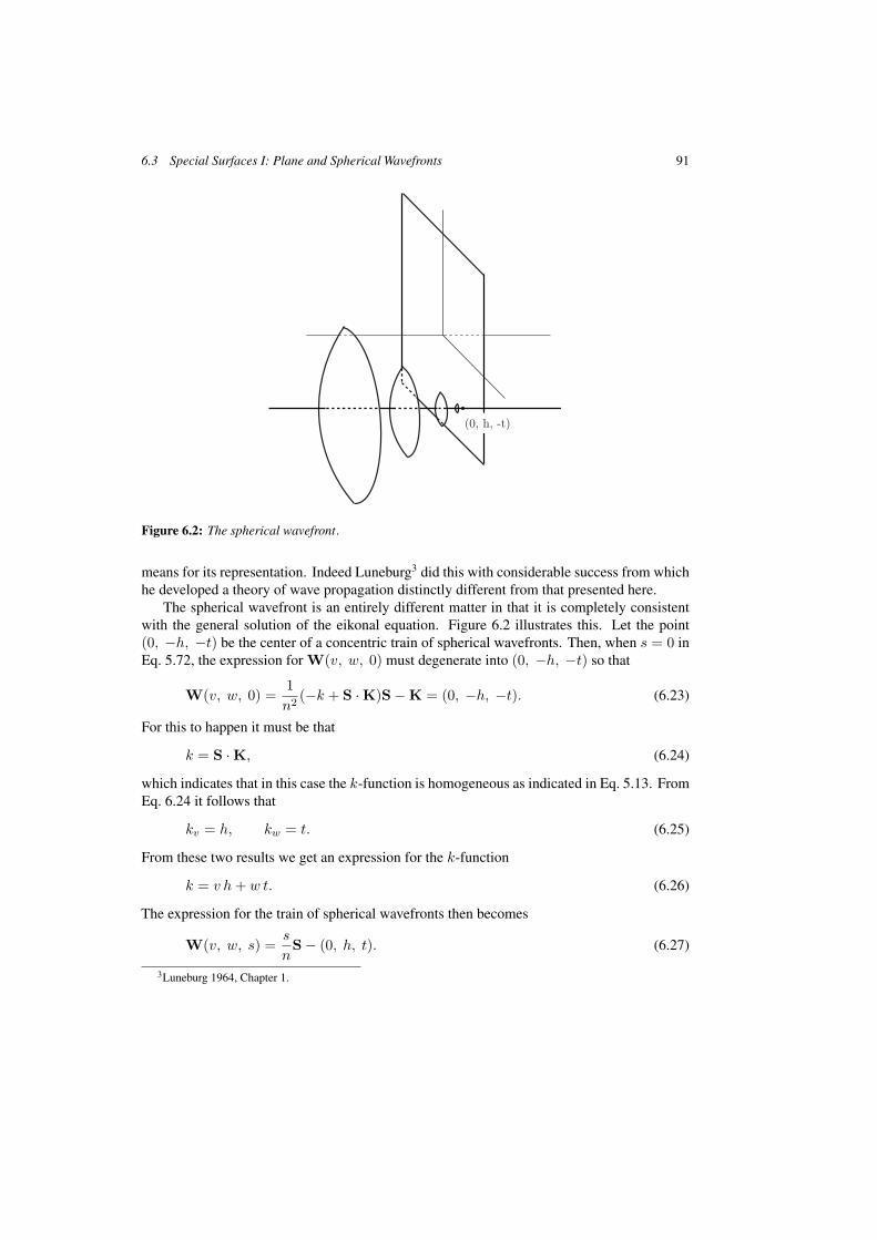
6.3 Special Surfaces I: Plane and Spherical Wavefronts 91
Figure 6.2: The spherical wavefront.
means for its representation. Indeed Luneburg3 did this with considerable success from whichhe developed a theory of wave propagation distinctly different from that presented here.
The spherical wavefront is an entirely different matter in that it is completely consistentwith the general solution of the eikonal equation. Figure 6.2 illustrates this. Let the point(0, −h, −t) be the center of a concentric train of spherical wavefronts. Then, when s = 0 inEq. 5.72, the expression for W(v, w, 0) must degenerate into (0, −h, −t) so that
W(v, w, 0) =1n2 (−k + S · K)S − K = (0, −h, −t). (6.23)
For this to happen it must be that
k = S · K, (6.24)
which indicates that in this case the k-function is homogeneous as indicated in Eq. 5.13. FromEq. 6.24 it follows that
kv = h, kw = t. (6.25)
From these two results we get an expression for the k-function
k = v h + w t. (6.26)
The expression for the train of spherical wavefronts then becomes
W(v, w, s) =s
nS − (0, h, t). (6.27)
3Luneburg 1964, Chapter 1.
92 6 The Geometry of Wave Fronts
To get the derivatives of W we must use Eq. 6.2 which yields
Wv = − s
n u(S × Z), Ww =
s
n u(S × Y). (6.28)
To get D we first calculate
Wv × Ww = − s2
n2u2 (S × Z) × (S × Y)
= − s2
n2u2 [S · (Z × Y)]S
=s2
n2u2 (S · X)S
=s2
n2uS.
(6.29)
Then
D2 = (Wv × Ww)2 =s4
n2u2 ,
so that
D =s2
n u. (6.30)
We will return to the spherical wavefront in Chapter 9.
6.4 Parameter Transformations
As we have stressed repeatedly in previous chapters the transformation of the surface parametersdoes not in any way effect the geometry of a surface;
We introduce two new parameters, p and q, into the vector function for the wavefront Wjust as we had done in Chapter 4
(4.42) P(p, q) = P(v(p, q), w(p, q)
).
By substituting W for P for the derivatives of Eq. 4.43 we get{Wp = Wv vp + Ww wp
Wq = Wv vq + Ww wq.(6.31)
In what follows lower case letters will indicate the first and second fundamental quantitiesassociated with the parameters p and q. The first fundamental quantities are calculated fromChapter 4
(4.45)
e = E v2p + 2F vp wp + Gw2
p
f = E vp vq + F (vp wq + vq wp) + Gwp wq
g = E v2q + 2F vq wq + Gw2
q .
6.4 Parameter Transformations 93
In exactly the same way we calculate the second fundamental quantities. Again referringback to Chapter 4, in particular to,
(4.52)
l = L v2p + 2M vp wp + Nw2
p
m = L vp vq + M(vp wq + vq wp) + N wp wq
n = Lv2q + 2M vq wq + N w2
q .
In terms of the fundamental quantities for the new parameters, p and q, the principalcurvatures are
1ρ±
=l + λ±m
e + λ±f=
m + λ±n
f + λ±g, (6.32)
this from Eqs. 4.18 or 4.25. Here λ is a solution of the quadratic polynomial
(em − fl) + (en − gl)λ + (fn − gm)λ2 = 0, (6.33)
from Eq. 4.19, whose solution is
λ± =−(en − gl) ± R
2(fn − gm). (6.34)
This comes from Eq. 4.20; R, the discriminant of the quadratic equation in Eq. 6.33, is definedin Eq. 4.21 as
R = (en − gl)2 − 4(em − fl)(fn − gm). (6.35)
An alternative expression for λ± is
λ± =−2(em − fl)(en − gl) ± R . (6.36)
From Eqs. 4.22 and 4.23 the two orthogonal principal directions are given by the unit vectors
t± =Wp + λ±Wq√e + fλ± + gλ2±
. (6.37)
Suppose next that the p and q directions are the principal directions. Then Wp and Wq
are vectors tangent to the two orthogonal geodesic curves in the principal directions. It followsthat f = 0, because the two directions are orthogonal, and that m = 0 since they are principaldirections. From Eqs. 4.47 and 4.53{
Evpvq + F (vpwq + vqwp) + Gwpwq = 0
Lvpvq + M(vpwq + vqwp) + Nwpwq = 0.(6.38)
If we make the substitutions wp = λpvp and wq = λqvq, just as we had done in Chapter 4,this becomes{
E + F (λp + λq) + Gλpλq = 0
L + M(λp + λq) + Nλpλq = 0.(6.39)
94 6 The Geometry of Wave Fronts
Now we make the identification λp = λ+ and λq = λ− where λ+ and λ− are solutions of thequadratic polynomial equation in Eq. 4.19. Their sum and product from one of Gauss’ manytheorems, given in Eq. 4.23, satisfy both equations of Eq. 6.39.
As in Chapter 4 when f = m = 0 the polynomial in Eq. 6.33 becomes ephemeral and wecan take as the two roots λp = 0 and λq = ∞. We can justify this by noting that, in generalen − gl �= 0 (an exception to this will be discussed below) so that neither en − gl + R nor(en − gl) − R vanish. On the other hand fl − em ≡ 0. Now refer to Eq. 6.34, in which wecan see that λq = ∞, and to Eq. 6.36 which yields λp = 0.
The remaining two equations in Eq. 4.45 become{e = v2
p(E + 2Fλp + Gλ2p)
g = v2q (E + 2Fλq + Gλ2
q);(6.40)
those from Eq. 4.52 are{l = v2
p(L + 2Mλp + Nλ2p)
n = v2q (L + 2Mλq + Nλ2
q).(6.41)
Now from Eq. 6.32 we can see that the two principal curvatures are
1ρp
=l
e,
1ρq
=n
g(6.42)
just as they should be.Now we can return to the question of the case when en − gl = 0. This happens if and
only if the two curvatures are equal in which case there are no principal directions and all threecoefficients of the quadratic polynomial equation that defines the principal directions are zero.Such a point is called an umbilical point.
6.5 Asymptotic Curves and Isotropic Directions
In Chapter 4 we mentioned two features of geometric surfaces, asymptotic curves and isotropicdirections. Asymptotic directions, as in the case of any direction on a surface, is given by theexpression for the unit tangent vector, Eq. 4.14, where in this case λ is the solution of
L + 2Mλ + Nλ2 = 0, (6.43)
this from Eq. 4.12. If Eq. 6.43 has a real solution then, according to Eq. 4.15, the curvature ofa geodesic curve in the asymptotic directions must vanish. The asymptotic curves then mustbe straight lines.
By substituting the second fundamental quantities from Eq. 6.11 this becomes
[n2u2kvv − q(u2 + v2)]+ 2[n2u2kvw − qvw]λ (6.44)
+ [n2u2kww − q(u2 + w2)]λ2 = 0.

6.5 Asymptotic Curves and Isotropic Directions 95
The discriminant of this quadratic polynomial equation is
∆2 = [n2u2kvw−qvw]2
−[n2u2kvv−q(u2+v2)][n2u2kww−q(u2+w2)]
= −{n4u4(kvvkww − k2vw)
−qn2u2[kvv(n2 − v2) + kww(n2 − w2) − 2vwkvw]
+q2[u4 + u2(v2 + w2)]}= −n2u2[q2 − qH + n2u2T 2],
(6.45)
where we have used Eqs. 6.6 and 6.7.For λ to be real the discriminant must be positive so that
q2 − Hq + n2u2T 2 = n3uD = n2ρ+ρ− ≤ 0. (6.46)
so that ρ+ and ρ− must have opposite signs. This means that the wavefront must lie in a regionwhere it has a saddle point. For this to happen the wavefront must lie between the two causticsheets which implies that these two branches of the caustic must be disjoint. This can be seenin what follows.
The values of q for which asymptotic directions exist are determined by the inequality inEq. 6.46. The boundaries for these values must be the two solutions of the equation obtainedby replacing the inequality by an equal sign thus
q2 − Hq + n2u2T 2 = 0
where the discriminant is H2 − 4n2u2T 2 = S2 from Eq. 6.15 so that the two values of q± are
q± =12(H ± S) (6.47)
But q = ns − k + S · K so that the bounds of s are
s± =1n
[k − (S · K) +
12(H ± S)
](6.48)
From Eq. 6.21 we can calculate
C± · S =12(H ± S) − (S · K)
from which we can get
s± =1n
(k + C± · S). (6.49)
The bounds of s, s±, are functions of v and w.When we substitute the two values, q± into the expression for the wavefronts given in
Eq. 5.72 we get
W± =1
2n2 (H ± S)S − K = C± (6.50)

96 6 The Geometry of Wave Fronts
which shows that the boundary surfaces for the region in which asymptotic directions exist isexactly the two sheets of the caustic surface. The two sheets must therefore be disjoint whichimplies that H must vanish and that T 2 be negative.
What all of this means is that a condition of the existence of asymptotic curves on awavefront is that
H = (n2 − v2)kvv + (n2 − w2)kww − 2vwkvw = 0, (6.51)
a partial differential equation of the second order. This we will return to in Chapter 8, Aberra-tions in Finite Terms.
The isotropic directions are treated in a similar way. Here the defining equation is
E + 2Fλ + Gλ2 = 0, (6.52)
which becomes, after substitution from Eq. 6.5
[(q2 − n2u2T 2)(n2 − w2) + n2u2(H − 2q)kvv]
+[(q2 − n2u2T 2)vw + n2u2(H − 2q)kvw]λ
+[(q2 − n2u2T 2)(n2 − v2) + n2u2(H − 2q)kww]λ2 = 0
(6.53)
whose discriminant is far more difficult to calculate and far less rewarding.
∆2 = [(q2 − n2u2T 2)vw + n2u2(H − 2q)kvw]2
−[(q2 − n2u2T 2)(n2 − w2) + n2u2(H − 2q)kvv]
×[(q2 − n2u2T 2)(n2 − v2) + n2u2(H − 2q)kww]
= −n2u2{(q2 − n2u2T 2)2 + H(q2 − n2u2T 2)(H − 2q)
+n2u2T 2(H − 2q)2}= −n2u2(q2 − Hq + n2u2T 2)2,
(6.54)
This quantity can never be positive so that there are no real solutions for λ. This indicates thatthere can be no isotropic directions for wavefronts.
This concludes this chapter on wavefronts. In it we have found the principal directions andprincipal curvatures of each wavefront in a wavefront train as well as its caustic surface. We de-rived expressions for transforming the wavefront parameters. We also looked at the possibilityof there being asymptotic curves imbedded on the wavefront. We also found that wavefrontscan have no isotropic directions. We examined two special cases, the plane wavefront and thetrain of spherical wavefronts. These items will be treated further in subsequent chapters.
At this point it should be evident that the k-function and its derivatives determine completelythe structure of the individual wavefronts in a train and the associated caustic surface.
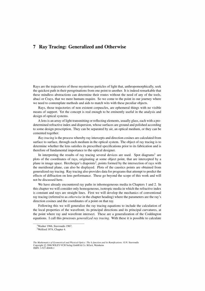
The Mathematics of Geometrical and Physical Optics: The k-function and its Ramifications. O.N. StavroudisCopyright c© 2006 WILEY-VCH Verlag GmbH & Co. KGaA, WeinheimISBN: 3-527-40448-1
7 Ray Tracing: Generalized and Otherwise
Rays are the trajectories of those mysterious particles of light that, anthropomorphically, seekthe quickest path in their peregrinations from one point to another. It is indeed remarkable thatthese mindless abstractions can determine their routes without the need of any of the tools,abaci or Crays, that we mere humans require. So we come to the point in our journey wherewe need to contemplate methods and aids to match wits with these peculiar objects.
Rays, those trajectories of non existent corpuscles, are ephemeral things with no visiblemeans of support. Yet the concept is real enough to be eminently useful in the analysis anddesign of optical systems.
A lens is an array of light transmitting or reflecting elements, usually glass, each with a pre-determined refractive index and dispersion, whose surfaces are ground and polished accordingto some design prescription. They can be separated by air, an optical medium, or they can becemented together.
Ray tracing is the process whereby ray intercepts and direction cosines are calculated fromsurface to surface, through each medium in the optical system. The object of ray tracing is todetermine whether the lens satisfies its prescribed specifications prior to its fabrication and istherefore of fundamental importance to the optical designer.
In interpreting the results of ray tracing several devices are used. Spot diagrams1 areplots of the coordinates of rays, originating at some object point, that are intercepted by aplane in image space. Herzberger’s diapoints2, points formed by the intersection of rays withthe meridional plane, can also be displayed. Plots of the caustics points are obtained fromgeneralized ray tracing. Ray tracing also provides data for programs that attempt to predict theeffects of diffraction on lens performance. These go beyond the scope of this work and willnot be discussed here.
We have already encountered ray paths in inhomogeneous media in Chapters 1 and 2. Inthis chapter we will consider only homogeneous, isotropic media in which the refractive indexis constant and rays are straight lines. First we will develop the mechanics of conventionalray tracing (referred to as otherwise in the chapter heading) where the parameters are the ray’sdirection cosines and the coordinates of a point on that ray.
Following this we will generalize the ray tracing equations to include the calculation ofthe local properties of the wavefront; its principal directions and its principal curvatures, atthe point where ray and wavefront intersect. These are a generalization of the Coddingtonequations. I call this processes generalized ray tracing. With these it is possible to calculate
1Washer 1966, Stavroudis 1967.2Welford 1974, Chapter 4.
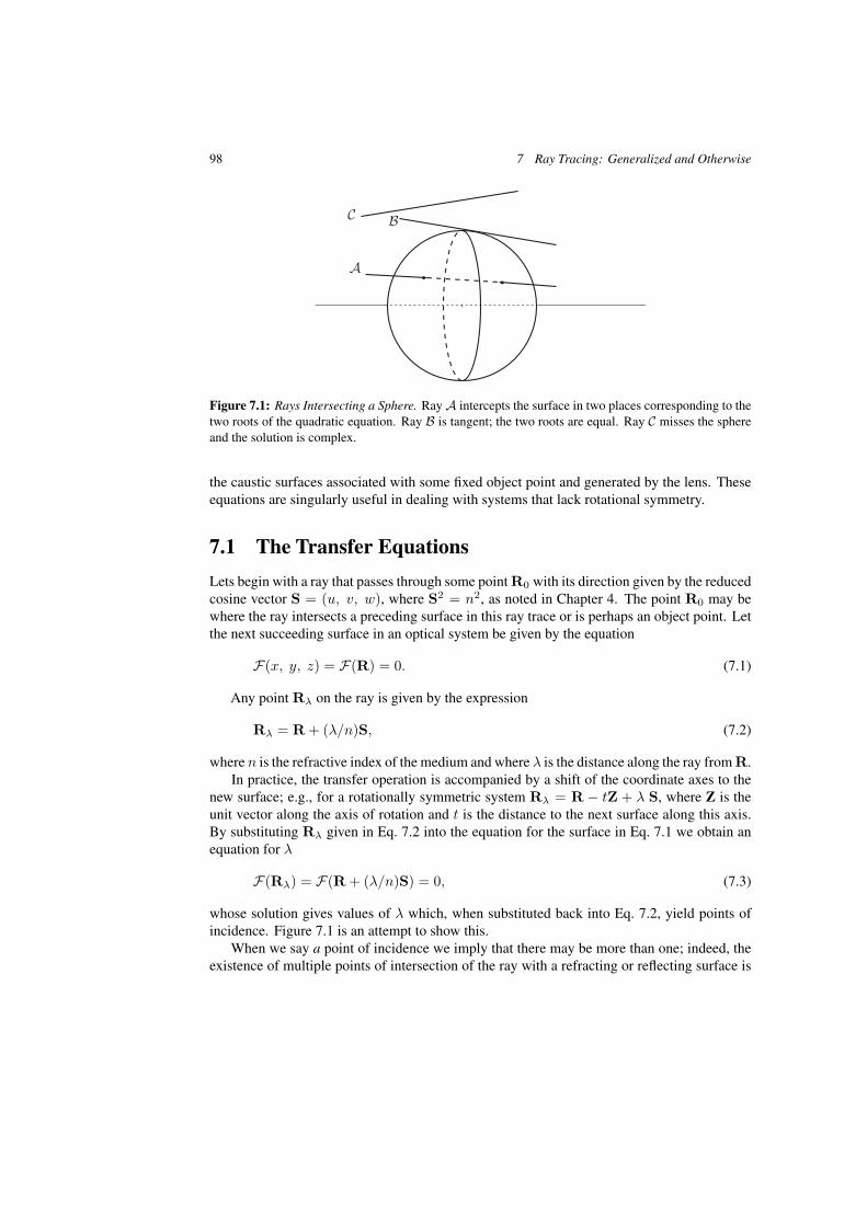
98 7 Ray Tracing: Generalized and Otherwise
Figure 7.1: Rays Intersecting a Sphere. Ray A intercepts the surface in two places corresponding to thetwo roots of the quadratic equation. Ray B is tangent; the two roots are equal. Ray C misses the sphereand the solution is complex.
the caustic surfaces associated with some fixed object point and generated by the lens. Theseequations are singularly useful in dealing with systems that lack rotational symmetry.
7.1 The Transfer Equations
Lets begin with a ray that passes through some point R0 with its direction given by the reducedcosine vector S = (u, v, w), where S2 = n2, as noted in Chapter 4. The point R0 may bewhere the ray intersects a preceding surface in this ray trace or is perhaps an object point. Letthe next succeeding surface in an optical system be given by the equation
F(x, y, z) = F(R) = 0. (7.1)
Any point Rλ on the ray is given by the expression
Rλ = R + (λ/n)S, (7.2)
where n is the refractive index of the medium and where λ is the distance along the ray from R.In practice, the transfer operation is accompanied by a shift of the coordinate axes to the
new surface; e.g., for a rotationally symmetric system Rλ = R − tZ + λ S, where Z is theunit vector along the axis of rotation and t is the distance to the next surface along this axis.By substituting Rλ given in Eq. 7.2 into the equation for the surface in Eq. 7.1 we obtain anequation for λ
F(Rλ) = F(R + (λ/n)S) = 0, (7.3)
whose solution gives values of λ which, when substituted back into Eq. 7.2, yield points ofincidence. Figure 7.1 is an attempt to show this.
When we say a point of incidence we imply that there may be more than one; indeed, theexistence of multiple points of intersection of the ray with a refracting or reflecting surface is
7.1 The Transfer Equations 99
Figure 7.2: The Local Coordinate System. The origin is placed at the vertex of the rotationally symmetricrefracting surface – the point where the lens axis intersects the surface.
one of the annoying difficulties in developing formulas for the transfer operation, particularlyfor systems that lack rotational symmetry. The commonest refracting surface is the sphere, aquadratic surface where the function F is a polynomial of the second degree. The equationcorresponding to Eq. 7.3 will have two roots that identify the two points of intersection of astraight line with that sphere. If these roots are equal then the ray is tangent to the refractingsphere; if they are complex then the ray has no real point of intersection and misses the surface.What is said here applies to any quadratic surface and therefore includes conic surfaces suchas prolate spheroids, oblate spheroids, paraboloids and hyperboloids of one and two sheets.
In rotationally symmetric systems, the local coordinate origin is taken to be at the inter-section of the system’s axis of symmetry with the refracting conic surface, usually referred toas the vertex, and is shown in Fig. 7.2. The point of incidence is that branch of the quadraticsolution nearest the origin. This way of avoiding decision making fails for systems that are offaxis or not rotationally symmetric, especially when the details of the ray tracing calculations areobscured by the arcana of a computer program. This problem will be discussed in Chapter 11that deals with the modern schiefspiegler, a wildly off-axis reflecting optical system.
The transfer operation does more than find the points of incidence but includes the calcu-lation of other quantities as well. The most important of these is the unit normal vector of therefracting surface at the point of incidence that we encountered in Chapter 4
(4.98) N =∇F√(∇F)2
.
For generalized ray tracing, the principal directions and the principal curvatures of the wavefrontat the point of intersection of ray and wavefront will also be required.
100 7 Ray Tracing: Generalized and Otherwise
7.2 The Ancillary Quantities
The details of calculating N come next. The equation in Eq. 7.1 defines z as an implicitfunction of x and y so that its partial derivatives become
∂F∂x
+∂F∂z
∂z
∂x= 0,
∂F∂y
+∂F∂z
∂z
∂y= 0. (7.4)
The gradient then becomes
∇F =(
∂F∂x
,∂F∂y
,∂F∂z
)= −∂F
∂z
(∂z
∂x,
∂z
∂y,−1
). (7.5)
We will also need to calculate the surface parameters of the refracting surface at the point ofincidence, the principal directions and curvatures, that are required for generalized ray tracing.
In Chapter 4 we saw that a surface can be represented as a vector function of two parametersand that those two parameters can be the x and y coordinates of a point on a plane. Then thevector function can be written as
(4.90) R(x, y) =(x, y, z(x, y)
),
so that the partial derivatives are
(4.91) Rx = (1, 0, zx) Ry = (0, 1, zy),
from which we can calculate the unit normal vector
(4.93) N = − (zx, zy, −1)√1 + z2
x + z2y
and the first fundamental quantities from Eq. 4.4
E = 1 + z2x, F = zxzy, G = 1 + z2
y . (7.6)
Also using Eq. 4.11 we can calculate the second fundamental quantities
L =zxx√
1 + z2x + z2
y
M =zxy√
1 + z2x + z2
y
N =zyy√
1 + z2x + z2
y
. (7.7)
From Eqs. 7.6 and 7.7, using Eqs. 4.18, 4.19, 4.21 and 4.25, the principal directions andprincipal curvatures of the refracting surfaces at the point of incidence can be calculated.These quantities will be needed when we come to generalized ray tracing later in this chapter.
7.3 The Refraction Equations
In Chapter 3 we derived the two versions of Snell’s law, the vector form
(3.51) S1×N = S×N,
7.3 The Refraction Equations 101
and the scalar form
(3.49) n1 sin r = n sin i,
where i stands for the angle of incidence, the angle between the surface normal and the incidentray, and r, the angle of refraction, the angle between the surface normal and the refracted ray,as discussed in Chapter 4.
The two reduced ray vectors are S for the incident ray and S1 for the refracted ray so thatn cos i = S · N and n1 cos r = S1 · N where N is the unit vector normal to the refractingsurface at the point of incidence as in Eq. 4.93.
Now we rearrange the vector form of Snell’s law, Eq. 3.51, as follows:
(S1 − S) × N = 0, (7.8)
which shows that the vector S1 −S must be parallel to N. Then there must exist some quantityγ so that S1 − S = γN whence comes
S1 = S + γN, (7.9)
the refraction equation. By taking the scalar product of this with N we get
γ = S1 · N − S · N = n1 cos r − n cos i. (7.10)
The formula for reflection is highly artificial. In the usual convention one sets n1 = −n(n = 1 in air) in Eqs. 7.9 and 7.10. Since sin r = − sin i it must be that cos r = cos i so that,γ = −2 cos i and,
S1 = −S + 2 cos iN. (7.11)
So with the two equations, Eqs. 7.9 and 7.10, we are able to find the refracted ray vectorS1 when the incident ray vector S, the surface normal N and refractive indices n and n1 areknown. Equation 3.49, the scalar version of Snell’s law, is used to find sin r from sin i and thetwo refractive indices.
From Eq. 7.9 it is clear that S1 is a linear combination of N and S. The three vectors arethen coplanar; the plane so determined is called the plane of incidence.
This completes this section on ordinary ray tracing. With the formulas derived here onecan trace a system of rays through an optical system to some plane in image space wherethe ray intercepts can be plotted. The result is a spot diagram3 (once called a focal plot inthe ancient literature) that can illustrate quite graphically the distribution of the light on someplane in image space. With ray tracing, graphs can be plotted of the point coordinates in imagespace versus coordinates on an entrance pupil to reveal details of the aberrations associatedwith a particular object point. When image point coordinates are plotted versus object pointcoordinates the data will show distortion and image curvature.4 These are details that we willnot delve into here.
3Stavroudis and Sutton 1965.4Stavroudis, 1972a, Chapter XII.

102 7 Ray Tracing: Generalized and Otherwise
One needs to add to all this that the spot diagram is the geometric analog of the starimage test in which collimated light is made to enter the lens under test. The quality of theimage formed and the distribution of the light in that image provides measures of the lensesperformance. Because of this, the spot diagram is able to indicate how a lens will behavebefore its fabrication.5
But there is a limitation. We speak of geometric aberrations. When these are large theydominate image formation. But if they are sufficiently small, diffraction effects dominate andgeometry has little or no influence of the formation of an image. Such a situation is commonlyreferred to as being diffraction limited.6
7.4 Rotational Symmetry
By far most optical systems are rotationally symmetric; each surface in such a system mustitself be rotationally symmetric and then all of the lines of symmetry of the component surfacesmust coincide, thus forming an axis of symmetry for the entire system.
As a matter of convenience we will use a coordinate system in which the z-axis is placed onthe axis of symmetry and a local coordinate origin is located where this axis and the refractingsurface intersect. This point is usually referred to as the vertex.
In a rotationally symmetric system the axis of symmetry and an object point determinea plane, the meridional plane. Rays on this plane are called meridional rays; rays that arenot meridional rays are called skew rays, thus distinguishing two disjoint classes of rays.Meridional rays remain meridional rays as they progress through a rotationally symmetricoptical system; skew rays can never become meridional rays. Of course, this distinctiondoesn’t apply to off-axis systems.
In rotationally symmetric systems diapoints7 can be calculated using the ray tracing equa-tions; these are the points of intersection of skew rays on a meridional plane and are usefulin visualizing the geometric aberrations of a lens. Diapoints and their uses will be discussedfurther in Chapter 8, Aberrations in Finite Terms.
One additional point. If an optical system is rotationally symmetric then there is a quantitycalled skewness that is an invariant under both refraction and transfer. If the axis of symmetryis the z-axis, if P = (x, y, z) is any point on a skew ray with a direction cosine vector isS = (ξ, η, ζ) then skewness is given by8
K = n(xη − yξ) = nZ · (P × S). (7.12)
The skewness K is a measure of the angle a skew ray makes with the meridional plane; itvanishes for meridional rays. That it is indeed invariant can be verified from Eqs. 7.2 and 7.9.
5Stavroudis 1972a, pp. 228 et seq.6Born and Wolf 1998, Chapter XII.7Herzberger 1958, Chapter 7.8Stavroudis 1972a, pp. 208–209.
7.5 The Paraxial Approximation 103
7.5 The Paraxial Approximation
In rotationally symmetric systems it is common to construct linear approximations of the raytracing equation in which all points are assumed to lie arbitrarily near the axis of symmetry.All quantities of quadratic degree and higher are small and are assumed to be zero. Thisneighborhood of the axis is referred to as the paraxial region; the resulting approximationsare called the paraxial ray tracing equations. Ray traced with these approximate formulas arecalled paraxial rays even if their coordinates lie far outside the paraxial region.9
In what follows each surface is rotationally symmetric and is expressed in terms of acoordinate system whose origin is at its vertex, the point where the surface and its axis intersect.A power series expansion for z defines the surface,
z =∞∑
n=0
an(x2 + y2)n
so that its two first partial derivatives are
zx = 2a1x + 2x
∞∑n=2
nan(x2 + y2)n−1
zy = 2a1y + 2y
∞∑n=2
nan(x2 + y2)n−1.
Now referring to Eq. 4.93, in the paraxial approximation, ignoring all terms of degree greaterthan one the unit normal vector to the refracting surface becomes
N = (x, y, 1). (7.13)
The sine and cosine functions can also be represented as power series;
sin u = u +∞∑
n=1
(−1)n
(2n + 1)!u2n+1 cos u = 1 +
∞∑n=1
(−1)n
(2n)!u2n
so that, in the paraxial approximation, sin u = u and cos u = 1. The paraxial approximationof the scalar form of Snell’s law, Eq. 3.49, becomes
n1i1 = n i, (7.14)
Where i and i1 are the paraxial angles of incidence and refraction. The refraction equation,Eqs. 7.9 and 7.10 degenerates to
n1u1 = nu + c h(n1 − n), (7.15)
where c is the curvature of the refracting sphere and h is the height of the paraxial ray on thereflecting sphere. I won’t attempt to explain how the paraxial approximation of a sphere is aplane and at the same time have a curvature.
9Stavroudis 2001, pp. 22–28.

104 7 Ray Tracing: Generalized and Otherwise
The transfer equation, Eq. 7.2 becomes
h1 = h + tu (7.16)
where t is the distance along the axis of symmetry between the two surfaces, h is the paraxialray hight on the initial surface and h1 is its counterpart on the second surface.
The skewness invariant, given in Eq. 7.12 is a quadratic quantity and therefore vanishesunder the paraxial approximation. This implies that paraxial rays cannot be skew rays; that allparaxial rays throughout an optical system must lie on a meridional plane.
The Lagrange invariant L10 is defined by
L = n(yu − yu) = n1(y1u1 − y1u1) (7.17)
where y, u and y, u are two paraxial rays. If L �= 0 the two rays are said to be independent.If we think of paraxial rays as vectors on the meridian plane, since this plane is two-
dimensional, then all paraxial rays can be written as a linear combination of only two vectorsthat can serve as a basis for a vector space consisting of the totality of the paraxial rays. Thetwo base vectors must be independent; this is assured by the non vanishing of the Lagrangianinvariant.
Suppose the two basis rays are h, for height, and u, for slope and h and u; if the Lagrangeinvariant, does not vanish then these two rays are independent and can act as basis elements.The choice of these rays is entirely arbitrary; any pair of paraxial rays for which L �= 0 willdo.
It is convenient to choose these basis rays to be the paraxial marginal ray, that ray that justclears the edges of all elements in an optical system, and the paraxial chief ray, the ray thatpasses through the center of the dominant aperture.11
These rays are fundamental to the calculation of the Seidel and higher order aberrations ofa lens. This will not be discussed here.
7.6 Generalized Ray Tracing – Transfer
Generalized Ray Tracing12 (generalized Coddington Equations might be a more accurate term)is the subject of these next sections. We are already accustomed to using the vector functionof three components W(v, w, s) to represent a wavefront train as well as the use of N asthe unit normal vector. To simplify our calculations assume that the parametric curves of thewavefronts are in the principle directions. In Chapter 4, using Eqs. 4.67 through 4.70, wesaw that we could always make such a transformation of parameters. Take two positions of awavefront corresponding to s and s + λ. Then
W(v, w, s + λ) = W(v, w, s) + λN(v, w, s),
or, to simplify matters
Wλ = W + λN.10Stavroudis 1972a, pp. 209–210.11Welford 1974, pp. 22–25.12Stavroudis and Sutton, 1965.
7.7 Generalized Ray Tracing – Preliminary Calculations 105
Taking derivatives we get{Wλ
v = Wv + λNv = [1 − λ (L/E)]Wv
Wλw = Ww + λNw = [1 − λ (N/G)]Wv
(7.18)
where we have used the Weingarten equations from Eq. 4.35. Here F = 0 and M = 0 becauseof our assumption that the lines of curvature were in the principal directions. These lead to thefirst fundamental quantities
Eλ = [1 − λ (L/E)]2 E Gλ = [1 − λ (N/G)]2 G, (7.19)
and to the second fundamental quantities
Lλ = [1 − λ (L/E)]L Nλ = [1 − λ (N/G)] N, (7.20)
obtained by again using the Weingarten equations. Next we use Eqs. 4.37 and 4.40 to calculatethe principal curvatures
1ρλ
v
=Lλ
Eλ=
1ρv − λ
1ρλ
w
=Nλ
Gλ=
1ρw − λ
. (7.21)
This tells us that the wavefront principal centers of curvature do not change as the wavefrontprogresses. We also can show that the principal directions do not change on transfer.
7.7 Generalized Ray Tracing – Preliminary Calculations
Recall that the plane of incidence is determined by the surface normal, N, and the incident rayvector S and that as a consequence of Snell’s law, Eq. 3.49, the refracted ray vector S1 alsolies on this plane. We define the unit vector P to be perpendicular to the plane of incidenceand use the ratio of the two expressions in Eqs. 3.49 and 3.51 to obtain
P =S1 × Nn sin r
=S × Nn1 sin i
. (7.22)
To show that these vectors are indeed equal both the vector form and the scalar form of Snell’slaw are used.
Next we define the vector Q for the incident wavefront, Q for the refracting surface, andQ1 for the refracted wavefront as follows
Q = (S × P)/n, Q = N × P, Q1 = (S1 × P)/n1, (7.23)
which leads to the following vector relationships
P = (Q × S)/n, P = Q × N, P = (Q1 × S1)/n1,
S = n(P × Q), N = P × Q, S1 = n1(P × Q1).(7.24)
106 7 Ray Tracing: Generalized and Otherwise
It follows from the definition of the Q vectors in Eq. 7.23 and the refraction equation inEq. 7.9 that
n1Q1 = nQ + γQ, (7.25)
where γ is defined in Eq. 7.10. As a result of the transfer operations we have the point ofincidence P, the two principal curvatures of the wavefront at P, 1/ρξ and 1/ρη, and one ofthe principal directions which we refer to as T.
On the refracting surface at the point of incidence R, we do the same calculations and getthe unit normal vector N, the two principal curvatures 1/ρξ and 1/ρη, and one of the principaldirections T.
For the incident wavefront we find the angle between the wavefront principal directionand P
cos θ = T · P. (7.26)
Using Eq. 4.66 derived in Chapter 4 we find the curvatures of the geodesics tangent to P andQ and the torsion 1/σ
1ρp
=cos2 θ
ρξ+
sin2 θ
ρη
1ρq
=sin2 θ
ρξ+
cos2 θ
ρη
1σ =
(1ρξ
− 1ρη
)sin θ cos θ.
(7.27)
We make the same calculations for the refracting surface. First the angle between a principaldirection of the refracting surface and P
cos θ = T · P, (7.28)
then the curvatures of the geodesics tangent to P and Q and the torsion of the curve 1/σ
1ρp
=cos2 θ
ρξ
+sin2 θ
ρη
1ρq
=sin2 θ
ρξ
+cos2 θ
ρη
1σ
=(
1ρξ
− 1ρη
)sin θ cos θ,
(7.29)
exactly as was done in Eq. 4.66.Recall the Frenet-Serret equations and the relations between t, n and b from Chapter 2
(2.10) t = n×b, n = b×t, b = t×n,
7.7 Generalized Ray Tracing – Preliminary Calculations 107
and
(2.20)
(t · ∇)t =1ρn
(t · ∇)n = −1ρt +
1τb
(t · ∇)b = −1τn
where we have used directional derivatives.For the geodesic curve tangent to P we make the following identifications:
tp = P
np = S/n
bp = tp × np = (P × S)/n = −Q
(7.30)
where we have made use of Eqs. 7.23 and 7.24.Applying these relations to the Frenet-Serret equations given in Eq. 2.12, results in
(2.12)
(tp · ∇)tp =1
nρpnp
(tp · ∇)np = − n
ρptp +
n
τpbp
(tp · ∇)bp = − 1nτp
np
which becomes, using Eq. 7.30
(P · ∇)P =1
nρpS
(P · ∇)S = − n
ρpP +
n
τpQ
−(P · ∇)Q = − 1nτp
S.
(7.31)
Now for the geodesic curve tangent toQwe make these identifications again using Eqs. 7.23and 7.24
tq = Q
nq = S/n
bq = tq × nq = (Q × S)/n = P.
(7.32)
108 7 Ray Tracing: Generalized and Otherwise
By making the obvious substitutions from Eq. 7.32, as in the previous case we get
(Q · ∇)Q =1
nρqS
(Q · ∇)S = − n
ρqQ +
n
τqP
(Q · ∇)P = − 1nτq
S.
(7.33)
We know from Eq. 4.41 that the two values of torsion are equal in magnitude and oppositein sign so that we may define
1σ
= − 1τp
=1τq
. (7.34)
This results in, for the P geodesic, from Eq. 7.31
(P · ∇)P =1
nρpS
(P · ∇)S = − n
ρpP +
n
σQ
(P · ∇)Q = − 1nσ
S,
(7.35)
and for the Q geodesic, where we use Eq. 7.33
(Q · ∇)Q =1
nρqS
(Q · ∇)S = − n
ρqQ +
n
σP
(P · ∇)P = − 1nσ
S.
(7.36)
Since S and Q, N and Q, S1 and Q1 are all coplanar, we may also write
S = N cos i + Q sin i, S1 = N cos r + Q sin r,
Q = −N sin i + Q cos i, Q1 = −N sin r + Q cos r,(7.37)
from which we can get
Q = S sin i + Q cos i = S1 sin r + Q1 cos r. (7.38)
Finally we note that, since rays in homogeneous media are always straight lines
(S · ∇)S = (S1 · ∇)S1 = 0. (7.39)
7.8 Generalized Ray Tracing – Refraction 109
7.8 Generalized Ray Tracing – Refraction
Now we come to the derivation of the equations for generalized ray tracing13. We take thederivative of the vector form of Snell’s law, given in Eq. 3.51, in the direction of P and get
[(P · ∇)S1] ×N + S1 × [(P · ∇)N]
= [(P · ∇)S] × N + S × [(P · ∇)N],(7.40)
The process of evaluating this is long and complicated so we must calculate separately theindividual terms of Eq. 7.40 as follows.
[(P · ∇)S1] × N =(
−n1
ρ′p
P +n1
σ′ Q1
)× N
= −n1
ρ′p
(P × N) +n1
σ′ (−N sin i + Q cos i) × N
= −n1
ρ′p
Q +n1
σ′ P.
(7.41)
Here and in the following calculations we have used Eqs. 7.23, 7.24, 7.35 and 7.38
[(P · ∇)S] × N =(
− n
ρpP +
n
σQ
)× N
= − n
ρp(P × N) +
n
σ(−N sin i + Q cos i) × N
=n
ρpQ +
n
σP.
(7.42)
S1 × [(P · ∇)N] = S1 ×[− 1
ρpP +
1σQ
]
= − 1ρp
S1 × P +n1
σ(N cos r + Q cos r) × Q
= −n1
ρpQ1 − n1 cos r
σP.
(7.43)
S × [(P · ∇)N] = S ×[− 1
ρpP +
1σQ
]
= − 1ρp
S × P +n
σ(N cos i + Q sin i) × Q
= − n
ρpQ − n cos r
σP.
(7.44)
13Stavroudis 1976.
110 7 Ray Tracing: Generalized and Otherwise
Putting these, Eqs. 7.41, 7.42, 7.43 and 7.44, all together yields
n1
ρ′p
Q +n1 cos r
σ′ P − n1 cos r
σP − 1
ρp(nQ + γQ)
=n
ρpQ +
n cos i
σP − n cos i
σP − n
ρpQ.
(7.45)
Collecting terms in P and Q we get
P[n1 cos r
σ′ − n1 cos r
σ− n cos i
σ+
n cos i
σ
]+ Q
[n1
ρ′p
− γ
ρp− n
ρp
]= 0. (7.46)
Since P and Q are orthogonal each of the two coefficients must equal zero independently.This results in
n1ρ′
p=
n
ρp+
γ
ρp
n1 cos rσ′ =
n cos i
σ+
n1 cos r − n cos i
σ
=n cos i
σ+
γ
σ
(7.47)
Now we take the derivative of the vector form of Snell’s law in Eq. 3.50 in the direction ofQ and get
n1{[(Q · ∇)S1] × N + S1 × [(Q · ∇)N]}= n{[(Q · ∇)S] × N + S × [(Q · ∇)N]},
(7.48)
As before we calculate the individual terms. Here we use Eq. 7.39 in addition to Eqs. 7.22,7.23 and 7.36.
(Q · ∇)S1 = [(S1 sin r + Q1 cos r) · ∇]S1
= cos r(Q1 · ∇)S1
= n cos r
[− 1
ρ′q
Q1 +1σ′ P
].
(7.49)
[(Q · ∇)S1] × N = n1 cos r
[−1ρ′
q
Q1 +1σ′ P
]× N
= n1 cos r
[−1ρ′
q
(−N sin r + Q cos r) × N − 1σ′ Q
]
= −n1 cos2 r
ρ′q
P − n1 cos r
σQ.
(7.50)
7.8 Generalized Ray Tracing – Refraction 111
(Q · ∇)S = [(S sin i + Q cos i) · ∇]S
= sin i(S · ∇)S + cos i(Q · ∇)S
= n cos i
[− 1
ρqQ +
1σP
].
(7.51)
[(Q · ∇)S] × N = n cos i
[− 1
ρq(Q × N) +
1σ
(P × N)]
= n cos i
[− 1
ρq(−N sin i + Q cos i) × N − 1
σQ
]
= −n cos2 i
ρqP − n cos i
σQ.
(7.52)
S1 × [(Q · ∇)N] = S1 ×[− 1
ρqQ +
1σQ1
]
= − 1ρq
S1 × (S1 sin r + Q1 cos r) +1σ
(S1 × P)
=n1 cos r
ρqP +
n1
σQ1.
(7.53)
S × [(Q · ∇)N] = S ×[− 1
ρqQ +
1σQ1
]
= − 1ρq
S × (S sin i + Q cos i) +1σ
(S × P)
=n cos i
ρqP +
n
σQ.
(7.54)
Substituting Eqs. 7.50, 7.52, 7.53 and 7.54 back into Eq. 7.48 yields
−n1 cos2 r
ρ′q
P − n1 cos r
σ′ Q +n1 cos r
ρqP +
1σ
(nQ + γQ)
= −n cos i
ρq− n cos i
σQ +
n cos i
ρqP +
n
σQ
(7.55)
Collecting terms in Eq. 7.55, we get
P[−n1 cos2 r
ρ′q
+n1 cos r
ρq+
n cos2 i
ρq− n cos i
ρq
]
+Q[−n1 cos r
σ+
γ
σ+
n cos i
σ
]= 0.
(7.56)
112 7 Ray Tracing: Generalized and Otherwise
As before we set the coefficients equal to zero and get
n1 cos2 r
ρ′q
=n cos2 i
ρq+
n1 cos r − n cos i
ρq
=n cos2 i
ρq+
γ
ρq
n1 cos r
σ=
n cos i
σ+
γ
σ.
(7.57)
Collecting the results of Eqs. 7.47 and 7.57 we obtain
n1 cos2 r
ρ′q
=n cos2 i
ρq+
γ
ρq
n1 cos r
σ′ =n cos i
σ+
γ
σn1
ρ′p
=n
ρp+
γ
ρp.
(7.58)
The first and third of these are the Coddington equations.These now provide us with 1/ρ′
q, 1/σ′ and 1/ρ′p.
By inverting the equations in Eq. 7.27 and applying the result to the refracted wave front,we get
tan 2θ′ =2/σ′
1/ρ′p − 1/ρ′
q
, (7.59)
and
1ρ′
ξ
=cos2 θ′
ρ′p
+sin2 θ′
ρ′q
− sin 2θ′
σ′
1ρ′
η
=sin2 θ′
ρ′p
+cos2 θ′
ρ′q
+sin 2θ′
σ′
(7.60)
which gives us the two principal curvatures of the refracted wave front at the point where rayand wavefront intersect.
One of the principal directions, the vector T′, is given by
T′ = P cos θ′ + Q1 sin θ′. (7.61)
To conclude and recapitulate, ordinary ray tracing consists of two operations, transfer andrefraction. Generalized ray tracing consists of transfer, extended to include the calculation ofprincipal radii of curvature, ordinary refraction, a rotation of component vectors and curvaturesto positions normal to and lying in the plane of incidence. This is followed by an applicationof the augmented Coddington equations as given in Eq. 7.58 followed by another rotation tothe principal directions as in Eqs. 7.59 and 7.60.
7.9 The Caustic 113
7.9 The Caustic
We have derived Eqs. 7.58 through 7.61 that yield formulas for the two principal curvatures1/ρ′
ξ and 1/ρ′η as well as T′, one of the two principal directions; the second comes from the
vector product of T′ and S1. These processes can be iterated from surface to surface throughan optical system. Suppose we start at some fixed object point and trace a ray passing throughthat point through the optical system to image space. The ray trace will terminate at somesurface, the last refracting surface or the exit pupil. At that point there passes a wavefrontwhose principal directions are given by T′ and T′ × S1 and whose two principal curvaturesare 1/ρ′
ξ and 1/ρ′η.
The reciprocals of the principal curvatures, ρ′ξ and ρ′
η, are the two principal radii of cur-vature, the distances to the two principal centers of curvature and therefore are the two pointslying on the caustic surface. The coordinates of the caustic points can be calculated by usingthe transfer equation, Eq. 7.2.
One of the definitions of the caustic surface is that it is the locus of the principal centers ofcurvature and is therefore a surface of two sheets on each of which lies one of the two principalcenters of curvature.
7.10 The Prolate Spheroid
An excellent example of the use of generalized ray tracing is its application to the reflectingprolate spheroid whose equations we encountered in Chapter 4. The point of incidence
(4.75) R = �(sin φ sin θ, sin φ cos θ, cos φ),
where the radius vector � was derived in Chapter 2 as
(2.36) � =r
1 − ε cos φ.
We will also need φ′, the angle opposite φ
(2.38)
{sin φ′ = (1 − ε2) sin φ/K2,
cos φ′ =[2ε − (1 + ε2) cos φ
]/K2,
where
(2.39) K2 = (1+ε2)−2ε cos φ,
as well as �′ the distance between the point on the surface and the distal focus
(2.40) �′ =rK2
(1 − ε2)(1 − ε cos φ)=
� K2
1 − ε2.
There we also obtained the differential element of area
(4.79) D2 = EG−F 2 =�4 sin2 φ
(1 − ε cos φ)2K2,

114 7 Ray Tracing: Generalized and Otherwise
as well as the unit normal vector
(4.81) N =1K
(sin φ sin θ, sin φ cos θ, cos φ−ε
),
and the principal directions given as unit vectors
(4.84)
T+ =1K
((cos φ − ε) sin θ, (cos θ − ε) cos θ, − sin v
)T− = (cos θ, − sin θ, 0).
The principal curvatures are
(4.85)
1ρ+
= − (1 − ε cos φ)2
� K3
1ρ−
= − 1� K .
7.11 Rays in the Spheroid
Now we come to a situation where notational problems arise and confuse. We are used todealing with S = (u, v, w) where S2 = n2, the square if the refractive index. Howeverwhen dealing with reflective systems the incident ray and its reflected counterpart are, save forsign, equal. In the equation for reflection, Eq. 7.11, the refractive index of the medium cancelsout from the two members of the equation leaving a relation involving only direction cosines.So, in this section and in other chapters where reflection is dominant we will use the notationS = (ξ, η, ζ) where S2 = ξ2 + η2 + ζ2 = 1.
Suppose there is a ray that passes through the proximal focus of a spheroid with the directioncosine vector S = (ξ, η, ζ) so that, from Eq. 4.75
sin φ =√
ξ2 + η2 =√
1 − ζ2, cos φ = ζ,
sin θ = ξ/√
1 − ζ2, cos θ = η/√
1 − ζ2.(7.62)
The point of incidence will be
R = �(ξ, η, ζ), (7.63)
where, from Eqs. 2.36 and 2.40, we have
� =r
1 − εζ�′ = �
K2
1 − ε2=
rK2
(1 − εζ)(1 − ε2). (7.64)
Then the unit normal vector, from Eq. 4.81, is,
N =1K (ξ, η, ζ − ε), (7.65)
7.11 Rays in the Spheroid 115
where, from Eq. 2.39
K2 = 1 + ε2 − 2ε ζ. (7.66)
The angle opposite φ, the angle between a reflected ray and the axis of the spheroid, fromEq. 2.38, is
{sin φ′ = (1 − ε2)
√1 − ζ2/K2,
cos φ′ =[2ε − (1 + ε2)ζ
]/K2,
(7.67)
The calculation of the cosine and sine of the angle of incidence is straightforward
cos i = S · N =1K (ξ, η, ζ) · (ξ, η, ζ − ε) =
1 − εζ
K
sin i =ε√
1 − ζ2
K ,
(7.68)
so that, from Eq. 7.11
S1 = −S + 21 − εζ
K N, (7.69)
from which comes the direction vector of the reflected ray
S1 =1K
((1 − ε2)ξ, (1 − ε2)η, (1 + ε2)ζ − 2 ε
)=
1K
[(1 − e2)S − 2ε(1 − εζ)Z
],
(7.70)
where Z is the unit vector along the z-axis.From Eq. 7.22 we can calculate P, the unit vector normal to the plane of incidence
P =S × Nsin i
=1√
1 − ζ2(−η, ξ, 0), (7.71)
and from Eq. 7.23 we find Q, the unit vector lying in the plane of incidence, to be
Q = S × P =−1√1 − ζ2
(ζ ξ, ζ η, ζ2 − 1) =−1√1 − ζ2
(ζ S − Z). (7.72)
Again using Eq. 7.23 we calculate Q the vector that corresponds to Q but is associatedwith the reflecting surface rather than with the incident wavefront
Q = N × P =−1
K2√
1 − ζ2
(ξ(ζ − ε), η(ζ − ε), ζ2 − 1
), (7.73)
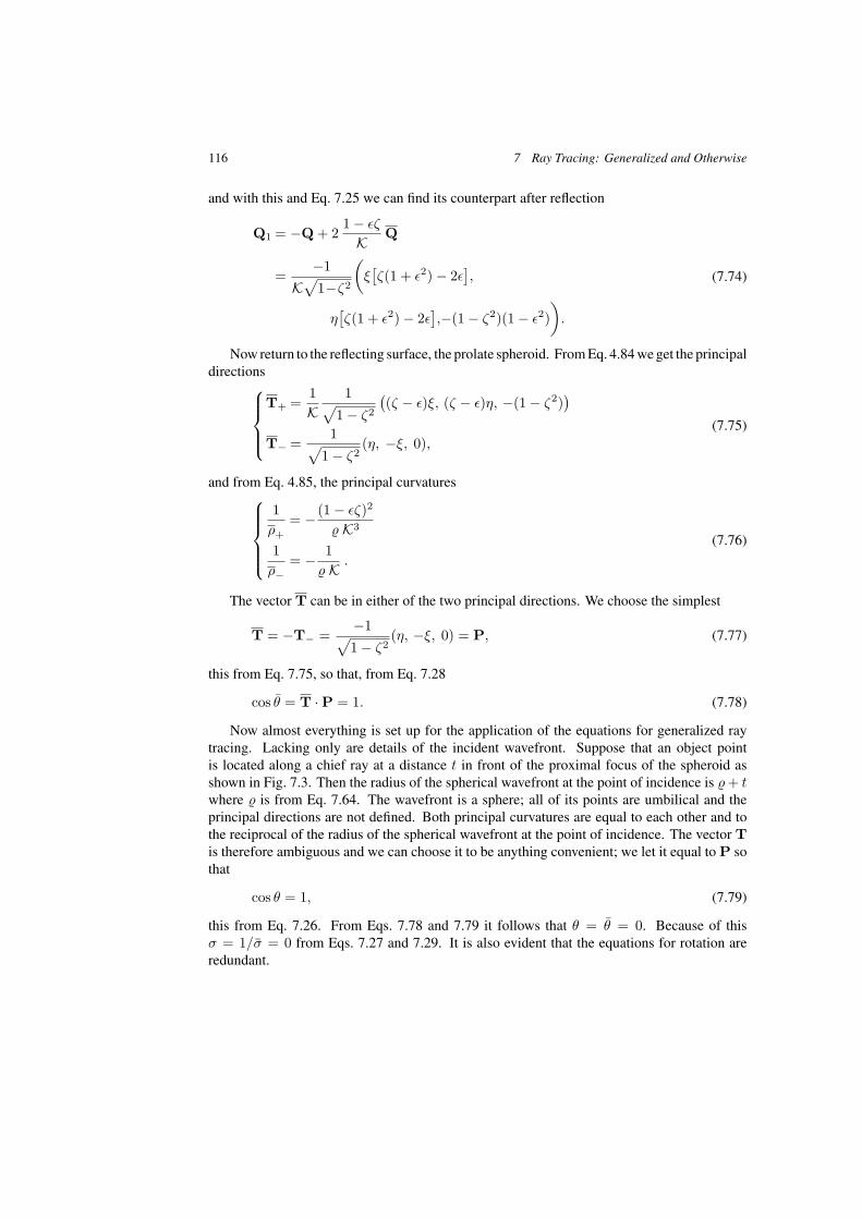
116 7 Ray Tracing: Generalized and Otherwise
and with this and Eq. 7.25 we can find its counterpart after reflection
Q1 = −Q + 21 − εζ
K Q
=−1
K√
1−ζ2
(ξ[ζ(1 + ε2) − 2ε
],
η[ζ(1 + ε2) − 2ε
],−(1 − ζ2)(1 − ε2)
).
(7.74)
Now return to the reflecting surface, the prolate spheroid. From Eq. 4.84 we get the principaldirections
T+ =
1K
1√1 − ζ2
((ζ − ε)ξ, (ζ − ε)η, −(1 − ζ2)
)T− =
1√1 − ζ2
(η, −ξ, 0),(7.75)
and from Eq. 4.85, the principal curvatures
1ρ+
= − (1 − εζ)2
� K3
1ρ−
= − 1� K .
(7.76)
The vector T can be in either of the two principal directions. We choose the simplest
T = −T− =−1√1 − ζ2
(η, −ξ, 0) = P, (7.77)
this from Eq. 7.75, so that, from Eq. 7.28
cos θ = T · P = 1. (7.78)
Now almost everything is set up for the application of the equations for generalized raytracing. Lacking only are details of the incident wavefront. Suppose that an object pointis located along a chief ray at a distance t in front of the proximal focus of the spheroid asshown in Fig. 7.3. Then the radius of the spherical wavefront at the point of incidence is � + twhere � is from Eq. 7.64. The wavefront is a sphere; all of its points are umbilical and theprincipal directions are not defined. Both principal curvatures are equal to each other and tothe reciprocal of the radius of the spherical wavefront at the point of incidence. The vector Tis therefore ambiguous and we can choose it to be anything convenient; we let it equal to P sothat
cos θ = 1, (7.79)
this from Eq. 7.26. From Eqs. 7.78 and 7.79 it follows that θ = θ = 0. Because of thisσ = 1/σ = 0 from Eqs. 7.27 and 7.29. It is also evident that the equations for rotation areredundant.
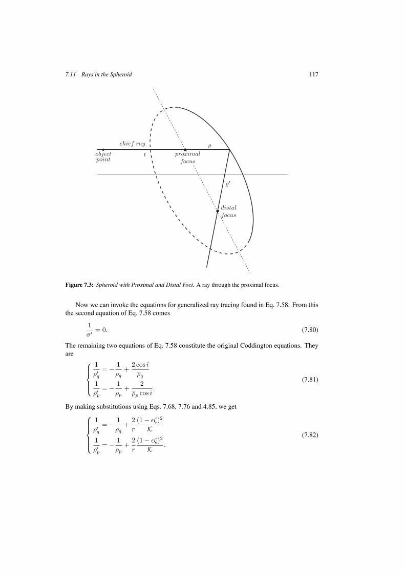
7.11 Rays in the Spheroid 117
Figure 7.3: Spheroid with Proximal and Distal Foci. A ray through the proximal focus.
Now we can invoke the equations for generalized ray tracing found in Eq. 7.58. From thisthe second equation of Eq. 7.58 comes
1σ′ = 0. (7.80)
The remaining two equations of Eq. 7.58 constitute the original Coddington equations. Theyare
1ρ′
q
= − 1ρq
+2 cos i
ρq
1ρ′
p
= − 1ρp
+2
ρp cos i.
(7.81)
By making substitutions using Eqs. 7.68, 7.76 and 4.85, we get
1ρ′
q
= − 1ρq
+2r
(1 − εζ)2
K1ρ′
p
= − 1ρp
+2r
(1 − εζ)2
K .
(7.82)

118 7 Ray Tracing: Generalized and Otherwise
In Eq. 7.76 we have identified ρ+ with ρp and ρ− with ρq.Now if the incident wavefront is a sphere then ρp = ρq = ρ, the sphere’s radius. In that
case ρ′p = ρ′
q and the reflected wavefront in the neighborhood of the traced ray has the propertythat the two principal curvatures are equal. That is not to say that the reflected wavefront isa sphere; only that it has an umbilical point at the traced ray. The radius of curvature of thewavefront at this point, say ρ′ is then given by this simpler version of Eq. 7.82
1ρ′ = −1
ρ+
2r
(1 − εζ)2
K . (7.83)
Suppose the object point is at the proximal focus so that ρ = �, where � is given in Eq. 7.64.Then from the above we get
1ρ′ =
1 − ε ζ
rK [−K + 2(1 − ε ζ)] =(1 − ε ζ)(1 − ε2)
rK =1�′ , (7.84)
where �′ is also found in Eq. 7.64. The image point is then at the distal focus, just as it shouldbe.
Now refer to Fig. 7.4 which shows the same ellipse encountered in the earlier illustrations.Assume that AB and BC are rays incident and reflected with point of incidence B. Supposethat the object point is at A and that its conjugate is at C. Let A be located a distance d in frontof the proximal focus and let C be at distance d′ in front of the distal focus. In what followswe adopt the usual optical convention that the curvature of a surface is positive if it is concaveto the right. Thus a converging wavefront has a positive curvature; if it diverges, its curvatureis negative. A wavefront originating at a point A will be spherical and its radius of curvatureat the point of incidence, B will be � + d; its curvature is negative. We know that the reflectedwavefront will have an umbilical point at B and that at that point its radius of curvature will be�′ −d′. Since it is converging the sign of its curvature will be positive. Then Eq. 7.83 becomes
1�′ + d′ = − 1
� + d+
2r
(1 − εζ)2
K . (7.85)
By taking the difference of Eqs. 7.83 and 7.85 we get the very useful formula
1�′ + d′ − 1
�′ = −(
1ρ − d
− 1ρ
), (7.86)
which reduces to, using Eqs. 7.64 and 7.66
d′ =drK2
(1 − ε2)[r(1 − ε2) − 2d(1 − εζ)2]. (7.87)
But what we really want is the reciprocal, the curvature of the wavefront and that is
1d′ = − (1 − ε2)
K2
[1 − ε2
t+ 2
(1 − εζ)2
r
]. (7.88)
These expressions will be seen again in Chapter 11 when they will be applied to the ModernSchiefspiegler.
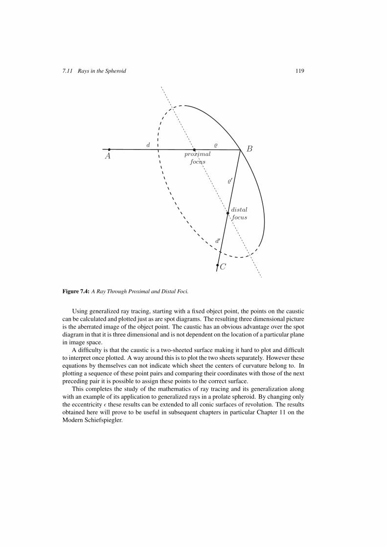
7.11 Rays in the Spheroid 119
Figure 7.4: A Ray Through Proximal and Distal Foci.
Using generalized ray tracing, starting with a fixed object point, the points on the causticcan be calculated and plotted just as are spot diagrams. The resulting three dimensional pictureis the aberrated image of the object point. The caustic has an obvious advantage over the spotdiagram in that it is three dimensional and is not dependent on the location of a particular planein image space.
A difficulty is that the caustic is a two-sheeted surface making it hard to plot and difficultto interpret once plotted. A way around this is to plot the two sheets separately. However theseequations by themselves can not indicate which sheet the centers of curvature belong to. Inplotting a sequence of these point pairs and comparing their coordinates with those of the nextpreceding pair it is possible to assign these points to the correct surface.
This completes the study of the mathematics of ray tracing and its generalization alongwith an example of its application to generalized rays in a prolate spheroid. By changing onlythe eccentricity ε these results can be extended to all conic surfaces of revolution. The resultsobtained here will prove to be useful in subsequent chapters in particular Chapter 11 on theModern Schiefspiegler.
The Mathematics of Geometrical and Physical Optics: The k-function and its Ramifications. O.N. StavroudisCopyright c© 2006 WILEY-VCH Verlag GmbH & Co. KGaA, WeinheimISBN: 3-527-40448-1
8 Aberrations in Finite Terms
Recall that the eikonal function is a measure of the optical path length between some arbitrarybut fixed object point and a point P in image space. In the notation we use, the coordinatesof the object point are never specified; the arguments of the function are the components of Pin image space. We have already seen that if P is a perfect image of the object point; everyray that passes through the object point must also passes through P. In that case the eikonalfunction is constant.
Solutions of the eikonal equation have been obtained previously in the form of a powerseries. Since perfect imagery requires the eikonal to be constant, all coefficients of the powerseries, except for the constant term, must be zero. It follows that non zero coefficients of thispower series must be measures of departures from perfect image formation. These coefficientshave come to be identified as aberrations; in the past they have proved to be eminently useful.Indeed, the third order Seidel aberrations or primary aberrations have been indispensable inoptical design for the better part of a century. In modern optical design these aberrationcoefficients have been extended to higher degrees.
But this power series has never been shown to converge nor even to be summable. It mayeven be that the series solution is asymptotic; that the series diverges but that a finite numberof terms provide a optimum approximation to real rays as determined by ray tracing. As far asI know this has never been successfully investigated.
In practice the aberration coefficients are calculated surface by surface in a lens designwith arguments that are not the coordinates of P but are heights and slopes of the marginaland principal paraxial rays that are traced through the system. So the result of all this is layersof approximations superimposed on earlier approximations. The miracle is that it not onlyworks but works exceedingly well. But as methods for designing lenses improve and as lensesbecome better and better the assumptions on which these techniques are based become lessvalid. The purpose of this chapter is to introduce a novel alternative.
We have already seen that the shape of the caustic surface depends on the k-functionand its first and second partial derivatives. We also know that the caustic can represent themonochromatic aberrations that we call image errors; spherical aberration, astigmatism andcoma. It follows then that all of these image errors are contained in the k-function. The fielderrors, distortion and field curvature, are determined by the location of the caustic in imagespace and this also is determined by the k-function. We conclude that all of the monochromaticaberrations reside in and can be determined by the k-function.
In all our discussions we have excluded color entirely as has been explained in the intro-ductory chapter. But we do not exclude the possibility that the k-function can be generalized to
122 8 Aberrations in Finite Terms
accommodate a dependence on wavelength and, in that case, provide a model for the chromaticaberrations.
So, we visualize the k-function as a closed form function of the variables v and w that is arepresentation of the total aberrations associated with an optical system relative to some fixedobject point. The coefficients of the commonly used infinite series expansion are identifiedwith various aberrations that had been observed in severely aberrated systems. Hence the titleof this chapter, Aberrations in Finite Terms.
8.1 Herzberger’s Diapoints
In Chapter 7 we mentioned spot diagrams, obtained by intersecting traced rays with a planein image space, and how it can be used to interpret the aberrations of an optical system.Herzberger proposed an alternative approach applicable only to rotationally symmetric opticalsystems. The plane determined by an off axis object point and the axis of rotational symmetryis called the meridional plane. Meridional rays are defined as those rays that lie entirely inthe meridional plane at every medium in an optical system. This can be seen from the raytracing equations for transfer (Eqs. 7.2 and 7.3) and for refraction (7.9 and 7.10). Skew raysare defined as those rays that are not meridional; rays that leave the object point at an angleto the meridional plane and pass through the optical system to image space where once againthey intersects the meridional plane. (They may also cross the meridional plane in the interiorof the lens.) The point of intersection of a skew ray with the meridional plane in image spaceis Herzberger’s diapoint.1
The totality of rays from a fixed object point that pass through the lens produce a distributionof diapoints on the meridional plane in image space just as they form a distribution of points ina spot diagram. Unlike the spot diagram, their distribution does not depend on the position ofan image plane; indeed, diapoints are useful in determining the best location of an image plane.On the other hand the spot diagram does provide a good approximation to the real image of apoint object.
8.2 Herzberger’s Fundamental Optical Invariant
This is a differential invariant that is valid for all optical systems, including off-axis telescopesand inhomogeneous media.2 Consider a lens that consists of three surfaces as shown in Fig. 8.1.The vectors Q, Q1, Q2, Q3, and Q′, all referred to some arbitrary coordinate origin, representpoints on a ray traced through the system. Moreover Q1, Q2, Q3, lie on the three refractingsurfaces; Q and Q′ are points in object space and image space, respectively that may or maynot be conjugates. Let n, n1, n2, and n′ be the refractive indices of the four media and letC, C1, C2 and C′ be the appropriate ray direction cosine vectors and let N1, N2, N3 be theunit normal vectors to the refracting surfaces at Q1, Q2, Q3, respectively. Now let λ, λ1, λ2and λ′ be the lengths of the ray segments between the points of incidence. Then, from the
1Herzberger 1946, Herzberger 1954.2Herzberger 1935, Stavroudis 1972a, Stavroudis 1972b.

8.2 Herzberger’s Fundamental Optical Invariant 123
Figure 8.1: Ray Through a Sample System. Shown is a ray – Q, Q1, Q2, Q3, Q′ – traced throughthis simple optical system. Refractive indices are n, n1, n2, and n′ where these media are separated bythe three surfaces. The lengths of the ray segments are λ, λ1, λ2 and λ′ so that its optical path length isnλ + n1λ1 + n2λ2 + n′λ′.
transfer equation from Chapter 7,
(7.2) P = P+λS,
as well as the refraction equation,
(7.9) S1 = S+γN,
the following ray tracing equations hold,
Q1 = Q + λC
Q2 = Q1 + λ1C1, n1C1 = n C + γ1N1
Q3 = Q2 + λ2C2, n2C2 = n1C1 + γ2N2
Q′ = Q3 + λ′C′, n′C′ = n2C2 + γ3N3.
(8.1)
Now assume that this ray is a member of a two-parameter family of rays that depends on theparameters p and q and then take the derivatives of the Q′s with respect to p. The result is,
∂Q1
∂p=
∂Q∂p
+ λ∂C∂p
+∂λ
∂pC
∂Q2
∂p=
∂Q1
∂p+ λ1
∂C1
∂p+
∂λ1
∂pC1
∂Q3
∂p=
∂Q2
∂p+ λ2
∂C2
∂p+
∂λ2
∂pC2
∂Q′
∂p=
∂Q3
∂p+ λ3
∂C3
∂p+
∂λ3
∂pC3
(8.2)
124 8 Aberrations in Finite Terms
Now scalar multiply the first of these by nC, the second by n1C1, the third by n2C2, and thefourth by n3C3 and add. Recall that C2
i = 1 so that ∂Ci/∂p · Ci = 0 so we get,
nC · ∂Q1
∂p+ n1C1 · ∂Q2
∂p, +n2C2 · ∂Q3
∂p+ n3C3 · ∂Q′
∂p
= nC · ∂Q∂p
+ n1C1 · ∂Q1
∂p+ n2C2 · ∂Q2
∂p+ n3C3 · ∂Q3
∂p
+n∂λ
∂p+ n1
∂λ1
∂p+ n2
∂λ2
∂p+ n3
∂λ3
∂p.
(8.3)
These are rearranged to get,
nC · ∂Q∂p
+∂Q1
∂p· (n1C1 − nC) +
∂Q2
∂p· (n2C2 − n1C1)
+∂Q3
∂p· (n3C3 − n2C2) − n3 C3 · ∂Q′
∂p+
∂L∂p
= 0.
(8.4)
where L is the optical path length, L = nλ + n1λ1 + n2λ2 + n3λ3.But from Eq. 8.1 niCi − ni−1Ci−1 = γiNi so that each term in Eq. 8.4 containing these
quantities is multiplied by ∂Qi/∂p. This is the derivative of a point on the refracting surfacewith respect to the arbitrary parameter and therefore is a vector tangent to the surface. Thescalar product of this with the normal vector Ni is zero so all of the terms in Eq. 8.4 vanishexcept for three, resulting in,
nC · ∂Q∂p
− n3C3 · ∂Q′
∂p+
∂L∂p
= 0. (8.5)
With respect to the second parameter q the exact same steps yield a second equation,
nC · ∂Q∂q
− n3C3 · ∂Q′
∂q+
∂L∂q
= 0. (8.6)
We assume that second derivatives exist and are continuous so that if we take the derivativeof Eq. 8.5 with respect to p and the derivative of Eq. 8.6 with respect to q and then eliminate∂2L/∂u∂v between them we get,
n′(
∂Q′
∂p· ∂C′
∂q− ∂Q′
∂q· ∂C′
∂p
)= n
(∂Q∂p
· ∂C∂q
− ∂Q∂q
· ∂C∂p
). (8.7)
The quantity,
n
(∂Q∂p
· ∂C∂q
− ∂Q∂q
· ∂C∂v
)(8.8)
has not only the same value in object and image space but also in every intermediate space inthe optical system. This is the Fundamental Optical Invariant.
8.3 The Lens Equation 125
8.3 The Lens Equation
Now lets let the points Q and Q′ lie on planes in object and image space that pass through thecoordinate origin so that z = z′ = 0. Set nC = S = (u, v, w), n′C′ = S′ = (u′, v′, w′)making S and S′ reduced direction cosine vectors. We have that Q = (x, y, , 0) and Q′ =(x′, y′, , 0) so that Eq. 8.7 becomes,
x′pu
′q + y′
pv′q − x′
qu′p − y′
qv′p = xpuq + ypvq − xqup − yqvp. (8.9)
This Herzberger called the direct method.3
The parameters p and q are arbitrary; they may take on any values we choose. We select forthese parameters all possible combinations of the object space variables, x, y, u, v resultingin a system of six equations,
x′xu′
y + y′xv′
y − x′yu′
x − y′yv′
x = 0
x′xu′
u + y′xv′
u − x′uu′
x − y′uv′
x = 1
x′xu′
v + y′xv′
v − x′vu′
x − y′vv′
x = 0
x′yu′
u + y′yv′
u − x′uu′
y − y′uv′
y = 0
x′yu′
v + y′yv′
v − x′vu′
y − y′vv′
y = 1
x′uu′
v + y′uv′
v − x′vu′
u − y′vv′
u = 0.
(8.10)
This can be expressed in Matrix form. Let M be given by,
M =
x′x x′
y x′u x′
v
y′x y′
y y′u y′
v
u′x u′
y u′u u′
v
v′x v′
y v′u v′
v,
(8.11)
and let J be the constant matrix,
J =
0 0 1 0
0 0 0 1
−1 0 0 0
0 −1 0 0
. (8.12)
Then Eq. 8.10 can be written as,
MJMT = J, (8.13)
where MT is the transpose of M. This I have called the lens equation.4 It is clear that |M| isthe Jacobian of this transformation.
3Herzberger 1943a, Herzberger 1943b.4Stavroudis 1972a, pp. 245–249.
126 8 Aberrations in Finite Terms
We can think of a lens as a device for mapping rays in object space into rays in image space.Recall that a ray is determined by a point on a reference plane, (x, y, , 0), and a direction,(u, v, w). We can think of this transformation as the system of equations,
x′ = x′(x, y, u, v)
y′ = y′(x, y, u, v)
u′ = u′(x, y, u, v)
v′ = v′(x, y, u, v).
(8.14)
Since conjoining two lenses results in yet another lens this system of transforms can be re-garded as a Lie group5, in which the identity element is simply the lack of a lens and theinverse transform is obtained by solving the equations in Eq. 8.14 for (x, y, u, v) in terms of(x′, y′, u′, v′).
We can go even further. Equation 8.13 is the defining equation for one of the two classicalmatrix groups, the symplectic group (the other being the orthogonal group).6 From Eq. 8.13we can show that M is a unitary matrix. Note first of all that |J | = 1 so that by taking thedeterminant of both members of Eq. 8.13 we get |M |2 = 1. It follows that M is non singular;inverses always exist.
We remarked earlier that a new lens was obtained where two lenses were conjoined. This isaccomplished by multiplying the corresponding two matrices. This works because the productof two Jacobian matrices is yet another Jacobian.
Suppose we decompose a lens into its elementary components, a sequence of alternatingoperations, refraction and transfer, each capable of being represented by a M matrix so thatthe lens could be represented by a matrix product. The idea was to apply this to the design ananalysis of lenses; like all such approaches to optical design it was far to complicated to beuseful.7
8.4 Aberrations in Finite Terms
This work is an extension and a continuation of work first published over twenty years ago.8
It is based on the general solution of the eikonal equation and the k-function, the expressionfor the wavefront train defined by that solution
(5.72) W(v, w; s) =q
n2 S − K,
where
(5.71) q = (ns−k)−(vkv + wkw) = (ns−k)+S·K.
5Stavroudis 1972a, pp. 285–286.6Stavroudis 1972a, pp. 286–288.7Stavroudis 1959.8Stavroudis and Fronczek 1978a.

8.5 Half-Symmetric, Symmetric and Sharp Images 127
and the caustic surface associated with that train,
(6.21) C±(v, w) =1
2n2 (H±S)S−K,
where,
(6.6) H = (n2−v2)kvv+(n2−w2)kww−2vwkvw,
where T 2 is the Hessian determinant,
(6.7) T 2 = kvvkww−k2vw,
and where S is the discriminant of a quadratic polynomial,
(6.15) S2 = H2−4n2u2T 2.
The parameter s in Eq. 5.71 is a distance measured from some fixed but arbitrary starting point.We choose this starting point to be one particular wave front in the train, which I’ve called
the archetype; with its optical path length from the ultimate object point equal to zero. This isof little importance in this chapter but will be useful in Chapter 9 which involves the refractionof the k-function. We are concerned with the structure of the caustic surface in which residesall of the properties, the aberrations if you will, of the wavefront train. These are uniquely andcompletely determined by the k-function.
The sign ambiguity, as we have already seen, shows that the caustic is a two sheeted surface.Equation 5.71 shows that there is a plane of symmetry. In what follows we will assume thatwe are dealing with an optical system possessing rotational symmetry and that the plane ofsymmetry is the meridional plane determined by some object point.
Herzberger used the distribution of diapoint to define a hierarchical system of aberrations.9
In general, the diapoints cover a region of the meridional plane. This he called deformationerror. If the diapoints collapse to an arc they form the half-symmetric image. If the arcdegenerates to a straight line the image is symmetric. Finally, if the straight line degeneratesto a single point the image is sharp.
8.5 Half-Symmetric, Symmetric and Sharp Images
Now recall the vector K = (0, kv, kw) a vector function of v and w that lies on the meridianalplane. Every ray in the system defined by Eq. 5.72 is associated with a particular pair of values,v and w, that define a value of the vector K that, in turn, defines a point on the meridionalplane. Therefore K defines the aggregate of diapoints associated with the system.
With no restrictions on K(v, w) it represents deformation error. We will impose restrictionson C±, given in Eq. 6.21, and observe their effect on K.
We first set T 2, defined in Eq. 6.7, equal to zero; T 2 is the Hessian determinant of thek-function. It can also be regarded as a Jacobian determinant of the two functions kv and kw
and its vanishing implies that a functional relation exists between them, say,
kw = f(kv). (8.15)
9Herzberger 1950.
128 8 Aberrations in Finite Terms
Then,
kvw = f ′ kvv
kww = f ′2 kvv,(8.16)
so that, from Eq. 6.6,
H = kvv[(n2 − v2) − 2vwf ′ + (n2 − w2)f ′2], (8.17)
and, from Eq. 6.21,{C+ = −K + 1
n2 H S
C− = −K.(8.18)
In this case the negative branch of the caustic surface, C−, degenerates into an arc on themeridional plane and is therefore the half-symmetric image.
Now consider Eq. 8.16 as a non linear first order partial differential equation. With themethod of Lagrange and Charpit that we derived in Chapter 5, we can get a complete integraland a general solution. First from Eq. 8.16 we define,
F = f(kv) − kw = f(p) − q = 0, (8.19)
that leads us to,
Fv = Fw = Fk = 0, Fp = f ′, Fq = −1.
As before we introduce the symbols p and q to represent the two partial derivatives. When thisis plugged into the characteristic equations Eq. 5.29 we get
dp
0=
dq
0=
−dv
f ′ =−dw
−1=
−dk
pf ′ − q.
The simplest of these and the one we choose to work with is dp = 0 which leads us to thecharacteristic p = α. This leads us to q = f(α), from Eq. 8.19, which we use in the totaldifferential equation,
dk = αdv + f(α)dw, (8.20)
which after integration yields the complete integral,
k(v, w) = αv + f(α)w + β(α), (8.21)
where α = α(v, w). By appending to this the side condition,
v + f ′(α) w + β′(α) = 0, (8.22)
we get the general solution. It follows that kv = α and kw = f(α), just as it should be.
8.5 Half-Symmetric, Symmetric and Sharp Images 129
From this we can see that K =(0, α, f(α)
)is the degenerate caustic and at the same time
the half-symmetric image. We take α to be the its parameter each value of which determinesone point on the half-symmetric image; at the same time each value of α determines a one-parameter family of rays that pass through that point.
The unit tangent vector to the half symmetric is obtained by differentiating K with respectto α. This we normalize to get the unit tangent vector
T(α) =
(0, 1, f ′(α)
)√
1 + f ′2 . (8.23)
When α is held fixed K is a point on the arc and T is its unit tangent vector at that point.Consider the totality of rays through that point; that is to say, for all those values of v and w forwhich α(v, w) = constant. The reduced direction cosine vector of these rays is, of courseS. The cosine of the angle, φ between one of these rays and the unit tangent vector T of thedegenerate caustic is given by,
cos φ =1n
(S · T) =v + f ′(α) w
n√
1 + f ′2 = − β′
n√
1 + f ′2 , (8.24)
from Eq. 8.23. But β′ and f ′ are both functions of α which is fixed. Therefore, cos φ isconstant for all rays that pass through a single point on the half-symmetric image; they mustthen make the same angle with its tangent and form a cone whose vertex is at that point. Thisis Herzberger’s theorem.10
If f and β are linear in α then the arc in Eq. 8.22 becomes a straight line and the image issymmetric. If α is constant the image is sharp; the rays defined by α(v, w) = constant allmust pass through the sharp image.
Now lets take a closer look at the sharp image. Refer now to Eq. 8.22 and note that,k = vkv + wκw + β. When we substitute this into Eq. 5.72, we get q = ns − β and
W(v, w) =1n2 (ns − β)S − (
0, α, F (α)), (8.25)
a train of concentric spherical wavefronts centered on the sharp image, exactly as it should.The sharp image occurs when s = β/n. This established a connection between Herzberger’ssystem of hierarchial aberrations and the k-function.
10Herzberger 1943b.
The Mathematics of Geometrical and Physical Optics: The k-function and its Ramifications. O.N. StavroudisCopyright c© 2006 WILEY-VCH Verlag GmbH & Co. KGaA, WeinheimISBN: 3-527-40448-1
9 Refracting the k-Function
In Chapter 5 we derived a general solution of the eikonal equation, in vector form that repre-sents a wavefront train in a homogeneous, isotropic medium. This general solution is almostuniversal; almost in that it cannot represent a train of plane wavefronts. In that case we mustuses the intermediate solution, the complete integral as did Luneburg.1 An immediate conse-quence of this solution is the vector equation for the caustic surface associated with this trainof wavefronts.
These expressions for wavefront and caustic depend in a natural way on two independentparameters, v and w, two of the three reduced ray direction cosines of the orthotomic systemof rays associated with the wavefront train; the third is u =
√n2 − v2 − w2. Another param-
eter is s, the geometric distance of a wavefront from some arbitrary but fixed starting point.Throughout all of this work this starting point is assumed to be the archetypical wavefront,defined as that unique wave front in the train whose optical path length from the ultimate objectpoint is zero. More will be said on this subject subsequently.
The immediate problem is to determine the effect a spherical refracting surface has on thek-function. In this chapter we will find the k-function, both for a plane wavefront train thatis refracted by a spherical refracting surface and a train of spherical wavefronts refracted bya refracting plane. Then we will deal with more general problem, the refraction of a train ofspherical wavefronts, originating at a finite object point, by a sphere.
An important thing to keep in mind is that the caustic surface, its shape and its location,tells us everything about the geometric aberrations associated with an optical system relative tosome fixed object point. Indeed, in Chapter 8 we have shown that components of the expressionfor the caustic can be identified with Herzberger’s diapoints.2
We now return to the general solution of the eikonal equation and the expression for thewavefront train in a homogeneous, isotropic medium
(5.72) W(v, w, s) =q
n2 S − K,
where
(5.71) q = ns−k+(
v∂k
∂v+ w
∂k
∂w
)= ns−k+S·K.
1Stavroudis 1972a, Chapter VIII.2Herzberger 1958, Chapters VII and XXVII.
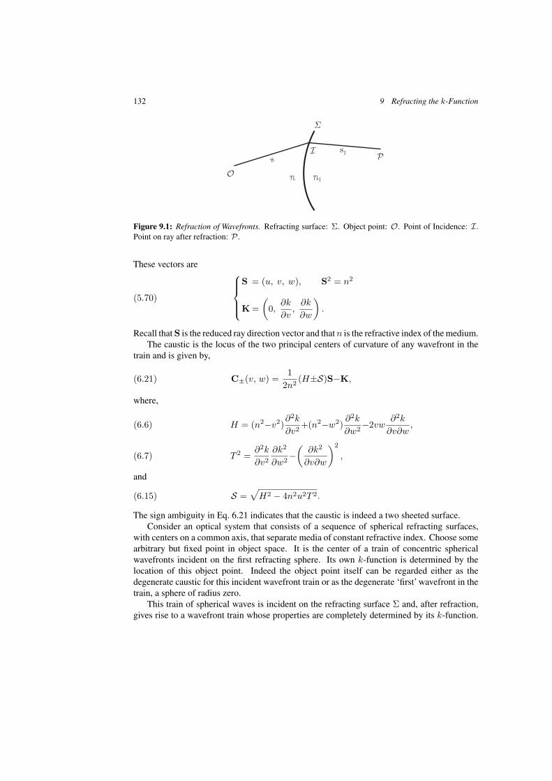
132 9 Refracting the k-Function
Figure 9.1: Refraction of Wavefronts. Refracting surface: Σ. Object point: O. Point of Incidence: I.Point on ray after refraction: P .
These vectors are
(5.70)
S = (u, v, w), S2 = n2
K =(
0,∂k
∂v,
∂k
∂w
).
Recall that S is the reduced ray direction vector and that n is the refractive index of the medium.The caustic is the locus of the two principal centers of curvature of any wavefront in the
train and is given by,
(6.21) C±(v, w) =1
2n2 (H±S)S−K,
where,
(6.6) H = (n2−v2)∂2k
∂v2 +(n2−w2)∂2k
∂w2 −2vw∂2k
∂v∂w,
(6.7) T 2 =∂2k
∂v2
∂k2
∂w2 −(
∂k2
∂v∂w
)2
,
and
(6.15) S =√
H2 − 4n2u2T 2.
The sign ambiguity in Eq. 6.21 indicates that the caustic is indeed a two sheeted surface.Consider an optical system that consists of a sequence of spherical refracting surfaces,
with centers on a common axis, that separate media of constant refractive index. Choose somearbitrary but fixed point in object space. It is the center of a train of concentric sphericalwavefronts incident on the first refracting sphere. Its own k-function is determined by thelocation of this object point. Indeed the object point itself can be regarded either as thedegenerate caustic for this incident wavefront train or as the degenerate ‘first’ wavefront in thetrain, a sphere of radius zero.
This train of spherical waves is incident on the refracting surface Σ and, after refraction,gives rise to a wavefront train whose properties are completely determined by its k-function.
9.1 Refraction 133
Let the object point be O and let I be the point of incidence on Σ and let O I be a ray as shownin Fig. 9.1. Let the geometric distance between O and I be s. Then ns is the optical pathlength to I where n is the refractive index of the first medium. The ray is refracted at I as itenters the second medium where the refractive index is n1. Take any point P on this refractedray and let s1 be the geometric distance from I to P . Then the optical path length along thisrefracted ray must be n1 s1 where n1 is the refractive index of the second medium. It followsthat the total optical path length from object point O to P is n s + n1 s1.
Earlier we defined the archetype wavefront as that unique wavefront in image space whoseoptical path measured from the object point is zero.3 Its location is therefore the geometricdistance,
s1 = −sn/n1, (9.1)
from the refracting surface. Since s1 is negative the archetype is to the left of the refractingsphere and is therefore virtual.
This wavefront train is then incident on the second spherical refracting surface giving riseto yet another refracted train in the next succeeding medium. This process is repeated until theimage space is reached after the final refracting surface.
Now refer back to the expression for the general wavefront in Eq. 5.72 in which the param-eter s appears. In each medium of the optical system this parameter will be measured from thearchetype4 in that medium. All conjugate wavefronts have the same optical path length, n s,measured from the appropriate archetype which leads us to,
ns = n1s1 = n2s2 = . . . . (9.2)
9.1 Refraction
In what follows we will be concerned with refraction at a single spherical refracting surface.5 Tokeep things simple the incident wavefront and its parameters will lack subscripts; the refractedwavefront and its parameters will be signaled by the subscript (1). In what follows r is theradius of the refracting sphere; the coordinate origin is taken at its center. We will write therefracted wavefront train as W1(v1, w1, s1) in the manner of Eq. 5.72 and q1, S1 and K1defined as in Eqs. 5.70 and 5.71.
It is obvious that any point lying on a refracting surface is its own image; every ray incidentat such a point must, after refraction, also pass through that point. It is clear that the opticalpath difference between that point and its image must be zero.
A wave front will intersect a refracting sphere in an arc. Choose any point on that curve;there the ray is normal to the wave front and is refracted by the sphere. Through that samepoint, the refracted ray is normal to the refracted wave front.
The optical path distance from any point on the archetype, along a ray, to its point ofintersection with a wave front, is constant. Refer now to the point on this refracting surface,through which two wave fronts pass, one before refraction and one after. The optical path
3Stavroudis and Fronczek 1976.4Stavroudis 1995a.5Stavroudis 1995b.
134 9 Refracting the k-Function
difference between this point before refraction and its image after refraction was shown to bezero. It follows that the optical path distance from any point on the incident wavefront, alongan incident ray and its refracted counterpart, to the refracted wave front, must also equal zero.We have shown that any two wave fronts that pass through a point on a refracting surface mustbe conjugates and therefore, from Eq. 9.1, s1 = −sn/n1. This result we will use later
Now refer back to Chapter 7, on ray tracing. Recall
(7.9) S1 = S+γN,
and
(7.10) γ = S1·N−S·N = n1 cos r−n cos i,
where i is the angle of incidence and where r is the angle of refraction. The two vectors, Sand S1 are referred to as reduced direction vectors. By writing Eq. 7.9 as γN = S1 − S andsquaring both sides we get
γ2 = (S1 − S)2 = n21 + n2 − 2α, (9.3)
where
α = S1 · S = uu1 + vv1 + ww1. (9.4)
9.2 The Refracting Surface
Our goal is to obtain k1(v1, w1) from k(v, w) when the latter is known.6 To do so we needtwo vector functions to represent the refracting sphere, one in terms of v and w associated withthe incident wavefront train, the other in terms of v1 and w1 the parameters for the refractedwavefronts. The first of these involves k(v, w) and its derivatives; the second, k1(v1, w1).Since both are representations of the same surface we are able to equate the two and obtain therequired relationships.
The equation of a sphere centered at the coordinate origin is,
F = P2 − r2 = 0. (9.5)
Its gradient is normal to the surface so that the unit normal vector N is then,
N =∇F√(∇F)2
=1rP. (9.6)
We next substitute the expression for the incident wavefront train, Eq. 5.74, into the equationfor the sphere, Eq. 9.5 and get a quadratic equation in q,
q2 − 2aq + n2(b2 − r2) = 0, (9.7)
6Stavroudis 1969.
9.2 The Refracting Surface 135
where
a = v∂k
∂v+ w
∂k
∂w
b2 =(
∂k
∂v
)2
+(
∂k
∂w
)2
.
(9.8)
The solution of Eq. 9.7 is,
q = a − ∆, (9.9)
where
∆2 = a2 − n2(b2 − r2). (9.10)
In Eq. 9.8 we defined a and b. By comparing Eqs. 9.9 and 5.71 we can see that
k − ns = ∆. (9.11)
We have chosen the negative branch of the quadratic solution to place the point of incidencenearer to the vertex of the refracting surface. By substituting the value of q from Eq. 9.9 intoEq. 5.72 we get the equation for the refracting surface in terms of the parameters of the incidentray,
P(v, w) =1n2 (a − ∆)S − K. (9.12)
We go through exactly the same steps for the refracted wavefront train to get,
q21 − 2a1q1 + n2
1(b21 − r2) = 0, (9.13)
an analog of Eq. 9.7, whose solution is (we again choose the negative branch), referring toEq. 5.71,
q1 = n1s1 − k1 + a1 = a1 − ∆1, (9.14)
where,
a1 = v1∂k1
∂v1+ w1
∂k1
∂w1
b21 =
(∂k1
∂v1
)2
+(
∂k1
∂w1
)2
∆21 = a2
1 − n21(b
21 − r2).
(9.15)
We also get the analog of Eq. 9.12
P1(v1, w1) =1n2
1(a1 − ∆1)S1 − K1 (9.16)
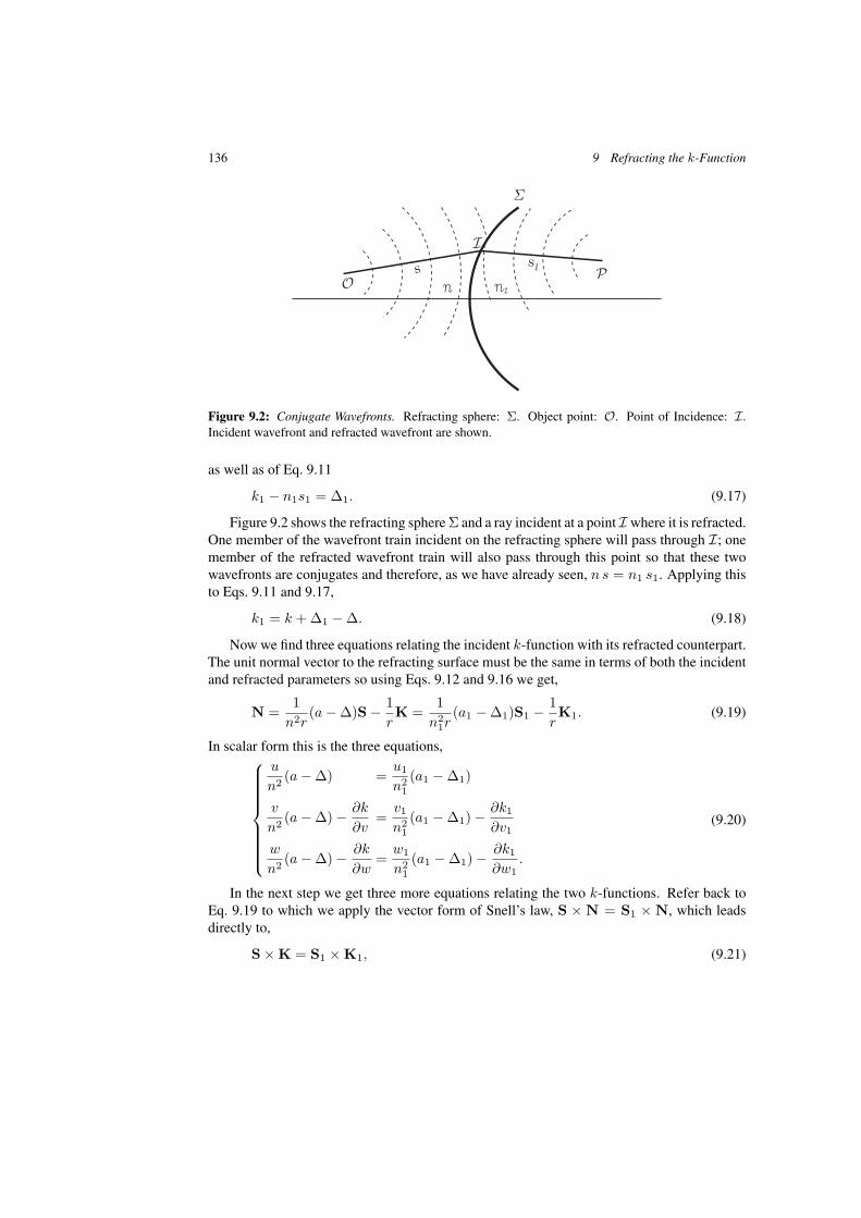
136 9 Refracting the k-Function
Figure 9.2: Conjugate Wavefronts. Refracting sphere: Σ. Object point: O. Point of Incidence: I.Incident wavefront and refracted wavefront are shown.
as well as of Eq. 9.11
k1 − n1s1 = ∆1. (9.17)
Figure 9.2 shows the refracting sphere Σ and a ray incident at a point I where it is refracted.One member of the wavefront train incident on the refracting sphere will pass through I; onemember of the refracted wavefront train will also pass through this point so that these twowavefronts are conjugates and therefore, as we have already seen, n s = n1 s1. Applying thisto Eqs. 9.11 and 9.17,
k1 = k + ∆1 − ∆. (9.18)
Now we find three equations relating the incident k-function with its refracted counterpart.The unit normal vector to the refracting surface must be the same in terms of both the incidentand refracted parameters so using Eqs. 9.12 and 9.16 we get,
N =1
n2r(a − ∆)S − 1
rK =
1n2
1r(a1 − ∆1)S1 − 1
rK1. (9.19)
In scalar form this is the three equations,
u
n2 (a − ∆) =u1
n21(a1 − ∆1)
v
n2 (a − ∆) − ∂k
∂v=
v1
n21(a1 − ∆1) − ∂k1
∂v1
w
n2 (a − ∆) − ∂k
∂w=
w1
n21(a1 − ∆1) − ∂k1
∂w1.
(9.20)
In the next step we get three more equations relating the two k-functions. Refer back toEq. 9.19 to which we apply the vector form of Snell’s law, S × N = S1 × N, which leadsdirectly to,
S × K = S1 × K1, (9.21)

9.3 The Partial Derivatives 137
which in scalar form is,
w1∂k1
∂v1− v1
∂k1
∂w1= w
∂k
∂v− v
∂k
∂w
u1∂k1
∂v1= u
∂k
∂v
u1∂k1
∂w1= u
∂k
∂w.
(9.22)
These seven equations, Eqs. 9.18, 9.20 and 9.22 are precisely the equations that relate thek-function of the incident wavefront train to that of the refracted wavefront train.
9.3 The Partial Derivatives
By eliminating ∂k/∂v and ∂k/∂w between the three equation of Eq. 9.22 we obtain
(u1w − uw1)∂k1
∂v1− (u1v − uv1)
∂k1
∂w1= 0, (9.23)
which tells us that there must be some factor A such that
∂k1
∂v1= A(u1v − uv1),
∂k1
∂w1= A(u1w − uw1). (9.24)
This in turn leads us to, using Eq. 9.22
∂k
∂v=
u1
uA(u1v − uv1),
∂k
∂w=
u1
uA(u1w − uw1). (9.25)
Now if we let
A = B/u1 (9.26)
these partial derivatives take a more symmetric form
∂k
∂v=
B
u(u1v − uv1),
∂k
∂w=
B
u(u1w − uw1) (9.27)
and
∂k1
∂v1=
B
u1(u1v − uv1),
∂k1
∂w1=
B
u1(u1w − uw1). (9.28)
From the first equation of Eq. 9.20 we get
a − ∆n2 =
u1
u
a1 − ∆1
n21
, (9.29)
138 9 Refracting the k-Function
which, when substituted into the second equation in Eq. 9.20 yields
vu1
u
a1 − ∆1
n21
− B
u(u1v − uv1) = v1
a1 − ∆1
n21
− B
u1(u1v − uv1)
a1 − ∆1
n21
(u1v − uv1) = B(u1v − uv1)u1 − u
u1
a1 − ∆1
n21
= Bu1 − u
u1,
(9.30)
where Eqs. 9.24 and 9.25 have been used. From this and Eq. 9.26 it also follows that
a − ∆n2 = B
u1 − u
u. (9.31)
The third equation of 9.20 yields identical results. Note that by eliminating B(u1 −u) betweenEqs. 9.30 and 9.31 we get back the first equation of Eq. 9.20.
Next we apply the results of Eq. 9.31 to Eqs. 9.8 and 9.10 to get
a =B
u(n2u1 − αu)
b2 =B2
u2 (n2u21 + n2
1u2 − 2αuu1)
∆2 = B2(α2 − n2n21) + r2n2
(9.32)
and from Eqs. 9.15 and 9.27 the result is
a1 =B
u1(αu1 − n2
1u)
b21 =
B2
u21
(n2u21 + n2
1u2 − 2αuu1)
∆21 = B2(α2 − n2n2
1) + r2n21,
(9.33)
where α is defined in Eq. 9.4.Now go back to Eq. 9.31 and rewrite it as
u∆ = ua − n2B(u1 − u), (9.34)
to which we apply the first equation of Eq. 9.32 to get
∆ = B(n2 − α). (9.35)
Now we square both sides and use the third equation of Eq. 9.32. The result is
∆2 = B2(α2 − n2n21) + r2n2 = B2(n2 − α)2. (9.36)

9.3 The Partial Derivatives 139
This we solve for B
B2 =r2n2
(n2 − α)2 − (α2 − n2n21)
, (9.37)
which reduces to
B2(n2 + n21 − 2α) = B2γ2 = r2, (9.38)
where we have used γ defined in Eq. 9.3. Our result is an expression for B
B = r/γ, (9.39)
where we have chosen the positive branch of the square root.We substitute this value of B into Eq. 9.27
∂k
∂v=
r
uγ(v1u − vu1)
∂k
∂w=
r
uγ(w1u − wu1),
(9.40)
and again into Eq. 9.28
∂k1
∂v1=
r
u1γ(v1u − vu1)
∂k1
∂w1=
r
u1γ(w1u − wu1),
(9.41)
as well as Eq. 9.32
a =r
uγ(αu − n2u1)
b2 =r2
u2γ2 (n21u
2 + n2u21 − 2αuu1)
∆ =−r
γ(n2 − α),
(9.42)
and Eq. 9.33
a1 =r
u1γ(n2
1u − αu1)
b21 =
r2
u21γ
2 (n21u
2 + n2u21 − 2αuu1)
∆1 =r
γ(n2
1 − α).
(9.43)

140 9 Refracting the k-Function
In both Eqs. 9.42 and 9.43 square roots were taken to obtain ∆ and ∆1. The signs were chosenin such a way as to be consistent with Eq. 9.18 which, after the appropriate substitutions,becomes
k1 = k + ∆1 − ∆
= k +r
γ[(n2
1 − α) + (n2 − α)]
= k +r
γ(n2
1 + n2 − 2α)
= k + rγ.
(9.44)
Again we use the equation for γ in Eq. 9.3.
9.4 The Finite Object Point
As we did in Chapter 6 we choose an object point with the coordinates(0,−h, −(t + r)
), the
starting point of the wavefront train, so that s = 0 as shown in Fig. 9.3. It can also be thoughtof as the caustic associated with this wavefront train. This point can also be thought of as adegenerate spherical wavefront of radius zero. Now write Eq. 5.69 in scalar form equating thecomponents equal to the coordinates of the object point. This results in,
x = (q/n2)u = 0
y = (q/n2)v − ∂k
∂v= −h
z = (q/n2)w − ∂k
∂w= −(t + r).
(9.45)
From the first of these it must be that, from Eq. 5.72, recalling that s = 0
q = −k +(
v∂k
∂v+ w
∂k
∂w
)= 0, (9.46)
and from the second and third equations we can see that,
∂k
∂v= h,
∂k
∂w= t + r. (9.47)
When this is applied to Eq. 9.46 we get,
k = vh + w(t + r). (9.48)
We next apply the relations in Eq. 9.47 to Eq. 9.40 and get,{r(v1u − vu1) = uγh
r(w1u − wu1) = uγ(t + r).(9.49)
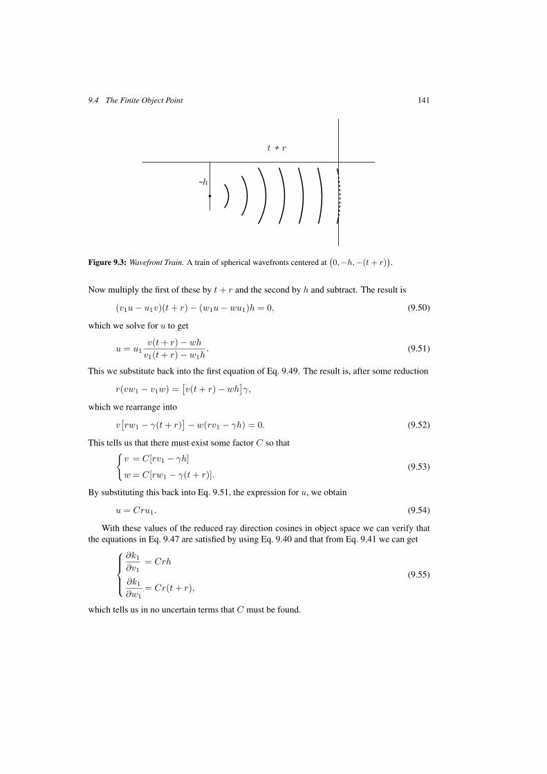
9.4 The Finite Object Point 141
Figure 9.3: Wavefront Train. A train of spherical wavefronts centered at(0, −h, −(t + r)
).
Now multiply the first of these by t + r and the second by h and subtract. The result is
(v1u − u1v)(t + r) − (w1u − wu1)h = 0, (9.50)
which we solve for u to get
u = u1v(t + r) − wh
v1(t + r) − w1h. (9.51)
This we substitute back into the first equation of Eq. 9.49. The result is, after some reduction
r(vw1 − v1w) =[v(t + r) − wh
]γ,
which we rearrange into
v[rw1 − γ(t + r)
] − w(rv1 − γh) = 0. (9.52)
This tells us that there must exist some factor C so that{v = C[rv1 − γh]
w = C[rw1 − γ(t + r)].(9.53)
By substituting this back into Eq. 9.51, the expression for u, we obtain
u = Cru1. (9.54)
With these values of the reduced ray direction cosines in object space we can verify thatthe equations in Eq. 9.47 are satisfied by using Eq. 9.40 and that from Eq. 9.41 we can get
∂k1
∂v1= Crh
∂k1
∂w1= Cr(t + r),
(9.55)
which tells us in no uncertain terms that C must be found.
142 9 Refracting the k-Function
9.5 The Quest for C
First we calculate u2 + v2 + w2 using Eqs. 9.53 and 9.54 to get
n2 = C2{r2n21 − 2rγ[hv1 + w1(t + r)] + γ2[h2 + (t + r)2]}
which we rearrange into a quadratic polynomial in γ
γ2C2[h2 + (t + r)2] − 2γrC2[hv1 + w1(t + r)] + C2r2n21 − n2 = 0. (9.56)
Next comes α from Eq. 9.4
α = C{rn2
1 − γ[v1h + w1(t + r)]}, (9.57)
which we plug into the expression for γ2 from Eq. 9.3 resulting in
γ2 = n21 + n2 − 2C
{rn2
1 − γ[v1h + w1(t + r)]}
which we rearrange into another quadratic polynomial in γ
γ2 − 2Cγ[v1h + w1(t + r)] − [n21 + n2 − 2Crn2
1] = 0. (9.58)
Between these two polynomials we eliminate γ yielding an equation involving C alone.To do this we use Sylvester’s dialectic method7 described also in the Appendix. But first
to simplify matters we make the following definitions:{M = v1h + w1(t + r)
N = h2 + (t + r)2,(9.59)
so that the two polynomials, Eqs. 9.56 and 9.58 become{γ2C2N − 2γrC2M + C2r2n2
1 − n2 = 0
γ2 − 2γCM − (n21 + n2 − 2Crn2
1) = 0.(9.60)
Sylvester’s eliminant between the two equations of Eq. 9.60 is the following determinantequation∣∣∣∣∣∣∣∣∣∣∣
C2N −2rC2M C2r2n21 − n2 0
1 −2CM −(n21 + n2 − 2Crn2
1) 0
0 C2N −2rC2M C2r2n21 − n2
0 1 −2CM −(n21 + n2 − 2Crn2
1)
∣∣∣∣∣∣∣∣∣∣∣=
∣∣∣∣∣C2N −2rC2M
1 −2CM
∣∣∣∣∣∣∣∣∣∣−2C2rM C2r2n2
1 − n2
−2CM −(n2 + n21 − 2Crn2
1)
∣∣∣∣∣−
∣∣∣∣∣C2N C2r2n2
1 − n2
1 −(n2 + n21 − 2Crn2
1)
∣∣∣∣∣2
= 0. (9.61)
7See, for example, Ito 1993, Vol. 1, pp. 369E.
9.5 The Quest for C 143
After a long sequence of calculations this reduces to the sextic polynomial equation
4n21Nr2a1C
6 − 4ra1a3C5 + (4M2a4 − a2
3)C4 (9.62)
− 4n2ra1C3 + 2n2a3C
2 − n4 = 0,
where
a1 = M2 − n21N
a2 = N + r2
a3 = n2N + n21a2
a4 = n21r
2 + n2a2.
(9.63)
For convenience let,
m1 = v1h + w1(t + r). (9.64)
When this and Eqs. 9.53, 9.54 and 9.8 are substituted into Eq. 9.48 we find that,
k =(
u
u1
) (m1 − γ
rb2
), (9.65)
which, when applied to Eq. 9.44, yields,
k1 =(
u
u1
)m1 +
γ
r
[r2 −
(u
u1
)b2
]. (9.66)
Next square each of the equations in Eqs. 9.53 and 9.54 and add to get,
n2 =(
u
u1
)2 [n2
1 − 2m1γ
r+
(γ
r
)2b2
], (9.67)
where we have used u2 + v2 + w2 = n2 and u21 + v2
1 + w21 = n2
1.Next substitute Eq. 9.54 into Eq. 9.55 we find that,
∂k1
∂v1=
(u
u1
)h ,
∂k1
∂w1=
(u
u1
)(t + r). (9.68)
By eliminating u/u1 from the two equations in Eq. 9.68 we get the rather remarkable result,
(t + r)∂k1
∂v1− h
∂k1
∂w1= 0, (9.69)
a linear, first order, partial differential equation with constant coefficients. By using the methodof Lagrange we find its general solution to be an arbitrary function of its characteristic m1,defined in Eq. 9.64. The derivatives of k1(m1) are then,
∂k1
∂v1= k′
1h,∂k1
∂w1= k′
1(t + r), (9.70)

144 9 Refracting the k-Function
where k′1 denotes the derivative of k1 with respect to m1. By comparing the derivatives in
Eq. 9.68 with those in Eq. 9.70 we see that,
k′1 = u/u1. (9.71)
When we apply these to Eq. 9.15 we get,
a1 = k′1m1, (9.72)
and,
b21 = k′2
1 b2. (9.73)
Next refer back to Eq. 9.58 into which we substitute from Eqs. 9.55, 9.64, 9.70 and 9.77,below, to get the quadratic polynomial equation,
rγ2 − 2m1k′1γ − rM = 0. (9.74)
A second quadratic polynomial equation results when the same substitution along with Eqs. 9.8and 9.47 is made into Eq. 9.56,
b2k′21 γ2 − 2rm1k
′21 γ + r2(n2
1k′21 − n2) = 0, (9.75)
Now refer back to Eqs. 9.43 and 9.57 in which we substitute from Eq. 9.73 to get,
b21 = k′2
1 b2 =r2
γ2 [k′1 + (n2
1k′1 − n2)(k′
1 − 1)],
or,
k′1(k
′1b
2γ2 − r2) = r2(n21k
′1 − n2)(k′
1 − 1). (9.76)
In exactly the same way Eq. 9.59 becomes,
M = n2 + n21 − 2 n2
1k′1, (9.77)
and Eq. 9.66 turns into,
r(k1 − k′1m1) = γ(r2 − k′
1b2). (9.78)
9.6 Developing the Solution
The first step is to eliminate γ from the various polynomial equations given above usingEqs. 9.76 and 9.78 which take the form,
γ = rm1 k′
1 − k1
b2 k′1 − r2 , γ2 = r2 (n2
1 k′1 − n2)(k′
1 − 1)k′1 (b2 k′
1 − r2). (9.79)
9.6 Developing the Solution 145
When we eliminate γ between the two equations in Eq. 9.79 we get,
(b2 k′1 − r2)(n2
1 k′1 − n2)(k′
1 − 1) = k′1(m1 k′
1 − k1)2. (9.80)
Next substitute the expressions in Eq. 9.79 into the polynomial equation in Eq. 9.76 to get,
r2(n21 k′
1 − n2)(k′1 − 1) − 2m1k
′21 (m1 k′
1 − k1) − k′1(b
2k′1 − r2)M = 0; (9.81)
the same substitution into Eq. 9.75 results in,
b2 k′1(n
21 k′
1 − n2)(k′1 − 1) − 2 m1k
′21 (m1k
′1 − k1) (9.82)
+ (b2k′1 − r2)(n2
1k′21 − n2) = 0.
Now let,
L = (n21 k′
1 − n2)(k′1 − 1). (9.83)
Then,
dL
dk′1
= n1(k′1 − 1) + n′
1 k′1 − n2 = −M. (9.84)
When these are substituted into Eq. 9.81 we get,
r2L − 2m1k′21 (m1k
′1 − k1) + k′
1(b2k′2
1 − r2)dL/dk′1 = 0,
which turns into,
d
d k′1
[L
k′1(b2k′
1 − r2)]
− 2m1(m1k′1 − k1) = 0. (9.85)
Now note that,
k′′1
d
d k′1
=d
dm1and
d
dm1(m1k
′1 − k1)2 = 2k′
1(m1k′1 − k1),
so that k′′1 is an integrating factor for Eq. 9.85,
d
dm1
[L
k′1(b2k′
1 − r2) − (m1k′1 − k1)2
]= 0.
A quadrature results in,
(b2k′1 − r2)(n2
1 k′1 − n2)(k′
1 − 1) = k′1(m1k
′1 − k1)2 + A2 k′
1 (9.86)
where A is a constant of integration. Here we have used Eq. 9.83.
146 9 Refracting the k-Function
9.7 Conclusions
In this chapter we have attempted to determine the k-function of a refracted wavefront train,k1(v1, w1) from that of an incident wavefront train, k(v, w). A number of abstract relationsbetween these two functions have been found but exact relations are not obtainable withoutspecific knowledge of the incident k-function. We had simplified the calculations by placingthe coordinate origin at the center of the refracting sphere.
The idea of the conjugate wavefronts was also introduced. Its definition is reflective,symmetric and transitive and so is an equivalence relation8 that partitions the wavefront trainin an optical system, that arises from some fixed object point, into disjoint equivalence classes,each of which containing exactly one member of the wavefront train in each of the media. Inthis context the archetypical wavefronts all belong to the same equivalence class.
The ultimate goal of this effort is to develop a system of optical design. The work presentedhere and in previous papers is, by no means complete. The obvious next step is to obtainsolutions for k1 for specific objects, namely, the finite object point and the object point atinfinity. These refracted wavefront trains will then be incident on the next refracting surfacepresenting yet another problem to be solved using the general methods described here.
That only spherical refracting surfaces were considerd may seem to be an unnecessaryrestriction, a restriction that excludes much of modern optics. Ultimately we plan to extendthese results to at least conic surfaces as well as to systems that are not rotationally symmetric.
8Ibid. pp. 530–531.
The Mathematics of Geometrical and Physical Optics: The k-function and its Ramifications. O.N. StavroudisCopyright c© 2006 WILEY-VCH Verlag GmbH & Co. KGaA, WeinheimISBN: 3-527-40448-1
10 Maxwell Equations and the k-Function
About a century ago Hertz solved the Maxwell equations for a train of spherical wavefrontsand in doing so he introduced the concept of the vector and scalar potential functions.1 He didthis by first converting the arguments of the Maxwell equations from Cartesian to sphericalcoordinates, obtained a wave equation for the potential functions and found a solution thatseparates in a natural way into a near field solution that anticipated the dipole oscillator, and afar field solution that forms the basis of modern antenna theory.
In Chapter 5 we developed a formula for a wavefront train in a homogeneous isotropicmedium as a general solution of the eikonal equation, expressed as a vector function of position.In Chapter 6 we investigated the geometry of these wavefronts and obtained the equation ofthe caustic surface.
To recapitulate: By holding s fixed and allowing v and w to vary we generate a surfacethat is one of the wavefronts in the train. The wavefront train is then a one-parameter familyof these surfaces with s as its parameter. On the other hand if we hold v and w fixed, theexpression becomes the equation of a point on the ray, normal to each of the wavefronts in thetrain, with s as its variable. From this point of view the totality of rays associated with thewavefront train is a two-parameter family of rays with v and w as the parameters. In Chapter 3we have referred to such a system as an orthotomic system or as a normal congruence.
The obvious question is whether Hertz’s method can be repeated for this more generalcase. The first step is to define a system of generalized coordinates based on the solution of theeikonal equation. To do this we assume that through every point (x, y, z) in space (or at leastthat part of space that interests us) there passes exactly one wavefront, thus fixing the value ofthe parameter s. This assumption may fail in the neighborhood of a caustic raising a problemthat will be discussed later. The location of the point on the wavefront is determined by twoother parameters, v and w. This enables us to treat s, v and w as generalized coordinates of apoint in space subject to certain reservations in the neighborhood of the caustic.
Now we are able to express gradient, divergence and curl in terms of these new coordinates.The obvious approach is to follow in Hertz’s footsteps, to derive the vector and scalar potentialfunctions, but this leads us to a second order wave equation which, unlike the one obtained byHertz, can best be described as intractable.
A direct approach is more suitable, leading to expressions for E, the electric field vector,and H, the magnetic field vector. These are manageable and depend on the k-function as wellas an additional arbitrary vector function V that is subject to several conditions, as we willshow.
1Joos 1941, pp. 322ff. Most modern references start with the dipole oscillator and deduce the spherical wavefronts,such as Marion and Heald 1980, pp. 232–245.

148 10 Maxwell Equations and the k-Function
10.1 The Wavefront
From the general solution of the eikonal equation we obtained the vector function for thewavefront train
(5.72) W(v, w, s) =q
n2 S−K,
where
(5.70)
{S = (u, v, w)
K = (0, kv, kw),
and where the scalar factor is,
(5.71) q = ns−k+(vkv+wkw) = ns−k+S·K.
For each s, this vector function of two parameters represents a surface in space and issubject to analysis by the general methods of differential geometry as described in Chapter 5.This surface is a member of the one-parameter train of wavefronts whose parameter is s.
The derivatives of W are the vectors Wv and Ww tangent to the wavefront and Ws as itsnormal so that Wv · Ws = Ww · Ws = 0; Ws being a unit normal vector of the wave frontand is therefore a ray direction cosine vector. Note also that,
(4.7) Ws =1D
(Wv×Ww) =1nS.
where,
(4.8) D2 = (Wv×Ww)2.
10.2 The Maxwell Equations
We begin with the well-known Maxwell equations for homogeneous, isotropic media,2
∇ × E = −µ
c
∂H∂t
∇ · E = 0
∇ × H =ε
c
∂E∂t
∇ · H = 0
(10.1)
where ε and µ are constant and are related to the refractive index by n =√
εµ.Since we will be dealing with derivatives with respect to s, the distance parameter, rather
than the time parameter t, a change of variables from t to s is needed. This is done with
∂
∂t=
ds
dt
∂
∂s= v
∂
∂s=
c
n
∂
∂s, (10.2)
2Stavroudis 1972, Chapters VIII and IX. A general solution using the method of Lagrange and Charpit; a detailedaccount can be found in Forsyth 1996, Chapter IX. See also Stavroudis 1995.
10.3 Generalized Coordinates and the Nabla Operator 149
where v is the velocity of light in this medium. The two Maxwell equations that involve thecurl operator are changed into
∇ × E = −µ
c
∂H∂t
= −√
µ
ε
∂H∂s
∇ × H =ε
c
∂E∂t
=√
ε
µ
∂E∂s
.
(10.3)
10.3 Generalized Coordinates and the Nabla Operator
We have already discussed the generalized coordinates, v, w and s, induced by the solution ofthe eikonal equation. The nabla operator can then be expressed in terms of these generalizedcoordinates and therefore so can the Maxwell equations.
We now return to the caveat mentioned earlier. In the first place the transformation fromcartesian coordinates to generalized coordinates is not always single valued; through each pointin space there may pass more than one wavefront belonging to the train. As we have alreadystated, this is certainly true in the neighborhood of a caustic, a cusp locus of the wavefronttrain.3 However we are concerned with not only the point in space but also with only one ofthe wavefronts that passes through it. This appears to remove the mathematical ambiguity.Diffractive interference between wavefronts passing through that point is certainly likely butat this point we can do no more than speculate on its nature.
From here on we will refer to the generalized coordinates v, w, and s. Now assume thatsome function f depends on these, so that,
fv = ∇f · Wv, fw = ∇f · Ww, fs = ∇f · Ws. (10.4)
Multiply the second of these by Wv the first, by Ww and subtract to get,
fwWv − fvWw = (∇f · Ww)Wv − (∇f · Wv)Ww
= ∇f × (Wv × Ww) = D(∇f × Ws).(10.5)
By taking the vector product of this expression with Ws and using the third equation in Eq. 10.4we get,
∇f =1D
[(Ww × Ws)fv − (Wv × Ws)fw
]+ Wsfs (10.6)
where D is defined in Eq. 4.8.It can also be shown that divergence and curl in terms of these generalized coordinates are
∇ · V =1D
[(Ww × Ws) · Vv − (Wv × Ws) · Vw
]+ Ws · Vs. (10.7)
and
∇ × V =1D
[(Ww × Ws) × Vv − (Wv × Ws) × Vw
]+ Ws × Vs. (10.8)
3Stavroudis et al. 1978.

150 10 Maxwell Equations and the k-Function
We also have the directional derivative
(P · ∇)A =1D
[(Ws × P) · Ww Av − (Ws × P) · Wv Aw
]+ (Ws · P) As.
(10.9)
A way to decompose a vector in terms of the derivatives of W is
F =1D
[(Ww × Ws)(F · Wv) − (Wv × Ws)(F · Ww)] + Ws(F · Ws). (10.10)
Finally, we can show that,
∇ · Ws = Ds/D (10.11)
and from Eq. A.18
∇ × Ws = 0. (10.12)
10.4 Application to the Maxwell Equations
We first calculate the divergence of E using Eq. 10.7, which, from Eq. 10.1, must equal zero
∇ · E =1D
[(Ww × Ws) · Ev − (Wv × Ws) · Ew] + Ws · Es = 0. (10.13)
Note that Ws is in the direction of propagation and therefore must be perpendicular to both Eand H so that E · Ws = H · Ws = 0. Since W is linear in s it follows that Wss = 0 andthat,
Ws · Es = Ws · Hs = 0. (10.14)
Then Eq. 10.13, after rearranging terms, becomes,[Ev × Ww − Ew × Wv
] · Ws = 0. (10.15)
From Eq. 10.15, there must exist a vector function V such that,
Ev × Ww − Ew × Wv = D(Ws × Vs). (10.16)
Multiplying this by Wv and Ww yields the two equations,{Ev · Ws = −(Ws × Vs) · Wv
Ew · Ws = −(Ws × Vs) · Ww.(10.17)
By using Ws · E = 0 we can see that Ev · Ws = −E · Wvs and Ew · Ws = −E · Wws sothat Eq. 10.17 becomes,{
E · Wvs = (Ws × Vs) · Wv
E · Wws = (Ws × Vs) · Ww.(10.18)

10.4 Application to the Maxwell Equations 151
Multiplying the first of these by Wws and the second by Wvs, then subtracting we get,
E × (Wvs × Wws) = (Ws × Vs) · WwWvs − (Ws × Vs) · WvWws. (10.19)
Since Ws = S/n = (u, v, w)/n, its derivatives are,{Wvs = (−v, u, 0)/nu
Wws = (−w, 0, u)/nu,(10.20)
then,
Wvs × Wws = S/n2u = Ws/nu. (10.21)
With Eq. 10.18 and Eq. 10.21 we get,
E × Ws = Q, (10.22)
where,
Q = nu [(Ws × Vs) · WwWvs − (Ws × Vs) · WvWws] . (10.23)
Recall that Ws is a unit vector so that W2s = 1. The derivative of W2
s must vanish, hence,
Ws · Wvs = Ws · Wws = 0, (10.24)
From this it is evident that Q · Ws = 0. From Eq. A.21 it can be seen that Q can also bewritten as a directional derivative
Q = nuD(Vs · ∇)Ws. (10.25)
The vector product of Q from Eq. 10.23 with Ws (recall that E · Ws = 0) yields theexpression for E
E = Ws × Q. (10.26)
Next we calculate the curl of E, the first equation in Eq. 10.3. From Eq. A.23 we get
∇ × E =1D
[(Ww × Ws) × Ev − (Wv × Ws) × Ew] + Ws × Es = −√
µ
εHs.
(10.27)
When expanded this becomes,
− 1D [(Ev · Ws)Ww − (Ev · Ww)Ws
−(Ew · Ws)Wv + (Ew · Wv)Ws]
+Ws × Es = −√µε Hs.
(10.28)
152 10 Maxwell Equations and the k-Function
Since H · Ws = 0 the scalar product of Eq. 10.28 with Ws must vanish. As a consequence,
Ev · Ww − Ew · Wv = 0, (10.29)
so that Eq. 10.28 becomes,
− 1D
[(Ev · Ws)Ww − (Ew · Ws)Wv] + Ws × Es = −√
µ
εHs. (10.30)
First we look at Eq. 10.27 to which we apply Eq. 10.24 to get,
(Ws × Q)v · Ww − (Ws × Q)w · Wv = 0,
which expands to,
(Wvs × Q + Ws × Qv) · Ww − (Wws × Q + Ws × Qw) · Wv = 0,
which reorganizes itself into,
(Wvs × Ww) · Q − (Wv × Wws) · Q− (Ww × Ws) · Qv + (Wv × Ws) · Qw = 0.
The first two terms are,
−(Wv × Ww)s · Q = −(DWs)s · Q = −DsWs · Q = 0.
The second two terms are exactly ∇ · Q so that it reduces to,
∇ · Q = 0. (10.31)
We consider Eq. 10.28 next and make substitutions from Eqs. 10.16 and 10.25 to get,
1D
[(Ws × Vs) · WvWw − (Ws × Vs) · WwWv
]
+Ws × (Ws × Qs) = −√
µ
εHs,
which reduces to,
− 1D
[(Ws × Vs) × (Wv × Ww)
]− Qs = −
õ
εHs,
that leads to, using Eq. 4.7,
Hs =√
ε
µ
[Qs + (Ws × Vs) × Ws
], (10.32)
which, on integration, becomes,
H =√
ε
µ
[Q + (Ws × V) × Ws
]=
√ε
µ
[Q + V − (Ws · V) Ws
]. (10.33)

10.5 Conditions on V 153
A vector constant of integration needs to be introduced at this point. However, since its scalarproduct with Ws must vanish it can be absorbed into the arbitrary vector function V.
From two of the Maxwell equations we have obtained expressions for the electric fieldvector, E, and the magnetic field vector, H, in terms of the variables v, w and s, and anarbitrary vector function V. We use the remaining two Maxwell equations for find conditionson V.
But first, an immediate consequence of these results comes from the fact that E · H = 0which leads to
(Ws × V) · Q = 0. (10.34)
10.5 Conditions on V
Now we return to the fourth equation of Eq. 10.1 and the first equation of 10.3. For both ofthese we first need to calculate the gradient of Ws · V for which we use Eq. A.12 to get
∇(Ws · V) = (Ws · ∇)V + (V · ∇)Ws
+Ws × (∇ × V) + V × (∇ × Ws)
= Vs + (V · ∇)Ws + Ws × (∇ × V),
(10.35)
since the curl of Ws vanishes. To complete the calculation we need to use Eq. A.21 to get
(V · ∇)Ws =1D
[(Ws × V) · WwWvs − (Ws × V) · WvWws
]. (10.36)
and Eq. A.23
Ws × (∇ × V) =1D
Ws ×[(Ww × Ws) × Vv
−(Wv × Ws) × Vw + D(Ws × Vs)]
=1D
Ws ×[
− (Vv · Ws)Ww − (Vv · Ww)Ws
+(Vw · Ws)Wv − (Vw · Wv)Ws
+D(Ws · Vs
]1D
{(Ww × Ws)(Vv · Ws) − (Wv × Ws)(Vw · Ws)
D[(Ws · Vs)Ws − Vs
]}.
(10.37)

154 10 Maxwell Equations and the k-Function
The insertion of Eqs. 10.34 and 10.35 into Eq. 10.33 results in
∇(Ws · V) = Vs +1D
[(Ww × Ws) · VWvs
−(Wv × Ws) · VWws
]
+1D
[(Ww × Ws)(Vv · Ws) − (Wv × Ws)(Vw · Ws)
]+(Ws · Vs)Ws − Vs
=1D
[(Ww × Ws) · VWvs − (Wv × Ws) · VWws
+(Ww × Ws)(Vv · Ws)VWvs
−(Wv × Ws)(Vw · Ws)]
+ (Ws · Vs)Ws.
(10.38)
Now refer back to Eq. 10.31 from which we calculate the divergence of H
∇ · H =√
ε
µ
[Q + V − ∇(Ws · V) · Ws − (Ws · V)(∇ · Ws)
]= 0 (10.39)
from the fourth equation of 10.1. From Eq. 10.31 the divergence of Q vanishes so that we maywrite
∇ · V =1D
Ws ·[(Ww × Ws) · VWvs − (Wv × Ws) · VWws
+(Ww × Ws)(Vv · Ws) − (Wv × Ws)(Vw · Ws)
+D(Ws · Vs)Ws + Ds(Ws · V)Ws
] (10.40)
which reduces further to
D(∇ · V) = D(Ws · Vs) + Ds(Ws · V) =[D(Ws · V)
]s. (10.41)
Next refer to the second equation of Eq. 10.3 which relates the curl of H to the derivativeof E. From Eq. 10.26 we can calculate
∇ × H =√
ε
µ
[∇ × (Q + V) − ∇(Ws · V) × Ws − (Ws · V)(∇ × Ws)
].
(10.42)

10.5 Conditions on V 155
In Appendix Eq. A.34 it is shown that ∇ × Ws = 0. We use Eq. 10.36 to calculate
−∇(Ws · V) × Ws = +1D
Ws ×[(Ww × Ws) · VWvs
−(Wv × Ws) · VWws + (Ww × Ws)(Vv · Ws)
−(Wv × Ws)(Vw · Ws) + (Ws · Vs)Ws
]=
1D
[(Ww × Ws) · V(Ws × Wvs) − (Wv × Ws) · V(Ws × Wws)
+(Vv · Ws)Ww − (Vw · Ws)Wv,
(10.43)
so that
∇ × H =√
ε
µ
{∇ × (Q + V)
+1D
[(Ww× Ws) · V(Ws × Wv)s − (Wv × Ws) · V(Ws × Ww)s
+(Vv · Ws)Ww − (Vw · Ws)Wv
]}
=√
ε
µEs =
√ε
µ(Ws × Qs).
(10.44)
This reduces to
−(Qv · Ws)Ww + (Qv · Ww)Ws
+(Qw · Ws)Wv − (Qw · Wv)Ws
+(Vv · Ww)Ws − (Vw · Wv)Ws + D(Ws × Vs)
+(Ww × Ws) · V(Ws × Wv)s
−(Wv × Ws) · V(Ws × Ww)s = 0.
(10.45)
The scalar product of this with Ws results in
(Qv · Ww) − (Qw · Wv) + (Vv · Ww) − (Vw · Wv) = 0 (10.46)
so that Eq. 10.43 becomes
−(Qv · Ws)Ww + (Qw · Ws)Wv + D(Ws × Vs)
+(Ww × Ws) · V(Ws × Wv)s
−(Wv × Ws) · V(Ws × Ww)s = 0
(10.47)
What we have here are four equations, Eqs. 10.32, 10.39, 10.44 and 10.45 that imposeconditions on the vector function V.

156 10 Maxwell Equations and the k-Function
From this and the fact that Ws · Q = 0 indicates that Q is perpendicular to both Ws andWs × V and then must be parallel to their vector product. Therefore there must exist an αsuch that,
Q = α(Ws × V) × Ws = α[V − (V · Ws)Ws]. (10.48)
In these calculations we have used Eq.A.6. In what follows we make use of Eqs. 10.7 and 10.11.To Eq. 10.48 we apply Eq. 10.41 to get,
∇ · Q = ∇α · [V − (Ws · V)Ws]
+α[∇ · V − ∇(Ws · V) · Ws(Ws · V)Ds/D
= ∇α · V − (Ws · V)αs + α(∇ · V)
−α(Ws · ∇)(Ws · V) − α(Ws · V)Ds/D.
(10.49)
Rearranging this yields,
D(∇ · Q) = D∇ · αV − [D α (Ws · V)]s = 0, (10.50)
so that,
∇ · (αV) = (1/D) [D α (Ws · V)]s. (10.51)
Next we apply Eq. 10.48 to Eq. 10.26 to get an expression for E in terms of V, whichyields,
E = α (Ws × V). (10.52)
We do the same thing for H by applying Eq. 10.48 to Eq. 10.33,
H =√
ε
µ[Q + (Ws × V) × Ws] =
√ε
µ(α + 1) (Ws × V) × Ws, (10.53)
from which it is clear that E · H = 0, just as it should be. And the Poynting vector becomes,
P = − c
4π
√ε
µα (α + 1) (V × Ws)2Ws. (10.54)
The divergence of H, from Eq. 10.1, equals zero. Applying this to Eq. 10.53 yields,
∇ · H =√
ε
µ{∇ (α + 1) · [V − (Ws · V)Ws]
+ (α + 1) [∇ · V − ∇(Ws · V) · Ws − Ws · V)(∇ · Ws)]}=
√εµ {∇ (α+1) · V + (α+1)∇ · V − (Ws · V) (α+1)s
− (α + 1) (Ws · Vs) − (α + 1) (Ws · V)Ds
D
}= 0.
(10.55)

10.5 Conditions on V 157
From this comes,
∇ · [(α + 1)V] =1D
[D (α + 1) (Ws · V)]s . (10.56)
Subtracting from this Eq. 10.51 yields,
D(∇ · V) = [D(V · Ws)]s, (10.57)
which leads us to,
α = 1. (10.58)
Now the expressions for E, H and P become, from Eqs. 10.52, 10.53 and 10.54,
E = (Ws × V), (10.59)
H = 2√
ε
µ(Ws × V) × Ws, (10.60)
and,
P = −2c
4π
√ε
µ(V × Ws)2Ws. (10.61)
Finally we come to the second equation in Eq. 10.3, ∇ ×H =√
ε/µ Es, which becomes,after applying Eq. 10.5 to H in Eq. 10.44 and using the derivative of E from Eq. 10.45,
2{∇ × V − ∇(V · Ws) × Ws} = Ws × Vs,
which becomes after some calculations and reductions,
2{∇ × V + Ws × [(V · ∇)Ws + Vs + Ws × (∇ × V)]} = Ws × Vs.
Continuing further we finally arrive at,
Ws × Vs + 2{Ws × [(V · ∇)Ws] + Ws · (∇ × V) Ws} = 0. (10.62)
Taking the scalar product of this with Ws we get,
Ws · (∇ × V) = 0. (10.63)
When this is substituted into Eq. 10.62 we get,
Ws × Vs + 2Ws × [(V · ∇)Ws] = 0. (10.64)
158 10 Maxwell Equations and the k-Function
10.6 Conditions on the Vector V
We have found three conditions that must be applied to the vector function V and its derivatives.These are given in Eqs. 10.57, 10.63 and 10.64. We will look at Eq. 10.24 first to which weapply the expression for divergence given in Eq. A.17. The result is,
(Ww × Ws) · Vv − (Wv × Ws) · Vw = Ds(V · Ws). (10.65)
To Eq. 10.63 we apply the expression for the curl in Eq. A.23 which results in,
Ww · Vv − Wv · Vw = 0. (10.66)
Finally we use Eq. A.26, the expression for the directional derivative, to reduce Eq. 10.64.From that calculation we get,
D(Ws × Vs) + 2[(Ws × V) · Ww(Ws × Wv)s
−(Ws × V) · Wv(Ws × Ww)s] = 0.(10.67)
So, for the expressions for E and H, given in Eqs. 10.59 and 10.60, respectively to satisfyall four Maxwell equations in Eqs. 10.1 and 10.3 as well as the side condition E · H = 0 thevector function V must satisfy Eqs. 10.65, 10.66 and 10.67.
10.7 Spherical Wavefronts
The expressions that we have obtained for E and H contain two arbitrary functions. In additionto the k-function, in which resides the geometric aberrations of the wavefront train thereis the vector function V which appears to be determined by the physical properties of theelectromagnetic radiation. In this section we restrict ourselves to spherical wavefronts, thusdetermining completely the k-function, and applying the results to the three vector equationsthat involve V.
In Chapter 6 we obtained the form of the vector function W(v, w, s) when the wavefronttrain consists of concentric spherical waves. With the center of these wavefronts located at thepoint −(0, h, t) we got,
(6.27) Ww(v, w, s) =s
nS−K,
where,
(6.26) k = v h+w t,
and,
(6.25) kv = h, kw = t,
so that,
K = (0, h, t). (10.68)

10.7 Spherical Wavefronts 159
We also found the partial derivatives,
(6.28) Wv = − s
n u(S×Z), Ww =
s
n u(S×Y),
the differential element of area,
(6.30) D =s2
n u,
and its derivative,
Ds =2 s
n u.
In getting Eq. 6.28 we used,
(6.2)
Sv = − 1u
(v,−u, 0) = − 1u
(S × Z)
Sw = − 1u
(w, 0,−u) =1u
(S × Y),
which we will need in this section.These results we will apply first to Eq. 10.57 which we rearrange in the form,
D(Ws × V)s = (Ww × Ws) · V(Wv × Ws)s
−(Wv × Ws) · V(Ww × Ws)s.(10.69)
We use Eq. 6.28 to make the following calculations,
Ww × Ws =s
n2u(S × Y) × S =
−s
n2u(vS − n2Y)
Wv × Ws =−s
n2u(S × Z) × S =
s
n2u(wS − n2Z),
(10.70)
which we substitute into Eq. 10.57 to get,
D(Ws × V)s =−s
n4u2 [(vS − n2Y) · V(wS − n2Z)
−(wS − n2Z) · V(vS − n2Y)]
=−s
n2u2 {(S · V)(wY − vZ) − [V · (wY − vZ)]S
+n2[(V · Y)Z − (V · Z)Y]}
=s
n2u2 {V × [S × (wY − vZ)] + n2V × (Y × Z)}
=s
n2u2 V × [w(S × Y) − v(S × Z) + n2X].
(10.71)
160 10 Maxwell Equations and the k-Function
Now we use Eq. 6.2 to break this up into its vector components,
D(Ws × V)s =s
n2u2 V × [w(−w, 0, u)
−v(v, −u , 0) + n2(1, 0, 0)]
=s
n2u2 V × (n2 − v2 − w2, uv, uw)
=s
n2uV × S.
(10.72)
Now we use Eq. 6.30 to get,
s2(Ws × V)s + 2s(Ws × V) = 0, (10.73)
an ordinary differential equation whose solution is,
s2(Ws × V) = A, As = 0. (10.74)
From Eq. 10.59 we can see that,
E =1s2 A, (10.75)
the law of least squares.Next we come to Eq. 10.65 which we rearrange as,
Ds(V · Ws) = Ww · (Ws × Vv) − Wv · (Ws × Vw). (10.76)
First note that,
(Ws × V)v = Ws × Vv + Wvs × V =1s2 Av,
with a similar expression for the derivative with respect to w. These lead to,
Ws × Vv =1s2 Av − Wvs × V
Ws × Vw =1s2 Aw − Wws × V
(10.77)
Doing the appropriate multiplications we find,
Ww · (Ws × Vv) =1s2 Av · Ww − (Ww × Wvs) · V
Wv · (Ws × Vw) =1s2 Aw · Wv − (Wv × Wws) · V.
(10.78)
10.7 Spherical Wavefronts 161
Substituting this back into Eq. 10.76 yields the following,
Ds(V · Ws) − 1s2 [(Av · Ww) − (Aw · Wv)]
= −(Ww × Wvs) · V + (Wv × Wws) · V= (Wv × Ww)s · V= Ds(Ws · V).
The final result is,
(Av · Ww) − (Aw · Wv) = 0, (10.79)
which, on the application of Eq. 6.28, becomes,
(S × Z) · Av + (S × Y) · Aw = 0. (10.80)
Finally we turn to Eq. 10.66 which, when Wv and Ww are substituted from Eq. 6.28results in,
(S × Y) · Vv + (S × Z) · Vw = 0,
which we rearrange as,
(Vv × Ws) · Y + (Vw × Ws) · Z = 0
or,
(Ws × Vv) · Y + (Ws × Vw) · Z = 0. (10.81)
Into this we substitute from Eq. 10.77 to get,
1s2 [(Av · Y) +(Aw · Z)] = V · [(Y × Wvs) + (Z × Wws)]
=1nV · [(Y × Sv) + (Z × Sw)]
= − 1nu
V · [Y × (S × Z) + Z × (S × Y)]
=1
nuV · [(S · Z)Y − (S · Y)Z]
=1
nuV · [S × (Y × Z)],
which is the same as,
u
s2 [(Av · Y) + (Aw · Z)] = (V × Ws, ) · X. (10.82)
162 10 Maxwell Equations and the k-Function
The ultimate result comes from substituting from Eq. 10.74 to get
u[(Av · Y) + (Aw · Z)] + A · X = 0. (10.83)
We have found expressions for E and H as well as the Poynting vector for homogeneous,isotropic media. We did this by using a system of generalized coordinates in terms of whichthe Maxwell equations are cast. The generalized coordinates are the parameters of wavefronttrains, expressions that are a general solution of the eikonal equation. Associated with this isan arbitrary function, the k-function, that arises from the method used in getting the eikonalequation’s general solution.
In obtaining solutions for E and H from the Maxwell equations a second arbitrary function,the vector function V, is introduced. V and its derivatives are subject to three conditions thatassure that E and H do indeed satisfy the Maxwell equations.
In the k-function resides only information regarding the geometry of the wavefront train.The vector function V contains information regarding its physical properties; amplitude, stateof polarization, phase relations, etc. One would expect V to involve the complex exponentialfunction dependent on the parameter s as well as the k-function.
These solutions depend on two arbitrary functions. Recall that if either E or H is eliminatedfrom the four Maxwell equations a second order partial differential equation, the wave equation,results. A general solution of such an equation must involve two arbitrary functions.
The whole point of this exercise was to obtain expressions for E and H within the contextof the k-function. These vectors can be associated with points on a wavefront or on the exitpupil of a lens over which a diffraction integral can be calculated. Since there is no restrictionon the magnitude of angles these calculations could lead to a vector diffraction theory.

The Mathematics of Geometrical and Physical Optics: The k-function and its Ramifications. O.N. StavroudisCopyright c© 2006 WILEY-VCH Verlag GmbH & Co. KGaA, WeinheimISBN: 3-527-40448-1
Part III
Ramifications
The Mathematics of Geometrical and Physical Optics: The k-function and its Ramifications. O.N. StavroudisCopyright c© 2006 WILEY-VCH Verlag GmbH & Co. KGaA, WeinheimISBN: 3-527-40448-1
11 The Modern Schiefspiegler
The modern schiefspiegler is a wildly off-axis, reflecting optical system usually conceived asa telescope, but with other configurations possible. Its advantage is that it can be designedwithout a central obscuration and it can be folded to fit into a limited volume such as that foundin the restricted space of a satellite. Its disadvantage is that its reflecting surfaces need to beoff-axis segments of conic sections of revolution, making fabrication, testing and alignmentextremely difficult.
11.1 Background
The history of off-axis telescopes is long indeed. Kutter pointed out that attempts at such designsbegan as early as 1685 though none was taken seriously until the 1870’s. From that point on,until the 1930’s, a number of these designs were fabricated. Some were clearly embarrassments;others, mainly those fabricated by Kutter himself, were moderately successful. A summary ofKutter’s work appears in Stavroudis.1
Also in Kutter2 appears an outline of subsequent work on these off-axis systems. Beginningwith the study of the effects of small tilts on the components on the Seidel aberrations, or,more accurately, their effects on the coefficients of a power series that is an analog of theSeidel terms. Their purpose was to predict the effect of such tilts and displacements on theseaberrations in order to establish tolerances on the fabrication of precision optical systems.The extension of these results to the design of off-axis systems was a logical consequence. Adetailed examination of these general methods and their subsequent application is presentedin a dissertation by Richard Buchroeder3 that contains a comprehensive bibliography.
Over sixty years ago Anton Kutter gave an account of his experiments in the design ofoff-axis telescopes.4 His approach was to modify existing designs, such as the Cassegrainand the Gregorian, by restricting the working area of the primary mirror and then by rotatingand translating the secondary mirror with respect to the primary. In this way he could correctresidual aberrations. Changes in the power of the secondary were also made. This system hecalled the Schiefspiegler.
The modern schiefspiegler differs from Kutter’s original concept in that it consists of twoprolate spheroid mirrors coupled by conjoining the distal focus of the first with the proximalfocus of the second. A ray through the proximal focus of the first spheroid must, after reflection,
1Stavroudis and Ames 1992.2Kutter 1953.3Buchroeder 1970.4Kutter 1969.
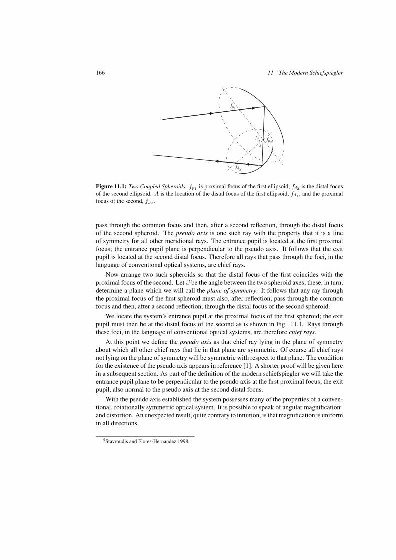
166 11 The Modern Schiefspiegler
Figure 11.1: Two Coupled Spheroids. fp1 is proximal focus of the first ellipsoid, fd2 is the distal focusof the second ellipsoid. A is the location of the distal focus of the first ellipsoid, fd1 , and the proximalfocus of the second, fp2 .
pass through the common focus and then, after a second reflection, through the distal focusof the second spheroid. The pseudo axis is one such ray with the property that it is a lineof symmetry for all other meridional rays. The entrance pupil is located at the first proximalfocus; the entrance pupil plane is perpendicular to the pseudo axis. It follows that the exitpupil is located at the second distal focus. Therefore all rays that pass through the foci, in thelanguage of conventional optical systems, are chief rays.
Now arrange two such spheroids so that the distal focus of the first coincides with theproximal focus of the second. Let β be the angle between the two spheroid axes; these, in turn,determine a plane which we will call the plane of symmetry. It follows that any ray throughthe proximal focus of the first spheroid must also, after reflection, pass through the commonfocus and then, after a second reflection, through the distal focus of the second spheroid.
We locate the system’s entrance pupil at the proximal focus of the first spheroid; the exitpupil must then be at the distal focus of the second as is shown in Fig. 11.1. Rays throughthese foci, in the language of conventional optical systems, are therefore chief rays.
At this point we define the pseudo axis as that chief ray lying in the plane of symmetryabout which all other chief rays that lie in that plane are symmetric. Of course all chief raysnot lying on the plane of symmetry will be symmetric with respect to that plane. The conditionfor the existence of the pseudo axis appears in reference [1]. A shorter proof will be given herein a subsequent section. As part of the definition of the modern schiefspiegler we will take theentrance pupil plane to be perpendicular to the pseudo axis at the first proximal focus; the exitpupil, also normal to the pseudo axis at the second distal focus.
With the pseudo axis established the system possesses many of the properties of a conven-tional, rotationally symmetric optical system. It is possible to speak of angular magnification5
and distortion. An unexpected result, quite contrary to intuition, is that magnification is uniformin all directions.
5Stavroudis and Flores-Hernandez 1998.
11.2 The Single Prolate Spheroid 167
This schiefspiegler differs from the earlier version in that it begins with an off-axis sys-tem, imposes conditions and restrictions, and analyzes the resulting structure. There are noapproximations; all calculations are exact.
In recognition of Anton Kutter’s earlier work I have called this system the modern schief-spiegler. Its elements are prolate spheroids, ellipsoids of revolution with the major axis of thegenerating ellipse as the axis of rotation on which lie the two foci. Earlier work along theselines can be found in reference [1].
11.2 The Single Prolate Spheroid
This is one of the conic sections of revolution that we had described in Chapters 2 and 4 wherewe choose a focus as a coordinate origin and the axis of rotation as the polar axis. This isshown in Fig. 11.2. As in previous chapters we refer to the focus at the coordinate origin as thespheroid’s proximal focus; the other as its distal focus. In Chapter 4 we applied generalized raytracing to get expressions for reflected rays and principal directions and principal curvaturesfor wavefronts associated with rays passing through the proximal and distal foci. As beforewe use the direction cosine vector, S = (ξ, η, ζ). Referring back to Chapter 7, for such a raywe found that the point of incidence is
(7.63) P = �(ξ, η, ζ),
where we obtained,
(7.64) � =r
1 − ε ζ,
the distance along the ray from the proximal focus to the point of incidence. Also from Chapter 7we have the unit normal vector to the reflecting surface at the point of incidence,
(7.65) N =1K (ξ, η, ζ − ε),
where,
(7.66) K2 = 1+ε2 −2ε ζ.
The cosine of the angle of incidence was found to be,
(7.68) cos i =1 − εζ
K .
From the ray tracing equation for reflection we have,
(7.70) S ′ =1K
((1 − ε2)ξ, (1 − ε2)η, (1 + ε2)ζ − 2 ε
).

168 11 The Modern Schiefspiegler
Figure 11.2: The Prolate Spheroid. A ray from the proximal focus is reflected by the spheroid and thenpasses through its distal focus. φ and φ′ are the angles the ray makes with the spheroid axis. ρ and ρ′
are the ray path lengths before and after reflection.
Figure 11.3: Illustrating the Prolate Spheroid. Show is a ray that passes through one focus, is reflectedby the ellipse, then passes through the second focus. ρ and ρ′ are the two distances from the point ofincidence to the two foci.
which when cast in scalar form becomes,
ξ ′ =1 − ε2
K ξ
η ′ =1 − ε2
K η
ζ ′ =1K [(1 + ε2)ζ − 2ε].
(11.1)
Finally, also from Eq. 7.64, the distance from the point of incidence to the distal focus is
(7.64) � ′ = �K2
1 − ε2.
These relationships are shown in Fig. 11.3
11.3 Coupled Spheroids
The principle behind the modern schiefspiegler the coupling of two prolate spheroids are sothat the distal focus of the first coincides with the proximal focus of the second. This we shallrefer to as the common focus. Here ε1 and r1 are the eccentricity and semi latus rectum of the
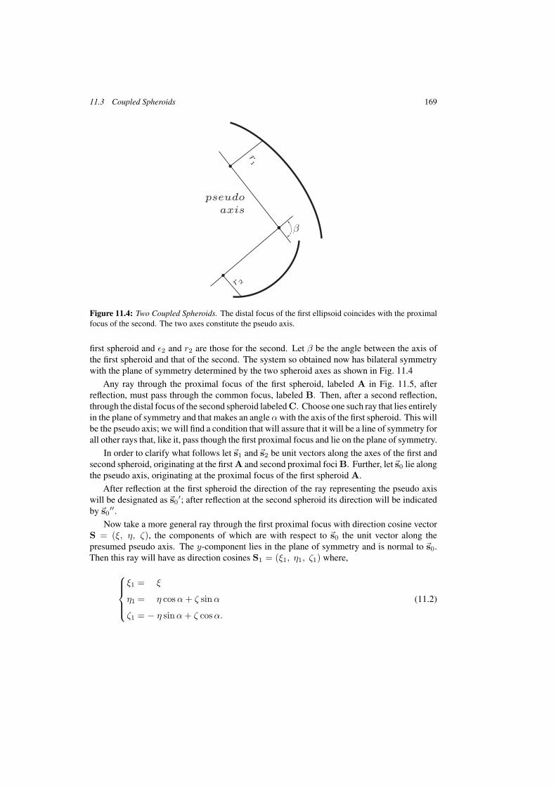
11.3 Coupled Spheroids 169
Figure 11.4: Two Coupled Spheroids. The distal focus of the first ellipsoid coincides with the proximalfocus of the second. The two axes constitute the pseudo axis.
first spheroid and ε2 and r2 are those for the second. Let β be the angle between the axis ofthe first spheroid and that of the second. The system so obtained now has bilateral symmetrywith the plane of symmetry determined by the two spheroid axes as shown in Fig. 11.4
Any ray through the proximal focus of the first spheroid, labeled A in Fig. 11.5, afterreflection, must pass through the common focus, labeled B. Then, after a second reflection,through the distal focus of the second spheroid labeled C. Choose one such ray that lies entirelyin the plane of symmetry and that makes an angle α with the axis of the first spheroid. This willbe the pseudo axis; we will find a condition that will assure that it will be a line of symmetry forall other rays that, like it, pass though the first proximal focus and lie on the plane of symmetry.
In order to clarify what follows let�s1 and�s2 be unit vectors along the axes of the first andsecond spheroid, originating at the first A and second proximal foci B. Further, let�s0 lie alongthe pseudo axis, originating at the proximal focus of the first spheroid A.
After reflection at the first spheroid the direction of the ray representing the pseudo axiswill be designated as �s0
′; after reflection at the second spheroid its direction will be indicatedby �s0
′′.Now take a more general ray through the first proximal focus with direction cosine vector
S = (ξ, η, ζ), the components of which are with respect to �s0 the unit vector along thepresumed pseudo axis. The y-component lies in the plane of symmetry and is normal to �s0.Then this ray will have as direction cosines S1 = (ξ1, η1, ζ1) where,
ξ1 = ξ
η1 = η cos α + ζ sin α
ζ1 = − η sin α + ζ cos α.
(11.2)
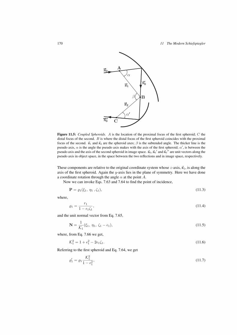
170 11 The Modern Schiefspiegler
Figure 11.5: Coupled Spheroids. A is the location of the proximal focus of the first spheroid; C thedistal focus of the second. B is where the distal focus of the first spheroid coincides with the proximalfocus of the second. �s1 and �s2 are the spheroid axes; β is the subtended angle. The thicker line is thepseudo axis, α is the angle the pseudo axis makes with the axis of the first spheroid; α′, is between thepseudo axis and the axis of the second spheroid in image space. �s0,�s0
′ and�s0′′ are unit vectors along the
pseudo axis in object space, in the space between the two reflections and in image space, respectively.
These components are relative to the original coordinate system whose z-axis,�s1, is along theaxis of the first spheroid. Again the y-axis lies in the plane of symmetry. Here we have donea coordinate rotation through the angle α at the point A.
Now we can invoke Eqs. 7.63 and 7.64 to find the point of incidence,
P = �1(ξ1, η1 , ζ1), (11.3)
where,
�1 =r1
1 − ε1ζ1, (11.4)
and the unit normal vector from Eq. 7.65,
N =1
K1(ξ1, η1, ζ1 − ε1), (11.5)
where, from Eq. 7.66 we get,
K21 = 1 + ε21 − 2ε1ζ1. (11.6)
Referring to the first spheroid and Eq. 7.64, we get
�′1 = �1
K21
1 − ε21, (11.7)

11.3 Coupled Spheroids 171
the distance from the point of incidence to the common focus, B.To Eq. 11.1 we apply the formulas for reflection given in Eq. 11.2 to get,
ξ′1 =
1 − ε21K1
ξ
η′1 =
1 − ε21K1
(η cos α + ζ sin α)
ζ ′1 =
1K1
[(1 + ε21)(−η sin α + ζ cos α) − 2ε1].
(11.8)
These components again need to be referred to�s1 and to the plane of symmetry.At the common focus we need to make another rotation of coordinates to a coordinate
system whose z-axis, indicated by�s2, is along the axis of the second spheroid. Recall that β isthe angle between the spheroid axes. Then the coordinate rotation, just as in Eq. 11.2, is givenby
ξ2 = ξ1′
η2 = η1′ cos β + ζ1
′ sin β
ζ2 = − η1′ sin β + ζ1
′ cos β,
(11.9)
where β is the angle between the two spheroid axes. Into Eq. 11.9 we substitute from Eq. 11.8to get the components of S′, now being referred to as �s2. These are,
ξ2 =1 − ε21
K1ξ
η2 =1
K1[−2ε1 sin β + Aη + Bζ]
ζ2 = − 1K1
[2ε1 cos β + Cη + Dζ],
(11.10)
where,
A = (1 − ε21) cos β cos α − (1 + ε21) sin β sin α
B = (1 − ε21) cos β sin α + (1 + ε21) sin β cos α
C = (1 − ε21) sin β cos α + (1 + ε21) cos β sin α
D = (1 − ε21) sin β sin α − (1 + ε21) cos β cos α
(11.11)
at point B. All this is shown in Fig. 11.5.We use again Eq. 7.66 to define,
K22 = 1 + ε22 − 2ε2 ζ2 (11.12)
172 11 The Modern Schiefspiegler
and use it and Eq. 11.6 to get,
K1K2 = (1 + ε22)K1 + 2ε2(2ε1 cos β + Cη + Dζ)
= (1 + ε21)(1 + ε22) + 4ε1ε2 cos β
+2η[ε1(1 + ε22) sin α + ε2C]
−2ζ[ε1(1 + ε22) cos α − ε2D].
(11.13)
By applying Eq. 7.64 we get the two relations
�2 =r2
1 − ε2ζ2=
r2K2
K2 + ε2(2ε1 cos β + Cη + Dζ),
�′2 = �2
K2
1 − ε22.
(11.14)
Finally we apply once again the reflection formulas in Eq. 11.1 to Eq. 11.10 and get S ′′
whose components are,
ξ′2 =
(1 − ε22)(1 − ε21)K1K2
ξ
η′2 =
1 − ε22K1K2
(−2ε1 sin β + Aη + Bζ)
ζ ′2 = − 1
K1K2[(1 + ε22)(2ε1 cos β + Cη + Dζ) + 2ε2K2
1]
= − 1K1K2
(2P + Qη − Rζ),
(11.15)
where,
P = ε2(1 + ε21) + ε1(1 + ε22) cos β
Q = 4ε1ε2 sin α + (1 + ε22)C
R = 4ε1ε2 cos α − (1 + ε22)D.
(11.16)
Equations 11.15 and 11.16 provides us with the direction cosines of this general ray at thedistal focus of the second spheroid in terms of a coordinate system whose z-axis lies along�s2,the axis of that second spheroid.
11.4 The Condition for the Pseudo Axis
We have tacitly assumed that the pseudo axis is that chief ray that makes an angle α with theaxis of the first spheroid. It makes sense to call α′ the angle that this same ray, in image space,makes with the axis of the second spheroid.

11.4 The Condition for the Pseudo Axis 173
Now let ξ = η = 0 so that ζ = 1. In what follows we signal this situation by a superiorbar as in S. Then Eq. 11.13 provides the angle α′ between the presumed pseudo axis and theaxis of the second spheroid. These are given by,{K1K2 sin α′ = (1 − ε22)(−2ε1 sin β + B)
K1K2 cos α′ = −2P + R,(11.17)
where, from Eq. 11.15,
K1K2 = (1 + ε21)(1 + ε22) + 4ε1ε2 cos β − 2[ε1(1 + ε22) cos α − ε2D]. (11.18)
Next we take a ray lying in the plane of symmetry that makes an angle θ with the presumedpseudo axis so that ξ = 0 and η = sin θ, ζ = cos θ. If θ ′ is the angle that this same ray makeswith the pseudo axis in image space then, from Eq. 11.15, we get,
sin(α′ + θ′) =
1 − ε22K1K2
(−2ε1 sin β + A sin θ + B cos θ)
cos(α′ + θ′) = − 1K1K2
(2P + Q sin θ − R cos θ).(11.19)
where, from Eq. 11.13,
K1K2 = (1 + ε21)(1 + ε22) + 4ε1ε2 cos β
+2[ε1(1 + ε22) sin α + ε2C] sin θ
−2[ε1(1 + ε22) cos α − ε2D] cos θ.
(11.20)
We use the identity
sin θ′ = sin(α′ + θ′) cos α′ − cos(α′ + θ′) sin α′ (11.21)
and Eqs. 11.17, 11.18 and 11.20 to get,
sin θ ′ =1
K1K2K1K2{2(BP − ε1R sin β)(1 − cos θ)
+[AR + BQ − 2(AP + ε1Q sin β)]} .
(11.22)
Recall that the condition for the pseudo axis is that it be a line of symmetry for all otherchief rays lying in the plane of symmetry. Consider θ ′ as a function of θ. Then for this to holdθ ′(−θ) = −θ ′(θ), so that θ ′ is an odd function of θ. Now look at the expression for the sineof θ ′ in Eq. 11.22. For it to be an odd function its numerator must be odd and its denominatormust be even. For the numerator to be odd the coefficient of 1 − cos θ must vanish. This givesus, with the aid of Eqs. 11.11 and 11.17, the following,
BP − ε1R sin β = [(1 − ε21) cos β sin α + (1 + ε21) sin β cos α]
×[ε2(1 + ε21) + ε1(1 + ε22) cos β] − ε1 sin β{4ε1ε2 cos α
−(1 + ε22)[(1 − ε21) sin β sin α − (1 + ε21) cos β cos α]}= (1 − ε21){[ε1(1 + ε22) + ε2(1 + ε21) cos β] sinα
+ε2(1 − ε21) sin β cos α} = 0.
(11.23)

174 11 The Modern Schiefspiegler
Consider now the expression for the factor in the denominator, K1K2, found in Eq. 11.20.(Note that the product K1K2 does not enter into this calculation because it does not depend onθ.) For the coefficient of sin θ to vanish
ε1(1 + ε22) sin α + ε2C = 0, (11.24)
which, on application of Eq. 11.11, yields,
tanα = − ε2(1 − ε21) sin β
ε1(1 + ε22) + ε2(1 + ε21) cos β. (11.25)
Note that the sum of the squares of numerator and denominator of the equation in Eq. 11.25is,
ε22(1 − ε21)2 sin2 β + [ε1(1 + ε22) + ε2(1 + ε21) cos β]2
= ε22(1 − ε21)2(1 − cos2 β) + ε21(1 + ε22)
2
+2ε1ε2(1 + ε21)(1 + ε22) cos β + ε22(1 + ε21) cos2 β
= ε21(1 + ε22)2 + ε22(1 − ε21)
2 + 2ε1ε2(1 + ε21)(1 + ε22) cos β
+ε22[(1 + ε21)2 − (1 − ε21)
2] cos2 β
= (1 + ε21ε22)(ε
21 + ε22) + 2ε1ε2[(1 + ε21ε
22) + (ε21 + ε22)] cos β
+4ε21ε22 cos2 β
= (1 + ε21ε22 + 2ε1ε2 cos β)(ε21 + ε22 + 2ε1ε2 cos β).
Now define,{p2 = 1 + ε21ε
22 + 2ε1ε2 cos β
q2 = ε21 + ε22 + 2ε1ε2 cos β,(11.26)
so that,{sin α = −ε2(1 − ε21) sin β/pq
cos α = [ε1(1 + ε22) + ε2(1 + ε21) cos β]/pq.(11.27)
This assures that the denominator of the expression for sin θ ′ will be an even function of θ.Substituting these expressions into Eq. 11.23 we see that that equation is satisfied also thusassuring that the numerator of sin θ ′ is an odd function. It follows that sin θ ′ is indeed an oddfunction and that Eq. 11.25 is indeed a condition for the system to possess a pseudo axis.
First of all note that, from Eq. 11.26,{p2 + q2 = (1 + ε21)(1 + ε22) + 4ε1ε2 cos β
p2 − q2 = (1 − ε21)(1 − ε22).(11.28)
Next, referring to Eq. 11.20, it can be shown that,
K1K2 = p2 + q2 − 2pq cos θ, (11.29)
11.5 Magnification and Distortion 175
so that,
K1K2 = (p − q)2. (11.30)
Now apply these results to Eq. 11.11 and get,
A = (1 − ε21)[ε2(1 + ε21) + ε1(1 + ε22) cos β]/pq
B = ε1(p2 + q2) sin β/pq
C = ε1(1 − ε21)(1 + ε22) sin β/pq
D = −[ε2(1 − ε21)2 + ε1(p2 + q2) cos β]/pq.
(11.31)
This and Eq. 11.17 yield up the following,
{sin α′ = ε1(1 − ε22) sin β/pq
cos α′ = [ε2(1 + ε21) + ε1(1 + ε22) cos β]/pq.(11.32)
The angle between the pseudo axis and the axis of the second ellipsoid is α′. The equationsfor α′ given in Eq. 11.32 can be obtained from the equations for α in Eq. 11.27 by interchanging′1′ and ′2′ and by changing the sign of β. This is tantamount to turning the system around.
11.5 Magnification and Distortion
The next step in this argument is the application of Eq. 11. 32 to Eq. 11.16 to get,
P = pq cos α′
Q = (p2 − q2) sin α′
R = (p2 + q2) cos α′.
(11.33)
These, together with Eqs. 11.31 and 11.32, when applied to Eq. 11.15, yield the vector S′′,whose components are,
ξ′2 = p2−q2
p2+q2−2pqζ ξ
η′2 = 1
p2+q2−2pqζ
{[ζ(p2 + q2) − 2pq
]cos α′
+η(p2 − q2) sin α′}
ζ ′2 = 1
p2+q2−2pqζ
{[ζ(p2 + q2) − 2pq
]sin α′
−η(p2 − q2) cos α′}
,
(11.34)
which, as before, refer to �s2, the vector along the axis of the second spheroid.
176 11 The Modern Schiefspiegler
A final rotation of these vector components, through the angle α, as done in Eq. 11.2, givesus S′′ = (ξ∗, η∗, ζ∗), where,
ξ∗ =p2 − q2
p2 + q2 − 2pqζξ
η∗ =p2 − q2
p2 + q2 − 2pqζη
ζ∗ =ζ(p2 + q2) − 2pq
p2 + q2 − 2pqζ.
(11.35)
These components are now referred to �s0′′, the unit vector along the pseudo axis in image
space. This final rotation takes place at point C. See Fig. 11.5.We can see from Eq. 11.35 that the pseudo axis, in image space, is indeed an axis of
symmetry, not only for those chief rays lying in the plane of symmetry, but also for all chiefrays. From this it follows that the attributes of chief rays that lie in the plane of symmetry willapply to all chief rays. So, with no loss of generality we find expressions for magnificationand distortion for those rays lying in the plane of symmetry, confident that they will be validfor all chief rays.
So once again let ξ = 0 and let η = sin θ, ζ = cos θ ; then η∗ = sin θ′ and ζ∗ = cos θ′.From Eq. 11.35 we can get,
tan θ ′ =(p2 − q2) sin θ
(p2 + q2) cos θ − 2pq= M(θ) tan θ, (11.36)
where,
M(θ) =(p2 − q2) cos θ
(p2 + q2) cos θ − 2pq. (11.37)
The magnification of the system must then be M(0),
M(0) = M =p + q
p − q, (11.38)
so that distortion is,
D(θ) = M(θ) − M(0)
=p + q
p − q
2pq(1 − cos θ)(p2 + q2) cos θ − 2pq
.(11.39)
Distortion as a fraction of magnification then must be,
D(θ) =2pq(1 − cos θ)
(p2 + q2) cos θ − 2pq. (11.40)
Now return to Eq. 11.38 and solve for p to get,
p =M + 1M − 1
q. (11.41)
11.6 Conclusion 177
When this is substituted into Eq. 11.40 we get
D(θ) =(M2 − 1)(1 − cos θ)
(M2 + 1) cos θ − (M2 − 1), (11.42)
which shows that distortion depends only on the system’s angular magnification.
11.6 Conclusion
The modern schiefspiegler is an unusual system. The derivation of the condition for theexistence of the pseudo axis reveals its unique properties. The good news, as shown in Eq. 11.35,is that its chief rays behave like chief rays in a rotationally symmetric system; that magnificationis uniform in all directions. The bad news is that, once magnification is established, distortionis a fixed function of θ.
All of the results presented here can be extended to hyperboloids of two sheets by setting thevalue of the eccentricity (ε) to a value greater than unity or, in the case of telecentric systems,equal to unity. Moreover, by changing the sign of ε in Eq. 7.64, the roles of the proximaland distal foci are interchanged. However, all of our numerical work has been with prolatespheroids with the proximal and distal foci in their usual order.
A modest but comprehensive literature pertaining to the first-order properties of the systemswithout symmetry and their aberrations exists, beginning with a chapter in Kutter’s book.Sands’6 development of an aberration theory for what he calls plane symmetric systems anddouble-plane symmetric systems is certainly germane as is a more general work by Buchdahl.7
The more modern and monumental work of Stone and Forbes,8 which appeared in the latertwentieth century, will certainly play an important role in the development of the schiefspiegler.
6Sands 1972, 1973a, and Sands 1973b.7Buchdahl 1972.8Stone and Forbes 1992a, Stone and Forbes 1992c, Stone and Forbes 1992d, and Stone and Forbes 1992e.

The Mathematics of Geometrical and Physical Optics: The k-function and its Ramifications. O.N. StavroudisCopyright c© 2006 WILEY-VCH Verlag GmbH & Co. KGaA, WeinheimISBN: 3-527-40448-1
12 The Cartesian Oval and its Kin
Cartesian ovals are a class of refracting surfaces that image perfectly an object point into animage point. The first to find its algebraic formula was Descartes, though it is said that Keplerhad obtained a numeric solution as early as 1602. Descartes was the first of a long line ofinvestigators that had derived its formula independently, among whom was Maxwell; indeed,it is sometimes referred to as the Maxwellian oval.
It used to be that a new derivation was announced about every ten years giving us knowl-edgeable folk an opportunity to display our erudition,1 but nowadays there is little interest ininvestigations of this kind.
There are two approaches to finding the equation for this kind of surface. One, which we willapply here, uses elementary algebra and relies on the fact that the optical path length, throughany optical system, between two conjugate points, is constant. The other uses the refractionequation and the unit normal vector to the desired surface to find a partial differential equationwhose solution is the appropriate formula.
The surface must be rotationally symmetric with the axis of symmetry being the lineconnecting the two conjugate points. Its equation is a quartic polynomial. However wheneither the object point or its image point is at infinity the equation degenerates into either aprolate spheroid or a hyperboloid of two sheets. When the surface is forced into the shape ofa sphere, the two conjugate points become the aplanatic points of the sphere which we hadalready encountered in Chapter 9.
12.1 The Algebraic Method
Suppose a point on the required surface has the coordinates, P = (x, y, z), that the coordinatesof the object point are P0 = (0, 0, −t) = −tZ and that those of the image point areP1 = (0, 0, t1) = t1Z, where the z-axis is to be the line connecting P0 and P1. The unitvector Z, of course, lies along the z-axis. Let the coordinate origin lie on this line at the pointwhere it intersects the desired surface as is shown in Fig. 12.1. Then the distance d from theobject point to P on the surface is,
d2 = (P + tZ)2 = (x, y, z + t)2 = P2 + 2tz + t2, (12.1)
and the distance d1 from P to the image point is,
d21 = (P − t1Z)2 = (x, y, z − t1)2 = P2 − 2t1z + t21, (12.2)
1See, for example, O’Connell 1998.
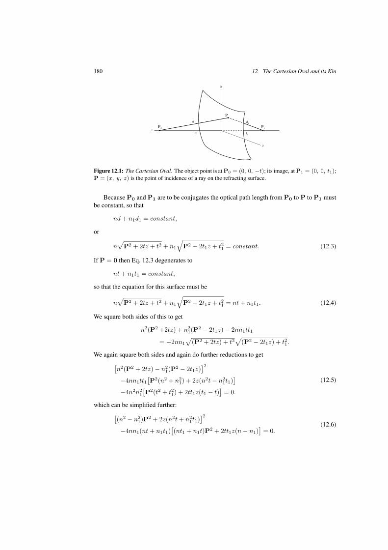
180 12 The Cartesian Oval and its Kin
Figure 12.1: The Cartesian Oval. The object point is at P0 = (0, 0, −t); its image, at P1 = (0, 0, t1);P = (x, y, z) is the point of incidence of a ray on the refracting surface.
Because P0 and P1 are to be conjugates the optical path length from P0 to P to P1 mustbe constant, so that
nd + n1d1 = constant,
or
n√
P2 + 2tz + t2 + n1
√P2 − 2t1z + t21 = constant. (12.3)
If P = 0 then Eq. 12.3 degenerates to
nt + n1t1 = constant,
so that the equation for this surface must be
n√
P2 + 2tz + t2 + n1
√P2 − 2t1z + t21 = nt + n1t1. (12.4)
We square both sides of this to get
n2(P2 +2tz) + n21(P
2 − 2t1z) − 2nn1tt1
= −2nn1√
(P2 + 2tz) + t2√
(P2 − 2t1z) + t21.
We again square both sides and again do further reductions to get[n2(P2 + 2tz) − n2
1(P2 − 2t1z)
]2−4nn1tt1
[P2(n2 + n2
1) + 2z(n2t − n21t1)
]−4n2n2
1[P2(t2 + t21) + 2tt1z(t1 − t)
]= 0.
(12.5)
which can be simplified further:[(n2 − n2
1)P2 + 2z(n2t + n2
1t1)]2
−4nn1(nt + n1t1)[(nt1 + n1t)P2 + 2tt1z(n − n1)
]= 0.
(12.6)
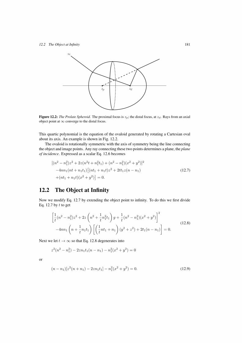
12.2 The Object at Infinity 181
Figure 12.2: The Prolate Spheroid. The proximal focus is zp; the distal focus, at zd. Rays from an axialobject point at ∞ converge to the distal focus.
This quartic polynomial is the equation of the ovaloid generated by rotating a Cartesian ovalabout its axis. An example is shown in Fig. 12.2.
The ovaloid is rotationally symmetric with the axis of symmetry being the line connectingthe object and image points. Any ray connecting these two points determines a plane, the planeof incidence. Expressed as a scalar Eq. 12.6 becomes
[(n2 − n21)z
2 + 2z(n2t + n21t1) + (n2 − n2
1)(x2 + y2)]2
−4nn1(nt + n1t1)[(nt1 + n1t)z2 + 2tt1z(n − n1)
+(nt1 + n1t)(x2 + y2)]
= 0.
(12.7)
12.2 The Object at Infinity
Now we modify Eq. 12.7 by extending the object point to infinity. To do this we first divideEq. 12.7 by t to get
[1t(n2 − n2
1)z2 + 2z
(n2 +
1tn2
1t1
)g +
1t(n2 − n2
1)(x2 + y2)
]2
−4nn1
(n +
1tn1t1
)[(1tnt1 + n1
)(y2 + z2) + 2t1(n − n1)
]= 0.
(12.8)
Next we let t → ∞ so that Eq. 12.8 degenerates into
z2(n2 − n21) − 2zn1t1(n − n1) − n2
1(x2 + y2) = 0
or
(n − n1)[z2(n + n1) − 2zn1t1] − n21(x
2 + y2) = 0. (12.9)
182 12 The Cartesian Oval and its Kin
This we multiply by n + n1 and complete the square to get
(n − n1)[z(n + n1) − n1t1]2 − n21(x
2 + y2)(n + n1) = (n − n1)n21t
21, (12.10)
a quadratic polynomial that clearly represents a conic section of revolution.
1B2
(z − n1t1
n + n1
)2
+1
A2 (x2 + y2) = 1, (12.11)
where
A2 =n2
1
(n1 + n)2t21
B2 =n1 − n
n1 + nt21.
(12.12)
12.3 The Prolate Spheroid
First suppose that n1 > n. Then Eq. 12.11 can be interpreted as the equation of a prolatespheroid (an ellipsoid generated by revolving an ellipse about its major axis) with its center ofsymmetry at zc = A and whose eccentricity, from the standard formula2 is
ε =
√1 − B2
A2 =
√1 − n2
1 − n2
n21
=n
n1< 1. (12.13)
By setting x = y = 0 in Eq. 12.11 we find the intercepts with the z-axis to be z = 0 andz = 2a, just as they should.
The distance from the center A to each of the two foci equals εA = nt1/(n1 − n) so thattheir coordinates are
zp = A(1 − ε) =
n1t1n1 + n
(1 − n
n1) = t1
n1 − n
n1 + n
zd = A(1 + ε) =n1t1
n1 + n(1 +
n
n1) = t1,
(12.14)
where zp is the proximal focus and zd is the distal focus. This shows that the optical focusof the refracting prolate spheroid is at the spheroid’s distal focus, the focus further from thevertex. Here the use of the word focus for two different concepts is indeed confusing.
Using a standard formula, we find the latus rectum to be,
latus rectum = 2B2
A= 2t1
n1 + n
n1. (12.15)
This is all shown in Fig. 12.3.2The literature is indeed sparse. The Cartesian oval appears as an exercise in Buchdahl 1970, p. 310. Luneburg
1966, pp. 129–138 gives a detailed account (with part of which I disagree) and Stavroudis 1972, pp. 97–100 (in whichI perpetuate Luneburg’s incorrect methods). There is also Herzberger 1958, Chapter 17.

12.4 The Hyperboloid of Two Sheets 183
Figure 12.3: Showing the ellipse. zp and zd are the proximal and distal foci; A represents the center.The vertical line through zp is the semi latus rectum.
12.4 The Hyperboloid of Two Sheets
Now suppose that n > n1 so that Eq. 12.11 becomes,
− 1B2
(z − n1t1
n + n1
)2
+1
A2 (x2 + y2) = 1, (12.16)
where,
A2 =n2
1
(n1 + n)2t21
B2 =n − n1
n1 + nt21,
(12.17)
so the Cartesian oval degenerates into a hyperboloid of two sheets with its center of symmetryat zc = −A and with its z-intercepts at z = 0 and at z = −2A.
Again we find the eccentricity to be,
ε =
√1 +
B2
A2 =
√1 +
n2 − n21
n21
=n
n1> 1. (12.18)
As in the case of the spheroid, the two foci of the hyperboloid lie a distance εA on either sideof the center of symmetry, zc = −A so that their coordinates are,
zp = −A(1 − ε) = − n1t1
n + n1
(1 − n
n1
)= t1
n − n1
n + n1
zd = −A(1 + ε) = − n1t1n + n1
(1 +
n
n1
)= −t1.
(12.19)
This is analogous to the case of the prolate spheroid. To avoid unnecessary confusion we retainthe notation for the proximal focus, zp, the focus nearest the coordinate origin, and the distalfocus, zd, the more remote focus, which in this case has a negative z-coordinate. The distalfocus, as in the case of the prolate spheroid, is the image of the infinite object point and isvirtual. The latus rectum is the same as for the spheroid and is given by Eq. 12.15. This is allillustrated in Fig. 12.4.

184 12 The Cartesian Oval and its Kin
Figure 12.4: The Hyperboloid of Two Sheets. The proximal focus is zp; the distal focus, at zd the locationof the virtual image of the axial object point at ∞.
12.5 Other Surfaces that Make Perfect Images
An interesting experiment relates to Eq. 12.6 which contains two factors each enclosed inbrackets. Suppose we chose t and t1 in such a way that these factors were equal and thereforethe equation would split into the product of two quadratics. Let k be some factor yet to bedetermined and let{
n2 + n21 = k(n1t + nt1)
n2t + n21t1 = ktt1(n − n1),
(12.20)
a pair of simultaneous equations that have two sets of solutions
t = −n1/k, t1 = nk (12.21)
and
t = −(n + n1)/k, t1 = (n + n1)/k. (12.22)
Look at the first of these solutions, Eq. 12.21. First of all notice that nt + n1t1 = 0 sothat the optical path from object point to image point is zero and that the first term of Eq. 12.6becomes
(n2 − n21)P
2 − 2nn1z(n − n1)/k = 0
which can be rearranged into
(z − nn1
k(n + n1)
)2
+ x2 + y2 =(
nn1
k(n + n1)
)2
(12.23)
the equation of a sphere with z-intercepts at z = 0 and atz = 2nn1/k(n + n1) and with a radius r = nn1/k(n + n1) so that
k =nn1
r(n + n1). (12.24)

12.5 Other Surfaces that Make Perfect Images 185
Figure 12.5: Showing the Aplanatic Points and Surfaces of a sphere. Rays focused on point z1 in objectspace are refracted to focus on point z2 in image space. z is the common center.
When this value of k is substituted back into Eq. 12.21 we get
t = −r(1 + n1/n), t1 = r(1 + n/n1). (12.25)
These represent distances to an object point and its image point that are imaged perfectly bythe refracting sphere. These are the aplanatic points of the sphere and are shown in Fig. 12.5.
We can go further. Because the sphere is centrally symmetric two spheres can be generatedby rotating the aplanatic points about the sphere’s center. This generates a pair of spheres thatare perfect images of one another. These are referred to as the aplanatic surfaces of a sphere.This is also illustrated in Fig. 12.5.
In days long past, before the advent of the computer, the aplanatic points and the aplanaticsurfaces were used to trace rays graphically. Using only a straight edge and a compass,meridianal rays could be traced directly on the layout of a lens design, not with great accuracybut adequate for a quick and rough evaluation.
Now we return to Eq. 12.22 the other solution of the equations given in Eq. 12.20. As beforewe substitute these expressions into the equation for the Cartesian oval given in Eq. 12.6. Theresult is(
P2 − 2zn + n1
k
)[(P2 − 2z
n + n1
k
)+ 4
nn1
k2
]= 0. (12.26)
We look at each quadratic factor separately. The left factor becomes
(z − n + n1
k
)2
+ x2 + y2 =(
n + n1
k
)2
186 12 The Cartesian Oval and its Kin
another sphere that passes through the origin with radius r = (n + n1)/k so in this case
k =n + n1
r. (12.27)
When this is substituted into Eq. 12.22 we get
t = −r, t1 = r (12.28)
a statement of the unremarkable fact that the center of a sphere is its own perfect image.The right hand factor of Eq. 12.26 is(
P2 − 2zn + n1
k
)+ 4
nn1
k2 = 0
which becomes
x2 + y2 + (z − 2n
k)(z − 2n1
k) = 0, (12.29)
the equation of an ovaloid with intercepts at z = 2n/k and at z = 2n1/k.This concludes this shortest of chapters on the Cartesian oval. Unfortunately it seems to
have no real applications except as a magnifying glass where the narrow end of the oval is cutoff normal to the axis at the location of the image point and polished as a plane surface. Thenwhen the plane surface is placed on a sheet of paper on which there is writing or some sort ofdiagram, a magnified virtual image is formed.
But it does give us a chance to display our erudition when the Cartesian oval is againrediscovered and republished.

The Mathematics of Geometrical and Physical Optics: The k-function and its Ramifications. O.N. StavroudisCopyright c© 2006 WILEY-VCH Verlag GmbH & Co. KGaA, WeinheimISBN: 3-527-40448-1
13 The Pseudo Maxwell Equations
The first nine chapters are about Fermat’s principle and its consequences. From this medievalrelic we derived the eikonal equation and obtained its general solution in which the k-functionfirst appeared as its arbitrary function. In Chapter 10 we parted from our preoccupation withgeometrical optics and applied our previous results to the Maxwell equations for homogeneous,isotropic media. This lead us to a solution of the Maxwell equations in terms of the k-function.
We have demonstrated the power and the depth of Fermat’s principle. In this chapter wespeculate. Is there a more subtile relationship between the Maxwell equations and the axiomsof geometrical optics? In this speculation we will return to the optics of inhomogeneous mediaand refer to our previous results in Chapters 1, 2 and 7. We will also write the Maxwellequations once again in terms of the arc length parameter s instead of the time parameter t.
13.1 Maxwell Equations for Inhomogeneous Media
A more general version than that used in Chapter 10 includes ε as a function of position whileµ is assumed to be a constant.1
∇ × E = −1
c
∂B∂t
∇ · B = 0 B = µH
∇ × H =1c
∂D∂t
∇ · D = 0 D = εE.
(13.1)
However we need to make a change of variables from the time parameter t to the arc lengthparameter s as was done in Chapter 10
(10.2)∂
∂t=
ds
dt
∂
∂s= v
∂
∂s=
c
n
∂
∂s.
The assumption that µ is constant leads to fatal inconsistencies; we must take it to be a functionof position as is ε. To be consistent with reality we can assume that it is a slowly varyingfunction of s.
∇ × E = −
õ
ε
∂H∂s
− µs
nH µ∇ · H + ∇µ · H = 0
∇ × H =√
ε
µ
∂E∂s
+εs
nE ε∇ · E + ∇ε · E = 0
(13.2)
1Borne and Wolf 1999, Chapter I.

188 13 The Pseudo Maxwell Equations
13.2 The Frenet-Serret Equations
Now refer back to the vector trihedron in Chapter 2 and the relationship between t, n and band the Frenet-Serret equations expressed in terms of the directional derivative
(2.12)
t = n × b, ts = (t · ∇)t =1ρn,
n = b × t, ns = (t · ∇)n = −1ρt +
1τb,
b = t × n, bs = (t · ∇)b = −1τn.
Let a train of wavefronts in an inhomogeneous medium be represented in the usual wayby the vector function W(v, w, s). But the medium is not homogeneous so the results ofChapter 7 cannot apply. On the other hand the results of Chapter 1 do indeed apply and so wewill make use of Eq. 1.29
(1.29d
ds(nPs) = ∇n,
and its equivalent expanded form
(1.30) nPss+(∇n·Ps)Ps = ∇n.
The results of Chapter 2 also apply and so we will make use of those forms of the ray equation,given in Eqs. 2.50 and 2.52, that involves the unit tangent vector t and the unit normal vector n
(2.50)n
ρn+(∇n·t)t = ∇n.
and its equivalent
(2.52)1ρn =
1nt×(∇n×t),
as well as Eq. 2.51 that relates to the unit binormal vector b,
(2.51) ∇n·b = 0.
We will also need
∇n · n =n
ρ, (13.3)
also from Eq. 2.50.
13.3 Initial Calculations
These, Eqs. 2.50, 2.51 and 2.52, all relate to a ray, necessarily normal to the wavefront, as wellas its vector trihedron, t, n and b. We have seen in Chapter 4 that the surface parameters can
13.3 Initial Calculations 189
always be transformed according to a strict set of rules. Now we assume that this has alreadybeen done; that Wv is in the direction of n and that Ww is in the direction of b. Through eachpoint on the wavefront pass two of these lines of curvature that are perpendicular to each other.Moreover, since N is equal to t these parametric curves are geodesics as shown in Chapter 4.
The notation is indeed confusing. The ray’s unit tangent vector t is also the unit normalvector N to the wavefront while n and b are normal to the ray and tangent to the wavefrontsurface. In an attempt to make things clearer we distinguish the two vector trihedrals associatedwith the two families of parametric curves by superscripts, (v) and (w); thus
tv = n, nv = t; (13.4)
and
tw = b, nw = t; (13.5)
so that
bv = tv × nv = n × t = −b,
bw = tw × nw = b × t = n.(13.6)
Recall that in Chapter 7 we had applied the Frenet-Serret equations to the N, P, Q coor-dinate system to get the equations of generalized ray tracing. We do the same thing here to get,eventually, the expressions that I have called the pseudo Maxwell equations.
To each of these families of curves we next apply the Frenet-Serret equations, Eq. 2.12.For the v-curves we get
(tv · ∇)tv =1ρv
nv
(tv · ∇)nv = − 1ρv
tv +1τv
bv
(tv · ∇)bv = − 1τv
nv.
(13.7)
When we apply Eqs. 13.4 and 13.5 to these we get
(n · ∇)n =1ρv
t
(n · ∇)t = − 1ρv
n − 1τv
b
−(n · ∇)b = − 1τv
t,
(13.8)
190 13 The Pseudo Maxwell Equations
where 1/ρv is the curvature and 1/τv the torsion of the family of v-curves. We do exactly thesame thing for the w-curves to get
(b · ∇)b =1ρw
t
(b · ∇)t = − 1ρw
b +1τw
n
(b · ∇)n = − 1τw
t,
(13.9)
where, naturally, 1/ρw is the curvature and 1/τw the torsion of each member of the family ofw-curves.
Now refer back to Chapter 7 and the following equation
(7.34)1σ
= − 1τv
=1τw
.
Although it had been applied to the expression for wavefronts in homogeneous, isotropic mediaits derivation was not limited to that case and can be applied to this situation. By applyingEq. 7.34 to Eqs. 13.8 and 13.9 we get
(n · ∇)n =1ρv
t
(n · ∇)t = − 1ρv
n +1σb
(n · ∇)b = − 1σt,
(13.10)
and
(b · ∇)b =1ρw
t
(b · ∇)t = − 1ρw
b +1σn
(b · ∇)n = − 1σt.
(13.11)
13.4 Divergence and Curl
In what follows we will need the following vector identities from the Appendix
(A.12) ∇(E·F) = (E·∇)F+(F·∇)E+E×(∇×F)+F×(∇×E),
(A.13) ∇·(E×F) = F·(∇×E)−E·(∇×F),
(A.14) ∇×(E×F) = (F·∇)E−(E·∇)F+E(∇·F)−F(∇·E).
In particular, we will need the fact that if A2 = constant then, from Eq. A.7
(A.20) (A·∇)A = −A×(∇×A).

13.4 Divergence and Curl 191
Look first at the divergence of t, in which we use repeatedly the vector products fromEqs. A.12 to A.14.
∇ · t = ∇ · (n × b) = b · (∇ × n) − n · (∇ × b)
= (t × n) · (∇ × n) − (b × t) · (∇ × b)
= t · [n × (∇ × n) + b × (∇ × b)],
to which we apply Eq. A.20, and get
∇ · t = −t · [(n · ∇)n + (b · ∇)b],
which leads at once to, using Eqs. 13.10 and 13.11,
∇ · t = −t ·[
1ρv
t +1ρw
t]
= −(
1ρv
+1ρw
), (13.12)
a result obtained by Kline and Kay2 using essentially the same methods. By using this samestrategy we can also obtain
∇ · n = ∇ · (b × t) = t · (∇ × b) − b × (∇ × t)
= (n × b) · (∇ × b) − (t × n) · (∇ × t)
= n · [b × (∇ × b) + t × (∇ × t)]
= −n · [(b · ∇)b + (t · ∇)t]
= −n ·[
1ρw
t +1ρn]
,
resulting in
∇ · n = −1ρ. (13.13)
Also
∇ · b = ∇ · (t × n) = n · (∇ × t) − t × (∇ × n)
= (b × t) · (∇ × t) − (n × b) · (∇ × n)
= b · [t × (∇ × t) + n × (∇ × n)]
= −b · [(t · ∇)t + (n · ∇)n]
= −b ·[1ρn +
1ρv
t]
,
so that
∇ · b = 0. (13.14)
2Kline and Kay 1965, pp. 184–186.
192 13 The Pseudo Maxwell Equations
Next we return to the calculation of the curls of the three vectors that comprise the vectortrihedron. In what follows we use Eqs. A.6, 7.34, 13.10 and 13.11 to get
∇ × t = ∇ × (n × b)
= (b · ∇)n − (n · ∇)b + (∇ · b)n − (∇ · n)b
= 1ρb,
(13.15)
∇ × n = ∇ × (b × t)
= (t · ∇)b − (b · ∇)t + (∇ · t)b − (∇ · b)t
= − ( 1σ + 1
τ
)n − 1
ρvb,
(13.16)
and
∇ × b = ∇ × (t × n)
= (n · ∇)t − (t · ∇)n + (∇ · n)t − (∇ · t)n= 1
ρwn +
( 1σ − 1
τ
)b.
(13.17)
13.5 Establishing the Relationship
We now write the electric field vector, e, and the magnetic field vector, h, as linear combinationsof n and b{
e = αn + β b
h = −β n + αb,(13.18)
so that e · h = 0 and e × h = (α2 + β2)t. We use the results of the previous section tocalculate the curls, divergences and derivatives of e and h for substitution into Eqs. 13.2. Firstthe divergences. From Eq. 13.2
ε ∇ · e + ∇ε · e = 0
= ε[α(∇ · n) + β(∇ · b) + (∇α · n) + (∇β · b)
]+ ∇ε · (αn + βb)
= −αε/ρ + ε(n · ∇)α + ε(b · ∇)β + α(n · ∇)ε + β(b · ∇)e,
which leads to
αε/ρ = (n · ∇)(εα) + (b · ∇)(εβ). (13.19)
In exactly the same way, also from Eq. 13.2, we get the divergence of h
βµ/ρ = (n · ∇)(µβ) − (b · ∇)(µα). (13.20)

13.5 Establishing the Relationship 193
The curls of e and h come next. Here we use Eqs. 13.16, 13.17 and 13.18 to get
∇× e = ∇ × (αn + βb)
= α(∇ × n) + β(∇ × b) + (∇α × n) + (∇β × b)
= α
[−
(1σ
+1τ
)n − 1
ρvb]
+β
ρwn +
(1σ
+1τ
)b
+(∇α · t)b − (∇α · b)t + (∇β · n)t − (∇β · t)n
= t [−(∇α · b) + (∇β · n)] + n[−α
(1σ
+1τ
)+
β
ρw− βs
]
+b[− α
ρv+ β
(1σ
− 1τ
)+ αs
],
(13.21)
and
∇× h = ∇ × (−βn + αb)
= −β(∇ × n) + α(∇ × b) − (∇β × n) + (∇α × b)
= −β
[−
(1τ
+1σ
)n − 1
ρvb]
+ α
[1ρw
n +(
1σ
− 1τ
)b]
−βsb + (∇β · b)t + (∇α · n)t − αsn
= t [(∇β · b) + (∇α · n)] + n[β
(1σ
+1τ
)+
α
ρw− αs
]
+b[
β
ρv+ α
(1σ
− 1τ
)− βs
].
(13.22)
The derivatives are much simpler.
es = (αn + β b)s = αns + β bs + αs n + βs b
= α
(−1
ρt +
1τb)
+ β
(−1
τn)
+ αs n + βs b
= −α
ρt +
(αs − β
τ
)n +
(βs +
α
τ
)b,
(13.23)
and
hs = (−β n + αb)s = −β ns + αbs − βs n + αs b
= −β
(−1
ρt +
1τb)
+ α
(−1
τn)
− βs n + αs b
=β
ρt −
(βs +
α
τ
)n +
(αs − β
τ
)b.
(13.24)
Eq. 13.19 becomes
αε/ρ = (n · ∇)(αε) + (b · ∇)(βε)
= ε[∇α · n + ∇β · b] + α(∇ε · n) + β(∇ε · b)(13.25)
194 13 The Pseudo Maxwell Equations
and Eq. 13.20 turns into
βµ/ρ = (n · ∇)(βµ) + (b · ∇)(αµ)
= µ[∇β · n − ∇α · b] + β(∇µ · n) − α(∇µ · b).(13.26)
We substitute the expressions in Eqs. 13.21 and 13.24 back into Eqs. 13.2 to get
∇ × e = t [−(∇α · b) + (∇β · n)] + n[−α
(1σ
+1τ
)+
β
ρw− βs
]
+b[− α
ρv+ β
(1σ
− 1τ
)+ αs
]
= −√
µ
ε
[β
ρt −
(βs +
α
τ
)n +
(αs − β
τ
)b]
− µs
n(−βn + αb),
which leads to
t[−(∇α · b) + (∇β · n) +
β
ρ
õ
ε
]
+n[−α
(1σ
+1τ
)+
β
ρw− βs −
õ
ε
(βs +
α
τ
)− β
µs
n
]
+b[β
(1σ
− 1τ
)− α
ρv+ αs +
õ
ε
(αs − β
τ
)+ α
µs
n
]= 0.
(13.27)
In exactly the same way we use Eqs. 13.22 and 13.23 to get
∇ × h = t[(∇α · n) + (∇β · b)
]+ n
[β
(1σ
+1τ
)+
α
ρw− αs
]
+b[
β
ρv+ α
(1σ
− 1τ
)− βs
]
=√
ε
µ
[−α
ρt +
(αs − β
τ
)n +
(βs +
α
τ
)b]
+εs
n(αn + βb),
which results in
t[∇α · n + ∇β · b +
α
ρ
√ε
µ
]
+n[β
(1σ
+1τ
)+
α
ρw− αs −
√ε
µ
(αs − β
τ
)−α
εs
n
]
+b[α
(1σ
− 1τ
)+
β
ρv− βs −
√ε
µ
(βs +
α
τ
)− β
εs
n
]= 0.
(13.28)
From Eqs. 13.27 and 13.28 we get six scalar equations. Since each is a linear combinationof the three orthogonal vectors t, n and b set equal to zero the coefficients must also vanish
13.5 Establishing the Relationship 195
resulting in
a) − (∇α · b) + (∇β · n) +β
ρ
õ
ε= 0,
b) − α
σ+
β
ρw−
(βs +
α
τ
) (1 +
õ
ε
)− β
µs
n= 0,
c)β
σ− α
ρv+
(αs − β
τ
) (1 +
õ
ε
)+ α
µs
n= 0,
d) ∇α · n + ∇β · b +α
ρ
√ε
µ= 0,
e)β
σ+
α
ρw−
(αs − β
τ
) (1 +
√ε
µ
)− α
εs
n= 0,
f)α
σ+
β
ρv−
(βs +
α
τ
) (1 +
√ε
µ
)− β
εs
n= 0.
(13.29)
Two more scalar equations come from Eqs. 13.25 and 13.26
g) αε/ρ = ε[∇α · n + ∇β · b] + α(∇ε · n) + β(∇ε · b),
h) βµ/ρ = µ[−∇α · b + ∇β · n] − α(∇µ · b) + β(∇µ · n).(13.30)
Finally from Eqs. 2.56, 2.57 and 13.3 we get
∇n · b =12
[õ
ε(∇ε · b) +
√ε
µ(∇µ · b)
]= 0,
∇n · n =12
[õ
ε(∇ε · n) +
√ε
µ(∇µ · n)
]= n/ρ,
which leads to
i) µ(∇ε · b) + ε(∇µ · b) = 0,
j) µ(∇ε · n) + ε(∇µ · n) = 2n2/ρ.(13.31)
Now refer back to Eq. 13.29 and subtract e from c to get
α(∇ · t) +1n
(√
ε +√
µ)2(
αs − β
τ
)+
α
n(εs + µs) = 0, (13.32)
as well as, by adding b and f ,
−β(∇ · t) − 1n
(√
ε +√
µ)2(βs +
α
τ
)− β
n(εs + µs) = 0. (13.33)
Now multiply Eq. 13.32 by β and Eq. 13.33 by α then add. The result after some reduction is
αsβ − αβs =1τ
(α2 + β2). (13.34)
196 13 The Pseudo Maxwell Equations
Note that
αsβ − αβs
α2 + β2 =d
dsarctan
(α
β
)=
1τ
,
so that
α = β tanU (13.35)
where
U =∫
ds
τ. (13.36)
Next we substitute Eq. 13.35 into Eq. 13.32 and get
tanU
[β(∇ · t) +
β
n(εs + µs)
]+
1n
(√
ε +√
µ)2(
αs − β
τ
)= 0 (13.37)
and at the same time we make the same substitution into Eq. 13.33 resulting in
−[β(∇ · t) +
β
n(εs + µs)
]− 1
n(√
ε +√
µ)2(
βs − β
τtanU
)= 0. (13.38)
By multiplying Eq. 13.38 by tanU and adding to Eq. 13.37 yields, after some reduction
τ(αs − βs tanU) = β(1 + tan2 U)
or
β = τ cos U(αs cos U − βs sin U) (13.39)

The Mathematics of Geometrical and Physical Optics: The k-function and its Ramifications. O.N. StavroudisCopyright c© 2006 WILEY-VCH Verlag GmbH & Co. KGaA, WeinheimISBN: 3-527-40448-1
14 The Perfect Lenses of Gauss and Maxwell
Like so many other myths in geometrical optics, a prefect lens is so rare as to be almostnonexistent. It should be rotationally symmetric and be able to image certain points in objectspace perfectly in image space. Examples of real prefect lenses are the Maxwell’s fish eye, thatwas discussed in Chapters 1 and 2, and the sphere, in which the aplanatic surfaces are perfectconjugates, as was shown in Chapter 12.
14.1 Gauss’Approach
Gauss, in addition to setting the stage for paraxial optics, invented a system for analyzing thefirst order properties of a lens in the initial stages of its design. He began by defining six points,the cardinal points, with which we can trace rays graphically.
These cardinal points come in pairs. The two foci, one in object space, another in imagespace, are the images formed by the lens of an object point at infinity. The two principalpoints are conjugate points in object space and image space where both lie on the lens axisof symmetry. Any point placed on a plane perpendicular to the lens’ axis that passes throughthe principal point in object space will be imaged on a similarly located plane in image space.The important thing here is that the magnification on these two planes is unity. The last twocardinal points are the nodal points, both lying on the lens axis with the property that any raythat passes through the object space nodal point must also pass through the nodal point in imagespace. Moreover, the two rays, one in object space and one in image space, must be parallel.Figure 14.1 is an attempt to show this. If the refractive index in object space and image spaceare equal, then the nodal points and the principal points coincide.
This kind of ray tracing had been used to establish the general structure of a lens at thebeginning stages of an optical design. The y-y design system, used by some modern opticaldesigners, is far superior.1
When the refractive indices of both object space and image space are air the nodal pointsand the principal points coincide. In this case the focal length of the lens equals the geometricdistance between the focus and the nodal/principal point. This leads to an instrument, calledthe nodal slide, with which one can measure directly the focal length of a lens.
1Flores-Hernandez and Stavroudis 1996.

198 14 The Perfect Lenses of Gauss and Maxwell
14.2 Maxwell’s Approach
The mapping that Maxwell chose is the linear fractional transformation,
x′ =a1x + b1y + c1z + d1
ax + by + cz + d
y′ =a2x + b2y + c2z + d2
ax + by + cz + d
z′ =a3x + b3y + c3z + d3
ax + by + cz + d,
(14.1)
where (x, y, z) represents a point in object space and where(x′, y′, z′) is its image. The inverse transform has an identical structure,
x =A1x
′ + B1y′ + C1z
′ + D1
Ax′ + By′ + Cz′ + D
y =A2x
′ + B2y′ + C2z
′ + D2
Ax′ + By′ + Cz′ + D
z =A3x
′ + B3y′ + C3z
′ + D3
Ax′ + By′ + Cz′ + D,
(14.2)
another linear fractional transform. Here the coefficients, denoted by capital letters, are deter-minants whose elements are the coefficients that appear in Eq. 14.1.
The fractional-linear transformation maps planes into planes. This can be seen in thefollowing way. Suppose a plane in object space is given by the equation,
px + qy + rz + s = 0, (14.3)
into which we substitute (x, y, z) from Eq. 14.2. The result is
(pA1 + qA2 + rA3 + sA)x′ + (pB1 + qB2 + rB3 + sB)y′
+(pC1 + qC2 + rC3 + sC)z′ + (pD1 + qD2 + rD3 + sD) = 0,(14.4)
clearly the equation of a plane in image space that is evidently the image of the plane in objectspace.
This transformation therefore maps planes into planes. Since a straight line can be repre-sented as the intersection of two planes it follows that this transform maps straight lines intostraight lines.2
From Eq. 14.1 we can see that the plane in object space, ax + by + cz + d = 0 is imagedat infinity in object space; from Eq. 14.2, infinity in object space is imaged into the planeAx′ + By′ + Cz′ + D = 0, in image space.
We have established coordinate systems in both object and image space. Now we imposeconditions on the coefficients that bring the coordinate axes into correspondence. First we look
2Malacara and Thompson 2001, Chapter 1, pp. 1–8.

14.2 Maxwell’s Approach 199
at a plane through the coordinate origin of object space perpendicular to the z-axis. Eq. 14.3,with r = s = 0, as its equation. From this and Eq. 14.4 we get the equation of its image,
(pA1 + qA2)x′ + (pB1 + qB2)y′ + (pC1 + qC2)z′ + pD1 + qD2 = 0.
For this plane to pass through the image space coordinate origin and be perpendicular to thez′-axis, the coefficient of z′ and the constant term must vanish identically, yielding,
C1 = C2 = D1 = D2 = 0. (14.5)
Again using Eq. 14.3, by setting q = 0, we get the equation of a plane perpendicular to they-axis whose image, from Eq. 14.4, is
(pA1 + rA3 + sA)x′ + (pB1 + rB3 + sB)y′ + (rC3 + sC)x′ + rD3 + sD) = 0.
For this to be perpendicular to the y′-axis the coefficient of y′ must equal zero, yielding,
B1 = B2 = B = 0, (14.6)
The final step in this argument involves a plane perpendicular to the x-axis, obtained by settingp = 0 in Eq. 14.3. Its image, from Eq. 14.4, is
(qA2 + rA3 + sA)x′ + (qB2)y′ + (rC3 + sC)z′ + rD3 + sD = 0. (14.7)
Now the coefficient of x′ must vanish yielding the last of these conditions,
A2 = A3 = A = 0. (14.8)
These conditions assure that the coordinate axes in image space are the images of thosein object space. Nothing has been done to change any of the optical properties of this idealinstrument.
Substituting these, from Eqs. 14.5, 14.6, and 14.7, into Eq. 14.2 yields,
x =A1x
′
Cz′ + D, y =
B2y′
Cz′ + D, z =
C3z′ + D3
Cz′ + D. (14.9)
It is a simple matter to invert this transformation to get,
A1 =cd3 − c3d
a1, B2 =
cd3 − c3d
b2,
C3 = −d, C = c, D3 = d3, D = −c3,
(14.10)
so that Eqs. 14.1 and 14.2 now read,
x′ =a1x
cz + d, y′ =
b2y
cz + d, z′ =
c3z − d3
cz + d, (14.11)

200 14 The Perfect Lenses of Gauss and Maxwell
and
x =x′(cd3 − c3d)a1(cz′ − c3)
y =y′(cd3 − c3d)b2(cz′ − c3)
z = −dz′ − d3
cz′ − c3.
(14.12)
Now we impose a restriction on the instrument itself by assuming that it is rotationallysymmetric with the z-axis, and its image, the z′-axis as its axis of symmetry. Then in Eqs. 14.10and 14.11, b2 = a1 so that we need only the y and z coordinates. They then degenerate into,
y′ =a1y
cz + d, z′ =
c3z + d3
cz + d, (14.13)
and
y =y′(cd3 − c3d)a1(cz′ − c3)
z = −dz′ − d3
cz′ − c3.
(14.14)
To recapitulate, the image of a point (y, z) in object space is the point (y′, z′) as determinedby Eq. 14.12. Conversely, the image of (y′, z′) in image space is the point (y, z) in objectspace obtained from Eq. 14.13.
The plane perpendicular to the z-axis, given by the equation cz + d = 0, has, as its image,the plane at infinity as can be seen from Eq. 14.12. Therefore, zf = −d/c is the z-coordinateof the focal point of the instrument in object space. In exactly the same way we can find thez′-coordinate of the focal point in image space is z′
f = c3/c, from Eq. 14.13. To summarize,we have shown that{
zf = −d/c
z′f = c3/c.
(14.15)
At this point we make a change of variables shifting both coordinate origins to the twofocal points thus,{
z = z + zf
z′ = z′ + z′f ,
so that, from the second equation of Eq. 14.12, we get
z′ =cd3 − c3d
c2z. (14.16)
From the second equation of 14.13 using the same transformation we obtain an identical result.

14.2 Maxwell’s Approach 201
When the transformation is applied to the first equation of Eq. 14.12 we get
y′ =a1y
cz, (14.17)
while the first equation of Eq. 14.13 yields
y =(cd3 − c3d)y′
a1cz′ . (14.18)
Now define lateral magnification as m = y′/y. Then from Eqs. 14.16 and 14.17 it followsthat
m =a1
cz=
a1cz′
cd3 − cd3, (14.19)
from which we can see that the conjugate planes of unit magnification are given by,{zp = a1/c
z′p = (cd3 − cd3)/a1c.
These are called the principal planes of the instrument. Now zp and z′p are the distances, along
the axis of symmetry, between the foci and the principal points. These distances are called thefront and rear focal lengths of the instrument and are denoted by f and f ′ respectively, thus{
f = a1/c
f ′ = (cd3 − c3d)/a1c.
Next we substitute these relations into Eq. 14.15 and get Newton’s formula,
zz′ = ff ′, (14.20)
while from Eqs. 14.16 and 14.17 it follows that{y′ = fy/z
y = f ′y′/z′.(14.21)
Suppose now that y and z define a right triangle with a corner at the focus in object spaceand let θ be the angle subtended by the z-axis and the hypotenuse. Then the first equation ofEq. 14.21 becomes the familiar
y′ = f tan θ. (14.22)
Finally, let e equal the distance of an axial point in object space to the first principal pointand let e′ be the distance between its conjugate and the second principal point. Then it followsthat {
e = z − f
e′ = z′ − f ′.(14.23)

202 14 The Perfect Lenses of Gauss and Maxwell
Figure 14.1: Graphical construction of an object-image relationship. The points zf and z′f are the
instrument’s foci and zp and z′p, its principal planes. From object point O, ray OP is parallel to the axis.
Since P is on the object principal plane, its image P ′ must be at the same height. The image ray musttherefore pass through P ′z′
f . A second ray, OzfQ, passes through the object focus and therefore mustemerge in image space parallel to the axis. It must also pass through Q′, the image of Q. The two rayscross at I , the image point.
Substituting these relations into Newton’s formula, Eq. 14.20, results in the familiar
f
e+
f ′
e′ = 1. (14.24)
We have seen that straight lines are mapped into straight lines. Now we complete theargument and assume that such a line and its image constitute a single ray that is traced throughthe instrument.
From these results we can find object-image relationships using a graphic method. InFig. 14.1 the points zf and z′
f are the instrument’s foci and zp and z′p its principal points. Let
O be any object point. Let OPP ′ be a ray parallel to the axis, passing through P . Let itsextension pass through P ′. Since P and P ′ lie on the conjugate principal planes the ray inimage space must pass through P ′. Since this ray is parallel to the axis in object space itsimage must pass through z′
f . These two points determine completely this ray in image space.
Now take a second ray, OzfQ, through the object point O. Since it passes through zf it mustemerge in image space parallel to the axis. Since it passes through Q on the principal planeit must also pass through its image Q′. These two points determine this ray in image space.Where the two rays cross is I the image of O.
With this concept we can find a most important third pair of conjugates for which theinstrument’s angular magnification is unity. Then a ray passing through one of these pointswill emerge from the instrument and pass undeviated through the other. These are the nodalpoints.
Refer now to Fig. 14.2. Suppose a ray passes through the axis at z0, at an angle θ, andintersects the principal plane at yp. After passing through this ideal instrument it intersects theaxis in image space at z′
0, at an angle θ′, and passes through the principal plane at y′p. Newton’s
formula, Eq. 14.20 provides a well-known relationship between z0 and z′0,
z0z′0 = ff ′. (14.25)
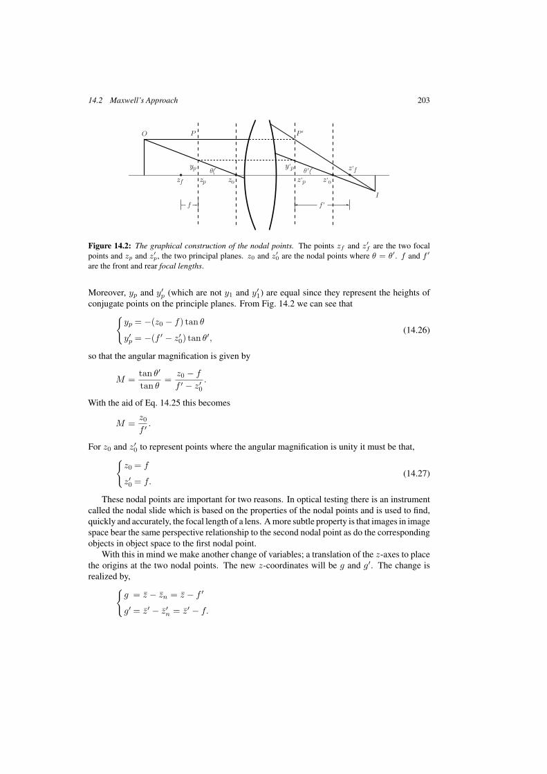
14.2 Maxwell’s Approach 203
Figure 14.2: The graphical construction of the nodal points. The points zf and z′f are the two focal
points and zp and z′p, the two principal planes. z0 and z′
0 are the nodal points where θ = θ′. f and f ′
are the front and rear focal lengths.
Moreover, yp and y′p (which are not y1 and y′
1) are equal since they represent the heights ofconjugate points on the principle planes. From Fig. 14.2 we can see that{
yp = −(z0 − f) tan θ
y′p = −(f ′ − z′
0) tan θ′,(14.26)
so that the angular magnification is given by
M =tan θ′
tan θ=
z0 − f
f ′ − z′0.
With the aid of Eq. 14.25 this becomes
M =z0
f ′ .
For z0 and z′0 to represent points where the angular magnification is unity it must be that,{
z0 = f
z′0 = f.
(14.27)
These nodal points are important for two reasons. In optical testing there is an instrumentcalled the nodal slide which is based on the properties of the nodal points and is used to find,quickly and accurately, the focal length of a lens. A more subtle property is that images in imagespace bear the same perspective relationship to the second nodal point as do the correspondingobjects in object space to the first nodal point.
With this in mind we make another change of variables; a translation of the z-axes to placethe origins at the two nodal points. The new z-coordinates will be g and g′. The change isrealized by,{
g = z − zn = z − f ′
g′ = z′ − z′n = z′ − f.
204 14 The Perfect Lenses of Gauss and Maxwell
Again using Newton’s formula, Eq. 14.20, we get
gg′ + gf + g′f ′ = 0,
from which comes,
f
g′ +f ′
g+ 1 = 0. (14.28)
This concludes the study of the ideal optical instrument. We have found the six cardinalpoints, the foci, the principal points and the nodal points, solely from considering the Maxwellmodel of an ideal instrument. The model is a static one; there is no mention of wavefronts,velocities or refractive indices.
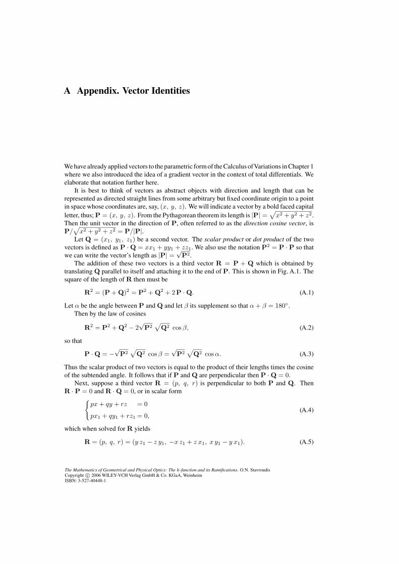
The Mathematics of Geometrical and Physical Optics: The k-function and its Ramifications. O.N. StavroudisCopyright c© 2006 WILEY-VCH Verlag GmbH & Co. KGaA, WeinheimISBN: 3-527-40448-1
A Appendix. Vector Identities
We have already applied vectors to the parametric form of the Calculus ofVariations in Chapter 1where we also introduced the idea of a gradient vector in the context of total differentials. Weelaborate that notation further here.
It is best to think of vectors as abstract objects with direction and length that can berepresented as directed straight lines from some arbitrary but fixed coordinate origin to a pointin space whose coordinates are, say, (x, y, z). We will indicate a vector by a bold faced capitalletter, thus; P = (x, y, z). From the Pythagorean theorem its length is |P| =
√x2 + y2 + z2.
Then the unit vector in the direction of P, often referred to as the direction cosine vector, isP/
√x2 + y2 + z2 = P/|P|.
Let Q = (x1, y1, z1) be a second vector. The scalar product or dot product of the twovectors is defined as P · Q = xx1 + yy1 + zz1. We also use the notation P2 = P · P so thatwe can write the vector’s length as |P| =
√P2.
The addition of these two vectors is a third vector R = P + Q which is obtained bytranslating Q parallel to itself and attaching it to the end of P. This is shown in Fig. A.1. Thesquare of the length of R then must be
R2 = (P + Q)2 = P2 + Q2 + 2P · Q. (A.1)
Let α be the angle between P and Q and let β its supplement so that α + β = 180◦.Then by the law of cosines
R2 = P2 + Q2 − 2√
P2√
Q2 cos β, (A.2)
so that
P · Q = −√
P2√
Q2 cos β =√
P2√
Q2 cos α. (A.3)
Thus the scalar product of two vectors is equal to the product of their lengths times the cosineof the subtended angle. It follows that if P and Q are perpendicular then P · Q = 0.
Next, suppose a third vector R = (p, q, r) is perpendicular to both P and Q. ThenR · P = 0 and R · Q = 0, or in scalar form{
px + qy + rz = 0
px1 + qy1 + rz1 = 0,(A.4)
which when solved for R yields
R = (p, q, r) = (y z1 − z y1, −x z1 + z x1, x y1 − y x1). (A.5)
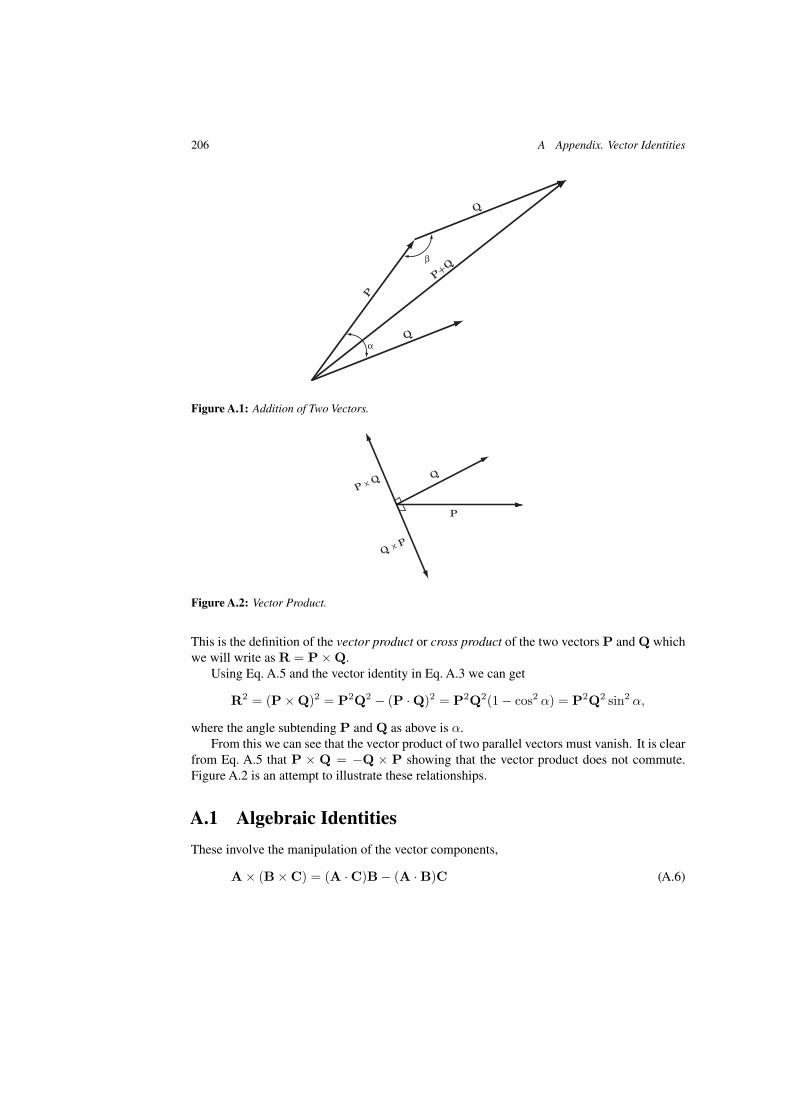
206 A Appendix. Vector Identities
Figure A.1: Addition of Two Vectors.
Figure A.2: Vector Product.
This is the definition of the vector product or cross product of the two vectors P and Q whichwe will write as R = P × Q.
Using Eq. A.5 and the vector identity in Eq. A.3 we can get
R2 = (P × Q)2 = P2Q2 − (P · Q)2 = P2Q2(1 − cos2 α) = P2Q2 sin2 α,
where the angle subtending P and Q as above is α.From this we can see that the vector product of two parallel vectors must vanish. It is clear
from Eq. A.5 that P × Q = −Q × P showing that the vector product does not commute.Figure A.2 is an attempt to illustrate these relationships.
A.1 Algebraic Identities
These involve the manipulation of the vector components,
A × (B × C) = (A · C)B − (A · B)C (A.6)

A.2 Identities Involving First Derivatives 207
(A × B) · (C × D) = (A · C)(B · D) − (A · D)(B · C) (A.7)
From Eq. A.6 we can get,
(A × B) × (C × D) = (A × B) · D C − (A × B) · C B (A.8)
and from Eq. A.7 comes,
(A × B)2 = A2 B2 − (A · B)2. (A.9)
A.2 Identities Involving First Derivatives
∇ · (γ E) = ∇γ · E + γ ∇ · E. (A.10)
∇ × (γ E) = ∇γ × E + γ ∇ × E. (A.11)
∇(E · F) = (E · ∇)F + (F · ∇)E + E × (∇ × F) + F × (∇ × E), (A.12)
∇ · (E × F) = F · (∇ × E) − E · (∇ × F), (A.13)
∇ × (E × F) = (F · ∇)E − (E · ∇)F + E(∇ · F) − F(∇ · E). (A.14)
Note the directional derivatives in Eqs. A.12 and A.14.
A.3 Identities Involving Second Derivatives
Here we introduce the Lagrangian operator,
∇2 = ∂2/∂x2 + ∂2/∂y2 + ∂2/∂z2. (A.15)
∇ · (∇Φ) = ∇2Φ, (A.16)
∇(∇ · A) = ∇2A − ∇ × (∇ × A), (A.17)
∇ × (∇Φ) = 0, (A.18)
∇ · (∇ × A) = 0. (A.19)
From Eq. A.17, if A2 = constant then,
(A · ∇)A = −A × (∇ × A). (A.20)
208 A Appendix. Vector Identities
A.4 Gradient
In Cartesian terms the gradient of a function f(x, y, z) is defined as ∇f= (∂f/∂x, ∂f/∂y, ∂f/∂z). To switch to the system of generalized coordinates we assumethat each of the arguments of f is a component of W and therefore a function of u, v and w.We take the derivatives of f with respect to these generalized coordinates and use the chainrule to get
∂f
∂v=
∂f
∂xxv +
∂f
∂yyv +
∂f
∂zzv
∂f
∂w=
∂f
∂xxw +
∂f
∂yyw +
∂f
∂zzw
∂f
∂s=
∂f
∂xxs +
∂f
∂yys +
∂f
∂zzs
or in matrix form
xv yv zv
xw yw zw
xs ys zs
fx
fy
fz
=
fv
fw
fs
.
The determinant of coefficients is∣∣∣∣∣∣∣∣xv yv zv
xw yw zw
xs ys zs
∣∣∣∣∣∣∣∣= xs(yvzw − ywzv) − ys(xvzw − xwzv) + zs(xvyw − yvzw)
= Ws · (Wv × Ww) = D,
where D is defined in Eqs. 4.8 and 6.10.With Cramer’s rule we solve for fx, fy , and fz to get
Dfx =
∣∣∣∣∣∣∣∣fv yv zv
fw yw zw
fs ys zs
∣∣∣∣∣∣∣∣= fv
∣∣∣∣∣yw ys
zs zw
∣∣∣∣∣ − fw
∣∣∣∣∣yv ys
zs zv
∣∣∣∣∣ + fs
∣∣∣∣∣yv yw
zw zv
∣∣∣∣∣
Dfy =
∣∣∣∣∣∣∣∣xv fv zv
zs xw fw
xs fs zs
∣∣∣∣∣∣∣∣= −fv
∣∣∣∣∣xw xs
zs zw
∣∣∣∣∣ + fw
∣∣∣∣∣xv xs
zs zv
∣∣∣∣∣ − fs
∣∣∣∣∣xv xw
zw zv
∣∣∣∣∣
Dfz =
∣∣∣∣∣∣∣∣xv yv fv
xw yw fw
xs ys fs
∣∣∣∣∣∣∣∣= fv
∣∣∣∣∣xw xs
ys yw
∣∣∣∣∣ − fw
∣∣∣∣∣xv xs
ys yv
∣∣∣∣∣ + fs
∣∣∣∣∣xv xw
yw yv
∣∣∣∣∣ .
A.5 Divergence 209
Then the gradient of f can be written as
D∇f = D(fx, fy, fz)
=
(fv
∣∣∣∣∣yw ys
zs zw
∣∣∣∣∣ − fw
∣∣∣∣∣yv ys
zs zv
∣∣∣∣∣ + fs
∣∣∣∣∣yv yw
zw zv
∣∣∣∣∣ ,
−fv
∣∣∣∣∣xw xs
zs zw
∣∣∣∣∣ + fw
∣∣∣∣∣xv xs
zs zv
∣∣∣∣∣ − fs
∣∣∣∣∣xv xw
zw zv
∣∣∣∣∣ ,
fv
∣∣∣∣∣xw xs
ys yw
∣∣∣∣∣ − fw
∣∣∣∣∣xv xs
ys yv
∣∣∣∣∣ + fs
∣∣∣∣∣xv xw
yw yv
∣∣∣∣∣)
= fv
(∣∣∣∣∣yw ys
zs zw
∣∣∣∣∣ ,−∣∣∣∣∣xw xs
zs zw
∣∣∣∣∣ ,
∣∣∣∣∣xw xs
ys yw
∣∣∣∣∣)
−fw
(∣∣∣∣∣yv ys
zs zv
∣∣∣∣∣ ,−∣∣∣∣∣xv xs
zs zv
∣∣∣∣∣ ,
∣∣∣∣∣xv xs
ys yv
∣∣∣∣∣)
+fs
(∣∣∣∣∣yv yw
zw zv
∣∣∣∣∣ ,−∣∣∣∣∣xv xw
zw zv
∣∣∣∣∣ ,
∣∣∣∣∣xv xw
yw yv
∣∣∣∣∣)
= (Wv × Ws)fv − (Wv × Ws)fw + (Wv × Ww)fs.
It follows from this that
∇f =1D
[(Wv × Ws)fv − (Wv × Ws)fw
]+ Wsfs. (A.21)
A.5 Divergence
Let V = (a, b, c). Then following the above
Dax =
∣∣∣∣∣∣∣∣av yv zv
aw yw zw
as ys zs
∣∣∣∣∣∣∣∣, Dbx =
∣∣∣∣∣∣∣∣bv yv zv
bw yw zw
bs ys zs
∣∣∣∣∣∣∣∣, Dcx =
∣∣∣∣∣∣∣∣cv yv zv
cw yw zw
cs ys zs
∣∣∣∣∣∣∣∣
Day =
∣∣∣∣∣∣∣∣xv av zv
xw aw zw
xs as zs
∣∣∣∣∣∣∣∣, Dby =
∣∣∣∣∣∣∣∣∣
xv bv zv
xw bw zw
xs bs zs
∣∣∣∣∣∣∣∣∣, Dcy =
∣∣∣∣∣∣∣∣xv cv zv
xw cw zw
xs cs zs
∣∣∣∣∣∣∣∣
Daz =
∣∣∣∣∣∣∣∣∣
xv yv av
xw yw aw
xs ys as
∣∣∣∣∣∣∣∣∣, Dbz =
∣∣∣∣∣∣∣∣xv yv bv
xw yw bw
xs ys bs
∣∣∣∣∣∣∣∣, Dcz =
∣∣∣∣∣∣∣∣xv yv cv
xw yw cw
xs ys cs
∣∣∣∣∣∣∣∣.
210 A Appendix. Vector Identities
Then
D ∇ · V = D(ax + by + cv)
=
∣∣∣∣∣∣∣∣av yv zv
aw yw zw
as ys zs
∣∣∣∣∣∣∣∣+
∣∣∣∣∣∣∣∣xv bv zv
xw bw zw
xs bs zs
∣∣∣∣∣∣∣∣+
∣∣∣∣∣∣∣∣xv yv cv
xw yw cw
xs ys cs
∣∣∣∣∣∣∣∣=
∣∣∣∣∣∣∣∣av bv cv
xw yw zw
xs ys zs
∣∣∣∣∣∣∣∣+
∣∣∣∣∣∣∣∣xv yv zv
aw bw cw
xs ys zs
∣∣∣∣∣∣∣∣+
∣∣∣∣∣∣∣∣xv yv zv
xw yw zw
as bs cs
∣∣∣∣∣∣∣∣= Vv · (Ww × Ws) − Vw · (Wv × Ws) + Vs · (Wv × Ww) .
It follows that the divergence of V is given by
∇ · V =1D
[Vv · (Ww × Ws) − Vw · (Wv × Ws)
]+ Ws · Vs. (A.22)
A.6 Curl
The curl of the vector V is defined as follows:
∇ × V = (cv − bz, −cx + az, bx − ay).
D (∇ × V) =
∣∣∣∣∣∣∣∣xv cv zv
xw cw zw
xs cs zs
∣∣∣∣∣∣∣∣−
∣∣∣∣∣∣∣xv yv bv
xw yw bw
xs ys zs
∣∣∣∣∣∣∣
,−
∣∣∣∣∣∣∣cv yv zv
cw yw zw
cs ys zs
∣∣∣∣∣∣∣ +
∣∣∣∣∣∣∣xv yv av
xw yw aw
xs ys as
∣∣∣∣∣∣∣
,
∣∣∣∣∣∣∣bv yv zv
bw yw zw
bs ys zs
∣∣∣∣∣∣∣ −
∣∣∣∣∣∣∣xv av zv
xw aw zw
xs as zs
∣∣∣∣∣∣∣ .
A.6 Curl 211
This reduces to
D (∇ × V)
=(bv(xsyw − xwys) + cv(xszw − xwzs),
−cv(ywzs − yszw) + av(xwys − xsyw),
bv(ywzs − yszw) + av(xwzs − xszw))
+(cw(xvzs − xszv) + bw(xvys − xsyv),
cw(yvzs − yszv) − aw(xvys − xsyv),
−bw(yvzs − yszv) − aw(xvzs − xszv))
+(
− cs(xvzw − xwzv) − bs(xvyw − xwyv),
−cs(yvzw − ywzv) + as(xvyw − xwyv),
bs(yvzw − ywzv) + as(xvzw − xwzv))
=(
− (avxs + bvys + cvzs)xw + (avxw + bvyw + cvzw)xs,
−(avxs + bvys + cvzs)yw + (avxw + bvyw + cvzw)ys,
−(avxs + bvys + cvzs)zw + (avxw + bvyw + cvzw)zs
)+
((awxs + bwys + cwzs)xv − (awxv + bwyv + cwzv)xs,
(awxs + bwys + cwzs)yv − (awxv + bwyv + cwzv)ys,
(awxs + bwys + cwzs)zv − (awxv + bwyv + cwzv)zs
)+
(− (asxw + bsyw + cszw)xv + (asxv + bsyv + cszv)xw,
−(asxw + bsyw + cszw)yv + (asxv + bsyv + cszv)yw,
−(asxw + bsyw + cszw)zv + (asxv + bsyv + cszv)zw
).
Now switching form a scalar to a vector notation, we get
D (∇ × V) =(
− (Vv · Ws)Ww + (Vv · Ww)Ws
)+
((Vw · Ws)Wv − (Vw · Wv)Ws
)+
(− (Vs · Ww)Wv + (Vs · Wv)Ww
)= (Ww × Ws) × Vv − (Wv × Ws) × Vw + (Wv × Ww) × Vs.
The final result for the curl of V is then
∇ × V =1D
[(Ww × Ws) × Vv − (Wv × Ws) × Vw
]+ Ws × Vs. (A.23)

212 A Appendix. Vector Identities
A.7 Lagrangian
The assertion is that the Lagrangian of the scalar functionQ(v, w, s) is given by
∇2Q = ∇ · (∇Q)
=1D
{Ww · ∂
∂v
(QvWw − QvWv
D
)
−Wv · ∂
∂w
(QvWw − QvWv
D
)+ DsQs
}+ Qss.
(A.24)
To show this, note that
QvWw − QvWv = (∇Q · Wv)Ww − (∇Q · Ww)Wv
= −∇Q × (Wv × Ww) = D(Ws × ∇Q).(A.25)
Inserting this into the right member of Eq. A.24 yields,
1D
{Ww · ∂
∂v(Ws × ∇Q) − Wv · ∂
∂w(Ws × ∇Q) + DsQs
}+ Qss
=1D
{Ww · [(Wvs × ∇Q) + Ws × (∇Q)v]
−Wv · [(Wws × ∇Q) + Ws × (∇Q)w] + DsQs
}+ Qss
=1D
{− (Wv × Ww)s · ∇Q
+[(Ww × Ws) · (∇Q)v − (Wv × Ws) · (∇Q)w] + DsQs
}+ Qss
=1D
{− Ds(Ws · ∇Q) + D[∇ · (∇Q)− (∇Q)sWs] + DsQs
}+ Qss
= ∇ · (∇Q) = ∇2Q,
which was to be shown.
A.8 Directional Derivative
Let A = (a, b, c) and let P be any vector. Then
(P · ∇)A =((P · ∇a), (P · ∇b), (P · ∇c)
)=
1D
(P · (Ww × Ws)av − P · (Wv × Ws)aw + D(P · Ws)as,
P · (Ww × Ws)bv − P · (Wv × Ws)bw + D(P · Ws)bs,
P · (Ww × Ws)cv − P · (Wv × Ws)cw + D(P · Ws)cs
)=
1D
[P · (Ww × Ws)Av − P · (Wv × Ws)Aw + D(P · Ws)As
].

A.9 Operations on W and its Derivatives 213
From this we get
(P · ∇)A =1D
[(Ws × P) · Ww Av − (Ws × P) · Wv Aw
]+ (Ws · P) As.
(A.26)
A.9 Operations on W and its Derivatives
Now we are able to apply these results to the vector W and its derivatives. Here we useEq. A.22 to get
∇ · W =1D
[(Ww × Ws) · Wv − (Wv × Ws) · Ww
]+ W2
s
=1D
[2(Wv × Ww) · Ws
]+ 1
= 3.
(A.27)
The divergences of the derivatives are done in the same way,
∇ · Wv =1D
[(Ww × Ws) · Wvv − (Wv × Ws) · Wvw
]+ Ws · Wvs
=1D
[(Wvv × Ww) · Ws + (Wv × Www) · Ws
]=
1D
[(Wv × Ww)v · Ws
]=
Dv
D.
(A.28)
Here we have made use of the fact that Wv ·Ws = 0 and that Ws = (1/D)(Wv ×Ww). Inexactly the same way we can get
∇ · Ww =Dw
D. (A.29)
Now for the curls. First we will need the first and second fundamental quantities definedas
E = W2v F = Wv · Ww G = W2
w
L = Ws · Wvv M = Ws · Wvw N = Ws · Www.(A.30)
The derivatives of the first fundamental quantities are as follows:
Es = 2Wv · Wvs, Fs = Wvs · Ww + Wv · Wws, Gs = 2Ww · Wws
Ev = 2Wv · Wvv, Fv = Wvv · Ww + Wv · Wws, Gv = 2Ww · Wwv
Ew = 2Wv · Wvw, Fw = Wvw · Ww + Wv · Wws, Gw = 2Ww · Www,
(A.31)

214 A Appendix. Vector Identities
from which we can see that
L = −Es/2 M = −Fs/2 N = −Gs/2. (A.32)
In addition note that, since Ws · Wv and Ws · Ww both equal zero,
Wvs · Ww = Wws · Wv = −Ws · Wvw . (A.33)
Now turn to the calculations of the curls using Eq. A.23. First we show that the curl of W iszero.
∇ × W =1D
[(Ww × Ws) × Wv − (Wv × Ws) × Ww
]= − 1
D
[(Wv · Ws)Ww − (Wv · Ww)Ws
−(Ww · Ws)Wv + (Ww · Wv)Ws
]= 0,
(A.34)
from Eq. A.33. In exactly the same way we can show that ∇ × Ws = 0. Next we do Wv ,which is
∇ × Wv =1D
[(Ww × Ws) × Wvv − (Wv × Ws) × Www
]+ Ws × Wvs
= − 1D
[(Wvv · Ws)Ww − (Wvv · Ww)Ws
−(Wvw · Ws)Wv + (Wvw · Wv)Ws
]+ Ws × Wvs
=1
2D
[EsWw − FsWv + 2(Ew − Fv)Ws
]+ Ws × Wvs.
(A.35)
The calculation of curl Ww proceeds in the same way and is
∇ × Ww =1
2D
[FsWw − GsWv + 2(Fw − Gv)Ws
]+ Ws × Wws. (A.36)
A.10 An Additional Lemma
We sometimes encounter expressions of the type
Ww · Vv − Wv · Vw. (A.37)
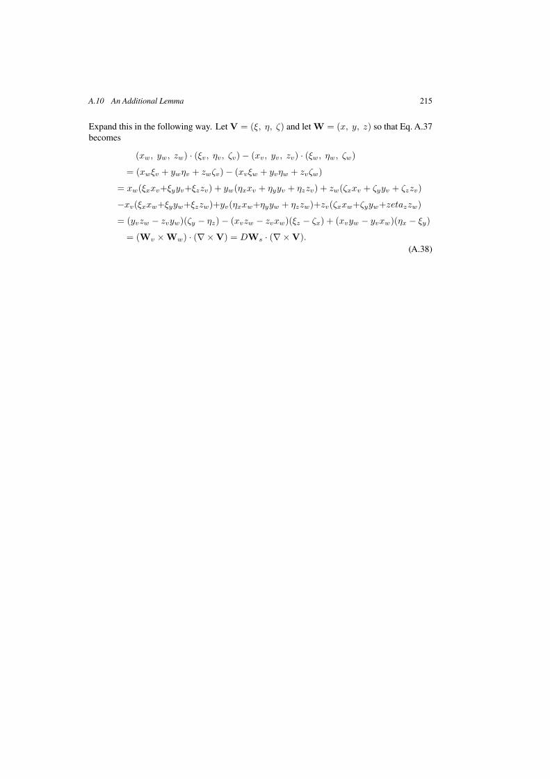
A.10 An Additional Lemma 215
Expand this in the following way. Let V = (ξ, η, ζ) and let W = (x, y, z) so that Eq. A.37becomes
(xw, yw, zw) · (ξv, ηv, ζv) − (xv, yv, zv) · (ξw, ηw, ζw)
= (xwξv + ywηv + zwζv) − (xvξw + yvηw + zvζw)
= xw(ξxxv+ξyyv+ξzzv) + yw(ηxxv + ηyyv + ηzzv) + zw(ζxxv + ζyyv + ζzzv)
−xv(ξxxw+ξyyw+ξzzw)+yv(ηxxw+ηyyw + ηzzw)+zv(ζxxw+ζyyw+zetazzw)
= (yvzw − zvyw)(ζy − ηz) − (xvzw − zvxw)(ξz − ζx) + (xvyw − yvxw)(ηx − ξy)
= (Wv × Ww) · (∇ × V) = DWs · (∇ × V).(A.38)
The Mathematics of Geometrical and Physical Optics: The k-function and its Ramifications. O.N. StavroudisCopyright c© 2006 WILEY-VCH Verlag GmbH & Co. KGaA, WeinheimISBN: 3-527-40448-1
B Bibliography
Altrichter and Schafer 1956: O. Altrichter and G. Schafer, “Herleitung der Gullstrand-schen Grundgleichungen fur Schiefe Strahlenbuschel aus den Hauptkrummungen derWellenflache”Optik(Stuttgart) 13, 241–253.
Avendano-Alejo and Stavroudis 2002: M. Avendano-Alejo and O.N. Stavroudis, “Huy-gens principle and rays in uniaxial anisotropic media. II. Crystal axis orientation arbitrary.” J.Opt. Soc. Am. A 19, 1674–1679.
Avendano-Alejo et al. 2004: M.Avendano-Alejo, J. Orozco-Arellanes and O.N. Stavroudis,“Spherical aberrations analysis of an uniaxial Cartesian oval.” SPIE 5622, 1164–1168.
Blaschke 1945: Wilhelm Blaschke, Vorlesungen uber Differential Geometrie. Dover Pub-lications, New York.
Bliss 1925: Gilbert A. Bliss, Calculus of Variations. The Mathematical Association ofAmerica, Carus Mathematical Monograph #19, Open Court Publishing Co, LaSalle, Indiana.
Bliss 1946: Gilbert A. Bliss, Lectures on the Calculus of Variations. The University ofChicago Press.
Bolza 1961: Oskar Bolza, Lectures on the Calculus of Variations. Dover Publications,New York. [1904: University of Chicago Press.]
Born and Wolf 1999: Max Born and Emil Wolf, Principles of Optics. 7th Edition. Cam-bridge University Press.
Buchdahl 1970: H. A. Buchdahl, An Introduction to Hamiltonian Optics. CambridgeUniversity Press.
Buchdahl 1972: H. A. Buchdahl, “Systems without Symmetries: Foundations of a Theoryof Lagrangian Aberration Coeficients.” J. Opt. Soc. Am. A 62 1314–1324.
Buchroeder 1970: R. A. Buchroeder,“ Tilted Component Telescopes. Part 1: Theory.”Appl. Opt. 9, 2169–2171.
Cagnet et al 1962: M. Cagnet, M. Francon and J. C. Thrier, The Atlas of Optical Phenom-ena. Prentice Hall, Englewood Cliffs, N. J.
Caratheodory 1989: C. Caratheodory, Calculus of Variations and Partial DifferentialEquations of the First Order. Tr. Robert B. Dean, Tr. Editor Julius J. Brandstatter. AMS
218 B Bibliography
Chelsea Publishing, American Mathematicial Society, Providence, RI. [Variationsrechnungund Partielle Differentialgleichnungen erster Ordnung. 1935: B. G. Teubner, Berlin.]
Cohen 1933: Abraham Cohen, An Elementary Treatise on Differential Equations. SecondEdition. D. C. Heath & Co.
Coddington 1829–1830: H. Coddington, A System of Optics in two volumes. Limkin andMarshal, London.
Courant and Robbins 1996: Richard Courant and Herbert Robbins, What is Mathematics?Revised by Ian Stewart, Oxford University Press, New York.
Clegg 1968: John C. Clegg, Calculus of Variations. John Wiley & Sons, New York.
Conway and Synge 1931: A. W. Conway and J. L. Synge, The Mathematical Papers ofSir William Rowan Hamilton. Vol. I. Geometrical Optics. Cambridge University Press.
Dickson 1914: Leonard Eugene Dickson, Elementary Theory of Equations. John Wiley &Sons, New York.
Dickson 1939: Leonard Eugene Dickson, New First Course in the Theory of Equations.John Wiley & Sons, New York.
Do Carmo 1976: Manfredo P. Do Carmo, Differential Geometry of Curves and Surfaces.Prentice-Hall, Englewood Cliffs, New Jersey.
Flores-Hernandez and Stavroudis 1996: R. Flores-Hernandez and O.N. Stavroudis,“Real time manipulations of the Delano diagram as a linear tool for optical system optimiza-tion”, Optik 4, 141–147.
Forsyth 1959: Andrew Russell Forsyth, Theory of Differential Equations. Six volumesbound as three. Dover Publications, New York. [A reprint of Cambridge University Press,1906.]
Forsyth 1996: Andrew Russell Forsyth, A Treatise on Differential Equations. Sixth Edi-tion. Dover Publications, Mineola, New York.
Garabedian 1998: P. R. Garabedian, Partial Differential Equations. AMS Chelsea Pub-lishing, Providence, Rhode Island.
Gelles 1974: R. Gelles, “Unobscured Aperture Stigmatic Telescopes.” Opt. Eng. 13,534–538.
Gelles 1975: R. Gelles, “Unobscured Aperture Two-Mirror Systems.” J. Opt. Soc. Am. A65, 1141–1143.
Goursat 1904: Edouard Goursat, A Course in Mathematical Analysis. Translated ed byEarle Raymond Heddrick. Ginn & Co. Boston.
Goursat 1945: Edouard Goursat, Differential Equations. Translated ed by Earle RaymondHeddrick and Otto Dunkel. Ginn & Co. Boston.
Gugenheimer 1977: Heinrich W. Gugenheimer, Differential Geometry. Dover Publica-tions, New York.
219
Gullstrand 1906: A. Gullstrand, “Die reelle optische Abbildung.” Sv. Vetensk. Handl.41, 1–119.
Herzberger 1935: Max Herzberger, “On the fundamental optical invariant, the opticaltetrality principle, and on the new development of Gauss optics based on this law.” J. Opt.Soc. Am. 25, 197–204
Herzberger 1936: Max Herzberger, “A new theory of optical image formation.” J. Opt.Soc. Am. 26, 295–304.
Herzberger 1937: Max Herzberger, “Optics in the large.” J. Opt. Soc. Am. 27, 202–206.
Herzberger 1939: Max Herzberger, “Normal systems with two caustic lines.” J. Opt.Soc. Am. 29, 392–394.
Herzberger 1940: Max Herzberger, “Normal systems with two caustic lines.” J. Opt.Soc. Am. 30, 307–308.
Herzberger 1943a: Max Herzberger, “Direct methods in geometrical optics.” Trans. Am.Math. Soc. 53, 218–229.
Herzberger 1943b: Max Herzberger, “A direct image error theory.” Q. Appl. Math. 1,69–77.
Herzberger 1946: Max Herzberger, “The Limitation of Optical Image Formation, Pointsand Diapoints.” Ann. N. Y. Acad. Sci. 48, 7–13.
Herzberger 1954a: Max Herzberger, “Some remarks on ray tracing.” J. Opt. Soc. Am.41, 805–807.
Herzberger 1954b: Max Herzberger, “Image errors and diapoint errors.” In Studiesin Mathematics and Mechanics presented to Richard von Mises by Friends, Colleagues andPupils. Academic Press, New York. pp. 30–35.
Herzberger 1958: Max Herzberger, Modern Geometrical Optics. John Wiley & Sons(Interscience), New York.
Ito 1993: Kiyosi Ito, Editor. Encyclopedic Dictionary of Mathematics. Second Edition.MIT Press, Cambridge MA and London.
Joos 1941: G. Joos, Theoretical Physics. Tr. I. M. Freeman, Blackie & Son, London.
Kline and Kay 1965: M. Kline and I. W. Kay, Electromagnetic Theory and GeometricalOptics. Interscience/John Wiley & Sons.
Kemmer 1977: N. Kemmer, Vector Analysis. A physicist’s guide to the mathematics offields in three dimensions. Cambridge University Press.
Kneisly 1964: J. A. Kneisly III, “Local curvatures of wavefronts in an optical system.” J.Opt. Soc. Am. 54, 229–235.
Korn and Korn 1968: G. A. Korn and T. M. Korn, Mathematical Handbook for Scientistsand Engineers. Second Edition. McGraw-Hill, New York.
220 B Bibliography
Korsch 1991: Dietrich Korsch, Reflective Optics. Academic Press, San Diego.
Kutter 1953: Anton Kutter, Der Schiefspiegler. Biberacher Verlagsdruckerei, Biberach ander RiS, Germany.
Kutter 1969: A. Kutter, Sky and Telescope 38 418 (1969). Cited in Buchroeder 1970.
Luneburg 1964: R. K. Luneburg, Mathematical Theory of Optics. University of CaliforniaPress, Berkeley. Reprint of notes given for a course at Brown University, 1944.
Malacara and Thompson 2001: Daniel Malacara and Brian J. Thompson, Handbook ofOptical Engineering. Marcel Dekker, Inc., New York.
Marion and Heald 1980: J. B. Marion and M. A. Heald, Classical ElectroMagneticRadiation. 2nd Ed. Academic Press, New York.
Maxwell 1952: James C. Maxwell, Scientific Papers. W. D. Niven, Editor. Dover Publi-cations, New York.
O’Connell 1998: James O’Connell, “Review of Maxwell on the Electromagnetic Field: AGuided Study.” Am. J. Phys. 66, 92–93.
Rektorys 1969: Karel Rektorys, Survay of Applicable Mathematics. The M. I. T. Press,Cambridge, Massachusetts.
Sabra 1967: A. I. Sabra, Theories of Light. From Descartes to Newton. Oldbourne,London.
Sands 1972: P. J. Sands, “Aberration Coeficients of Plane Symmetric Systems.” J. Opt.Soc. Am. A 62, 1211–1220.
Sands 1973a: P. J. Sands, “Aberration Coeficients of Double-Planeª Symmetric Systems.”J. Opt. Soc. Am. A 63, 425–430.
Sands 1973b: P. J. Sands, “Thin Double-Plane Symmetric Systems.” J. Opt. Soc. Am. A63, 431–434.
Smith 1959: David Eugene Smith, A Source Book in Mathematics. Dover Publications,New York. [1929: McGraw-Hill Book Co.]
Stavroudis and Sutton 1965: O. N. Stavroudis and L. E. Sutton, Spot Diagrams for thePrediction of Lens Performance from Design Data. NBS Monograph No. 93 U. S. GovernmentPrinting Office. Washington, DC.
Stavroudis 1967: O. N. Stavroudis, “Resolving power predictions from lens design data.”Appl. Opt. 6 129–135.
Stavroudis 1972a: O. N. Stavroudis, The Optics of Rays, Wavefronts and Caustics. Aca-demic Press, New York.
Stavroudis 1972b: O. N. Stavroudis, “Some consequences of Herzberger’s fundamentaloptical invarient.” J. Opt. Soc. Am. 62, 59–63.
Stavroudis 1976: O. N. Stavroudis, “A simpler derivation of the formulas for generalizedray tracing.” J. Opt. Soc. Am. 66, 1330–1333.

221
Stavroudis and Fronczek 1976: O. N. Stavroudis and R. C. Fronczek, “Caustic surfacesand the structure of the geometric image.” J. Opt. Soc. Am. 66, 795–800.
Stavroudis et al. 1978: O. N. Stavroudis, R. Fronczek and R.-S. Chang, “The geometryof the half symmetric image.” J. Opt. Soc. Am. 68, 739–742.
Stavroudis and Fronczek 1978: O. N. Stavroudis and R. Fronczek, “Generalized raytracing and the caustic surface.” Optics and Laser Technology 10, 185–191.
Stavroudis andAmes 1992: O. N. Stavroudis andA. J.Ames, “Confocal Prolate Spheroidsin an Off-Axis System.” J. Opt. Soc. Am. A 9, 2083–2088 (1992).
Stavroudis 1995a: O. N. Stavroudis, “The k-function in geometrical optics and its re-lationship to the archetypical wave front and the caustic surface.” J. Opt. Soc. Am. A 12,1010–1016.
Stavroudis 1995b: O. N. Stavroudis, “Refraction of the k-function at spherical surfaces.”J. Opt. Soc. Am. A 12, 1805–1811.
Stavroudis 1996: O. N. Stavroudis,“The caustic as an expression of the image errors of alens.” In: OSA Proceedings of the International Optical Design Conference, 1994, Vol. 22,Ed. G. W. Forbes, pp. 87–91.
Stavroudis and Flores-Hernandez 1998: O. N. Stavroudis and R. Flores-Hernandez,“Structure of the modern schiefspiegler. I. Pseudo axis, magnification, and distortion”, J. Opt.Soc. Am. A 15, 437–442.
Stavroudis 2001: “Basic Ray Optics.” In: Handbook of Optical Engineering DanielMalacara and Brian J. Thompson, Eds. Marcel Decker, New York and Basel. pp. 1–38.
Stoker 1969: J. J. Stoker, Differential Geometry. Wiley–Interscience, New York.
Stone and Forbes 1992a: B. D. Stone and G. W. Forbes, “Foundations of First-OrderLayout for Asymmetric Systems: An Application of Hamilton’s Methods.” J. Opt. Soc. Am.A 9, 96–109.
Stone and Forbes 1992b: B. D. Stone and G. W. Forbes, “First Order Layout of Asym-metric Systems Composed of Three Spherical Mirrors.” J. Opt. Soc. Am. A 9, 110–120.
Stone and Forbes 1992c: B. D. Stone and G. W. Forbes, “Characterization of First-OrderOptical Properties for Asymmetric Systems.” J. Opt. Soc. Am. A 9, 478–489.
Stone and Forbes 1992d: B. D. Stone and G. W. Forbes,“Forms of the CharacteristicFunction for Asymmetric Systems that Form Sharp Images to the First Order.” J. Opt. Soc.Am. A 9, 820–831.
Stone and Forbes 1992e: B. D. Stone and G. W. Forbes, “First-Order Layout of Asym-metric Systems: Sharp Imagery of a Single Plane Object.” J. Opt. Soc. Am. A 9, 832–843.
Struik 1961: Dirk J. Struik, Lectures on Classical Differential Geometry. Second Edition.Addison-Wesley, Reading, MA.
222 B Bibliography
Todhunter 1961: I. Todhunter, A History of the Calculus of Variations. Chelsia PublishingCo., New York. [A reprint of A History of the Progress of the Calculus of Variations duringthe Nineteenth Century. 1861: Cambridge]
Troutman 1983: John L. Troutman, Variational Calculus with Elementary Convexity.Springer-Verlag, New York.
Washer 1965: F. E. Washer, Phot.Eng. 52, 213 (1966).
Welford 1974: W. T. Wellford, Aberrations of the Symmetrical Optical System. AcademicPress, London.
Woodhouse 1964: Robert Woodhouse, A History of the Calculus of Variations in theEighteenth Century. Chelsea, Bronx, NY. [A reprint of A Treatise on Isoperimetrial Problemsand the Calculus of Variations. 1810.]
Young E. 1993: Eutiquio C. Young, Vector and Tensor Analysis. Second Edition. MarcelDekker, New York.
Young L. 1969: L. C. Young, Lectures on the Calculus of Variations and Optimal ControlTheory. W. B. Saunders Company, Philadelphia.
The Mathematics of Geometrical and Physical Optics: The k-function and its Ramifications. O.N. StavroudisCopyright c© 2006 WILEY-VCH Verlag GmbH & Co. KGaA, WeinheimISBN: 3-527-40448-1
Index
aberration theory 29, 121–129, 177chromatic 122hierarchical system 127, 129
anisotropic medium 12, 13antenna theory 147aplanatic points of a sphere 179, 185arc length parameter 10, 16, 19, 21, 25, 38,
45, 47, 54archetypical wavefront 131astigmatism 121asymptotic curves 60, 61, 94–96
back focal distance 11Bernoulli, Jacob 3Bernoulli, Jean 3bilinear concomitant 68, 71–73binormal vector 17, 19, 22, 25, 26, 54, 188brachistochrone 3Buchroeder, Richard 165
Calculus of Variations 3–7, 10, 11, 29, 51,67, 205
fixed end points 29parametric form 7, 8, 15vector notation 9, 10
canonical variables 41cardinal points 197Cartesian oval 179–183caustic surface 89, 90, 96, 98, 113, 121, 127,
128, 131, 147characteristics, method of 68–70chief rays 116, 166, 172, 173, 176, 177circle, osculating 17coma 121common focus 166, 168, 169, 171conic constant 22conic section 22–25, 61
of revolution 61, 119, 165, 167, 182conjugate points 41, 179, 203corpuscules 3cosine, direction 85, 97, 102, 114, 122, 148,
167, 169, 172, 205cross product (see vector product)curl 32, 37, 147, 149, 153, 154, 158, 190–
193, 210, 211, 213, 214curvature, line of 46, 60, 105, 189
curvature, principal 50, 51, 60, 63, 85, 89,90, 93, 94, 97, 99, 100, 105, 106,112–114, 116, 118
cycloid 3
deformation error 127derivative, directional 20, 21, 32, 107, 150,
151, 158, 188, 207, 212, 213derivative, total 7, 9, 31, 64Descartes, Rene 179dialectic method of Sylvester 142diapoint 102, 122, 127differential equation, total 19, 32, 34, 35–37,
42, 60, 68–71, 74, 77, 128exact 21
differential geometry 45, 148of curves 46of surfaces 45–65, 85
differential operator 20, 32dipole oscillator 147direction vector 51, 88, 115direction, isotropic 94direction, principal 50–52, 55, 57, 59, 60, 63,
85, 88, 93, 94, 97, 99, 100, 105, 106,112–114, 116
distal focus of ellipse 23distortion 101, 121, 166, 175–177divergence 147, 149, 150, 154, 156, 158,
190–192, 209, 210, 213
eccentricity 22, 23, 61, 168, 177, 182, 183eikonal 43, 67, 80, 90, 121eikonal equation 29, 43, 67, 77–81, 85, 91,
121, 126, 131, 147–149, 162electric field vector 147, 153, 192eliminant 142ellipse 22, 23, 25, 61, 118, 168, 182, 183entrance pupil 101, 166envelope 89equation, differential 15, 24, 26, 27, 29, 35–
37, 41–43, 61, 67–77, 96, 128, 143,160, 162, 179
equation, homogeneous 68, 70equation, inhomogeneous 68, 70equivalence relation 146Euler, Leonard 3

224 Index
Euler equations 7–10, 12, 15, 26, 29, 31, 33–35, 37, 41, 51–53
exactness, condition for 36, 37, 43, 72exit pupil 113, 162, 166extremal arc 3, 4, 7extremum 3–5, 40, 49–51
Fermat, Pierre de 3, 15, 16Fermat’s principle 3, 4, 15, 40, 67, 187field curvature 121field errors 121field of extremals 7, 29–32, 35, 41first fundamental form 47, 61, 87first fundamental quantities 47, 56, 58, 60,
62, 86, 87, 92, 100, 105, 213focal length 197, 203
front 201, 203rear 201, 203
focal plot (see spot diagram)focus, distal 23, 25, 61, 113, 117, 118, 165–
170, 172, 181–184focus, proximal 23, 25, 61, 114, 116–118,
165–170, 181–184formulas, reflection 171, 172fractional-linear transformation 198Frenet-Serret equations 18, 20, 22, 47, 54,
106, 107, 188, 189function of position 10, 12, 147, 187function, arbitrary 8, 67, 69, 70, 73–76, 80,
81, 85, 143, 158, 162function, homogeneous 8, 13, 70
Gauss, Carl Friedrich 197Gauss’ theorem 49, 50, 94Gaussian curvature 90generalized coordinates 147, 149, 208generating ellipse 167geodesic 51, 53, 54, 106, 108, 189geodesic curve 51, 53, 54, 59, 93, 94, 107gradient 20, 26, 32, 34, 37, 65, 100, 134, 147,
153, 205, 208, 209
half-symmetric image 127–129Hamilton’s characteristic function 43Hamilton-Jacobi equation 36, 41–43Hamiltonian 3, 41, 42helix, cylindrical 21, 22, 37–39
pitch 21Hertz 147
Herzberger, Max 122, 125, 127, 129, 182Herzberger’s diapoint 97, 102, 122, 131Hilbert, David 29Hilbert Integral 29–43
parametric case 33homogeneous optical medium 4hyperboloid of two sheets 61, 99, 177, 179,
183
ideal optical instrument 199, 202, 204image space 122, 124–126, 133, 170, 172,
173, 176, 185, 197–200, 202, 203index of refraction (see refractive index)inhomogeneous optical medium 4, 10, 187initial and terminal points 3integrability, condition for 36, 37integral, complete 67, 68, 73, 74, 76–81, 90,
128, 131integral, line 31, 34integral, variational 4, 5, 7, 9, 12, 29, 30, 33,
34, 38, 52integrating factor 36, 37, 145isotropic optical medium 4
Jacobian 56, 71, 72, 75, 76, 79, 125–127
k-function 80, 81, 85, 90, 91, 96, 121, 122,126, 127, 129, 131, 132, 136, 137,147, 158, 162 187
Kay, I.W. 191Kepler, Johannes 179Kline, M. 191Kutter, Anton 165, 167, 177
Lagrange invariant 104Lagrange, method of 67, 68, 143Lagrangian operator 207
of a scalar function 212latus rectum 23, 61, 168, 182, 183lens equation 125Luneburg 78, 91, 131
magnetic field vector 147, 153, 192magnification 166, 176, 177, 197, 201
angular 166, 177, 202, 203marginal rays 121maximum (see also extremum) 3, 4, 49, 51Maxwell, James C. 11, 179, 197, 198Maxwell equations 147–153, 158, 187

Index 225
for inhomogeneous media 187Maxwell’s fish eye 10, 11, 26, 27, 197mean value theorem 16media, homogeneous 45, 67, 77, 85, 97, 108,
187, 190media, inhomogeneous 10, 97, 122, 187meridional plane 97, 102, 104, 122, 127, 128method of Lagrange and Charpit 68, 72, 73,
77, 128extended by Jacobi 67, 72
Meusnier’s Theorem 47–49, 53
nodal point 197, 202–204nodal slide 197, 203normal congruence 29, 34normal vector 17–19, 22, 24, 25, 40, 46–50,
52, 62, 64, 87, 99, 100, 106, 114,122, 124, 136, 148, 167, 170, 179,188, 189
off-axis system 99, 165, 167optical path length 4, 40, 67, 68, 77, 78, 80,
81, 121, 123, 124, 127, 131, 133,179, 180
optical testing 203orthogonal surface 29, 35, 43orthonormal vector 17orthotomic system 29, 34, 131, 147osculating circle 17osculating plane 17ovaloid 181, 186
parameter transformation 46, 55, 56, 85, 92–94, 104
parametric curve 45–47, 54, 55, 57, 58, 60,62, 104, 189
paraxial approximation 103, 104paraxial chief ray 104paraxial marginal ray 104paraxial optics 197paraxial ray tracing 103perfect image 4, 121, 184–186perfect lens, Gauss and Maxwell 197plane of constant phase or wavefront 43plane of incidence 40, 101, 105, 112, 115,
181plane, rectifying 17point of incidence 40, 98–101, 106, 113, 114,
116, 118, 167, 168, 170, 171, 180
points of incidence 99, 122polar axis 22, 23, 61, 63, 167polynomial 51, 88, 89, 94, 99, 142, 144, 145
discriminant 95, 127quadratic 50, 88, 93–95, 127, 142, 144,
182quartic 179, 181sextic 143
potential function 147scalar 147vector 147
primary aberrations 121principal paraxial ray 121principal planes 201–203principal points 197, 201, 202prolate spheroid 61, 99, 113, 114, 116, 168,
177, 179, 182, 183proximal focus of the ellipse 23pseudo axis 166, 169, 170, 172–177pseudo Maxwell equation 187, 189
radius of curvature 17, 25, 49, 118ray equation 10, 11, 16, 25, 26, 34ray tracing 97, 101, 102, 112, 121–123, 167,
197generalized 97, 99, 100, 104, 105, 109,
112, 113, 117, 119graphic 185, 197refraction 112transfer 112
reduced ray direction cosines 40, 125, 129,131, 141
reduced ray vector 101, 132refracted ray 101, 105, 133refracting plane 131refraction equation 100, 101, 103, 106, 123,
179refractive index 3, 4, 10–12, 37, 39, 77, 97,
98, 114, 132, 133, 148, 197
saddle point 95scalar product 9, 13, 26, 51, 54, 101, 124,
152, 153, 155, 157, 205schiefspiegler 165
modern 99, 165–168, 177second fundamental form 48, 60second fundamental quantities 48, 49, 53, 57,
60, 62, 87, 92–94, 100, 105, 213Seidel aberrations 104, 121, 165

226 Index
sharp image 127, 129skew rays 102, 104, 122skewness invariant 102, 104Snell’s law 3, 29, 39, 40, 101, 105
scalar form 40, 101, 103vector form 40, 100, 109, 110, 136
sphere 46spherical coordinates 147spherical refracting surface 131–133spherical wavefront 25, 90–92, 116, 129,
131, 132, 140, 141, 147, 158–162spheroid, axes 115spot diagram 101, 102, 119standard form of conic section 22star image test 102surface area, element of 87surface of constant phase 67, 77surface, geodesic 51symmetric image 127, 129
tack point 17tangent, Euclidean definition 15time of transit 3, 4
torsion 18, 19, 21, 22, 25–27, 59, 106, 108,190
trajectory 3, 4transfer equation 104, 113, 123transversal 31, 32, 34, 35, 41transversal surface 35, 42, 43trihedron, vector 16–18, 20, 188, 192
umbilical point 94, 118
variational calculus (see Calculusof Variations)vector product 26, 40, 46, 62, 64, 113, 149,
151, 156, 191, 206velocity of light 4, 149vertex, ellipse 23
wavefronttrain 45, 68, 80, 81, 85, 90, 91, 96, 104,
126, 127, 131–137, 140, 146–148,158, 162
Weingarten equations 53–55, 105
0000
0000