Geometrical Calibration of a 2.5D Periapical Radiography ...

Appl. Sci. 2020, 10, 906; doi:10.3390/app10030906 www.mdpi.com/journal/applsci

Article

Geometrical Calibration of a 2.5D Periapical

Radiography System

Che‐Wei Liao 1, Ming‐Tzu Tsai 2, Heng‐Li Huang 3,4, Lih‐Jyh Fuh 3,5, Yen‐Lin Liu 6, Zhi‐Teng Su 3

and Jui‐Ting Hsu 3,4,*

1 Graduate Institute of Biomedical Sciences, China Medical University, Taichung 404, Taiwan;

[email protected] 2 Department of Biomedical Engineering, Hungkuang University, Taichung 433, Taiwan;

[email protected] 3 School of Dentistry, College of Dentistry, China Medical University, Taichung 404, Taiwan;

[email protected] (H.H.), [email protected] (L.F.), [email protected] (Z.S.) 4 Department of Bioinformatics and Medical Engineering, Asia University. Taichung 413, Taiwan 5 Department of Dentistry, China Medical University and Hospital, Taichung 404, Taiwan 6 Department of Biomedical Imaging and Radiological Science, China Medical University,

Taichung 404, Taiwan

* Correspondence: [email protected]; Tel.: +886‐4‐2205‐3366 ext. 2308

Received: 30 December 2019; Accepted: 27 January 2020; Published: 30 January 2020

Abstract: The objective of this study was to develop a geometrical calibration method applicable to

the 2.5D prototype Periapical Radiography System and estimate component position errors. A two‐

steel‐ball phantom with a precisely known position was placed in front of a digital X‐ray sensor for

two‐stage calibration. In the first stage, the following three parameters were estimated: (1) r, the

distance between the focal spot and the rotation axis of the X‐ray tube; (2) ψ, the included angle

between the straight line formed by the X‐ray tube’s focal spot and rotation axis and the straight

line of the orthogonal sensor; and (3) L4, the distance between the rotation axis and the plane where

the two steel balls were positioned. In the second stage, the steel balls’ positions were determined

to calculate the positions of the X‐ray tube on the x, y, and z axes. Computer simulation was used

to verify the accuracy of the calibration method. The results indicate that for the calibration

approach proposed in this study, the differences between the estimated errors and setting errors

were smaller than 0.15% in the first and second stages, which is highly accurate, verifying its

applicability to accurate calibration of the 2.5D Periapical Radiography System.

Keywords: geometric calibration; periapical radiography; computed tomosynthesis; quasi‐3D

imaging; 2.5D

1. Introduction

The application of X‐ray radiography in clinical dentistry is prevalent. Currently, dental

radiographic images can be divided into 2D and 3D radiographic images, and 2D radiographs can be

further divided into intraoral and extraoral. Equipment for capturing intraoral radiographs includes

periapical, bitewing, and occlusal films, whereas that for extraoral radiographs includes panoramic

and cephalometric films. The most substantial problem related to 2D radiographs is the superposition

of tissue images, which leads to dentists being unable to accurately determine the solid forms of teeth

or bone structures [1,2]. The commonest form of 3D radiography is cone beam computed tomography

(CBCT). This technique has the advantages of enabling 3D image developments in diagnosis, giving

doctors more information related to the structures and forms of interior tissues at different depths

[3]. However, CBCT image resolution can only reach a maximum of 70 μm [4,5]. This resolution is

beneficial for examining patients with mandible fracture, nasal cavity, and tooth impaction, as well

Appl. Sci. 2020, 10, 906 2 of 17

as for conducting preoperative planning of dental implant surgery. However, lesions such as root

microfractures and root fractures are difficult to identify. In recent years, the development of digital

periapical radiography has enabled an image resolution of at most 20 μm [6]. This resolution enables

clear observation of such lesions. However, the clinical applicability of this approach is still limited

in that only 2D images can be captured [7].

To overcome the disadvantage of only providing 2D intraoral periapical film images, the present

research team proposed a new piece of equipment, the 2.5D Periapical Radiography System, in 2018

[8]. This device is similar to a CBCT machine, with the most substantial difference being that a digital

X‐ray sensor is placed inside the patient’s oral cavity. The device has a supporting frame for hanging

the X‐ray tube. During image capture, the tissue is observed on a rotation axis, and the X‐ray tube

has a limited angle of rotation (e.g., ± 30°). Continuous 2D images of different angles are imported to

a computer for image reconstruction using digital tomosynthesis, allowing the reconstructed images

of different depths to be observed. Although the prototype of this proposed system can obtain

reconstructed images in different depths, the shooting time is over 10 minutes because current

commercially available digital X‐ray sensors are unable to continuously shoot at high frame rates,

rendering them inapplicable to clinical dentistry [9–11]. Therefore, our team developed a high‐frame‐

rate sensor in 2019 [12]. This sensor can achieve a frame rate of up to 15 Hz, which substantially

reduces the shooting time to under 10 s, thus increasing its clinical feasibility. However, artefacts and

blurring were observed in images reconstructed using experimental in vitro images of teeth because

hardware component positioning was not established through accurate geometrical calibration.

Scholars have proposed calibration methods related to computed tomography (CT) and micro‐

CT [13–16], most of which involve the use of a phantom with known interior geometrical positions

for geometrical calibration of the hardware components. Phantoms for calibration are mostly items

such as steel balls [15], ruby balls [14], and steel wires [13] covered in resin of a precise size. First, a

single‐ or multi‐angle projection is applied to the phantom, and feature points are captured from the

obtained 2D images. Next, hardware errors are calculated, and the calculated error values are used

to adjust the hardware component positions. Alternatively, the image deviation method is used to

remove images that are blurred because hardware components are not installed in ideal positions

[17]. However, methods proposed by previous scholars cannot be effectively applied to the 2.5D

Periapical Radiography System because of the system’s small sensor size and the sensor being too

close to the object. Therefore, such previous methods [18–23] are unsuitable for the geometric

calibration of the proposed system.

This study proposes an approach for the geometrical calibration of hardware component

positioning that is suitable for digital tomosynthesis using small‐area sensors with an extremely short

distance between the sensor and object. The calibration approach involves using a two‐steel‐ball

phantom with precise known sizes and placing the phantom in front of the sensor. The two steps of

the calibration process are conducted separately to calculate the error values of the X‐ray tube at the

x, y, and z axes. The linking lines of the X‐ray tube and rotation axis can intersect orthogonally at the

center of the sensor.

2. Materials and Methods

2.1. 2.5D Periapical Radiography System

The 2.5D Periapical Radiography System was introduced in our previous study (Figure 1a) [8].

The system consists of a supporting frame, a dental cone beam X‐ray generator (PDM90P, Spellman,

Hauppauge, NY, USA), an electric rotating platform (DG130R‐AZAAD‐3, Taiwan Oriental Motor

Co., Ltd., Taipei, Taiwan), and an intraoral digital sensor (RVG6200‐SIZE1, Carestream Dental,

Stuttgart, Germany). The intraoral digital sensor was fixed onto a specific arm, which connected it to

the supporting frame. For computed tomosynthesis, a human tooth was placed in the front right

section of the detector to obtain spatial resolution in three axial directions. Forty‐one radiographs

were captured in circular scanning geometry with a tomosynthetic angle of ±60°, and images were

acquired every rotation of 3°. First, the 41 images were preprocessed. Then, an analytical method was

Appl. Sci. 2020, 10, 906 3 of 17

used to reconstruct images obtained from the computed tomosynthetic approach. The resulting

image reconstructed from computed tomosynthesis was a 2.5D image of a tooth in the coronal plane

(Figure 1b). All reconstruction algorithms used in this study were implemented in MATLAB 2016

(Mathworks, Natick, MA, USA).

Figure 1. The 2.5D Periapical Radiography System was developed in 2018 [8]. (a) Prototype of the

intraoral digital tomosynthesis system. (b) Reconstructed images obtained from the 2.5D prototype

of the intraoral digital tomosynthesis system at different distances from the sensor surface.

2.2. Geometric Calibration Algorithm

Ideally, for hardware structures related to digital tomosynthesis, the focal spot of the X‐ray tube (Point P)

should be perpendicular to and intersect orthogonally with the sensor’s center (Figure 2a). In addition, the

positions of the focal spot (Point P), rotation axis (Point R), and central axis of the sensor should form a straight

line (Figure 2b). The reconstructed images captured using this structure did not contain artefacts resulting from

hardware being uncalibrated. However, in real‐world settings, the focal spot (Point P) in an uncalibrated system

may cause the linked line between points P and R to become non‐perpendicular to the sensor, and the linked

line between points P and R may not align with the center of the sensor. Such conditions cause artefacts and

blurs in the reconstructed images and influence image quality (Figure 2c).

Appl. Sci. 2020, 10, 906 4 of 17

Figure 2. The difference between the ideal hardware position and the actual hardware component

position. (a) Major components of the 2.5D Periapical Radiography System. (b) Ideal tomosynthesis

geometry (focal spot, Point P; location of the two‐steel‐ball phantom, B and B’; projection points D

and D’ of B and B’; rotation axis point R). (c) Real tomosynthesis geometry.

Appl. Sci. 2020, 10, 906 5 of 17

The calibration method proposed in this study is conducted in two steps (Figure 3). In Step I, the

focal spot of the X‐ray tube is rotated and adjusted so that the linking line between the focal spot and

the rotation axis is orthogonal to the sensor. In Step II, the linking line of the focal spot is adjusted so

that the rotation axis is orthogonal to the sensor at its center.

Figure 3. Two‐step calibration process. The calibration method proposed in this study is conducted

in two steps. In Step I, the focal spot of the X‐ray tube is rotated and adjusted so that the linking line

between the focal spot and the rotation axis is orthogonal to the sensor. From Step I: parameters r

(distance of the focal spot of the X‐ray tube to Point R) , ψ (included angle between the linking line

formed by Point P and Point R and the straight line orthogonal to the sensor), and L4 (distance between

the rotation axis position and the phantom) can be calculated. In Step II, the linking line of the focal

spot is adjusted so that the rotation axis is orthogonal to the sensor at its center. From Step II:

parameters Px (focal spot x‐coordinate value), Py (focal spot y‐coordinate value), and Pz (focal spot

z‐coordinate value) can then also be calculated.

Step I (Figure 4) calculates the distance (r) between the focal spot of the X‐ray tube (Point P) and

the rotation axis of the X‐ray tube’s rotation structure, the angle (ψ) between the linking line of the

focal spot (Point P) and rotation axis (Point R) and the straight line orthogonal to the sensor (NR), and the distance (L4) between the rotation axis (Point R) and the linking line between the two steel balls

of the phantom. This calibration method requires a two‐steel‐ball phantom of known precise sizes,

and the distance between the two steel balls (d) must be known. The two‐steel‐ball phantom is

appressed to the sensor (Bz and Bz’ are known), and the X‐ray tube’s focal spot shoots one 2D image

at Point P (Figure 4a) with the projective distance of the phantom to the senor calculated as L1 (=DD ).

Then, we rotate for angle ±θ (θ can be any value less than 60° except 0°, while 30° is recommended—

if θ is larger than 60°, the projection of the steel ball will fall outside the sensor range) and move the

X‐ray tube to Point Q (Figure 4b) and Point R (Figure 4c) to shoot one 2D image each with the

projective distance of the phantom on the sensor as L2 (=DD ) and L3 (=DD ). L1, L2, and L3 can be

calculated from the 2D images and the actual resolution size of the sensor. Finally, we substitute the

known parameters Bz, Bz’, θ, d, L1, L2, and L3 into the derived equations as follows. Parameters r, ψ,

and L4 can then be calculated.

Appl. Sci. 2020, 10, 906 6 of 17

Figure 4. Flow chart of Step I. Step I calculates the distance (r) between the focal spot of the X‐ray tube

(Point P) and the rotation axis of the X‐ray tube’s rotation structure, the angle (ψ) between the linking

line of the focal spot (Point P) and rotation axis (PR) and the straight line orthogonal to the sensor, and the distance (L4) between the rotation axis (Point R) and the linking line between the two steel

balls of the phantom: (a) The actual hardware positions directly after assembly; (b) the X‐ray tube’s

focal spot rotates +θ°; (c) the X‐ray tube’s focal spot rotates −θ°. P is the position of the focal spot, R is

the position of the rotation axis, B and B’ are the positions of the two steel balls on the phantom, and

D and D’ are the positions of the projections of the two steel balls on the sensor.

(See supplementary materials for a more detailed derivation about step I.)

Before Step II is conducted, we rotate the X‐ray tube by ‐ψ° (calculated from Step I): specifically,

we adjust the focal spot to the position in which its linking line with the rotation axis is orthogonal to

the sensor (Figure 5).

Appl. Sci. 2020, 10, 906 7 of 17

Figure 5. Before Step II is conducted, we rotate the X‐ray tube by ‐ψ° (calculated from step I):

specifically, we adjust the focal spot to the position in which its linking line with the rotation axis is

orthogonal to the sensor. (a) Original position of the X‐ray tube. First, rotate the X‐ray tube by ‐ψ°

(calculated from Step I). (b) Hardware positions after adjustment. The focal spot is adjusted to where

its linking line with the rotation axis is orthogonal to the sensor.

Then, we employ Step II (Figure 6) to calculate the deviational distances (Px, Py, and Pz) on the

x, y, and z axes of Point P away from the center of the sensor. Similarly, the two‐steel‐ball phantom

is appressed to the sensor, and the X‐ray tube shoots one 2D image at Point P (Figure 6a) with the

projective distance of the phantom on the sensor as L1 (=DD ). Then, the X‐ray tube is rotated by θ° (θ

can be any value less than 60° except 0°, while 30° is recommended) and moved from Point P to Q

(Figure 6b) in order to shoot another 2D image, with the projective distance of the phantom on the

sensor being L2 (=DD ). We substitute the known parameters By, By’, L1, L2, d, and r into the derived

equations described as follows to calculate the three parameters Px, Py, and Pz, which are the error

values between the focal spot and the ideal position. In addition, Pz + r + L4 + Bz is the distance

between the focal spot and the sensor.

Figure 6. Flow chart of Step II. Step II is used to calculate the deviational distances (Px, Py, and Pz)

on the x, y, and z axes of Point P away from the center of the sensor. First the X‐ray tube is at Point P

to shoot a 2D image, then moved from Point P to Q in order to shoot another 2D image. (a) Point P

after the calibration in Step I. (b) Focal point rotates +θ°.

(See supplementary materials for a more detailed derivation about step II.)

3. Results

Appl. Sci. 2020, 10, 906 8 of 17

Numerical simulations were used to verify the accuracy of this calibration method, and

SolidWorks 2016 (Dassault Systemes SolidWorks Corporation, Commonwealth of Massachusetts,

USA) was used to verify the simulation accuracy. The desired positions of each component and error

values could be precisely set in the 3D coordinates of SolidWorks. Then, the position parameters of

the phantom’s projection on the digital X‐ray sensor could be obtained. Finally, these position

parameters were substituted into the calibration method proposed in this study to verify its accuracy

and feasibility; this involved calculating whether the calculated error and the setting error are

identical.

The calibration method proposed in this study involves two steps; hence, the computer

simulation was divided into two stages as well. The parameters calibrated in Step I were R, ψ, and

L4. Table 1 lists the five setting errors for computer simulation. The calculation errors from Step I and

the self‐established errors were determined to be < 0.015%.

Table 1. Calibration results of the three parameters obtained from Step I.

Test Number L4 (mm) ψ (o) r (mm)

Ideal Estimate Error (%) Ideal Estimate Error (%) Ideal Estimate Error (%)

1 5.0 5.00004399 0.00088 3.0 3.00034641 0.01155 335 335.000001 0.00000

2 6.5 6.499985761 −0.00022 2.8 2.79995015 −0.00178 332 331.5000007 0.00000

3 4.1 4.100159545 0.00389 3.7 3.70041803 0.01130 337 337.2999967 0.00000

4 5.3 5.300042976 0.00081 1.3 1.300326732 0.02513 334 333.8000022 0.00000

5 4.2 4.199978173 −0.00052 5.9 5.899961593 −0.00065 333 332.6999966 0.00000

The proposed calibration method involves two steps; hence, the simulation in the computer was

divided into two stages as well. The parameters calibrated in Step II were Pz, B’x, B’y, Bx, By, Px, and

Py. Table 2 lists the five setting errors for computer simulation. The errors of calculation determined

from Step II and the self‐established errors were all smaller than 0.01%.

Table 2. Calibration results of the parameters obtained from Step II.

Group 1

Parameter Ideal Estimate Error (%)

Pz 350 350.000001 0.00000 B’x −12.1756613 −12.1756622 0.00001 B’y 1.6572935 1.6572934 −0.00001 Bx 7.8076613 7.8076605 −0.00001 By 0.8407065 0.8407063 −0.00002 Px −2.438 −2.4380285 0.00117 Py 6.892 6.8919944 −0.00008

Group 2


Pz 350 349.999999 0.00000 B’x 9.25091935 9.25091994 0.00001 B’y −0.13745354 −0.1374539 0.00026 Bx −10.7109194 −10.7109188 −0.00001 By 1.09745354 1.09745319 −0.00003 Px −0.54 −0.5399793 −0.00383 Py 0.19 0.1899876 −0.00653

Group 3


Pz 350 350.000001 0.00000 B’x −12.1756613 −12.1756622 0.00001 B’y 1.65729352 1.65729336 −0.00001 Bx 7.80766134 7.80766052 −0.00001 By 0.84070648 0.84070632 −0.00002 Px −2.438 −2.43802854 0.00117 Py 6.892 6.8919944 −0.00008

Group 4


Pz 370.83 370.829997 0.00000 B’x 9.25091935 9.25092049 0.00001 B’y −0.13745354 −0.13745374 0.00015 Bx −10.7109194 −10.7109182 −0.00001 By 1.09745354 1.09745334 −0.00002

Appl. Sci. 2020, 10, 906 9 of 17

Px −0.54 −0.53995807 −0.00776 Py 0.19 0.18999275 −0.00382

Group 5


Pz 350 349.999997 0.00000 B’x 7.50455987 7.50456092 0.00001 B’y 0.81019259 0.81019316 0.00007 Bx −12.4845599 −12.4845588 −0.00001 By 1.46980741 1.46980797 0.00004 Px −2.92 −2.91996328 −0.00126 Py 1.66 1.6600196 0.00118

4. Discussion

According to a joint statement by the American Association of Endodontists and the American

Academy of Oral and Maxillofacial Radiology in 2015, the optimal imaging choice for root canal

evaluation is intraoral X‐ray [24]. Therefore, image quality often influences dentists’ diagnosis and

treatment methods. The 2D periapical film images commonly used in clinics cannot provide sufficient

information for dentists due to image superposition limitations. Our team previously developed a

2.5D Periapical Radiography System but failed to obtain clear images because of limitations in the

accurate adjustment of hardware positions. However, the calibration methods for CT cannot be

applied to the 2.5D Periapical Radiography System. Therefore, in this study we proposed a two‐step

calibration method that enables the linking line of the X‐ray tube and rotation axis to intersect

orthogonally with the sensor’s center point. This calibration method can be applied to a machine with

medium or large sensors in digital tomosynthesis systems in the future.

Several studies have applied digital tomosynthesis to dentistry [25–32], but it has not been

widely applied to clinical use due to the limits of the technology at this time. Our team proposed the

2.5D Periapical Radiography System in 2018 [8] and developed a high‐frame‐rate sensor. This device

enables placing a digital X‐ray sensor in the mouth of a patient and can reconstruct images in different

depths using shots at limited angles. However, during shooting, the research team discovered that

the imaging speed of all commercially available digital X‐ray sensors excluded their application to

the developed system. Using commercial digital X‐ray sensors results in excessively long shooting

times unsuitable for practical clinical applications. The long shooting time not only causes discomfort

for patients but also generates artefacts in the reconstructed images due to natural breathing motions

or unconscious tiny swings of patients during shooting. Therefore, our team also developed a high‐

frame‐rate intraoral periapical sensor [12] which can reach a shooting speed of 15 Hz and reduce the

shooting time to within 10 s.

CT and digital tomosynthesis systems require accurate calibration of main hardware component

positions; otherwise, errors in the hardware component positions will generate artefacts in the

reconstructed images. The literature related to hardware position calibration for CT or micro‐CT

[14,15,33,34] indicates that phantoms can be used to calibrate 5 to 11 hardware position error

parameters [14], with the 7 most common presented as follows: (1) sensor offset along the x axis, (2)

sensor offset along the y axis, (3) angle of sensor tilted around the x axis, (4) angle of sensor tilted

around the y axis, (5) angle of sensor tilted around the z axis, (6) perpendicular distance from the

digital X‐ray sensor to the rotation axis, and (7) perpendicular distance from the rotation axis to the

X‐ray tube. Numerous scholars have used phantoms to calibrate the hardware positions of CT or

micro‐CT instruments [32,33]. Calibration can be divided into two types, single‐ and multi‐angle

projection. Various scholars have proposed multiprojection calibration using 12 or 6 [35] steel balls

to form two‐ring phantoms. Sun [34] and Zhao [14] have proposed single projection methods using

four‐ and nine‐point phantoms to determine component position errors. However, these calibration

methods for CT or micro‐CT cannot be applied to the 2.5D Periapical Radiography System. The major

problem is that the system shoots using digital tomosynthesis with stationary sensors and objects,

which differ from those used in CT or micro‐CT.

Currently, digital breast tomosynthesis is the commonest digital tomosynthesis approach used

in clinical settings. In 2003, General Electric Company proposed a patent for geometrical calibration

that applies to breast tomosynthesis [36]. In laboratory settings, researchers have also attempted

Appl. Sci. 2020, 10, 906 10 of 17

calibration using two‐ring phantoms or five‐steel‐ball phantoms [35], but these methods are

unsuitable for the 2.5D Periapical Radiography System. This is mainly because the area of the digital

X‐ray sensors used in this system is considerably smaller than those of other systems. In addition, the

object (tooth) is extremely close to the sensor; consequently, the magnification level is insufficient for

accurately identifying the form and characteristics of the phantoms. For the calibration of digital

tomosynthesis systems with small‐area digital X‐ray sensors, Li also proposed using a two‐steel‐ball

phantom, but this method requires an estimated focal spot position before calibration and calculation

can be conducted [19].

In this study, a new digital tomosynthesis method was proposed that involves two‐step

calibration using a two‐steel‐ball phantom with known geometrical positions. In the first step, an X‐

ray tube is used to shoot one 2D X‐ray image at three different positions (P, Q, and R) separately.

Then, the positions of the two steel balls are captured on the 2D image and substituted into equations

to calculate the following three hardware position parameters: (1) the distance r between the focal

spot, Point P, and the center of the X‐ray tube rotation structure; (2) the included angle ψ between the

straight line (PR) connected by the focal spot, Point P, and the rotation axis and the straight line (NR) that intersects the sensor orthogonally; and (3) the distance L4 between the rotation axis, Point R, and

the linking line of the two steel balls on the phantom. Next, the hardware components are adjusted

in accordance with the parameters obtained in Step I before calibration is conducted in Step II. In the

second step, the X‐ray tube is used to shoot one 2D X‐ray image at two positions (P and Q). Then, the

positions of the two steel balls on the 2D image are captured and entered into equations to calculate

the offsets (Px, Py, and Pz) of Point P of the X‐ray tube from the sensor center on axes x, y, and z.

According to the computer simulation results, the calibration method proposed in this study has

extremely high accuracy. The errors of the estimation method from the ideal positions in Steps I and

II were smaller than 0.015% and 0.01%, respectively. This method is applicable to digital X‐ray sensors

in small areas. Applying this method to geometrical calibration for digital tomosynthesis systems in

the future will reduce the errors generated in setting up hardware component positions.

Although the calibration method proposed in this study can already accurately calibrate digital

tomosynthesis systems, some limitations remain. First, the method cannot be used to calculate the

angular errors on the three axes and the position errors of the rotation axis for the digital X‐ray sensor.

Second, the two‐steel‐ball phantom used in this study requires extremely accurate information on the

distance between the balls; this is in accordance with most studies that use phantoms for calibration

[19]. Third, similar to related studies [34], the method proposed in this study was only verified using

computer simulations; it still requires further verification through practical shooting and calibration.

Supplementary Materials:

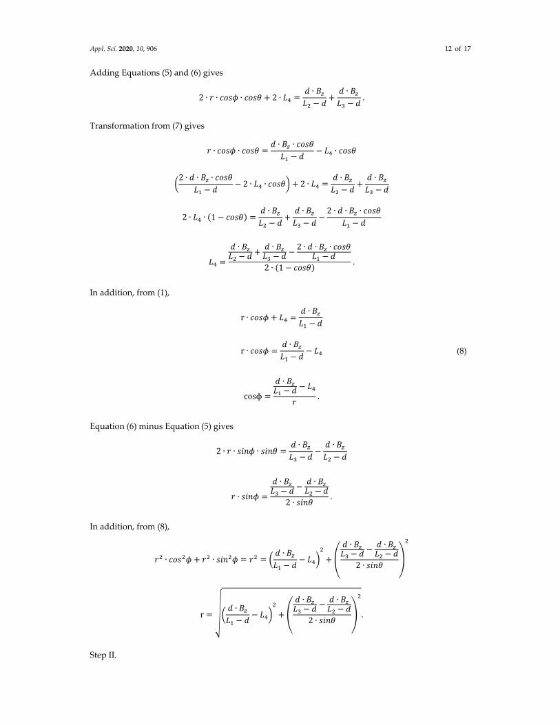
Step I.

𝑟 ∙ 𝑐𝑜𝑠𝜙 𝐿𝑟 ∙ 𝑐𝑜𝑠𝜙 𝐿 𝐵

𝑑𝐿 (1)

𝑟 ∙ 𝑐𝑜𝑠 𝜙 𝜃 𝐿𝑟 ∙ 𝑐𝑜𝑠 𝜙 𝜃 𝐿 𝐵

𝑑𝐿 (2)

𝑟 ∙ 𝑐𝑜𝑠 𝜙 𝜃 𝐿𝑟 ∙ 𝑐𝑜𝑠 𝜙 𝜃 𝐿 𝐵

𝑑𝐿 (3)

𝐿∙ ∙ ∙ ∙ ∙

∙ (θ cannot be zero and must be less than 90°)

Appl. Sci. 2020, 10, 906 11 of 17

r𝑑 ∙ 𝐵𝐿 𝑑

𝐿

⎣⎢⎢⎢⎡ 𝑑 ∙ 𝐵𝐿 𝑑

𝑑 ∙ 𝐵𝐿 𝑑

2 ∙ 𝑠𝑖𝑛𝜃

⎦⎥⎥⎥⎤

cosϕ

𝑑 ∙ 𝐵𝐿 𝑑 𝐿

𝑟

From (1),

𝑟 ∙ 𝑐𝑜𝑠𝜙 𝐿𝑟 ∙ 𝑐𝑜𝑠𝜙 𝐿 𝐵

𝑑𝐿

.

From (2),

r ∙ cosϕ ∙ 𝐿 𝐿 ∙ 𝐿 𝑟 ∙ 𝑐𝑜𝑠𝜙 ∙ d 𝐿 ∙ d d ∙ 𝐵 .

Multiply both sizes of the equation by :

𝑟 ∙ 𝑐𝑜𝑠𝜙 ∙ 𝐿 𝐿 ∙ 𝐿𝑟 ∙ 𝑐𝑜𝑠𝜙 ∙ 𝐿 𝐿 ∙ 𝐿 𝐿 ∙ 𝐵

𝑟 ∙ 𝑐𝑜𝑠𝜙 ∙ 𝑑 𝑑 ∙ 𝐿 𝑑 ∙ 𝐵𝑟 ∙ 𝑐𝑜𝑠𝜙 ∙ 𝐿 𝐿 ∙ 𝐿 𝐿 ∙ 𝐵

.

Simplify the denominator:

𝑟 ∙ 𝑐𝑜𝑠𝜙 ∙ 𝐿 𝐿 ∙ 𝐿 𝑟 ∙ 𝑐𝑜𝑠𝜙 ∙ 𝑑 𝑑 ∙ 𝐿 𝑑 ∙ 𝐵

r ∙ 𝑐𝑜𝑠𝜙 ∙ 𝐿 𝑑 𝐿 ∙ 𝑑 𝐿 𝑑 ∙ 𝐵 𝑑 ∙ 𝐵 𝐿 ∙ 𝐿 𝑑

𝑟 ∙ 𝑐𝑜𝑠𝜙 𝐿 ∙ 𝐿 𝑑 𝑑 ∙ 𝐵

𝑟 ∙ 𝑐𝑜𝑠𝜙 𝐿𝑑 ∙ 𝐵𝐿 𝑑

. (4)

Similarly, from (2),

r ∙ 𝑐𝑜𝑠 𝜙 𝜃 𝐿𝑑 ∙ 𝐵𝐿 𝑑

r ∙ 𝑐𝑜𝑠𝜙 ∙ 𝑐𝑜𝑠𝜃 𝑟 ∙ 𝑠𝑖𝑛𝜙 ∙ 𝑠𝑖𝑛𝜃 𝐿𝑑 ∙ 𝐵𝐿 𝑑

. (5)

Similarly, from (3),

r ∙ 𝑐𝑜𝑠 𝜙 𝜃 𝐿𝑑 ∙ 𝐵𝐿 𝑑

r ∙ 𝑐𝑜𝑠𝜙 ∙ 𝑐𝑜𝑠𝜃 𝑟 ∙ 𝑠𝑖𝑛𝜙 ∙ 𝑠𝑖𝑛𝜃 𝐿𝑑 ∙ 𝐵𝐿 𝑑

(6)

(4)*cosθ

r ∙ 𝑐𝑜𝑠𝜙 ∙ 𝑐𝑜𝑠𝜃 𝐿 ∙ 𝑐𝑜𝑠𝜃𝑑 ∙ 𝐵 ∙ 𝑐𝑜𝑠𝜃𝐿 𝑑

. (7)

Appl. Sci. 2020, 10, 906 12 of 17

Adding Equations (5) and (6) gives

2 ∙ 𝑟 ∙ 𝑐𝑜𝑠𝜙 ∙ 𝑐𝑜𝑠𝜃 2 ∙ 𝐿𝑑 ∙ 𝐵𝐿 𝑑


.

Transformation from (7) gives

𝑟 ∙ 𝑐𝑜𝑠𝜙 ∙ 𝑐𝑜𝑠𝜃𝑑 ∙ 𝐵 ∙ 𝑐𝑜𝑠𝜃𝐿 𝑑

𝐿 ∙ 𝑐𝑜𝑠𝜃

2 ∙ 𝑑 ∙ 𝐵 ∙ 𝑐𝑜𝑠𝜃𝐿 𝑑

2 ∙ 𝐿 ∙ 𝑐𝑜𝑠𝜃 2 ∙ 𝐿𝑑 ∙ 𝐵𝐿 𝑑


2 ∙ 𝐿 ∙ 1 𝑐𝑜𝑠𝜃𝑑 ∙ 𝐵𝐿 𝑑



𝐿




2 ∙ 1 𝑐𝑜𝑠𝜃 .

In addition, from (1),

r ∙ 𝑐𝑜𝑠𝜙 𝐿𝑑 ∙ 𝐵𝐿 𝑑

r ∙ 𝑐𝑜𝑠𝜙𝑑 ∙ 𝐵𝐿 𝑑

𝐿 (8)

cosϕ

𝑑 ∙ 𝐵𝐿 𝑑 𝐿

𝑟 .

Equation (6) minus Equation (5) gives

2 ∙ 𝑟 ∙ 𝑠𝑖𝑛𝜙 ∙ 𝑠𝑖𝑛𝜃𝑑 ∙ 𝐵𝐿 𝑑


𝑟 ∙ 𝑠𝑖𝑛𝜙



2 ∙ 𝑠𝑖𝑛𝜃 .

In addition, from (8),

𝑟 ∙ 𝑐𝑜𝑠 𝜙 𝑟 ∙ 𝑠𝑖𝑛 𝜙 𝑟𝑑 ∙ 𝐵𝐿 𝑑

𝐿



2 ∙ 𝑠𝑖𝑛𝜃

r𝑑 ∙ 𝐵𝐿 𝑑

𝐿



2 ∙ 𝑠𝑖𝑛𝜃.

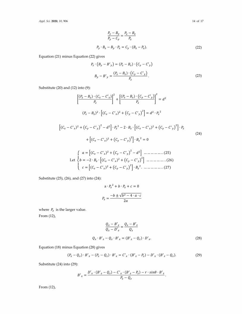
Step II.

Appl. Sci. 2020, 10, 906 13 of 17

𝐵 𝐵′ 𝐵 𝐵′ 𝑑 (9)

𝑃 𝐵′𝑃 𝐶′


𝑃 𝐵′𝑃 0

(10)

𝑃 𝐵𝑃 𝐶

𝑃 𝐵𝑃 𝐶

𝑃 𝐵𝑃 0

(11)

𝑄 𝐵′𝑄 𝐷′


𝑄 𝐵′𝑄 0

(12)

𝑄 𝐵𝑄 𝐷

𝑄 𝐵𝑄 𝐷

𝑄 𝐵𝑄 0

(13)

𝑄 𝑃 𝑟 ∙ 𝑠𝑖𝑛𝜃 (14)

𝑄 𝑃 (15)

𝑄 𝑃𝑟 ∙ 𝑠𝑖𝑛𝜃

𝑡𝑎𝑛 180 𝜃2

(16)

𝐵 𝐵′ (17)

Derivations:

From (10),


𝑃 𝐵′𝑃

𝑃 ∙ 𝐵 𝑃 ∙ 𝐵 𝐶 ∙ 𝐵 𝑃 . (18)

From (11),

𝑃 𝐵𝑃 𝐶

𝑃 𝐵𝑃

𝑃 ∙ 𝐵 𝑃 ∙ 𝐵 𝐶 ∙ 𝐵 𝑃 . (19)


𝑃 ∙ 𝐵 𝐵 𝑃 𝐵 ∙ 𝐶 𝐶′

𝐵 𝐵𝑃 𝐵 ∙ 𝐶 𝐶

𝑃 . (20)

From (10),


𝑃 𝐵′𝑃

𝑃 ∙ 𝐵 𝐵 ∙ 𝑃 𝐶 ∙ 𝐵 𝑃 . (21)

From (11),

Appl. Sci. 2020, 10, 906 14 of 17

𝑃 𝐵𝑃 𝐶

𝑃 𝐵𝑃

𝑃 ∙ 𝐵 𝐵 ∙ 𝑃 𝐶 ∙ 𝐵 𝑃 . (22)


𝑃 ∙ 𝐵 𝐵 𝑃 𝐵 ∙ 𝐶 𝐶′

𝐵 𝐵𝑃 𝐵 ∙ 𝐶 𝐶

𝑃 . (23)

Substitute (20) and (12) into (9):

𝑃 𝐵 ∙ 𝐶 𝐶′𝑃

𝑃 𝐵 ∙ 𝐶 𝐶′𝑃

𝑑

𝑃 𝐵 ∙ 𝐶 𝐶 𝐶 𝐶 𝑑 ∙ 𝑃

𝐶 𝐶 𝐶 𝐶 𝑑 ∙ 𝑃 2 ∙ 𝐵 ∙ 𝐶 𝐶 𝐶 𝐶 ∙ 𝑃

𝐶 𝐶 𝐶 𝐶 ∙ 𝐵 0

(24)

Let

⎩⎪⎨

⎪⎧ 𝑎 𝐶 𝐶 𝐶 𝐶 𝑑 … … … … … . . 25

𝑏 2 ∙ 𝐵 ∙ 𝐶 𝐶 𝐶 𝐶 … … … … … . . 26

𝑐 𝐶 𝐶 𝐶 𝐶 ∙ 𝐵 . … … … … … . . 27

Substitute (25), (26), and (27) into (24):

a ∙ 𝑃 𝑏 ∙ 𝑃 𝑐 0

𝑃𝑏 √𝑏 4 ∙ 𝑎 ∙ 𝑐

2𝑎

where 𝑃 is the larger value.

From (12),


𝑄 𝐵′𝑄

𝑄 ∙ 𝐵 𝑄 ∙ 𝐵 𝐵 𝑄 ∙ 𝐷 . (28)


𝑃 𝑄 ∙ 𝐵 𝑃 𝑄 ∙ 𝐵 𝐶 ∙ 𝐵 𝑃 𝐷 ∙ 𝐵 𝑄 . (29)

Substitute (24) into (29):

𝐵𝐷′ ∙ 𝐵 𝑄 𝐶 ∙ 𝐵 𝑃 𝑟 ∙ 𝑠𝑖𝑛𝜃 ∙ 𝐵

𝑃 𝑄 .

From (12),

Appl. Sci. 2020, 10, 906 15 of 17


𝑄 𝐵′𝑄

𝑄 ∙ 𝐵 𝑄 ∙ 𝐵 𝐵 𝑄 ∙ 𝐷 . (30)


𝑃 𝑄 ∙ 𝐵 𝑃 𝑄 ∙ 𝐵 𝐶 ∙ 𝐵 𝑃 𝐷 ∙ 𝐵 𝑄 . (31)

We then find 𝐵 :

𝐵𝐶 ∙ 𝐵 𝑃 𝐷 ∙ 𝐵 𝑄

𝑄 𝑃 .

Substitute 𝐵 into (20):

𝐵 𝐵𝑃 𝐵 ∙ 𝐶 𝐶′

𝑃 .


𝐵 𝐵𝑃 𝐵 ∙ 𝐶 𝐶′

𝑃 .


𝑃𝑃 ∙ 𝐵 𝐶′ ∙ 𝐵′ 𝑃

𝐵′ .


𝑃𝑃 ∙ 𝐵 𝐶′ ∙ 𝐵′ 𝑃

𝐵′ .

Author Contributions: Conceptualization, C.L. and J.H.; Data curation, M.T., Y.L. and J.H.; Formal analysis,

C.L.; Investigation, C.L. and J.H.; Methodology, C.L., H.H., L.F., Y.L., Z.S. and J.H.; Resources, L.F. and J.H.;

Supervision, J.H.; Validation, C.L.; Writing—original draft, C.L., M.T., H.H. and J.H.; Writing—review and

editing, J.H. All authors have read and agreed to the published version of the manuscript.

Funding: This study was partially supported by China Medical University (CMU108‐S‐01), Taiwan.

Conflicts of Interest: The authors declare no conflict of interest.

References

1. Fava, L.; Dummer, P. Periapical radiographic techniques during endodontic diagnosis and treatment. Int

Endod J 1997, 30, 250–261.

2. Vandenberghe, B.; Jacobs, R.; Bosmans, H. Modern dental imaging: a review of the current technology and

clinical applications in dental practice. Eur Radiol 2010, 20, 2637–2655, doi:10.1007/s00330‐010‐1836‐1.

3. Fu, H.‐M.; Chueh, H.‐S.; Tsai, W.‐K.; Chen, J.‐C.J.B.E.A. Development and evaluation of reconstruction

methods for an in‐house designed cone‐beam micro‐CT imaging system. Biomed. Eng. Appl. Basis Commun.

2006, 18, 270–275.

4. Kiljunen, T.; Kaasalainen, T.; Suomalainen, A.; Kortesniemi, M. Dental cone beam CT: A review. Physica

Med. 2015, 31, 844–860.

5. Pauwels, R.; Araki, K.; Siewerdsen, J.; Thongvigitmanee, S. Technical aspects of dental CBCT: state of the

art. Dentomaxillofacial Radiol. 2014, 44, 20140224.

6. Metsälä, E.; Henner, A.; Ekholm, M. Quality assurance in digital dental imaging: a systematic review. Acta

Odontol. Scand. 2014, 72, 362–371.

Appl. Sci. 2020, 10, 906 16 of 17

7. Patel, S.; Dawood, A.; Whaites, E.; Pitt Ford, T. New dimensions in endodontic imaging: part 1.

Conventional and alternative radiographic systems. Int Endod J 2009, 42, 447–462, doi:10.1111/j.1365‐

2591.2008.01530.x.

8. Liao, C.‐W.; Hsieh, C.‐J.; Huang, H.‐L.; Fuh, L.‐J.; Kuo, C.‐W.; Lin, Y.‐b.; Chen, J.‐C.; Hsu, J.‐T.J.B.E.A.

Prototype of a 2.5 D periapical radiography system using an intraoral computed tomosynthesis approach.

Biomed. Eng. Appl. Basis Commun. 2018, 30, 1850004.

9. Shan, J.; Tucker, A.; Gaalaas, L.; Wu, G.; Platin, E.; Mol, A.; Lu, J.; Zhou, O.J.D.R. Stationary intraoral digital

tomosynthesis using a carbon nanotube X‐ray source array. Dentomaxillofacial Radiol. 2015, 44, 20150098.

10. Inscoe, C.R.; Wu, G.; Soulioti, D.E.; Platin, E.; Mol, A.; Gaalaas, L.R.; Anderson, M.R.; Tucker, A.W.; Boyce,

S.; Shan, J. Stationary intraoral tomosynthesis for dental imaging. In Proceedings of Medical Imaging 2017:

Physics of Medical Imaging, Orlando, Florida, United States, March 2017; p. 1013203.

11. Inscoe, C.R.; Platin, E.; Mauriello, S.M.; Broome, A.; Mol, A.; Gaalaas, L.R.; Regan Anderson, M.W.; Puett,

C.; Lu, J.; Zhou, O.J.M.p. Characterization and preliminary imaging evaluation of a clinical prototype

stationary intraoral tomosynthesis system. Med. Phys. 2018, 45, 5172–5185.

12. Liao, C.‐W.; Huang, K.‐J.; Chen, J.‐C.; Kuo, C.‐W.; Wu, Y.‐Y.; Hsu, J.‐T. A Prototype Intraoral Periapical

Sensor with High Frame Rates for a 2.5 D Periapical Radiography System. Appl. Bionics Biomech. 2019, 2019,

doi: https://doi.org/10.1155/2019/7987496.

13. Xiang, Q.; Wang, J.; Cai, Y. A geometric calibration method for cone beam CT system. In Proceedings of

Eighth International Conference on Digital Image Processing (ICDIP 2016), Chengu, China, 2016; p.

100333G.

14. Zhao, J.; Hu, X.; Zou, J.; Hu, X.J.S. Geometric parameters estimation and calibration in cone‐beam micro‐

CT. Sens. 2015, 15, 22811–22825.

15. Johnston, S.M.; Johnson, G.A.; Badea, C.T.J.M.p. Geometric calibration for a dual tube/detector micro‐CT

system. Med. Phys. 2008, 35, 1820–1829.

16. Von Smekal, L.; Kachelrieß, M.; Stepina, E.; Kalender, W.A.J.M.p. Geometric misalignment and calibration

in cone‐beam tomography: Geometric misalignment and calibration in cone‐beam tomography. Med. Phys.

2004, 31, 3242–3266.

17. Li, L.; Yang, Y.; Chen, Z.J.O.E. Geometric estimation method for x‐ray digital intraoral tomosynthesis. Opt.

Eng. 2016, 55, 063105.

18. Richard L. Webber, W.‐S. Self‐calibrated tomosynthetic, radiographic‐imaging system, method, and device.

U.S. Patent No 5,359,637, 25 October 1994.

19. Yang, Y.; Li, L.; Chen, Z.; Chang, M. Geometrical calibration method for x‐ray intra‐oral digital

tomosynthesis. In Proceedings of 2014 IEEE Nuclear Science Symposium and Medical Imaging Conference

(NSS/MIC), Seattle, WA, USA, 2014; pp. 1–4.

20. Li, L.; Chen, Z.; Zhao, Z.; Wu, D. X‐ray digital intra‐oral tomosynthesis for quasi‐three‐dimensional

imaging: system, reconstruction algorithm, and experiments. Opt. Eng. 2013, 52, 013201.

21. Sato, K.; Ohnishi, T.; Sekine, M.; Haneishi, H. Geometry calibration between X‐ray source and detector for

tomosynthesis with a portable X‐ray system. Int. J. Comput. Assisted Radiol. Surg. 2017, 12, 707–717.

22. Miao, H.; Wu, X.; Zhao, H.; Liu, H. A phantom‐based calibration method for digital x‐ray tomosynthesis.

J. X‐Ray Sci. Technol. 2012, 20, 17–29.

23. Chtcheprov, P.; Hartman, A.; Shan, J.; Lee, Y.Z.; Zhou, O.; Lu, J. Optical geometry calibration method for

free‐form digital tomosynthesis. In Proceedings of Medical Imaging 2016: Physics of Medical Imaging, San

Diego, California, United States, 2016; p. 978365.

24. Fayad, M.I.; Nair, M.; Levin, M.D.; Benavides, E.; Rubinstein, R.A.; Barghan, S.; Hirschberg, C.S.; Ruprecht,

A. AAE and AAOMR joint position statement: use of cone beam computed tomography in endodontics

2015 update. Oral Surg. Oral Med. Oral Pathol. Oral Radiol. 2015, 120, 508–512.

25. Hayakawa, Y.; Yamamoto, K.; Kousuge, Y.; Kobayashi, N.; Wakoh, M.; Sekiguchi, H.; Yakushiji, M.;

Farman, A. Clinical validity of the interactive and low‐dose three‐dimensional dento‐alveolar imaging

system, Tuned‐Aperture Computed Tomography. Bull. Tokyo Dent. Coll.2003, 44, 159–167.

26. Groenhuis, R.A.; Webber, R.L.; Ruttimann, U.E.J.O.S. Computerized tomosynthesis of dental tissues. Oral

Med. Oral Pathol. 1983, 56, 206–214.

27. Grant, D.G. Tomosynthesis: a three‐dimensional radiographic imaging technique. IEEE Trans. Biomed. Eng.

1972, 1, 20–28.

Appl. Sci. 2020, 10, 906 17 of 17

28. Ziegler, C.M.; Franetzki, M.; Denig, T.; Muhling, J.; Hassfeld, S. Digital tomosynthesis‐experiences with a

new imaging device for the dental field. Clin. Oral Invest. 2003, 7, 41–45. doi:10.1007/s00784‐003‐0195‐6.

29. Rashedi, B.; Tyndall, D.A.; Ludlow, J.B.; Chaffee, N.R.; Guckes, A. Tuned aperture computed tomography

(TACT®) for cross‐sectional implant site assessment in the posterior mandible. J. Prosthodontics 2003, 12,

176–186.

30. Harase, Y.; Araki, K.; Okano, T. Diagnostic ability of extraoral tuned aperture computed tomography

(TACT) for impacted third molars. Oral Surg. Oral Med. Oral Pathol. Oral Radiol. Endodontology 2005, 100,

84–91.

31. Limrachtamorn, S.; Edge, M.; Gettleman, L.; Scheetz, J.; Farman, A. Array geometry for assessment of

mandibular implant position using tuned aperture computed tomography (TACT™). Dentomaxillofacial

Radiol. 2004, 33, 25–31.

32. Harase, Y.; Araki, K.; Okano, T. Accuracy of extraoral tuned aperture computed tomography (TACT) for

proximal caries detection. Oral Surg. Oral Med. Oral Pathol. Oral Radiol. Endodontology 2006, 101, 791–796.

33. Yang, K.; Kwan, A.L.; Miller, D.F.; Boone, J. A geometric calibration method for cone beam CT systems.

Med. Phys. 2006, 33, 1695–1706.

34. Sun, Y.; Hou, Y.; Zhao, F.; Hu, J. A calibration method for misaligned scanner geometry in cone‐beam

computed tomography. NDT E Int. 2006, 39, 499–513.

35. Wang, X.; Mainprize, J.G.; Kempston, M.P.; Mawdsley, G.E.; Yaffe, M.J. Digital breast tomosynthesis

geometry calibration. In Proceedings of Medical Imaging 2007: Physics of Medical Imaging, San Diego, CA,

United States, 2007; p. 65103B.

36. Claus, B.E.H.; Opsahl‐Ong, B.; Yavuz, M. Method, apparatus, and medium for calibration of tomosynthesis

system geometry using fiducial markers with non‐determined position. U.S. Patent No. 6,888,924. 3 May

2005.

© 2020 by the authors. Licensee MDPI, Basel, Switzerland. This article is an open access

article distributed under the terms and conditions of the Creative Commons Attribution

(CC BY) license (http://creativecommons.org/licenses/by/4.0/).

Geometrical Calibration of a 2.5D Periapical Radiography ...

Documents

Transcript of Geometrical Calibration of a 2.5D Periapical Radiography ...