A geometrical approach for inverting display color-characterization models

A geometrical approach for inverting display color-characterization models

Jean-Baptiste ThomasPhilippe ColantoniJon Y. HardebergIrène FoucherotPierre Gouton

Abstract — Some display color-characterization models are not easily inverted. This work proposesways to build geometrical inverse models given any forward color-characterization model. The maincontribution is to propose and analyze several methods to optimize the 3-D geometrical structure ofan inverse color-characterization model directly based on the forward model. Both the amount of dataand their distribution in color space is especially focused on. Several optimization criteria, relatedeither to an evaluation data set or to the geometrical structure itself, are considered. A practical casewith several display devices, combining the different methods proposed in the article, are consideredand analyzed.

Keywords — Display device, color characterization, inverse model, geometrical structure, 3-D look-up table, interpolation, data distribution, optimization.

DOI # 10.1889/JSID16.10.1021

1 IntroductionThe goal of color characterization of display devices is todefine the relationship between the device-dependent colorspace, typically RGB, and a device-independent color space,typically CIEXYZ or CIELAB, based on a standard CIE col-orimetric observer describing the perceived color.1 Thisrelationship has two directions. The forward transformationaims to predict the displayed color for any set of digital val-ues input to the device, i.e., a triplet (dr, dg, db). The inversetransformation provides the set of digital values to input tothe device in order to display a desired color.

Among the models or methods used to achieve colorcharacterization, we can distinguish two categories. Thefirst one contains models that are analytically invertible,2–8

such as the PLCC (piecewise linear assuming chromaticityconstancy), the black corrected PLCC*, the GOG (gain-off-set–gamma) or GOGO (gain-offset–gamma-offset) models.The second category contains the models or methods whichare not analytically invertible. Models of this second cate-gory require other methods to be inverted. We can list sometypical problems and methods used to invert these models:

� A condition has to be verified, such as in the mask-ing model.9

� A new matrix might have to be defined by regres-sion in numerical models.10,7,8,11

� A full optimization process has to be set up for eachcolor, such as in S-curve model II,12,13 in the modi-fied masking model,9 or in the PLVC (piecewise lin-ear assuming variation in chromaticity) model.3,6

� The optimization process can appear only for onestep of the inversion process, as in the PLVC3 or inthe S-curve I12,13 models.

� Empirical methods based on 3-D LUT (lookup table)can be inverted directly,14 using the same geometri-cal structure. In order to have a better accuracy,however, it is common to build another geometricalstructure to yield the inverse model. For instance, itis possible to build a draft model to define a new setof color patches to be measured.15

The computational complexity required to invertthese models makes them seldom used in practice, exceptthe full 3-D LUT whose major drawback is that it requiresa lot of measurements. However, these models do have thepossibility to take into account more precisely the devicecolor-reproduction features, such as interaction betweenchannels or chromaticity inconstancy of the primaries.Thus, they are often more accurate than the models of thefirst category.

Given any of these models, we propose here to build ageometrical inverse model based on an optimized tetrahe-dral structure generated from the forward model, such thatno more measurements than the ones needed to set up theforward model are required.

The main contribution of this work is to propose anddiscuss some algorithms allowing the establishment of theoptimized geometrical structure of such an inverse model.This work follows and completes a preliminary study whichhas been presented earlier.16 Two main grid features arestudied, as well as the number of points used and their dis-tribution.

In the following, we first introduce our general frame-work, modeling the problem and introducing notations. Wethen propose several methods to optimize both the numberand the distribution of data used to build this inverse model.

J-B. Thomas is with the Norwegian Color Research Laboratory, Gjøvik University College, Gjøvik, Norway, and the Université de Bourgogne, Le2i, 9av. Alain Savary, Djion, Bourgogne 21078, Dijon, France; telephone +47-611-40426, fax –35240, e-mail: [email protected].

J. Y. Hardeberg is with the Norwegian Color Research Laboratory, Gjøvik University College, Gjøvik, Norway.

P. Colantoni is with the Centre de Recherche et de Restauration des musées de France, Paris, France.

I. Foucherot and P. Gouton are with the Université de Bourgogne, Dijon, France.

© Copyright 2008 Society for Information Display 1071-0922/08/1610-1021$1.00

Journal of the SID 16/10, 2008 1021

Finally, we present results on the inversion of the PLVCforward model applied to several display devices.

2 Background workBuilding an inverse color-charaterization model based on a3-D LUT is not new. Such a model is defined by the numberand the distribution of the color patches used in the LUT,and on the interpolation method used to generalize themodel to the entire space. In this section, we review somebasic tools and methods. We distinguish between works ondisplays and more general works which have been per-formed in this way either in a general purpose or especiallyfor printers. We present in detail the tetrahedral structurewe used as a basis of our work. Our method to obtain theinverse model is based on the use of a forward model and onthe refinement of the grid in the destination space ratherthan in the source space. We have chosen the PLVC modelas forward transform, which is described in the second partof this section.

2.1 Building an inverse model based on a3-D LUT

3-D LUT inverse models in displays are often based on themeasurement of a defined number of color patches, i.e., weknow the transformation between CIELAB and RGB in asmall number of color-space locations. Then, this transfor-mation is generalized to the entire color space by interpola-tion. Previous studies assess that these methods achievegood results for display devices,14,15 depending on the com-bination of the interpolation method used,17,24–26,22 thenumber of patches measured, and on their distribution15

(some of the interpolation methods cited above cannot beused with a non-regular distribution). However, to be pre-cise enough, a lot of measurements are typically required,e.g., a 10 × 10 × 10 grid of patches measured in Bastani’spaper.14 Note that such a model is technology independentsince no assumption is made about the device, only that thedisplay will always have the same response as at the meas-urement location, i.e., that it is spacially uniform. Such amodel needs high storage capacity and computational powerto handle the 3-D data. The computational power is usuallynot a problem since graphic processor units (GPU) can per-form this type of task easily today. The high number of meas-urements needed is a greater challenge.

The problem of measurement is even more restrictivefor printers and many works have been carried out in usinga 3-D LUT for the color characterization of these devices.Moreover, since printer devices are highly non-linear, theircolorimetric models are complexe, and it has been custom-ary in the last decade to use a 3-D complex LUT for theforward model, created by using an analytical forwardmodel; both to reduce the amount of measurement and toperform the color-space transform in a reasonable time. Thefirst work we know about creating a LUT based on the for-

ward model is a patent from Stokes.27 In this work, the LUTis built to replace the analytical model in the forward direc-tion. It is based on a regular grid designed in the printerCMY color space, and the same LUT is used in the inversedirection, simply in switching the domain and co-domain.Note that in displays, the forward model is usually compu-tationally simple and that we need only to use a 3-D LUTfor the inverse model. The uniform mapping of the CMYspace leads to a non-uniform mapping in CIELAB space forthe inverse direction, and it is common now to re-samplethis space to create a new LUT. To do that, a new grid isusually designed in CIELAB and is inverted after gamutmapping of the point located outside the gamut of theprinter. Several algorithms can be used to re-distribute thedata28–30 and to fill the grid.31–33

Returning to displays, let us call source space the inde-pendent color-space CIELAB (or either CIEXYZ), the domainfrom where we want to move and destination space, theRGB color space, the co-domain, where we want to move to.If we want to build a grid, we then have two classicalapproaches to distribute the patches in the source space,using the forward model. One can use directly a regular dis-tribution in RGB and transform it to CIELAB using thefoward model; this approach is the same as used by Stokesfor printers,27 and leads to a non-uniform mapping of theCIELAB space which leads to inaccuracy for the inversedirection. An other approach can be to distribute thepatches regularly in CIELAB, following a given pattern, forinstance following Stauders15 for an hexagonal structure orany of the methods used in printers.28–30 Then, an optimi-zation process using the forward model can be performedfor each point to find the corresponding RGB value.

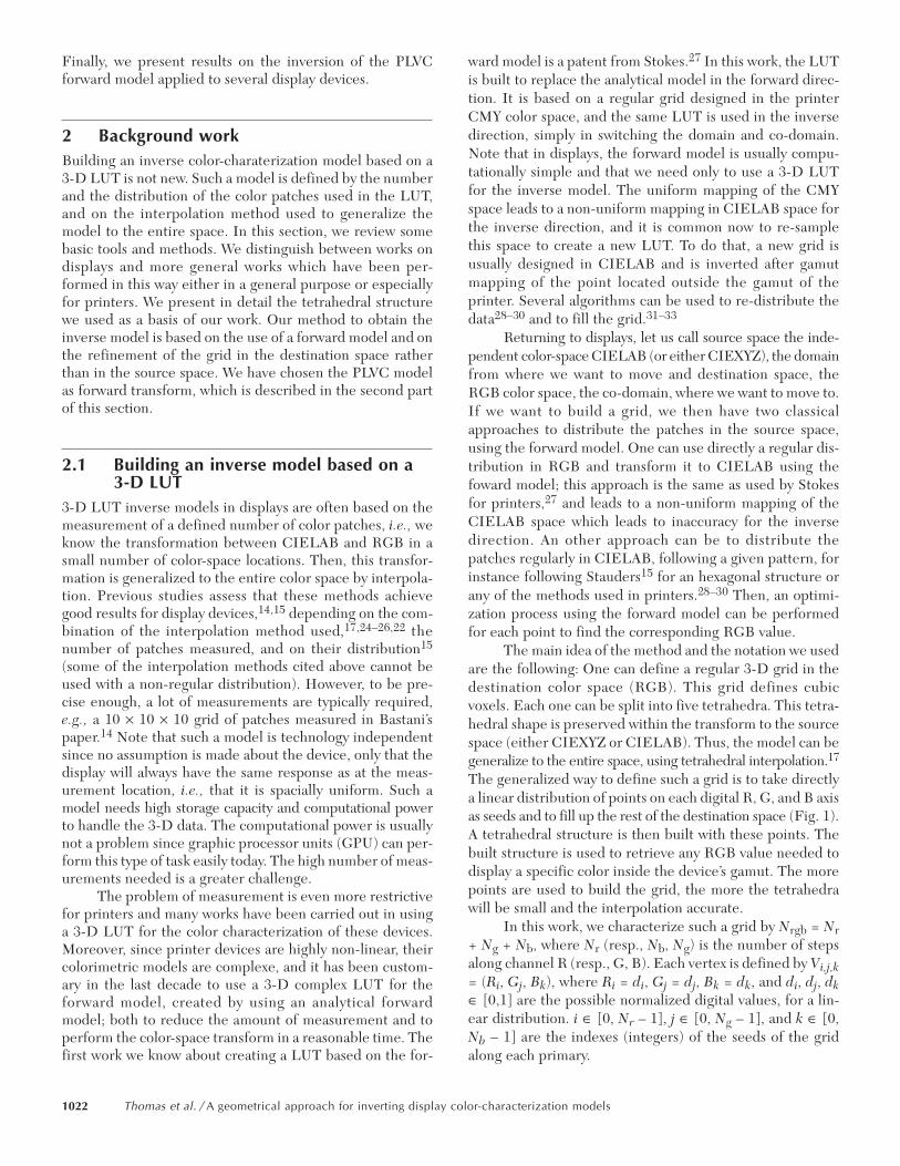
The main idea of the method and the notation we usedare the following: One can define a regular 3-D grid in thedestination color space (RGB). This grid defines cubicvoxels. Each one can be split into five tetrahedra. This tetra-hedral shape is preserved within the transform to the sourcespace (either CIEXYZ or CIELAB). Thus, the model can begeneralize to the entire space, using tetrahedral interpolation.17

The generalized way to define such a grid is to take directlya linear distribution of points on each digital R, G, and B axisas seeds and to fill up the rest of the destination space (Fig. 1).A tetrahedral structure is then built with these points. Thebuilt structure is used to retrieve any RGB value needed todisplay a specific color inside the device’s gamut. The morepoints are used to build the grid, the more the tetrahedrawill be small and the interpolation accurate.

In this work, we characterize such a grid by Nrgb = Nr+ Ng + Nb, where Nr (resp., Nb, Ng) is the number of stepsalong channel R (resp., G, B). Each vertex is defined by Vi,j,k= (Ri, Gj, Bk), where Ri = di, Gj = dj, Bk = dk, and di, dj, dk∈ [0,1] are the possible normalized digital values, for a lin-ear distribution. i ∈ [0, Nr – 1], j ∈ [0, Ng – 1], and k ∈ [0,Nb – 1] are the indexes (integers) of the seeds of the gridalong each primary.

1022 Thomas et al. / A geometrical approach for inverting display color-characterization models

Once this grid has been built, we define the tetrahe-dral structure for the interpolation following Kasson et al.17

Then we use the forward model to transform the structureinto CIELAB colorspace (see Fig. 2). We have built aninverse model.

According to the non-linearity of the CIELAB trans-form, the size of the tetrahedra is not anymore the same asit was in RGB. In the following section, we propose to mod-ify this framework to make this grid more homogeneous inthe source color space where we perform the interpolation,this should lead to a better accuracy, following Ref. 29.

2.2 The PLVC modelThe forward model we used in this work is the piecewiselinear assuming variation in chromaticity (PLVC). Thismodel has been introduced first by Farley and Gutmann19

in 1980. Post and Calhoun3 have performed a study of thismodel on CRT technology. Del Barco et al.6 have proposeda modification of this model including a black correction.Other studies has been performed on different display tech-nologies.20,21,23 This model does not consider the channelinter-dependence, but models the chromaticity shift of theprimaries. In this section we present this model and the fea-tures which characterize it.

Knowing the tristimulus values X, Y, and Z for eachprimary as a function of the digital input, assuming additiv-ity, the resulting color tristimulus values can be expressed asthe sum of tristimulus values for each component (i.e., pri-mary) at the given input level. The black level is removedfrom all measurements which define the model in order not

to include it several times and is added back at the end toreturn to a correct standard observer color space.6,20 Themodel is summarized and generalized in Eq. (1) for N pri-maries and illustrated in Eq. (2) for a three primaries RGBdevice, following an equivalent formulation as the one givenby Jimenez del Barco et al.6

For an N primaries device, we consider the digitalinput to the i-th primary, di(mi), with i an integer ∈ [0, N],and mi an integer limited by the resolution of the device(i.e., mi ∈ [0,255] for a channel coded on 8 bits). Then, acolor XYZ(...,di(mi),...) can be expressed by

(1)

with Xk, Yk, Zk the N-tuplet defined by a (0,...,0) input.We illustrate this for a three-primary RGB device,

with each channel coded on 8 bits. The digital input aredr(i), dg(j), db(l), with i, j, l integers ∈ [0,255]. In this case,a XYZ[dr(i), dg(j), db(l)] can be expressed by

(2)

Previous studies of this model have shown good results,especially on dark and mid-luminance colors. When the col-ors reach higher luminances, the additivity assumption isless true for CRT technology. Then the accuracy decreases(depending on the device properties). More precisely, Postand Calhoun3,20 stated that chromaticity error is lower forthe PLVC than for the PLCC in low luminances. This is dueto the setting of primary chromaticities at maximumintensity in the PLCC. Both models show inaccuracy for

X d m X d j X X

Y d m Y d j Y Y

Z d m Z d j Z Z

i i i k ki j m

i N

i i i k ki j m

i N

i i i k ki j m

i N

i

i

i

( , ( ), ) [ ( ( )) ] ,

( , ( ), ) [ ( ( )) ] ,

( , ( ), ) [ ( ( )) ] ,

,

,

,

K K

K K

K K

= - +

= - +

= - +

= =

= -

= =

= -

= =

= -

Â

Â

Â

0

1

0

1

0

1

X d i d j d l X d i X X d j X

X d l X X

Y d i d j d l Y d i Y Y d j Y

Y d l Y Y

Z d i d j d l Z d i Z Z d j Z

Z d l Z Z

r g b r k g k

b k k

r g b r k g k

b k k

r g b r k g k

b k k

( ( ), ( ), ( )) [ ( ( )) ] [ ( ( )) ]

[ ( ( )) ] ,

( ( ), ( ), ( )) [ ( ( )) ] [ ( ( )) ]

[ ( ( )) ] ,

( ( ), ( ), ( )) [ ( ( )) ] [ ( ( )) ]

[ ( ( )) ] ,

= - + -

+ - += - + -

+ - += - + -

+ - +

FIGURE 1 — Design of a regular grid Nrgb = 24 in RGB.

FIGURE 2 — Tetrahedral structure based on a regular grid, Nrgb = 15 inRGB (left) and its transform in CIELAB (right).


high luminance colors due to channel inter-dependence.Jimenez del Barco et al.6 found that for CRT technology, thehigher level of brightness in the settings leads to a non-neg-ligible amount of light for a (0,0,0) input. This light shouldnot be added three times, and they proposed a correctionfor that. They found that the PLVC model was more accu-rate in medium-to-high luminance colors. Inaccuracy ismore important in low luminances, due to inaccuracy ofmeasurements, and in high luminances, due to channeldependencies. These results are generalized for other tech-nologies in Ref. 23.

The inversion of this model is more troublesome thanfor matrix-based models such as the PLCC. For a three-pri-mary display, according to Post and Calhoun,3 it can be per-formed, defining all subspaces defined by the matrices ofeach combination of measured data (the intercepts have tobe subtracted, and once all the contributions are known,they have to be added). It is also possible to perform anoptimization process for each color6 or to define a grid inRGB which will allow us to perform the inversion using 3-Dinterpolation. Note that Post and Calhoun have proposed todefine a full LUT considering all colors. They stated them-selves that it is inefficient. With the method proposed in thispaper, we are able to define an optimized reduced grid inRGB which will allow us to inverse this model.

3 Method proposedBeginning with a regular grid in the destination space, ourgoal is to transform this regular cubic structure into a rec-tangular one, in order to make it more uniform or better inthe source space. We propose to approximate an homogene-ous grid in the source space using only a few number ofparameters. Note that this approach ressembles, but differsfrom the existing methods in the way that we do not modifythe grid in the source space but directly and firstly in thedestination space. This leads to some differences: first, nogamut mapping is required to map the points which rise upoutside the gamut during the creation of a grid in the sourcespace. Secondly, the grid is taken in its globality and we willnot reach a perfect uniformity in the source space, only arough approximation of it, depending on the function weuse. Thirdly, the order between data is preserved, whichleads to an easier indexation of the tetrahedra.

In order to build a more uniform grid in the sourcecolor space, we propose to assume that

� The number of steps has not necessarily to be thesame along each primary in the destination space,then Nr ≠ Ng ≠ Nb.

� The steps have not to be regularly spaced along aprimary in the destination space, but they can bedefined such as Ri = fr(di), Gj = fg(dj), Bk = fb(dk).Considering f ∈ {fr, fg, fb}, a monotonically increas-ing function from R to R,

(3)

f could be any simple function, either a power function withone constant parameter or an S-shaped curve function withone to three constant parameters. Let us say that this func-tion has M parameters, then the number of parameters usedto set-up the distribution of the grid points is P = 3 × M.

We make the hypothesis that if we can find the goodfunction f, and the good number of steps, different for eachprimaries, the structure defined by the 3-D grid will becomemore homogeneous in the source space and will allow us tohave a better inversion map. By extension, we assess that ifwe can build a “better” grid in the source space, the inver-sion will become better. The purpose of the next subsectionis to define what a better grid is.

3.1 Estimation of the grid qualityA better grid can be defined in various ways. The straight-forward way to assume that a grid is better is to assume thatit is more regular in the source space, then some geometri-cal indicators should be used as cost functions to estimatethe function f. It could also be a structure well designed fora given application, then an evaluation data set could berequired. For a given number of steps along each channel,we have P values to optimize. The optimization processenables us to re-distribute the steps in the destination space,so we adapt the tetrahedral structure in the source space.We propose below three criteria as cost functions. One isdirectly linked with the geometrical structure of the grid.Others are linked to the result of the inverse model for anevaluation set of patches.

3.1.1 Criterion defined by the geometricalproperties of the structure

The first type of cost functions we consider contains thefunctions directly characterizing the geometry of the grid.The one we have used is the variance of the length of thetetrahedron’s edges of the geometrical structure in thesource space. If we minimize this function, the tetrahedronof the grid will have more or less the same shape. Using thiscriterion, we want to reduce the heterogeneity of the inter-polation error throughout the space, and so to minimize theerror of the model. We call this criterion “Edges” in thefollowing.

3.1.2 Criterion linked with an evaluationdata set

The cost functions of the second type affect the structureindirectly. We used an evaluation data set and tried to mini-mize either the maximum error or the average error of themodel for this data set. The evaluation data were 100 meas-

fd f d

:[0, ] [0, ]

( ).

1 1ÆÆ

RST


ured patches equiprobably distributed in the destinationspace. We call the two criteria “Mean” and “Max” in thefollowing.

A remark has to be done first about the choice of theevaluation data set. As the data are distributed in the desti-nation space, they are not well distributed in the sourcespace. That means that these indicators are not trying tohomogenize the grid in the source space. If the goal is tohomogenize the grid in the source space, then the data sethas to be equiprobably distributed in this space. However,minimizing the feature for an evaluation data set optimizesthe grid for instance for a special type of images or for asequence of a movie for one given device.

A second important thing to notice here is that even ifthe color of the training (or evaluation) data set belongs tothe gamut of the device, since they are defined in RGB, it isnot obvious that it belongs to the gamut defined by the for-ward model (see Fig. 3). Indeed, due to the forward model’sfailure, some colors could be out of the grid; thus, a gamutmapping is required. For instance, if the forward modeldoes not take into account interaction between channels,some colors could have more (or less) luminance than theforward model can predict and then be outside of the grid.

In our previous study16 we noticed that the optimiza-tion algorithm was trying to refine the grid around thesecolors where, for some displays, a critical maximum errorwas coming from the mapping of a color from the evaluationdata set. This effect appears especially for the “Max” criteria.

Since the model and the features seem not to bedirectly related with a derivable function, we have chosen anumerical optimization method. We used the globalizedNelder–Mead simplex downhill algorithm.18 This fits wellwith our problem, and we can use it easily with P variablesto optimize. Let us notice that criteria = G(p) is the functionto minimize, with p a vector of dimension P.

To give an exemple, let us consider Nrgb = 15, Nr = Ng= Nb = 5, in minimizing the aforementioned functions, wecan retrieve the best parameters α, β, γ of a power function,respectively, for each channel R, G, B, which will allow todefine our definitive structure (p = [α, β, γ]). In Fig. 4, thecost function “mean” has been used, and the results obtained

are a mean error of 4.13% and a maximum error of 18.83%in RGB, for a testing data set of 100 patches, while the origi-nal regular grid with the same number of patches gives amean error of 4.50% and a maximum error of 20.79%.

3.2 Distribution of the grid seedsIn this section, we first discuss the functions we used tomodify the distribution of the grid seeds along the R, G, andB axis, with an equal number of data for each axis. We thendiscuss the number of points that should be used along eachaxis, considering that these numbers could be different. Weseparated these steps in two different algorithms to see theinfluence of each of these. Both are then combined in apractical case in Sec. 4.

3.2.1 Static changing of the grid morphologyTo redistribute the grid seeds along each channel, we usedeither a simple power function or an S-shaped curve. Forboth cases, we have fixed the condition Nr = Ng = Nb, inorder to limit the number of parameters and for modelingpurpose. Let us investigate on the criterion used to find thefunction parameters and on the value of Nrgb.

� Power function: the grid seeds are expressed as Ri =di

α, Gj = djβ, Bk = dk

γ. As our digital values are nor-malized, the power function follows the requirementsdefined in Eq. (3). There are three parameters tooptimize.

� S-shaped curve function: the grid seeds are expressedas

if elsed Rd

Rd

i ii

ii< = = -

-0 5

22

12 1

2. ,

( ),

( ),

a a

if elsed Gd

Gd

j jj

jj

< = = --

0 52

21

2 1

2. ,

( ),

( ),

b b

if elsed Bd

Bd

k kk

kk< = = -

-0 5

22

12 1

2. ,

( ),

( ),

g g

FIGURE 3 — The gamut generated with the PLVC forward model doesnot correspond exactly with the device gamut. Then some colors insidethe true device gamut have to be mapped inside the geometricalstructure to be transformed into RGB values. On these figures, one cansee that some measured colors defined by some RGB values does notbelong to the gamut defined by the forward model.

FIGURE 4 — Tetrahedral structure based on a regular grid, Nrgb = 15and α = 1.23, β = 1.27, γ = 1 obtained for the criterion “mean” in RGB(left) and its transform in CIELAB (right).


such that the curve stays inside [0,1]. There are as well threeparameters to optimize.

Note that we have chosen a simple expression for thesigmoid, in order to have only one parameter for each chan-nel to optimize. This reduces the freedom of the function,but makes the method easier to explain and understand.

Let’s illustrate the method. Using a power function,the grid is defined by Nrgb and by the optimization of α, β,γ values. Figure 4 illustrates this construction for Nrgb = 15,i.e., Nr = Nr = Nr = 5. Using the criterion “Mean,” we foundα = 1.23, β = 1.27, γ = 1.

3.2.2 Spreading of the grid seedsAn equal number of steps along each R, G, and B channel isnot sufficient a priori to reach the homogeneity in CIELAB,even if they are not distributed linearly. Thus, we propose asecond way to build the geometrical structure which con-sists in distributing the steps along each channel in the bestway whitout the condition Nr = Ng = Nb. We used a bruteforce approach for this task. Given a number of points, wetried the possibilities sequentially such as Nrgb = Nr + Ng +Nb and we selected the best combination, considering thechosen cost function. To study the effect independently ofthe previous proposition, we distributed in a first time thesteps regularly along each channel.

4 ResultsWe have defined two ways to build a geometrical structureconsidering a given criterion. One is based on the staticchanging of the morphology of the grid in the destinationspace. The other focuses on the number of steps along eachaxis in the destination space. In this section, we present theresults obtained for each method developped to study theinfluence of both distributions. We study these methods infunction of the total number of steps used to build the grid.We then present a practical case where the two methods arecombined to build the best geometrical structure consider-ing the distribution of the points in the destination space fora given number of points and for a given criterion. In orderto analyze the results, we have chosen one forward model,the PLVC which assumes independence between channels,but takes into account the chromaticity shift of primaries.This model has been presented in Sec. 2. Results and analy-sis considering this model in the forward direction and forthe displays we tested can be found in Ref. 23. For the for-ward model, the Ak, A ∈ {X, Y, Z}, were obtained by accuratemeasurement of the black level. In this work, the [A(di(j)) –Ak], were obtained using Akima spline interpolation22 withthe measurement of a ramp along each primary. Note thatany 1-D interpolation can be used.

Practically, we used a bounding box centered on thecolor we wanted to display to determine the tetrahedron itbelongs to. Then a linear tetrahedral interpolation is per-formed.17 In the case of a point out of the grid, i.e., out of

gamut, we performed a simple clipping toward the 50%luminance. Since our data set is defined in RGB, the gamutclipping happens only when the forward model fails.

We show and discuss results obtained for the inversionof the PLVC model. We tested the algorithms on three dis-plays, a tri-LCD projector 3M-X50 (PLCD), a CRT monitorPhilips 107s (MCRT), and a LCD monitor DELL 1905FP(MLCD). The measurements of the color patches weretaken using the spectroradiometer CS-1000 from Minolta.

4.1 Static changing of the grid morphologyThis part discusses results with the first method proposed inSec. 3.2. We consider an equal number of steps along eachprimary, and we distribute them using a function whichparameters were found using an optimization process. InFig. 5, one can see the evolution of the accuracy of themodel in function of the number of steps used. All combi-nations between the functions and the criterion used arepresented. The reference is the regular grid.

In general, it is hard to say that one criterion com-bined with one type of function performs much better thanthe other possibilities.

The criterion “Edges” does not seem to give reallygood results neither in average nor in maximum error exceptfor the CRT display when it is combined with the S-shapedcurve. It is possible that this is the result of the testing dataset which was equiprobably spreaded in RGB.

For PLCD [Fig. 5(a)], criteria based on a training dataset gives equal or better results than the regular grid, gen-erally following the cost function used. However, one cansee that the combination of the criterion “Max“ and a powerfunction gives a good compromise in both the average andmaximum error for this display. This combination performsbetter than a regular grid. The difference is major for a reducedgrid; for instance, with Nrgb = 30, the regular grid gives anaverage error of about 1.5%, the “Edges” criterion an errorof 2% to over 3% depending on the function used, while allthe other methods with the “Mean” and the “Max” criteriagive an average error of 1–1.5%. If we look at the maximumerror for the same Nrgb, the regular grid gives an error over6.5%, the refinement of the grid using the training data setgives an error of 3–4%. That means that we reduced themaximum error by a factor of two for this case. The criterion“Edges” gives a maximum error higher than the error of theregular grid.

For MLCD [Fig. 5(b)], we notice the fast convergenceof the maximum error for all methods (the regular gridincluded). This is possibly due to the gamut mapping due tothe failure of the forward model. For this device and Nrgb =30, we notice that the sigmoid used gives better results thanthe regular grid (from around 3–2.6%) whatever the “Max”or “Mean” criterion we used.

MCRT [Fig. 5(c)] shows that, on this device, the regu-lar grid gives better results than the others and that “Edges”criterion seems to perform well on it, combined with a S-


curve. However, if we look at the results for Nrgb = 45, thesigmoid combined with the criteria based on the trainingdata set gives better results, reducing the error from 3% to2.4 and 2.5%.

When the number of points increases, all methodsseem to converge. All are going towards the same accuracy.Note that the “Edges” criterion combined with a power-shapedcurve converge more slowly than the other for PLCD.

Looking at these data, we can not say in general: “thiscriterion and this function is the best combination for anydisplay.” In particular, for a given amount of steps, a differ-ence appears, but nothing that can be generalized.

The algoritm can fall into local minima for the “Mean”and more often for the “Max” criteria, depending on theseeds given for the optimization. However, the “Edges” cri-terion is very stable despite a not so good general result. Thefall into local minima explains the shape of the curves whichare not, in many cases, decreasing with increasing Nrgb.

4.2 Spreading of the grid seedsThis subsection discusses results obtained with the secondmethod proposed in 3.2. Considering the total number ofsteps, we distributed them along each channel such that thecost function is minimized. We do not discard this criterion,however, because it can be valuable for other displays orother evaluation data sets. We do not put aside that this cri-terion can be valuable for other displays or other evaluationdata set. Looking at Fig. 6, it appears that the “Mean” criterionperforms slightly better than the “Max,” since the conver-gence of the maximum error is fast. However, for PLCD[Fig. 6(a)], the average error remains quite similar for thethree methods used, and, a better compromise provided bythe “Mean” criterion, the “Max” criterion permits a slightreduction in the maximum error (from twice to once if welook at a grid of Nrgb = 60, comparing it with the regulargrid). For MLCD and MCRT [Figs. 6(b) and 6(c)], themaximum error converges fast, and the “Max” criterionseems to be weak. Looking at the results for the “Mean”criterion, one can say that it follows the regular grid forMLCD. However, it decreases the average error for a mid-sized grid of Nrgb = 45 with MCRT from 3.2 to 2.7%.

FIGURE 5 — Results obtained with the geometrical model in functionof the total number of steps used. The three cost-function Mean, Max,and Edges and the two functions proposed were used on the threedisplays: (a) PLCD, (b) MLCD, and (c) MCRT. The mean error inpercentage in RGB is shown on the upper part of each figure, themaximum error is shown on the bottom. One can see that the sigmoidfunction with the “Mean” criterion performs generally better than theothers for both the maximum and the mean error.


4.3 A practical caseIn this section, we propose to evaluate a practical case, com-bining both approaches previously defined. We fixed anumber of steps, Nrgb = 90, which appears to us to be a goodcompromise between the size of the structure and the opti-mization facilities, i.e., smaller, it is a loss of accuracy fornothing, bigger, there will be no interest in optimizing it,then a regular grid should be enough compared with thecost of the optimization. We retrieve the best function todefine each axis of the destination space, considering thedifferent criteria. We have chosen to select the best one withregard to the mean error estimation, but it is also possible toconsider that the maximum error is more important,depending on the application. We keep both the power andthe sigmoid functions. We then look for the best spreadingof steps along channels, still with regard to the mean errorof the model.

The result gives us the optimized geometrical struc-ture for this given number of points and for the display con-sidered. We compare it with the regular grid which is stillour reference. Results of the inverse model estimation arepresented in Table 1.

This table shows that simply using the same amount ofsteps for each channel and a power or a sigmoid function todistribute them could be pretty efficient and could be thebest solution for some displays, such as an MLCD where itis the best grid. In this case, we reduce the error by 0.28%,which is relatively a gain of accuracy of almost 10%. Someaccuracy can be won in spreading the steps after havingapplied the function, such as for a PLCD and MCRT. Forthe first one, we go from 0.69% with a regular grid to 0.66%using a power to 0.59% in spreading the steps, which is arelative improvement of around 15.5%. Not that for this dis-play, before spreading, the best function to step the pointsis the sigmoid with an error of 0.64%, but after spreadingthe best result is given by the power function. In otherwords, the best function should not be chosen at the firststep of the algorithm. For MCRT, we go from 2.58 to 2.54using a power-shaped function to 2.50 in spreading thesteps, showing a relative gain of 3%.

The same analysis can be performed for the maximumerror. In our data, the smaller maximum error found is whenwe use the same method, but it is not obvious that this willhappen all the time. For instance, looking at a MCRT witha sigmoid function and a spreading, the errors mean and

FIGURE 6 — Results obtained with the geometrical model in functionof the number of steps used for the three displays: (a) PLCD, (b) MLCD,and (c) MCRT tested. The two cost functions Mean and Max were usedto find the best number of steps along each channel. The mean error inpercentage in RGB is shown on the upper part of the figure, themaximum error is shown on the bottom.


maximum are 2.57 and 13.15, albeit the results for the lineardistribution are 2.58 and 13.05.

To summarize, with the displays we studied, we founda better LUT than the regular one in all the cases with adifferent gain in accuracy. We do not put aside that the regu-lar grid can be the best one for a given display.

In Table 2, we show the spreading of the steps alongeach axis. For the PLCD, it seems that the green channelrequires a more accurate discretization than the two others,but looking at the other displays, this can not be generalized.It appears that in using a linear distribution or a power-shaped one, the spreading takes quite the same shape, withdifferent strengths. While in using a sigmoid, the spreadingis totally different. Note that for the MLCD, the bestspreading scheme is the equibalanced one. In general, itseems that no spreading scheme can be recommendeda priori.

To conclude with the obtained results, no a priorifunction or spreading scheme can be recommended. It hasto be device dependent. Furthermore, it seems that it is nottechnology dependent, since the two LCDs show differentbehavior (but one is a projector, the other a monitor, so nohasty judgement should be taken). It appears that the bestof the grids defined with our methods should be selectedwith a test, and actually this is what we do to assess theirquality.

5 ConclusionWe proposed some methods to build an optimized geomet-rical structure in order to invert any display color-charac-terization forward model. We used several criteria linkedwith the grid itself or with an evaluation data set. We focusedon how to distribute the steps on the destination space axisin order to have the better grid in the source space, both in

using a power or a sigmoid function and in spreading thesteps in a non-uniform way along the axis. We studied apractical case, considering a forward model, a number ofsteps, and a feature to optimize for three displays. The resultsobtained with the proposed methods in the practical caseare all better than the regular grid, and the relative gain inaccuracy is not negligible, from 3% in the worst case to upto 15.5% in the best case.

However, some further work could be done concern-ing on the criteria used, especially for the ones related to thegrid features, and on the training data set. Moreover, sincethe function used to distribute the steps on the axis couldhave more parameters, we are thinking about the functionof higher order (monotonically increasing) or simply amore-complex S-shaped curve.

We also do believe that this method to build and selectthe optimized structure to invert the colorimetric model canbe applied to any output color device, such as printers.

References1 H. Widdel and D. L. Post, eds., Color in Electronic Displays (Plenum

Press, New York, 1992).2 W. Cowan and N. Rowell, “On the gun independency and phosphor

constancy of color video monitor,” Color Research & Application 11,S34–S38 (1986).

3 D. L. Post and C. S. Calhoun, “An evaluation of methods for producingdesired colors on CRT monitors,” Color Research & Application 14,172–186 (1989).

4 R. S. Berns, R. J. Motta, and M. E. Gorzynski, “CRT colorimetry. PartI: Metrology,” Color Research & Application 18(5), 299314 (1993).

5 R. S. Berns, M. E. Gorzynski, and R. J. Motta, “CRT colorimetry. PartII: Metrology,” Color Research & Application 18(5), 315–325 (1993).

6 L. Jimenez Del Barco, J. A. D´ýaz, J. R. Jimenez, and M. Rubino,“Considerations on the calibration of color displays assuming constantchannel chromaticity,” Color Research & Application 20, 377–387(1995).

7 N. Katoh, T. Deguchi, and R. Berns, “An accurate characterization ofCRT monitor (i) verification of past studies and clarifications ofgamma,” Opt. Rev. 8(5), 305–314 (2001).

8 N. Katoh, T. Deguchi, and R. Berns, “An accurate characterization ofCRT monitor (II) proposal for an extension to CIE method and itsverification,” Opt. Rev. 8(5), 397–408 (2001).

9 N. Tamura, N. Tsumura, and Y. Miyake, “Masking model for accuratecolorimetric characterization of LCD,” J. Soc. Info. Display 11(2),333–339 (2003).

10 P. Green and L. MacDonald, eds., Color Engineering (Wiley, Chiches-ter, U.K., 2002).

11 S. Wen and R. Wu, “Two-primary cross-talk model for characterizingliquid crystal displays,” Color Research & Application 31(2), 102–108(2006).

TABLE 1 — A practical case, given Nrgb = 90, considering the criterion “Mean” and the different functions, we find the best grid forminimizing the average error for the three displays studied.

TABLE 2 — Spreading of the grid seeds along each channel for thepractical case studied.


12 Y. Kwak and L. MacDonald, “Characterisation of a desktop LCDprojector,” Displays 21(5), 179–194 (2000).

13 Y. Kwak, C. Li, and L. MacDonald, “Controling color of liquid-crystaldisplays,” J. Soc. Info. Display 11(2), 341–348 (2003).

14 B. Bastani, B. Cressman, and B. Funt, “An evaluation of methods forproducing desired colors on CRT monitors,” Color Research & Appli-cation 30(6), 438–447 (2005).

15 J. Stauder, J. Thollot, P. Colantoni, and A. Tremeau, “Device, systemand method for characterizing a colour device,” European PatentWO/2007/116077 (October 2007).

16 J.-B. Thomas, P. Colantoni, J. Y. Hardeberg, I. Foucherot, and P.Gouton, “An inverse display color characterization model based on anoptimized geometrical structure,” Color Imaging XIII: Processing,Hardcopy, and Applications, SPIE, 68070A-1-12 (2008).

17 L. M. Kasson, S. I. Nin, W. Plouffe, and J. L. Hafner, “Performing colorspace conversions with three-dimensional linear interpolation,” J. Elec-tron. Imaging 4(3), 226–250 (1995).

18 P. E. Gill, W. Murray, and M. H. Wright, Practical Optimization (Aca-demic Press, 1982).

19 W. W. Farley and J. C. Gutmann, “Digital image processing systemsand an approach to the display of colors of specified chrominance,”Technical report HFL-80-2/ONR-80, Virginia Polytechnic Institute andState University, Blacksburg, VA (1980).

20 D. L. Post and C. S. Calhoun, “Further evaluation of methods forproducing desired colors on CRT monitors,” Color Research & Appli-cation 25, 90–104 (2000).

21 J.-B. Thomas, J. Y. Hardeberg, I. Foucherot, and P. Gouton, “Additivitybased LC display color characterization,” Proc. Gjøvik Color ImagingSymposium 4, 50–55 (2007).

22 H. Akima, “A new method of interpolation and smooth curve fittingbased on local procedures,” J. Assoc. Computing Machinery 17,589–602 (1970).

23 J-B. Thomas, J. Y. Hardeberg, I. Foucherot, and P. Gouton, “The PLVCcolor characterization model revisited,” Color Research & Application36 (2008).

24 I. Amidror, “Scattered data interpolation methods for electronic imag-ing systems: A survey,” J. Electron. Imaging 11(2), 157–176 (2002).

25 F. L. Bookstein, “Principal warps: Thin-plate splines and the decom-position of deformations,” IEEE Trans. Pattern Analysis Machine In-telligence 11(6), 567–585 (1989).

26 G. M. Nielson, H. Hagen and H. Muller, “Scientific visualizations,overviews, methodologies, and techniques,” Scientific Visualization,IEEE Computer Society (1997).

27 M. Stokes, “Method and system for analytic generation of multi-dimen-sional color lookup tables,” U.S. Patent 5612902 (1997).

28 S. Dianat, L. K. Mestha, and A. Mathew, “A dynamic optimizationalgorithm for generating inverse printer map with reduced measure-ments,” IEEE ICASSP 3 (2006).

29 R. E. Groff, D. E. Koditschek, and P. P. Khargonekar, “Piecewise linearhomeomorphisms: The scalar case,” IEEE Intl. Conf. Neural Networks3, 259–264 (2000).

30 J. Z. Chang, “Sequential linear interpolation of multi-dimensional func-tions,” IEEE Trans. Image Processing 6, 1231–1245 (1997).

31 R. Balasubramanian and M. S. Maltz, “Refinement of printer transfor-mation using weighted regression,” Proc. SPIE 2658, 334–340 (1996).

32 D. Shepard, “A two-dimensional interpolation function for irregularly-spaced data,” Proc. ACM, 517–524 (1968).

33 D. Viassolo and L. K. Mestha, “A practical algorithm for the inversionof an experimental input-output color map for color correction,” J. Opt.Eng. 42(3) (2003).

Jean-Baptiste Thomas received his B.S. degree inapplied physics (2004) and his M.S. degree inimage, vision, and signal (2006) from the Univer-sity of Saint-Etienne, France. He is currently pur-suing his Ph.D. degree at both the University ofBourgogne, France, and the Gjøvik UniversityCollege, Norway. His research focuses on colorsin projection and tiled projection displays.

Philippe Colantoni is Maitre de conferences (Sen-ior lecturer) at the “Universite Jean Monnet deSaint-Etienne” and Associated Researcher to theC2RMF (Centre de Recherche et de Restorationdes Musées de France) since 2006. His researchareas include computer vision, color science,multi-spectral imaging, general-purpose compu-tation using graphics hardware, 3-D visualization,and color management.

Jon Y. Hardeberg is a Professor of Color Imagingat Gjøvik University College. He received hisPh.D. from Ecole Nationale Supérieure des Télé-communications in Paris, France, in 1999, with adissertation on color-image acquisition and repro-duction, using both colorimetric and multispectralapproaches. He has more than 10 years experi-ence with industrial and academic color-imagingresearch and development and has co-authoredover 100 research papers within the field. His research

interests include various topics of color-imaging science and technol-ogy, such as device characterization, gamut visualization and mapping,image quality, and multispectral image acquisition and reproduction.He is a member of IS&T, SPIE, and the Norwegian representative to CIEDivision 8. He has been with Gjøvik University College since 2001 andis currently head of the Norwegian Color Research Laboratory.

Irene Foucherot received her Ph.D. in computersciences from the University of Burgundy, France,in 1995. She is an Assistant Professor at the Universityof Burgundy since 1996. Her precedent researchdomain was artificial life (genetic algorithms, cell-ular automata). She joined the Image ProcessingGroup of the LE2I (Laboratoire d’Electronique,Informatique et Image : Laboratory of Electronics,Computer Sciences, and Image) in 2001. Herresearch interest now involves color-Image process-ing and especially region-based segmentation ofmulti-spectral images.


Pierre Gouton obtained his Ph.D. in components,signals, and systems at the University of Montpel-lier (France) in 1991. From 1988 to 1992, he hasworked on passive power components at theLaboratory of Electric Machine of Montpellier.Appointed Assistant Professor in 1993 at the Uni-versity of Burgundy, France, he joined the ImageProcessing Group of the LE2I (Laboratoire d’Elec-tronique, Informatique et Image: Laboratory ofElectronics, Computer Sciences, and Image).

Since then, his main research involves the segmentation of images bylinear methods (edge detector) or nonlinear methods (mathematicalmorphology, classification). He is a member of ISIS (a research group insignal and image processing of the French National Scientific ResearchCommittee) and also a member of the French Color Group. SinceDecember 2000, he is an incumbent of the HDR (Habilitation à Dirigerles Recherches : Enabling to Manage Researches).


A geometrical approach for inverting display color-characterization models

Documents

Transcript of A geometrical approach for inverting display color-characterization models