On currency misalignments within the euro area

On currency misalignments within the euro area

Université de Paris Ouest Nanterre La Défense (bâtiment G)

200, Avenue de la République92001 NANTERRE CEDEX

Tél et Fax : 33.(0)1.40.97.59.07Email : [email protected]

Document de Travail Working Paper

2012-30

Virginie CoudertCécile Couharde

Valérie Mignon

EconomiXhttp://economix.fr

UMR 7235

1

On currency misalignments within the euro area _____________

Virginie Coudert*

Cécile Couharde**

Valérie Mignon***

Abstract

Although nominal parities have been completely fixed within the euro area since the launch of the single currency, real effective exchange rates have continued to vary under the effect of inflation disparities, exhibiting a strong appreciation in the peripheral countries. In this paper, we assess real exchange rate misalignments for euro area countries by using a Behavioral Equilibrium Exchange Rate (BEER) approach on the period 1980-2010. The results show that the peripheral member countries have been suffering from increasingly overvalued exchange rates since the mid-2000s, as their real appreciation has not stemmed from improving fundamentals in terms of productivity or external position. In addition, currency misalignments have been increased on average for all euro area countries since monetary union, while becoming more persistent. More worryingly, our findings highlight different patterns across members, as misalignments have been larger and more persistent in peripheral countries than in core countries.

Keywords: euro area, real equilibrium exchange rates, misalignments, panel

cointegration.

JEL Classification: F31, C23.

* Bank of France, CEPII, and EconomiX-CNRS, University of Paris Ouest, France. Email: [email protected]. ** EconomiX-CNRS, University of Paris Ouest, France. Email: [email protected]. *** EconomiX-CNRS, University of Paris Ouest, and CEPII, France. Email: [email protected]. We are grateful to Agnès Bénassy-Quéré, Gunther Capelle-Blancard, Benjamin Carton, and Laurent Clerc for their valuable comments.

Corresponding author: Valérie Mignon, EconomiX-CNRS, University of Paris Ouest, 200 avenue de la République, 92001 Nanterre Cedex, France. Tel. 33 1 40 97 58 60. Email : [email protected]

2

1. INTRODUCTION

While the euro area as a whole has reached a broadly balanced current account since the

start of monetary union, this sound track record hides diverging paths across member

countries: Germany has regularly recorded a large surplus, whereas Southern countries such

as Spain, Portugal and Greece have run large deficits.

At the start of monetary union, possible imbalances were considered benign. Indeed, capital

flows within member countries would be facilitated by monetary union, especially towards

peripheral countries, as exchange rate risk was eliminated. Hence, considering Mundell

(1961)’s contribution on optimal currency areas, the criterion that refers to high financial

integration would be fulfilled endogenously (Frankel and Rose, 1998; Rose and Engel,

2000). At that time, this enhanced financial integration generated optimistic views about the

functioning of the euro zone. First, the external constraint would be loosened for deficit

countries (Blanchard and Giavazzi, 2002). Second, capital inflows to the peripheral

members would boost their production capacities and their productivity, which would

strengthen the real convergence process.

Looking back on the pre-crisis years of monetary union, we can see that expectations were

fully met concerning increased cross-border financial integration between member countries

(Lane, 2010) and, of course, trade deficits did not trigger currency crises any longer.

However, the current sovereign debt crisis has revealed how much external imbalances still

matter inside the euro area, as the deficit countries have been the most violently affected

(Barrios et al., 2010; Gros, 2011a, 2011b; Higgins and Klitgaart, 2011; Corsetti and Pesaran,

2012). More precisely, the crisis has brought to light two unpleasant facts about monetary

union. First, the Greek example has shown that a country can become insolvent within

monetary union, as long as there is neither stringent mechanism to monitor the members’

public finances, nor automatic bailing-out. Moreover, one now acknowledges that member

countries’ sovereign debt may not be easier to get paid back in a monetary union, as it will

require a strong fiscal correction, similar to the one associated with “original” sin problems

(Corsetti, 2010; Boone and Johnson, 2011; de Grauwe, 2011; Pisani-Ferry, 2012). Second,

real convergence did not meet expectations. Capital flows to the peripheral countries were

not used to improve their production capacities. The bulk of them just fuelled consumption

or investment in housing, feeding inflation and a real-estate bubble (Giavazzi and Spaventa,

2010). This situation was worsened by the negative real interest rates observed in those

peripheral countries before the crisis, as a higher inflation was deducted from the low

interest rate common to the whole euro area.

3

This functioning of the currency union may have amplified imbalances inside the euro area.

Nominal exchange rates have been completely fixed between the euro area members since

January 1st 1999. However, real exchange rates have continued to vary as inflation rates

have still differed across countries. Higher inflation in peripheral countries has resulted in an

appreciation of their real exchange rates beyond the expected Balassa-Samuelson effect,

which has eroded their competitiveness and their external trade (Mongelli and Wyplosz,

2008). Indeed, a key question is to know whether current imbalances inside the euro area

stem from these adverse movements in real exchange rates. Several recent studies have

addressed this issue by using a Fundamental Equilibrium Exchange Rate approach (FEER)

for estimating currency misalignments and did find large discrepancies across euro zone

countries (Jeong et al, 2011; Cline and Williamson, 2011).

Our aim in this paper is to determine whether currency misalignments within the area have

been amplified since the adoption of the euro. To do this, we assess real equilibrium

exchange rates for the main euro area countries through a Behavioural Equilibrium

Exchange Rate (BEER) approach pioneered by Clark and MacDonald (1998), and followed

by Alberola et al. (1999, 2002), Alberola (2003) and Bénassy-Quéré et al. (2009, 2010)

among others. More precisely, we use panel cointegration analysis to estimate these

equilibrium exchange rates over the period 1980-2010. We then calculate misalignments as

the difference between observed parities and these equilibrium rates, assuming that each

country was at the equilibrium on average over the period. This allows us to gauge whether

there was a widening in misalignments after monetary union and investigate whether

misalignments have become more persistent due to the lack of nominal exchange rate

adjustment.

The rest of the paper is organised as follows. Section 2 is devoted to the literature review.

Section 3 presents the data, panel unit root and cointegration tests. Section 4 provides the

econometric results. Section 5 concludes.

2. LITERATURE SURVEY

2.1. Inflation and real exchange rate disparities within the euro area

As nominal exchange rates are fixed in a currency union, higher inflation in one country

generates a real exchange rate appreciation in this country, likely to result in a loss of

competitiveness and a growing external deficit. The inflation criterion included in the

Maastricht Treaty was aimed at avoiding this adverse effect, by requiring a convergence in

4

inflation rates prior to monetary union. Moreover, the common monetary policy was

supposed to complete the convergence in inflation rates by imposing the same monetary

stance across member countries. However, several factors have been involved to make

disparities in inflation rates persistent after currency union.

First, monetary union itself could have generated different patterns in inflation and growth

across countries. Indeed, in the first ten years of currency union, peripheral countries

benefited from a sharp reduction of their risk premia along with a substantial drop in their

nominal and real interest rates. This favourable situation boosted their domestic demand and

contributed to feed inflation. Andersson et al. (2009) use panel estimations on a sample of

the 12 founding euro area countries over the period 1999–2006 and show that inflation

differentials were primarily driven by different business cycle positions. Moreover, inflation

gaps were amplified by differences in transmission mechanisms (cost pressures and their

transmission to consumer prices) due to disparities in market-oriented reforms (Bulır and

Hurnık, 2008). In catching-up countries, higher growth drove inflation through wages and/or

booms in house prices. By contrast, prices were kept stable in core countries because of

moderate growth and restrictive wage policy in the case of Germany. According to Jaumotte

and Sodsriwiboon (2010), the single currency allowed Southern countries to boost their

investment by providing them with cheap financing through low real interest rates.

Nevertheless, capital inflows were not efficiently allocated as they mainly financed the

construction sector in Spain and Ireland, high government deficits in Greece or private

consumption in Portugal (Deustche Bank, 2010).

Second, at the start of monetary union, Southern countries still had substantially lower

income and price levels than the core countries despite the previous convergence process.

Hence, the Balassa-Samuelson effect predicts that these countries would register higher

inflation and a real exchange rate appreciation during their catch-up process. By estimating

a relationship between gaps in inflation rates and fundamentals, Honohan and Lane (2003)

provide evidence that price level convergence explains the bulk of inflation differentials in

the early years of the currency union. However, Bulır and Hurnık (2008) find that only a

small part of inflation differentials can be attributed to a Balassa-Samuelson effect. Indeed,

the relative productivity of the tradable sector made little progress in Southern countries

during monetary union. This result was confirmed by Beck et al. (2009), who find no

evidence of a negative relationship between a region’s initial income level and subsequent

changes in prices. Some country studies led to the same conclusion. Rabanal (2009) shows

that inflation differential between Spain and the rest of the euro area during monetary union

is weakly explained by the Balassa-Samuelson effect. Likewise, Honohan and Lane (2003)

5

conclude that the Balassa-Samuelson effect is not decisive for explaining Irish inflation, as

Ireland’s boom was more driven by employment growth than exceptional productivity

gains.

Third, the euro sharp depreciation at the very beginning of the currency union could also

have played a role in inflation differentials. Indeed, the exchange rate pass-through to

import prices as well as the exposure to extra-union trade are not uniform across countries.

According to Honohan and Lane (2003), movements in the euro exchange rate explain a

substantial part of inflation discrepancies, the largest pass-through coefficients being found,

except the Netherlands, for peripheral countries: Ireland, Greece and Portugal. However,

Bussière et al. (2011) find that changes in the USD parity have played a decreasing role in

real exchange rates movements within the euro area.

2.2. Resulting external imbalances within the euro area

Financial integration, resulting from monetary union, tended to reduce the cost of capital

and to stimulate investment in peripheral countries, while low nominal and real interest rates

lowered their savings. Nevertheless, this evolution was thought benign as monetary union

was supposed to lead to “good imbalances”, i.e. reflecting an efficient accumulation of net

assets and liabilities. Blanchard and Giavazzi (2002) show that current account positions

became increasingly related to countries’ income per capita and that the relationship has

been stronger for countries within the euro area, comparatively to European Union countries

and OECD economies. Schmitz and von Hagen (2009) confirm this result by estimating a

relationship between trade balances and per-capita incomes on a panel of 15 EU countries

over the period 1981-2005. According to their study, capital flowed more towards countries

with low capital endowments within the euro area after currency union, relative to other EU

countries that stayed outside the euro area.

Current accounts diverged considerably across member countries after monetary union,

ranging from –14% to 8% of GDP, their average absolute value being as large as 6% of

GDP. This contrasted with a much narrower range before monetary union, with an average

absolute imbalance equal to 3% of GDP (Barnes et al., 2010). Business cycles differentials

as well as changes in relative competitiveness led to these discrepancies. Higher inflation

rates in catching-up countries, driven in part by sharp rises in unit labour costs, induced a

deterioration in their trade balances whereas more advanced countries benefited from

competitiveness gains. According to Berger and Nitsch (2010), trade imbalances markedly

6

widened among euro area countries after the introduction of the single currency and were

characterised by a higher degree of persistence.

A recent literature has then tried to determine whether the single currency could have

induced “bad imbalances”, i.e. resulting in distortions and misallocation of resources. The

approach follows the seminal work of Chinn and Prasad (2003) that estimates current

accounts as a function of several economic fundamentals underlying saving and investment

patterns. Barnes et al. (2010) have used this methodology for a sample of OECD countries

for averages of 5-year periods from 1969 to 2008, which led to two main results. First, while

fundamental factors explain the sign of imbalances, they tend to underestimate their size

within the euro area. Between 2004 and 2008, both the large current account surpluses

observed in Germany and the Netherlands, and the wide deficits in Greece, Portugal and

Spain, exceeded in absolute values the fitted values of the model. Second, euro periphery

dummies are significant and have a negative sign, suggesting that euro area membership has

boosted deficits in the euro periphery beyond what could be explained by fundamentals.

Jaumotte and Sodsriwiboon (2010) find similar evidence: current account deficits in

Southern euro area countries exceeded in 2008 their equilibrium levels, though with

substantial variation across countries. Overall, the evidence discussed above suggests that

real exchanges rates within the euro area may have moved away from their equilibrium

levels.

3. DATA, PANEL UNIT ROOT AND COINTEGRATION TESTS

To assess real exchange rate misalignments within the euro area, the first step is to provide

an estimation of the equilibrium exchange rates of the member countries. To this end, we

estimate the long-term relationship between the real effective exchange rates1 and their

fundamentals. We then deduce the currency misalignments as the gaps between the

observed real exchange rates and their equilibrium values.

3.1. Data

We consider annual data over the period ranging from 1980 to 2010 for the following eleven

euro zone countries: Austria, Belgium, Finland, France, Germany, Greece, Ireland, Italy, the

1 Real exchange rates within the euro area cannot be seen in isolation from third countries. Indeed, competitiveness problems between euro area’s countries are not only regional but also global.

7

Netherlands, Portugal, and Spain, as well as for the euro area as a whole. We rely on the real

effective exchange rates extracted from the Bank for International Settlements (BIS)

database. Real effective exchange rates are calculated as weighted averages of bilateral

exchange rates adjusted by relative consumer prices, the basket used to calculate effective

series comprising 27 countries and the weights being based on the bilateral trade.2

Following the BEER approach, we rely on the parsimonious model proposed by Alberola et

al. (1999, 2002) and Alberola (2003), where the real equilibrium exchange rate depends on

(i) a productivity variable to account for a Balassa-Samuelson effect, and (ii) the net foreign

asset position. These two fundamental variables have been shown to have a long run impact

on the real exchange rates in many studies using different panel of countries (Bénassy-

Quéré et al., 2009, 2010). A rise in productivity in one country relative to its partners tends

to appreciate the equilibrium exchange rate; as well, an increase in its foreign asset position

makes the equilibrium exchange rate appreciate. Here, we test these standard effects on the

panel of euro area countries, in order to determine whether productivity movements and

current account trajectories drive the real exchange rates.

The country’s i productivity variable is proxied by the ratio of its PPP GDP per capita

(source: WEO, IMF) to a weighted average of trade partners’ PPP GDP per capita, using the

same weights as for real effective exchange rates.3 Net foreign asset (NFA) positions are

taken from the Lane and Milesi-Ferretti (2007) database for the 1980-2007 period. The

series have been updated for 2008-2010 by cumulating the current accounts in USD to the

previous NFA position, extracted from the WEO database of the IMF. The NFA series are

2 Regarding the euro currency, a “theoretical” exchange rate has been retrieved using a weighted average of the legacy currencies to get a proxy for the euro before 1999 (see Klau and Fung, 2006). The list of the 27 countries is the following: Austria, Australia, Belgium, Canada, Denmark, Euro area, Finland, France, Germany, Greece, Hong Kong, Ireland, Italy, Japan, Korea, Mexico, Netherlands, New Zealand, Norway, Portugal, Singapore, Spain, Sweden, Switzerland, Taiwan (China), United Kingdom, United States. 3 The choice of the productivity measure is a rather difficult task. In the original Balassa-Samuelson model, the productivity variable refers to total factor productivity, which cannot be measured directly and is difficult to estimate. An alternative would have been to retain the consumer-price-to-producer-price ratio as a proxy of relative productivity in the traded-goods sector, as in Alberola et al. (1999, 2002) and Bénassy-Quéré et al. (2009). However, as mentioned by Engel (1995) among others, this proxy can be affected by factors unrelated to the Balassa-Samuelson effect, e.g. relative demand effects, tax changes, or the nominal exchange rate itself. The output per unit of labor, based on the number of persons employed, may also be retained for studying the Balassa-Samuelson effect, but its main drawback lies in the fact that productivity growth may arise in the non-tradable sector rather than in the tradable one. For these reasons and thanks to their availability, we choose to rely on PPP GDP per capita data as a proxy for productivity.

8

divided by GDP in USD, taken from the WEO database. Real effective exchange rates and

relative productivity series are expressed in logarithm.

3.2. The long-run relationship between real exchange rates and fundamentals

We consider the following long-run relationship:

itititiit NFAPRODREER 21 (1)

where i = 1, …,11, t = 1980, …, 2010, REER stands for the log of the real effective

exchange rate, PROD is the log of the relative productivity and NFA is the net foreign asset

position expressed as share of GDP. i accounts for country-fixed effects, and it is the error

term.

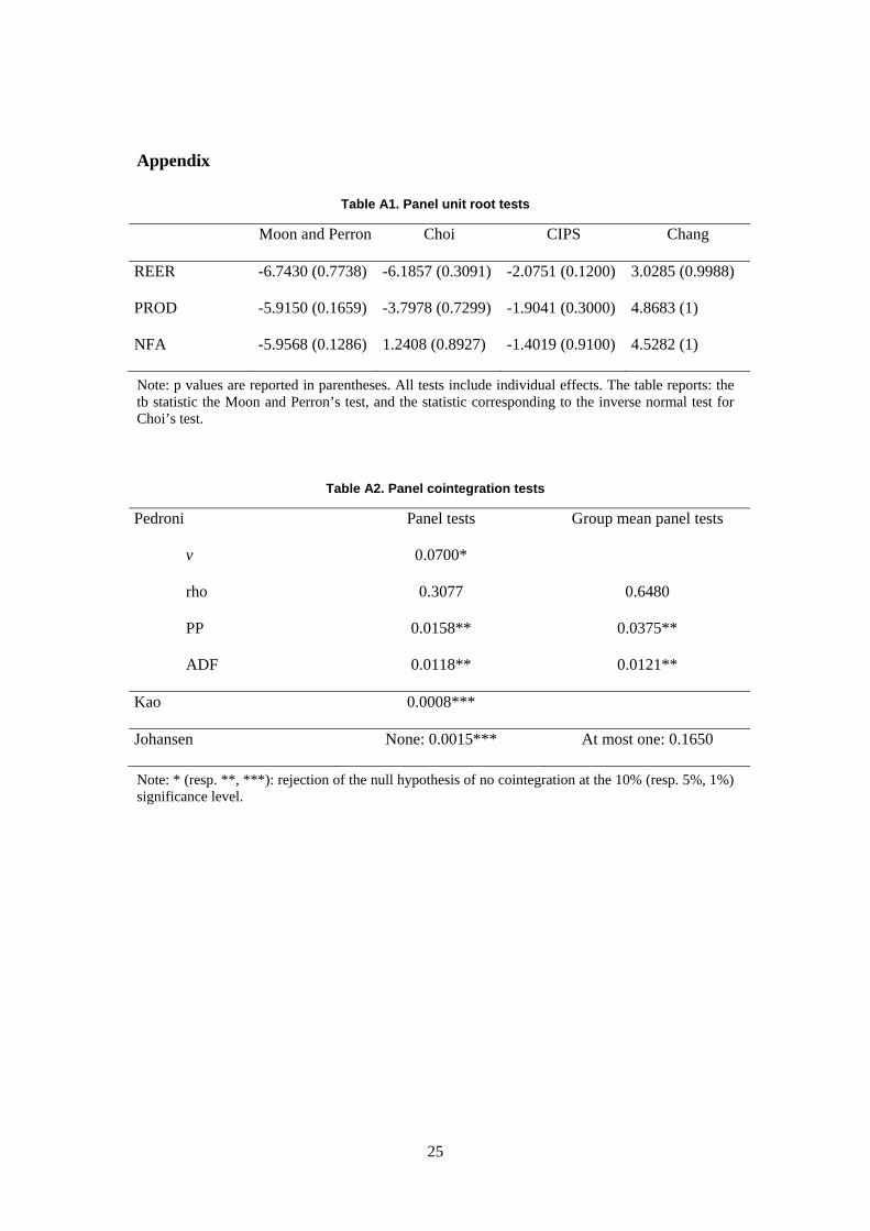
Before estimating Equation (1), panel unit root and cointegration tests have to be applied.

Given that our panel includes countries that are likely to share some common

characteristics, we rely on second-generation panel unit root tests.4 Four tests are considered,

all being based on the unit root null hypothesis. The Moon and Perron (2004) test consists in

testing the unit root hypothesis on de-factored observations, obtained as deviations from the

common components that have been eliminated from the series. The Choi (2002) test also

tests the unit root hypothesis using the modified observed series that allows for the

elimination of the cross-sectional correlations and the potential deterministic trend. More

specifically, it relies on an error-components panel model and removes the cross-section

dependence by eliminating (i) individual effects using the Elliott et al. (1996) methodology

(ERS), and (ii) the time trend effect by centering on the individual mean. The Pesaran

(2007) CIPS test is based on Dickey-Fuller-type regressions augmented with the cross-

section averages of lagged levels and first differences of the individual series. Finally, the

approach suggested by Chang (2002) consists in using the instrumental variable method to

solve the nuisance parameter problem due to cross-sectional dependency: in a first step, for

each cross-section unit, the autoregressive coefficient from an usual ADF regression is

estimated using the instruments generated by an integrable transformation of the lagged

values of the endogenous variable, and, in a second step, a cross-sectional average of the

4 Correlations across individuals constitute nuisance parameters in the first-generation panel unit root tests that are based on the cross-sectional independency hypothesis. Rather than considering correlations across units as nuisance parameters, the category of second-generation tests aims at exploiting these co-movements in order to define new test statistics.

9

individual unit test statistics is considered. As shown in Table A1 in Appendix, all tests

conclude in favour of the null hypothesis, meaning that our three considered series are I(1).

Turning to panel cointegration tests, we rely on Pedroni and Kao tests which are based on

Engle-Granger (1987) two-step (residual-based) cointegration tests. Among the seven tests

proposed by Pedroni (1999, 2004), four of them are based on the within dimension (panel

cointegration tests) and three on the between dimension (group mean panel cointegration

tests). Group mean panel cointegration statistics are more general in the sense that they

allow for heterogeneous coefficients under the alternative hypothesis of cointegration. The

Kao (1999)’s test is close to Pedroni’s tests, but specifies cross-section specific intercepts

and assumes that the coefficients on the first-stage regressors are homogeneous across

individuals. Finally, following the approach suggested by Maddala and Wu (1999), we test

for cointegration by combining Johansen tests from individual cross-sections. Results in

Table A2 in Appendix are globally in favor of the existence of a cointegrating relationship.

Indeed, the null hypothesis of no cointegration between the three considered variables is

rejected according to five Pedroni’s tests. This result is confirmed by Kao and Johansen

tests, which also reject the null hypothesis of no cointegration. Based on these results, it is

now possible to estimate the long-term, cointegrating relationship (1) and to derive the

corresponding misalignments.

Since OLS estimates are biased and dependent on nuisance parameters, we use the Dynamic

OLS (DOLS) method introduced by Kao and Chiang (2000) and Mark and Sul (2003) in the

context of panel cointegration. Roughly speaking, the DOLS procedure consists in

augmenting the cointegrating relationship with lead and lagged differences of the regressors

to control for the endogenous feedback effect. The estimated coefficients are the following:

2314.0ˆ ;2475.0ˆ21 (2)

and the intercept is calculated so that each country has a real effective exchange rate in

equilibrium on average over the period. Both coefficients 1 and 2 are correctly signed: a

1% rise in the relative productivity (resp. in the net foreign asset position) leads to a 0.25%

(resp. 0.23%) real exchange rate appreciation.5

5 As robustness checks, to avoid any bias linked to the current crisis, Equation (1) has been estimated on the shorter 1980-2007 pre-crisis period. Our results are robust since the estimated coefficients are very close to those reported here (the complete results are available upon request to the authors).

10

3.3. Testing for a break in the relation of real exchange rates to their fundamentals

The former results, the existence of the cointegration relation as well as the signs of the

coefficients, show that we retrieve the same results for the euro area as those found in the

previous literature for larger panels (Bénassy-Quéré et al., 2010). Hence, despite the

specificity of the currency union, the real exchange rates are driven in the long run by

exactly the same fundamentals in the euro area as in the rest of the world.

To be sure that some structural break has not occurred after the launch of the euro, we

further verify the stability of this cointegration relationship. To account for possible breaks,

we apply the cointegration tests developed by Westerlund and Edgerton (2007). The tests

are based on the null hypothesis of no cointegration and are robust to both cross-sectional

dependence and unknown heterogeneous breaks in the intercept and/or the slope of the

cointegrating regression. Results show that the null is always rejected, confirming that the

cointegrating relationship is robust to potential level and regime shifts.6

On the whole, the currency union has not changed the long-run relation of real exchange

rates to their fundamentals. The stability of the relation does not preclude that the time for

real exchange rates to adjust to their fundamentals has not lengthened since monetary union.

Indeed, the adjustment delay is likely to have increase because the nominal exchange rate

cannot adjust anymore and prices are rigid in the short-run. The consequence would be

growing currency misalignments within the euro area, as we will see below.

4. EXCHANGE RATE MISALIGNMENTS WITHIN THE EURO AREA

4.1. Characteristics of currency misalignments inside the euro area

We assess the behavioural equilibrium exchange rate (BEER) as the fitted value of Equation

(1) with the estimated coefficients reported in Equations (2):

ititiit NFAPRODBEER 21ˆˆˆ (3)

We then derive the corresponding currency misalignments for each member of the euro

area:

6 Results are available upon request from authors.

11

ititit BEERREERm (4)

A positive misalignment is equivalent to an overvaluation of the currency, while a negative

one is an undervaluation of country’s i currency compared to its fundamentals.

By construction, an increase in overvaluation can stem from the depreciation of the real

equilibrium exchange rate (BEER) or the appreciation in the observed real exchange rate

(REER). This leaves four possible factors for an increase in overvaluation in one country: (i)

a decrease in its relative productivity, that would depreciate its equilibrium exchange rate;

(ii) a decrease in its net foreign assets, generally induced by external deficits, that would

also depreciate the equilibrium exchange rate; and two other factors linked to the

appreciation of its real exchange rate inside the currency union: (iii) a real appreciation of

the euro towards third currencies; (iv) a higher inflation in the home country compared to all

partners. Theoretically, different exposures to trade with third countries is also a factor able

to increase overvaluation in one euro member country without any of the previous factors

involved;7 however, this can be considered as a second-order effect.

Also by construction, the euro effective exchange rate is not directly comparable to the one

of any of the member countries. Indeed it should be more fluctuating because it is calculated

against third currencies with flexible parities, whereas the real effective exchange rates of

member countries are calculated relatively to their trade partners, most of them being inside

the euro area, with completely fixed parities. Hence, the effective exchange rates of euro

area members exhibit smaller fluctuations on average than the euro itself because of the

large weighting to intra-euro zone partners. One the reason underlying monetary union and

previously the European monetary system (EMS) was precisely to stabilize the effective

exchange rates of member countries in order to boost their trade. Consequently, when the

euro plummeted against the dollar and all other key currencies at the very start of monetary

union, there was a drop in the euro real effective parity by 15.7% in 2000 compared to 1998.

Nevertheless, this brought about a much smaller depreciation in the effective exchange rates

of individual euro area countries, the maximum depreciation recorded in any of these

7 Suppose for example that the euro REER is globally stable, but depreciates versus several currencies and appreciates versus the GBP. If one member country trades more with the UK than the whole euro area, its REER will appreciate, everything being equal. This type of effect could affect Ireland whose trade is much more oriented towards the US and the UK than that of the euro area, but is likely to be benign in other member countries.

12

countries being 7.9%. This issue has a direct impact on the misalignments. As the BEER of

the euro area is calculated using the aggregate productivity and foreign asset position of the

euro zone, it is more stable than the observed REER of the euro area. This more stable

equilibrium exchange rate combined with a more variable observed effective parity typically

result in larger misalignments r for the euro than for member countries on average.

4.2. Are currency misalignments homogeneous across euro zone countries?

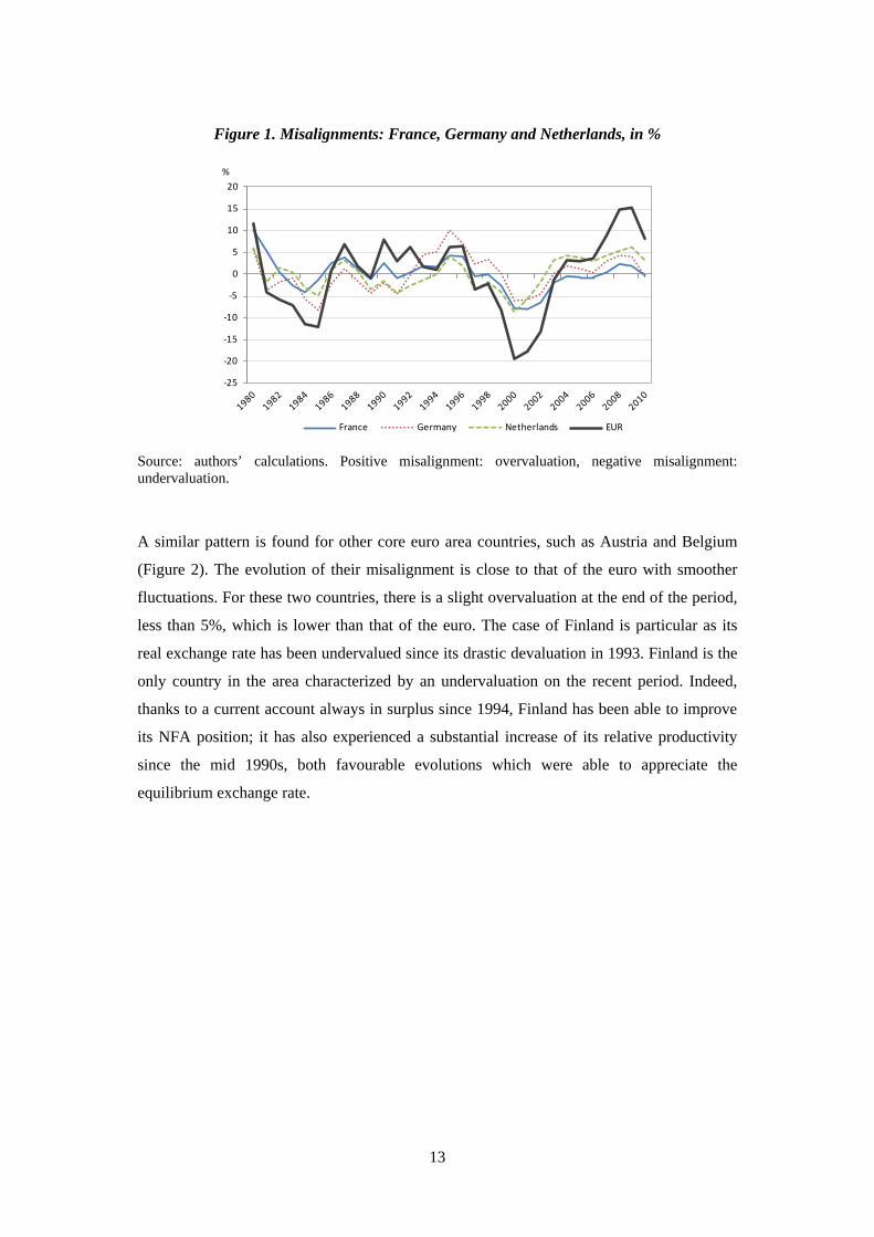
Figures 1 to 3 report the estimated currency misalignment for each euro zone country over

the whole period, together with the euro misalignment. Various interesting facts may be

highlighted from these figures.

Regarding the core countries displayed in Figure 1, the misalignments calculated for France,

Germany and the Netherlands roughly co-move with the euro misalignment though

displaying smoother fluctuations. In the early 2000s, all core countries gained

competitiveness because of the weakness of the euro. Unsurprisingly, the undervaluation of

the member countries was lower than that of the euro for the reasons described in Section

4.1. The phenomenon was reversed at the end of the period, after the euro had strongly

appreciated against third currencies (by 41% from 2000 to 2009 ahead of the 7% drop in

2010). The euro is estimated to be overvalued in 2009 and 2010 (by around 15% and 8%

respectively). The overvaluation is much less pronounced in the individual countries:

Germany and France have real exchange rates nearly at equilibrium in 2010—the reduction

of their overvaluation being mainly due to the depreciation of the euro.

13

Figure 1. Misalignments: France, Germany and Netherlands, in %

‐25

‐20

‐15

‐10

‐5

0

5

10

15

20

France Germany Netherlands EUR

%

Source: authors’ calculations. Positive misalignment: overvaluation, negative misalignment: undervaluation.

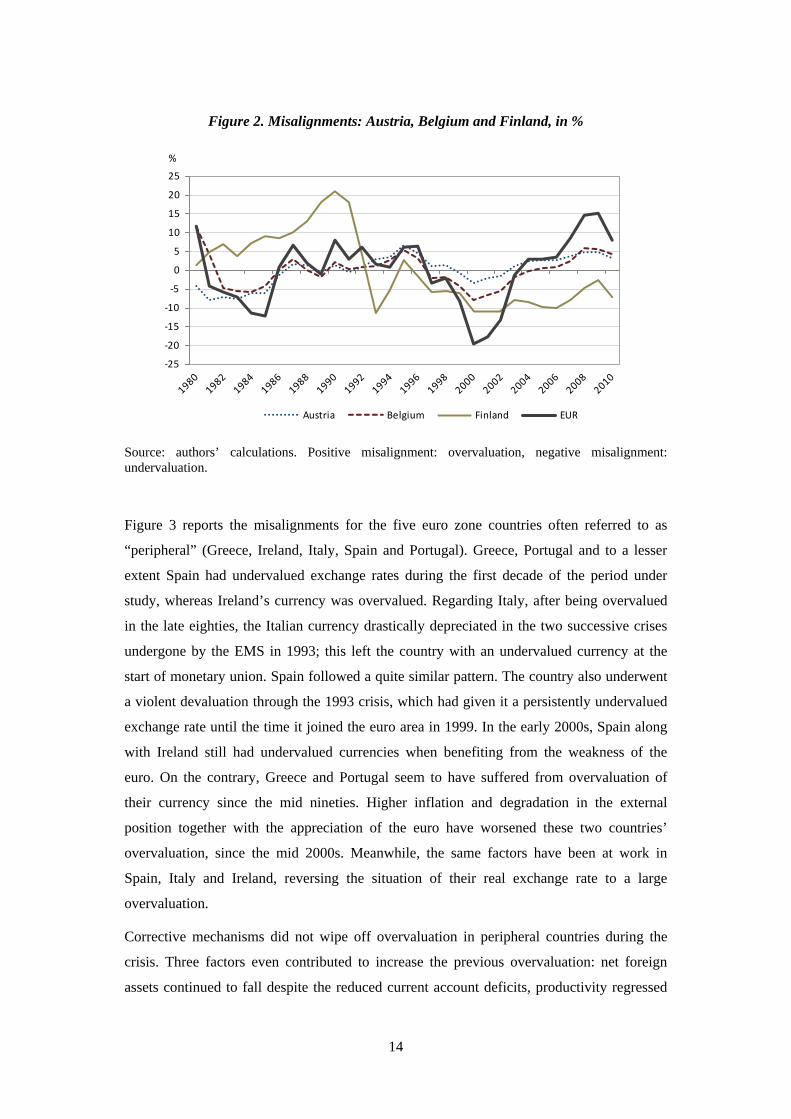
A similar pattern is found for other core euro area countries, such as Austria and Belgium

(Figure 2). The evolution of their misalignment is close to that of the euro with smoother

fluctuations. For these two countries, there is a slight overvaluation at the end of the period,

less than 5%, which is lower than that of the euro. The case of Finland is particular as its

real exchange rate has been undervalued since its drastic devaluation in 1993. Finland is the

only country in the area characterized by an undervaluation on the recent period. Indeed,

thanks to a current account always in surplus since 1994, Finland has been able to improve

its NFA position; it has also experienced a substantial increase of its relative productivity

since the mid 1990s, both favourable evolutions which were able to appreciate the

equilibrium exchange rate.

14

Figure 2. Misalignments: Austria, Belgium and Finland, in %

‐25

‐20

‐15

‐10

‐5

0

5

10

15

20

25

Austria Belgium Finland EUR

%


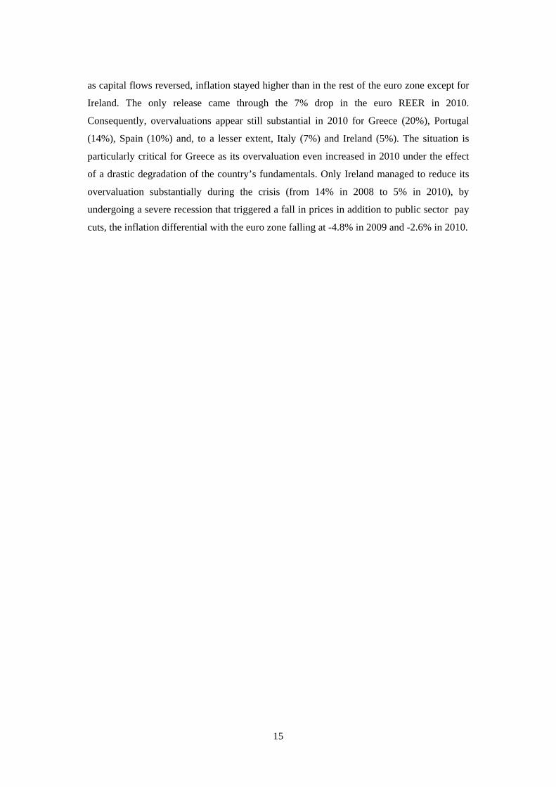
Figure 3 reports the misalignments for the five euro zone countries often referred to as

“peripheral” (Greece, Ireland, Italy, Spain and Portugal). Greece, Portugal and to a lesser

extent Spain had undervalued exchange rates during the first decade of the period under

study, whereas Ireland’s currency was overvalued. Regarding Italy, after being overvalued

in the late eighties, the Italian currency drastically depreciated in the two successive crises

undergone by the EMS in 1993; this left the country with an undervalued currency at the

start of monetary union. Spain followed a quite similar pattern. The country also underwent

a violent devaluation through the 1993 crisis, which had given it a persistently undervalued

exchange rate until the time it joined the euro area in 1999. In the early 2000s, Spain along

with Ireland still had undervalued currencies when benefiting from the weakness of the

euro. On the contrary, Greece and Portugal seem to have suffered from overvaluation of

their currency since the mid nineties. Higher inflation and degradation in the external

position together with the appreciation of the euro have worsened these two countries’

overvaluation, since the mid 2000s. Meanwhile, the same factors have been at work in

Spain, Italy and Ireland, reversing the situation of their real exchange rate to a large

overvaluation.

Corrective mechanisms did not wipe off overvaluation in peripheral countries during the

crisis. Three factors even contributed to increase the previous overvaluation: net foreign

assets continued to fall despite the reduced current account deficits, productivity regressed

15

as capital flows reversed, inflation stayed higher than in the rest of the euro zone except for

Ireland. The only release came through the 7% drop in the euro REER in 2010.

Consequently, overvaluations appear still substantial in 2010 for Greece (20%), Portugal

(14%), Spain (10%) and, to a lesser extent, Italy (7%) and Ireland (5%). The situation is

particularly critical for Greece as its overvaluation even increased in 2010 under the effect

of a drastic degradation of the country’s fundamentals. Only Ireland managed to reduce its

overvaluation substantially during the crisis (from 14% in 2008 to 5% in 2010), by

undergoing a severe recession that triggered a fall in prices in addition to public sector pay

cuts, the inflation differential with the euro zone falling at -4.8% in 2009 and -2.6% in 2010.

16

Figure 3. Misalignments in peripheral countries, in %

‐25

‐20

‐15

‐10

‐5

0

5

10

15

20

25

Greece Portugal Ireland EUR

%

‐25

‐20

‐15

‐10

‐5

0

5

10

15

20

Italy Spain EUR

%


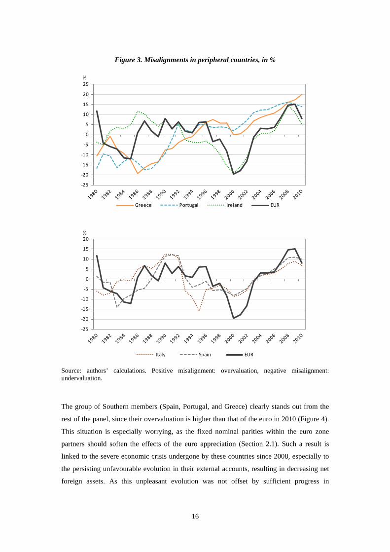
The group of Southern members (Spain, Portugal, and Greece) clearly stands out from the

rest of the panel, since their overvaluation is higher than that of the euro in 2010 (Figure 4).

This situation is especially worrying, as the fixed nominal parities within the euro zone

partners should soften the effects of the euro appreciation (Section 2.1). Such a result is

linked to the severe economic crisis undergone by these countries since 2008, especially to

the persisting unfavourable evolution in their external accounts, resulting in decreasing net

foreign assets. As this unpleasant evolution was not offset by sufficient progress in

17

productivity, the equilibrium exchange rates of these countries have tended to depreciate

since the mid-2000s, especially for Portugal and Spain. As the observed real exchange rates

appreciated due to (i) the euro appreciation and (ii) higher inflation than in the core

countries, this resulted in an ever increasing gap between the appreciating observed parity

and the depreciating equilibrium exchange rate, i.e. in an increasing overvaluation.

Figure 4. Misalignments in euro area countries, in 2010, in %

4.3. Have currency misalignments widened since monetary union?

We now investigate whether the currency misalignments have been reduced or amplified

after the adoption of the single currency. On the one hand, monetary union could have

stabilized the effective parities as the bulk of trade is made with intra-zone partners. On the

other hand, fixed nominal exchange rates could have generated overvaluation in high

inflation countries, especially in Southern Europe.

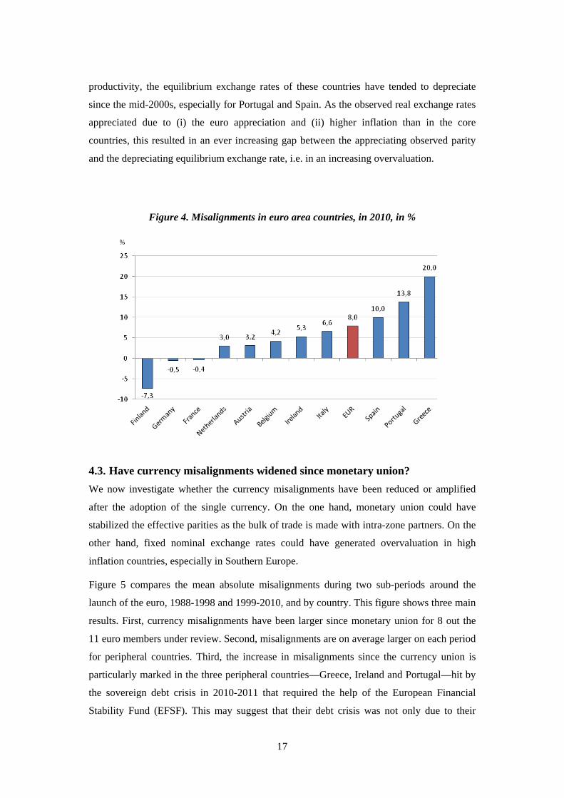
Figure 5 compares the mean absolute misalignments during two sub-periods around the

launch of the euro, 1988-1998 and 1999-2010, and by country. This figure shows three main

results. First, currency misalignments have been larger since monetary union for 8 out the

11 euro members under review. Second, misalignments are on average larger on each period

for peripheral countries. Third, the increase in misalignments since the currency union is

particularly marked in the three peripheral countries—Greece, Ireland and Portugal—hit by

the sovereign debt crisis in 2010-2011 that required the help of the European Financial

Stability Fund (EFSF). This may suggest that their debt crisis was not only due to their

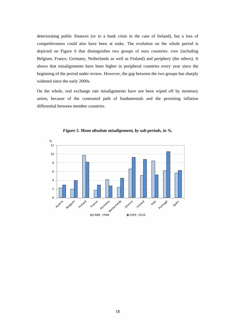
18

deteriorating public finances (or to a bank crisis in the case of Ireland), but a loss of

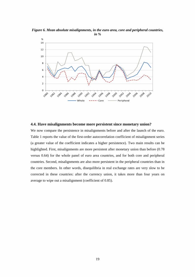
competitiveness could also have been at stake. The evolution on the whole period is

depicted on Figure 6 that distinguishes two groups of euro countries: core (including

Belgium, France, Germany, Netherlands as well as Finland) and periphery (the others). It

shows that misalignments have been higher in peripheral countries every year since the

beginning of the period under review. However, the gap between the two groups has sharply

widened since the early 2000s.

On the whole, real exchange rate misalignments have not been wiped off by monetary

union, because of the contrasted path of fundamentals and the persisting inflation

differential between member countries.

Figure 5. Mean absolute misalignment, by sub-periods, in %.

0

2

4

6

8

10

12

1988 ‐1998 1999 ‐ 2010

%

19

Figure 6. Mean absolute misalignments, in the euro area, core and peripheral countries, in %

0

2

4

6

8

10

12

14

Whole Core Peripheral

%

4.4. Have misalignments become more persistent since monetary union?

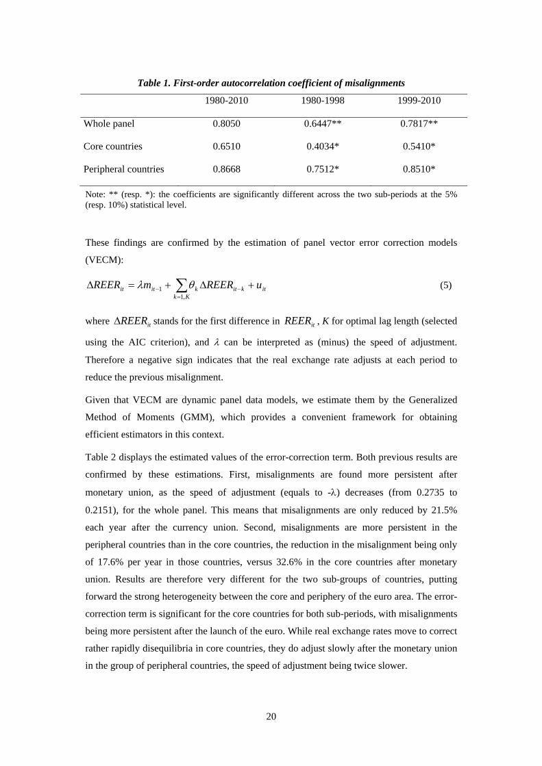
We now compare the persistence in misalignments before and after the launch of the euro.

Table 1 reports the value of the first-order autocorrelation coefficient of misalignment series

(a greater value of the coefficient indicates a higher persistence). Two main results can be

highlighted. First, misalignments are more persistent after monetary union than before (0.78

versus 0.64) for the whole panel of euro area countries, and for both core and peripheral

countries. Second, misalignments are also more persistent in the peripheral countries than in

the core members. In other words, disequilibria in real exchange rates are very slow to be

corrected in these countries: after the currency union, it takes more than four years on

average to wipe out a misalignment (coefficient of 0.85).

20

Table 1. First-order autocorrelation coefficient of misalignments

1980-2010 1980-1998 1999-2010

Whole panel 0.8050 0.6447** 0.7817**

Core countries 0.6510 0.4034* 0.5410*

Peripheral countries 0.8668 0.7512* 0.8510*

Note: ** (resp. *): the coefficients are significantly different across the two sub-periods at the 5% (resp. 10%) statistical level.

These findings are confirmed by the estimation of panel vector error correction models

(VECM):

Kk

itkitkitit uREERmREER,1

1 (5)

where itREER stands for the first difference in itREER , K for optimal lag length (selected

using the AIC criterion), and can be interpreted as (minus) the speed of adjustment.

Therefore a negative sign indicates that the real exchange rate adjusts at each period to

reduce the previous misalignment.

Given that VECM are dynamic panel data models, we estimate them by the Generalized

Method of Moments (GMM), which provides a convenient framework for obtaining

efficient estimators in this context.

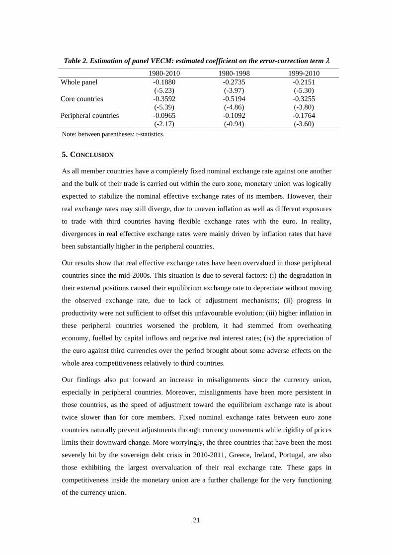
Table 2 displays the estimated values of the error-correction term. Both previous results are

confirmed by these estimations. First, misalignments are found more persistent after

monetary union, as the speed of adjustment (equals to -) decreases (from 0.2735 to

0.2151), for the whole panel. This means that misalignments are only reduced by 21.5%

each year after the currency union. Second, misalignments are more persistent in the

peripheral countries than in the core countries, the reduction in the misalignment being only

of 17.6% per year in those countries, versus 32.6% in the core countries after monetary

union. Results are therefore very different for the two sub-groups of countries, putting

forward the strong heterogeneity between the core and periphery of the euro area. The error-

correction term is significant for the core countries for both sub-periods, with misalignments

being more persistent after the launch of the euro. While real exchange rates move to correct

rather rapidly disequilibria in core countries, they do adjust slowly after the monetary union

in the group of peripheral countries, the speed of adjustment being twice slower.

21

Table 2. Estimation of panel VECM: estimated coefficient on the error-correction term

1980-2010 1980-1998 1999-2010 Whole panel -0.1880

(-5.23) -0.2735 (-3.97)

-0.2151 (-5.30)

Core countries -0.3592 (-5.39)

-0.5194 (-4.86)

-0.3255 (-3.80)

Peripheral countries -0.0965 (-2.17)

-0.1092 (-0.94)

-0.1764 (-3.60)

Note: between parentheses: t-statistics.

5. CONCLUSION

As all member countries have a completely fixed nominal exchange rate against one another

and the bulk of their trade is carried out within the euro zone, monetary union was logically

expected to stabilize the nominal effective exchange rates of its members. However, their

real exchange rates may still diverge, due to uneven inflation as well as different exposures

to trade with third countries having flexible exchange rates with the euro. In reality,

divergences in real effective exchange rates were mainly driven by inflation rates that have

been substantially higher in the peripheral countries.

Our results show that real effective exchange rates have been overvalued in those peripheral

countries since the mid-2000s. This situation is due to several factors: (i) the degradation in

their external positions caused their equilibrium exchange rate to depreciate without moving

the observed exchange rate, due to lack of adjustment mechanisms; (ii) progress in

productivity were not sufficient to offset this unfavourable evolution; (iii) higher inflation in

these peripheral countries worsened the problem, it had stemmed from overheating

economy, fuelled by capital inflows and negative real interest rates; (iv) the appreciation of

the euro against third currencies over the period brought about some adverse effects on the

whole area competitiveness relatively to third countries.

Our findings also put forward an increase in misalignments since the currency union,

especially in peripheral countries. Moreover, misalignments have been more persistent in

those countries, as the speed of adjustment toward the equilibrium exchange rate is about

twice slower than for core members. Fixed nominal exchange rates between euro zone

countries naturally prevent adjustments through currency movements while rigidity of prices

limits their downward change. More worryingly, the three countries that have been the most

severely hit by the sovereign debt crisis in 2010-2011, Greece, Ireland, Portugal, are also

those exhibiting the largest overvaluation of their real exchange rate. These gaps in

competitiveness inside the monetary union are a further challenge for the very functioning

of the currency union.

22

References

Alberola, E. (2003), “Misalignment, liabilities dollarization and exchange rate adjustment in Latin America”, Banco de España documento de trabajo n°0309, Banco de España, Madrid.

Alberola, E., Cervero, S.G., Lopez, H. and A. Ubide (1999), “Global equilibrium exchange rates: Euro, Dollar, ‘ins’, ‘outs’ and other major currencies in a panel cointegration framework”, IMF Working Paper WP/99/175, International Monetary Fund, Washington DC.

Alberola, E., Cervero, S.G., Lopez, H. and A. Ubide (2002), “Quo vadis euro?”, The European Journal of Finance, 8(4), 346–351.

Andersson, M., Masuch, K. and M. Schiffbauer (2009), “Determinants of inflation and price level differentials across the euro area countries”, ECB Working Paper n°1129, European Central Bank, Frankfurt, December.

Barnes, S., Lawson, J. and A. Radziwill (2010), “Current account imbalances in the euro area: a comparative perspective”, OECD Economics Department Working Paper n°826, Organisation for Economic Co-operation and Development, Paris.

Barrios, S., Deroose, S., Langedijk, S. and L. Pench (2010), “External Imbalances and Public Finances in the EU”, Occasional Papers n°66, European Commission, Economic and Financial Affairs, Brussels.

Beck, G.W., Hubrich, K. and M. Marcellino (2009), “Regional inflation dynamics within and across euro area countries and a comparison with the United States”, Economic Policy, 24(57), 141–184.

Bénassy-Quéré, A., Béreau, S. and V. Mignon (2009), “Robust estimations of equilibrium exchange rates within the G20: A panel BEER approach”, Scottish Journal of Political Economy, 56(5), 608-633.

Bénassy-Quéré, A., Béreau, S. and V. Mignon (2010), “On the complementarity of equilibrium exchange-rate approaches”, Review of International Economics, 18(4), 618-632.

Berger, H. and V. Nitsch (2010), “The Euro’s Effect on Trade Imbalances”, IMF Working Paper WP/10/226, International Monetary Fund, Washington DC.

Blanchard, O. and F. Giavazzi (2002), “Current Account Deficits in the Euro Area. The End of the Feldstein Horioka Puzzle?”, Brookings Papers on Economic Activity, 2.

Boone, P. and S. Johnson (2011), “Europe on the Brink”, Policy Brief n°11-13, Peterson Institute for International Economics, Washington D.C., July.

Bulır, A. and J. Hurnık (2008), “Why has inflation in the European Union stopped converging?”, Journal of Policy Modeling, 30, 341–347.

Bussière, M., Chudik, A. and A. Mehl (2011), “Does the Euro Make a Difference? Spatio-Temporal transmission of Global Shocks to Real Effective Exchange Rates in an Infinite VAR”, ECB Working Paper n°1292, European Central Bank, Frankfurt, February.

Chang, Y. (2002), “Nonlinear IV Unit Root Tests in Panels with Cross-Sectional Dependency”, Journal of Econometrics, 110, 261-292.

23

Chinn, M. and E. Prasad (2003), “Medium Term Determinants of Current Accounts in Industrial and Developing Countries: An Empirical Exploration”, Journal of International Economics, 59(1), 47-76.

Choi, I. (2002), “Combination unit root tests for cross-sectionally correlated panels”, Mimeo, Hong Kong University of Science and Technology.

Clark, P.B. and R. MacDonald (1998), “Exchange Rates and Economic Fundamentals - A Methodological Comparison of BEERs and FEERs”, IMF Working Papers WP/98/67, International Monetary Fund, Washington DC.

Cline, W. and J. Williamson (2011), “The current currency situation”, Policy Brief n°PB11-18, Petersen Institute for International Economics, Washington, DC.

Corsetti, G. (2010), “The ‘original sin’ in the Eurozone”, VoxEU.org, 9, May.

Corsetti, G. and H. Pesaran (2012), “Beyond fiscal federalism: what does it take to save the euro?”, VoxEU.org, 9, January.

De Grauwe, P. (2011), “Governance of a Fragile Eurozone”, CEPS Working Document n°346, Centre for European Policy Studies, Brussels, May.

Deustche Bank (2010), “On the problems of macroeconomic imbalances in the euro area”, Monthly bulletin, July.

Elliott, G., Rothenberg, T.J. and J.H. Stock (1996), “Efficient tests for an autoregressive unit root”, Econometrica, 64, 813-836.

Engel, C. (1995), “Accounting for U.S. real exchange rate changes”, NBER Working Paper n°5394, National Bureau of Economic Research, Cambridge, Massachusetts.

Engle, R.F. and C.W.J. Granger (1987), “Co-integration and Error Correction: Representation, Estimation, and Testing”, Econometrica, 55(2), 251-276.

Frankel, J. A. and A. K. Rose (1998), “The endogeneity of the optimum currency area criteria”, Economic Journal, 108, 1009–1025.

Giavazzi, F. and L. Spaventa (2010), “Why the Current Account Matters in a Monetary Union: Lessons from the Financial Crisis in the Euro Area”, CEPR Discussion Paper n°8008, Centre for Economic Policy Research, London, September.

Gros, D. (2011a), “External versus Domestic Debt in the Euro Crisis”, CEPS Policy Brief n°234, Centre for European Policy Studies, Brussels, May.

Gros, D. (2011b), “Speculative Attacks within or outside a Monetary Union: Default versus Inflation (what to do today)”, CEPS Policy Brief n°257, Centre for European Policy Studies, Brussels, November.

Higgins, M. and T. Klitgaard (2011), “Saving Imbalances and the Euro Area Sovereign Debt Crisis”, Current Issues in Economics and Finance, 17(5), Federal Reserve Bank of New York.

Honohan, P. and P.R. Lane (2003), “Divergent inflation rates in EMU”, Economic Policy, 18(37), 357-394.

Jaumotte, F. and P. Sodsriwiboon (2010), “Current Account Imbalances in the Southern Euro Area”, IMF Working Paper WP/10/139, International Monetary Fund, Washington DC.

Jeong, S., Mazier, J. and J. Saadoui (2010), “Exchange Rate Misalignments at World and European Levels: A FEER Approach”, CEPN Working Papers No. 2010-03, University of Paris Nord, France.

24

Kao, C. (1999), “Spurious regression and residual-based tests for cointegration in panel data”, Journal of Econometrics, 90, 1-44.

Kao, C. and M.H. Chiang (2000), “On the estimation and inference of a cointegrated regression in panel data”, in B. Baltagi and C. Kao, eds, Advances in Econometrics, 15, 179-222, Elsevier Science.

Klau, M. and S.S. Fung (2006), “The new BIS effective exchange rate indices”, BIS Quarterly Review, 51-65.

Lane, P. (2010), “International Financial Integration and the External Positions of Euro Area Member Countries”, OECD Economics Department Working Papers n°830, Organisation for Economic Co-operation and Development, Paris.

Lane, P. and G. Milesi-Ferretti, (2007), "The external wealth of nations mark II: Revised and extended estimates of foreign assets and liabilities, 1970–2004", Journal of International Economics, 73, 223-250. http://www.philiplane.org/EWN.html.

Maddala, G. and S. Wu (1999), “A comparative study of unit root tests and a new simple test”, Oxford Bulletin of Economics and Statistics, 61, 631-652.

Mark, N. and D. Sul (2003), “Cointegration vector estimation by panel Dynamic OLS and long-run money demand”, Oxford Bulletin of Economics and Statistics, 65, 655-680.

Mongelli, F. and C. Wyplosz (2008), “The euro at ten: unfulfilled and unexpected challenges”, Fifth ECB Central Banking Conference, 13 and 14 November.

Moon, H.R. and B. Perron (2004), “Testing for a unit root in panels with dynamic factors”, Journal of Econometrics, 122, 81-126.

Mundell, R.A. (1961), “A Theory of Optimum Currency Areas”, American Economic Review, 51, 657-665.

Pedroni, P. (1999), “Critical values for cointegration tests in heterogeneous panels with multiple regressors”, Oxford Bulletin of Economics and Statistics, S1, 61, 653-670.

Pedroni, P. (2004), “Panel cointegration. Asymptotic and finite sample properties of pooled time series tests with an application to the PPP hypothesis”, Econometric Theory, 20, 597-625.

Pesaran, M.H. (2007), “A simple panel unit root test in the presence of cross-section dependence”, Journal of Econometrics, 22, 265-312.

Pisani-Ferry, J. (2012), “The euro crisis and the new impossible trinity”, Bruegel policy Contribution, Issue 2012/01, Bruegel, Brussels, January. http://www.bruegel.org/publications/publication-detail/publication/674-the-euro-crisis-and-the-new-impossible-trinity/

Rabanal, P. (2009), “Inflation differentials between Spain and the EMU: A DSGE perspective”, Journal of Money, Credit, and Banking, 41(6), 1142–1166.

Rose, A.K., and C. Engel (2000), “Currency Unions and International Integration”, NBER Working Papers n°7872, National Bureau of Economic Research, Cambridge, Massachusetts.

Schmitz, B. and J. von Hagen (2009), “Current Account Imbalances and Financial Integration in the Euro Area”, CEPR Discussion Papers n°7262, Centre for Economic Policy Research, London.

Westerlund, J. and D. Edgerton (2007), “Simple tests for cointegration in dependent panels with structural breaks”, Oxford Bulletin of Economics and Statistics, 70, 665-704.

25

Appendix

Table A1. Panel unit root tests

Moon and Perron Choi CIPS Chang

REER -6.7430 (0.7738) -6.1857 (0.3091) -2.0751 (0.1200) 3.0285 (0.9988)

PROD -5.9150 (0.1659) -3.7978 (0.7299) -1.9041 (0.3000) 4.8683 (1)

NFA -5.9568 (0.1286) 1.2408 (0.8927) -1.4019 (0.9100) 4.5282 (1)

Note: p values are reported in parentheses. All tests include individual effects. The table reports: the tb statistic the Moon and Perron’s test, and the statistic corresponding to the inverse normal test for Choi’s test.

Table A2. Panel cointegration tests

Pedroni Panel tests Group mean panel tests

v 0.0700*

rho 0.3077 0.6480

PP 0.0158** 0.0375**

ADF 0.0118** 0.0121**

Kao 0.0008***

Johansen None: 0.0015*** At most one: 0.1650

Note: * (resp. **, ***): rejection of the null hypothesis of no cointegration at the 10% (resp. 5%, 1%) significance level.

On currency misalignments within the euro area

Documents

Transcript of On currency misalignments within the euro area