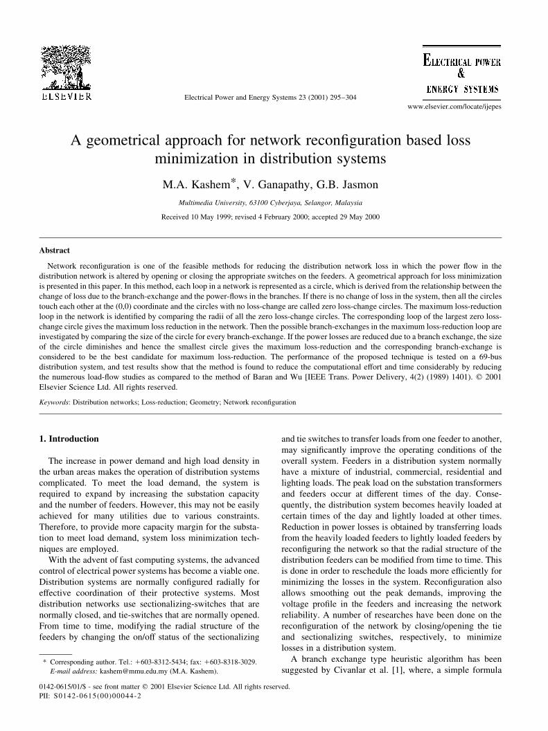
A geometrical approach for network recon®guration based lossminimization in distribution systems

M.A. Kashem*, V. Ganapathy, G.B. Jasmon

Multimedia University, 63100 Cyberjaya, Selangor, Malaysia

Received 10 May 1999; revised 4 February 2000; accepted 29 May 2000

Abstract

Network recon®guration is one of the feasible methods for reducing the distribution network loss in which the power ¯ow in the

distribution network is altered by opening or closing the appropriate switches on the feeders. A geometrical approach for loss minimization

is presented in this paper. In this method, each loop in a network is represented as a circle, which is derived from the relationship between the

change of loss due to the branch-exchange and the power-¯ows in the branches. If there is no change of loss in the system, then all the circles

touch each other at the (0,0) coordinate and the circles with no loss-change are called zero loss-change circles. The maximum loss-reduction

loop in the network is identi®ed by comparing the radii of all the zero loss-change circles. The corresponding loop of the largest zero loss-

change circle gives the maximum loss reduction in the network. Then the possible branch-exchanges in the maximum loss-reduction loop are

investigated by comparing the size of the circle for every branch-exchange. If the power losses are reduced due to a branch exchange, the size

of the circle diminishes and hence the smallest circle gives the maximum loss-reduction and the corresponding branch-exchange is

considered to be the best candidate for maximum loss-reduction. The performance of the proposed technique is tested on a 69-bus

distribution system, and test results show that the method is found to reduce the computational effort and time considerably by reducing

the numerous load-¯ow studies as compared to the method of Baran and Wu [IEEE Trans. Power Delivery, 4(2) (1989) 1401). q 2001

Elsevier Science Ltd. All rights reserved.

Keywords: Distribution networks; Loss-reduction; Geometry; Network recon®guration

1. Introduction

The increase in power demand and high load density in

the urban areas makes the operation of distribution systems

complicated. To meet the load demand, the system is

required to expand by increasing the substation capacity

and the number of feeders. However, this may not be easily

achieved for many utilities due to various constraints.

Therefore, to provide more capacity margin for the substa-

tion to meet load demand, system loss minimization tech-

niques are employed.

With the advent of fast computing systems, the advanced

control of electrical power systems has become a viable one.

Distribution systems are normally con®gured radially for

effective coordination of their protective systems. Most

distribution networks use sectionalizing-switches that are

normally closed, and tie-switches that are normally opened.

From time to time, modifying the radial structure of the

feeders by changing the on/off status of the sectionalizing

and tie switches to transfer loads from one feeder to another,

may signi®cantly improve the operating conditions of the

overall system. Feeders in a distribution system normally

have a mixture of industrial, commercial, residential and

lighting loads. The peak load on the substation transformers

and feeders occur at different times of the day. Conse-

quently, the distribution system becomes heavily loaded at

certain times of the day and lightly loaded at other times.

Reduction in power losses is obtained by transferring loads

from the heavily loaded feeders to lightly loaded feeders by

recon®guring the network so that the radial structure of the

distribution feeders can be modi®ed from time to time. This

is done in order to reschedule the loads more ef®ciently for

minimizing the losses in the system. Recon®guration also

allows smoothing out the peak demands, improving the

voltage pro®le in the feeders and increasing the network

reliability. A number of researches have been done on the

recon®guration of the network by closing/opening the tie

and sectionalizing switches, respectively, to minimize

losses in a distribution system.

A branch exchange type heuristic algorithm has been

suggested by Civanlar et al. [1], where, a simple formula

Electrical Power and Energy Systems 23 (2001) 295±304

0142-0615/01/$ - see front matter q 2001 Elsevier Science Ltd. All rights reserved.

PII: S0142-0615(00)00044-2

www.elsevier.com/locate/ijepes

* Corresponding author. Tel.: 1603-8312-5434; fax: 1603-8318-3029.

E-mail address: kashem@mmu.edu.my (M.A. Kashem).

has been developed for determination of change in power

loss due to a branch exchange. A different method has been

proposed by Baran and Wu [2] to identify the branches to be

exchanged using heuristic approach to minimize the search

for selecting the switching options. Merlin and Back [3]

have used the branch and bound type optimization technique

to ®nd the minimum loss con®guration. Following the

method of Ref. [3], Shirmohammdi and Hong [4] have

developed a heuristic algorithm. In their method, the solu-

tion is obtained by ®rst closing all the switches, which are

then opened one after another so as to establish the optimum

¯ow pattern in the network. Goswami and Basu [5] also

have proposed a heuristic algorithm for feeder recon®gura-

tion by solving the KVL and KCL equations for the network

with line impedances replaced by their corresponding resis-

tances only. Also, instead of closing all the switches to form

a meshed network and opening the switches one after

another, the authors of Ref. [5] adapted the method of clos-

ing one switch at a time and back to the radial con®guration

by opening the same, or a different switch of the loop,

depending upon the result of the optimal ¯ow pattern

through the switches of the same loop. Broadwater et al.

[6] have applied the Civanlar's method [1] and Huddle-

ston's quadratic loss function and multiple switching pair

operation method [7] to solve the minimum loss recon®-

guration problem. Peponis et al. [8] have used the switch-

exchange and sequential switch opening methods for

recon®guration of the network for loss reduction. The meth-

ods proposed by Rubin Taleski et al. [9] and Kashem et al.

[10] are based on branch-exchange technique for recon®-

guration to minimize distribution losses. Methods in Refs.

[11,12] have been suggested to implement on-line control

strategies for power system planing and operations based on

continuous network recon®guration for loss minimization.

In this paper, a geometrical method for the network

recon®guration based loss minimization problem is devel-

oped and presented. The ®rst stage of the method determines

the maximum loss-reduction loop by comparing the size of

the circle for every loop. In a distribution system, a loop is

associated by a tie-line and hence there are several loops in

the system. To obtain the maximum loss-reduction loop, the

size of the modi®ed zero loss-change circles are compared,

and the loop with the largest circle is identi®ed for maximum

loss-reduction. The second stage determines the switching-

operation to be executed in that loop to reach a minimum loss

network con®guration by comparing the size of the loop

circle for each branch-exchange. The smallest circle is iden-

ti®ed for the best solution, as the size of the loop circle is

reduced when the losses are minimized. By utilizing this

proposed method, an optimal or near optimal con®guration

for loss reduction can be obtained with reduced computa-

tional effort because it does not have to check the branches

in all the loops to obtain maximum loss-reduction as used in

Ref. [2]. The proposed geometrical method will be a useful

tool for distribution engineers to quickly solve the problem in

network recon®guration for loss minimization.

2. Formulation of the loss reduction problem

Feeder recon®guration is performed by changing the

open/close status of the sectionalizing and tie switches.

Distribution systems are normally con®gured radially. The

system is recon®gured for many purposes. In system recon-

®guration, a whole feeder or part of a feeder is transferred to

another feeder by closing a tie switch connecting the two

while an appropriate sectionalizing switch must be opened

to preserve the radial structure. The loss minimization

problem addressed in this paper determines the open/close

states of the tie and sectionalizing switches in order to achieve

a maximum reduction in power losses. The change in losses

can be easily estimated from the two power ¯ow solutions,

before and after feeder recon®guration. However, the number

of switching options even for a moderate size distribution

system is so large that a large number of load ¯ow solutions

have to be executed for all the possible options. It becomes not

only inef®cient from a computational point of view, but also

unrealistic as a feeder recon®guration strategy. Therefore, it is

desirable to propose a method that can provide a criterion that

may be used to eliminate undesirable switching options.

3. Proposed geometrical method for power lossreduction

A radial distribution network can be represented by

several loops. The number of loops is equal to the number

of tie-lines because one tie-line can only make one loop

when it is connected. The proposed method will estimate

the loss reduction of a network from a switching operation

by considering several loops in a distribution system. A loop

in a radial network is created with reference to a tie-line t as

shown in Fig. 1. There is a voltage difference across the

normally open tie switch in the tie-line. The higher voltage

drop side of the tie switch is called the lower voltage side

(lv-side) and the lower voltage drop side of the tie switch is

called higher voltage side (hv-side) of the loop. The lower

M.A. Kashem et al. / Electrical Power and Energy Systems 23 (2001) 295±304296

Fig. 1. A typical loop

voltage and higher voltage-sides in the ®gure are denoted by

l and h, respectively.

Consider the branch exchange between branches t and m

where t is the open branch and m is the closed branch in Fig.

1. The loop is divided into two parts by the open branch t in

which the ®rst part consisting the branches in the loop that

extends between nodes 0 to l and the second part consisting

the branches that extends between nodes 0 to h. The loss

reduction formula due to this branch exchange as given in

Ref. [2] is rewritten as follows:

DLPtm � 2Pm

XrlPl 2

XrhPh

� �1 2Qm

XrlQl 2

XrhQh

� �2 P2

m 1 Q2m

� �rloop

�1�where DLPtm is the incremental power loss reduction due to

branch exchange t±m, Pm the real power ¯ow in branch m

(to be removed), Qm the reactive power ¯ow in branch m (to

be removed), rlPl the product of rP on the lv-side of the loop,

rhPh the product of rP on the hv-side of the loop and rloop the

total branch resistance around the loop at which the branch-

¯ows exist. If DLPtm . 0; loss reduction is positive and

hence losses are reduced, and if DLPtm , 0; loss reduction

is negative and hence losses are increased.

Eq. (1) can be rearranged as shown below to be repre-

sented by a circle:

Pm 2A

C

� �2

1 Qm 2B

C

� �2

� A2 1 B2

C22

DLPtm

C�2�

where A � PrlPl 2

PrhPh; B � P

rlQl 2P

rhQh and

C � rloop.

This is called the loop circle. The center of the loop circle

is �A=C; B=C� and its radius is

A2 1 B2

C22

DLPtm

C

" #1=2

The zero loss change loop circle is the one which gives the

change in loss to be zero (i.e.DLPtm � 0). It can be repre-

sented as follows:

Pm 2A

C

� �2

1 Qm 2B

C

� �2

� A2 1 B2

C2�3�

Hence the radius of the loop circle is ��A2 1 B2�=�C2��1=2 for

zero loss change (i.e. DLPtm � 0) and is decreased if loss-

reduction occurs in the loop.

Again, Eq. (1) can be rearranged by separating the lv and

hv-sides and using the fact that rloop � rl 1 rh. Eq. (1)

becomes

DLPtm � DLPl 1 DLPh

�"

2Pm

XrlPl

!1 2Qm

XrlQl

!2

P2

m 1 Q2m

!Xrl

#

1

"22Pm

XrhPh

!22Qm

XrhQh

!2

P2

m1 Q2m

!Xrh

#�4a�

where

DLPl � 2Pm

XrlPl

� �1 2Qm

XrlQl

� �2 P2

m 1 Q2m

� �Xrl

�4b�DLPh � 22Pm

XrhPh

� �22Qm

XrhQh

� �2 P2

m 1 Q2m

� �Xrh �4c�

DLPl is the loss reduction for the lv-side, DLPh the loss

reduction for hv-side and rl and rh the resistances at lv and

hv-sides, respectively.

Eqs. (4b) and (4c) can also be rearranged to represent

circle-equations as

lv-side circle:

Pm 2X

rlPl

� ��Xrl

� �2

1 Qm 2X

rlQl

� ��Xrl

� �2

�X

rlPl

� ��Xrl

� �2

1X

rlQl

� ��Xrl

� �2

2DLPl=X

rl

�5a�

hv-side circle:

Pm 1X

rhPh

� ��Xrh

� �2

1 Qm 1X

rhQh

� ��Xrh

� �2

�X

rhPh

� ��Xrh

� �2

1X

rhQh

� ��Xrh

� �2

2DLPh=X

rh (5b)

If the loss-change is zero due to the branch-exchange,

then DLPtm � 0. One of the typical cases is DLP1 � 0 and

DLPh � 0. The equations (5a) and (5b) will now become

Zero loss-change lv-side circle:

Pm 2X

rlPl

� ��Xrl

� �2

1 Qm 2X

rlQl

� ��Xrl

� �2

�X

rlPl

� ��Xrl

� �2

1X

rlQl

� ��Xrl

� �2

(6a)

Zero loss-change hv-side circle:

Pm 1X

rhPh

� ��Xrh

� �2

1 Qm 1X

rhQh

� ��Xrh

� �2

�X

rhPh

� ��Xrh

� �2

1X

rhQh

� ��Xrh

� �2

�6b�

The proposed geometrical method is developed based on the

formation of circles from Eqs. (1)±(6). The equations are

represented by a set of circles. The lv-side and hv-side

M.A. Kashem et al. / Electrical Power and Energy Systems 23 (2001) 295±304 297

circles are drawn from the relationship between the loss

reduction (DLPl, DLPh) and the power transfer (Pm, Qm).

The loop circle is the resultant of the two circles which

can also be drawn by using Equation (2). For the above

typical case where DLPtm � 0, DLPl � 0 and DLPh � 0,

all the circles touch each other at the (0,0) coordinate as

shown in Fig. 2. These circles are called zero loss-change

circles.

It is proven that if the values of the termsP

rlPl andPrlQl are greater than the values of the terms

PrhPh andP

rhQh; respectively, then the loop circle will be in lv-side

circle as shown in Fig. 2(a). In this case, positive loss-reduc-

tion is obtained and losses will be reduced for a switching

operation in the loop. On the other hand, if the values of the

termsP

rlPl andP

rlQl are smaller than the values of the

termsP

rhPh andP

rhQh; respectively, then the loss reduc-

tion value, DLPtm in Eq. (1) will be negative and hence the

loop circle will be in hv-side circle as shown in Fig. 2(b).

For this case, losses will not be reduced for any switching

operation in the loop because of negative loss-reduction.

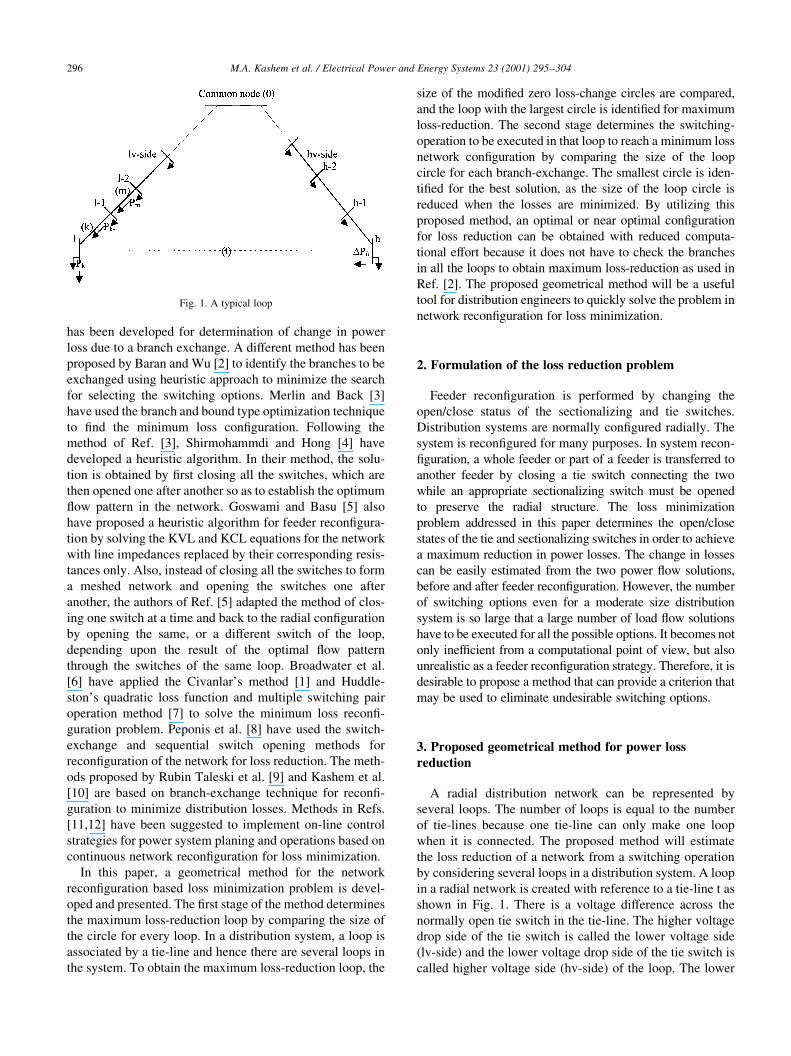
It was mentioned that the individual branch power ¯ow

(Pm, Qm) in the loop are represented as several points in the

P±Q plane. The zero-loss change loop circle is redrawn

separately in Fig. 3 to show that if losses are reduced,

then the radius of the circle is reduced and if losses are

increased, the radius is increased. It can be visualized that

losses are reduced for those points which are inside the zero-

loss change loop circle. S (Pm, Qm) is such a point inside the

circle and C (P0, Q0) is the center of the circle. Therefore, in

the periphery of the circle, loss-reduction DLPtm � 0; inside

the circle, DLPtm . 0 and outside the circle, DLPtm , 0:

The above technique is applied to ®nd the branch asso-

ciated with sectionalizing switch to be exchanged with tie-

line at which the sizes of the circles drawn for every possible

switching operation are compared. The smallest circle is

considered the best for maximum loss-reduction and is

chosen to minimize losses by exchanging the corresponding

branch with the tie-line.

3.1. Determination of the maximum loss reduction loop

Network recon®guration for optimal or near optimal

con®guration can be achieved by performing the switching

operations on the feeders. These switching-operations are

determined by implementing a minimal tree-search of possi-

ble con®gurations. The feasible solution among all possible

trees involves a selection which maximizes the loss-reduc-

tion without violating the constraints such as voltage, capa-

city of lines/and transformers and reliability constraints. The

basic idea of the proposed search scheme is ®rst to identify

the maximum loss-reduction loop in the network and then a

switching-option is determined for the loop that gives a

maximum loss reduction.

Eq. (2) can be rearranged as

DLPtm � �A2 1 B2�=C 2 C{�Pm 2 A=C�2 1 �Qm 2 B=C�2}

�7�From Eq. (7), it is evident that the change in loss, DLPtm will

be maximum when Pm � A=C and Qm � B=C: Therefore,

the maximum value of DLPtm in a loop is

DLPtm loop � �A2 1 B2�=C �8�Rearranging Eq. (3), we get the modi®ed zero-loss

change circle as

P 0m 2A���Cp

� �2

1 Q 0m 2B���Cp

� �2

� A2 1 B2���Cp �9�

where P 0m ����Cp

Pm and Q 0m ����Cp

Qm:

The radius of the above circle is ��A2 1 B2=C��1=2; which

is the square root of DLPtm loop value in Eq. (8). The modi®ed

zero-loss change loop circles can be drawn using Eq. (9) for

M.A. Kashem et al. / Electrical Power and Energy Systems 23 (2001) 295±304298

Fig. 2. Zero loss change circles as a function of power transfer

Fig. 3. Zero loss-change loop circle

all the loops in the system and the largest circle will give the

maximum loss reduction loop among all the circles drawn

for all the loops in the network.

The drawback of Eq. (8) is that the value of the DLPtm loop

is always a positive constant for a particular loop as it is

independent of Pm and Qm. However, loss-reduction

depends on the value of DLPtm, i.e. if it is positive, losses

are reduced and if it is negative, losses are increased [2].

Whether the loss is reduced or increased cannot be shown by

Eq. (8) because it is always positive. Therefore, to ensure

that the largest circle gives the maximum loss reduction, the

nominal branch is considered. The nominal branch is the

®rst adjacent branch to the tie branch on the lv-side of

the loop and the nominal loss is the loss which occurs by

exchanging the open branch with the nominal branch. If the

nominal loss is negative, then there is no branch in the loop

that can be a candidate for branch exchange [2]. If the

nominal loss is positive, it means that loss reduction can

be achieved and the branch in the loop for branch exchange

is determined.

Eq. (7) can be rewritten for nominal branch exchange as

DLPtk � �A2 1 B2�=C 2 C{�Pk 2 A=C�2 1 �Qk 2 B=C�2}

�10�where, Pk and Qk are the power ¯ows in the nominal branch k.

Using Eq. (10) the nominal loop circle can be drawn for

nominal branch exchange and compared with the zero loss

change circle drawn by using Eq. (3) in the respective loop.

If the nominal loop circle is reduced in size, then the

nominal loss is positive and the branch exchange in the

loop gives the maximum loss-reduction. Otherwise

the next largest circle is considered and checked as above.

3.2. Determination of switching-option for loss reduction

Network recon®guration is implemented by closing a

single tie switch and opening a single sectionalizing switch

to conserve the radial structure of the feeders. A switching-

option is carried out between a tie and a sectionalizing

switch. Multiple switching-options are possible for optimal

or near optimal con®guration where several tie and sectio-

nalizing switches are simultaneously closed and/or opened

by the successive application of the proposed scheme. The

best switching-option to be implemented is chosen in each

successive operation that minimizes losses the most, with-

out any constraint violation.

Civanlar and Grainger [1] have established a rule for the

switching exchange of switches by considering the lv and

hv-side of the loop. In Ref. [1], loss reduction is achieved

when loads are transferred from the lv-side of a loop to the

hv-side of that loop. It was noted that each line contains a

sectionalizing switch to be operated for network recon®-

guration. Therefore, switching-option can also be referred

to as branch-exchange, as an open branch (tie-line) is

exchanged with a closed branch by a switching operation.

In this paper also, branches of lv-side of a loop are consid-

ered for branch exchange and the most suitable switching-

exchange is found by the proposed method as described

below.

After determining the loop that would give the maximum

loss-reduction by the procedure described in the previous

section, a branch-exchange is identi®ed in that loop. The

sizes of various circles are compared which are obtained

by using Eq. (2) for all the branches in the lv-side of the

loop. The size of the circle depends on the value of the

DLPtm. It gets reduced as the DLPtm value is positive and

increased if DLPtm is negative. When DLPtm is positive

maximum for a branch-exchange, then the corresponding

circle will be the smallest one. Therefore, the smallest circle

will give the best solution and the corresponding branch-

exchange will give the maximum loss-reduction. A search

for the selection of the best branch-exchange is made by

determining and comparing the radii of the loop circles

(Eq. (2)) starting from the nominal branch k and moving

backward in the lv-side of the selected loop until the radius

of the circle is found minimum with all constraints satis®ed.

In this way, the proposed method determines the appropriate

switching-option that minimizes the losses.

4. Solution technique

The procedure to determine the loop, which gives the

maximum loss reduction, is summarized below:

(i) Run the load ¯ow program to obtain the estimates of

the power ¯ows in the branches.

(ii) Determine the radii of the modi®ed zero-loss change

circles for all the loops in the system (Eq. (9)) and

compare. Select the largest circle and the corresponding

loop.

(iii) Check the nominal branch-exchange in the selected

loop whether it contributes positive loss-reduction or not.

This is done by comparing the radius of the nominal loop

circle (Eq. (10)) with the radius of zero-loss change circle

(Eq. (3)). If nominal loop circle is reduced in size, then go

to step (v). Otherwise select the next largest circle and

repeat step (iii).

(iv) If all the nominal loop circles are increased in size

compared to their respective zero-loss change circles,

then stop.

(v) Identify the loop of the corresponding circle and

declare it as the maximum loss-reduction loop. Having

found the loop which would give the maximum loss

reduction, the next step is to determine the branch to be

exchanged.

(vi) Start from the nominal branch of the selected loop in

step (v) and search the branches backward on the lower

voltage-side of the loop until the radius of the loop circle

(Eq. (2)) is found to be minimum. Identify the corre-

sponding branch-exchange.

(vii) Check the selected branch-exchange for constraints

M.A. Kashem et al. / Electrical Power and Energy Systems 23 (2001) 295±304 299

violation. If all the constraints are satis®ed, go to step

(viii); otherwise discard the selected branch-exchange

and continue the search forward and backward (one by

one), until the constraints are satis®ed and the radius is

found to be minimum.

(viii) Declare the selected branch-exchange for maximum

loss reduction.

(ix) Repeat steps (i) to (viii) using the selected branch-

exchange.

5. Test results and discussion

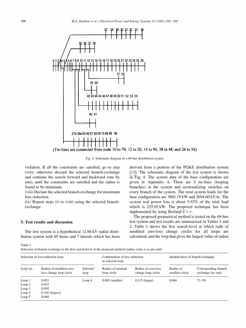
The test system is a hypothetical 12.66 kV radial distri-

bution system with 69 buses and 7 laterals which has been

derived from a portion of the PG&E distribution system

[13]. The schematic diagram of the test system is shown

in Fig. 4. The system data of the base con®guration are

given in Appendix A. There are 5 tie-lines (looping

branches) in the system and sectionalizing switches on

every branch of the system. The total system loads for the

base con®guration are 3802.19 kW and 2694.60 kVAr. The

system real power loss is about 5.92% of the total load

which is 225.05 kW. The proposed technique has been

implemented by using Borland C11.

The proposed geometrical method is tested on the 69-bus

test system and test results are summarized in Tables 1 and

2. Table 1 shows the ®rst search-level at which radii of

modi®ed zero-loss change circles for all loops are

calculated, and the loop that gives the largest value of radius

M.A. Kashem et al. / Electrical Power and Energy Systems 23 (2001) 295±304300

Fig. 4. Schematic diagram of a 69-bus distribution system

Table 1

Selection of branch-exchange in the ®rst search-level of the proposed method (radius value is in per unit)

Selection of loss-reduction loop Con®rmation of loss reduction

in selected loop

Identi®cation of branch-exchange

Loop no. Radius of modi®ed zero-

loss change loop circle

Selected

loop

Radius of nominal

loop circle

Radius of zero-loss

change loop circle

Radius of

smallest circle

Corresponding branch-

exchange (in±out)

Loop 1 0.051 Loop 4 0.005 (smaller) 0.115 (larger) 0.004 73±59

Loop 2 0.015

Loop 3 0.050

Loop 4 0.105 (largest)

Loop 5 0.040

is selected. In the next step, a comparison is made between

the nominal loop circle and the zero-loss change loop circle

to make sure that the selected loop gives loss reduction. The

nominal circle has to be smaller to achieve loss reduction in

the system. Finally, the branch-exchange in that loop is

selected by determining and comparing the radii of the

loop circles starting from the nominal branch and searching

the branches backward in the lv-side of the selected loop

until the smallest circle is found which gives the maximum

loss-reduction. As shown in Table 1, the ®rst iteration of the

proposed method has found loop 4 as the maximum loss-

reduction loop, and the branch exchange 73±59 to be

performed in that loop to achieve maximum loss reduction.

The above procedure is continued until all the loops have

the nominal circles larger compared to their respective zero-

loss change circles.

Table 2 shows the summary of the selection of branch-

exchanges in all the search-levels of the proposed method.

The optimal network con®guration for loss reduction is

achieved after ®ve search-levels of the proposed method,

in which, at each search level (or iteration) a load ¯ow

solution is obtained, the maximum loss-reduction loop is

selected and a branch-exchange is determined. In the ®fth

search-level, all the nominal circles become larger in size

compared to their respective zero-loss change circles and

are shown in Table 2.

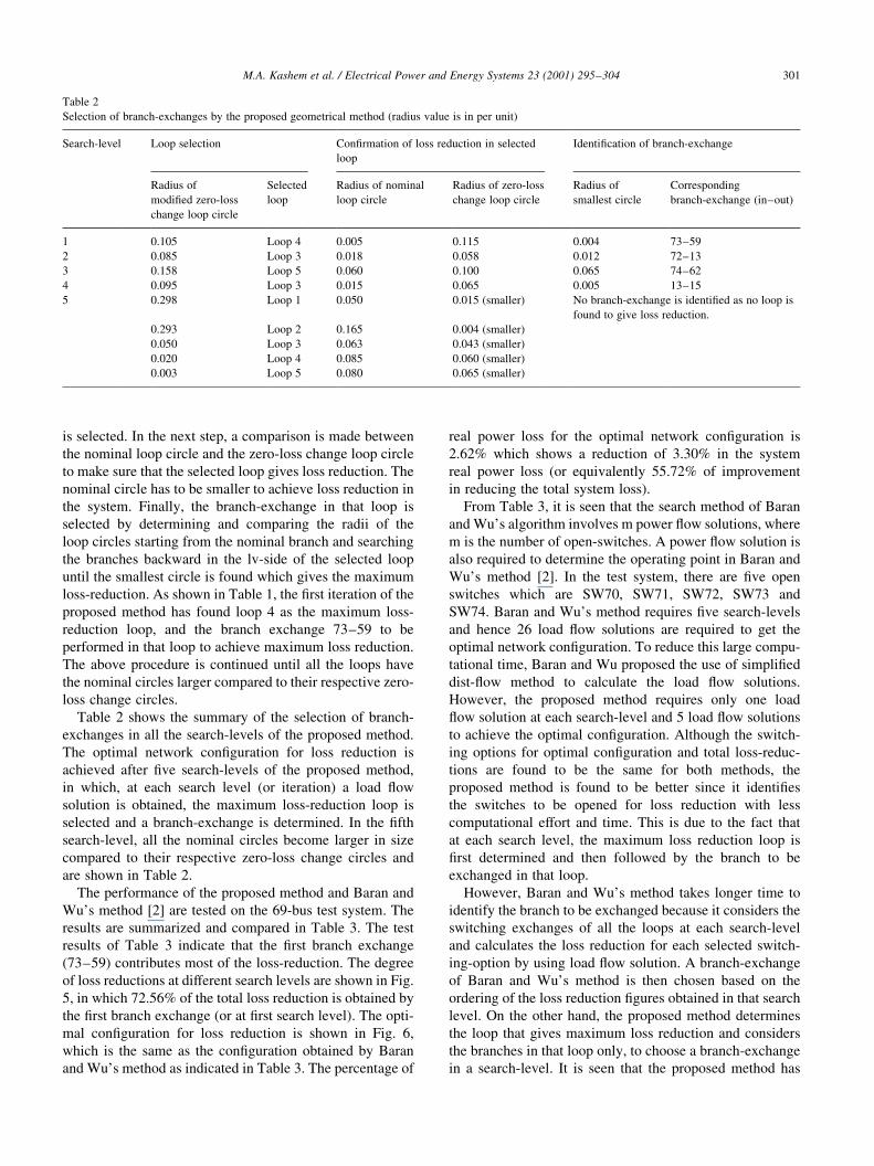
The performance of the proposed method and Baran and

Wu's method [2] are tested on the 69-bus test system. The

results are summarized and compared in Table 3. The test

results of Table 3 indicate that the ®rst branch exchange

(73±59) contributes most of the loss-reduction. The degree

of loss reductions at different search levels are shown in Fig.

5, in which 72.56% of the total loss reduction is obtained by

the ®rst branch exchange (or at ®rst search level). The opti-

mal con®guration for loss reduction is shown in Fig. 6,

which is the same as the con®guration obtained by Baran

and Wu's method as indicated in Table 3. The percentage of

real power loss for the optimal network con®guration is

2.62% which shows a reduction of 3.30% in the system

real power loss (or equivalently 55.72% of improvement

in reducing the total system loss).

From Table 3, it is seen that the search method of Baran

and Wu's algorithm involves m power ¯ow solutions, where

m is the number of open-switches. A power ¯ow solution is

also required to determine the operating point in Baran and

Wu's method [2]. In the test system, there are ®ve open

switches which are SW70, SW71, SW72, SW73 and

SW74. Baran and Wu's method requires ®ve search-levels

and hence 26 load ¯ow solutions are required to get the

optimal network con®guration. To reduce this large compu-

tational time, Baran and Wu proposed the use of simpli®ed

dist-¯ow method to calculate the load ¯ow solutions.

However, the proposed method requires only one load

¯ow solution at each search-level and 5 load ¯ow solutions

to achieve the optimal con®guration. Although the switch-

ing options for optimal con®guration and total loss-reduc-

tions are found to be the same for both methods, the

proposed method is found to be better since it identi®es

the switches to be opened for loss reduction with less

computational effort and time. This is due to the fact that

at each search level, the maximum loss reduction loop is

®rst determined and then followed by the branch to be

exchanged in that loop.

However, Baran and Wu's method takes longer time to

identify the branch to be exchanged because it considers the

switching exchanges of all the loops at each search-level

and calculates the loss reduction for each selected switch-

ing-option by using load ¯ow solution. A branch-exchange

of Baran and Wu's method is then chosen based on the

ordering of the loss reduction ®gures obtained in that search

level. On the other hand, the proposed method determines

the loop that gives maximum loss reduction and considers

the branches in that loop only, to choose a branch-exchange

in a search-level. It is seen that the proposed method has

M.A. Kashem et al. / Electrical Power and Energy Systems 23 (2001) 295±304 301

Table 2

Selection of branch-exchanges by the proposed geometrical method (radius value is in per unit)

Search-level Loop selection Con®rmation of loss reduction in selected

loop

Identi®cation of branch-exchange

Radius of

modi®ed zero-loss

change loop circle

Selected

loop

Radius of nominal

loop circle

Radius of zero-loss

change loop circle

Radius of

smallest circle

Corresponding

branch-exchange (in±out)

1 0.105 Loop 4 0.005 0.115 0.004 73±59

2 0.085 Loop 3 0.018 0.058 0.012 72±13

3 0.158 Loop 5 0.060 0.100 0.065 74±62

4 0.095 Loop 3 0.015 0.065 0.005 13±15

5 0.298 Loop 1 0.050 0.015 (smaller) No branch-exchange is identi®ed as no loop is

found to give loss reduction.

0.293 Loop 2 0.165 0.004 (smaller)

0.050 Loop 3 0.063 0.043 (smaller)

0.020 Loop 4 0.085 0.060 (smaller)

0.003 Loop 5 0.080 0.065 (smaller)

greatly reduced the computational time compared to Baran

and Wu's method due to the less number of load ¯ow execu-

tions. It is experimentally proven that the methods involved

with a large number of load ¯ow solutions, some times,

seem exhaustive and unrealistic especially for larger

systems, due to excessive computational time.

6. Conclusion

A geometrical method for loss-reduction has been

presented in this paper. In the ®rst stage of the proposed

method, the sizes of the modi®ed zero-loss change circles

are compared, and the largest one is selected as the maxi-

mum loss-reduction loop. To ensure the loss-reduction for a

branch-exchange in the selected loop, the size of nominal

loop circle is compared with that of the zero-loss change

circle. If the nominal loop circle-size is reduced, then the

corresponding loop gives the maximum loss reduction.

Otherwise, the next largest circle is considered. In the

next stage, the sizes of the loop circles for various branch-

exchanges in the selected loop are compared to identify the

smallest one for the best solution. The corresponding

branch-exchange of the smallest circle gives the maximum

loss-reduction in the system. To show the ef®ciency and

performance of the proposed method for the solution of

computationally complex and large dimensionality

problems, a system with 69-bus and seven laterals has

been considered. Test results indicate that the proposed

method can identify the most effective branch-exchange

operations for loss-reduction with less computational effort

and time. A new approach for network recon®guration

based loss reduction is presented in this paper by

introducing a geometrical technique. The method can be

M.A. Kashem et al. / Electrical Power and Energy Systems 23 (2001) 295±304302

Table 3

Results obtained by the proposed geometrical method and Baran and Wu's Method [2] (`(in±out)' indicates branch into the system and branch out from the

system, respectively)

Search level Proposed geometrical method Baran and Wu's branch±exchange method

Maximum loss

reduction loopa

Branch exchange

(in±out)

Loss reduction

(kW)

Branch exchange

(in±out)

Loss reduction

(kW)

Chosen

branch-exchange

1 Loop 4 73±59 90.98 70±10 29.94 73±59

71±18 2.96

72±12 28.84

73±59 90.98

74±62 24.21

2 Loop 3 72±13 11.08 70±11 2.70 72±13

71±18 2.76

72±13 11.08

59±73 290.98

74±62 4.32

3 Loop 5 74±62 23.13 70±11 22.19 74±62

71±21 20.18

13±15 20.07

59±73 277.70

74±62 23.13

4 Loop 3 13±15 0.20 70±43 221.93 13±15

71±21 22.31

13±15 0.20

59±73 249.89

62±61 2224.33

5 No loop is selected

for loss reductionb

± ± 70±43 221.79 No branch-

exchange

is selectedc

71±21 26.68

15±72 230.09

59±73 250.34

62±61 2222.73

Selection of ®nal

branch-exchange

Selection of ®nal branch-exchange

73±59, 72±15, 74±62 73±59, 72±15, 74±62

a Loop1 is associated with tie-line 70, loop2 with tie-line 71, loop3 with tie-line 72, loop4 with tie-line 73 and loop5 with tie-line 74.b No loop is selected in the search for loss reduction due to all nominal circles becoming bigger in size compared to their respective zero-loss change circles.c No branch exchange is selected because of negative loss reduction for all branch-exchanges.

implemented in two distinct ways: one is by measuring and

comparing the radii of the circles as presented in this paper,

and the other is by drawing, superimposing and comparing

the circles graphically. The proposed method can be used as

an ef®cient tool for network recon®guration based loss-

reduction in distribution systems.

Acknowledgements

Some of the preliminary results of this paper have been

reported in International Power Engineering Conference

(IPEC '99), Singapore, 24±26 May 1999.

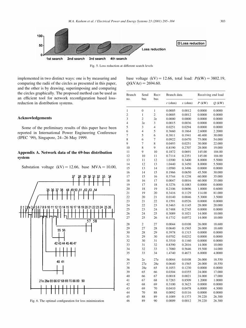
Appendix A. Network data of the 69-bus distributionsystem

Substation voltage (kV)� 12.66, base MVA� 10.00,

base voltage (kV)� 12.66, total load: P(kW)� 3802.19,

Q(kVAr)� 2694.60.

M.A. Kashem et al. / Electrical Power and Energy Systems 23 (2001) 295±304 303

Fig. 5. Loss reduction at different search levels

Fig. 6. The optimal con®guration for loss minimization

Branch

no.

Send

bus

Recv

bus

Branch data Receiving end load

r (ohm) x (ohm) P (kW) Q (kW)

1 0 1 0.0005 0.0012 0.0000 0.0000

2 1 2 0.0005 0.0012 0.0000 0.0000

3 2 2e 0.0000 0.0000 0.0000 0.0000

4 2e 3 0.0015 0.0036 0.0000 0.0000

5 3 4 0.0251 0.0294 0.0000 0.0000

6 4 5 0.3660 0.1864 2.6000 2.2000

7 5 6 0.3811 0.1941 40.400 30.000

8 6 7 0.0922 0.0470 75.000 54.000

9 7 8 0.0493 0.0251 30.000 22.000

10 8 9 0.8190 0.2707 28.000 19.000

11 9 10 0.1872 0.0691 145.00 104.00

12 10 11 0.7114 0.2351 145.00 104.00

13 11 12 1.0300 0.3400 8.0000 5.5000

14 12 13 1.0440 0.3450 8.0000 5.5000

15 13 14 1.0580 0.3496 0.0000 0.0000

16 14 15 0.1966 0.0650 45.500 30.000

17 15 16 0.3744 0.1238 60.000 35.000

18 16 17 0.0047 0.0016 60.000 35.000

19 17 18 0.3276 0.1083 0.0000 0.0000

20 18 19 0.2106 0.0696 1.0000 0.6000

21 19 20 0.3416 0.1129 114.00 81.000

22 20 21 0.0140 0.0046 5.3000 3.5000

23 21 22 0.1591 0.0526 0.0000 0.0000

24 22 23 0.3463 0.1145 28.000 20.000

25 23 24 0.7488 0.2745 0.0000 0.0000

26 24 25 0.3089 0.1021 14.000 10.000

27 25 26 0.1732 0.0572 14.000 10.000

28 2 27 0.0044 0.0108 26.000 18.600

29 27 28 0.0640 0.1565 26.000 18.600

30 28 29 0.3978 0.1315 0.0000 0.0000

31 29 30 0.0702 0.0232 0.0000 0.0000

32 30 31 0.3510 0.1160 0.0000 0.0000

33 31 32 0.8390 0.2816 14.000 10.000

34 32 33 1.7080 0.5646 19.500 14.000

35 33 34 1.4740 0.4673 6.0000 4.0000

36 2e 27e 0.0044 0.0108 26.000 18.550

37 27e 28e 0.0640 0.1565 26.000 18.550

38 28e 65 0.1053 0.1230 0.0000 0.0000

39 65 66 0.0304 0.0355 24.000 17.000

40 66 67 0.0018 0.0021 24.000 17.000

41 67 68 0.7283 0.8509 1.2000 1.0000

42 68 69 0.3100 0.3623 0.0000 0.0000

43 69 70 0.0410 0.0478 6.0000 4.3000

44 70 88 0.0092 0.0116 0.0000 0.0000

45 88 89 0.1089 0.1373 39.220 26.300

46 89 90 0.0009 0.0012 39.220 26.300

References

[1] Civanlar S, Grainger JJ, Yin H, Lee SSH. Distribution feeder recon-

®guration for loss reduction. IEEE Transactions on Power Delivery

1988;3(3):1217±23.

[2] Baran ME, Wu FF. Network recon®guration in distribution systems

for loss reduction and load balancing. IEEE Transactions on Power

Delivery 1989;4(2):1401±7.

[3] Merlin A, Back H. Search for a minimal-loss operating spanning tree

con®guration for an urban power distribution system. Proceedings of

the Fifth Power System Conference (PSCC). Cambridge, 1975. p. 1±

18.

[4] Shirmohammadi D, Hong HW. Recon®guration of electric distribu-

tion networks for resistive line losses reduction. IEEE Transactions on

Power Delivery 1989;4(2):1492±8.

[5] Goswami SK, Basu SK. A new algorithm for the recon®guration of

distribution feeders for loss minimization. IEEE Transactions on

Power Delivery 1992;7(3):1484±91.

[6] Broadwater RP, Khan AH, Shaalan HE, Lee RE. Time varying load

analysis to reduce distribution losses through recon®guration. IEEE

Transactions on Power Delivery 1993;8(1):294±300.

[7] Huddleston CT, Broadwater RP, Chandrasekaran A. Recon®guration

algorithm for minimizing losses in radial electric distribution systems.

Electric Power System Research 1990;18(1):57±67.

[8] Peponis GP, Papadopoulos MP, Hatziargyriou ND. Distribution

network recon®guration to minimize resistive line losses. IEEE

Transactions on Power Delivery 1995;10(3):1338±42.

[9] Taleski R, Rajicic D. Distribution network recon®guration for energy

loss reduction. IEEE Transactions on Power Systems 1997;12(1):

398±406.

[10] Kashem MA, Moghavvemi M, Mohamed A, Jasmon GB. Loss reduc-

tion in distribution networks using new network recon®guration algo-

rithm. Electric Machines and Power Systems 1998;26(8):815±29.

[11] Shin BCG. Development of the loss minimization function for real

time power system operations: a new tool. IEEE Transactions on

Power Systems 1994;9(4):2028±34.

[12] Borozan V, Rajakovic N. Minimum loss distribution network con®g-

uration: analyses and management. Proceedings of IEE Conference,

2±5 June 1997. p. 6.18.1±6.18.5.

[13] Baran ME, Wu FF. Optimal capacitor placement on radial distribution

systems. IEEE Transactions on Power Delivery 1989;4(1):725±34.

M.A. Kashem et al. / Electrical Power and Energy Systems 23 (2001) 295±304304

(continued)

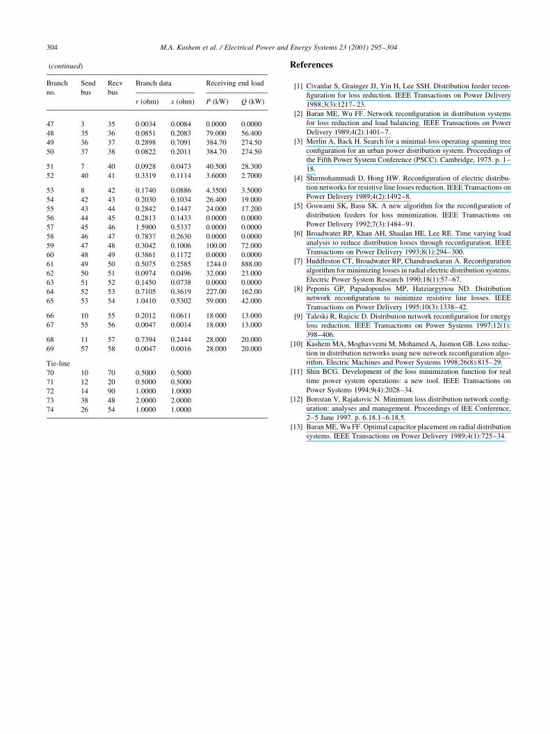
Branch

no.

Send

bus

Recv

bus

Branch data Receiving end load

r (ohm) x (ohm) P (kW) Q (kW)

47 3 35 0.0034 0.0084 0.0000 0.0000

48 35 36 0.0851 0.2083 79.000 56.400

49 36 37 0.2898 0.7091 384.70 274.50

50 37 38 0.0822 0.2011 384.70 274.50

51 7 40 0.0928 0.0473 40.500 28.300

52 40 41 0.3319 0.1114 3.6000 2.7000

53 8 42 0.1740 0.0886 4.3500 3.5000

54 42 43 0.2030 0.1034 26.400 19.000

55 43 44 0.2842 0.1447 24.000 17.200

56 44 45 0.2813 0.1433 0.0000 0.0000

57 45 46 1.5900 0.5337 0.0000 0.0000

58 46 47 0.7837 0.2630 0.0000 0.0000

59 47 48 0.3042 0.1006 100.00 72.000

60 48 49 0.3861 0.1172 0.0000 0.0000

61 49 50 0.5075 0.2585 1244.0 888.00

62 50 51 0.0974 0.0496 32.000 23.000

63 51 52 0.1450 0.0738 0.0000 0.0000

64 52 53 0.7105 0.3619 227.00 162.00

65 53 54 1.0410 0.5302 59.000 42.000

66 10 55 0.2012 0.0611 18.000 13.000

67 55 56 0.0047 0.0014 18.000 13.000

68 11 57 0.7394 0.2444 28.000 20.000

69 57 58 0.0047 0.0016 28.000 20.000

Tie-line

70 10 70 0.5000 0.5000

71 12 20 0.5000 0.5000

72 14 90 1.0000 1.0000

73 38 48 2.0000 2.0000

74 26 54 1.0000 1.0000