Characteristics of the turbulent/nonturbulent interface in boundary layers, jets and shear-free...

This content has been downloaded from IOPscience. Please scroll down to see the full text.

Download details:

IP Address: 135.84.214.170

This content was downloaded on 31/01/2016 at 11:13

Please note that terms and conditions apply.

Characteristics of the turbulent/nonturbulent interface in boundary layers, jets and shear-free

turbulence

View the table of contents for this issue, or go to the journal homepage for more

2014 J. Phys.: Conf. Ser. 506 012015

(http://iopscience.iop.org/1742-6596/506/1/012015)

Home Search Collections Journals About Contact us My IOPscience

iopscience.iop.org/page/terms

http://iopscience.iop.org/1742-6596/506/1

http://iopscience.iop.org/1742-6596

http://iopscience.iop.org/

http://iopscience.iop.org/search

http://iopscience.iop.org/collections

http://iopscience.iop.org/journals

http://iopscience.iop.org/page/aboutioppublishing

http://iopscience.iop.org/contact

http://iopscience.iop.org/myiopscience

Characteristics of the turbulent/nonturbulent

interface in boundary layers, jets and shear-free

turbulence

Carlos B. da Silva1, Rodrigo R. Taveira1, Guillem Borrell2

1Department of Mechanical Engineering. Instituto Superior Tecnico. Lisboa. Portugal2ETSI Aeronauticos. Universidad Politecnica de Madrid. Madrid. Spain

E-mail: [email protected]

Abstract. The characteristics of turbulent/nonturbulent interfaces (TNTI) from boundarylayers, jets and shear-free turbulence are compared using direct numerical simulations. TheTNTI location is detected by assessing the volume of turbulent flow as function of the vorticitymagnitude and is shown to be equivalent to other procedures using a scalar field. Vorticitymaps show that the boundary layer contains a larger range of scales at the interface than injets and shear-free turbulence where the change in vorticity characteristics across the TNTI ismuch more dramatic. The intermittency parameter shows that the extent of the intermittencyregion for jets and boundary layers is similar and is much bigger than in shear-free turbulence,and can be used to compute the vorticity threshold defining the TNTI location. The statisticsof the vorticity jump across the TNTI exhibit the imprint of a large range of scales, from theKolmogorov micro-scale to scales much bigger than the Taylor scale. Finally, it is shown thatcontrary to the classical view, the low-vorticity spots inside the jet are statistically similar toisotropic turbulence, suggesting that engulfing pockets simply do not exist in jets.

1. IntroductionIn many turbulent shear flows such as boundary layers, jets, mixing layers and wakes there isa sharp interface that divides the flow field into two distinct regions. In one region the flow isturbulent while in the other, the flow is largely irrotational (Corrsin and Kistler [1]). This sharpinterface - the turbulent/nonturbulent interface (TNTI) – is continually deformed over a widerange of scales and the flow dynamics in its vicinity determines many of the most importantflow features: the growth and spreading rate of wakes, the exchanges of mass across mixinglayers, and the mixing and reaction rates in jets are some of the flow features that are largelydetermined by the characteristics of the TNTI and the flow dynamics in its vicinity.

The key event that occurs at a TNTI is the ‘communication’ of vorticity from the core of theturbulent region into the irrotational zone. Turbulent entrainment can be seen as the mechanismby which fluid elements from the irrotational flow region acquire vorticity and become part ofthe turbulent region. Past studies described the entrainment as being caused by large-scale eddymotions (engulfment) occurring from time to time at particular locations along the TNTI [2], butrecent works suggest instead that the entrainment results from small scale motions (nibbling)acting along the entire TNTI (Mathew and Basu [3], Hunt et al.[4]), as originally described byCorrsin and Kistler [1].

1st Multiflow Summer Workshop IOP PublishingJournal of Physics: Conference Series 506 (2014) 012015 doi:10.1088/1742-6596/506/1/012015

Content from this work may be used under the terms of the Creative Commons Attribution 3.0 licence. Any further distributionof this work must maintain attribution to the author(s) and the title of the work, journal citation and DOI.

Published under licence by IOP Publishing Ltd 1

The flow dynamics near the TNTI has been assessed in several recent works and it has beenobserved that many flow variables, e.g., velocity and vorticity display characteristic (sharp)jumps at the TNTI (Westwerweel et al. [5], Holzner et al. [6], da Silva and Pereira [7]), and thedynamics of the vorticity and kinetic energy have been analysed near the TNTI to understandthese jumps (e.g. Holzner et al. [6], Taveira and da Silva [8], Taveira et al. [9]).

Links between geometry and dynamics are often not straightforward, but several studieshave addressed the geometrical characteristics of TNTIs from different flows. It is know fromnumerous experimental observations that the TNTI is sharp and is continually distorted at alarge range of scales by the turbulent structures in its vicinity (Corrsin and Kistler [1], Townsend[2]). The largest convolutions observed at the TNTI are the imprint of the largest-scale eddiesfrom the turbulent region, which move at a speed imposed by their characteristic velocity andthe integral scale L11 from the turbulent region (Townsend [10]). Statistics of the TNTI positionyi were assessed in numerous works starting with Corrsin and Kistler [1]. They concluded thatyi is approximately Gaussian, a result that has been remarked in numerous works since thene.g. Gampert et al. [11]. However, La Rue and Libby have measured the forward and backwardslopes of the TNTI using experimental data in the wake of a heated cylinder, and observed thatthese slopes are different, which is inconsistent with Gaussian distribution of yi. The convex andconcave regions of the TNTI were assessed recently in experimental turbulent jets by Wolf et al.[12] and it was realised that depending on the surface shape, different small-scale mechanismsare dominant for the local entrainment process.

The geometry of the TNTI has also been linked to the flow structures underneath e.g. daSilva and Reis [13] analysed the coherent vortices near the TNTI and observed that large vorticalstructures are responsible for the existence of positive enstrophy diffusion along the interfacelayer, linking the results of Holzner et al. [6] to the large-scale vorticity structures. Moreover,the characteristic vorticity jump observed in different flows has been linked to the eddy structurenear the TNTI (da Silva and Taveira [14]), and the dynamics of the small-scale intense vorticitystructures neighbouring the TNTI suggests that the nibbling eddy motions are linked to thediffusion of vorticity from these small scale vortices near the TNTI (da Silva et al. [15]).

Another geometrical feature of the TNTI is its fractal character. Indeed, the appealing ideathat turbulence exhibits a scale-invariant (or fractal) character has lead to much research firedby the new ideas beautifully presented by Mandelbrot [16]. Numerous past experimental andsome numerical works have searched for the (self-similar) fractal features of lines and surfaceswithin turbulent flows. The TNTI defined using the vorticity or a passive scalar supported theexistence of a range of scales exhibiting self-similar fractal dimension between D2 ≈ 2.3− 2.4 innumerous different flows (Sreenivasan [17]). However, many works have also raised doubts onthe self-similar character, suggesting instead a more complex scale-dependent fractal dimensioni.e. multifractal behaviour for some variables (Frederiksen et al. [18], Catrakis [19]), but recentwork based on experimental data from boundary layers is consistent with the TNTI being aself-similar fractal with D2 ≈ 2.3− 2.4 (de Silva et al. [20]).

Even though several geometrical aspects of TNTI have been analysed in the past, nosystematic work addressed the differences and similarities from TNTIs in different flows. Thiswork presents a first attempt at such a study. The data banks analysed here comprise directnumerical simulations (DNS) of boundary layers, planar jets and shear-free turbulence. In allthe simulations, the Reynolds number based on the Taylor micro-scale is slightly greater thanReλ ≈ 100, the main differences being the boundary and initial conditions, the existence orabsence of mean shear, or the proximity of the mean shear to the location of the TNTI.

This article is organised as follows. In section 2 we describe the DNS used in the presentwork. Section 3 analyses the detection of the TNTI based in the volume of the turbulent regionand relates this method with other procedures used in experimental works. The vorticity mapsfor the three simulations are compared. Section 4 shows visualisations of the TNTIs in boundary


2

Figure 1: Sketch of the simulation, presenting the dual configuration with an auxiliary boundary layer.

Case Nx, Ny, Nz Reθ Reλ δ99/η δ99/λ

BLaux 3585× 315× 2560 1100− 2970 − − −BL 15361× 535× 4096 2780− 6650 75− 125 2600− 4400 15− 21

Table 1: Parameters of the boundary layer simulation. Nx, Ny and Nz are the computational domainsize. The following columns correspond to the values at the beginning and at the end of the simulationdomain that is considered correct. Given that both the Kolmogorov (η) and Taylor (λ) scales changedepending on the distance to the wall, a reference height y = 0.6δ99 has been chosen.

layers and jets. Section 5 compares the intermittency characteristics and associated length scalesin the three flows analysed here, while section 6 discusses the thickness of the local vorticityjump in jets. Finally, in section 7 the geometry of the irrotational bubbles that are found inside ajet is investigated. The work ends with an overview of the main results and conclusions (section8).

2. Description of the data setsAll the data used in this study have been obtained from Direct Numerical Simulation (DNS).Thanks to recent advances in particle image velocimetry [21] (PIV), and particle trackingvelocimetry [6] (PTV), experimental techniques are able to capture the interface with accuracy,and to obtain the properties of the flow at the same time, but one important advantage of DNSover experimental techniques is its dynamic range, and in consequence, the ability to capture allthe relevant scales in each case. Given that the goal of this study is to compare the geometricalproperties of the interface detection in different flows, DNS data are a more reasonable choice.

Capturing all the information contained in the field comes with a cost. The separationbetween the smallest scales, given by viscosity, and the largest ones, given by the geometry ofthe problem, is proportional to the computational cost. Knowing that scale separation is crucialin the analysis of turbulent flows, this study uses some of the largest simulations available today.

2.1. Boundary layerBoundary layer data are obtained from DNS of a zero-pressure-gradient turbulent boundarylayer over a flat plate. The goal of this simulation is to obtain a range of Reynolds numberswhere all the scales have reach their equilibrium, and are free of the influence of the boundaryconditions. This goal is achieved by running two boundary layers at the same time. An auxiliarysimulation solves the flow at a lower Reynolds number, and low resolution, but with the sametime step as the primary simulation. The purpose of this auxiliary simulation is to providecorrect inflow to the second one, that can be considered correct in all its extent. A scheme ofthe dual configuration is shown in figure 1. The details of the algorithms and the methodologyare explained with detail in Simens et al. [22], and Borrell et al. [23].


3

In the boundary layer, the streamwise, wall-normal, and spanwise directions are called x, y,and z respectively. Only the principal simulation BL is used. A list of the important parametersof the dataset is presented in table 1. Detailed statistics, that agree perfectly with the previousexperiments and simulations, can be found in Sillero and Jimenez [24], where a detailed analysisof the convergence of the large scales can be found.

It is important to note that in boundary layers, some quantities that are used as a unit, likethe Kolmogorov microscale η = (ν3/ε)1/4, where ε is the energy dissipation rate, or the rootmean square of vorticity magnitude ωrms, depend on the distance to the wall. In this case, areference value at y/δ99 = 0.6 is used without taking into consideration any flow anisotropy, andthis value will be used regardless of the dependence with respect to y, to simplify the notation.When a channel at a similar Reynolds number is used for comparison, the reference value istaken at y/h = 0.6, where h is the half-height of the channel.

2.2. Planar jetA DNS of a temporally developing turbulent plane jet was used. This simulation is described indetail in Taveira and da Silva [8] (labeled as PJETchan.) and therefore only a short descriptionwill be given here. The simulation was carried out with a Navier–Stokes solver that employspseudo-spectral methods for spatial discretization and a three-step Runge–Kutta scheme fortemporal advancement. The simulation was fully dealiased using the 2/3 rule. The initialcondition consists of interpolated velocity fields from a DNS of a turbulent channel flow andthe computational domain extends to (Lx, Ly, Lz) = (6.3H, 8H, 4.2H), along the streamwise(x), normal (y), and spanwise (z) jet directions, respectively, where H is the inlet slot-widthof the jet. The simulation uses (Nx ×Ny ×Nz) = (1152 × 1536 × 768) grid points. At the farfield self-similar region (where the subsequent analysis was carried out) the Reynolds numberbased on the Taylor micro-scale λ, and on the root-mean-square of the streamwise velocity u′ isReλ = u′λ/ν ≈ 140 across the jet shear layer, and the resolution is ∆x/η ≈ 1.1.

Jets are inhomogeneous in the direction along the y coordinate. Like in the case of theboundary layer, a reference value is used for η and ωrms, taken at the centre of the jet. In thecase of a jet this is justified by the fact that the mean dissipation rate (like in the shear-freecase) is roughly constant inside the turbulent region.

2.3. Shear-free turbulenceA DNS of shear-free turbulence was carried out in a periodic box with sizes 2π and using(Nx ×Ny ×Nz) = (512× 512× 512) collocation points. The Navier–Stokes solver is essentiallythe same used in the plane jet DNS. The simulation starts by instantaneously inserting a velocityfield from a previously run DNS of forced isotropic turbulence into the middle of a field of zeroinitial velocity. As time progresses, the initial isotropic turbulence region spreads into theirrotational region in the absence of mean shear. The imposition of these initial boundaryconditions can be accomplished by drastically reducing the time step in the simulations whenthe boundary condition is inserted, as described in Perot and Moin [25]. More details on thisprocedure can be found in Teixeira and da Silva [26] where a similar simulation is reported.In the present shear-free simulation the Reynolds number based on the Taylor micro-scale isReλ ≈ 115, and the resolution is ∆x/η ≈ 1.5.

3. Detection of the turbulent/nonturbulent interfaceThe TNTI separates the turbulent from the irrotational flow regions and several methods existto detect its location e.g. Bisset et al. [27], Westerweel et al. [5]. Since by definition theirrotational region has no vorticity it is natural to define the TNTI in terms of the vorticity/no-vorticity content of the flow. In practice one looks for a low vorticity-magnitude threshold ω0,below which the flow region can be considered to be (approximately) irrotational. In several


4

0 2 4 6 8 10ω/ωrms

0.0

0.2

0.4

0.6

0.8

1.0

V(ω

0)/Vt

(a)

ω/ωrms

V(ω

0)/

Vt

0 2 4 6 8 100

0.2

0.4

0.6

0.8

1

(b)

ω/ωrms

V(ω

0)/

Vt

0 50 1000

0.2

0.4

0.6

0.8

1

(c)

Figure 2: Volume of the region with vorticity magnitude greater than a given threshold ω > ω0, asfunction of the vorticity magnitude threshold for the boundary layer (a), jet (b), and shear-free turbulence(c). ωrms is the reference rms vorticity used for each case, as described in section 2.

flows it has been observed that many statistics of the interface layer (e.g. conditional vorticityprofiles in relation to the distance from the TNTI, the geometric shape of the TNTI) are weaklydependent of the particular value assumed by ω0 if it separates reasonably well the regions ofturbulent and irrotational flow.

3.1. Detection of the turbulent/nonturbulent interface based on the volume of the turbulentregionIn the present case the method described in Taveira et al. [9] is used to compute ω0. Thismethod relies on the fact that the volume of the turbulent flow region, defined as the regionwhere the vorticity magnitude is greater than a given threshold, exhibits a particular shapewhich is illustrated in figures 2(a), 2(b) and 2(c). The figures show the volume V of theturbulent region for the boundary layer, jet and shear-free turbulence cases, respectively, asfunction of the vorticity magnitude (threshold) used to detect it: V (ωI) i.e. we designate by ωIthe particular value of ω0 obtained using the volume method. As expected the turbulent volumeis a monotonically decreasing function of the vorticity threshold, but in all three cases the rateof decrease changes with the vorticity magnitude ω. The turbulent volume falls sharply with theincrease of ω until, for a given ω, the decrease rate slows down. For the jet case this happens ataround ω/ωrms ≈ 0.3. It was observed that in practice any value of ω near this changing regioncan be used to define the location of the TNTI. The particular value of the vorticity magnitudethreshold used here ωI is defined as the inflection point of the turbulent volume

∂2V (ω > ω0)

∂ω20

∣∣∣∣∣ω0=ωI

= 0. (1)

3.2. Relation to other criteria for turbulent/non-turbulent interface detectionInterestingly the method described above is related to other methods based on the concentrationof a passive scalar field. Specifically, there is one widely used criterion to threshold scalar fieldswhere interfaces are to be found, described in [28], where it is applied to a turbulent jet. Themethod proposes to seed the turbulent side with a scalar, and assumes that the concentration ofthis scalar is an indication of how much turbulent is the fluid at each point. This hypotheticalcharacteristic of the relative concentration field φ is known not to be accurate, and depends onthe Schmidt number, but the analysis of how close this hypothesis is to reality is not a goal ofthis study.


5

10-5 10-4 10-3 10-2 10-1 100 101 1020.00

0.02

0.04

0.06

0.08

0.10

0.12

0.14

0.16

PDF

Jet

10-710-610-510-410-310-210-1 100 101 1020.00

0.05

0.10

0.15

0.20

0.25

0.30

0.35Boundary layer

10-4 10-3 10-2 10-1 100 101 102

ω/ωrms

0.00

0.01

0.02

0.03

0.04

0.05

0.06

PDF

Isotropic

10-4 10-3 10-2 10-1 100 101 102

ω/ωrms

0.00

0.05

0.10

0.15

0.20

0.25Channel

Figure 3: P.d.f. for vorticity magnitudeusing ωrms as unit. The datasetscorresponding to Channel and Isotropiccorrespond to a turbulent channel ofsize π × π/2 at Reτ = 950[29],and a box of size 5123 at Reλ =168[30] respectively. It is clear thatfully turbulent flows present only onestate, and the probability distribution ofvorticity is unimodal.

If the flow is in two different states this scalar field φ will have a bimodal probability densityfunction (p.d.f.). This means that most of the volume is either irrotational (φ ' 0) or turbulent(φ ' 1). It is reasonable to think that, if the turbulent/non-turbulent interface is a sharp front,its volume will be small. In consequence, if the interface has a characteristic value of φI , itscontribution to the p.d.f. will be small. Therefore, one can use the minimum between the twomodes of the p.d.f. as a criterion to identify the threshold. This is a method to separate the twostates of the flow on a practical way, more than a method to locate an interface. But, given thearbitrariness of the threshold definitions found in the literature, this one is particularly simpleto apply.

While this method is used frequently in experiments, where seeding is a common practice,it is very difficult to implement in simulations. However, the vorticity magnitude can beused analogously to the concentration fraction φ. In external turbulent flows, the fluid is intwo different states regarding vorticity, or in this case, vorticity magnitude. The probabilitydistribution of ω has a bimodal shape (figure 3), and a minimum that can be used as a practicalcriterion to obtain a threshold ωI .

This method is related to the volume filled by the fluid with vorticity from 0 to ωI i.e. V (ωI),that can be expressed from the p.d.f. of the vorticity magnitude, P (ω), as

V (ωI) = Vt

(1−

∫ ωI

0P (ω) dω

), (2)

where Vt is the total volume of the domain. Differentiating twice this expression gives,

∂2V (ωI)

∂ω2I

= −Vt∂P (ωI)

∂ωI(3)

which shows that the minimum of the p.d.f. corresponds to an inflection point of the functionV (ωI) (figure 4), and gives the minimum-volume threshold.

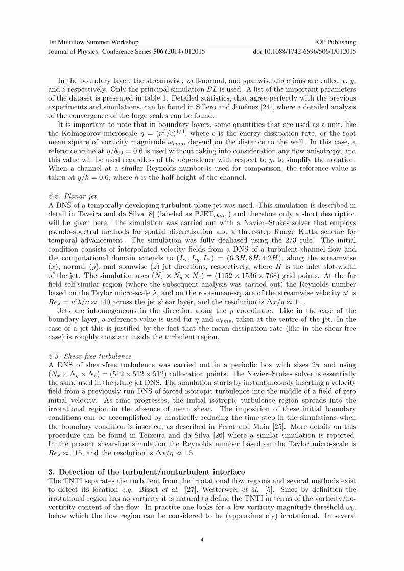
This method has several caveats. It is not clear how much the separation between the twostates of the flow is an indication to the presence of an interface, particularly because it doesnot account for the inhomogeneities of the flow. In the case of jets, strong vorticity fluctuationsexist close the turbulent/non-turbulent interface, while this is not the case in boundary layers.The centre of the jet has a region with slightly lower vorticity, with values that also contributeto the p.d.f., but no distinction is made. In the case of boundary layers, figure 3 shows that the


6

10-7 10-6 10-5 10-4 10-3 10-2 10-1 100 101 1020.00.20.40.60.81.01.21.41.61.8

PDF

Jet

Boundary Layer

10-7 10-6 10-5 10-4 10-3 10-2 10-1 100 101 102

ω/ωrms

0.0

0.2

0.4

0.6

0.8

1.0

V(ω

I)/Vt

Figure 4: P.d.f. for vorticitymagnitude (top) and volume covered bythe points where vorticity is higher thanωI (bottom) for a jet and a boundarylayer. The two curves contain the sameinformation, since they are related byequation (3). Every extrema in P (ω)corresponds to an inflection point inV (ωI)

two peaks are more separated than in the case of jets. However, it is difficult to predict theirbehaviour for higher Reynolds numbers, when vorticity has more time to decay and to adjustto the free stream.

3.3. Vorticity maps.One goal of this work is to compare the differences and similarities between the TNTIs inboundary layers, jets and shear-free turbulence. A crucial issue is to define reference locations,within the TNTI, and reference vorticity values that allow such a comparison. The difficultyarises because of the different nature of the vorticity dynamics of these flows near the TNTI,despite vorticity being a small-scale quantity that should be ‘similar’ in all flows if the Reynoldsnumber and associated separation of scales is large enough. However it is easy to understandthat the particular vorticity dynamics is quite different in the flows analysed here because thevorticity generation takes place in different regions due to different mechanism in relation tothe TNTI location. In shear-free turbulence, the vorticity is generated in the core of theturbulent region in much the same way as in isotropic turbulence, due to the interaction ofexisting fluctuating vorticity and fluctuating rate-of-strain, and is propagated without meanshear into the irrotational region across the TNTI. In the boundary layer, the wall, through theno-slip condition, provides most of the vorticity source which is then propagated away from thewall, eventually reaching the TNTI. The main source of vorticity in the boundary layer flow istherefore far from the TNTI location. Finally, in the case of the jet the situation is similar tothe shear-free turbulence case, except that the vorticity propagates into the irrotational regionacross the TNTI under the influence of mean shear. Arguably, in high-Reynolds-number jets thegeneration of a small-scale dominated quantity such as vorticity is weakly dependent on meanshear effect, but this mean shear may indirectly influence the vorticity dynamics.

An interesting way to assess the vorticity in the three flows is to represent the p.d.f. of thevorticity magnitude for every point in y (where y is a distance in the flow to be defined latter).This generates a more complicated map, that encodes more information than the intermittencyprofile, but is harder to interpret. There are two characteristic regions, one with high vorticityand another one with low vorticity, separated by almost two orders of magnitude, and connectedby the intermittent region. As will be shown below, this map allows us to give a more educatedguess about what could be a consistent value for the threshold ωI to compare the three differentflow cases.

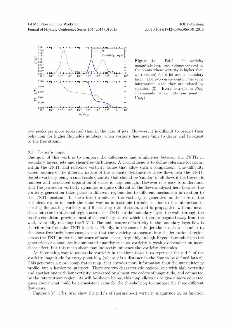
Figures 5(c), 5(b), 5(a) show the p.d.f.s of (normalised) vorticity magnitude ω∗ as function


7

of the position (y - arbitrary units) across the intermittent region. The vorticity magnitude isnormalised by ωrms in the jet and in shear-free turbulence, ω∗ = ω/ωrms, while in the boundarylayer it is normalised by a reference vorticity ωδ defined later in this section, ω∗ = ω/ωδ. Eachhorizontal line in these graphs is a p.d.f. of vorticity magnitude at a given distance e.g. fromthe wall in the case of the boundary layer (Fig. 5(a)). Starting with the shear-free turbulencecase (Fig. 5(c)) one can see that the shape of the p.d.f. clearly indicates the existence of twoflow regions. For distances smaller than y/η ≈ 102 the p.d.f. of ω∗ exhibits the same shape,with the same peak at ω∗ ≈ 1.5, while for y/η ≥ 102 the p.d.f.s are quite different, with thepeaks moving to smaller values of ω∗. The p.d.f. clearly illustrates the different behaviourof the turbulent and irrotational flow regions, with a nearly constant vorticity distribution inthe turbulent region y/η ≤ 102 and much smaller vorticity peaks in the irrotational regiony/η > 102, due to the negligible value of the vorticity magnitude there. The change observed fory/η ≈ 102 is quite dramatic in that the peak values of the p.d.f. of ω∗ are discontinuous in thedistance y, which is the consequence of a very sharp change of vorticity characteristics acrossthe intermittent region. In the jet case (Fig. 5(b)) the p.d.f.s are similar, but the ‘change incharacter’ between the turbulent and irrotational regions seems to take place across a slightlybigger distance. Finally, for the boundary layer (Fig. 5(a)) one notices that the change betweenthe turbulent and irrotational regions is less abrupt, lacking the discontinuity of the ω∗ peaks.Also, in this case, the range of values and of ω∗ seems to be larger than in the other cases andthe peaks of the p.d.f.s of ω∗ change even within the turbulent region, because of the vorticityscaling laws near the wall.

In order to compare the characteristics of TNTIs of the three flows used here we need tochoose a vorticity magnitude threshold ω0 allowing a meaningful comparison. To obtain this,figure 6(a) superimposes the above p.d.f.s in a single graph. The jet and shear-free turbulencecompare well in this figure but the boundary layer presents difficulties due to the influence ofthe wall.

The dependence with y of the r.m.s. vorticity in boundary layers can be estimated if weassume that the energy production locally balances the dissipation, and use the logarithmic-layer scaling. Expressed in wall units, ε+ ≈ ω+2 ≈ ∂yU

+ ≈ (κy+)−1, where κ is the vonKarman constant. This suggests that

Ω+(y) = (y+)−1/2 (4)

can be used as a local surrogate for ωrms in the boundary layer, to compare it with the free-shear flows. This rescaling is singular at the wall, but remains non-zero in the irrotational

region, and provides a vorticity unit at the edge of the boundary layer, ωδ = 〈ω〉wall δ−1/299 ,

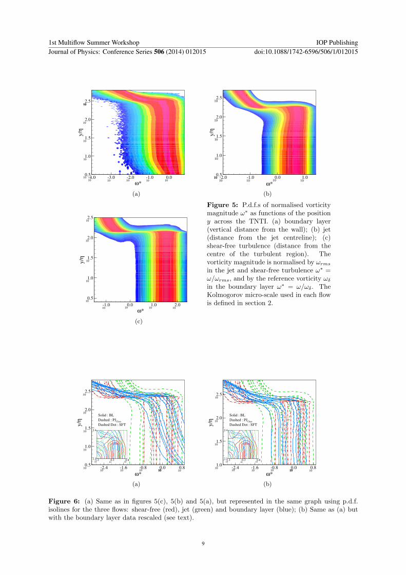
which is useful in accounting for Reynolds-number effects in studying the TNTI. Figure 6(b)shows that normalizing the vorticity fluctuations with Ω(y) rescales the turbulent part of thep.d.f.s in the intermittency maps of the three flows to similar shapes.

By comparing the p.d.f.s in figure 6(b) we see that the change in the p.d.f. characteristics inthe three flows takes place roughly at ω∗ ≈ 0.1. Therefore, in the following we will use,

ω0 = 0.1ωu (5)

as the threshold separating the turbulent from the nonturbulent regions in the three flows, whereωu stands for the unit of vorticity used in each case: ωδ in boundary layers, and ωrms in jetsand shear-free flows.

4. Visualisation of the turbulent/nonturbulent interfaceFigures 7(a) and 7(b) show iso-surfaces of vorticity magnitude corresponding to the TNTIlocation using the detection method described above. The colours indicate the local height


8

ω*

y/η

4.0 3.0 2.0 1.0 0.00.5

1.0

1.5

2.0

2.5

10

101010

10

10

1010

10 10 10 10

(a)

ω*

y/η

2.0 1.0 0.0 1.00.5

1.0

1.5

2.0

2.510

10

10

10

101010 1010 10

(b)

ω*

y/η

1.0 0.0 1.0 2.0

0.5

1.0

1.5

2.0

2.5

10

10

10

10

10

10

10 10 10

(c)

Figure 5: P.d.f.s of normalised vorticitymagnitude ω∗ as functions of the positiony across the TNTI. (a) boundary layer(vertical distance from the wall); (b) jet(distance from the jet centreline); (c)shear-free turbulence (distance from thecentre of the turbulent region). Thevorticity magnitude is normalised by ωrmsin the jet and shear-free turbulence ω∗ =ω/ωrms, and by the reference vorticity ωδin the boundary layer ω∗ = ω/ωδ. TheKolmogorov micro-scale used in each flowis defined in section 2.

ω*

y/η

2.4 1.6 0.8 0.0 0.80.5

1.0

1.5

2.0

2.5

Solid : BL

Dashed : PJChan

Dashed Dot : SFT

10

10

10

10

10

10

1010 101010

10 10

10

10

1.2 0.2 0.82.3

2.4

(a)

ω*

y/η

2.4 1.6 0.8 0.0 0.81.0

1.5

2.0

2.5

Solid : BL

Dashed : PJChan

Dashed Dot : SFT

10

10

10

10

10

10

1010 101010

10 10

10

1.2 0.2 0.82.3

2.4

(b)

Figure 6: (a) Same as in figures 5(c), 5(b) and 5(a), but represented in the same graph using p.d.f.isolines for the three flows: shear-free (red), jet (green) and boundary layer (blue); (b) Same as (a) butwith the boundary layer data rescaled (see text).


9

(a) (b)

Figure 7: Iso-surfaces of vorticity magnitude corresponding to the TNTI in the boundary layer (a) andjet (b) simulations. For the jet simulation the entire upper shear layer is displayed while only a fractionof the boundary layer is shown.

(a) (b)

Figure 8: Same as in figures 7(a) and 7(b) but showing only a piece of the TNTI. The lateral dimensionin both cases corresponds to roughly 1.5δ × 1.5δ and 350η × 350η (the Reynolds number based in theTaylor scale is similar in both flows).

of the interface location yi: in the boundary layer, red corresponds to smaller distances fromthe wall, while in the jet it indicates higher distances from the jet centre.

The complexity of the TNTI can be appreciated in these figures. A large range of heights(yi) exists in both flows which clearly is not random. E.g., in the boundary layer regions of redtend to be surrounded by regions of red also. The same happens in the jet case. In the jet, twolarge ranges of ‘hills’ seem to be separated by a long ridge, and are the imprint of the large-scaleKelvin–Helmholtz vortices of the jet underneath the TNTI.

Figures 8(a) and 8(b) show zooms of the previous images with a similar lateral dimensionsto allow comparisons between boundary layers and jets. The lateral dimension in both cases isroughly equal to 1.5δ×1.5δ and 350η×350η, respectively. This is possible because the Reynoldsnumber based on the Taylor scale is similar in both flows. For this particular value of vorticitymagnitude the TNTI of the jet seems to be ‘smoother’ than the boundary layer. In the twoflows, large-scale structures or ‘blobs’ can be observed. The typical size of the lateral dimensionof these large-scale structures is roughly equal to the Taylor micro-scale.


10

5. Intermittency in boundary layers, jets and shear-free turbulenceThe intermittent interaction between turbulent and irrotational fluid is a defining characteristicof free shear flows. But the concept of intermittency is qualitative. Jets, boundary layers, mixinglayers and shear-free flows present a similar sharp interface, but how similar it is remains anopen question.

The intermittency parameter γ, defined as the fraction of time that the flow surrounding agiven point in space is turbulent, is the usual quantity to describe the intermittent propertiesof a flow. Its definition is surrogate to yet another variable, which is the criterion to separatebetween irrotational and turbulent states. Therefore, the intermittency parameter can be givena more precise definition that depends on the variable taken to quantify how turbulent the flowis, and a threshold. In this study, the vorticity magnitude is taken as a the base quantity, andthe intermittency parameter is defined as the probability that the flow in a given point in spacehas vorticity higher than a threshold ω0,

γ = P (ω > ω0). (6)

A similar criterion can be used to detect the interface. Using the vorticity magnitude field, andthe threshold ω0, we can assume that the isocontour ω(x, y, z) = ω0 is the outermost detectionof the turbulent/non-turbulent interface.

The intermittency parameter is usually presented in the form of a profile that varies alongthe direction normal to the stream y. The intermittency profile γ(y) is linked to the detectioncriterion, because the probability to detect the interface at a given position of yi is

P (yi) = ∂γ/∂y (7)

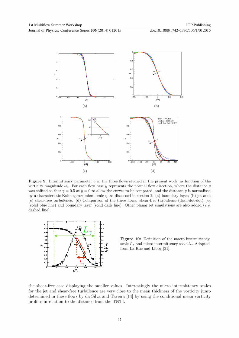
Figures 9(a), 9(b), and 9(c) show the intermittency factor for different values of the vorticitythreshold for the boundary layer, jet and shear-free turbulence, respectively. Because for eachvalue of ω0 the intermittency factor γ is centred at a different value of y, the curves were allshifted to have y = 0 whenever γ = 0.5, in order to allow the comparison between curves. Thenormal distance is normalised by the Kolmogorov micro-scale defined in section 2 for each flow.

The intermittency factor is quite insensitive to the vorticity magnitude, particularly for theshear-free turbulence case. The three cases are compared in figure 9(d) where one can see that γis very similar in the boundary layer and the jet, but definitively sharper in the shear-free case.

In order to quantify these differences we define a macro and a micro intermittency scales Lγand lγ , respectively. Since the intermittency factor is function of the normal distance, γ = γ (y),we define the coordinates corresponding to the start (ys) and end (ye) of the intermittency regionas γ (ys) = 1 and γ (ye) = 0 respectively. The macro intermittency scale is then defined as thespatial extent of the intermittence region in the flow,

Lγ = |ys − ye|. (8)

The micro intermittency scale lγ is defined as the scale associated with the maximum localderivative of the intermittency factor and thus represents the smallest length scale associatedwith the intermittency events,

lγ = |dγ/dy|−1max. (9)

The two scales are defined in figure 10 by adapting a figure from La Rue and Libby [31] displayingthe intermittency factor from the flow in the wake of a heated cylinder, and table 2 summarisesthe values obtained for the three flows analysed in this study. In agreement with the observationmade in figure 9(d) the spatial extent of the large and small scale intermittency events for theboundary layer and the jet have similar magnitudes, and are much bigger than for the shear-freecase. The micro intermittency scales display smaller values, but follow the same hierarchy, with


11

(a)

y/η

γ

200 100 0 100 2000

0.2

0.4

0.6

0.8

1

ω0

(b)

y/η

γ

100 0 100 2000

0.2

0.4

0.6

0.8

1

ω0

y/η5 0 5

0.35

0.5

0.65ω

0

(c)

y/d

a

-225 -150 -75 0 75 150 2250

0.2

0.4

0.6

0.8

1 Solid : PJChanDashed : PJkh120Dash Dot Dot : SFIIT

t0

(d)

Figure 9: Intermittency parameter γ in the three flows studied in the present work, as function of thevorticity magnitude ω0. For each flow case y represents the normal flow direction, where the distance ywas shifted so that γ = 0.5 at y = 0 to allow the curves to be compared, and the distance y is normalisedby a characteristic Kolmogorov micro-scale η, as discussed in section 2: (a) boundary layer; (b) jet and;(c) shear-free turbulence. (d) Comparison of the three flows: shear-free turbulence (dash-dot-dot), jet(solid blue line) and boundary layer (solid dark line). Other planar jet simulations are also added (e.g.dashed line).

Figure 10: Definition of the macro intermittencyscale Lγ and micro intermittency scale lγ . Adaptedfrom La Rue and Libby [31].

the shear-free case displaying the smaller values. Interestingly the micro intermittency scalesfor the jet and shear-free turbulence are very close to the mean thickness of the vorticity jumpdetermined in these flows by da Silva and Taveira [14] by using the conditional mean vorticityprofiles in relation to the distance from the TNTI.


12

Table 2: Macro intermittency scale Lγ and microintermittency scale lγ estimated for the three flowsanalysed in the present work.

Flow Lγ/η lγ/η

Boundary layer 155 20Turbulent jet 180 14Shear-free 70 5

yI

0 0.05 0.1 0.15 0.2 0.25 0.3 0.35 0.40

2

4

6

8

10

12

1

1

22

Figure 11: Sketch explaining the two methodsused to obtain the local values of δω. Method1: Distance between the TNTI (yi = 0) and thefirst ‘acceptable’ local vorticity maximum ωmax(dashed). Method 2: Distance between the first‘acceptable’ local maximum ωmax (dashed) and theprevious local minimum (solid)

6. Statistics of the local interface thickness δω in the planar turbulent jet.The mean interface thickness 〈δω〉 was analysed in turbulent planar jets and in shear-freeturbulence by da Silva and Taveira [14], for Reynolds numbers in 115 < Reλ < 160, whereit was defined by the length of the mean vorticity jump observed across the TNTI. In virtuallyall the flows assessed so far the conditional mean profile of ω exhibits a sharp jump at theTNTI and, after this jump, ω is roughly constant inside the turbulent region. Not surprisingly,da Silva and Taveira [14] observed that the large-scale eddy structure underneath the interfaceimposed 〈δω〉. However no information exists for the local TNTI thickness. This information isimportant in order to characterise the small-scale geometry of the interface and may be usefulto develop detailed models of its local dynamics. The thickness we use here can be seen as alength scale associated with the process needed for the flow to go from the irrotational to theturbulent region. This is not a ‘geometrical’ thickness, which does not seem to exist. Rather itis a thickness associated with the dynamics of the vorticity near the TNTI.

In order to characterise the local interface geometry a local thickness δω must be defined. Inthe present work two definitions were used based on the local conditional vorticity profiles asshown in figure 11. With ‘method 1’ the local thickness δω is defined as the distance from thelocation of the TNTI to the first ‘acceptable’ maximum, while in ‘method 2’, δω is defined asthe distance between this maximum and the nearest local minimum. The maximum vorticityobserved in the conditional (instantaneous) profiles is ωmax.

6.1. Fractions of δω and ωmax from the total number of samples of both quantitiesThe tables 3 and 4 compile information from the local (instantaneous) values of the local interfacethickness δω and maximum vorticity at the interface ωmax. The events are separated accordingto the vorticity magnitude ωmax and the size of the vorticity jump δω. Following Jimenez andWray [30] we separate the vorticity events between intense vorticity (ωmax > ωivs, where ωivsis the vorticity threshold that covers 1% of the total volume), weak (ωrms < ωmax < ωivs),and background vorticity (ωmax < ωrms). It has been shown that regions of intense vorticity inisotropic turbulence (intense vorticity structures - IVS) tend to be concentrated in thin vortextubes (‘worms’), and that very few vortices exist with radius smaller than 3η or greater than10η. We therefore separate the local TNTI thickness into incoherent (δω/η < 3), small scale(3 < δω/η < 10), and intermediate-large scale (δω/η > 10).

The values are slightly different using the two methods, but some results are consistent. Only


13

Table 3: Fraction of events contributing to the local TNTI thickness δω using ‘method 1’ (see textfor details). The events are separated according to the local vorticity magnitude into background, weakand intense events, and the local thickness is separated into δω/η > 3, 3 < δω/η < 10, and δω/η > 10,respectively.

Background Weak Intenseδω/η ωmax < ωrms ωrms < ωmax < ωivs ωmax > ωivs

Incoherent < 3 4.7% 1.2% < 0.1% 5.9%Small scale > 3 and < 10 34.4% 35.5% 3.5% 73.4%Intermediate-large scale > 10 6.9% 12.1% 1.5% 20.6%

Total 46.0% 12.1% 5.1% ≈ 100%

Table 4: As in table 3, using ‘method 2’ (see text for details).

Background Weak Intenseδω/η ωmax < ωrms ωrms < ωmax < ωivs ωmax > ωivs

Incoherent < 3 5.4% < 0.1% < 0.1% 5.5%Small scale > 3 and < 10 47.4% 10.5% 1.1% 60.0%Intermediate-large scale > 10 23.1% 10.8% 1.6% 45.5%

Total 75.9% 20.3% 2.7% ≈ 100%

approximately 5% of the weak vorticity events are contained in vorticity jumps smaller than 3η,which suggests that no structures smaller than IVS exist near the TNTI. This result is consistentwith da Silva et al. [15] where the tracking of the IVS near the TNTI was made, reachingsimilar conclusions. On the other hand most of the observed events are associated with smallscale thickness (3 < δω/η < 10) and weak and background vorticity. This is an interesting resultbecause the mean vorticity thickness for this simulation is slightly higher 〈δω〉 /η ∼ 16η ∼ λ.However very few of the events are associated with particularly strong vorticity magnitudes,again consistent with da Silva et al. [15]. This suggests that the TNTI is mostly ‘made up’ ofsmall-scale eddies but exhibiting vorticity magnitudes that are smaller than the IVS from thecore of the turbulent region. This also shows, as expected, that the vorticity magnitude at theTNTI is very small consisting in mostly background and some weak vorticity.

6.2. Probability density functions of local interface thicknessFigure 12(a) shows p.d.f.s of local interface thickness δω computed with the two methodsdescribed before. The p.d.f. shows that δω displays a large range of values with a peak aroundδω/η ≈ 5 − 6 which coincides with the mean radius of the IVS, while the mean thickness -around δω/η ≈ 16 in this case - is not far off, but results from averaging a large range of possiblevalues, and does not arise ‘naturally’ from the data. Arguably the scatter in the results willbe even higher at high Reynolds numbers, where no large-scale eddy is likely to survive thebackground field of fluctuating strain, implying that the mean value of δω will probably tendmore to 〈δω〉 ∼ η than to 〈δω〉 ∼ λ as is the case here.

Figure 12(b) shows the joint p.d.f. of the local vorticity maximum ωmax and of the TNTIthickness δω. It is difficult to observe a correlation between the two quantities, which agrees withthe results displayed in tables 3 and 4, i.e., events of low/high vorticity are not associated witheither low/high local thickness, suggesting that the TNTI is defined by a low vorticity magnitudethreshold, which is not from the core but rather from the periphery of the flow vortices.


14

δω/η

pd

f(δ

ω/η

)

0 15 30 45 60 75

104

103

102

101

δω/η

pd

f(δ

ω/η

)

0 5 10 15 2010

3

102

101

(a)

δω/η

ω*

0 5 10 15 20 250

3

6

9

(b)

Figure 12: (a) P.d.f.s of local thickness δω from the instantaneous vorticity conditional profiles forthe planar jet using ‘method 1’ (green) and ‘method 2’; (b) Joint p.d.f.s of vorticity magnitudesω∗ = ωmax/ωrms and local thickness δω from the instantaneous vorticity conditional profiles using‘method 1’.

7. Low vorticity regions embedded in turbulent flow, and their role inentrainment.One resilient discussion about the mechanism of entrainment is how the irrotational fluid actuallyacquires vorticity. Two different possibilities can be found in the literature: one in which vorticityis transmitted by direct shearing contact with the turbulent eddies across the turbulent/non-turbulent interface, and a second in which some coherent structure encloses the irrotational flowforming pockets or bubbles (defined as regions of low vorticity completely surrounded by fluid athigher vorticity) that are later given vorticity. The two mechanisms are usually called nibblingand engulfing respectively. This distinction is ambiguous. A pocket can be considered a signof nibbling and engulfment. To avoid this ambiguity, engulfment will be considered only if thezone with low vorticity is completely surrounded, and becomes isolated.

Nibbling is inherently small-scale, because direct shearing contact can only happen by effectof viscosity. Engulfment, however, can happen at many different scales. Low-vorticity bubblesare as large as the coherent structure that encloses them, which includes almost any scalepresent in the flow. It is also a purely three-dimensional definition, and cannot be appliedif vorticity is measured on a plane, or the data set provides only one vorticity component.Fortunately, the data available for this study fulfils the previous requirements, and algorithmsfor fast identification of isolated structures (commonly called labeling) are presently available.

Figure 13 is the result of labelling two different flows with two different thresholds, belowand above the proposed value to detect the turbulent/non-turbulent interface for the jetω0 = 0.1ωrms. A cut of the contour of every structure detected is marked with a solid line.It can be seen in figure 13b, that the flow of the jet sparsely marked with many low-vorticityregions. At this low threshold, the question arises whether these regions are a product of theinteraction between the turbulent eddies and the free stream, or a feature of any turbulentflow. To find an answer to the previous question, the planar jet is compared to a homogeneousand isotropic turbulence (HIT) box at a similar Reynolds number (Reλ = 168)[30], where theisolated bubbles have been detected using the same technique and a comparable threshold. Giventhat HIT contains no such thing as a turbulent/non-turbulent interface, any obvious differencebetween the two flows may be due to the interaction between the turbulent eddies and the freestream.

Two comparisons are presented in figure 13, one at a lower threshold (figure 13 a, and b),


15

Figure 13: Cuts of the boundaries of low-vorticity bubbles at different thresholds for jets and HIT.The lengths are represented in the Kolmogorov units. Given that the outer stream is identified as alow-vorticity spot, the interface detection can always be seen in the case of the jet. In the case of thehigher threshold in homogeneous turbulence, there is a single low-vorticity region that covers a relevantpart of the volume, and is also detected as a spot.

and a second one at a higher threshold (figure 13 c, and d). If one ignores that the bubbles inthe planar jet are confined to the fully turbulent flow, the shape and density of bubbles is prettysimilar. But this observation, based purely on perception, is not quantitative.

To add more consistency to the previous comparison, the probability density of the volumesof these bubbles is computed at four different thresholds, for the planar jet and the HIT box.The context of those thresholds is clarified by the figure 14, where every threshold is markedwith a vertical dashed line. The values cover a range of values of half an order of magnitude,close to the one chosen to detect the interface. The same unit for vorticity is used in both flowsgiven that, according to figure 14, ωrms makes the two flows comparable in the explored range.

The p.d.f of the size of the low-vorticity bubbles, expressed as the cubic root of their volume,is presented in figures 15(a-d). It follows a power-law distribution with an exponent of −3,represented in figure 15(a-d) as a dashed line, which argues for a self-similar origin without acharacteristic length scale.

Interestingly, figure 15 shows that the HIT and planar jets follow a similar power law forbubble size, strongly suggesting that their formation is not heavily affected by the presence ofirrotational flow in the case of the jet.

This result questions the idea that engulfment exists in the form of bubbles of free-streamirrotational fluid trapped by large coherent structures. According to these results, bubbles of


16

10-5 10-4 10-3 10-2 10-1 100 101

ω/ωrms

10-6

10-5

10-4

10-3

10-2

10-1

100

101

PDF

Jet

HIT

Figure 14: Probability density of vorticity mag-nitude for planar jets (solid line) and homogeneousisotropic turbulence (circles) using the r.m.s. of vor-ticity magnitude as unit. The bimodal behaviourin jets is described in figure 3. The distribution ofvorticity in the peak corresponding to the fully tur-bulent fluid is similar, and confirms that ωrms is asuitable unit to compare HIT and planar jets. Thefour vertical dashed lines correspond to the thresh-olds used in the results presented in figure 15

100 101 102 10310-4

10-3

10-2

10-1

100

101

PDF

(a)ω/ωrms=0.08

Jet

HIT

100 101 102 10310-4

10-3

10-2

10-1

100

101 (b)ω/ωrms=0.14

100 101 102 103

3√V/η

10-4

10-3

10-2

10-1

100

101

PDF

(c)ω/ωrms=0.23

100 101 102 103

3√V/η

10-4

10-3

10-2

10-1

100

101 (d)ω/ωrms=0.40

Figure 15: Probability density of thecharacteristic length of the low-vorticitybubbles for homogeneous isotropic tur-bulence (circles) and planar jets (solidlines). The thresholds are represented infigure 14 as dashed lines. The straightlines correspond to the exponent for scaleinvariance ( 3

√V /η)−3.

low vorticity are found in the fully turbulent fluid, but they are very similar to the bubblesfound in internal flows, where the mentioned mechanism cannot occur.

8. ConclusionsDirect numerical simulations of a boundary layer, a planar jet and shear-free turbulence atReynolds numbers slightly higher than Reλ = 100 are used to compare the characteristics of theTNTI in different flows.

A prerequisite to compare the three TNTI is the determination of the location of the TNTIin each flow. In the present work, the technique used for this detection relies on computing thevolume of turbulent region as a function of the vorticity magnitude. For the three flows analysedhere, the volume of the turbulence region exhibits a characteristic change with the vorticitymagnitude, displaying an inflection point. The vorticity magnitude threshold corresponding tothis inflection point is used to define the TNTI. It is shown that this method is equivalent towell-known experimental methods used to detect scalar interfaces.

Vorticity maps displaying vorticity p.d.f.s as functions of a distance along the mostinhomogeneous direction of the flow are computed for the three flows and show distinctivefeatures in each of them. Specifically, the range of vorticity scales displayed in the boundarylayer is larger than in the other flows, and the change of ‘shape’ across the TNTI is less dramatic.The vorticity maps are normalised, and the one for the boundary layer is rescaled to allow acomparison which determines a vorticity threshold used to compared the three TNTIs.


17

Visualisations of the TNTIs for boundary layers and jets are compared, and show that thestatistics of the interface height are not random and the observed differences suggest the imprintof the different underlying large-scale vortices in the two flows.

The intermittency parameters were computed for the three TNTIs, and length scales weredefined. A large scale associated with the maximum extent of the intermittency region and asmall scale associated with the strongest gradient across this region. In the present case the large-scale intermittency regions for boundary layers and jets were comparable and significantly largerthan in the shear-free case. Interestingly the small intermittency scale is similar to the computedvorticity thickness (or jump) observed in the jet and shear-free case, suggesting another methodto quantify the so called TNTI thickness (identified) as the turbulent sub-layer.

Finally, an analysis is made of the irrotational bubbles trapped inside the turbulent region,which are typically associated with ‘engulfing’ events in several flows. The analysis shows that,contrary to the classical view, the spots of low vorticity found inside the jet follow a power law,which is exactly the same observed in isotropic turbulence, where engulfing events do not exist.This suggests that the vast majority of these regions are not associated with engulfment.

AcknowledgmentsThis work was performed in part during the first Multiflow summer school at Madrid, andpartially funded by the European Research Council.

References[1] Corrsin S and Kistler A L 1955 Free-stream Boundaries of Turbulent Flows Tech. Rep. TN-1244 NACA[2] Townsend A A 1966 The mechanism of entrainment in free turbulent flows J. Fluid Mech. 26 689–715[3] Mathew J and Basu A 2002 Some characteristics of entrainment at a cylindrical turbulent boundary Phys.

Fluids 14 2065–72[4] Westerweel J, Fukushima C, Pedersen J M and Hunt J C R 2005 Mechanics of the turbulent-nonturbulent

interface of a jet Phys. Rev. Lett. 95 174501[5] Westerweel J, Fukushima C, Pedersen J M and Hunt J C R 2009 Momentum and scalar transport at the

turbulent/non-turbulent interface of a jet J. Fluid Mech. 631 199–230[6] Holzner M, Liberzon A, Nikitin N, Luthi B, Kinzelbach W and Tsinober A 2008 A Lagrangian investigation

of the small-scale features of turbulent entrainment through particle tracking and direct numerical simulationJ. Fluid Mech. 598 465–75

[7] da Silva C B and Pereira J C F 2008 Invariants of the velocity-gradient, rate-of-strain, and rate-of-rotationtensors across the turbulent/nonturbulent interface in jets Phys. Fluids 20 055101

[8] Taveira R R and da Silva C B 2013 Kinetic energy budgets near the turbulent/nonturbulent interface injets Phys. Fluids 25 015114

[9] Taveira R R, Diogo J S, Lopes D C and da Silva C B 2013 Lagrangian statistics across the turbulent-nonturbulent interface in a turbulent plane jet Phys. Rev. E 88 043001

[10] Townsend A A 1976 The Structure of Turbulent Shear Flow (Cambridge: Cambridge University Press)[11] Gampert M, Narayanaswamy V, Schaefer P and Peters N 2013 Conditional statistics of the turbulent/non-

turbulent interface in a jet flow J. Fluid Mech. 731 615–38[12] Wolf M, Luthi B, Holzner M, Krug D, Kinzelbach W and Tsinober A 2013 Investigations on the local

entrainment velocity in a turbulent jet Phy. Fluids 24 105110[13] da Silva C B and dos Reis R J N 2011 The role of coherent vortices near the turbulent/non-turbulent

interface in a planar jet Phil. Trans. R. Soc. A 369 738–53[14] da Silva C B and Taveira R R 2010 The thickness of the turbulent/nonturbulent interface is equal to the

radius of the large vorticity structures near the edge of the shear layer Phys. Fluids 22 121702[15] da Silva C B, dos Reis R J N and Pereira J C F 2011 The intense vorticity structures near the turbulent/non-

turbulent interface in a jet J. Fluid Mech. 685 165–90[16] Mandelbrot B B 1982 The Fractal Geometry of Nature (New York: W. H. Freeman)[17] Sreenivasan K R 1991 Fractals and multifractals in fluid turbulence Ann. Rev. Fluid Mech. 23 539–600[18] Frederiksen R D, Dahm W J A and Dowling D R 1997 Experimental assessment of fractal scale similarity

in turbulent flows. Part 3. Multifractal scaling J. Fluid Mech. 338 127–55[19] Catrakis H J, Aguirre R C, Ruiz-Plancarte J and Thayne R D 2002 Shape complexity of whole-field three-

dimensional spacetime fluid interfaces in turbulence Phys. Fluids 14 3891


18

[20] de Silva C M, Philip J, Chauhan K, Meneveau C and Marusic I 2013 Multiscale geometry and scaling of theturbulent-nonturbulent interface in high Reynolds number boundary layers Phys. Rev. Lett. 111 044501

[21] Westerweel J, Hofmann T, Fukushima C and Hunt J C R 2002 The turbulent/non-turbulent interface atthe outer boundary of a self-similar turbulent jet Exp. Fluids 33 873–78

[22] Simens M P, Jimenez J, Hoyas S and Mizuno Y 2009 A high-resolution code for turbulent boundary layersJ. Comput. Phys. 228 4218–31

[23] Borrell G, Sillero J A and Jimenez J 2013 A code for direct numerical simulation of turbulent boundarylayers at high Reynolds numbers in BG/P supercomputers Comput. Fluids 80 37–43

[24] Sillero J A, Jimenez J and Moser R D 2013 One point statistics for turbulent wall-bounded flows at Reynoldsnumbers up to δ+ = 2000 Phys. Fluids 25, 105102

[25] Perot B and Moin P 1995 Shear-free turbulent boundary layers. Part 1. Physical insights into near-wallturbulence J. Fluid Mech. 295 199–227

[26] Teixeira M and da Silva C B 2012 Turbulence dynamics near a turbulent/non-turbulent interface J. FluidMech. 695 257–287

[27] Bisset D K, Hunt J C R and Rogers M M 2002 The turbulent/non-turbulent interface bounding a far wakeJ. Fluid Mech. 451 383–410

[28] Prasad R and Sreenivasan K R 1989 Scalar interfaces in digital images of turbulent flows Exp. Fluids 7259–264

[29] Lozano-Duran A and Jimenez J 2014 Effect of the computational domain in direct simulations of turbulentchannels up to Reτ = 4200 Phys. Fluids 26 011702

[30] Jimenez J, Wray A A, Saffman P G and Rogallo R S 1993 The structure of intense vorticity in isotropicturbulence J. Fluid Mech. 255 65–90

[31] Rue J C L and Libby P A 1976 Statistical properties of the interface in the turbulent wake of a heatedcylinder Phys. Fluids 19 1864–75


19

Characteristics of the turbulent/nonturbulent interface in boundary layers, jets and shear-free...

Documents

Transcript of Characteristics of the turbulent/nonturbulent interface in boundary layers, jets and shear-free...