arX

iv:0

904.

0557

v2 [

phys

ics.

flu-

dyn]

17

Jul 2

009

Growth rate of Rayleigh-Taylor turbulent mixing layers

from first principles

Olivier Poujade∗ and Mathieu Peybernes

CEA, DAM, DIF, F-91297 Arpajon, France

(Dated: July 17, 2009)

Abstract

For years, astrophysicists, plasma fusion and fluid physicists have puzzled over Rayleigh-Taylor

turbulent mixing layers. In particular, strong discrepancies in the growth rates have been observed

between experiments and numerical simulations. Although two phenomenological mechanisms

(mode-coupling and mode-competition) have brought some insight on these differences, convincing

theoretical arguments are missing to explain the observed values. In this paper, we provide an

analytical expression of the growth rate derived from first principles. It is compatible with both

mechanisms and is valide for a self-similar, low Atwood Rayleigh-Taylor turbulent mixing subjected

to a constant or time-varying acceleration. The key step in this work is the introduction of foliated

averages and foliated turbulent spectra highlighted in our three dimensional numerical simulations.

We show that the exact value of the Rayleigh-Taylor growth rate not only depends upon the

acceleration history but is also bound to the power-law exponent of the foliated spectra at large

scales.

PACS numbers: 52.35.Py, 47.20.Bp, 47.27.eb, 47.27.te

1

I. INTRODUCTION

If allowed to evolve long enough, the Reynolds number of a Rayleigh-Taylor (RT) flow

[1, 2] increases and the mixing eventually becomes fully turbulent [3, 4]. Then, at late time,

the width of the mixing layer grows according to

L(t) = αp A g(t) t2 (1)

when the gravitational field history [5] is of the form g(t) ∝ tp. The Atwood number A

quantifies the density contrast of the initially pure fluids and is tied to the acceleration in

any buoyant flow. From a purely theoretical point of view, the RT growth rate coefficient

αp should be universal if the late stage of the evolution of the mixing zone is self similar and

should only depend upon the exponent p of the gravitational field history. However, even

today, the value of ”alpha” (α), which is the name given by the ”alpha-group collaboration”

[3] to αp/2 when p = 0 (constant acceleration), is still a subject of controversy.

For years, the discrepancy between its value inferred from numerical simulations [3, 4, 6, 7]

(initialised with small wave lengths), scattered around 0.05, and its experimental values

[8, 9, 10, 11], twice as large, has thrown doubt on its universality. Not long ago, the heuristic

mode-competition mechanism [12, 13] put an end to this paradox: adding a small amount

of modes of large wave length to the perturbation of the initial interface helps increase the

value of α and reconciles numerical simulations with laboratory experiments. But, it is

also instrumental in demonstrating that the initial conditions in any laboratory experiments

do feature these modes of large wave length triggered by external causes like vibrations

and residual motions. Flows of interest (geophysics, atmospheric, astrophysics [14, 15]), to

a large extent, are not confined to a laboratory. Orders of magnitude may separate the

length scales of the interface perturbation with the geometric size of the flow. This is why,

the mode-coupling mechanism, initiated with small wave length modes, is thought to be

realised in astrophysical mixing [4] and other natural flows.

Here, in order to find the theoretical value of the growth rate (αp), we have adopted a

point of view which has been used in the study of homogeneous turbulence (HT) for almost

half a century but never investigated in RT turbulent mixing. The ”large-scale structure of

homogeneous turbulence” [16, 17] has been studied to understand the conjectured persistence

of big eddies and the decay rate of various physical quantities in turbulent flows. At large

scales, the turbulent kinetic energy density spectrum behaves as E(k) ∝ ks where the value

2

of s depends on the initialisation of freely decaying HT in a way which is still unclear

[18, 19, 20, 21, 22]. Bulk quantities of such flows, like turbulent kinetic energy, vary as

power-laws at late time and their exponents appear solely related to the value of s [23].

That underlines the fact that large scale spectra have a strong influence on the behaviour

of the overall flow. The theoretical study of freely decaying HT is made difficult by the

fact that large scales are driven by non linear effect (triadic interaction). In contrast, the

RT turbulence, although anisotropic, displays a significant difference with freely decaying

HT. When plunged in a gravitational field, density fluctuations produce motion through

buoyancy. This production mechanism affects all scales [24], even the largest, and produces

turbulent kinetic energy at all times. It overcomes non linear transfer mechanism at large

scales making the theoretical study of RT turbulence much easier.

Here we demonstrate that it is possible to display an exact formula for αp which depends

upon p, the exponent of the acceleration history, and s, the power-law exponent at large

scales of foliated spectra that rise up naturally, along with foliated average, from the theo-

retical developments hereafter. This foliation procedure is introduced for the first time in

turbulent mixing theory because, among other interesting features, it allows to cancel out

the formal effect of pressure in the equations, while keeping its physical effect on the whole

mixing zone, making theoretical calculations amenable.

II. TRANSVERSE AVERAGE

A RT mixing occurs whenever two fluids of different density, initially separated by a sharp

interface, are subjected to a gravitational field directed from the heavier (density ρh) to the

lighter (density ρl) and when the initial interface is slightly distorted by a perturbation

whose spectrum contains modes with sufficiently large wave lengths to overcome viscous

effects at the onset. Such a flow, with two incompressible fluids in the low Atwood limit

A = (ρh−ρl)/(ρh +ρl) ≪ 1 (Boussinesq approximation), is governed [25] by a concentration

equation (2), the Navier Stokes equation supplemented with a buoyant source term (3), and

3

the incompressibility constraint (4)

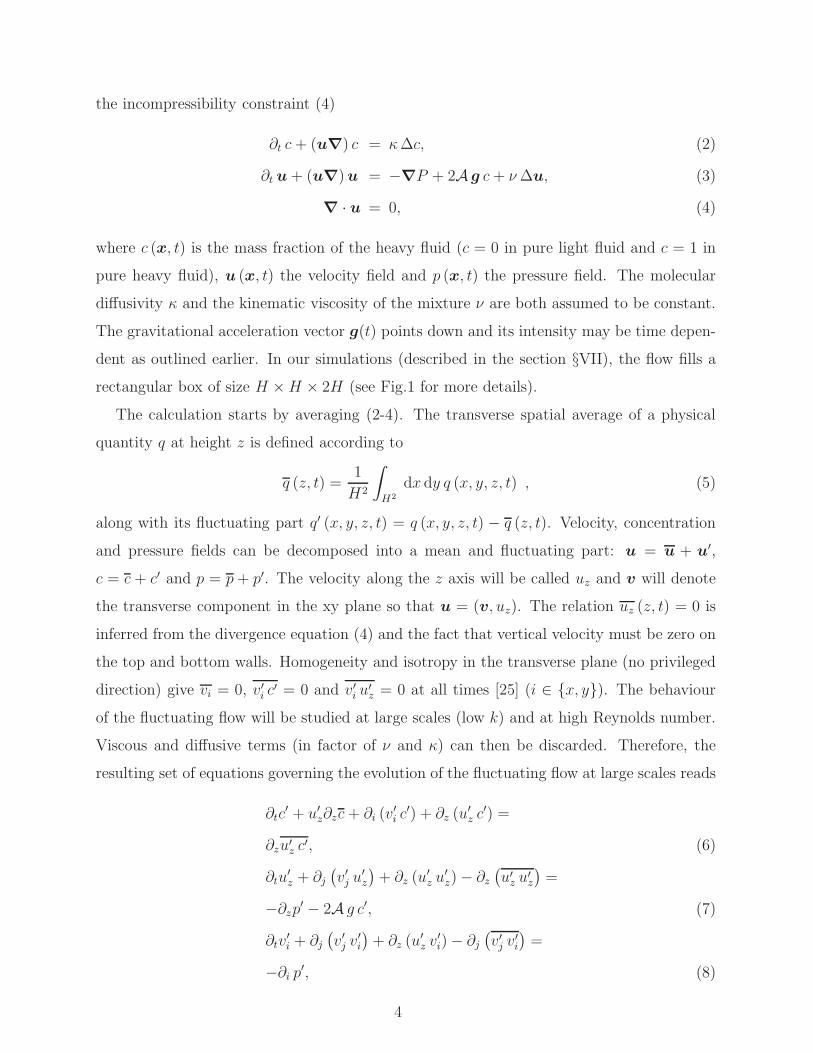
∂t c + (u∇) c = κ ∆c, (2)

∂t u + (u∇) u = −∇P + 2A g c + ν ∆u, (3)

∇ · u = 0, (4)

where c (x, t) is the mass fraction of the heavy fluid (c = 0 in pure light fluid and c = 1 in

pure heavy fluid), u (x, t) the velocity field and p (x, t) the pressure field. The molecular

diffusivity κ and the kinematic viscosity of the mixture ν are both assumed to be constant.

The gravitational acceleration vector g(t) points down and its intensity may be time depen-

dent as outlined earlier. In our simulations (described in the section §VII), the flow fills a

rectangular box of size H × H × 2H (see Fig.1 for more details).

The calculation starts by averaging (2-4). The transverse spatial average of a physical

quantity q at height z is defined according to

q (z, t) =1

H2

∫

H2

dx dy q (x, y, z, t) , (5)

along with its fluctuating part q′ (x, y, z, t) = q (x, y, z, t) − q (z, t). Velocity, concentration

and pressure fields can be decomposed into a mean and fluctuating part: u = u + u′,

c = c + c′ and p = p + p′. The velocity along the z axis will be called uz and v will denote

the transverse component in the xy plane so that u = (v, uz). The relation uz (z, t) = 0 is

inferred from the divergence equation (4) and the fact that vertical velocity must be zero on

the top and bottom walls. Homogeneity and isotropy in the transverse plane (no privileged

direction) give vi = 0, v′i c

′ = 0 and v′i u

′z = 0 at all times [25] (i ∈ x, y). The behaviour

of the fluctuating flow will be studied at large scales (low k) and at high Reynolds number.

Viscous and diffusive terms (in factor of ν and κ) can then be discarded. Therefore, the

resulting set of equations governing the evolution of the fluctuating flow at large scales reads

∂tc′ + u′

z∂zc + ∂i (v′

i c′) + ∂z (u′

z c′) =

∂zu′z c′, (6)

∂tu′

z + ∂j

(v′

j u′

z

)+ ∂z (u′

z u′

z) − ∂z

(u′

z u′z

)=

−∂zp′ − 2A g c′, (7)

∂tv′

i + ∂j

(v′

j v′

i

)+ ∂z (u′

z v′

i) − ∂j

(v′

j v′i

)=

−∂i p′, (8)

4

where Einstein summation convention is used on the repeated indices i and j ∈ x, y.

III. FOLIATED AVERAGE

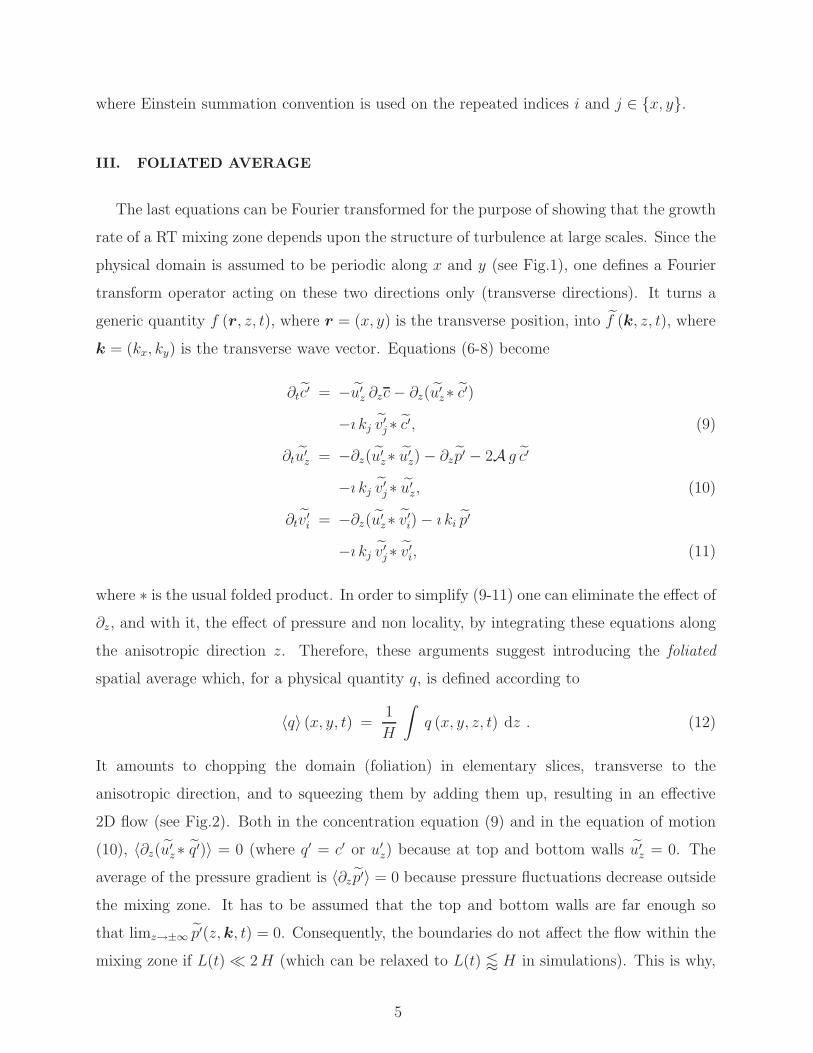
The last equations can be Fourier transformed for the purpose of showing that the growth

rate of a RT mixing zone depends upon the structure of turbulence at large scales. Since the

physical domain is assumed to be periodic along x and y (see Fig.1), one defines a Fourier

transform operator acting on these two directions only (transverse directions). It turns a

generic quantity f (r, z, t), where r = (x, y) is the transverse position, into f (k, z, t), where

k = (kx, ky) is the transverse wave vector. Equations (6-8) become

∂tc′ = −u′z ∂zc − ∂z(u′

z∗ c′)

−ı kj v′j∗ c′, (9)

∂tu′z = −∂z(u′

z∗ u′z) − ∂zp′ − 2A g c′

−ı kj v′j∗ u′

z, (10)

∂tv′i = −∂z(u′

z∗ v′i) − ı ki p′

−ı kj v′j∗ v′

i, (11)

where ∗ is the usual folded product. In order to simplify (9-11) one can eliminate the effect of

∂z, and with it, the effect of pressure and non locality, by integrating these equations along

the anisotropic direction z. Therefore, these arguments suggest introducing the foliated

spatial average which, for a physical quantity q, is defined according to

〈q〉 (x, y, t) =1

H

∫q (x, y, z, t) dz . (12)

It amounts to chopping the domain (foliation) in elementary slices, transverse to the

anisotropic direction, and to squeezing them by adding them up, resulting in an effective

2D flow (see Fig.2). Both in the concentration equation (9) and in the equation of motion

(10), 〈∂z(u′z∗ q′)〉 = 0 (where q′ = c′ or u′

z) because at top and bottom walls u′z = 0. The

average of the pressure gradient is 〈∂z p′〉 = 0 because pressure fluctuations decrease outside

the mixing zone. It has to be assumed that the top and bottom walls are far enough so

that limz→±∞ p′(z, k, t) = 0. Consequently, the boundaries do not affect the flow within the

mixing zone if L(t) ≪ 2 H (which can be relaxed to L(t) / H in simulations). This is why,

5

the resulting concentration equation and equation of motion after foliated average are

∂t〈c′〉 = −〈u′z ∂zc 〉 − ı kj 〈v′

j∗ c′〉 , (13)

∂t〈u′z〉 = −2A g 〈c′〉 − ı kj 〈v′

j∗ u′z〉 . (14)

In eq.(13), the term 〈u′z ∂zc 〉 can be simplified because the profile of c(z, t) is a straight line

(constant slope), from 0 to 1, from one edge of the mixing zone to the other, at small Atwood

number. This is corroborated experimentally [10, 11] and numerically, in our simulations

(A = 0.1), to within statistical fluctuations due, at a given height z, to the finite number

N(t) ≈ H2/ℓ(t)2 of eddies in the transverse plane of area H2. The integral length scale ℓ(t),

i.e. the diameter of a typical eddy, varies like L(t) ∝ tp+2 in the self-similar regime. These

statistical fluctuations become negligible in the limit H → +∞ since their rms amplitude is

of the order 1/√

N(t) ≈ ℓ(t)/H . In this limit, the derivative ∂zc is then uniform within the

mixing zone. Thus, the theoretical development suggests defining L such that ∂zc = 1/L(t)

which can be brought close to another definition of the width at low Atwood number (see

the end of §VII). Therefore, it is possible to write 〈u′z ∂zc 〉 ≈ 〈u′

z〉 ∂zc = 〈u′z〉/L(t). As

a consequence, (i) at large scale (k ≪ 2π/ℓ(t)), (ii) at low Atwood (iii) at high Reynolds

number and (iv) in the limit H → +∞ (i.e. L(t) ≪ H), the evolution of foliated second

moments can be derived. From eqs.(13-14), straightforward algebraic manipulations provide

∂t(〈c′〉〈c′〉∗) = −

2 Re[〈u′z〉〈c

′〉∗]

L(t)

−kj ξcj , (15)

∂t(〈u′z〉〈u

′z〉

∗) = −4A g Re[〈u′z〉〈c

′〉∗]

−kj ξzj , (16)

∂t(Re[〈u′z〉〈c

′〉∗]) = −2A g 〈c′〉〈c′〉∗ −〈u′

z〉〈u′z〉

∗

L(t)

−kj ξczj , (17)

where ξcj = 2 Re[ı〈v′

j ∗ c′〉〈c′〉∗], ξzj = 2 Re[ı〈v′

j ∗ u′z〉〈u

′z〉

∗] and ξczj = Re[ı〈v′

j ∗ u′z〉〈c

′〉∗] +

Im[ı〈v′j ∗ c′〉〈u′

z〉∗] cancelled out when ensemble averaged.

IV. ENSEMBLE AVERAGED FOLIATED SPECTRA

Let us note q the ensemble average of a generic quantity q. Because of isotropy in the

transverse direction in the self-similar fully turbulent regime, ξcj(k, t) = 0, ξz

j (k, t) = 0 and

6

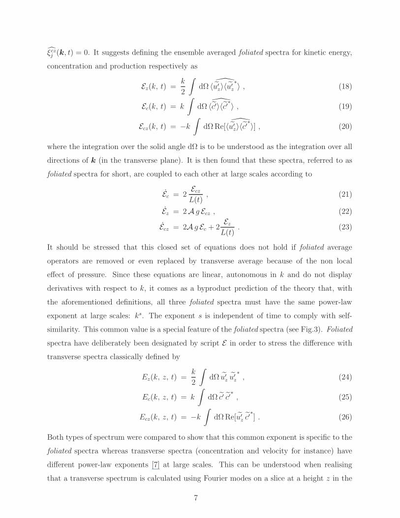
ξczj (k, t) = 0. It suggests defining the ensemble averaged foliated spectra for kinetic energy,

concentration and production respectively as

Ez(k, t) =k

2

∫dΩ

〈u′

z〉〈u′z

∗

〉 , (18)

Ec(k, t) = k

∫dΩ

〈c′〉〈c′

∗

〉 , (19)

Ecz(k, t) = −k

∫dΩ Re[

〈u′

z〉〈c′∗

〉] , (20)

where the integration over the solid angle dΩ is to be understood as the integration over all

directions of k (in the transverse plane). It is then found that these spectra, referred to as

foliated spectra for short, are coupled to each other at large scales according to

Ec = 2Ecz

L(t), (21)

Ez = 2A g Ecz , (22)

Ecz = 2A g Ec + 2Ez

L(t). (23)

It should be stressed that this closed set of equations does not hold if foliated average

operators are removed or even replaced by transverse average because of the non local

effect of pressure. Since these equations are linear, autonomous in k and do not display

derivatives with respect to k, it comes as a byproduct prediction of the theory that, with

the aforementioned definitions, all three foliated spectra must have the same power-law

exponent at large scales: ks. The exponent s is independent of time to comply with self-

similarity. This common value is a special feature of the foliated spectra (see Fig.3). Foliated

spectra have deliberately been designated by script E in order to stress the difference with

transverse spectra classically defined by

Ez(k, z, t) =k

2

∫dΩ u′

z u′z

∗

, (24)

Ec(k, z, t) = k

∫dΩ c′ c′

∗

, (25)

Ecz(k, z, t) = −k

∫dΩ Re[u′

z c′∗

] . (26)

Both types of spectrum were compared to show that this common exponent is specific to the

foliated spectra whereas transverse spectra (concentration and velocity for instance) have

different power-law exponents [7] at large scales. This can be understood when realising

that a transverse spectrum is calculated using Fourier modes on a slice at a height z in the

7

middle of the mixing zone. A foliated spectrum, on the other hand, uses the sum along z of

all these modes. The resulting spectrum is radically different and benefits from interferences

between modes at different heights.

V. GROWTH RATE FORMULA

For self-similarity to hold, the late time behaviour of the foliated spectra must be

Ez(k, t) = E0z ks tez , (27)

Ec(k, t) = E0c ks tec , (28)

Ecz(k, t) = E0cz ks tecz , (29)

at low k where E0c , E0

z and E0cz are constants independent from k and t. In addition, the

exponent of k in each of this averaged spectrum (s) and the time exponents (ec, ez, ecz)

must be constant in time. When replacing these expressions with A g(t) = A gp tp and

L(t) = αp A gp tp+2 in eqs. (21-23) one gets the following relations

ez = ec + 2(p + 1) , (30)

ecz = ec + (p + 1) , (31)

E0z = (αp (A gp)

2 ec/ez) E0c , (32)

E0cz = (αp A gp ec/2) E0

c , (33)

αp =8

ez ec

, (34)

which are not modelled but come straight from first principles. Using Eqs.(27-29) and

eqs.(30-34), a non trivial exact result can be deduced: E2cz(k, t)/ (2 Ez(k, t)Ec(k, t)) = 1

valid at large scale (see Fig.4).

A fundamental feature of concentration is that its fluctuation variance, c′c′ tends to a

constant in the self-similar regime because concentration is a physical quantity bounded

between 0 and 1. It cannot go to zero for that would mean the mixing tends to be heteroge-

neous in the middle of the mixing zone, thereby going against the fact that at all times any

side of the mixing zone must be supplied with pure fluid from the other side. The mixed-

fluid-supplying-channels have been highlighted in Fig.1 and Fig.2. This is exemplified by

numerical simulations and experiments reporting molecular mixing rates ranging from 0.7

to 0.8 [3, 4, 10, 25].

8

The question now is: how about 〈c′〉〈c′〉? A very simple argument can be given:

the discretized foliated average 〈c′〉 = dz/H∑H/dz

i=−H/dz c′i can be approximated by 〈c′〉 ≈

dz/H∑L(t)/dz

i=−L(t)/dz c′i since c′ is only non zero within the mixing zone. That is why, 〈c′〉〈c′〉 ≈

dz2/H2∑L(t)/dz

i=−L(t)/dz

∑L(t)/dzj=−L(t)/dz c′ic

′j and 〈c′〉〈c′〉 ≈ dz2/H2

∑L(t)/dzi=−L(t)/dz

∑L(t)/dzj=−L(t)/dz c2

0 δij if

we say c′c′ = c20 in the self similar regime as described in the previous paragraph. Therefore,

〈c′〉〈c′〉 ≈ dz2/H2∑L(t)/dz

i=−L(t)/dz c20 = dz/H2 L(t) c2

0. As a result 〈c′〉〈c′〉 must grow like L(t)

(corroborated by our numerical simulations).

Therefore, since 〈c′〉〈c′〉 =∫ +∞

0dk Ec(k, t) varies as

∫ 2π/ℓ(t)∝ t−p−2

0dk Ec(k, t) ∝

tec−(p+2)(s+1) and must evolve as L(t) ∝ tp+2, the value of ec is bound to be (p+2)(s+2) and,

by inference, the time exponents ez = (p+2)(s+2)+2(p+1) and ecz = (p+2)(s+2)+(p+1).

Therefore, the value of the Rayleigh-Taylor growth rate for the turbulent mixing zone width,

αp, is shown to depend upon p, which is the acceleration exponent, and s, the foliated spec-

trum power-law exponent at large scales, according to

αp(s) =8

(p + 2)(s + 2)(p(s + 4) + 2(s + 3)). (35)

This expression does not depend on gp as expected and confirmed in our simulations.

The demonstration leading to this formula did not provide any arguments against the

idea of an s varying with p. However, growth rates, at various values of p given by our

simulations in conjunction with those provided in [26], were fitted to the theoretical formula

and a remarkable collapse of the data was found for s = 4.0±0.1 assuming s was independent

of p (see Fig.5). It is possible to check this result by using an other obvious method: direct

inspection of the foliated spectra. The power-law at large scales of foliated spectra was

checked on every simulation (p = 0, 1, 2 and 3) and was found to be compatible with

s = 4. The formula (35) is therefore a predictive formula: it gives the value of αp knowing

p (a controled parameter) and s or, the other way around, it gives s knowing p and αp.

Our theory did not provide a value for s for it certainly depends upon the way the mixing

flow reaches the self-similar regime. In order to find its value, the theory would have to

cope with the transition regime to make the connexion with the linear growth of the initial

conditions (s = 4 seems to be compatible with annular spectrum initial conditions). It

must be emphasized that the exact result (35) is a proof that, in the self-similar regime,

the growth of the mixing zone only depends upon the structure of turbulence at large scales

(appart from p, it depends on s only).

9

VI. IMPLICATIONS

Obviously, the formula for αp carries information on the dynamics of the mixing zone

width. Not so obvious is the fact that it also provides information on the way this dynamic

affects the mixing at large scale. If it is assumed that the late time evolution of the mixing

zone width does not depend upon initial conditions - which may be true when the charac-

teristic length scale of the initial perturbations is much smaller than that of the physical

domain H - it is reasonable to admit that it must depend on L(t) (and its derivatives) and

g(t) which are the only control parameters left in the problem. From this assumption, basis

of the buoyancy-drag approach [8, 27], it is possible to build a simple evolution equation,

L(t) = Cb A g(t) L(t) − Cd L2(t)/L(t) , (36)

which depends on two adjustable constants. The constant Cb quantifies buoyancy related to

the mixing since Cb A can be seen as an effective Atwood number: the fluids are not pure,

with density ρl and ρh, in the mixing zone but they are partly mixed with intermediate

densities and the smaller Cb, the smaller the effective Atwood number, the stronger the

mixing. The constant Cd quantifies drag, i.e. the exchange of momentum between raising

and falling mixed-fluids structures. This phenomenological approach does not by itself

provide any relation between these two adjustable constants. However, replacing the self-

similar values (1) of L and g in (36) allows to recover the exact formula (35) if and only

if Cb = 4/(s + 2) and Cd = (s + 2)/2, which yields Cb = 2/Cd. This correspondence

between the simple model and the exact result demonstrate the little importance of small

scale as opposed to large scale in the bulk dynamics of the mixing. Furthermore, it enables

to understand the influence of s on ”intuitive” physical mechanisms like buoyancy, through

the effective Atwood number, and drag. Accordingly, the bigger s, the stronger the drag,

the smaller the effective Atwood number and the better the mixing.

This is in agreement with numerical results [12, 13] suggesting that a smaller proportion

of long wave length in the spectrum (bigger s: mode-coupling) decreases the growth rate

of the mixing zone width in opposition to a bigger proportion of long wave length (smaller

s: mode-competition). Therefore, in the framework of foliated spectra where s is defined,

the two phenomenological mechanisms of mode-coupling and mode-competition in Rayleigh-

Taylor turbulent mixing can be explained and brought together.

10

There is no reason in principle why techniques developed in this work could not be

applied to other mixing flows with one anisotropic direction. For instance, in the case of

Richtmyer-Meshkov (RM) turbulence [27], A g = 0 and the mixing width L(t) varies like tθ

in eqs.(21-23). Persistence of big eddies [16] is then an exact result for the foliated RM flow

since the rhs of eq.(22) vanishes. The same type of reasoning that led to eq.(35) allows to find

θ = 2/(s + 4) (also an exact result when s is the power-law exponent of ensemble averaged

foliated spectra at large scale) which for 3 ≤ s ≤ 4 predicts a 1/4 = 0.250 ≤ θ ≤ 0.286 = 2/7,

in agreement with experimental and numerical results.

VII. SIMULATIONS

A set of four simulations of Rayleigh-Taylor turbulent mixing flows were carried out with

the incompressible code SURFER [28] for different acceleration histories g(t) ∝ tp with

p = 0, p = 1, p = 2 and p = 3. For our purpose, gravity was added to the original version.

An incompressible code is valuable to investigate flows under variable acceleration because

hydrostatic pressure balances instantaneously with the acceleration field. On the contrary, a

compressible simulation would have to cope with the creation of acoustic waves that would

travel at the speed of sound to balance pressure with time-varying acceleration. These

acoustic waves would bounce on the domain walls, would go back and forth through the

simulation domain and would be detrimental to the simulations.

Each of those simulations was performed with the same grid resolution: 128× 128× 256

(along x, y and z respectively). The large scale outcomes of a numerical simulation of a

Rayleigh-Taylor turbulent flow do not vary significantly, for a given type of initial condition,

by increasing the resolution. This explains the choice of such a modest resolution allowing

to carry out more simulations.

SURFER is parallelised, 3D and evolves two immiscible fluids separated by an interface.

To reconstruct and advance the fluid interfaces in time, SURFER uses an exactly volume

conserving variant of the Volume of Fluid algorithm with a Piecewise Linear Interface Cal-

culation method (VOF/PLIC) [29]. The density of each fluid ρh (for heavy) and ρl (for

light fluid) are constant in time. The Navier-Stokes equation governing the evolution of the

velocity field u is given by :

ρdu

dt= −∇p + ∇ · (η S) + σ r δS n + ρ g , (37)

11

where ρ is the density, p is the pressure and g is the acceleration. The dynamic viscosity η

equals ηh = ρh ν or ηl = ρl ν (where ν is a common kinematic viscosity) and S is the rate of

strain tensor defined by Sij = ∂i uj + ∂j ui. The surface tension σ depends on the particular

two fluids that will be heterogeneously mixed and the delta function, δS, is concentrated on

the surface of the interface, r is the mean curvature of this surface and n is the unit normal

on the surface. The discretisation of (37) is performed on a MAC-type staggered grid and

the pressure is computed using an iterative multigrid Poisson solver.

The simulations were carried out in nondimensional units. Initially, two vertically stacked

fluid layers of different density, such that A = 0.1, have been considered (see Fig.1). Periodic

boundary conditions were prescribed on the four vertical domain walls, whereas no flux and

no slip conditions were imposed on the two horizontal walls of the domain, at the top and

at the bottom. Initially, the velocity field u (x, y, z, t = 0) is perturbed around the interface

using a sum of random small amplitude modes which comply with the incompressibility

condition. The wave numbers selected verify 15 ≤ n ≤ 17 (n ≫ 1) to get a late time

self-similar evolution of the flow (mode-coupling mechanism).

The value of αp is affected by how the width of the mixing zone, L(t), is measured

or computed. Experimentally and numerically, two methods are employed and they both

use c(z, t). The threshold method prescribes Lth(t) =| z99 − z1 | where c(z1, t) = 0.01 and

c(z99, t) = 0.99. This method is affected by statistical fluctuations of c producing noisy Lth(t)

and an even noisier derivative. The integral method prescribes Lint(t) = 6∫

dz c(z, t)(1 −

c(z, t)) which provides an exact value if the profile of c is affine. Since c is almost affine

everywhere in our simulation at low Atwood, the difference between Lint(t) and 1/∂zc is

negligibly small. In a sense, the reasoning that led to the growth rate formula dictated the

definition of L, by the integral method, which has been used to calculate the value of αp in

each of the four simulations.

12

Acknowledgments

The authors would like to thank Antoine Llor for many fruitful discussions.

∗: corresponding author’s email olivier.poujade@cea.fr.

[1] Lord Rayleigh, Proc. R. Math. Soc. 14, 170 (1883).

[2] G. I. Taylor, Proc. R. Soc. Lond. A 201, 192 (1950).

[3] G. Dimonte et al., A comparative study of the turbulent Rayleigh-Taylor instability using

high-resolution three -dimensional numerical simulations: th alpha-group collaboration, Phys.

Fluids 16, 1668 (2004).

[4] W. Cabot & A. Cook, Reynolds number effects on Rayleigh-Taylor instability with possible

implications for type-Ia supernovae, Nature Phys. 2, 562 (2006).

[5] A. Llor, Bulk turbulent transport and structure in Rayleigh-Taylor, Richtmyer-Meshkov, and

variable acceleration instabilities, Laser Part. Beams 21, 305 (2003).

[6] A. W. Cook, W. Cabot & P. L. Miller, The mixing transition in Rayleigh-Taylor instability,

J. Fluid Mech. 511, 333 (2004).

[7] W. Cabot, Comparison of two- and three-dimensional simulations of miscible Rayleigh-Taylor

instability, Phys. Fluids 18, 045101 (2006).

[8] G. Dimonte & Schneider, Density ratio dependence of Rayleigh-Taylor mixing for sustained

and impulsive acceleration histories, Phys. Fluids 12, 304 (2000).

[9] G. Dimonte & Schneider, Turbulent Rayleigh Taylor experiments with variable acceleration,

Phys. Rev. E 54, 3740 (1996).

[10] N. Wilson & M. J.Andrews, Spectral measurements of Rayleigh-Taylor mixing at small Atwood

number, Phys. Fluids 18, 035107 (2002).

[11] A. Banerjee & M. J.Andrews, Statistically steady measurement of Rayleigh-Taylor mixing in

a gas channel, Phys. Fluids 18, 035107 (2006).

[12] G. Dimonte, P. Ramaprabhu, D. L. Youngs, M. J. Andrews, R. Rosner, Recent advances in

the turbulent Rayleigh-Taylor instability, Phys. Plasmas 12, 056301 (2005).

[13] P. Ramaprabhu, G. Dimonte & M. J. Andrews, A numerical study of the influence of initial

perturbations on the turbulent Rayleigh-Taylor instability, J. Fluid Mech. 536, 285 (2005).

13

[14] A. J. Aspden, J. B. Bell, M. S. Day, S. E. Woosley & M. Zingale, Turbulence-flame interaction

in type 1a supernovae, ApJ 689, 1173 (2008).

[15] M. R. Krumholz, The Formation of Massive Star Systems by Accretion, Science 323, 754

(2009).

[16] G. K. Batchelor & I. Proudman, On the large scale structure of homogeneous turbulence, Proc.

R. Soc. Lond. A 248, 949 (1956).

[17] P. G. Saffman, On the large scale structure of homogeneous turbulence, J. Fluid. Mech. 27,

581 (1967).

[18] P. A. Davidson, Was Loitsyansky correct? A review of the arguments, J. Turb. 1, art. 6 (2000).

[19] T. Ishida, P. A. Davidson & Y. Kaneda, On the decay of isotropic turbulence, J. Fluid Mech.

564, 455 (2000).

[20] P. A. Davidson, Turbulence. An introduction for scientists and engineers, Oxford University

Press (2004).

[21] M. Lesieur & S. Ossia, 3D isotropic turbulence at very high Reynolds numbers: EDQNM study,

J. Turb 1, art. 7 (2000).

[22] S. Ossia & M. Lesieur, Energy backscatter in large eddy simulations of three-dimensional

incompressible isotropic turbulence, J. Turb 1, art. 10 (2000).

[23] J. R. Chasnov, The decay of axisymmetric homogeneous turbulence, Phys.Fluids 7, 600 (1995).

[24] O. Poujade, Rayleigh-Taylor turbulence is nothing like Kolmogorov turbulence in the self-

similar regime, Phys. Rev. Lett. 97, 185002 (2006).

[25] J. R. Ristorcelli & T. T. Clark, Rayleigh-Taylor turbulence: self-similar analysis and direct

numerical simulations, J. Fluid Mech. 507, 213 (2004).

[26] D. Youngs & A. Llor, Proceedings of the International Workshop on the Physics of Compress-

ible Turbulent Mixing, Pasadena (2001),

http://www.iwpctm.org/proceedings/IWPCTM8/slides/c47/c47.pdf.

[27] G. Dimonte, Spanwise homogeneous buoyancy-drag model for Rayleigh-Taylor mixing and ex-

perimental evaluation, Phys. Plasma 7, 2255 (2000).

[28] B. Lafaurie, C. Nadone, R. Scardovelli, S. Zaleski & G. Zanetti, Modelling merging and frag-

mentation in multiphase flows with SURFER, J. Comput. Phys. 113, 134 (1994).

SURFER can be downloaded at http://www.lmm.jussieu.fr/zaleski/codes/

[29] D. Gueyffier et. al, Volume of fluid interface tracking with smoothed surface stress methods

14

for three dimensional flows, J. Comp. Phys. 152, 423 (1999).

15

Figures

16

FIG. 1: Image of a turbulent Rayleigh-Taylor mixing zone for a constant acceleration (p = 0) when

L(t) = H from our numerical simulations. The axes are defined in such a way that the mixing

zone grows along z and is spatially periodic along x and y. The initial interface between pure light

fluid and pure heavy fluid is located at z = 0. Thus, along the z axis at time t, the flow goes from

a turbulent mixing of two fluids when | z |< L(t)/2 to an intermittent border at | z |≈ L(t)/2 and

finally to a laminar pure fluid (light or heavy depending upon the direction) when | z |> L(t)/2.

The vertical velocity u′z of the flow is plotted in false colour on the vertical sections. It puts to the

fore large structures going up (red) and down (blue), made up of mixed fluids. The 3D bubble-like

shapes on top (at z ≈ H/2) correspond to isosurfaces of u′z at 80% of its maximum positive value.

17

FIG. 2: Image of thefoliated concentration and of the foliated vertical velocity. The top slice

displays 〈c′〉(x, y) in false colour at the instant when L(t) = H for p = 0. The bottom slice displays

−〈u′z〉(x, y) (the minus sign is introduced so that colours match between top and bottom). On

the colour chart, the value 1 corresponds to the normalised maximum. The striking similarity in

location and shape of large scales on both planes (peculiar to foliated average) reveals that heavy

mixed fluid tends to concentrate where the flow goes down (red) and light mixed fluid where the

flow goes up (blue).

18

100

101

10−5

10−4

10−3

10−2

wave number : n = H/λ10

010

110

−3

10−2

10−1

wave number :n = H/λ

FIG. 3: Normalised foliated spectra versus transverse spectra. The left figure represents the ratio of

velocity and concentration spectra, Ez(k)/ (Ec(k) g(t)L(t)) in solid lines and Ez(k)/ (Ec(k) g(t)L(t))

in dashed lines. The right figure represents the ratio of production and concentration spectra,

Ecz(k)/(Ec(k)

√g(t)L(t)

)in solid lines and Ecz(k)/

(Ec(k)

√g(t)L(t)

)in dashed lines. Displayed

results come from the simulation at constant acceleration p = 0. The colours correspond to different

times in the evolution of the mixing zone: t1 (blue)< t2 (red)< t3 (green) defined by L(t1) = 0.5H,

L(t2) = 0.75H and L(t3) = H. In the whole domain of wave numbers, ratios of foliated spectra

are distinctively smoother than transverse spectra. In the domain where n < 6 (large scales), the

ratio of foliated spectra is constant and does not vary with time whereas, in the same domain, the

ratio of transverse spectra can vary up to one decade.

19

100

101

0.2

0.4

0.6

0.8

1

wave number :n = H/λ

FIG. 4: Normalised correlation spectra. The evolution of R(k, t) = E2cz

(k, t)2 Ez(k, t) Ec(k, t) (solid lines) and

of R(k, t) = E2cz

(k, t)2 Ez(k, t) Ec(k, t) (dashed lines) at constant acceleration p = 0 is compared at different

times, t1 (blue) < t2 (red) < t3 (green). The simulation, at p = 0 (but at p = 1, 2 and 3 as

well), shows that when n ≤ 6, R = 1 to within 6% and with the same characteristic smoothness as

already depicted on Fig.2 (vertical axis is linear). On the contrary, R varies significantly as time

goes by on the same range of wave numbers.

20

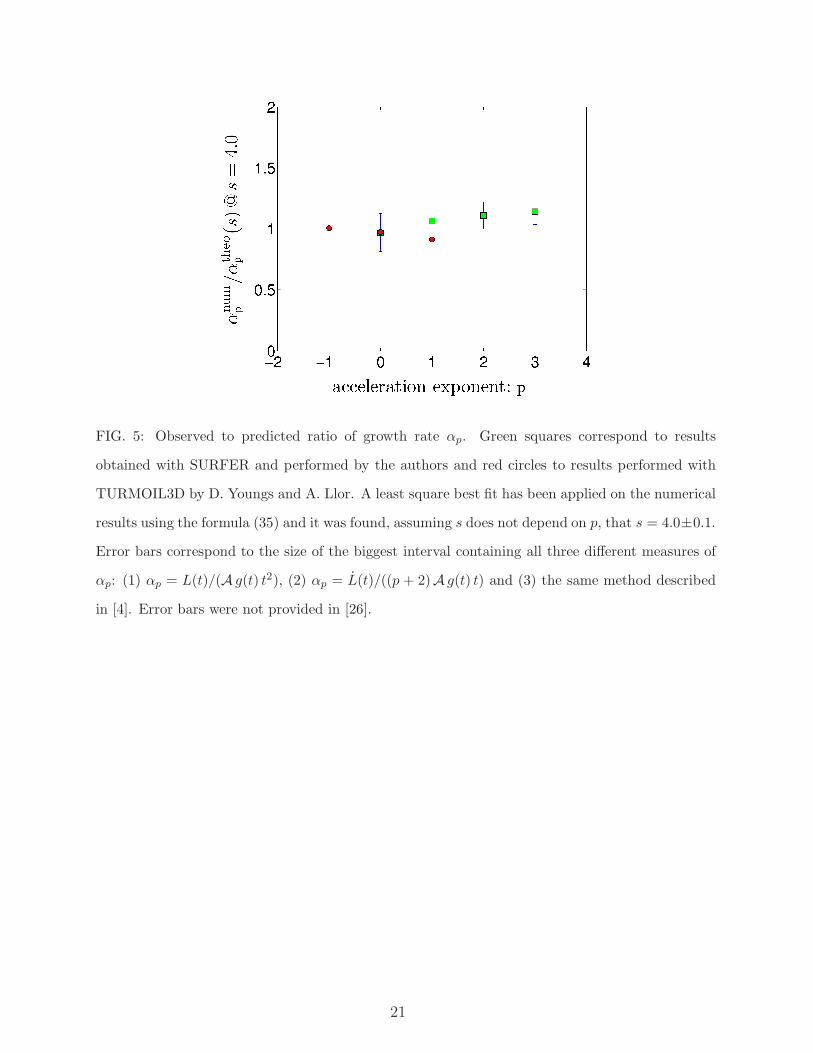
FIG. 5: Observed to predicted ratio of growth rate αp. Green squares correspond to results

obtained with SURFER and performed by the authors and red circles to results performed with

TURMOIL3D by D. Youngs and A. Llor. A least square best fit has been applied on the numerical

results using the formula (35) and it was found, assuming s does not depend on p, that s = 4.0±0.1.

Error bars correspond to the size of the biggest interval containing all three different measures of

αp: (1) αp = L(t)/(A g(t) t2), (2) αp = L(t)/((p + 2)A g(t) t) and (3) the same method described

in [4]. Error bars were not provided in [26].

21