arX

iv:1

003.

5949

v1 [

cond

-mat

.sta

t-m

ech]

30

Mar

201

0

Reliability of fluctuation-induced transport in a

Maxwell-demon-type engine

Raishma Krishnan,1, ∗ Sanjay Puri,1, † and Arun M. Jayannavar2

1School of Physical Sciences, Jawaharlal Nehru University, New Delhi – 110067, India.

2Institute of Physics, Sachivalaya Marg, Bhubaneswar – 751005, India.‡

Abstract

We study the transport properties of an overdamped Brownian particle which is simultaneously

in contact with two thermal baths. The first bath is modeled by an additive thermal noise at

temperature TA. The second bath is associated with a multiplicative thermal noise at temperature

TB . The analytical expressions for the particle velocity and diffusion constant are derived for this

system, and the reliability or coherence of transport is analyzed by means of their ratio in terms of

a dimensionless Peclet number. We find that the transport is not very coherent, though one can

get significantly higher currents.

∗Electronic address: raishma@gmail.com†Electronic address: purijnu@gmail.com‡Electronic address: jayan@iopb.res.in

1

I. INTRODUCTION

The second law of thermodynamics implies that it is not possible to get useful work from

a single heat bath at constant temperature. The perfect time-reversal symmetry (or detailed

balance) which exists under equilibrium conditions causes the flux in either direction to be

the same resulting in zero average flux. But advances in this area, especially in the context

of biological systems, show that it is possible to induce a directed motion provided there

exist some nonequilibrium fluctuations. These are usually provided by unbiased external

input agents. Devices which exploit these fluctuations to generate a unidirectional flow have

been termed as ratchets or Brownian motors. For a detailed discussion of these systems,

see [1].

The underlying thermal fluctuations are usually quantified in terms of temperature.

Though these fluctuations cannot be observed directly in macroscopic systems, the recent

advances in nanotechnology and molecular biology allow one to devise molecular systems

where they play a pivotal role. Thus, rather than trying to avoid these inherent fluctua-

tions, they have been utilized for constructive purposes: Brownian motors serve as the best

example of this.

Many different classes of model systems exist in the literature, and detailed studies have

been done with regard to transport and energetics in such systems. In our present work,

we consider a model of Brownian motor where the system has a space-dependent diffusion

coefficient D(x). The main emphasis in these systems is that the potential need not be

ratchet-like. Examples of such systems arise in semiconductor and superlattice structures,

molecular motor proteins moving along microtubules, etc. [2, 3].

A space-dependent diffusion coefficient D(x) could arise either due to a spatial variation

of temperature or friction coefficient, or both. For a system having a space-dependent

temperature [T (x)] the system dissipates energy during its evolution differently at different

places. This implies that the system is out of equilibrium. A similar effect arises in a

medium with a space-dependent friction coefficient [η(x)] in the presence of an external

noise [4–8]. To be more precise, frictional inhomogeneity does not generate any current by

itself - nonequilibrium fluctuations are crucial for transport in these systems.

It has been shown by Buttiker [8] that, in the presence of D(x), the Boltzmann factor

2

exp[−V (x)/kBT ] has to be generalized as exp[−ψ(x)] where

ψ(x) = −∫ x

dqv(q)

D(q). (1)

Here, v(x) = −µdV/dx is the drift velocity and µ is the mobility. For a homogeneous

system, D(x) is given by Einstein’s relation D = µkBT . The stability and dynamics of

nonequilibrium system is greatly influenced by the above generalized potential. Here, one

has to invoke the notion of global stability of states, as opposed to local stability which is

valid for equilibrium states [7].

In the present work, we consider a Brownian particle in contact with two thermal baths,

A and B. The underlying potential V (x) and the friction coefficient η(x) are periodic in

space, and separated by a phase difference other than 0 and π. We study the quality of

transport in such systems. Here, the unidirectional current arises due to a combination of

both η(x) and the fluctuations present in the second thermal bath.

Millonas [5] and Jayannavar [6] have analyzed the basic framework for particle transport

in such systems. Subsequently, Chaudhuri et al. [9] have also studied this model with

modifications in the bath parameters. However, there has been no systematic analysis of the

dependence of the current on system parameters. Further, there is no clear understanding

of the coherence of transport in these systems. In this paper, we undertake a detailed study

of both these properties.

The transport of a Brownian particle is always accompanied by a diffusive spread, and the

quality of transport is affected by this diffusive spread. This property has been quantified

via the ratio of current to the diffusion constant and is termed as the Peclet number, Pe.

The Brownian particle takes a time τ = L/v to traverse a distance L with a velocity v and

the diffusive spread of the particle in the same time is given by 〈(∆q)2〉 = 2Dτ . The criterion

to have a reliable transport is that 〈(∆q)2〉 = 2Dτ < L2. This implies that Pe= Lv/D > 2

for coherent transport. The Peclet numbers for some of the models like flashing and rocking

ratchets show low coherence of transport with Pe ∼ 0.2 and Pe ∼ 0.6 [10], respectively.

Experimental studies on molecular motors showed more reliable transport with Pe ranging

from 2 - 6 [11]. Our earlier work on inhomogeneous ratchets in the presence of a single heat

bath but, subjected to an external parametric white noise fluctuation, showed a coherent

transport with Pe of the order of 3 [12]. From this and other works [13], one concludes

that system inhomogeneities may enhance the effectiveness of transport, though sensitively

3

dependent on physical parameters.

The present paper is organised as follows. Section II gives the basic description of the

systems, and also the analytical expressions for current and diffusion needed to evaluate the

Peclet number. In Section III, we present detailed results for the dependence of current and

quality of transport on system parameters. In Section IV, we conclude this paper with a

brief summary.

II. MODEL

We begin with the equation of motion for a Brownian particle of massm and position x(t)

coupled simultaneously with (a) an additive thermal noise bath at temperature TA, and (b)

a multiplicative noise bath having a spatially-varying friction coefficient η(x) at temperature

TB. The particle moves in an underlying periodic potential V (x). The equation of motion

of the Brownian particle is given by [5, 6]

mx = −Γ(x)x− V ′(x) +√

η(x)ξB(t) + ξA(t). (2)

The Gaussian white noises ξA(t) and ξB(t) are independent, and obey the statistics:

〈ξA(t)〉 = 0, 〈ξA(t)ξA(t′)〉 = 2ΓAkBTAδ(t− t′), (3)

〈ξB(t)〉 = 0, 〈ξB(t)ξB(t′)〉 = 2ΓBkBTBδ(t− t′). (4)

The two noises together satisfy the fluctuation-dissipation theorem and Γ(x) = ΓA+ΓBη(x).

Here 〈...〉 denotes the ensemble average. In the present work, we have chosen V (x) =

V0(1−cosx) and η(x) = η0[1−λ cos(x−φ)]. Here 0 < λ < 1, and we set λ = 0.9 throughout

for optimum values. The phase lag φ between V (x) and η(x) brings in asymmetry in the

dynamics of the system. This inturn leads to an unidirectional current even in the presence

of spatially periodic (nonratchet-like) potential.

When the friction term dominates inertia or on time-scales larger than the inverse fric-

tion coefficient, one can consider the overdamped limit of the Langevin equation. This

corresponds to the adiabatic elimination of the fast variable (velocity) from the equation of

motion by putting p = x = 0. This approach is only applicable for a homogeneous system.

For an inhomogeneous system, Sancho et al. [14] have given the proper prescription for the

elimination of fast variables. The resultant overdamped Langevin equation for Eq. (2) is

4

given by [4]

x = −V′(x)

Γ(x)− (

√η(x))′√η(x)Γ2(x)

+ξA(t)

Γ(x)+

√η(x)

Γ(x)ξB(t). (5)

The prime on a function denotes differentiation with respect to x. Using the van Kampen

Lemma [15] and Novikov’s theorem [16], we obtain the corresponding Fokker-Planck equation

for the probability density P (x, t) of a particle to be at point x at time t as follows:

∂P (x, t)

∂t=

∂

∂x

{

V ′(x)

Γ(x)+TBΓB

Γ2(x)(√η(x))′√η(x)

}

P +TAΓA

Γ(x)

∂

∂x

[

P

Γ(x)

]

+ TBΓB

√η(x)

Γ(x)

∂

∂x

[√η(x)

Γ(x)P

]

. (6)

When the potential V (x) is positive and unbounded, the system evolves to a steady-state

distribution Ps(x) characterised by zero current. Setting J(x, t) = 0 in Eq. (6), we obtain

Ps(x) = N exp[−ψ(x)], (7)

where

ψ(x) =

∫ x

dq[ V ′(q)Γ(q)

TAΓA + TBΓBη(q)+

(TB − TA)

Γ(q)

ΓAΓBη′(q)TAΓA + TBΓBη(q)

]

. (8)

Here, ψ(x) is the dimensionless effective potential, and N is the normalization constant.

For periodic functions V (x) and η(x) with periodicity 2π, a finite probability current is

obtained. Following Risken [17], one readily gets the expression for the total probability

current J as

J =[1− exp (−2πδ)]

∫ 2π

0dy exp [−ψ(y)]

∫ y+2π

ydx exp [ψ(x)]/A(x)

. (9)

Here, δ determines the direction of current in the system and is given by

δ = ψ(x)− ψ(x+ 2π), (10)

and A(x) in Eq.( 9) is given by

A(x) =ΓATA + ΓBTBη(x)

Γ2(x). (11)

From Eqs. (8) - (10), we can see that the system is in equilibrium when TA = TB, leading

to zero net current. But when TA 6= TB, the system is rendered nonequilibrium and one can

extract energy at the expense of increased entropy. It can also be seen that no current is

possible when either ΓA or ΓB is absent. Again, if η(x) is independent of x, there will be no

net current flow in the system. When TA − TB changes sign, the current also changes sign

but not the magnitude.

5

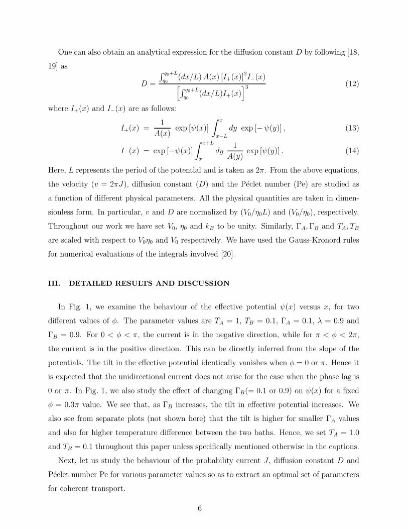
One can also obtain an analytical expression for the diffusion constant D by following [18,

19] as

D =

∫ q0+L

q0(dx/L)A(x) [I+(x)]

2I−(x)[

∫ q0+L

q0(dx/L)I+(x)

]3(12)

where I+(x) and I−(x) are as follows:

I+(x) =1

A(x)exp [ψ(x)]

∫ x

x−L

dy exp [−ψ(y)] , (13)

I−(x) = exp [−ψ(x)]∫ x+L

x

dy1

A(y)exp [ψ(y)] . (14)

Here, L represents the period of the potential and is taken as 2π. From the above equations,

the velocity (v = 2πJ), diffusion constant (D) and the Peclet number (Pe) are studied as

a function of different physical parameters. All the physical quantities are taken in dimen-

sionless form. In particular, v and D are normalized by (V0/η0L) and (V0/η0), respectively.

Throughout our work we have set V0, η0 and kB to be unity. Similarly, ΓA,ΓB and TA, TB

are scaled with respect to V0η0 and V0 respectively. We have used the Gauss-Kronord rules

for numerical evaluations of the integrals involved [20].

III. DETAILED RESULTS AND DISCUSSION

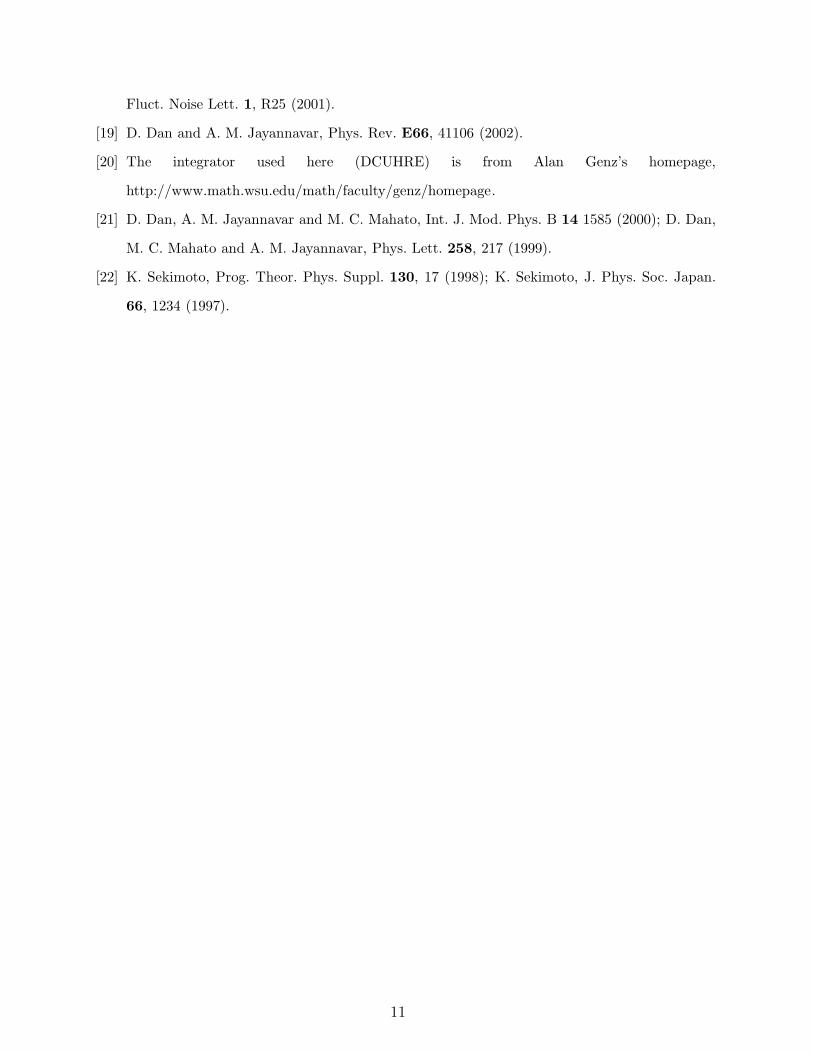
In Fig. 1, we examine the behaviour of the effective potential ψ(x) versus x, for two

different values of φ. The parameter values are TA = 1, TB = 0.1, ΓA = 0.1, λ = 0.9 and

ΓB = 0.9. For 0 < φ < π, the current is in the negative direction, while for π < φ < 2π,

the current is in the positive direction. This can be directly inferred from the slope of the

potentials. The tilt in the effective potential identically vanishes when φ = 0 or π. Hence it

is expected that the unidirectional current does not arise for the case when the phase lag is

0 or π. In Fig. 1, we also study the effect of changing ΓB(= 0.1 or 0.9) on ψ(x) for a fixed

φ = 0.3π value. We see that, as ΓB increases, the tilt in effective potential increases. We

also see from separate plots (not shown here) that the tilt is higher for smaller ΓA values

and also for higher temperature difference between the two baths. Hence, we set TA = 1.0

and TB = 0.1 throughout this paper unless specifically mentioned otherwise in the captions.

Next, let us study the behaviour of the probability current J , diffusion constant D and

Peclet number Pe for various parameter values so as to extract an optimal set of parameters

for coherent transport.

6

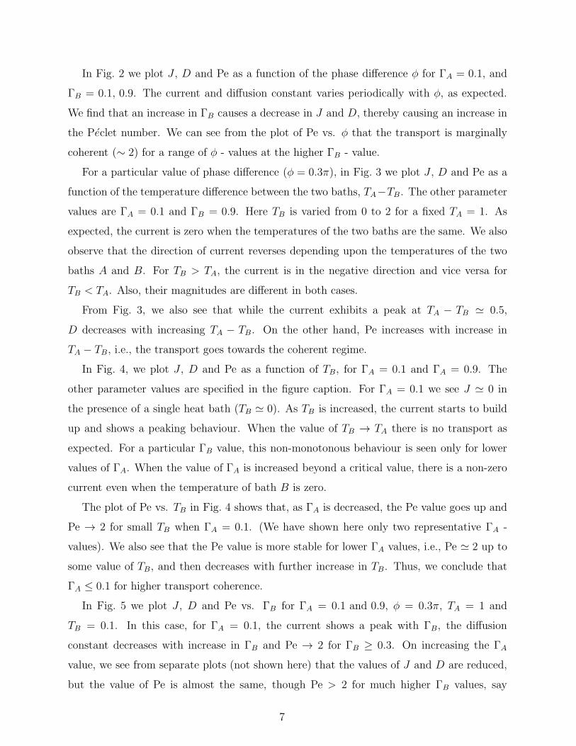
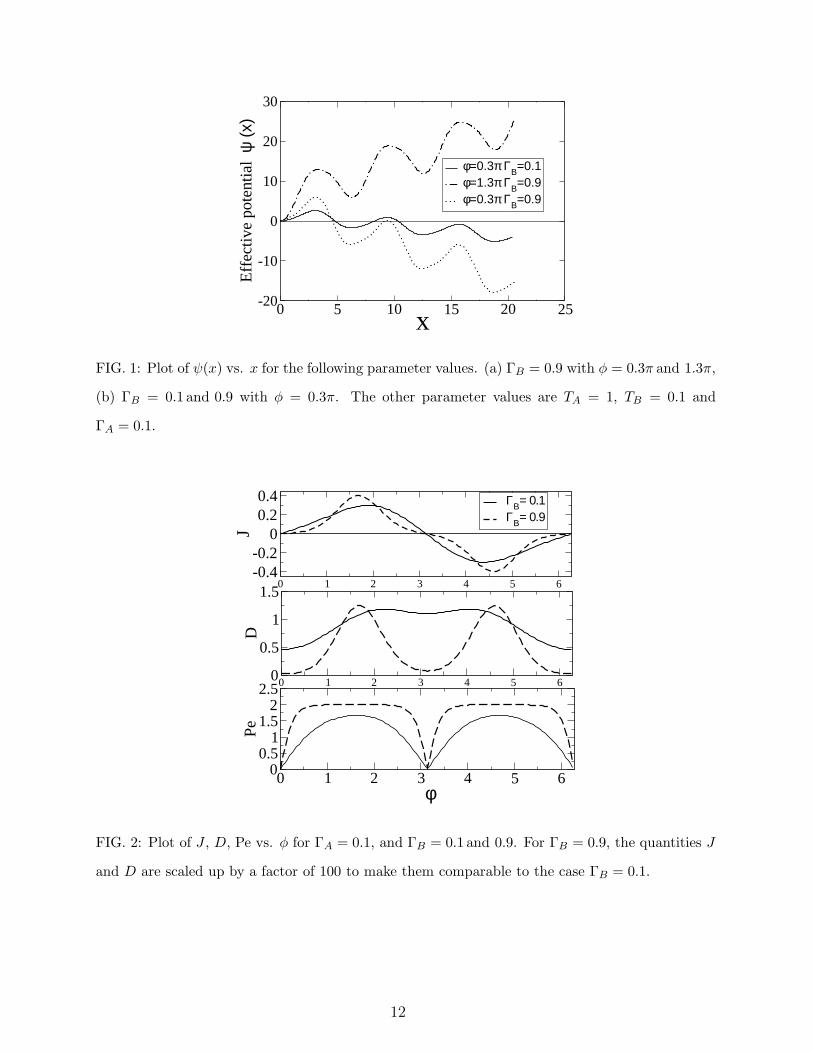
In Fig. 2 we plot J , D and Pe as a function of the phase difference φ for ΓA = 0.1, and

ΓB = 0.1, 0.9. The current and diffusion constant varies periodically with φ, as expected.

We find that an increase in ΓB causes a decrease in J and D, thereby causing an increase in

the Peclet number. We can see from the plot of Pe vs. φ that the transport is marginally

coherent (∼ 2) for a range of φ - values at the higher ΓB - value.

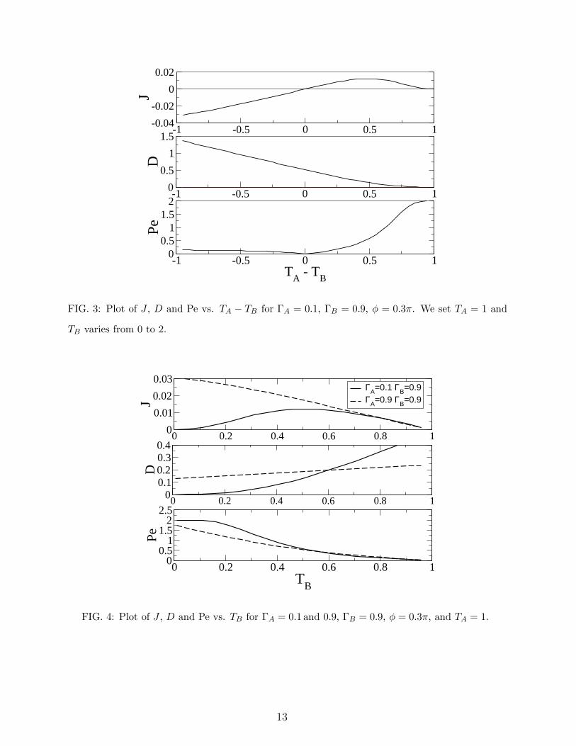
For a particular value of phase difference (φ = 0.3π), in Fig. 3 we plot J , D and Pe as a

function of the temperature difference between the two baths, TA−TB . The other parameter

values are ΓA = 0.1 and ΓB = 0.9. Here TB is varied from 0 to 2 for a fixed TA = 1. As

expected, the current is zero when the temperatures of the two baths are the same. We also

observe that the direction of current reverses depending upon the temperatures of the two

baths A and B. For TB > TA, the current is in the negative direction and vice versa for

TB < TA. Also, their magnitudes are different in both cases.

From Fig. 3, we also see that while the current exhibits a peak at TA − TB ≃ 0.5,

D decreases with increasing TA − TB. On the other hand, Pe increases with increase in

TA − TB, i.e., the transport goes towards the coherent regime.

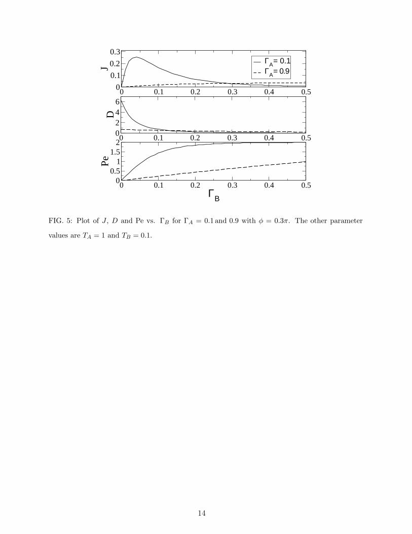
In Fig. 4, we plot J , D and Pe as a function of TB, for ΓA = 0.1 and ΓA = 0.9. The

other parameter values are specified in the figure caption. For ΓA = 0.1 we see J ≃ 0 in

the presence of a single heat bath (TB ≃ 0). As TB is increased, the current starts to build

up and shows a peaking behaviour. When the value of TB → TA there is no transport as

expected. For a particular ΓB value, this non-monotonous behaviour is seen only for lower

values of ΓA. When the value of ΓA is increased beyond a critical value, there is a non-zero

current even when the temperature of bath B is zero.

The plot of Pe vs. TB in Fig. 4 shows that, as ΓA is decreased, the Pe value goes up and

Pe → 2 for small TB when ΓA = 0.1. (We have shown here only two representative ΓA -

values). We also see that the Pe value is more stable for lower ΓA values, i.e., Pe ≃ 2 up to

some value of TB, and then decreases with further increase in TB. Thus, we conclude that

ΓA ≤ 0.1 for higher transport coherence.

In Fig. 5 we plot J , D and Pe vs. ΓB for ΓA = 0.1 and 0.9, φ = 0.3π, TA = 1 and

TB = 0.1. In this case, for ΓA = 0.1, the current shows a peak with ΓB, the diffusion

constant decreases with increase in ΓB and Pe → 2 for ΓB ≥ 0.3. On increasing the ΓA

value, we see from separate plots (not shown here) that the values of J and D are reduced,

but the value of Pe is almost the same, though Pe > 2 for much higher ΓB values, say

7

ΓB = 5. Thus, Fig. 5 also leads to the conclusion that a lower ΓA - value along with a higher

ΓB - value aids transport coherence.

IV. SUMMARY AND DISCUSSION

Let us conclude this paper with a brief summary and discussion. We have studied the

transport coherence of an overdamped Brownian particle in the presence of two thermal

baths, namely A and B with different noise statistics. One of the baths, B, is characterized

by the presence of a state-dependent friction coefficient. The system considered here is

analogous to a simple model of a Maxwell-demon-type of engine, which extracts work out

of the nonequilibrium state from thermal fluctuations by rectifying the internal fluctuations

in the system [5, 6]. The space-dependent friction coefficient in bath B is necessary for

generating unidirectional current in the absence of a bias. The direction of current (but not

its magnitude) changes sign when (TA − TB) changes sign. The current identically vanishes

when the temperatures of both the baths are the same. Also, in the extreme high friction

limit, the current vanishes as the particle cannot execute Brownian motion.

We have systematically analyzed the behaviour of current, diffusion and transport coher-

ence as a function of system parameters. The problem of coherence of transport has not

been addressed in the context of these systems. Our work demonstrates that a combination

of lower ΓA - value and a higher ΓB - value would lead to an optimum transport coherence.

Our study of the Peclet number shows that, for most of the parameter space, Pe ≤ 2. Thus,

we conclude from the present study that the transport is not coherent though it is possible

to get high current.

Our study can be extended in several directions. For example, it would be interesting

to study the efficiency of energy transduction in this Maxwell-demon-type heat engine by

using the methods of stochastic energetics developed by Sekimoto [22]. The fact that the

steady-state probability distribution Ps(x), Eq. (7) is a nonlocal function of V (x) and η(x)

itself can lead to much interesting physics and would form the basis of our future work.

8

Acknowledgements

R.K. gratefully acknowledges DST for financial support through a DST Fast-track project

[SR/FTP/PS-12/2009]. A.M.J. thanks DST for financial support. We also thank Mangal

C. Mahato and Sourabh Lahiri for useful discussions and help.

9

[1] P. Hanggi and F. Marchesoni, Rev. Mod. Phys. 81, 387 (2009); P. Reimann, Phys. Rep. 361,

57 (2002); H. Linke, Appl. Phys. A 75, 167-352 (2002).

[2] R. H. Luchsinger, Phys. Rev. E62, 272 (2000).

[3] M. C. Mahato and A. M. Jayannavar, Resonance 8, No:7, 33 (2003), M. C. Mahato and A.

M. Jayannavar, Resonance 8, No:9, 4 (2003).

[4] M. C. Mahato, T. P. Pareek and A. M. Jayannavar, Int. J. Mod. Phys. B 10, 3857 (1996);

A. M. Jayannavar and M. C. Mahato, Pramana-J. Phys. 45, 369 (1995); A. M. Jayannavar,

cond-mat 0107080.

[5] M. M. Millonas, Phys. Rev. Lett. 74, 10 (1995), Phys. Rev. Lett. 75, 3027 (1995) .

[6] A. M. Jayannavar, Phys. Rev. E53, 2957 (1996).

[7] R. Landauer, J. Stat. Phys. 53, 233 (1988).

[8] M. Buttiker, Z. Phys. B 68,161 (1987).

[9] J. R. Chaudhuri, S. Chattopadhyay and S. K. Banik, The Journal of Chem. Phys. 127, 224508

(2007).

[10] J. A. Freund and L. Schimansky-Geier, Phys. Rev. E60, 1304 (1999); T. Harms and R.

Lipowsky, Phys. Rev. Lett. 79, 2895 (1997).

[11] M. J. Schnitzer and S. M. Block, Nature (London) 388, 386 (1997); K. Visscher, M. J.

Schnitzer and S. M. Block, Nature 400, 184 (1999).

[12] R. Krishnan, D. Dan and A. M. Jayannavar, Mod. Phys. Lett. B 19 Nos 19 & 20, 971 (2005);

R. Krishnan, D. Dan and A. M. Jayannavar, Physica A 354, 171 (2005); R. Krishnan, D. Dan

and A. M. Jayannavar, Ind. J. Phys. 78, 747 (2004).

[13] B. Linder and L Schimansky-Geier, Phys. Rev. Lett. 89, 230602 (2002).

[14] J. M. Sancho, M. San Miguel and D. Duerr, J. Stat. Phys. 28, 291 (1982).

[15] N. G. van Kampen, Phys. Rep. C24, 172 (1976).

[16] E. A. Novikov, Zh. Eksp. Teor. Fiz. 47, 1919 (1964); Sov. Phys. JETP 20, 1290 (1965).

[17] H. Risken, The Fokker-Planck Equation (Springer Verlag, Berlin, 1984).

[18] P. Reimann, C. Van den Broeck, H. Linke, P. Hanggi, J. M. Rubi and A. Perez-Madrid, Phys.

Rev. E65, 31104 (2002); P. Reimann, C. Van den Broeck, H. Linke, P. Hanggi, J. M. Rubi

and A. Perez-Madrid, Phys. Rev. Lett. 87,10602 (2001); B. Linder and L. Schimansky-Geier,

10

Fluct. Noise Lett. 1, R25 (2001).

[19] D. Dan and A. M. Jayannavar, Phys. Rev. E66, 41106 (2002).

[20] The integrator used here (DCUHRE) is from Alan Genz’s homepage,

http://www.math.wsu.edu/math/faculty/genz/homepage.

[21] D. Dan, A. M. Jayannavar and M. C. Mahato, Int. J. Mod. Phys. B 14 1585 (2000); D. Dan,

M. C. Mahato and A. M. Jayannavar, Phys. Lett. 258, 217 (1999).

[22] K. Sekimoto, Prog. Theor. Phys. Suppl. 130, 17 (1998); K. Sekimoto, J. Phys. Soc. Japan.

66, 1234 (1997).

11

0 5 10 15 20 25x

-20

-10

0

10

20

30

Eff

ectiv

e po

tent

ial

ψ (x

)

φ=0.3π ΓB=0.1 φ=1.3π ΓB=0.9 φ=0.3π ΓB=0.9

FIG. 1: Plot of ψ(x) vs. x for the following parameter values. (a) ΓB = 0.9 with φ = 0.3π and 1.3π,

(b) ΓB = 0.1 and 0.9 with φ = 0.3π. The other parameter values are TA = 1, TB = 0.1 and

ΓA = 0.1.

0 1 2 3 4 5 6-0.4-0.2

00.20.4

J

ΓΒ= 0.1 ΓΒ= 0.9

0 1 2 3 4 5 60

0.5

1

1.5

D

0 1 2 3 4 5 6 φ

00.5

11.5

22.5

Pe

FIG. 2: Plot of J , D, Pe vs. φ for ΓA = 0.1, and ΓB = 0.1 and 0.9. For ΓB = 0.9, the quantities J

and D are scaled up by a factor of 100 to make them comparable to the case ΓB = 0.1.

12

-1 -0.5 0 0.5 1-0.04

-0.02

0

0.02

J

-1 -0.5 0 0.5 10

0.5

1

1.5

D

-1 -0.5 0 0.5 1T

A - T

B

00.5

11.5

2

Pe

FIG. 3: Plot of J , D and Pe vs. TA − TB for ΓA = 0.1, ΓB = 0.9, φ = 0.3π. We set TA = 1 and

TB varies from 0 to 2.

0 0.2 0.4 0.6 0.8 10

0.01

0.02

0.03

J

ΓA=0.1 ΓB=0.9ΓA=0.9 ΓB=0.9

0 0.2 0.4 0.6 0.8 10

0.10.20.30.4

D

0 0.2 0.4 0.6 0.8 1T

B

00.5

11.5

22.5

Pe

FIG. 4: Plot of J , D and Pe vs. TB for ΓA = 0.1 and 0.9, ΓB = 0.9, φ = 0.3π, and TA = 1.

13

0 0.1 0.2 0.3 0.4 0.50

0.1

0.2

0.3

J

ΓΑ= 0.1ΓΑ= 0.9

0 0.1 0.2 0.3 0.4 0.50246

D

0 0.1 0.2 0.3 0.4 0.5ΓB

00.5

11.5

2

Pe

FIG. 5: Plot of J , D and Pe vs. ΓB for ΓA = 0.1 and 0.9 with φ = 0.3π. The other parameter

values are TA = 1 and TB = 0.1.

14