Bridge System Reliability and Reliability-Based Redundancy ...
62
Bridge System Reliability and Reliability Based Redundancy Factors September 16, 2019 Sponsored by Federal Highway Administration Office of Infrastructure – Bridges and Structures FHWA-HIF-19-093
-
Upload
khangminh22 -
Category
Documents
-
view
2 -
download
0
Transcript of Bridge System Reliability and Reliability-Based Redundancy ...
Bridge System Reliability and ReliabilityBased Redundancy Factors
September 16, 2019
Sponsored by Federal Highway AdministrationOffice of Infrastructure – Bridges and Structures FHWA-HIF-19-093

ForewordThis report provides documentation of a research effort to study the system reliability of bridge structures, which was performed by Lehigh University in cooperation with Federal Highway Administration. This research provides deep insights into the relationship between component and system reliability in bridges, and gives practical recommendations for improving the redundancy factor that is used in LRFD design methodology.
If the recommendations from this effort are implemented, more uniform and consistent system reliability will be achievable for different bridge types, layouts, and properties of components.
Joseph L. Hartmann, PhD, P.E.Director, Office of Bridges and Structures
NoticeThis document is disseminated under the sponsorship of the U.S. Department of Transportation in the interest of information exchange. The U.S. Government assumes no liability for the use of the information contained in this document.
The U.S. Government does not endorse products or manufacturers. Trademarks or manufacturers’ names appear in this report only because they are considered essential to the objective of the document.
Quality Assurance StatementThe Federal Highway Administration (FHWA) provides high-quality information to serve Government, industry, and the public in a manner that promotes public understanding. Standards and policies are used to ensure and maximize the quality, objectivity, utility, and integrity of its information. FHWA periodically reviews quality issues and adjusts its programs and processes to ensure continuous quality improvement.

1. Report No.
FHWA-HIF-19-093
2. Government Accession No. 3. Recipient’s Catalog No.
4. Title and Subtitle
Bridge System Reliability and Reliability-Based Redundancy Factors
5. Report Date
September 2019
6. Performing Organization Code
7. Author(s) Dan M. Frangopol, Benjin Zhu, Samantha Sabatino, and Brian Kozy
8. Performing Organization Report No.
9. Performing Organization Name and Address
ATLSS Engineering Research CenterLehigh University117 ATLSS DriveBethlehem, PA 18015
10. Work Unit No.
11. Contract or Grant No.
DTFH61-11-H-00027
12. Sponsoring Agency Name and Address
Federal Highway AdministrationOffice of Infrastructure – Bridges and Structures1200 New Jersey Ave.SE Washington, DC 20590
13. Type of Report and Period Covered
Final Report September 2017 to August 2019
14. Sponsoring Agency Code
15. Supplementary Notes
Work funded by Cooperative Agreement “Advancing Steel and Concrete Bridge Technology to Improve Infrastructure Performance” between FHWA and Lehigh University.
16. Abstract
This report proposes a redundancy factor to provide improved bridge system reliability using conventional component-based limit-state design. The redundancy factor is based on a system reliability assessment, and it provides a missing link between bridge component reliability and bridge system reliability. It is intended to provide more uniform bridge system reliability across bridge system types. Focus is placed on critical (i.e., strength) limit states. The effects of the system model type, correlation among the component resistances, and coefficients of variation for the component load effects and resistances on the system reliability and the redundancy factor are shown for systems with up to 100 components.
17. Key Words
Bridges, reliability, redundancy, structural reliability, structural redundancy, system reliability, redundancy factor
18. Distribution Statement
No restrictions. This document is available through the National Technical Information Service, Springfield, VA 22161
9. Security Classif. (of this report)
Unclassified
20. Security Classif. (of this page)
Unclassified
21. No of Pages
51
22. Price
Free


i
Table of Contents1. INTRODUCTION ...................................................................................................................... 1
1.1 MODELS FOR CALCULATING SYSTEM RELIABILITY ............................................. 1
1.2 SYSTEM MODEL TYPES .................................................................................................. 3
1.3 REDUNDANCY FACTOR .................................................................................................. 4
1.4 OVERVIEW OF REPORT ................................................................................................... 5
2. RELIABILITY OF BRIDGE SYSTEMS WITH EQUALLY RELIABLE COMPONENTS ................................................................................................................. 6
2.1 CALCULATING SYSTEM RELIABILITY WITH EQUALLY RELIABLE COMPONENTS ............................................................................................................. 6
2.2 EXAMPLE: A THREE-COMPONENT SYSTEM .............................................................. 7
2.3 EFFECTS OF V(R), V(P), E(P), Ρ(RI,RJ) AND N ON SYSTEM RELIABILITY .............. 7
2.4 RELIABILITY OF SYSTEMS WITH MANY EQUALLY RELIABLE COMPONENTS ........................................................................................................... 11
2.5 APPLICATION OF SYSTEM RELIABILITY RESULTS ............................................... 12
3. RELIABILITY-BASED REDUNDANCY FACTORS ........................................................... 14
3.1 DEFINITION OF REDUNDANCY FACTOR .................................................................. 14
3.2 EXAMPLE: A THREE-COMPONENT SYSTEM ............................................................ 14
3.3 EFFECTS OF V(R), V(P), E(P) AND N ON REDUNDANCY FACTOR ........................ 15
3.4 REDUNDANCY FACTOR FOR SYSTEMS WITH MANY EQUALLY RELIABLE COMPONENTS ....................................................................................... 19
3.5 APPLICATION OF REDUNDANCY FACTOR RESULTS ............................................ 20
3.6 APPLICATION OF REDUNDANCY FACTOR IN COMPONENT DESIGN ................ 23
4. RELIABILITY-BASED REDUNDANCY FACTORS FOR DUCTILE AND BRITTLE SYSTEMS ....................................................................................................... 25
4.1 REDUNDANCY FACTOR FOR DUCTILE SYSTEMS ................................................. 25
4.2 REDUNDANCY FACTOR FOR BRITTLE SYSTEMS .................................................. 27

ii
4.3 REDUNDANCY FACTOR FOR MIXED DUCTILE-BRITTLE SYSTEMS ................. 31
4.4 SUMMARY OF REDUNDANCY FACTORS FOR DUCTILE AND BRITTLE SYSTEMS .................................................................................................................... 32
5. SUMMARY AND CONCLUSIONS ....................................................................................... 33
REFERENCES ............................................................................................................................. 35
APPENDIX I. RELIABILITY OF SYSTEMS WITH EQUALLY RELIABLE COMPONENTS ............................................................................................................... 36
APPENDIX II. RELIABILITY-BASED REDUNDANCY FACTORS ...................................... 40
iii
List of FiguresFigure 1. Illustration. Examples of system models. ........................................................................ 2
Figure 2. Illustration. System model types. .................................................................................... 3
Figure 3. Illustration. Simple truss example: (a) 5-member truss, (b) series system model. .......... 4
Figure 4. Illustration. Alternative 4-girder bridge system models: (a) series, (b) parallel, and (c) 2p×3s SP. ................................................................................................................ 4
Figure 5. Graph. Effects of (a) V(R); (b) V(P); and (c) E(P) on βsys for two-component systems for cases of no correlation and perfect correlation among resistances. ................. 8
Figure 6. Illustration. Four-component systems: (a) series system; (b) parallel system; and (c) series-parallel (SP) system. ........................................................................................... 8
Figure 7. Graph. Effects of V(R) on βsys for four-component systems for cases of: (a) no correlation; (b) partial correlation; and (c) perfect correlation among resistances. ............ 9
Figure 8. Graph. Effects of V(P) on βsys for four-component systems for cases of: (a) no correlation; (b) partial correlation; and (c) perfect correlation among resistances. .......... 10
Figure 9. Graph. Effects of number of components on βsys with variation of: (a) V(R); (b) V(P); and (c) E(P) for cases of no correlation and perfect correlation among resistances. ........................................................................................................................ 10
Figure 10. Graph. Effect of number of components on βsys when R and P have normal or lognormal distributions (Note: “N” denotes normal distribution; “LN” denotes lognormal distribution; “0” denotes ρ(Ri,Rj) = 0; and “0.5” denotes ρ(Ri,Rj) = 0.5). ................................................................................................................................... 12
Figure 11. Graph. Effects of: (a) V(R); (b) V(P); and (c) E(P) on ηR for twocomponent systems. ............................................................................................................................. 16
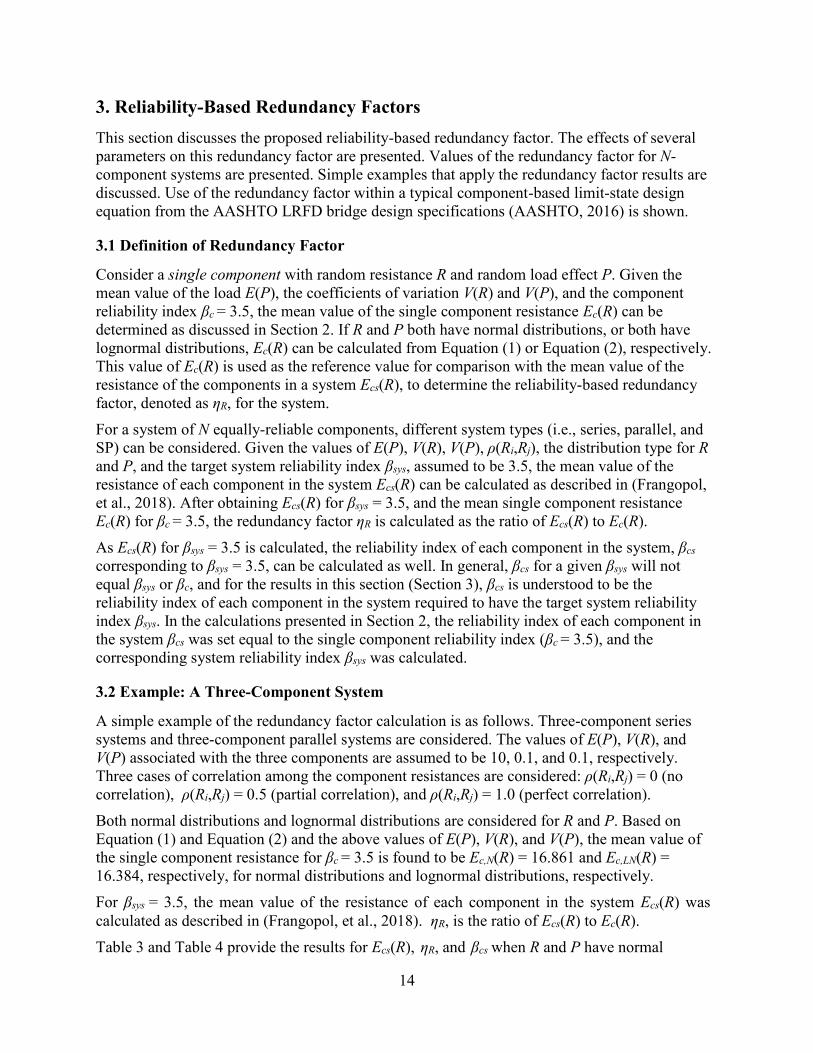
Figure 12. Graph. Effects of: (a) V(R); and (b) V(P) on Ec(R) and Ecs(R) for twocomponent systems. .......................................................................................................... 17
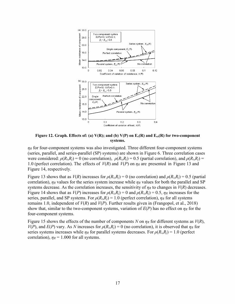
Figure 13. Graph. Effects of V(R) on ηR for fourcomponent systems for cases of: (a) no correlation; (b) partial correlation; and (c) perfect correlation among resistances. .......... 18
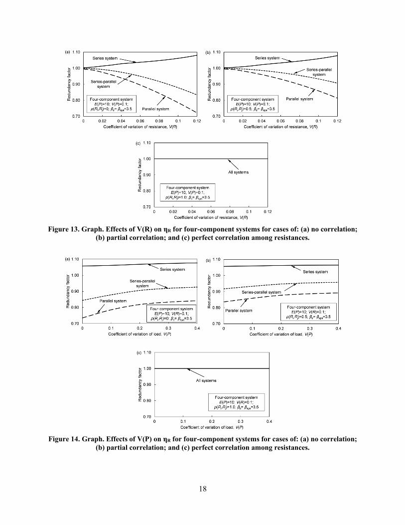
Figure 14. Graph. Effects of V(P) on ηR for fourcomponent systems for cases of: (a) no correlation; (b) partial correlation; and (c) perfect correlation among resistances. .......... 18

iv
Figure 15. Graph. Effects of number of components on ηR with variation of: (a) V(R); (b) V(P); and (c) E(P) for cases of no correlation and perfect correlation among resistances. ........................................................................................................................ 19
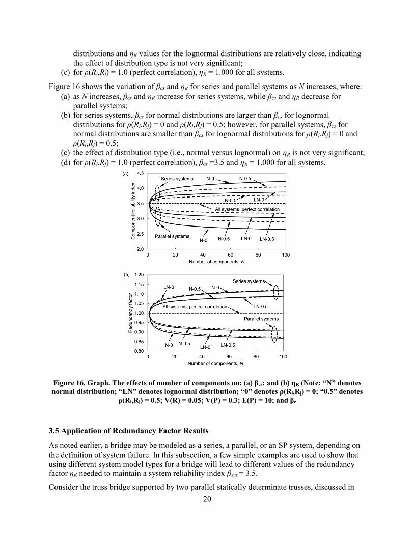
Figure 16. Graph. The effects of number of components on: (a) βcs; and (b) ηR (Note: “N” denotes normal distribution; “LN” denotes lognormal distribution; “0” denotes ρ(Ri,Rj) = 0; “0.5” denotes ρ(Ri,Rj) = 0.5; V(R) = 0.05; V(P) = 0.3; E(P) = 10; and βc ....................................................................................................................................... 20
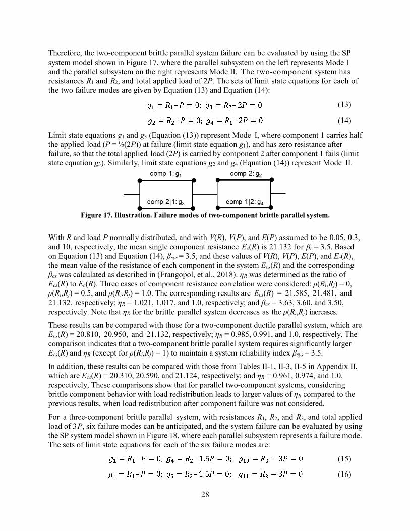
Figure 17. Illustration. Failure modes of two-component brittle parallel system. ........................ 28
Figure 18. Illustration. Failure modes of three-component brittle parallel system. ...................... 29
Figure 19. Illustration. Failure modes of four-component brittle series-parallel system.............. 30
Figure 20. Graph. Effects of number of brittle components on redundancy factor for four-component mixed parallel systems. .................................................................................. 32
v
List of Tables
Table 1. βsys for three-component systems when R and P have normal distributions. ................... 7
Table 2. βsys for three-component systems when R and P have lognormal distributions. .............. 7
Table 3. Ecs(R), ηR, and βcs for three-component systems when R and P have normal distributions.................................................................................................................... 15
Table 4. Ecs(R), ηR, and βcs for three-component systems when R and P have lognormal distributions.................................................................................................................... 15
Table 5. ηR and βcs for steel 4-girder bridge systems for Case A (V(R) = 0.05, V(P) = 0.3). ................................................................................................................................ 23
Table 6. ηR and βcs for steel 4-girder bridge systems for Case B (V(R) = 0.1, V(P) = 0.4). ........ 23
Table 7. Ecs(R), ηR and βcs for three-component ductile parallel systems when R and P have normal or lognormal distributions. ........................................................................ 26
Table 8. Ecs(R), ηR and βcs for four-component ductile systems when R and P have normal distributions. ...................................................................................................... 27
Table I- 1. βsys for different systems with 1 ≤ N ≤ 20 for different correlation cases when R and P have normal distributions. ................................................................................ 36
Table I- 2. βsys for different systems with 25 ≤ N ≤ 100 for different correlation cases when R and P have normal distributions. ...................................................................... 37
Table I- 3. βsys for different systems with 1 ≤ N ≤ 20 for different correlation cases when R and P have lognormal distributions. ........................................................................... 38
Table I- 4. βsys for different systems with 25 ≤ N ≤ 100 for different correlation cases when R and P have lognormal distributions. ................................................................. 39
Table II-1. Ecs(R) and ηR for different systems with 1 ≤ N ≤ 20 for ρ(Ri,Rj) = 0.0 when R and P have normal distributions. .................................................................................... 40
Table II- 2. Ecs(R) and ηR for different systems with 25 ≤ N ≤ 100 for ρ(Ri,Rj) = 0 when R and P have normal distributions. .................................................................................... 41

vi
Table II- 3. Ecs(R) and ηR for different systems with 1 ≤ N ≤ 20 for ρ(Ri,Rj) = 0.5 when R and P have normal distributions. .................................................................................... 42
Table II- 4. Ecs(R) and ηR for different systems with 25 ≤ N ≤ 100 for ρ(Ri,Rj) = 0.5 when R and P have normal distributions. ................................................................................ 43
Table II- 5. Ecs(R) and ηR for different systems with 1 ≤ N ≤ 20 for ρ(Ri,Rj) = 1.0 when R and P have normal distributions. .................................................................................... 44
Table II- 6. Ecs(R) and ηR for different systems with 25 ≤ N ≤ 100 for ρ(Ri,Rj) = 1.0 when R and P have normal distributions. ................................................................................ 45
Table II- 7. Ecs(R) and ηR for different systems with 1 ≤ N ≤ 25 for ρ(Ri,Rj) = 0 when R and P have lognormal distributions................................................................................ 46
Table II- 8. Ecs(R) and ηR for different systems with 50 ≤ N ≤ 100 for ρ(Ri,Rj) = 0.0 when R and P have lognormal distributions. ........................................................................... 47
Table II- 9. Ecs(R) and ηR for different systems with 1 ≤ N ≤ 25 for ρ(Ri,Rj) = 0.5 when R and P have lognormal distributions................................................................................ 48
Table II- 10. Ecs(R) and ηR for different systems with 50 ≤ N ≤ 100 for ρ(Ri,Rj) = 0.5 when R and P have lognormal distributions. ................................................................. 49
Table II- 11. Ecs(R) and ηR for different systems with 1 ≤ N ≤ 25 for ρ(Ri,Rj) = 1.0 when R and P have lognormal distributions. ........................................................................... 50
Table II- 12. Ecs(R) and ηR for different systems with 50 ≤ N ≤ 100 for ρ(Ri,Rj) = 1.0 when R and P have lognormal distributions. ................................................................. 51

vii
List of Abbreviations
AASHTO American Association of State Highway and Transportation Officials
LRFD Load and Resistance Factor Design
MCS Monte Carlo Simulation
SP Series-Parallel

1
1. IntroductionThe load and resistance factor design (LRFD) approach in modern structural design specifications is a reliability-based approach in which the uncertainties associated with the loads acting on a structure and the resistance of the structural components and connections are incorporated quantitatively into the design provisions. In the AASHTO LRFD bridge design specifications (AASHTO, 2016), the load and resistance factors for strength limit states are developed from the theory of reliability, based on current knowledge of the variability of load effects and of the resistance properties of bridge structural components and connections. In the process of calibrating the load and resistance factors, a target reliability index is used to provide an acceptable level of safety, and the load and resistance factors are determined to achieve a uniform level of reliability for the components and connections of a bridge for applicable limit states. The target reliability index is enforced for the individual components and connections rather than the bridge system. For the AASHTO LRFD bridge design specifications (AASHTO, 2016), the target reliability index for bridge structural components is 3.5.Structural system reliability is determined by considering failure of the system rather than failure of a single component. The system reliability is affected by component reliability, and by several other parameters, such as correlation among the component resistances and the system type. For some systems, the system reliability may be greater than the component reliability. For other systems, the system reliability may be less than the component reliability. AASHTO LRFD bridge design specifications (AASHTO, 2016), addresses these potential differences in system reliability with a simple, optional redundancy factor ranging from 0.95 to 1.05 that may be applied to the load effects. Recent work funded by FHWA and reported in (Frangopol, et al., 2018)addresses the system reliability and redundancy of bridge systems. This report summarizes results from this work.
1.1 Models for Calculating System Reliability
In this work, the models used to quantify system reliability of bridges are based on a simple representation of the actual bridge structural system. A system model represents a bridge as an idealized assembly of components with potential for failure. The components of the system model reflect the physical structural components and connections of a bridge (e.g. girders, truss members, etc.) and their potential limit states. Failure of a model component represents a primary structural component or connection of the bridge reaching a critical limit state. This definition is consistent with a typical component reliability assessment, where the load effect and resistance for a specific limit state are compared. The components of a system model are defined and arranged to reflect physical relationships among the structural components and connections of the bridge. For example, in some bridge systems or subsystems, certain structural components work in parallel with each other, and while in other bridge systems or subsystems, certain structural components work in series. Note that one structural component, such as a girder, may be represented by several model components in the system model, if several structural details and limit states need to be considered. Analysis of a system model does not require a structural analysis of the bridge, but the system model depends on assumptions about load distribution in the system (i.e., assumptions regarding the load effects for the model components). The loads acting on the bridge are assumed to be distributed to the model components. Uncertainty in the overall loading on the bridge is
2
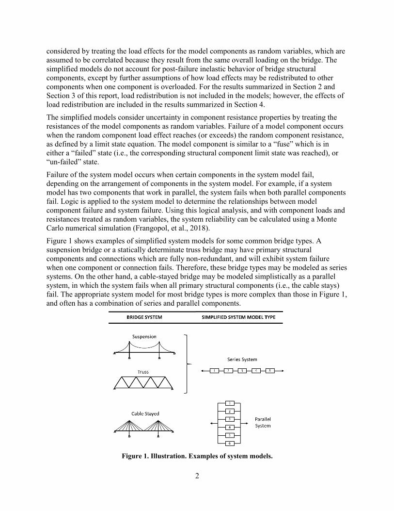
considered by treating the load effects for the model components as random variables, which are assumed to be correlated because they result from the same overall loading on the bridge. The simplified models do not account for post-failure inelastic behavior of bridge structural components, except by further assumptions of how load effects may be redistributed to other components when one component is overloaded. For the results summarized in Section 2 and Section 3 of this report, load redistribution is not included in the models; however, the effects of load redistribution are included in the results summarized in Section 4. The simplified models consider uncertainty in component resistance properties by treating the resistances of the model components as random variables. Failure of a model component occurs when the random component load effect reaches (or exceeds) the random component resistance, as defined by a limit state equation. The model component is similar to a “fuse” which is in either a “failed” state (i.e., the corresponding structural component limit state was reached), or “un-failed” state.Failure of the system model occurs when certain components in the system model fail, depending on the arrangement of components in the system model. For example, if a system model has two components that work in parallel, the system fails when both parallel components fail. Logic is applied to the system model to determine the relationships between model component failure and system failure. Using this logical analysis, and with component loads and resistances treated as random variables, the system reliability can be calculated using a Monte Carlo numerical simulation (Frangopol, et al., 2018).Figure 1 shows examples of simplified system models for some common bridge types. A suspension bridge or a statically determinate truss bridge may have primary structural components and connections which are fully non-redundant, and will exhibit system failure when one component or connection fails. Therefore, these bridge types may be modeled as series systems. On the other hand, a cable-stayed bridge may be modeled simplistically as a parallel system, in which the system fails when all primary structural components (i.e., the cable stays) fail. The appropriate system model for most bridge types is more complex than those in Figure 1, and often has a combination of series and parallel components.
Figure 1. Illustration. Examples of system models.
3
1.2 System Model Types
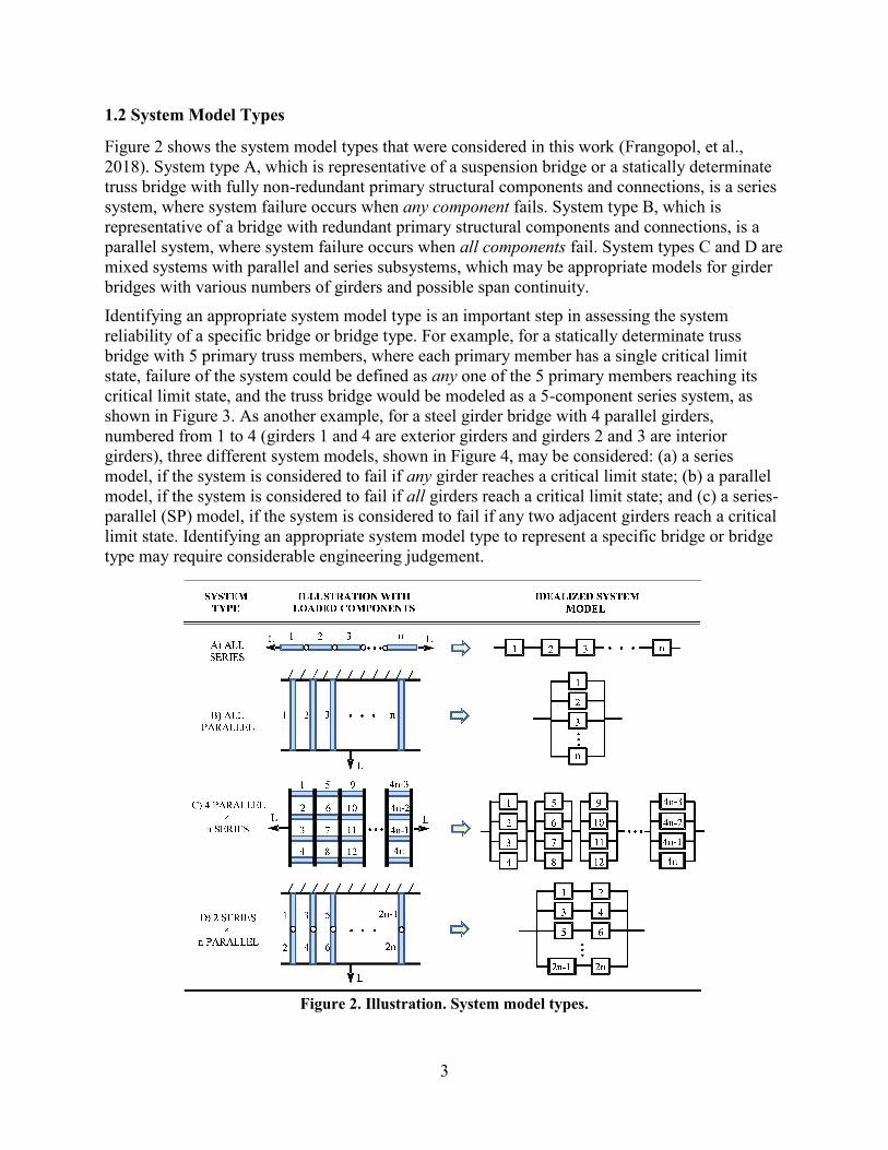
Figure 2 shows the system model types that were considered in this work (Frangopol, et al., 2018). System type A, which is representative of a suspension bridge or a statically determinate truss bridge with fully non-redundant primary structural components and connections, is a series system, where system failure occurs when any component fails. System type B, which is representative of a bridge with redundant primary structural components and connections, is a parallel system, where system failure occurs when all components fail. System types C and D are mixed systems with parallel and series subsystems, which may be appropriate models for girder bridges with various numbers of girders and possible span continuity.Identifying an appropriate system model type is an important step in assessing the system reliability of a specific bridge or bridge type. For example, for a statically determinate truss bridge with 5 primary truss members, where each primary member has a single critical limit state, failure of the system could be defined as any one of the 5 primary members reaching its critical limit state, and the truss bridge would be modeled as a 5-component series system, as shown in Figure 3. As another example, for a steel girder bridge with 4 parallel girders, numbered from 1 to 4 (girders 1 and 4 are exterior girders and girders 2 and 3 are interior girders), three different system models, shown in Figure 4, may be considered: (a) a series model, if the system is considered to fail if any girder reaches a critical limit state; (b) a parallel model, if the system is considered to fail if all girders reach a critical limit state; and (c) a series-parallel (SP) model, if the system is considered to fail if any two adjacent girders reach a critical limit state. Identifying an appropriate system model type to represent a specific bridge or bridge type may require considerable engineering judgement.
Figure 2. Illustration. System model types.

4
The research summarized in this report uses general system model types that are representative of common bridge types, and uses these general system model types to provide understanding of the key parameters that affect bridge system reliability. Although the simplified system models do not include a rigorous treatment of structural system response as structural components and connections reach critical limit states, these models are powerful tools for quantifying bridge system reliability and the relationships between component reliability and system reliability, and enable the influence of key parameters to be studied efficiently, as shown in this report.
Figure 4. Illustration. Alternative 4-girder bridge system models: (a) series, (b) parallel, and (c) 2p×3s SP.
1.3 Redundancy Factor
The AASHTO LRFD bridge design specifications (AASHTO, 2016) include a factor relating to redundancy ηR to be applied to load effects. Its value is determined as follows:
(a) ηR ≥ 1.05 for nonredundant members;(b) ηR = 1.00 for conventional level of redundancy;(c) ηR ≥ 0.95 for exceptional levels of redundancy.
These classes of redundancy for establishing the redundancy factor ηR in the AASHTO LRFD bridge design specifications (AASHTO, 2016) are general and based on engineering judgement. As shown by the results presented in this report, the value of a reliability-based redundancy factor is influenced by several parameters, such as the system model type, number of components in the system, and the correlation among the component resistances. Therefore, as mentioned in Section 1.3.2.1 of the AASHTO LRFD bridge design specifications (AASHTO, 2016), “improved quantification of ductility, redundancy, and operational classification may be attained with time, and possibly leading to a rearranging of Eq. 1.3.2.1-1, in which these effects may appear on either side of the equation or on both sides”.In Section 3 of this report, a reliability-based redundancy factor ηR is proposed to account for redundancy on either the load or the resistance side of the limit state equation.
Figure 3. Illustration. Simple truss example: (a) 5-member truss, (b) series system model.

5
1.4 Overview of Report
Section 2 of the report presents results for reliability of systems with components that have a target component reliability index of 3.5. Results for various system model types with varying numbers of components are presented. The effects of several parameters on the system reliability are shown. Simple examples that apply the system reliability results are presented.Section 3 of the report presents results for the reliability-based redundancy factor ηR. Results for various system model types with varying numbers of components are presented. The effects of several parameters are shown and simple examples that apply the reliability-based redundancy factor are given. Application of the reliability-based redundancy factor within a typical component-based limit-state design equation from the AASHTO LRFD bridge design specifications (AASHTO, 2016) is shown.Section 4 of the report presents results to illustrate the effects of the load redistribution that may occur when a structural component exhibits ductile or brittle behavior as a critical limit state is reached. The effects of load redistribution for ductile, brittle, and mixed systems on the reliability-based redundancy factor are shown.
6
2. Reliability of Bridge Systems with Equally Reliable ComponentsThe system reliability of bridge systems with N equally reliable components is presented in this section. The effects of several parameters on the system reliability when the system components have the target reliability index of 3.5 are presented. Results for the system reliability index of various N-component systems are presented. Simple examples that apply the system reliability results are discussed.
2.1 Calculating System Reliability with Equally Reliable Components
Consider a single component with random resistance R and under random load P, which have given probability distributions. For the given mean value of the load E(P) and the coefficients of variation of the resistance and load, denoted as V(R) and V(P), respectively, the mean value of the single component resistance Ec(R) can be determined (e.g., using Monte Carlo Simulation (MCS)) which provides the intended single component reliability index βc = 3.5. If R and P both have normally distributions, or both have lognormal distributions, Ec(R) can be calculated from Equation (1) or Equation (2), respectively.
For a bridge system with N components, the load acting on the system is distributed to the components, and the component load effects are correlated because they result from the same load on the bridge. Assuming that the load effects on the components are perfectly correlated, then the load effect acting on all components is denoted P, and is a single random variable. In the work presented in Section 2 and Section 3 of this report, redistribution of the load effect P from a failed component to other components is not considered. Load redistribution is considered in the work presented in Section 4. The reliability index of each component in the system βcs will be 3.5 if the mean value of the resistance of each component in the system Ecs(R) is set to Ec(R), which is determined as described above (with βc equal to βcs = 3.5). Given the distribution types of R and P, the values of Ecs(R) = Ec(R), E(P), V(R), and V(P), and the correlation coefficient between the resistances of components i and j, denoted as ρ(Ri,Rj), the system reliability index βsys can be calculated by MCS as described in (Frangopol, et al., 2018). Results for various multi-component systems are given in the following subsections.
(1)
(2)
7
2.2 Example: A Three-Component System
An example three-component system is used to illustrate the system reliability calculation. A three-component series system and a three-component parallel system are considered. The values of E(P), V(R), and V(P) for the three components are assumed to be 10, 0.1, and 0.1, respectively. Three cases of correlation among the component resistances are considered:
(a) ρ(Ri,Rj) = 0, no correlation;(b) ρ(Ri,Rj) = 0.5, partial correlation;(c) ρ(Ri,Rj) = 1.0, perfect correlation.
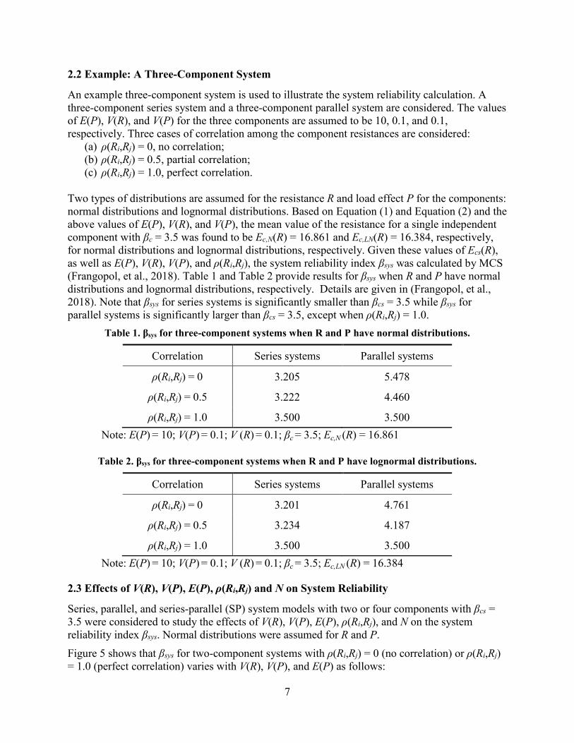
Two types of distributions are assumed for the resistance R and load effect P for the components: normal distributions and lognormal distributions. Based on Equation (1) and Equation (2) and the above values of E(P), V(R), and V(P), the mean value of the resistance for a single independent component with βc = 3.5 was found to be Ec,N(R) = 16.861 and Ec,LN(R) = 16.384, respectively, for normal distributions and lognormal distributions, respectively. Given these values of Ecs(R), as well as E(P), V(R), V(P), and ρ(Ri,Rj), the system reliability index βsys was calculated by MCS (Frangopol, et al., 2018). Table 1 and Table 2 provide results for βsys when R and P have normal distributions and lognormal distributions, respectively. Details are given in (Frangopol, et al., 2018). Note that βsys for series systems is significantly smaller than βcs = 3.5 while βsys for parallel systems is significantly larger than βcs = 3.5, except when ρ(Ri,Rj) = 1.0.
Table 1. βsys for three-component systems when R and P have normal distributions.
Correlation Series systems Parallel systems
ρ(Ri,Rj) = 0 3.205 5.478
ρ(Ri,Rj) = 0.5 3.222 4.460
ρ(Ri,Rj) = 1.0 3.500 3.500Note: E(P) = 10; V(P) = 0.1; V (R) = 0.1; βc = 3.5; Ec,N (R) = 16.861
Table 2. βsys for three-component systems when R and P have lognormal distributions.
Correlation Series systems Parallel systems
ρ(Ri,Rj) = 0 3.201 4.761
ρ(Ri,Rj) = 0.5 3.234 4.187
ρ(Ri,Rj) = 1.0 3.500 3.500Note: E(P) = 10; V(P) = 0.1; V (R) = 0.1; βc = 3.5; Ec,LN (R) = 16.384
2.3 Effects of V(R), V(P), E(P), ρ(Ri,Rj) and N on System Reliability
Series, parallel, and series-parallel (SP) system models with two or four components with βcs = 3.5 were considered to study the effects of V(R), V(P), E(P), ρ(Ri,Rj), and N on the system reliability index βsys. Normal distributions were assumed for R and P.Figure 5 shows that βsys for two-component systems with ρ(Ri,Rj) = 0 (no correlation) or ρ(Ri,Rj) = 1.0 (perfect correlation) varies with V(R), V(P), and E(P) as follows:

8
(a) as V(R) increases, βsys for ρ(Ri,Rj) = 0 (no correlation) increases significantly for theparallel system while it decreases slightly for the series system;
(b) as V(P) increases, βsys for ρ(Ri,Rj) = 0 remains almost the same for the series system whileit decreases significantly for the parallel system;
(c) βsys is unaffected by change in the mean value of the load E(P) for both systems and forboth correlation cases;
(d) for ρ(Ri,Rj) = 1.0 (perfect correlation), βsys for both systems is equal to 3.5 and is unaffectedby changes in V(R), V(P), and E(P).
Figure 5. Graph. Effects of (a) V(R); (b) V(P); and (c) E(P) on βsys for two-component systems for cases of no correlation and perfect correlation among resistances.
βsys for four-component systems was also investigated. Three different four-component systems were considered: a series system (Figure 6(a)), a parallel system (Figure 6(b)), and a series-parallel (SP) system (Figure 6(c)).
Figure 6. Illustration. Four-component systems: (a) series system; (b) parallel system; and (c) series-parallel (SP) system.
9
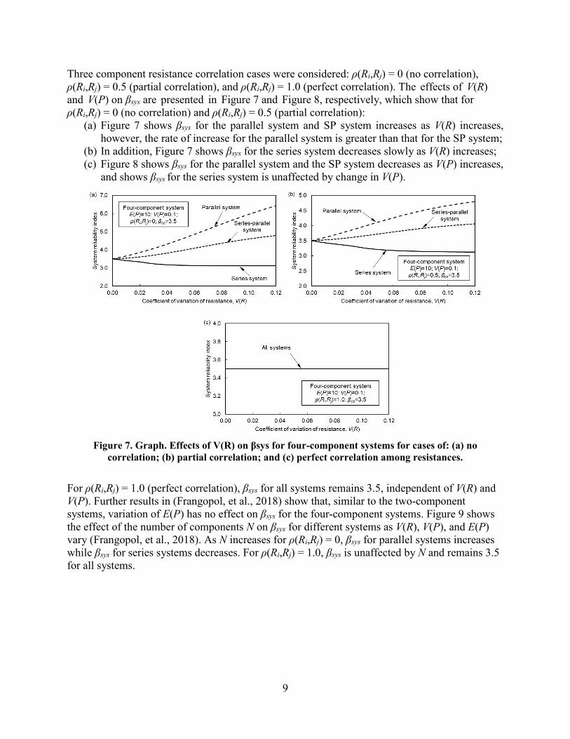
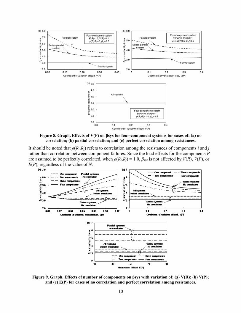
Three component resistance correlation cases were considered: ρ(Ri,Rj) = 0 (no correlation), ρ(Ri,Rj) = 0.5 (partial correlation), and ρ(Ri,Rj) = 1.0 (perfect correlation). The effects of V(R) and V(P) on βsys are presented in Figure 7 and Figure 8, respectively, which show that for ρ(Ri,Rj) = 0 (no correlation) and ρ(Ri,Rj) = 0.5 (partial correlation):
(a) Figure 7 shows βsys for the parallel system and SP system increases as V(R) increases,however, the rate of increase for the parallel system is greater than that for the SP system;
(b) In addition, Figure 7 shows βsys for the series system decreases slowly as V(R) increases;(c) Figure 8 shows βsys for the parallel system and the SP system decreases as V(P) increases,
and shows βsys for the series system is unaffected by change in V(P).
Figure 7. Graph. Effects of V(R) on βsys for four-component systems for cases of: (a) no correlation; (b) partial correlation; and (c) perfect correlation among resistances.
For ρ(Ri,Rj) = 1.0 (perfect correlation), βsys for all systems remains 3.5, independent of V(R) and V(P). Further results in (Frangopol, et al., 2018) show that, similar to the two-component systems, variation of E(P) has no effect on βsys for the four-component systems. Figure 9 shows the effect of the number of components N on βsys for different systems as V(R), V(P), and E(P) vary (Frangopol, et al., 2018). As N increases for ρ(Ri,Rj) = 0, βsys for parallel systems increases while βsys for series systems decreases. For ρ(Ri,Rj) = 1.0, βsys is unaffected by N and remains 3.5 for all systems.
10
Figure 8. Graph. Effects of V(P) on βsys for four-component systems for cases of: (a) no correlation; (b) partial correlation; and (c) perfect correlation among resistances.
It should be noted that ρ(Ri,Rj) refers to correlation among the resistances of components i and j rather than correlation between component failures. Since the load effects for the components P are assumed to be perfectly correlated, when ρ(Ri,Rj) = 1.0, βsys is not affected by V(R), V(P), or E(P), regardless of the value of N.
Figure 9. Graph. Effects of number of components on βsys with variation of: (a) V(R); (b) V(P); and (c) E(P) for cases of no correlation and perfect correlation among resistances.

11
2.4 Reliability of Systems with Many Equally Reliable Components
This subsection discusses βsys for systems with many components that have a target reliability index βcs = 3.5. Systems with up to 100 components (i.e., with N = 2, 3, 5, 10, 15, 20, 25, 50, or 100) are considered. As N increases, the computational effort to determine βsys increasesdramatically. Therefore, a representative case in which V(R) and V(P) are constant with V(R) =0.05 and V(P) = 0.3 is considered instead of studying various combinations of V(R) and V(P).Different series-parallel (SP) systems can be formed for an N-component system (see Figure 2 for example SP systems), and the following rules are used to define SP systems:
(a) if the SP system is composed of subsystems, with each typical subsystem having of mparallel components, and the typical subsystem is repeated n times in series, the SPsystem is defined to be an mp×ns SP system;
(b) if the SP system is composed of subsystems, with each typical subsystem having of mcomponents in series, and the typical subsystem is repeated n times in parallel, the SPsystem is defined to be an ms×np SP system.
In this study, SP systems with m equal to 5, 10 and 20 are investigated. With the reliability index for all components in the system βcs equal to 3.5, the system reliability index βsys for each system (with N = 2, 3, 5, 10, 15, 20, 25, 50, or 100) was calculated for:
(a) different system types (i.e., series, parallel, and SP);(b) three cases of correlation among component resistances: ρ(Ri,Rj) = 0 (no correlation),
ρ(Ri,Rj) = 0.5 (partial correlation), and ρ(Ri,Rj) = 1.0 (perfect correlation);(c) two types of distributions for R and P (i.e., normal or lognormal).
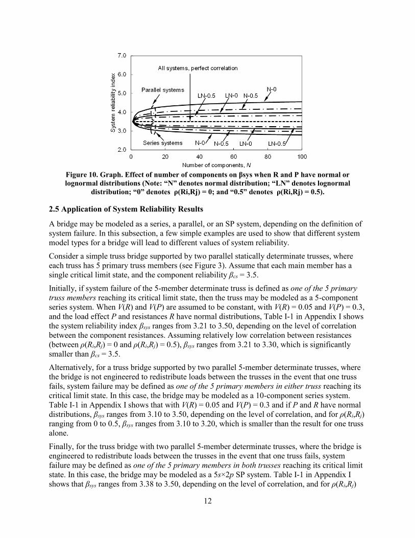
For the assumed values of V(R) = 0.05, V(P) = 0.3, and E(P) = 10, the mean resistance for each system component with βc = βcs = 3.5 was found to be Ecs,N(R) = Ec,N(R) = 21.132 and Ecs,LN(R) = Ec,LN(R) = 27.194, respectively, for normal and lognormal distributions, respectively. Given these values of Ecs(R), as well as the assumed values of E(P), V(R), V(P), ρ(Ri,Rj), and the distributions for R and P, the system reliability index βsys was calculated by MCS (Frangopol, et al., 2018). The results for βsys are given in Tables I-1, I-2, I-3, and I-4 in Appendix I, where Tables I-1 and I-2 give results when R and P have normal distributions, and Tables I-3 and I-4 give results whenR and P have lognormal distributions. Figure 10 shows selected results for the series systemsand the parallel systems as N increases. From the examination of the results presented in thesetables and Figure 10 it can be stated that:
(a) for ρ(Ri,Rj) = 0 (no correlation) and ρ(Ri,Rj) = 0.5 (partial correlation), it is observed thatfor the series systems and the set of mp×ns SP systems with the same number of parallelcomponents (i.e., the mp×ns SP systems with the same value of m), βsys decreases as thenumber of components N increases; however, for the parallel systems and the set ofms×np SP systems with the same number of series components (i.e., the ms×np SP withthe same value of m), βsys increases as the number of components N increases;
(b) for ρ(Ri,Rj) = 1.0 (perfect correlation), βsys is equal to 3.5 for the different types ofsystems with different number of components as expected;
(c) for the series systems, βsys for the lognormal distributions is greater than βsys for thenormal distributions; however, for the parallel systems, βsys for the lognormaldistributions is less than βsys for the normal distributions;
(d) as the correlation among component resistances (ρ(Ri,Rj)) increases, βsys decreases for theparallel systems while βsys increases for the series systems.
12
Figure 10. Graph. Effect of number of components on βsys when R and P have normal or lognormal distributions (Note: “N” denotes normal distribution; “LN” denotes lognormal
distribution; “0” denotes ρ(Ri,Rj) = 0; and “0.5” denotes ρ(Ri,Rj) = 0.5).
2.5 Application of System Reliability Results
A bridge may be modeled as a series, a parallel, or an SP system, depending on the definition of system failure. In this subsection, a few simple examples are used to show that different system model types for a bridge will lead to different values of system reliability.Consider a simple truss bridge supported by two parallel statically determinate trusses, where each truss has 5 primary truss members (see Figure 3). Assume that each main member has a single critical limit state, and the component reliability βcs = 3.5.Initially, if system failure of the 5-member determinate truss is defined as one of the 5 primary truss members reaching its critical limit state, then the truss may be modeled as a 5-component series system. When V(R) and V(P) are assumed to be constant, with V(R) = 0.05 and V(P) = 0.3, and the load effect P and resistances R have normal distributions, Table I-1 in Appendix I shows the system reliability index βsys ranges from 3.21 to 3.50, depending on the level of correlation between the component resistances. Assuming relatively low correlation between resistances (between ρ(Ri,Rj) = 0 and ρ(Ri,Rj) = 0.5), βsys ranges from 3.21 to 3.30, which is significantly smaller than βcs = 3.5. Alternatively, for a truss bridge supported by two parallel 5-member determinate trusses, where the bridge is not engineered to redistribute loads between the trusses in the event that one truss fails, system failure may be defined as one of the 5 primary members in either truss reaching its critical limit state. In this case, the bridge may be modeled as a 10-component series system. Table I-1 in Appendix I shows that with V(R) = 0.05 and V(P) = 0.3 and if P and R have normal distributions, βsys ranges from 3.10 to 3.50, depending on the level of correlation, and for ρ(Ri,Rj) ranging from 0 to 0.5, βsys ranges from 3.10 to 3.20, which is smaller than the result for one truss alone. Finally, for the truss bridge with two parallel 5-member determinate trusses, where the bridge is engineered to redistribute loads between the trusses in the event that one truss fails, system failure may be defined as one of the 5 primary members in both trusses reaching its critical limit state. In this case, the bridge may be modeled as a 5s×2p SP system. Table I-1 in Appendix I shows that βsys ranges from 3.38 to 3.50, depending on the level of correlation, and for ρ(Ri,Rj)
13
ranging from 0 to 0.5, βsys ranges from 3.38 to 3.39, which is larger than the result for one truss alone. Practically speaking, it is likely that an actual truss bridge would have far more than 5 members. For a 25-member truss modeled as a 25-component series system, Table I-2 in Appendix I shows that βsys ranges from 2.97 to 3.50, depending on the level of correlation, and for ρ(Ri,Rj) ranging from 0 to 0.5, βsys ranges from 2.97 to 3.10, significantly smaller than βcs = 3.5.For a truss bridge supported by two parallel 25-member determinate trusses, where the bridge is not engineered to redistribute loads between the trusses if one truss fails, the bridge may be modeled as a 50-component series system. Table I-2 in Appendix I shows that βsys ranges from 2.88 to 3.50, depending on the level of correlation, and for ρ(Ri,Rj) ranging from 0 to 0.5, βsys ranges from 2.88 to 3.04, again, significantly smaller than βcs = 3.5.In summary, for these various examples of determinate truss bridges, the system reliability index βsys may be far below the component reliability index for each member in the system βcs = 3.5. In such cases, a redundancy factor should be included into the component-based limit-state design equations to increase the system reliability (as described in Section 3 of this report).As another example bridge system, consider a steel girder bridge with 4 parallel girders, numbered from 1 to 4 (girders 1 and 4 are exterior girders and girders 2 and 3 refers to interior girders). Three different system models, as shown in Figure 4 can be considered, based on the definition of the girder bridge system failure:
(a) series model: the system fails if any girder reaches a critical limit state;(b) parallel model: the system fails if all girders reach a critical limit state;(c) SP model: the system fails if any two adjacent girders reach a critical limit state
simultaneously, which is a 2p×3s SP system model.For the series model of the 4-girder bridge, Table I-1 in Appendix I shows that with normal distributions and V(R) = 0.05 and V(P) = 0.3, βsys ranges from 3.25 to 3.50, depending on the level of correlation, and for ρ(Ri,Rj) ranging from 0 to 0.5, βsys ranges from 3.25 to 3.31, significantly smaller than βcs = 3.5. For the parallel model of the 4-girder bridge, Table I-1 in Appendix I shows that βsys ranges from 3.97 to 3.50, depending on the level of correlation, and for ρ(Ri,Rj) ranging from 0 to 0.5, βsys ranges from 3.97 to 3.80, significantly larger than βcs = 3.5. For the 2p×3s SP system model of the 4-girder bridge, Table I-1 in Appendix I shows that βsys ranges from 3.59 to 3.50, depending on the level of correlation, and for ρ(Ri,Rj) ranging from 0 to 0.5, βsys ranges from 3.59 to 3.53, which is larger than but within 3% of βcs = 3.5. In summary, for these various examples of a parallel girder bridge, the system reliability index βsys for the parallel and SP models is greater than the component reliability index for each member in the system βcs = 3.5. For the series system model, βsys is less than βcs.
14
3. Reliability-Based Redundancy Factors This section discusses the proposed reliability-based redundancy factor. The effects of several parameters on this redundancy factor are presented. Values of the redundancy factor for N-component systems are presented. Simple examples that apply the redundancy factor results are discussed. Use of the redundancy factor within a typical component-based limit-state design equation from the AASHTO LRFD bridge design specifications (AASHTO, 2016) is shown.
3.1 Definition of Redundancy Factor
Consider a single component with random resistance R and random load effect P. Given the mean value of the load E(P), the coefficients of variation V(R) and V(P), and the component reliability index βc = 3.5, the mean value of the single component resistance Ec(R) can be determined as discussed in Section 2. If R and P both have normal distributions, or both have lognormal distributions, Ec(R) can be calculated from Equation (1) or Equation (2), respectively. This value of Ec(R) is used as the reference value for comparison with the mean value of the resistance of the components in a system Ecs(R), to determine the reliability-based redundancy factor, denoted as ηR, for the system. For a system of N equally-reliable components, different system types (i.e., series, parallel, and SP) can be considered. Given the values of E(P), V(R), V(P), ρ(Ri,Rj), the distribution type for R and P, and the target system reliability index βsys, assumed to be 3.5, the mean value of the resistance of each component in the system Ecs(R) can be calculated as described in (Frangopol, et al., 2018). After obtaining Ecs(R) for βsys = 3.5, and the mean single component resistance Ec(R) for βc = 3.5, the redundancy factor ηR is calculated as the ratio of Ecs(R) to Ec(R).As Ecs(R) for βsys = 3.5 is calculated, the reliability index of each component in the system, βcs corresponding to βsys = 3.5, can be calculated as well. In general, βcs for a given βsys will not equal βsys or βc, and for the results in this section (Section 3), βcs is understood to be the reliability index of each component in the system required to have the target system reliability index βsys. In the calculations presented in Section 2, the reliability index of each component in the system βcs was set equal to the single component reliability index (βc = 3.5), and the corresponding system reliability index βsys was calculated.
3.2 Example: A Three-Component System
A simple example of the redundancy factor calculation is as follows. Three-component series systems and three-component parallel systems are considered. The values of E(P), V(R), and V(P) associated with the three components are assumed to be 10, 0.1, and 0.1, respectively. Three cases of correlation among the component resistances are considered: ρ(Ri,Rj) = 0 (no correlation), ρ(Ri,Rj) = 0.5 (partial correlation), and ρ(Ri,Rj) = 1.0 (perfect correlation).Both normal distributions and lognormal distributions are considered for R and P. Based on Equation (1) and Equation (2) and the above values of E(P), V(R), and V(P), the mean value of the single component resistance for βc = 3.5 is found to be Ec,N(R) = 16.861 and Ec,LN(R) = 16.384, respectively, for normal distributions and lognormal distributions, respectively. For βsys = 3.5, the mean value of the resistance of each component in the system Ecs(R) was calculated as described in (Frangopol, et al., 2018). ηR, is the ratio of Ecs(R) to Ec(R).Table 3 and Table 4 provide the results for Ecs(R), ηR, and βcs when R and P have normal

15
distributions and lognormal distributions, respectively. Further details are given in (Frangopol, et al., 2018). For ρ(Ri,Rj) = 0 (no correlation) and ρ(Ri,Rj) = 0.5 (partial correlation), Table 3 and Table 4 show that:
(a) the redundancy factor ηR for a series system is greater than 1.0, which indicates that the mean resistance required for each component in a series system is greater than that needed for a single component; the associated component reliability index βcs is greater than 3.5;
(b) ηR for a parallel system is less than 1.0, which indicates that the mean resistance required for each component in a parallel system is less than that needed for a single component; the associated βcs is less than 3.5.
For ρ(Ri,Rj) = 1.0 (perfect correlation case), ηR is 1.0, and βcs is 3.5. Comparing Table 3 with Table 4 shows that for ρ(Ri,Rj) = 0 and ρ(Ri,Rj) = 0.5, the difference in ηR for the normal and lognormal distributions is less than 6%.Table 3. Ecs(R), ηR, and βcs for three-component systems when R and P have normal distributions.
CorrelationSeries systems Parallel systems
Ecs(R) ηR βcs Ecs(R) ηR βcs
ρ(Ri,Rj) = 0 17.685 1.049 3.78 13.684 0.812 2.17
ρ(Ri,Rj) = 0.5 17.651 1.047 3.77 14.817 0.879 2.69
ρ(Ri,Rj) = 1.0 16.861 1.000 3.50 16.861 1.000 3.50Note: E(P) = 10; V(P) = 0.1; V (R) = 0.1; βc = 3.5; βsys = 3.5; Ec,N (R) = 16.861
Table 4. Ecs(R), ηR, and βcs for three-component systems when R and P have lognormal distributions.
CorrelationSeries systems Parallel systems
Ecs(R) ηR βcs Ecs(R) ηR βcs
ρ(Ri,Rj) = 0 17.945 1.040 3.78 14.092 0.860 2.43
ρ(Ri,Rj) = 0.5 16.985 1.037 3.76 14.969 0.914 2.86
ρ(Ri,Rj) = 1.0 16.384 1.000 3.50 16.384 1.000 3.50Note: E(P) = 10; V(P) = 0.1; V (R) = 0.1; βc = 3.5; βsys = 3.5; Ec,LN (R) = 16.384
3.3 Effects of V(R), V(P), E(P) and N on Redundancy Factor
Series, parallel, and SP system models with βsys of 3.5 and with two or four components were investigated to study the effects of V(R), V(P), E(P), ρ(Ri,Rj), and N on the redundancy factor ηR. Normal distributions for R and P were assumed. Figure 11 shows that the redundancy factor ηR for two-component systems with ρ(Ri,Rj) = 0 or ρ(Ri,Rj) = 1.0 varies with V(R), V(P), and E(P) as follows:
(a) as V(R) increases, ηR for ρ(Ri,Rj) = 0 (no correlation) increases for the series system while

16
it decreases significantly for the parallel system; (b) as V(P) increases, ηR for ρ(Ri,Rj) = 0 (no correlation) increases for both systems, but
increases more significantly for the parallel system; (c) ηR is unaffected by change in the mean value of the load E(P) for both systems and for
both correlation cases.(d) For ρ(Ri,Rj) = 1.0 (perfect correlation), ηR is 1.0, and is unaffected by V(R), V(P), and
E(P).
Figure 11. Graph. Effects of: (a) V(R); (b) V(P); and (c) E(P) on ηR for two-component systems.
These observations can be understood by considering the effects of V(R) and V(P) on the mean single component resistance Ec(R) and on the mean value of the resistance of each component in the system Ecs(R) as follows (see Figure 12):
(a) as V(R) or V(P) increases, Ec(R) and Ecs(R) increase for both correlation cases and for both the series system and the parallel system;
(b) for ρ(Ri,Rj) = 0 (no correlation) for the series system, the increase in Ecs(R) from an increase in V(R) or V(P) is more significant than the increase in Ec(R); therefore, ηR = Ecs(R) / Ec(R) increases as V(R) or V(P) increases;
(c) for ρ(Ri,Rj) = 0 (no correlation) for the parallel system, the increase of Ecs(R) from an increase in V(R) is less significant than the increase in Ec(R); therefore, ηR decreases as V(R) increases;
(d) for ρ(Ri,Rj) = 1.0 (perfect correlation) for both the series system and the parallel system, Ecs(R) = Ec(R) over the range of V(R) and V(P); therefore, ηR = 1.000 and V(R) and V(P) have no effect on the redundancy factor.
17
Figure 12. Graph. Effects of: (a) V(R); and (b) V(P) on Ec(R) and Ecs(R) for two-component systems.
ηR for four-component systems was also investigated. Three different four-component systems (series, parallel, and series-parallel (SP) systems) are shown in Figure 6. Three correlation cases were considered: ρ(Ri,Rj) = 0 (no correlation), ρ(Ri,Rj) = 0.5 (partial correlation), and ρ(Ri,Rj) = 1.0 (perfect correlation). The effects of V(R) and V(P) on ηR are presented in Figure 13 and Figure 14, respectively.Figure 13 shows that as V(R) increases for ρ(Ri,Rj) = 0 (no correlation) and ρ(Ri,Rj) = 0.5 (partial correlation), ηR values for the series system increase while ηR values for both the parallel and SP systems decrease. As the correlation increases, the sensitivity of ηR to changes in V(R) decreases. Figure 14 shows that as V(P) increases for ρ(Ri,Rj) = 0 and ρ(Ri,Rj) = 0.5, ηR increases for the series, parallel, and SP systems. For ρ(Ri,Rj) = 1.0 (perfect correlation), ηR for all systems remains 1.0, independent of V(R) and V(P). Further results given in (Frangopol, et al., 2018) show that, similar to the two-component systems, variation of E(P) has no effect on ηR for the four-component systems.Figure 15 shows the effects of the number of components N on ηR for different systems as V(R), V(P), and E(P) vary. As N increases for ρ(Ri,Rj) = 0 (no correlation), it is observed that ηR for series systems increases while ηR for parallel systems decreases. For ρ(Ri,Rj) = 1.0 (perfect correlation), ηR = 1.000 for all systems.
18
Figure 13. Graph. Effects of V(R) on ηR for four-component systems for cases of: (a) no correlation; (b) partial correlation; and (c) perfect correlation among resistances.
Figure 14. Graph. Effects of V(P) on ηR for four-component systems for cases of: (a) no correlation; (b) partial correlation; and (c) perfect correlation among resistances.

19
Figure 15. Graph. Effects of number of components on ηR with variation of: (a) V(R); (b) V(P); and (c) E(P) for cases of no correlation and perfect correlation among resistances.
3.4 Redundancy Factor for Systems with Many Equally Reliable Components
This subsection discusses ηR for systems with a target system reliability index βsys = 3.5. Systems with up to 100 components (i.e., with N = 2, 3, 5, 10, 15, 20, 25, 50, or 100) are considered. As N increases, the required computational effort to determine ηR increases dramatically. Therefore, V(R) and V(P) are constant with V(R) = 0.05 and V(P) = 0.3.Series, parallel, and various SP systems were studied, with the SP systems formed using the rules described in Section 2. Three correlation cases were considered: ρ(Ri,Rj) = 0 (no correlation), ρ(Ri,Rj) = 0.5 (partial correlation), and ρ(Ri,Rj) = 1.0 (perfect correlation). Normal and lognormal distributions for R and P are considered. E(P) was assumed to be 10.For the assumed values of V(R) = 0.05, V(P) = 0.3, and E(P) = 10, and with the component reliability index βc = 3.5, the mean value of the single component resistance Ec(R) was found to be Ec,N (R) = 21.132 and Ec,LN (R) = 27.194, respectively, for normal and lognormal distributions, respectively. For βsys = 3.5, the mean value of the resistance of each component in the system Ecs(R) was calculated (Frangopol, et al., 2018) and ηR was determined as the ratio of Ecs(R) to Ec(R) for each system (with N = 2, 3, 5, 10, 15, 20, 25, 50, or 100). The results are given in Appendix II, in Table II-1 through Table II-6 for normal distributions and Table II-7 through Table II-12 for lognormal distributions.It is observed from Table II-1 through Table II-12 in Appendix II:
(a) for the series systems and mp×ns SP systems with the same number of parallel components (i.e., m is the same), ηR increases as the number of components increases; however, for the parallel systems and ms×np SP systems with the same number of series components (i.e., m is the same), ηR decreases as the number of components increases;
(b) for the same number of components and system model type, ηR values for the normal
20
distributions and ηR values for the lognormal distributions are relatively close, indicating the effect of distribution type is not very significant;
(c) for ρ(Ri,Rj) = 1.0 (perfect correlation), ηR = 1.000 for all systems.
Figure 16 shows the variation of βcs and ηR for series and parallel systems as N increases, where:(a) as N increases, βcs and ηR increase for series systems, while βcs and ηR decrease for
parallel systems;(b) for series systems, βcs for normal distributions are larger than βcs for lognormal
distributions for ρ(Ri,Rj) = 0 and ρ(Ri,Rj) = 0.5; however, for parallel systems, βcs for normal distributions are smaller than βcs for lognormal distributions for ρ(Ri,Rj) = 0 and ρ(Ri,Rj) = 0.5;
(c) the effect of distribution type (i.e., normal versus lognormal) on ηR is not very significant;(d) for ρ(Ri,Rj) = 1.0 (perfect correlation), βcs =3.5 and ηR = 1.000 for all systems.
Figure 16. Graph. The effects of number of components on: (a) βcs; and (b) ηR (Note: “N” denotes normal distribution; “LN” denotes lognormal distribution; “0” denotes ρ(Ri,Rj) = 0; “0.5” denotes
ρ(Ri,Rj) = 0.5; V(R) = 0.05; V(P) = 0.3; E(P) = 10; and βc
3.5 Application of Redundancy Factor Results
As noted earlier, a bridge may be modeled as a series, a parallel, or an SP system, depending on the definition of system failure. In this subsection, a few simple examples are used to show that using different system model types for a bridge will lead to different values of the redundancy factor ηR needed to maintain a system reliability index βsys = 3.5.
Consider the truss bridge supported by two parallel statically determinate trusses, discussed in

21
Section 2, where each truss has 5 primary truss members (see Figure 3). Assume that each primary member has a single critical limit state, and βsys is intended to be 3.5.
Initially, if system failure of the 5-member determinate truss is defined as one of the 5 primary truss members reaching its critical limit state, then the truss may be modeled as a 5-component series system. When V(R) and V(P) are assumed to be constant, with V(R) = 0.05 and V(P) = 0.3, and the load effect P and resistances R have normal distributions, Tables II-1, II-3, II-5 show the redundancy factor ηR ranges from 1.047 to 1.000, depending on the level of correlation between the component resistances. Assuming relatively low correlation between resistances (between ρ(Ri,Rj) = 0 and ρ(Ri,Rj) = 0.5), ηR ranges from 1.047 to 1.037. Tables II-7, II-9, II-11 show ηR results when P and R have lognormal distributions, where ηR ranges from 1.051 to 1.037 for ρ(Ri,Rj) between 0 and 0.5.Alternatively, for the truss bridge supported by two parallel 5-member determinate trusses, where the bridge is not engineered to redistribute loads between the trusses, system failure may be defined as one of the 5 primary members in either truss reaching its critical limit state. In this case, the bridge may be modeled as a 10-component series system. Tables II-1, II-3, II-5 show that with V(R) = 0.05 and V(P) = 0.3 and when P and R have normal distributions, ηR ranges from 1.064 to 1.000, depending on the level of correlation, and for ρ(Ri,Rj) between 0 and 0.5, ηR ranges from 1.064 to 1.050. Tables II-7, II-9, II-11 show ηR results when P and R have lognormal distributions, where ηR ranges from 1.070 to 1.052 for ρ(Ri,Rj) between 0 and 0.5.Finally, for the truss bridge with two parallel 5-member determinate trusses, where the bridge is engineered to redistribute loads between the trusses in the event that one truss fails, system failure may be defined as one of the 5 primary members in both trusses reaching its critical limit state. In this case, the bridge may be modeled as a 5sx2p SP system. Tables II-1, II-3, II-5 show that for normal distributions and V(R) = 0.05 and V(P) = 0.3, ηR ranges from 1.019 to 1.000, depending on the level of correlation, and for ρ(Ri,Rj) between 0 and 0.5, ηR ranges from 1.019 to 1.018. Tables II-7, II-9, II-11 show that for lognormal distributions, ηR ranges from 1.028 to 1.023 for ρ(Ri,Rj) between 0 and 0.5.As noted in Section 2 it is likely that an actual truss bridge would have far more than 5 members. For the 25-member truss modeled as a 25-component series system, Tables II-2, II-4, and II-6 show that for normal distributions, ηR ranges from 1.088 to 1.000, depending on the level of correlation, and for ρ(Ri,Rj) between 0 and 0.5, ηR ranges from 1.088 to 1.066.For the truss bridge supported by two parallel 25-member determinate trusses, where the bridge is not engineered to redistribute loads between the trusses, the bridge may be modeled as a 50-component series system. Tables II-2, II-4, and II-6 show that for normal distributions, ηR ranges from 1.104 to 1.000, depending on the level of correlation, and for ρ(Ri,Rj) between 0 and 0.5, ηR ranges from 1.104 to 1.077. Tables II-8, II-10, and II-12 show that for lognormal distributions, ηR ranges from 1.107 to 1.077 for ρ(Ri,Rj) between 0 and 0.5.In summary, for these various examples of determinate truss bridges, different values of the redundancy factor ηR are needed to maintain a system reliability index βsys = 3.5. The values are as large as 1.070 for the truss bridge with two parallel 5-member trusses, and as large as 1.107 for the truss bridge with two parallel 25-member trusses.The steel girder bridge with 4 parallel girders, numbered from 1 to 4 (girders 1 and 4 are exterior girders and girders 2 and 3 refers to interior girders), discussed in Section 2, is also considered as an example. The three different system models shown in Figure 4 were considered:
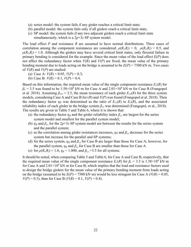
22
(a) series model: the system fails if any girder reaches a critical limit state;(b) parallel model: the system fails only if all girders reach a critical limit state;(c) SP model: the system fails if any two adjacent girders reach a critical limit state
simultaneously, which is a 2p×3s SP system model.The load effect P and resistance R are assumed to have normal distributions. Three cases of correlation among the component resistances are considered: ρ(Ri,Rj) = 0, ρ(Ri,Rj) = 0.5, and ρ(Ri,Rj) = 1.0. Although the girders may have several critical limit states, only flexural failure in primary bending is considered for the example. Since the mean value of the load effect E(P) does not affect the redundancy factor when V(R) and V(P) are fixed, the mean value of the primary bending moment due to loads acting on the bridge is assumed to be E(P) = 7500 kN·m. Two cases of V(R) and V(P) are studied:
(a) Case A: V(R) = 0.05, V(P) = 0.3;(b) Case B: V(R) = 0.1, V(P) = 0.4.
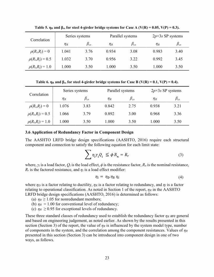
Based on this information, the required mean value of the single component resistance Ec(R) for βc = 3.5 was found to be 1.58×10⁴ kN·m for Case A and 2.01×10⁴ kN·m for Case B (Frangopol et al. 2018). Assuming βsys = 3.5, the mean resistance of each girder Ecs(R) for the three system models, considering Case A and Case B for (R) and V(P) was found (Frangopol et al. 2018). Then the redundancy factor ηR was determined as the ratio of Ecs(R) to Ec(R), and the associated reliability index of each girder in the bridge system βcs was determined (Frangopol, et al., 2018). The results are given in Table 5 and Table 6, where it is shown that:
(a) the redundancy factor ηR and the girder reliability index βcs are largest for the series system model and smallest for the parallel system model;
(b) ηR and βcs for the 2p×3s SP system model are between the results for the series system and the parallel system;
(c) as the correlation among girder resistances increases, ηR and βcs decrease for the series system but increase for the parallel and SP systems;
(d) for the series system, ηR and βcs for Case B are larger than those for Case A; however, for the parallel system, ηR and βcs for Case B are smaller than those for Case A
(e) for ρ(Ri,Rj) = 1.0, ηR = 1.000, and βcs =3.5 for all systems.
It should be noted, when comparing Table 5 and Table 6, for Case A and Case B, respectively, that the required mean value of the single component resistance Ec(R) for βc = 3.5 is 1.58×10⁴ kN·m for Case A and 2.01×10⁴ kN·m for Case B, which implies that the load and resistance factors used to design the bridge girders for the mean value of the primary bending moment from loads acting on the bridge (assumed to be E(P) = 7500 kN·m) would be less stringent for Case A (V(R) = 0.05, V(P) = 0.3), than for Case B (V(R) = 0.1, V(P) = 0.4).
23
Table 5. ηR and βcs for steel 4-girder bridge systems for Case A (V(R) = 0.05, V(P) = 0.3).
CorrelationSeries systems Parallel systems 2p×3s SP systems
ηR βcs ηR βcs ηR βcs
ρ(Ri,Rj) = 0 1.041 3.76 0.934 3.08 0.983 3.40
ρ(Ri,Rj) = 0.5 1.032 3.70 0.956 3.22 0.992 3.45
ρ(Ri,Rj) = 1.0 1.000 3.50 1.000 3.50 1.000 3.50
Table 6. ηR and βcs for steel 4-girder bridge systems for Case B (V(R) = 0.1, V(P) = 0.4).
CorrelationSeries systems Parallel systems 2p×3s SP systems
ηR βcs ηR βcs ηR βcs
ρ(Ri,Rj) = 0 1.076 3.83 0.842 2.75 0.938 3.21
ρ(Ri,Rj) = 0.5 1.066 3.79 0.892 3.00 0.968 3.36
ρ(Ri,Rj) = 1.0 1.000 3.50 1.000 3.50 1.000 3.50
3.6 Application of Redundancy Factor in Component Design
The AASHTO LRFD bridge design specifications (AASHTO, 2016) require each structural component and connection to satisfy the following equation for each limit state:
where, γi is a load factor, Qi is the load effect, ϕ is the resistance factor, Rn is the nominal resistance, Rr is the factored resistance, and ηi is a load effect modifier:
(4)
where ηD is a factor relating to ductility, ηR is a factor relating to redundancy, and ηl is a factor relating to operational classification. As noted in Section 1 of the report, ηR in the AASHTO LRFD bridge design specifications (AASHTO, 2016) is determined as follows:
(a) ηR ≥ 1.05 for nonredundant members;(b) ηR = 1.00 for conventional level of redundancy;(c) ηR ≥ 0.95 for exceptional levels of redundancy.
These three standard classes of redundancy used to establish the redundancy factor ηR are general and based on engineering judgement, as noted earlier. As shown by the results presented in this section (Section 3) of the report, the value of ηR is influenced by the system model type, number of components in the system, and the correlation among the component resistances. Values of ηR presented in this section (Section 3) can be introduced into component design in one of two ways, as follows.
(3)
24
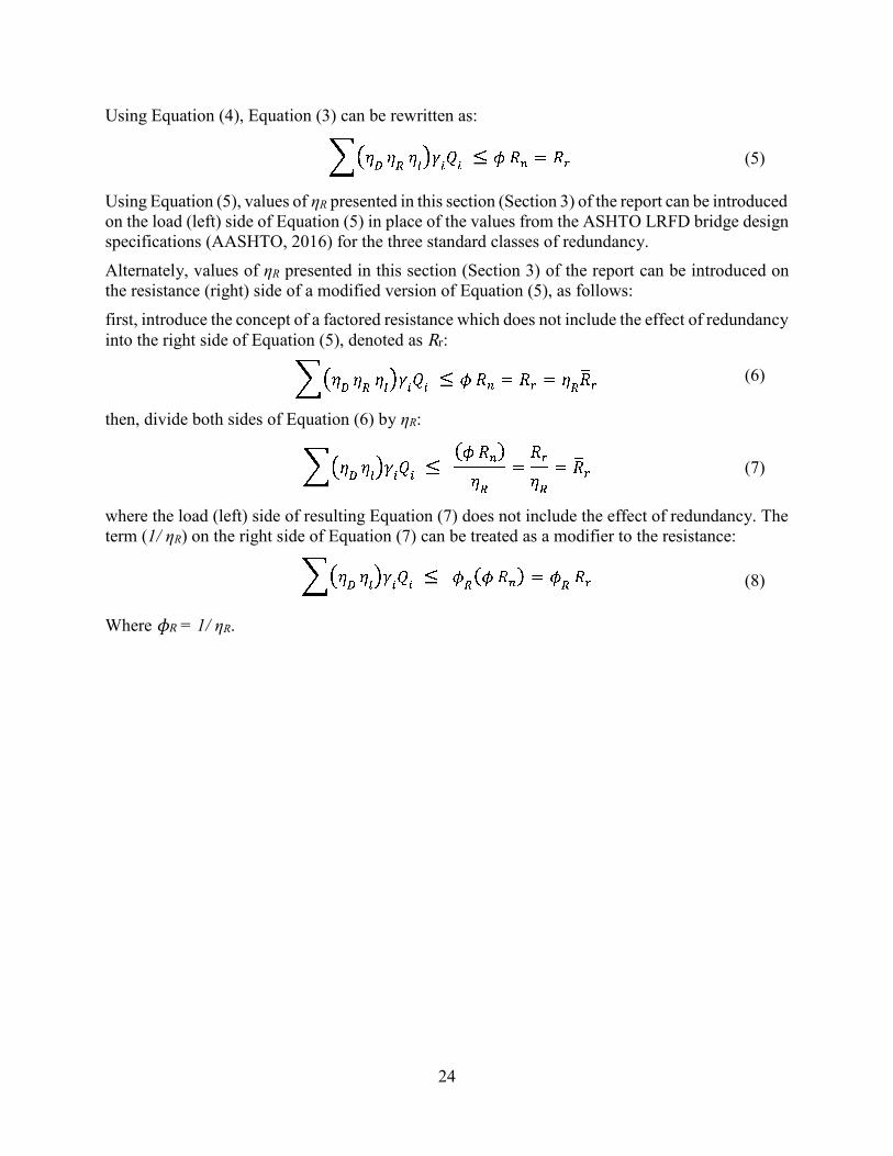
Using Equation (4), Equation (3) can be rewritten as:
(5)
Using Equation (5), values of ηR presented in this section (Section 3) of the report can be introduced on the load (left) side of Equation (5) in place of the values from the ASHTO LRFD bridge design specifications (AASHTO, 2016) for the three standard classes of redundancy.Alternately, values of ηR presented in this section (Section 3) of the report can be introduced on the resistance (right) side of a modified version of Equation (5), as follows: first, introduce the concept of a factored resistance which does not include the effect of redundancy into the right side of Equation (5), denoted as R� r:
(6)
then, divide both sides of Equation (6) by ηR:
(7)
where the load (left) side of resulting Equation (7) does not include the effect of redundancy. The term (1/ ηR) on the right side of Equation (7) can be treated as a modifier to the resistance:
(8)
Where ɸR = 1/ ηR.

25
4. Reliability-Based Redundancy Factors for Ductile and Brittle SystemsThis section presents reliability-based redundancy factors ηR for systems with components that have ductile or brittle post-failure behavior. Redundancy factors for systems consisting of both ductile and brittle components (denoted “mixed system”) are also presented. Systems with up to four components are considered. A ductile system has only ductile components, and the component resistance is constant and not reduced after failure (i.e., after the critical limit state is reached). This ductile behavior is elastic-perfectly-plastic. A brittle system has only brittle components, and the component resistance decreases to zero after failure. Mixed systems include both types of components.
4.1 Redundancy Factor for Ductile Systems
Consider a single component when both R and P have normal distributions with V(R), V(P), and E(P) equal to 0.05, 0.3, and 10, respectively. From Equation (1), the mean resistance of Ec(R) is found to be 21.132 to make the component reliability index βc = 3.5. Then, consider a system consisting of two ductile components. Series and parallel systems can be considered. Since failure of any component in the series system corresponds to system failure, the system reliability of the series system βsys is not affected by the component post-failure behavior. Consequently, the redundancy factor ηR for a series system is also independent of the component post-failure behavior. Therefore, the study of ηR in this section focuses on parallel and SP systems.For a two-component ductile parallel system, the resistances of the two components are denoted as R1 and R2. The total load acting on the system is 2P with the load distributed to each component equal to P. The ductile components of the system have constant resistance after failure. Therefore, the limit state equation for the two-component ductile parallel system is:
(9)
Based on this limit state equation, and with βsys = 3.5 and the values of V(R), V(P), E(P), and Ec(R) as given above, the mean value of the resistance of each component in the system Ecs(R) to maintain a system reliability index βsys = 3.5 and the corresponding βcs was calculated as described in (Frangopol, et al., 2018). ηR is the ratio of Ecs(R) to Ec(R). Three cases of correlation among the resistances were considered: ρ(Ri,Rj) = 0 (no correlation), ρ(Ri,Rj) = 0.5 (partial correlation), and ρ(Ri,Rj) = 1.0 (perfect correlation). The corresponding results are Ecs(R) = 20.810, 20.950, and 21.132, respectively; ηR = 0.985, 0.991, and 1.0, respectively; and βcs = 3.40, 3.45, and 3.50, respectively.These results can be compared with those from Tables II-1, II-3, II-5 in Appendix II, which are Ecs(R) = 20.310, 20.590, and 21.124, respectively; and ηR = 0.961, 0.974, and 1.0. These comparisons show that for parallel two-component systems, considering ductile component behavior with load redistribution leads to larger values of ηR compared to the previous results (except for the case of ρ(Ri,Rj) = 1.0), when load redistribution after a component fails (i.e., reaches a critical limit state) was not considered. For a three-component ductile parallel system, the resistances of the components are denoted R1, R2, and R3. The total load acting on the system is 3P. Two types of probability distribution, normal and lognormal, are considered. For the values of V(R), V(P), and E(P) given above, and for βc = 3.5, the mean single component resistance Ec(R) = 21.132, when R and P have normal
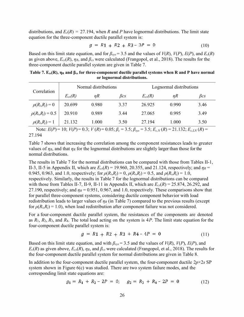
26
distributions, and Ec(R) = 27.194, when R and P have lognormal distributions. The limit state equation for the three-component ductile parallel system is:
(10)
Based on this limit state equation, and for βsys = 3.5 and the values of V(R), V(P), E(P), and Ec(R) as given above, Ecs(R), ηR, and βcs were calculated (Frangopol, et al., 2018). The results for the three-component ductile parallel system are given in Table 7.Table 7. Ecs(R), ηR and βcs for three-component ductile parallel systems when R and P have normal
or lognormal distributions.
CorrelationNormal distributions Lognormal distributions
Ecs(R) ηR βcs Ecs(R) ηR βcs
ρ(Ri,Rj) = 0 20.699 0.980 3.37 26.925 0.990 3.46
ρ(Ri,Rj) = 0.5 20.910 0.989 3.44 27.065 0.995 3.49
ρ(Ri,Rj) = 1 21.132 1.000 3.50 27.194 1.000 3.50Note: E(P) = 10; V(P) = 0.3; V (R) = 0.05; βc = 3.5; βsys = 3.5; Ec,N (R) = 21.132; Ec,LN (R) =
27.194Table 7 shows that increasing the correlation among the component resistances leads to greater values of ηR, and that ηR for the lognormal distributions are slightly larger than those for the normal distributions.The results in Table 7 for the normal distributions can be compared with those from Tables II-1, II-3, II-5 in Appendix II, which are Ecs(R) = 19.960, 20.355, and 21.124, respectively; and ηR =0.945, 0.963, and 1.0, respectively; for ρ(Ri,Rj) = 0, ρ(Ri,Rj) = 0.5, and ρ(Ri,Rj) = 1.0,respectively. Similarly, the results in Table 7 for the lognormal distributions can be comparedwith those from Tables II-7, II-9, II-11 in Appendix II, which are Ecs(R) = 25.874, 26.292, and27.190, respectively; and ηR = 0.951, 0.967, and 1.0, respectively. These comparisons show thatfor parallel three-component systems, considering ductile component behavior with loadredistribution leads to larger values of ηR (in Table 7) compared to the previous results (exceptfor ρ(Ri,Rj) = 1.0), when load redistribution after component failure was not considered.For a four-component ductile parallel system, the resistances of the components are denoted as R1, R2, R3, and R4. The total load acting on the system is 4P. The limit state equation for the four-component ductile parallel system is:
(11)
Based on this limit state equation, and with βsys = 3.5 and the values of V(R), V(P), E(P), and Ec(R) as given above, Ecs(R), ηR, and βcs were calculated (Frangopol, et al., 2018). The results for the four-component ductile parallel system for normal distributions are given in Table 8.In addition to the four-component ductile parallel system, the four-component ductile 2p×2s SP system shown in Figure 6(c) was studied. There are two system failure modes, and the corresponding limit state equations are:
(12)

27
Based on these limit state equations, Ecs(R), ηR, and βcs were calculated (Frangopol, et al., 2018). The results for the four-component ductile 2p×2s SP systems for normal distributions are given in Table 8.
Table 8. Ecs(R), ηR and βcs for four-component ductile systems when R and P have normal distributions.
CorrelationParallel systems 2p×2s SP systems
Ecs(R) ηR βcs Ecs(R) ηR βcs
ρ(Ri,Rj) = 0 20.660 0.978 3.36 21.160 1.001 3.51
ρ(Ri,Rj) = 0.5 20.893 0.989 3.43 21.231 1.005 3.53
ρ(Ri,Rj) = 1.0 21.132 1.000 3.50 21.132 1.000 3.50Note: E(P) = 10; V(P) = 0.3; V (R) = 0.05; βc = 3.5; βsys = 3.5; Ec,N (R) = 21.132
Table 8 shows that increasing the correlation among the resistances of components leads to larger values of ηR. Also, Table 8 shows that for the no correlation and partial correlation cases, Ecs(R) and ηR for the 2p×2s SP systems are higher than those for the parallel systems. Also, for the 2p×2s SP systems, ηR is close to 1.0 regardless of the correlation.The results of the four-component ductile parallel systems in Table 8 can be compared with those from Tables II-1, II-3, II-5 in Appendix II, which are Ecs(R) = 19.737, 20.202, and 21.124, respectively; and ηR = 0.934, 0.956, and 1.0, respectively. These comparisons show that for parallel four-component systems, considering ductile component behavior with load redistribution leads to larger values of ηR (in Table 8) compared to the previous results (except for ρ(Ri,Rj) = 1.0), when load redistribution after component failure was not considered.
4.2 Redundancy Factor for Brittle Systems
Since a brittle component will not resist load after failure, the load for that component will distribute to other components that have not failed. Therefore, for a brittle system, different failure sequences lead to different load distributions on the components, and thus to different system failure modes. To illustrate the redundancy factor for brittle systems, two-, three-, and four-component systems are considered.Consider a two-component parallel system. If both components are brittle, two different failure modes can be anticipated:
(a) Mode I, the failure of component 1 followed by component 2;(b) Mode II, the failure of component 2 followed by component 1.
28
Therefore, the two-component brittle parallel system failure can be evaluated by using the SP system model shown in Figure 17, where the parallel subsystem on the left represents Mode I and the parallel subsystem on the right represents Mode II. The two-component system has resistances R1 and R2, and total applied load of 2P. The sets of limit state equations for each of the two failure modes are given by Equation (13) and Equation (14):
(13)
(14)
Limit state equations g1 and g3 (Equation (13)) represent Mode I, where component 1 carries half the applied load (P = ½(2P)) at failure (limit state equation g1), and has zero resistance after failure, so that the total applied load (2P) is carried by component 2 after component 1 fails (limit state equation g3). Similarly, limit state equations g2 and g4 (Equation (14)) represent Mode II.
Figure 17. Illustration. Failure modes of two-component brittle parallel system.
With R and load P normally distributed, and with V(R), V(P), and E(P) assumed to be 0.05, 0.3, and 10, respectively, the mean single component resistance Ec(R) is 21.132 for βc = 3.5. Based on Equation (13) and Equation (14), βsys = 3.5, and these values of V(R), V(P), E(P), and Ec(R), the mean value of the resistance of each component in the system Ecs(R) and the corresponding βcs was calculated as described in (Frangopol, et al., 2018). ηR was determined as the ratio of Ecs(R) to Ec(R). Three cases of component resistance correlation were considered: ρ(Ri,Rj) = 0, ρ(Ri,Rj) = 0.5, and ρ(Ri,Rj) = 1.0. The corresponding results are Ecs(R) = 21.585, 21.481, and 21.132, respectively; ηR = 1.021, 1.017, and 1.0, respectively; and βcs = 3.63, 3.60, and 3.50, respectively. Note that ηR for the brittle parallel system decreases as the ρ(Ri,Rj) increases.These results can be compared with those for a two-component ductile parallel system, which are Ecs(R) = 20.810, 20.950, and 21.132, respectively; ηR = 0.985, 0.991, and 1.0, respectively. The comparison indicates that a two-component brittle parallel system requires significantly larger Ecs(R) and ηR (except for ρ(Ri,Rj) = 1) to maintain a system reliability index βsys = 3.5.
In addition, these results can be compared with those from Tables II-1, II-3, II-5 in Appendix II, which are Ecs(R) = 20.310, 20.590, and 21.124, respectively; and ηR = 0.961, 0.974, and 1.0, respectively, These comparisons show that for parallel two-component systems, considering brittle component behavior with load redistribution leads to larger values of ηR compared to the previous results, when load redistribution after component failure was not considered.For a three-component brittle parallel system, with resistances R1, R2, and R3, and total applied load of 3P, six failure modes can be anticipated, and the system failure can be evaluated by using the SP system model shown in Figure 18, where each parallel subsystem represents a failure mode. The sets of limit state equations for each of the six failure modes are:
(15)
(16)
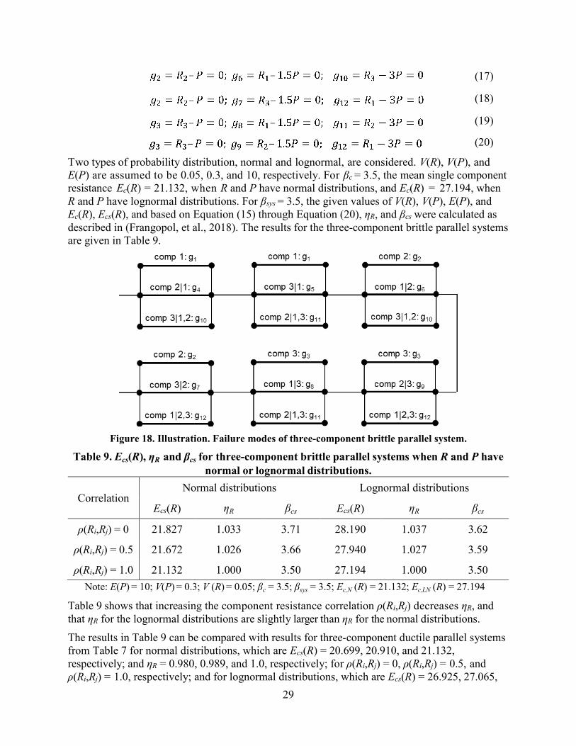
29
(17)
(18)
(19)
(20)
Two types of probability distribution, normal and lognormal, are considered. V(R), V(P), and E(P) are assumed to be 0.05, 0.3, and 10, respectively. For βc = 3.5, the mean single component resistance Ec(R) = 21.132, when R and P have normal distributions, and Ec(R) = 27.194, when R and P have lognormal distributions. For βsys = 3.5, the given values of V(R), V(P), E(P), and Ec(R), Ecs(R), and based on Equation (15) through Equation (20), ηR, and βcs were calculated as described in (Frangopol, et al., 2018). The results for the three-component brittle parallel systems are given in Table 9.
Figure 18. Illustration. Failure modes of three-component brittle parallel system.
Table 9. Ecs(R), ηR and βcs for three-component brittle parallel systems when R and P have normal or lognormal distributions.
CorrelationNormal distributions Lognormal distributions
Ecs(R) ηR βcs Ecs(R) ηR βcs
ρ(Ri,Rj) = 0 21.827 1.033 3.71 28.190 1.037 3.62
ρ(Ri,Rj) = 0.5 21.672 1.026 3.66 27.940 1.027 3.59
ρ(Ri,Rj) = 1.0 21.132 1.000 3.50 27.194 1.000 3.50Note: E(P) = 10; V(P) = 0.3; V (R) = 0.05; βc = 3.5; βsys = 3.5; Ec,N (R) = 21.132; Ec,LN (R) = 27.194
Table 9 shows that increasing the component resistance correlation ρ(Ri,Rj) decreases ηR, and that ηR for the lognormal distributions are slightly larger than ηR for the normal distributions.The results in Table 9 can be compared with results for three-component ductile parallel systems from Table 7 for normal distributions, which are Ecs(R) = 20.699, 20.910, and 21.132, respectively; and ηR = 0.980, 0.989, and 1.0, respectively; for ρ(Ri,Rj) = 0, ρ(Ri,Rj) = 0.5, and ρ(Ri,Rj) = 1.0, respectively; and for lognormal distributions, which are Ecs(R) = 26.925, 27.065,
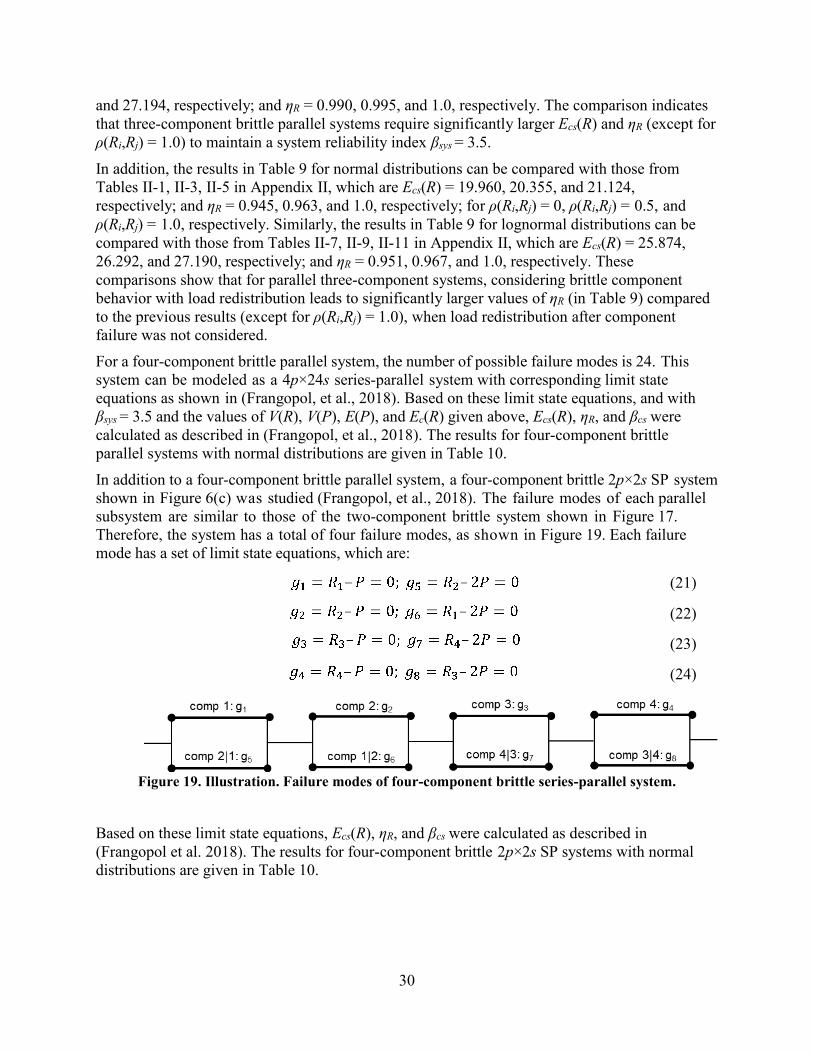
30
and 27.194, respectively; and ηR = 0.990, 0.995, and 1.0, respectively. The comparison indicates that three-component brittle parallel systems require significantly larger Ecs(R) and ηR (except for ρ(Ri,Rj) = 1.0) to maintain a system reliability index βsys = 3.5.
In addition, the results in Table 9 for normal distributions can be compared with those from Tables II-1, II-3, II-5 in Appendix II, which are Ecs(R) = 19.960, 20.355, and 21.124, respectively; and ηR = 0.945, 0.963, and 1.0, respectively; for ρ(Ri,Rj) = 0, ρ(Ri,Rj) = 0.5, and ρ(Ri,Rj) = 1.0, respectively. Similarly, the results in Table 9 for lognormal distributions can be compared with those from Tables II-7, II-9, II-11 in Appendix II, which are Ecs(R) = 25.874, 26.292, and 27.190, respectively; and ηR = 0.951, 0.967, and 1.0, respectively. These comparisons show that for parallel three-component systems, considering brittle component behavior with load redistribution leads to significantly larger values of ηR (in Table 9) compared to the previous results (except for ρ(Ri,Rj) = 1.0), when load redistribution after component failure was not considered.For a four-component brittle parallel system, the number of possible failure modes is 24. This system can be modeled as a 4p×24s series-parallel system with corresponding limit state equations as shown in (Frangopol, et al., 2018). Based on these limit state equations, and with βsys = 3.5 and the values of V(R), V(P), E(P), and Ec(R) given above, Ecs(R), ηR, and βcs were calculated as described in (Frangopol, et al., 2018). The results for four-component brittle parallel systems with normal distributions are given in Table 10.In addition to a four-component brittle parallel system, a four-component brittle 2p×2s SP system shown in Figure 6(c) was studied (Frangopol, et al., 2018). The failure modes of each parallel subsystem are similar to those of the two-component brittle system shown in Figure 17. Therefore, the system has a total of four failure modes, as shown in Figure 19. Each failure mode has a set of limit state equations, which are:
(21)
(22)
(23)
(24)
Figure 19. Illustration. Failure modes of four-component brittle series-parallel system.
Based on these limit state equations, Ecs(R), ηR, and βcs were calculated as described in (Frangopol et al. 2018). The results for four-component brittle 2p×2s SP systems with normal distributions are given in Table 10.
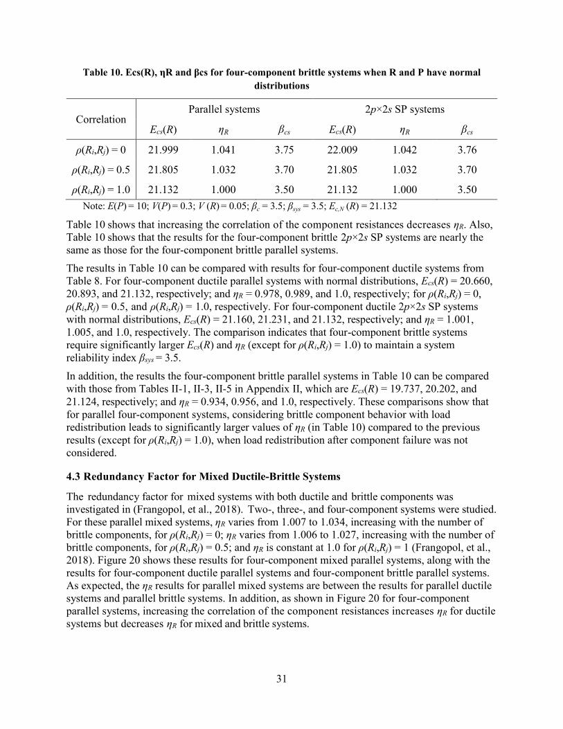
31
Table 10. Ecs(R), ηR and βcs for four-component brittle systems when R and P have normal distributions
CorrelationParallel systems 2p×2s SP systems
Ecs(R) ηR βcs Ecs(R) ηR βcs
ρ(Ri,Rj) = 0 21.999 1.041 3.75 22.009 1.042 3.76
ρ(Ri,Rj) = 0.5 21.805 1.032 3.70 21.805 1.032 3.70
ρ(Ri,Rj) = 1.0 21.132 1.000 3.50 21.132 1.000 3.50Note: E(P) = 10; V(P) = 0.3; V (R) = 0.05; βc = 3.5; βsys = 3.5; Ec,N (R) = 21.132
Table 10 shows that increasing the correlation of the component resistances decreases ηR. Also, Table 10 shows that the results for the four-component brittle 2p×2s SP systems are nearly the same as those for the four-component brittle parallel systems. The results in Table 10 can be compared with results for four-component ductile systems from Table 8. For four-component ductile parallel systems with normal distributions, Ecs(R) = 20.660, 20.893, and 21.132, respectively; and ηR = 0.978, 0.989, and 1.0, respectively; for ρ(Ri,Rj) = 0, ρ(Ri,Rj) = 0.5, and ρ(Ri,Rj) = 1.0, respectively. For four-component ductile 2p×2s SP systems with normal distributions, Ecs(R) = 21.160, 21.231, and 21.132, respectively; and ηR = 1.001, 1.005, and 1.0, respectively. The comparison indicates that four-component brittle systems require significantly larger Ecs(R) and ηR (except for ρ(Ri,Rj) = 1.0) to maintain a system reliability index βsys = 3.5.
In addition, the results the four-component brittle parallel systems in Table 10 can be compared with those from Tables II-1, II-3, II-5 in Appendix II, which are Ecs(R) = 19.737, 20.202, and 21.124, respectively; and ηR = 0.934, 0.956, and 1.0, respectively. These comparisons show that for parallel four-component systems, considering brittle component behavior with load redistribution leads to significantly larger values of ηR (in Table 10) compared to the previous results (except for ρ(Ri,Rj) = 1.0), when load redistribution after component failure was not considered.
4.3 Redundancy Factor for Mixed Ductile-Brittle Systems
The redundancy factor for mixed systems with both ductile and brittle components was investigated in (Frangopol, et al., 2018). Two-, three-, and four-component systems were studied. For these parallel mixed systems, ηR varies from 1.007 to 1.034, increasing with the number of brittle components, for ρ(Ri,Rj) = 0; ηR varies from 1.006 to 1.027, increasing with the number of brittle components, for ρ(Ri,Rj) = 0.5; and ηR is constant at 1.0 for ρ(Ri,Rj) = 1 (Frangopol, et al., 2018). Figure 20 shows these results for four-component mixed parallel systems, along with the results for four-component ductile parallel systems and four-component brittle parallel systems. As expected, the ηR results for parallel mixed systems are between the results for parallel ductile systems and parallel brittle systems. In addition, as shown in Figure 20 for four-component parallel systems, increasing the correlation of the component resistances increases ηR for ductile systems but decreases ηR for mixed and brittle systems.

32
Figure 20. Graph. Effects of number of brittle components on redundancy factor for four-component mixed parallel systems.
In addition, four-component mixed 2p×2s SP systems with various combinations of ductile and brittle components were studied (Frangopol, et al., 2018). For these four-component mixed 2p×2s SP systems, ηR varies from 1.015 and 1.034, increasing with the number of brittle components, for ρ(Ri,Rj) = 0; ηR varies from 1.014 and 1.027, increasing with the number of brittle components, for ρ(Ri,Rj) = 0.5; and ηR is constant at 1.0 for ρ(Ri,Rj) = 1 (Frangopol, et al., 2018). These results are similar to those for four-component mixed parallel systems.
4.4 Summary of Redundancy Factors for Ductile and Brittle Systems
Comparing the results for ductile systems and brittle systems with up to four components (Table 7 to Table 10), and comparing these results with the results from Section 3 (Appendix II), where load redistribution after component failure was not considered, the following observations are made:
(a) ηR for a ductile parallel system is at most 1.0 while ηR for a brittle parallel system is at least 1.0;
(b) increasing the component resistance correlation ρ(Ri,Rj) increases ηR for ductile systems but decreases ηR for mixed and brittle systems;
(c) comparing similar ductile and brittle systems, brittle systems require significantly larger ηR (except for cases with ρ(Ri,Rj) = 1.0) to maintain a system reliability index βsys = 3.5.
(d) for both ductile and brittle parallel systems, ηR values when R and P have lognormal distributions are slightly larger than those for normal distributions;
(e) for ductile systems, ηR for the four-component 2p×2s SP system is higher than ηR for the four-component parallel system; while, for brittle systems, ηR for the four-component 2p×2s SP and four-component parallel systems are almost the same;
(f) compared to the ηR values from Section 3 (given in Appendix II), where load redistribution after component failure was not considered, considering ductile component behavior with load redistribution leads to larger values of ηR (in Tables 7 and 8) except for ρ(Ri,Rj) = 1.0, while considering brittle component behavior with load redistribution leads to significantly larger values of ηR (in Table 9 and 10) except when ρ(Ri,Rj) = 1.0.
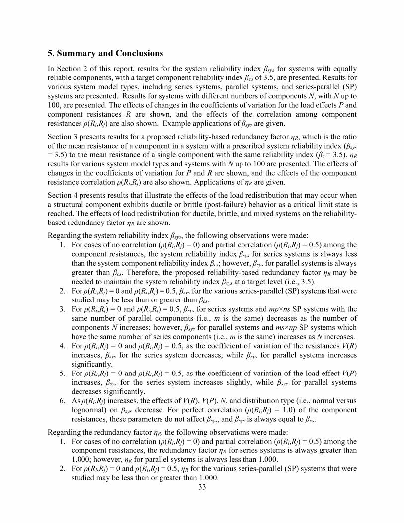
33
5. Summary and ConclusionsIn Section 2 of this report, results for the system reliability index βsys for systems with equally reliable components, with a target component reliability index βcs of 3.5, are presented. Results for various system model types, including series systems, parallel systems, and series-parallel (SP) systems are presented. Results for systems with different numbers of components N, with N up to 100, are presented. The effects of changes in the coefficients of variation for the load effects P and component resistances R are shown, and the effects of the correlation among component resistances ρ(Ri,Rj) are also shown. Example applications of βsys are given.
Section 3 presents results for a proposed reliability-based redundancy factor ηR, which is the ratio of the mean resistance of a component in a system with a prescribed system reliability index (βsys = 3.5) to the mean resistance of a single component with the same reliability index (βc = 3.5). ηR results for various system model types and systems with N up to 100 are presented. The effects of changes in the coefficients of variation for P and R are shown, and the effects of the component resistance correlation ρ(Ri,Rj) are also shown. Applications of ηR are given.Section 4 presents results that illustrate the effects of the load redistribution that may occur when a structural component exhibits ductile or brittle (post-failure) behavior as a critical limit state is reached. The effects of load redistribution for ductile, brittle, and mixed systems on the reliability-based redundancy factor ηR are shown.Regarding the system reliability index βsys, the following observations were made:
1. For cases of no correlation (ρ(Ri,Rj) = 0) and partial correlation (ρ(Ri,Rj) = 0.5) among the component resistances, the system reliability index βsys for series systems is always less than the system component reliability index βcs; however, βsys for parallel systems is always greater than βcs. Therefore, the proposed reliability-based redundancy factor ηR may be needed to maintain the system reliability index βsys at a target level (i.e., 3.5).
2. For ρ(Ri,Rj) = 0 and ρ(Ri,Rj) = 0.5, βsys for the various series-parallel (SP) systems that were studied may be less than or greater than βcs.
3. For ρ(Ri,Rj) = 0 and ρ(Ri,Rj) = 0.5, βsys for series systems and mp×ns SP systems with the same number of parallel components (i.e., m is the same) decreases as the number of components N increases; however, βsys for parallel systems and ms×np SP systems which have the same number of series components (i.e., m is the same) increases as N increases.
4. For ρ(Ri,Rj) = 0 and ρ(Ri,Rj) = 0.5, as the coefficient of variation of the resistances V(R) increases, βsys for the series system decreases, while βsys for parallel systems increases significantly.
5. For ρ(Ri,Rj) = 0 and ρ(Ri,Rj) = 0.5, as the coefficient of variation of the load effect V(P) increases, βsys for the series system increases slightly, while βsys for parallel systems decreases significantly.
6. As ρ(Ri,Rj) increases, the effects of V(R), V(P), N, and distribution type (i.e., normal versus lognormal) on βsys decrease. For perfect correlation (ρ(Ri,Rj) = 1.0) of the component resistances, these parameters do not affect βsys, and βsys is always equal to βcs.
Regarding the redundancy factor ηR, the following observations were made:1. For cases of no correlation (ρ(Ri,Rj) = 0) and partial correlation (ρ(Ri,Rj) = 0.5) among the
component resistances, the redundancy factor ηR for series systems is always greater than 1.000; however, ηR for parallel systems is always less than 1.000.
2. For ρ(Ri,Rj) = 0 and ρ(Ri,Rj) = 0.5, ηR for the various series-parallel (SP) systems that were studied may be less than or greater than 1.000.
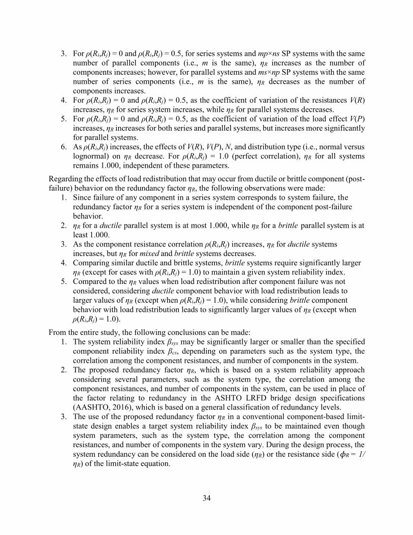
34
3. For ρ(Ri,Rj) = 0 and ρ(Ri,Rj) = 0.5, for series systems and mp×ns SP systems with the same number of parallel components (i.e., m is the same), ηR increases as the number of components increases; however, for parallel systems and ms×np SP systems with the same number of series components (i.e., m is the same), ηR decreases as the number of components increases.
4. For ρ(Ri,Rj) = 0 and ρ(Ri,Rj) = 0.5, as the coefficient of variation of the resistances V(R) increases, ηR for series system increases, while ηR for parallel systems decreases.
5. For ρ(Ri,Rj) = 0 and ρ(Ri,Rj) = 0.5, as the coefficient of variation of the load effect V(P) increases, ηR increases for both series and parallel systems, but increases more significantly for parallel systems.
6. As ρ(Ri,Rj) increases, the effects of V(R), V(P), N, and distribution type (i.e., normal versus lognormal) on ηR decrease. For ρ(Ri,Rj) = 1.0 (perfect correlation), ηR for all systems remains 1.000, independent of these parameters.
Regarding the effects of load redistribution that may occur from ductile or brittle component (post-failure) behavior on the redundancy factor ηR, the following observations were made:
1. Since failure of any component in a series system corresponds to system failure, the redundancy factor ηR for a series system is independent of the component post-failure behavior.
2. ηR for a ductile parallel system is at most 1.000, while ηR for a brittle parallel system is at least 1.000.
3. As the component resistance correlation ρ(Ri,Rj) increases, ηR for ductile systems increases, but ηR for mixed and brittle systems decreases.
4. Comparing similar ductile and brittle systems, brittle systems require significantly larger ηR (except for cases with ρ(Ri,Rj) = 1.0) to maintain a given system reliability index.
5. Compared to the ηR values when load redistribution after component failure was not considered, considering ductile component behavior with load redistribution leads to larger values of ηR (except when ρ(Ri,Rj) = 1.0), while considering brittle component behavior with load redistribution leads to significantly larger values of ηR (except when ρ(Ri,Rj) = 1.0).
From the entire study, the following conclusions can be made:1. The system reliability index βsys may be significantly larger or smaller than the specified
component reliability index βcs, depending on parameters such as the system type, the correlation among the component resistances, and number of components in the system.
2. The proposed redundancy factor ηR, which is based on a system reliability approach considering several parameters, such as the system type, the correlation among the component resistances, and number of components in the system, can be used in place of the factor relating to redundancy in the ASHTO LRFD bridge design specifications (AASHTO, 2016), which is based on a general classification of redundancy levels.
3. The use of the proposed redundancy factor ηR in a conventional component-based limit-state design enables a target system reliability index βsys to be maintained even though system parameters, such as the system type, the correlation among the component resistances, and number of components in the system vary. During the design process, the system redundancy can be considered on the load side (ηR) or the resistance side (ɸR = 1/ ηR) of the limit-state equation.

35
References
1. AASHTO. 2016. AASHTO LRFD Bridge Design Specifications. AASHTO LRFD Bridge Design Specifications, 7th Edition. Washington, DC : American Association of State Highway and Transportation Officials, 2016.
2. Frangopol, Dan M, Zhu, Benjin and Sabatino, Samantha. 2018. System Reliability in Special Steel and Concrete Bridge Systems: Identification of Redundancy Factor Modifiers. Bethlehem, PA : ATLSS Engineering Research Center, Lehigh University, 2018.

36
Appendix I. Reliability of Systems with Equally Reliable Components
Table I- 1. βsys for different systems with 1 ≤ N ≤ 20 for different correlation cases when R and P have normal distributions.
System ρ(Ri,Rj) = 0 ρ(Ri,Rj) = 0.5 ρ(Ri,Rj) = 1.0
1-component system 3.50 3.50 3.50
2-component system: Series system 3.368 3.393 3.50
2-component system: Parallel system 3.757 3.687 3.50
3-component system: Series system 3.293 3.338 3.50
3-component system: Parallel system 3.883 3.701 3.50
4-component system: Series system 3.245 3.305 3.50
4-component system: Parallel system 3.968 3.802 3.50
5-component system: Series system 3.207 3.302 3.50
5-component system: Parallel system 4.019 3.815 3.50
6-component system: 2p×3s SP system 3.590 3.532 3.50
10-component system: Series system 3.097 3.196 3.50
10-component system: Parallel system 4.156 3.904 3.50
10-component system: 5p×2s SP system 3.928 3.765 3.50
10-component system: 5s×2p SP system 3.376 3.385 3.50
15-component system: Series system 3.036 3.152 3.50
15-component system: Parallel system 4.248 4.028 3.50
15-component system: 5p×3s SP system 3.867 3.716 3.50
15-component system: 5s×3p SP system 3.455 3.432 3.50
20-component system: Series system 2.996 3.122 3.50
20-component system: Parallel system 4.298 4.043 3.50
20-component system: 5p×4s SP system 3.845 3.702 3.50
20-component system: 10p×2s SP system 4.100 3.871 3.50
20-component system: 5s×4p SP system 3.502 3.463 3.50
20-component system: 10s×2p SP system 3.244 3.286 3.50Note: E(P) = 10; V(P) = 0.3; V(R) = 0.05; βc = 3.5
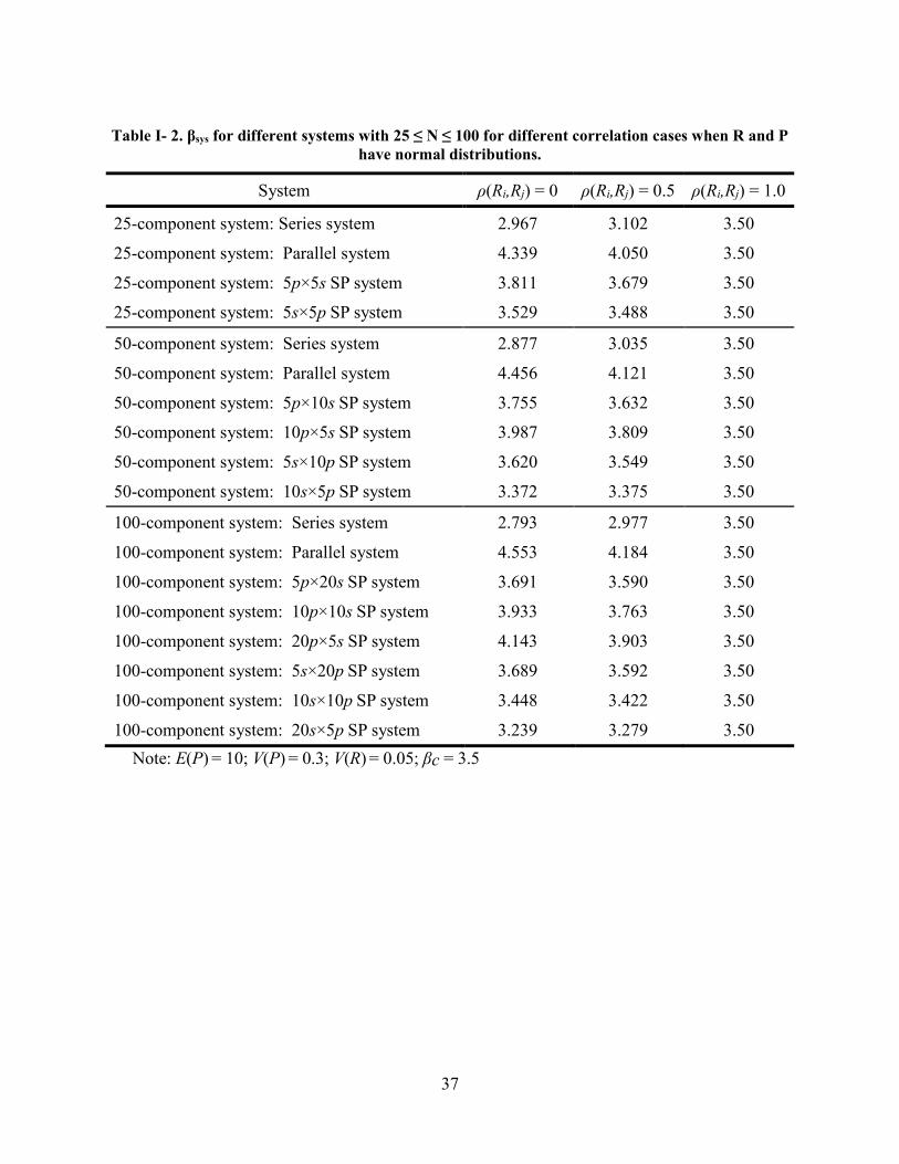
37
Table I- 2. βsys for different systems with 25 ≤ N ≤ 100 for different correlation cases when R and P have normal distributions.
System ρ(Ri,Rj) = 0 ρ(Ri,Rj) = 0.5 ρ(Ri,Rj) = 1.0
25-component system: Series system 2.967 3.102 3.50
25-component system: Parallel system 4.339 4.050 3.50
25-component system: 5p×5s SP system 3.811 3.679 3.50
25-component system: 5s×5p SP system 3.529 3.488 3.50
50-component system: Series system 2.877 3.035 3.50
50-component system: Parallel system 4.456 4.121 3.50
50-component system: 5p×10s SP system 3.755 3.632 3.50
50-component system: 10p×5s SP system 3.987 3.809 3.50
50-component system: 5s×10p SP system 3.620 3.549 3.50
50-component system: 10s×5p SP system 3.372 3.375 3.50
100-component system: Series system 2.793 2.977 3.50
100-component system: Parallel system 4.553 4.184 3.50
100-component system: 5p×20s SP system 3.691 3.590 3.50
100-component system: 10p×10s SP system 3.933 3.763 3.50
100-component system: 20p×5s SP system 4.143 3.903 3.50
100-component system: 5s×20p SP system 3.689 3.592 3.50
100-component system: 10s×10p SP system 3.448 3.422 3.50
100-component system: 20s×5p SP system 3.239 3.279 3.50Note: E(P) = 10; V(P) = 0.3; V(R) = 0.05; βc = 3.5
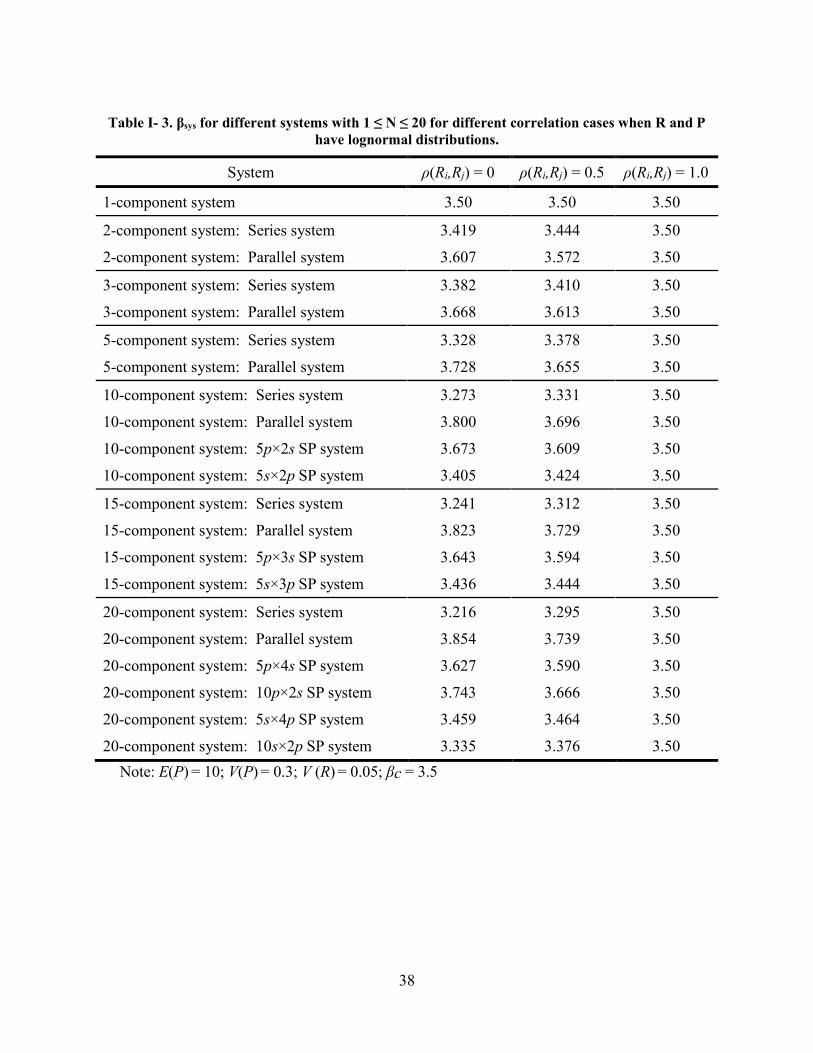
38
Table I- 3. βsys for different systems with 1 ≤ N ≤ 20 for different correlation cases when R and P have lognormal distributions.
System ρ(Ri,Rj) = 0 ρ(Ri,Rj) = 0.5 ρ(Ri,Rj) = 1.0
1-component system 3.50 3.50 3.50
2-component system: Series system 3.419 3.444 3.50
2-component system: Parallel system 3.607 3.572 3.50
3-component system: Series system 3.382 3.410 3.50
3-component system: Parallel system 3.668 3.613 3.50
5-component system: Series system 3.328 3.378 3.50
5-component system: Parallel system 3.728 3.655 3.50
10-component system: Series system 3.273 3.331 3.50
10-component system: Parallel system 3.800 3.696 3.50
10-component system: 5p×2s SP system 3.673 3.609 3.50
10-component system: 5s×2p SP system 3.405 3.424 3.50
15-component system: Series system 3.241 3.312 3.50
15-component system: Parallel system 3.823 3.729 3.50
15-component system: 5p×3s SP system 3.643 3.594 3.50
15-component system: 5s×3p SP system 3.436 3.444 3.50
20-component system: Series system 3.216 3.295 3.50
20-component system: Parallel system 3.854 3.739 3.50
20-component system: 5p×4s SP system 3.627 3.590 3.50
20-component system: 10p×2s SP system 3.743 3.666 3.50
20-component system: 5s×4p SP system 3.459 3.464 3.50
20-component system: 10s×2p SP system 3.335 3.376 3.50Note: E(P) = 10; V(P) = 0.3; V (R) = 0.05; βc = 3.5
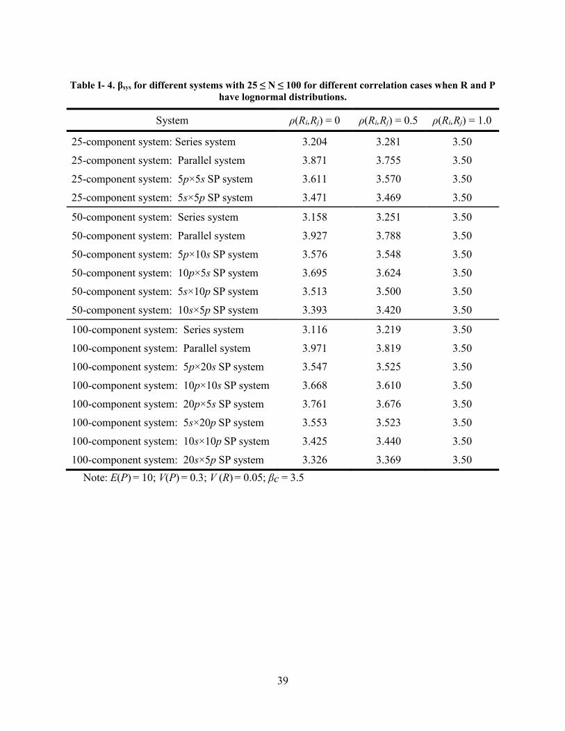
39
Table I- 4. βsys for different systems with 25 ≤ N ≤ 100 for different correlation cases when R and P have lognormal distributions.
System ρ(Ri,Rj) = 0 ρ(Ri,Rj) = 0.5 ρ(Ri,Rj) = 1.0
25-component system: Series system 3.204 3.281 3.50
25-component system: Parallel system 3.871 3.755 3.50
25-component system: 5p×5s SP system 3.611 3.570 3.50
25-component system: 5s×5p SP system 3.471 3.469 3.50
50-component system: Series system 3.158 3.251 3.50
50-component system: Parallel system 3.927 3.788 3.50
50-component system: 5p×10s SP system 3.576 3.548 3.50
50-component system: 10p×5s SP system 3.695 3.624 3.50
50-component system: 5s×10p SP system 3.513 3.500 3.50
50-component system: 10s×5p SP system 3.393 3.420 3.50
100-component system: Series system 3.116 3.219 3.50
100-component system: Parallel system 3.971 3.819 3.50
100-component system: 5p×20s SP system 3.547 3.525 3.50
100-component system: 10p×10s SP system 3.668 3.610 3.50
100-component system: 20p×5s SP system 3.761 3.676 3.50
100-component system: 5s×20p SP system 3.553 3.523 3.50
100-component system: 10s×10p SP system 3.425 3.440 3.50
100-component system: 20s×5p SP system 3.326 3.369 3.50Note: E(P) = 10; V(P) = 0.3; V (R) = 0.05; βc = 3.5
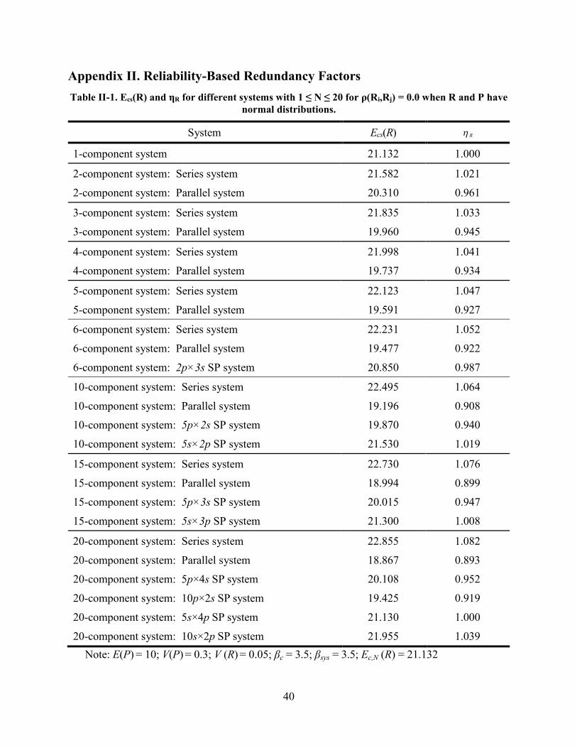
40
Appendix II. Reliability-Based Redundancy FactorsTable II-1. Ecs(R) and ηR for different systems with 1 ≤ N ≤ 20 for ρ(Ri,Rj) = 0.0 when R and P have
normal distributions.
System Ecs(R) h R
1-component system 21.132 1.000
2-component system: Series system 21.582 1.021
2-component system: Parallel system 20.310 0.961
3-component system: Series system 21.835 1.033
3-component system: Parallel system 19.960 0.945
4-component system: Series system 21.998 1.041
4-component system: Parallel system 19.737 0.934
5-component system: Series system 22.123 1.047
5-component system: Parallel system 19.591 0.927
6-component system: Series system 22.231 1.052
6-component system: Parallel system 19.477 0.922
6-component system: 2p×3s SP system 20.850 0.987
10-component system: Series system 22.495 1.064
10-component system: Parallel system 19.196 0.908
10-component system: 5p×2s SP system 19.870 0.940
10-component system: 5s×2p SP system 21.530 1.019
15-component system: Series system 22.730 1.076
15-component system: Parallel system 18.994 0.899
15-component system: 5p×3s SP system 20.015 0.947
15-component system: 5s×3p SP system 21.300 1.008
20-component system: Series system 22.855 1.082
20-component system: Parallel system 18.867 0.893
20-component system: 5p×4s SP system 20.108 0.952
20-component system: 10p×2s SP system 19.425 0.919
20-component system: 5s×4p SP system 21.130 1.000
20-component system: 10s×2p SP system 21.955 1.039Note: E(P) = 10; V(P) = 0.3; V (R) = 0.05; βc = 3.5; βsys = 3.5; Ec,N (R) = 21.132

41
Table II- 2. Ecs(R) and ηR for different systems with 25 ≤ N ≤ 100 for ρ(Ri,Rj) = 0 when R and P have normal distributions.
System Ecs(R) h R
25-component system: Series system 22.987 1.088
25-component system: Parallel system 18.773 0.888
25-component system: 5p×5s SP system 20.193 0.955
25-component system: 5s×5p SP system 21.030 0.995
50-component system: Series system 23.321 1.104
50-component system: Parallel system 18.510 0.876
50-component system: 5p×10s SP system 20.370 0.964
50-component system: 10p×5s SP system 19.682 0.931
50-component system: 5s×10p SP system 20.770 0.983
50-component system: 10s×5p SP system 21.540 1.019
100-component system: Series system 23.631 1.118
100-component system: Parallel system 18.306 0.866
100-component system: 5p×10s SP system 20.551 0.972
100-component system: 10p×10s SP system 19.846 0.939
100-component system: 20p×5s SP system 19.293 0.913
100-component system: 5s×20p SP system 20.550 0.972
100-component system: 10s×10p SP system 21.300 1.008
100-component system: 20s×5p SP system 21.980 1.040Note: E(P) = 10; V(P) = 0.3; V (R) = 0.05; βc = 3.5; βsys = 3.5; Ec,N (R) = 21.132

42
Table II- 3. Ecs(R) and ηR for different systems with 1 ≤ N ≤ 20 for ρ(Ri,Rj) = 0.5 when R and P have normal distributions.
System Ecs(R) h R
1-component system 21.132 1.000
2-component system: Series system 21.480 1.016
2-component system: Parallel system 20.590 0.974
3-component system: Series system 21.680 1.026
3-component system: Parallel system 20.355 0.963
4-component system: Series system 21.808 1.032
4-component system: Parallel system 20.202 0.956
5-component system: Series system 21.910 1.037
5-component system: Parallel system 20.080 0.950
6-component system: Series system 21.981 1.040
6-component system: Parallel system 20.000 0.946
6-component system: 2p×3s SP system 21.025 0.995
10-component system: Series system 22.190 1.050
10-component system: Parallel system 19.795 0.937
10-component system: 5p×2s SP system 20.309 0.961
10-component system: 5s×2p SP system 21.512 1.018
15-component system: Series system 22.360 1.058
15-component system: Parallel system 19.654 0.930
15-component system: 5p×3s SP system 20.425 0.967
15-component system: 5s×3p SP system 21.350 1.010
20-component system: Series system 22.453 1.063
20-component system: Parallel system 19.549 0.925
20-component system: 5p×4s SP system 20.490 0.970
20-component system: 10p×2s SP system 19.990 0.946
20-component system: 5s×4p SP system 21.245 1.005
20-component system: 10s×2p SP system 21.835 1.033Note: E(P) = 10; V(P) = 0.3; V (R) = 0.05; βc = 3.5; βsys = 3.5; Ec,N (R) = 21.132

43
Table II- 4. Ecs(R) and ηR for different systems with 25 ≤ N ≤ 100 for ρ(Ri,Rj) = 0.5 when R and P have normal distributions.
System Ecs(R) h R
25-component system: Series system 22.530 1.066
25-component system: Parallel system 19.481 0.922
25-component system: 5p×5s SP system 20.540 0.972
25-component system: 5s×5p SP system 21.175 1.002
50-component system: Series system 22.768 1.077
50-component system: Parallel system 19.277 0.912
50-component system: 5p×10s SP system 20.703 0.980
50-component system: 10p×5s SP system 20.190 0.955
50-component system: 5s×10p SP system 20.980 0.993
50-component system: 10s×5p SP system 21.545 1.020
100-component system: Series system 23.005 1.089
100-component system: Parallel system 19.124 0.905
100-component system: 5p×10s SP system 20.840 0.986
100-component system: 10p×10s SP system 20.305 0.961
100-component system: 20p×5s SP system 19.890 0.941
100-component system: 5s×20p SP system 20.840 0.986
100-component system: 10s×10p SP system 21.385 1.012
100-component system: 20s×5p SP system 21.880 1.035Note: E(P) = 10; V(P) = 0.3; V (R) = 0.05; βc = 3.5; βsys = 3.5; Ec,N (R) = 21.132

44
Table II- 5. Ecs(R) and ηR for different systems with 1 ≤ N ≤ 20 for ρ(Ri,Rj) = 1.0 when R and P have normal distributions.
System Ecs(R) h R
1-component system 21.132 1.000
2-component system: Series system 21.125 1.000
2-component system: Parallel system 21.124 1.000
3-component system: Series system 21.124 1.000
3-component system: Parallel system 21.124 1.000
4-component system: Series system 21.124 1.000
4-component system: Parallel system 21.124 1.000
5-component system: Series system 21.124 1.000
5-component system: Parallel system 21.124 1.000
6-component system: Series system 21.127 1.000
6-component system: Parallel system 21.127 1.000
6-component system: 2p×3s SP system 21.127 1.000
10-component system: Series system 21.131 1.000
10-component system: Parallel system 21.130 1.000
10-component system: 5p×2s SP system 21.130 1.000
10-component system: 5s×2p SP system 21.130 1.000
15-component system: Series system 21.131 1.000
15-component system: Parallel system 21.131 1.000
15-component system: 5p×3s SP system 21.131 1.000
15-component system: 5s×3p SP system 21.131 1.000
20-component system: Series system 21.132 1.000
20-component system: Parallel system 21.132 1.000
20-component system: 5p×4s SP system 21.132 1.000
20-component system: 10p×2s SP system 21.132 1.000
20-component system: 5s×4p SP system 21.132 1.000
20-component system: 10s×2p SP system 21.132 1.000Note: E(P) = 10; V(P) = 0.3; V (R) = 0.05; βc = 3.5; βsys = 3.5; Ec,N (R) = 21.132

45
Table II- 6. Ecs(R) and ηR for different systems with 25 ≤ N ≤ 100 for ρ(Ri,Rj) = 1.0 when R and P have normal distributions.
System Ecs(R) h R
25-component system: Series system 21.132 1.000
25-component system: Parallel system 21.132 1.000
25-component system: 5p×5s SP system 21.132 1.000
25-component system: 5s×5p SP system 21.132 1.000
50-component system: Series system 21.132 1.000
50-component system: Parallel system 21.132 1.000
50-component system: 5p×10s SP system 21.132 1.000
50-component system: 10p×5s SP system 21.132 1.000
50-component system: 5s×10p SP system 21.132 1.000
50-component system: 10s×5p SP system 21.132 1.000
100-component system: Series system 21.133 1.000
100-component system: Parallel system 21.133 1.000
100-component system: 5p×10s SP system 21.133 1.000
100-component system: 10p×10s SP system 21.133 1.000
100-component system: 20p×5s SP system 21.133 1.000
100-component system: 5s×20p SP system 21.133 1.000
100-component system: 10s×10p SP system 21.133 1.000
100-component system: 20s×5p SP system 21.133 1.000Note: E(P) = 10; V(P) = 0.3; V (R) = 0.05; βc = 3.5; βsys = 3.5; Ec,N (R) = 21.132

46
Table II- 7. Ecs(R) and ηR for different systems with 1 ≤ N ≤ 25 for ρ(Ri,Rj) = 0 when R and P have lognormal distributions.
System Ecs(R) h R
1-component system 27.194 1.000
2-component system: Series system 27.839 1.024
2-component system: Parallel system 26.292 0.967
3-component system: Series system 28.209 1.037
3-component system: Parallel system 25.874 0.951
5-component system: Series system 28.596 1.051
5-component system: Parallel system 25.441 0.935
10-component system: Series system 29.115 1.070
10-component system: Parallel system 24.922 0.916
10-component system: 5p×2s SP system 25.864 0.951
10-component system: 5s×2p SP system 27.960 1.028
15-component system: Series system 29.349 1.079
15-component system: Parallel system 24.674 0.907
15-component system: 5p×3s SP system 26.082 0.959
15-component system: 5s×3p SP system 27.710 1.019
20-component system: Series system 29.561 1.087
20-component system: Parallel system 24.501 0.901
20-component system: 5p×4s SP system 26.208 0.964
20-component system: 10p×2s SP system 25.286 0.930
20-component system: 5s×4p SP system 27.550 1.013
20-component system: 10s×2p SP system 28.600 1.052
25-component system: Series system 29.650 1.090
25-component system: Parallel system 24.368 0.896
25-component system: 5p×5s SP system 26.328 0.968
25-component system: 5s×5p SP system 27.390 1.007Note: E(P) = 10; V(P) = 0.3; V (R) = 0.05; βc = 3.5; βsys = 3.5; Ec,LN (R) = 27.194
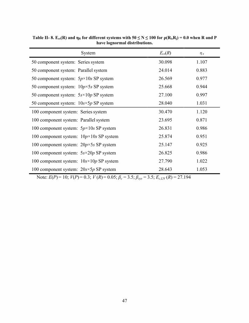
47
Table II- 8. Ecs(R) and ηR for different systems with 50 ≤ N ≤ 100 for ρ(Ri,Rj) = 0.0 when R and P have lognormal distributions.
System Ecs(R) h R
50 component system: Series system 30.098 1.107
50 component system: Parallel system 24.014 0.883
50 component system: 5p×10s SP system 26.569 0.977
50 component system: 10p×5s SP system 25.668 0.944
50 component system: 5s×10p SP system 27.100 0.997
50 component system: 10s×5p SP system 28.040 1.031
100 component system: Series system 30.470 1.120
100 component system: Parallel system 23.695 0.871
100 component system: 5p×10s SP system 26.831 0.986
100 component system: 10p×10s SP system 25.874 0.951
100 component system: 20p×5s SP system 25.147 0.925
100 component system: 5s×20p SP system 26.825 0.986
100 component system: 10s×10p SP system 27.790 1.022
100 component system: 20s×5p SP system 28.643 1.053Note: E(P) = 10; V(P) = 0.3; V (R) = 0.05; βc = 3.5; βsys = 3.5; Ec,LN (R) = 27.194
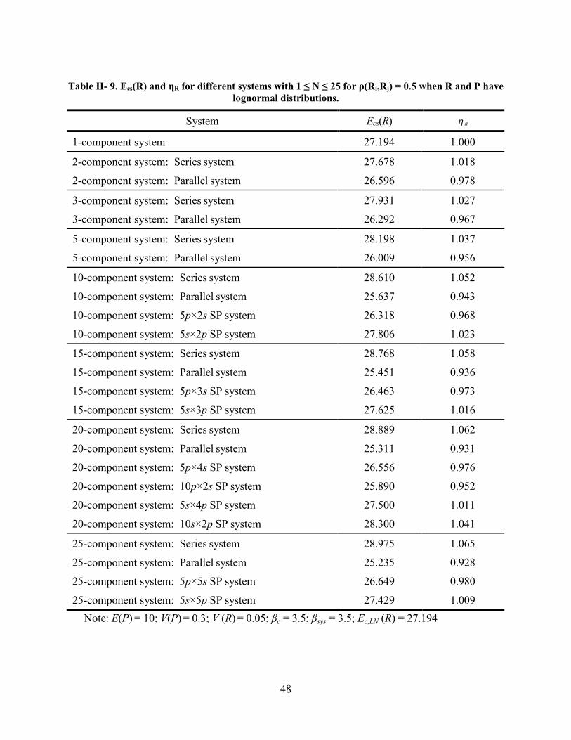
48
Table II- 9. Ecs(R) and ηR for different systems with 1 ≤ N ≤ 25 for ρ(Ri,Rj) = 0.5 when R and P have lognormal distributions.
System Ecs(R) h R
1-component system 27.194 1.000
2-component system: Series system 27.678 1.018
2-component system: Parallel system 26.596 0.978
3-component system: Series system 27.931 1.027
3-component system: Parallel system 26.292 0.967
5-component system: Series system 28.198 1.037
5-component system: Parallel system 26.009 0.956
10-component system: Series system 28.610 1.052
10-component system: Parallel system 25.637 0.943
10-component system: 5p×2s SP system 26.318 0.968
10-component system: 5s×2p SP system 27.806 1.023
15-component system: Series system 28.768 1.058
15-component system: Parallel system 25.451 0.936
15-component system: 5p×3s SP system 26.463 0.973
15-component system: 5s×3p SP system 27.625 1.016
20-component system: Series system 28.889 1.062
20-component system: Parallel system 25.311 0.931
20-component system: 5p×4s SP system 26.556 0.976
20-component system: 10p×2s SP system 25.890 0.952
20-component system: 5s×4p SP system 27.500 1.011
20-component system: 10s×2p SP system 28.300 1.041
25-component system: Series system 28.975 1.065
25-component system: Parallel system 25.235 0.928
25-component system: 5p×5s SP system 26.649 0.980
25-component system: 5s×5p SP system 27.429 1.009Note: E(P) = 10; V(P) = 0.3; V (R) = 0.05; βc = 3.5; βsys = 3.5; Ec,LN (R) = 27.194

49
Table II- 10. Ecs(R) and ηR for different systems with 50 ≤ N ≤ 100 for ρ(Ri,Rj) = 0.5 when R and P have lognormal distributions.
System Ecs(R) h R
50 component system: Series system 29.290 1.077
50 component system: Parallel system 24.969 0.918
50 component system: 5p×10s SP system 26.796 0.985
50 component system: 10p×5s SP system 26.187 0.963
50 component system: 5s×10p SP system 27.190 1.000
50 component system: 10s×5p SP system 27.865 1.025
100 component system: Series system 29.537 1.086
100 component system: Parallel system 24.748 0.910
100 component system: 5p×10s SP system 27.038 0.994
100 component system: 10p×10s SP system 26.344 0.969
100 component system: 20p×5s SP system 25.784 0.948
100 component system: 5s×20p SP system 27.000 0.993
100 component system: 10s×10p SP system 27.690 1.018
100 component system: 20s×5p SP system 28.247 1.039Note: E(P) = 10; V(P) = 0.3; V (R) = 0.05; βc = 3.5; βsys = 3.5; Ec,LN (R) = 27.194

50
Table II- 11. Ecs(R) and ηR for different systems with 1 ≤ N ≤ 25 for ρ(Ri,Rj) = 1.0 when R and P have lognormal distributions.
System Ecs(R) h R
1-component system: 27.194 1.000
2-component system: Series system 27.190 1.000
2-component system: Parallel system 27.190 1.000
3-component system: Series system 27.190 1.000
3-component system: Parallel system 27.190 1.000
5-component system: Series system 27.190 1.000
5-component system: Parallel system 27.190 1.000
10-component system: Series system 27.198 1.000
10-component system: Parallel system 27.198 1.000
10-component system: 5p×2s SP system 27.198 1.000
10-component system: 5s×2p SP system 27.198 1.000
15-component system: Series system 27.198 1.000
15-component system: Parallel system 27.198 1.000
15-component system: 5p×3s SP system 27.198 1.000
15-component system: 5s×3p SP system 27.198 1.000
20-component system: Series system 27.198 1.000
20-component system: Parallel system 27.198 1.000
20-component system: 5p×4s SP system 27.198 1.000
20-component system: 10p×2s SP system 27.198 1.000
20-component system: 5s×4p SP system 27.198 1.000
20-component system: 10s×2p SP system 27.198 1.000
25-component system: Series system 27.201 1.000
25-component system: Parallel system 27.201 1.000
25-component system: 5p×5s SP system 27.201 1.000
25-component system: 5s×5p SP system 27.201 1.000Note: E(P) = 10; V(P) = 0.3; V (R) = 0.05; βc = 3.5; βsys = 3.5; Ec,LN (R) = 27.194
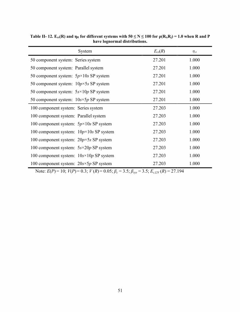
51
Table II- 12. Ecs(R) and ηR for different systems with 50 ≤ N ≤ 100 for ρ(Ri,Rj) = 1.0 when R and P have lognormal distributions.
System Ecs(R) h R
50 component system: Series system 27.201 1.000
50 component system: Parallel system 27.201 1.000
50 component system: 5p×10s SP system 27.201 1.000
50 component system: 10p×5s SP system 27.201 1.000
50 component system: 5s×10p SP system 27.201 1.000
50 component system: 10s×5p SP system 27.201 1.000
100 component system: Series system 27.203 1.000
100 component system: Parallel system 27.203 1.000
100 component system: 5p×10s SP system 27.203 1.000
100 component system: 10p×10s SP system 27.203 1.000
100 component system: 20p×5s SP system 27.203 1.000
100 component system: 5s×20p SP system 27.203 1.000
100 component system: 10s×10p SP system 27.203 1.000
100 component system: 20s×5p SP system 27.203 1.000Note: E(P) = 10; V(P) = 0.3; V (R) = 0.05; βc = 3.5; βsys = 3.5; Ec,LN (R) = 27.194