1. ANDERSON’S BRIDGE

OBJECTIVE:

To measure the value of unknown inductance with the help of Anderson’s bridge.

APPARATUS REQUIRED:

1. Anderson’s bridge trainer kit. 2. 2mm patch chords. 3. Digital multimeter.

CIRCUIT DIAGRAM:

PROCEDURE: 1. Make the connections as per the circuit diagram. 2. Connect the one pair of end terminals to the input supply.and other end terminals are

connected to the Differential amplifier. 3. Set the amplitude knob in maximum position. 4. Rotate the Potentiometer will equal to the r1= 123.8Ω. per unknown inductor Lx1. 5. Switch on the power supply. Now connect the head phone to audio socket. 6. Rotate the potentiometer r to find a condition where null or minimum sound is generated. 7. For different combinations of L and R, vary the r where null or minimum sound is

generated. 8. Switch off the power supply take the readings of variable resistance r and calculate the

unknown inductance.

TABULAR COLUMN: S.NO. r(Ω)measured r1(Ω)measured Rx(Ω)conducted Lx(μH)calculated 1 0.643 123.5 326.79 173.5 2 1.286 123.5 326.79 314.3 3 1.702 123.5 326.79 416.3

CALCULATIONS: Calculated value of Lx =CR3/R4(r(R4+R2)+R4.R2) Calculates the value of Rx =R2.R3/R4-r1 RESULT:

The value of unknown inductance is calculated by using Anderson’s bridge trainer kit.

2. DE SAUTY’S BRIDGE

Technical Specifications

SINE WAVE GENERATOR

Frequency : 1kHZ ± 10%

Amplitude : Upto 15 Vpp

Fuse : 15mA

Mains Supply : 230 V ±10%,50Hz

Unknown Capacitors : 0.1µF,0.22µF,0.47µF

OBJECTIVE:

Determination of unknown capacitance using De Sauty’s Bridge method.

ITEMS REQUIRED:

1. De Sauty’s Bridge Trainer

2. 2mm Patch cords

3. Multimeter

CIRCUIT DIAGRAM:

PROCEDURE:

1. Make the connections as per the circuit diagram. 2. Connect the one pair of bridge end terminals to the null detector section 3. and the input terminls are connected to output terminals 4. Set the R1 knob in minimum position. 5. Set the amplitude knob in maximum position. 6. Switch on the power supply.. 7. For different combinations of unknown capacitance ,vary the R1 knob until the null

detection section shows zero reading and at that instant note down the value of R1. 8. Now calculate the values of Cx1,Cx2 and Cx3 in each case. 9. Switch off the power supply to the trainer kit.

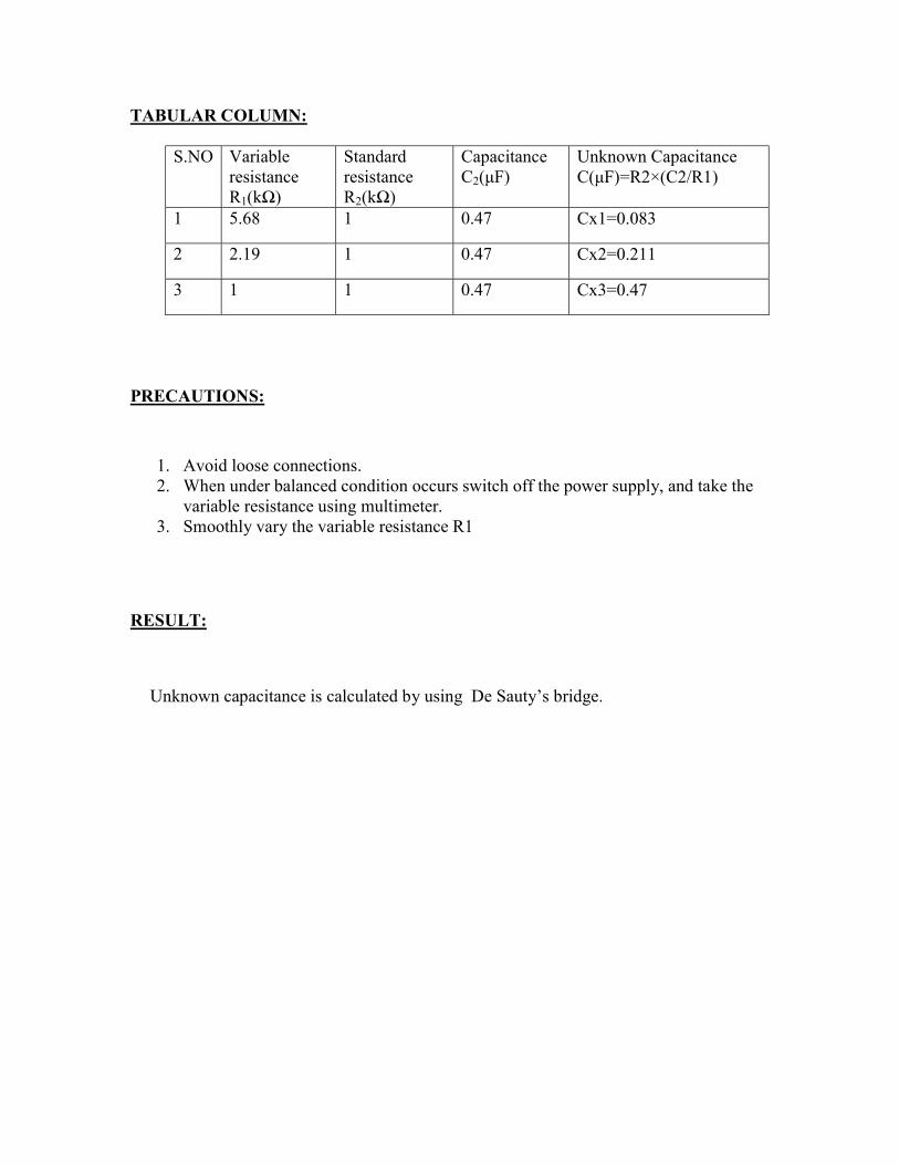
TABULAR COLUMN:

S.NO Variable resistance R1(kΩ)

Standard resistance R2(kΩ)

Capacitance C2(μF)

Unknown Capacitance C(μF)=R2×(C2/R1)

1 5.68 1 0.47 Cx1=0.083

2 2.19 1 0.47 Cx2=0.211

3 1 1 0.47 Cx3=0.47

PRECAUTIONS:

1. Avoid loose connections. 2. When under balanced condition occurs switch off the power supply, and take the

variable resistance using multimeter. 3. Smoothly vary the variable resistance R1

RESULT:

Unknown capacitance is calculated by using De Sauty’s bridge.

3. SCHERING BRIDGE

OBJECTI VE:

Determination of unknown capacitance using Schering Bridge method.

ITEMS REQUIRED:

1. Schering Bridge Trainer

2. 2mm Patch cords

3. Multimeter

CIRCUIT DIAGRAM:

PROCEDURE:

1) Make the connections as per the circuit diagram. 2) Connect the one pair of bridge end terminals to the null detector section. 3) And the other input terminals are connected to output terminals of the bridge. 4) Set the R1 knob in minimum position. 5) Set the amplitude knob in maximum position.

6) Switch on the power supply.. 7) For different combinations of unknown capacitance ,vary the R1 knob until the null

detection section shows zero reading and at that instant note down the value of R1. 8) Now calculate the values of Cx1,Cx2 and Cx3 in each case. 9) Switch off the power supply to the trainer kit.

TABULAR COLUMN:

S.NO Variable

resistance R1(kΩ)

Standard resistance R2(Ω)

Capacitance C2(μF)

Unknown Capacitance C(μF)=R2×(C2/R1)

1 2.57 470 0.47 Cx1=0.085

2 1.11 470 0.47 Cx2=0.199

3 0.55 470 0.47 Cx3=0.409

PRECAUTIONS:

1) Avoid loose connections.

2) When under balanced condition occurs switch off the power supply, and take the variable resistance using multimeter.

RESULLT:

Unknown capacitance is calculated by using Schering bridge.

4. HAY’S BRIDGE

Sine Wave Generator

Frequency : 1kHZ to 10kHZ ±10%

Amplitude : 0 to 5 Vpp

DPM : 0-200mV

Unknown Inductors: 58mH ± 10% with 58 Ω ± 10% of resistance

100mH ± 5% with 174 Ω ± 5% of resistance

116mH ± 10% with 116 Ω ± 10% of resistance

Mains Supply : 230V ± 10%, 50Hz

OBJECTIVE:

Determination of unknown inductance and Q factor using Hay’s bridge method

Apparatus:

1. Scientech 5356 trainer 2. 2mm patch cords 3. CRO 4. Digital multimeter

CIRCUIT DIAGRAM:

PROCEDURE:

1. Make the connections as per the 2. Set the frequency of the sine wave generator to 2kHz by connecting its terminals to

CRO. 3. Set the amplitude of sine wave using

wave generator section as per your convenience.

4. Connect one end pair of the brito the bridge.

5. Connect the other end pair terminals to the null detector section.6. Connect the combination of C1 and R11 to the and Lx1 and Rx1 into the circuit.7. For known value of R3, vary the R2

reading. 8. At this instant calculate the value of Lx1 and Rx1.9. Repeat the above procedure for different combinations of C and R1.10. Switch off the power supply.

Make the connections as per the circuit diagram. Set the frequency of the sine wave generator to 2kHz by connecting its terminals to

Set the amplitude of sine wave using Amplitude Control knob in sine

wave generator section as per your convenience.

Connect one end pair of the bridge terminals to the sinewave generator section as input

Connect the other end pair terminals to the null detector section. Connect the combination of C1 and R11 to the and Lx1 and Rx1 into the circuit.For known value of R3, vary the R2 knob untill the null detector shows the zero

At this instant calculate the value of Lx1 and Rx1. Repeat the above procedure for different combinations of C and R1. Switch off the power supply.

Set the frequency of the sine wave generator to 2kHz by connecting its terminals to

knob in sine

dge terminals to the sinewave generator section as input

Connect the combination of C1 and R11 to the and Lx1 and Rx1 into the circuit. knob untill the null detector shows the zero

TABULAR COLUMN:

C1 and R11

R3(Ω) R-

1x(Ω) Cx(nF) R2(kΩ) Lx(mH) Rx(Ω) Q1

500 28 220 0.552 60.36 58.65 12.93 500 28 220 0.738 80.69 78.42 12.97 500 28 220 0.910 99.5 96.69 12.93

C2 and R12

500 20 330 0.435 71.29 74.22 12.06 500 20 330 0.775 127 132.25 12.063 500 20 330 0.911 149.29 155.44 12.063

C3 and R13

500 13 470 0.351 82 79.04 13.03 500 13 470 0.605 140.6 185.56 13.03 500 13 470 0707 165.2 159.21 13.03

FORMULAS USED:

𝐿1 =𝑅2 × 𝑅3 × 𝐶4

(1 + 𝜔 × 𝑅4 × 𝐶4 )

𝑅1 =𝜔 × 𝑅2 × 𝑅3 × 𝑅4 × 𝐶4

(1 + 𝜔 × 𝑅4 × 𝐶4 )

𝑄 =𝜔 × 𝐿1

𝑅1=

1

𝜔 × 𝑅4 × 𝐶4

RESULT: The values of unknown Inductance and Q-factor are determined using Hay’s Bridge trainer kit.

5. KELVIN’S BRIDGE

Technical specifications

Mains supply : 230V ±10%,50HZ

DC Power supply : +5V

Unknown Resistors : 0.3Ω,0.4Ω,0.8Ω

Known Resistors : R1=100KΩ,20KΩ,10KΩ

R3=1KΩ,200Ω,100Ω

DPM : 2V

OBJECTIVE:

Determination of low resistance using Kelvin’s Bridge method.

ITEMS REQUIRED:

1. Kelvin’s Bridge trainer kit 2. Digital Multi meter 3. 2 mm patch chords

CIRCUIT DIAGRAM:

PROCEDURE:

1) Make the connections as per the circuit diagram. 2) Connect the galvanometer end terminals to the null detector section. 3) Set the R2 knob in minimum position.

4) Adjust the ratio of r1 and r3 such that it is equal to the ratio of R1 and R3.i.e 100:1 5) Connect r1 and r3 with a 2mm patch card. 6) For different combinations of R1 and R3 vary the R2 knob until the null detection section

shows zero reading switch off the power supply and at that instant note down the value of R2.

7) Now calculate the values of Rx1,Rx2 and Rx3 in each case. 8) Switch off the power supply to the trainer kit.

TABULAR COLUMN:

Rx1

R1(kΩ) R3(kΩ) R2(kΩ) Rx(kΩ)=(R2×R3)/R1 100 1 96 0.96 20 0.2 95.4 0.95 10 0.1 90 0.9

Rx2 100 1 51 0.51 20 0.2 50 0.5 10 0.1 49.9 0.49

Rx3 100 1 36.5 0.36 20 0.2 36 0.36 10 0.1 35.5 0.35

RESULT: unknown resistance is determined by using kelvins bridge

6. MAXWELL’S BRIDGE

Technical Specifications

Mains supply : 230V AC ± 10%,50Hz

DC power supply : ± 12V

Sine wave generator

Fixed frequency : 1 kHZ ± 5%

Amplitude control range : Up to 20Vpp

DPM : 200mV

Unknown Inductors : 56 µH ,24 µH,12µH,10mH,20mH,30mH

OBJECTIVE:

Determination of unknown inductance using Maxwell‟s inductance bridge method.

ITEMS REQUIRED:

1) Maxwell’s trainer kit

2) 2 mm patch cords 3) Digital Multimeter 4) Oscilloscope

CIRCUIT DIAGRAM:

PROCEDURE:

1) Make the connections as per the circuit diagram. 2) Connect the one pair of bridge end terminals to the null detector section. 3) And other input terminals are connected to output terminals. 4) Set the R2 knob in minimum position. 5) Set the amplitude in maximum position. i.e., 1 kHz. 6) For different combinations of R and L vary the R2 knob until the null detection section

shows zero reading . 7) Switch off the power supply, note the values of R2 by using multimeter. 8) Now calculate the values of unknown resistance(Rx)and inductance(Lx), in each case. 9) Switch off the power supply to the trainer kit.

TABULAR COLUMN:

Cases R2(Ω) R4(Ω) R3(Ω) L1(μH) Lx=R2.L1/R4(μH) Rx=R2.R3/R4(Ω) 1 270 100 120.8 12.1 32.67 326.16 2 198 100 237.9 12.1 23.9 471 3 110.9 100 470 12.1 13.4 521.2

RESULT:

The unknown resistance and inductance values are calculated by using Maxwell’s inductance bridge.

7. MAXWELL’S INDUCTANCE CAPACITANCE BRIDGE

OBJECTIVE:

Determination of unknown inductance and Q-factor using Maxwell‟s inductance capacitance bridge method

ITEMS REQUIRED:

1. Maxwell’s bridge trainer kit.

2. 2mm patch cords

3. Digital Multimeter

4. Oscilloscope

CIRCUIT DIAGRAM:

PROCEDURE:

1) Make the connections as per the circuit diagram. 2) Connect the one pair of bridge end terminals to the null detector section. 3) And other input terminals are connected to output terminals. 4) Set the R4 knob in minimum position. 5) Set the amplitude in maximum position.i.e., 1 kHz. 6) For different combinations of R and L vary the R4 knob until the null detection section

shows zero reading and at that instant note down the value of R4. 7) Switch off the power supply,note the values of R4 by using multimeter. 8) Now calculate the values of unknown resistance(Rx)and inductance(Lx) and Q factor, in

each case. 9) Switch off the power supply to the trainer kit. TABULAR COLUMN:

S.NO.

R2(Ω)

Variable resistanceR4(Ω)

R3(kΩ)

C1(nF)

Unknown inductanceLx=R4.R2.C1(mH)

Unknown resistanceRx=R2.R4/R3(Ω)

Q=ⱷLx/Rx=ⱷC1.R3

1 221 118 1.122 330 8 23 2.18

2 221 236 1.122 330 17 46 2.32

3 221 319 1.122 330 23 62 2.32

RESULT: The unknown values of resistance, inductance and also Q- factor is calculated by using Maxwell’s inductance capacitance bridge.

9. SLIDE WIRE POTENTIOMETER

OBJECTIVE:

Calibration of voltmeter and ammeter by using slidewire potentiometer

ITEMS REQUIRED

1) Potentiometer 2) Sliding jockey 3) Mains cord 4) Patch cords

CIRCUIT DIAGRAM:

PROCEDURE:

CALIBRATION OF VOLTMETER:

1. Initially test the supply voltage to the potentiometer trainer kit by connecting one of the terminals of the digital voltmeter to the DC supply and the other terminal to the ground of the DC potentiometer.

2. By connecting the digital ammeter terminals to the DC potentiometer and connect dc potentiometer terminals to the X and Z terminals.

3. Connect the galvanometer positive terminal to the jockey and negative terminal to the dc supply adjust the ammeter reading to 30mA by varying the VR2 knob.

4. Touch the jockey to X and Z terminals observe the reading in galvanometer 5. Now slide the jockey on potentiometer wire and find null point Now measure the

distance L moved from Z terminal to null point L=[(n-1)*100+r] 6. Divide output of dc supply Vdc to the distance L. this will give a constant C which is

voltage drop per cm C=Vdc /L 7. Now disconnect DC supply from galvanometer negative terminal. 8. Connect the variable voltage VR1 to the input supply in the voltmeter section. 9. Connect the input and output terminals of the voltage divider in voltmeter section to

the voltage divider circuit 10. Connect an analog voltmeter to the voltage in the voltmeter section. 11. Connect negative terminal of galvanometer to the ending terminal of the voltage divider

in the voltmeter section. 12. Vary the VR1 knob to adjust the voltmeter reading to 1V. 13. Now slide the jockey on the DC potentiometer until the galvanometer reads zero. 14. Note down the length of the wire corresponding to the zero reading. 15. Repeat the above procedure for different values of standard voltages.

TABULAR COLUMN: CALIBRATION OF VOLTMETER:

S.No

DC Voltmeter Reading(V)

Null point position D(cm)

Voltage Ratio(M)

Voltage across potentiometer Vp=C×D×M

% Error= × 100

1 1 894 1 1.1 -15 2 2 274 10 3.6 -44 3 3 363 10 4.7 -36 4 4 456 10 6.01 -33 5 5 545 10 7.19 -30 6 6 624 10 8.23 -27 7 7 712 10 9.3 -24 8 8 805 10 10.6 -24 9 9 484 10 12.7 -29

CALIBRATION OF AMMETER: 1. Initially test the supply voltage to the potentiometer trainer kit by connecting one of the

terminals of the digital voltmeter to the DC supply and the other terminal to the ground of the DC potentiometer.

2. By connecting the digital ammeter terminals to the DC potentiometer and connect dc potentiometer terminals to the X and Z terminals.

3. Connect the galvanometer positive terminal to the jockey and negative terminal to the dc supply adjust the ammeter reading to 35mA by varying the VR2 knob.

4. Touch the jockey to X and Z terminals observe the reading in galvanometer 5. Now slide the jockey on potentiometer wire and find null point Now measure the

distance L moved from Z terminal to null point L=[(n-1)*100+r] 6. Divide output of dc supply Vdc to the distance L. this will give a constant C which is

voltage drop per cm C=Vdc /L 7. Now disconnect DC supply from galvanometer negative terminal

8. Connect the variable voltage VR1 to the input supply in the ammeter section.

9. Connect the input and output terminals of the voltage divider in ammeter section to

the voltage divider circuit

10. Connect the variable resistance in series with the input terminals of the ammeter

section and also connect an analog ammeter to the ammeter in ammeter section.

11. Connect the negative terminal of galvanometer to the end terminal of the voltage divider in ammeter section

12. Vary the VR2 knob to adjust the ammeter reading to 0.1A.Now slide the jockey on the DC potentiometer until the galvanometer reads zero.

13.Note down the length of the wire corresponding to the zero reading.

14.Repeat the above procedure for different values of standard currents.

15.Switch off the power supply.

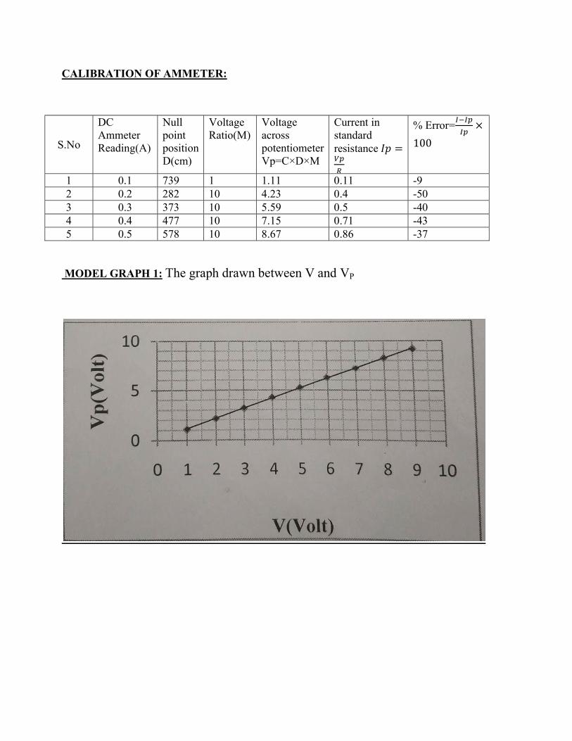
CALIBRATION OF AMMETER:

S.No

DC Ammeter Reading(A)

Null point position D(cm)

Voltage Ratio(M)

Voltage across potentiometer Vp=C×D×M

Current in standard resistance 𝐼𝑝 =

% Error= ×

100

1 0.1 739 1 1.11 0.11 -9 2 0.2 282 10 4.23 0.4 -50 3 0.3 373 10 5.59 0.5 -40 4 0.4 477 10 7.15 0.71 -43 5 0.5 578 10 8.67 0.86 -37

MODEL GRAPH 1: The graph drawn between V and VP

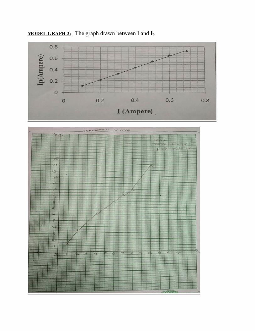
MODEL GRAPH 2: The graph drawn between I and IP

RESULT: given voltmeter and ammeter is calibrated and also error will be calculated by using slide wire potentiometer

9. DC CROMPTON’S POTENTIOMETER

OBJECTIVE:

To calibrate PMMC Voltmeter and Ammeter by DC Crompton’s potentiometer

APPARATUS:

S. No. Equipment Range Quantity

1 DC Crompton’s potentiometer Kit 1.5V/250mV 1

2 Standard Cell 1.0180V 1

3 2 Channel RPS 30V/2A 1

4 Voltmeter 0-300V 1

5 Ammeter 0-5A 1

6 Standard Resistance Box/DRB 0.1Ω 1

7 Voltage Ratio Box 0-300V

8 Galvanometer 1

9 Patch Chords required

CIRCUIT DIAGRAM:

Fig – 3.1 Standardization

Fig

3.1 Standardization

Fig – 3.2 Calibration of Voltmeter

PROCEDURE:

Calibration Of Ammeter:

1. Connections are given as per the block diagram.

2. Switch on the 2V D.C . power supply to the potentiometer kit.

3. Adjust the potentiometer voltage dial to 1.0186V and switch on the supply.

4. Observe the deflection in the galvanometer by pressing the standardization knob on the meter kit.

5. If deflection is not zero, then adjust the fine and coarse knobs until there is no deflection in the galvanometer.

6. Now the potentiometer is standardized.

Calibration of Voltmeter:

1. Connections are given as per the block diagram.

2. Apply test voltage. Reset the potentiometer dial reading closer to the applied test voltage.

3. Now by pressing the test button observe the deflection in the galvanometer.

4. Vary the dial reading until there is no deflection in the galvanometer.

5. Now note down the readings of Voltmeter, Potentiometer dial and calculate the error.

6. Repeat this procedure for different test voltages and find the error in the voltmeter.

Calibration of ammeter:

1. Connections are given as per the block diagram 2. Apply test voltage up to 30V. Reset the potentiometer dial reading closer to the applied test

voltage.

3. Now by pressing the test button observe the deflection in the galvanometer.

4. Vary the dial reading until there is no deflection in the galvanometer.

5. Now note down the readings of Ammeter, Potentiometer dial, Resistance and calculate the error.

6. Repeat this procedure for different values of Resistance and find the error in the Ammeter.

Tabular column:

Voltmeter calibration:

S. No Voltage Potentiometer % Error

Reading(Vm) Reading(VP)

1 30(1.5) 1.47 1.6

2 15(1.5) 1.47 1.5

3 1.5(1.5) 1.571 -4.5

Ammeter calibration:

S. No Resistance Current in the Potentiometer Current in the % Error

(R)ohm circuit (Ic)mA Reading (VP)V circuit (Ic)mA

1

2

3

MODEL CALCULATIONS:

Voltmeter Calibration

% Error in Meter = [(Vm–Vp)*100]/Vm

Ammeter Calibration

Current in the circuit Ic = [VP/R]

% Error in Meter = [(Im–Ic)*100]/Im

10. CALIBRATION OF POWER FACTOR METER

Objective:

To calibrate dynamometer type power factor meter.

APPARATUS

S. No Equipment Range Type Quantity 1 Power factor meter 600V/5A 1 2 Voltmeter (0-300V) Digital 1 3 Ammeter (0-5A) Digital 1 4 Loads R,L,C 4A each 5 Wattmeter 250V/5A UPF 1 6 1φ variac (0-270V)/10A 1 7 Connecting Wires As Required

CIRCUIT DIAGRAM:

Calibration of Dynamo Meter Type Power Factor Meter

PROCEDURE:

Make the connections as per the circuit diagram.

Keep the Autotransformer at zero position.

Switch on the 230 VAC, 50 Hz, power supply.

Increase the input voltage gradually by rotating the Autotransformer in clockwise direction.

w, by switching on different loads note down the corresponding values of voltmeter, ammeter,

wattmeter and power factor meter for different values of individual loads and also their

combinations.

Switch off all the loads and bring back the auto transformer to its initial position.

Switch off the power supply.

TABULAR COLUMN:

S.No Applied Load(A)

Voltmeter Reading (V)

Ammeter Reading(A)

Wattmeter(W) PF meter Reading(X)

PF calculated(Y)

Cos φ=W/VI

% Error

× 100

1 R-Load-1

228.1 2.10 515 1 1.0725 7.25

2 R-Load-2

226.3 4.12 980 1 1.049 4.91

3 L-Load-1

229 2.27 20 - 0.0382lag -

4 L-Load-2

229 4.65 80 - 0.0748lag -

5 C-Load-1

230 1.55 00 - 0 -

6 C-Load-2

230 3.10 00 - 0 -

7 RL-Load-1

229 1.28 220 0.66lag 0.7459lag 13.015

8 RL-Load-2

228 2.61 440 0.69lag 0.736lag 6.66

9 RC-Load-1

230 1.25 190 0.73lead 0.65lead -9.72

10 RC-Load-2

228 2.47 370 0.62lead 0.654lead 5.48

11 RLC-Load-1

229 1.88 450 0.98lead 1.039lead 6.02

12 RLC-Load-2

227 3.74 390 0.96lead 1.0289lead 7.17

RESULT: % Error of the given power factor meter is calibrated at different loads.

11.CALIBRATION OF LPF-WATTMETER BY PHANTOM LOADING

Objective:

To calibrate a given LPF Wattmeter by phantom testing method.

Apparatus Required:

S.No Equipment Range Type Quantity 1 LPF Wattmeter (150/300/600V)/5A Dynamometer 1 2 Voltmeter (0-300V) Digital 1 3 Ammeter (0-5A) Digital 1 4 Inductive load (0-150mH)/5A 1 5 1φ variac (0-270V)/10A 1 6 Connecting Wires As Required

Theory:

Measurement of power in circuits having low power factor by ordinary electro dynamometer watt meters is difficult and inaccurate because

1) The deflecting torque on the moving systems is small even when the

current and pressure coils and fully excited.

2) Errors introduced because of inductance of pressure coil tend to be large

at low power factors, special features are incorporated in an electro

dynamometer wattmeter to make it a low power factor type of

wattmeter. These features are discussed in detail below.

Compensation for pressure coil current. Compensation for Inductance of pressure coil. (c ) Small control torque. (d) Pressure coil current

Circuit Diagram:

Procedure:

1) Connections are made as per circuit diagram. 2) Kept the Auto Transformers ( 1 & 2 ) in minimum position. 3) Adjust the voltage of the autotransformer which is connected to the pressure coil of the

wattmeter to 230V. 4) Now by varying the autotransformer which is connected to the load in steps of 0.5A, note

down the values of voltmeter, ammeter and wattmeter. 5) The experiment is repeated for different values of current at constant voltage. 6) After noting the values slowly decrease the auto transformers till Ammeter and Voltmeter

comes to zero position and switch off the supply.

TABULAR COLUMN:

S. No

Applied Load(A)

Voltmeter Reading(V)

Wattmeter(X) True Power Y=VIcosφ

% Error=(X-Y)/Y×100

1 0.5 220 60 89.88 -33

2 1 219.3 130 176 -26

3 1.5 218.2 210 263.1 -20

4 2 216.8 296 349.12 -15

5 2.5 216.5 376 433.6 -13

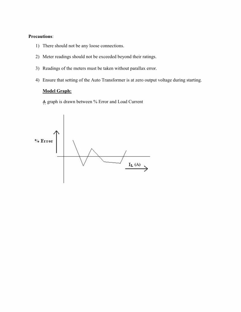
Precautions:

1) There should not be any loose connections.

2) Meter readings should not be exceeded beyond their ratings.

3) Readings of the meters must be taken without parallax error.

4) Ensure that setting of the Auto Transformer is at zero output voltage during starting. Model Graph: A graph is drawn between % Error and Load Current 7.

Result:

Calibration of given LPF Wattmeter is done by Phantom testing and the error is calculated.

12. CALIBRATION OF 1-PHASE ENERGY METER Objective: To calibrate and testing of single phase induction type energy meter.

APPARATUS

S. No Equipment Range Type Quantity 1 Energy meter 3200 rev/kwhr Induction 1 2 Voltmeter (0-300V) Digital 1 3 Ammeter (0-10A) Digital 1 4 Resistive load 1 5 Stop Watch 1 6 1φ variac (0-270V)/10A 1 7 Connecting Wires As Required

CIRCUIT DIAGRAM:

Fig – 1.1 Calibration and Testing of Single Phase Energy Meter

PROCEDURE:

Make the connections as per the circuit diagram.

Keep the Autotransformer at zero position.

Switch on the 230 VAC, 50 Hz, power supply.

Increase the input voltage gradually by rotating the Autotransformer in clockwise

direction.

Adjust the resistive load so that sufficient current flows in the circuit. Please note that the

current should be less than 5A.

Note down the Voltmeter and ammeter readings for different loads as per the tabular

column.

Note down the time (by using stop watch) for rotating the disc of the Energy Meter for 10

times at each load.

Bring back the auto transformer to its initial position and switch off the power supply.

TABULAR COLUMN:

S.No

Applied Load(A)

Voltmeter Reading (V)

Ammeter Reading(A)

R=Number of revolutions of disc

Time(sec)

ES(kwhr) ET(kwhr) % Error

1 1 229.6 1.04 10 41 3.125x10-3

2.734x10-3

14.9

2 2 227.6 2.22 10 19 3.125x10-3

2.614 x10-3

17.2

3 3 226.7 3.24 10 13 3.125x10-3

2.85 x10-

3 17.42

4 4 224.9 4.24 10 11 3.125x10-3

2.95 x10-

3 7.02

5 5 224.3 5.24 10 9 3.125x10-3

2.911 x10-3

5.89

MODEL CALCULATIONS:

Energy meter constant K is defined as

Energy recorded by meter under test = Rx / Kx – kWh.

Energy computed from the readings of the indication instrument = kW x t

Where

Rx = number of revolutions made by disc of meter under test.

Kx = number of revolutions per k Wh for meter under test.

KW = Power in kilowatt as computed from readings watt meter indicating instruments

t = time in hours.

For 1A load:

𝐸 =228 × 1.04 × 10 × 40

3600 × 1000

= 2.634 × 10 𝑘𝑊ℎ

%𝐸𝑟𝑟𝑜𝑟 =3.125 × 10 − 2.634 × 10

2.634 × 10× 100

= 18.64%

Precautions:

1) There should not be any loose connections.

2) Meter readings should not be exceeded beyond their ratings.

3) Readings of the meters must be taken without parallax error.

4) Ensure that setting of the Auto Transformer is at zero output voltage during starting.

Model Graph: A graph is drawn between % Error and Load Current

RESULT:

Calibration of 1φ energy meter has been done and error is calculated.

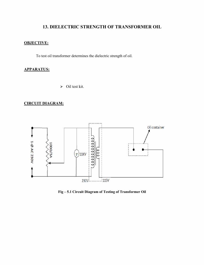
13. DIELECTRIC STRENGTH OF TRANSFORMER OIL

OBJECTIVE:

To test oil transformer determines the dielectric strength of oil.

APPARATUS:

Oil test kit.

CIRCUIT DIAGRAM:

Fig – 5.1 Circuit Diagram of Testing of Transformer Oil

PROCEDURE:

1) The oil is poured in a container known as test cell the electrodes are polish spheres perfectly of brass arranged horizontally a suitable gauge is used to adjust the gap.

2) While pouring the oil sample the test cell(container should )be thoroughly cleaned & the

moisture & spended particles should be avoided in fig shown below & experimental setup for finding out the dielectric strength of the give sample of oil.

3) The voltmeter is the connected on the primary side of high voltage side transformer for calibration.

4) Adjust the gap between the spheres is to 4MM with the help of gauge then pour transformer oil till a depth slurries are immersed.

5) Then increase the voltage gradually & continuously till a flashover of the gap is seen on the MCB apparatus note down this voltage. This voltage is known as rapidly applied voltage.

6) The breakdown of the gap has taken please mainly due to field effect. The thermal effect is main as the time of application is short.

7) Next bring the voltage back Zero & star with 40% of rapidly applied voltage & weight for one min.sec if the flashover by take occurred if not increase the voltage every time by of the rapidly applied voltage and wait for one min till the flash over is seen on the MCB trips. Note the voltage.Repeat the experiment with different values of voltage.

8) The acceptable value is 30KV for 4mm & 2.5mm for 11KV the oil should be set for secondly.

TABULR COLUMN:

S.NO. Dielectric strength of oil in kV

1 57.3 2 44.7 3 61.6 4 44.5 5 55.1 6 50.6 7 46.5

Average= . . . . . . .

𝟕 = 51.48kV

PRECAUTIONS:

It is to be noted that the electrodes are immersed vertically in the oil. It is due to the fact that when oil decomposes. Carbon particles being lighter rice up & if electrons are vertical configurations, this well bridge the gap & the breakdown will take place.

RESULT:

Dielectric strength of transformer oil has been calculated.

14. CT TESTING BY COMPARISON METHOD

AIM:

To obtain the ratio and phase angle errors of the given current transformer (C.T).

APPARATUS REQUIRED:

S.No Equipment Range Type Quantity 1 Wattmeters 250V/5A UPF 2 2 Burden 75Ω Resistive 1 3 Ammeter (0-10/20A) Digital 2 4 Phase shifting

Transformer 500VA Deflecting 1

5 Current Transformers(standard and under Test)

20/5A,10/5A Instrument 1

6 1φ variac (0-270V)/20A 1 7 Connecting Wires As Required

Theory:

Silsbee’s method is a comparison method. There are two types of Silsbee’s methods: deflection and null. Only deflection method is described here. Here the ratio and phase angle of the test transformer X are determined, in terms of that of a standard transformer S having the same nominal ratio. The two transformers are connected with their primaries in series. An adjustable burden is put in the secondary circuit of the transformer under test. An ammeter is included in the secondary circuit of the standard transformer so that the current may be sent to the desired value.W1 is a wattmeter whose current coil is connected to carry the secondary current of the standard transformer. The current coil of wattmeter W2 carries current ΔI which is the difference between the secondary currents of the standard and test transformer S, X.

The voltage circuits of the wattmeter’s (i.e. their pressure coils) are supplied in parallel from a phase shifting transformer at a constant voltage V. This is a comparison type of test employing deflection methods. Here the ratio and phase angle of the test transformer X are determined in terms of that of a standard transformer S having the same nominal ratio.The errors are as follows say

CT Ratio error

S Rs

T RT

CIRCUIT DIAGRAM:

FORMULAE USED:

Nominal ratio (NR) of standard C.T = 2 (since 10/5 CT), (4 for 20/5 CT) The ratio of the C.T. under test RT is given by Actual ratio of standard C.T =NR(1+ R %Error = NR-AR/AR Phase angle error for the C.T Under test = Phase angle error of standard C.T Φ

Phase angle error

θs

θT

Nominal ratio (NR) of standard C.T = 2 (since 10/5 CT), (4 for 20/5 CT)

The ratio of the C.T. under test RT is given by𝑅 = 𝑅 (1 + )

Actual ratio of standard C.T =NR(1+ RT); 2(1+0.00882)=2.0176

Phase angle error for the C.T Under test = ѲT = + ѲS rad.

Phase angle error of standard C.T Φs = 8radians

PROCEDURE:

1) Make the connections as per the circuit diagram. 2) Adjust the phase of the primary current(I) of the standard transformer to rated value by

using the variac. 3) The phase of this current is to be adjusted with the help of phase shifting trnsformer

such that wattmeter W1 reads zero. Voltage V is in quadrature with current Iss as given in the phasor diagram (Fig 2).

4) Note the reading of the wattmeter W2. Let this be W2q. 5) The phase of the voltage V is shifted through 900 so that V is phase with Iss. Note the

readings of both Wattmeter’s W1 and W2. 6) Adjust the phase shifting transformer to zero degrees and at that instant note down the

values of both the wattmeters as W1P and W2P. 7) Bring back the autotransformer to its initial position and switch off the supply.

TABULAR COLUMN: S. No IP ISS W2q W1p W2p %Ratio

Error of test CT

Phase angle Error of test CT

% Ratio Error of standard CT

Phase angle Error of standard CT

1 10 4.95 290 1000 890 0.936 114.98 0.5 98.40

CALCULATIONS:

Nominal Ratio of standard CT=2(since 10/5A CT,4 for 20/5A CT)

Ratio Error of standard CT Rs=0.5%

Phase angle Error of standard CT θS=8 radians=8x(180/π)=458.40-3600=98.40

Phase angle Error of test CT=θT= (W2q/ W1p)+ θS =(290/1000)+8×(180/π)=114.980

%Error=(NR-AR)/AR×100 Nominal Ratio (NR)=Primary current/Secondary current=10/5=2 Actual ratio of standard CT=NR×(1+RT) RT =RS (1+W2P/W1P) =0.005(1+890/1000)=0.00945

AR=2×(1+0.00945)=2.0189 Ratio error of standard CT RS =0.5%

PHASOR DIAGRAM:

RESULT:

The ratio and phase angle errors of the given current transformer are determined.

15. PT –TESTING BY COMPARISION METHOD

OBJECTIVE:

To obtain the ratio and phase angle errors of the given potential transformer (P.T)

APPARATUS REQUIRED:

S.No Equipment Range Type Quantity 1 Wattmeters 250V/5A UPF 2 2 Voltmeter 0-400V Digital 2 3 Ammeter (0-5A) Digital 1 4 Phase shifting

Transformer 500VA Deflecting 1

5 Potential Transformers(standard and under Test)

400V/100V,200/100 V

Instrument 1

6 1φ variac (0-270V)/20A 1 7 Connecting Wires As Required

THEORY:

Method using Wattmeter’s this method is analogous to Silsbee’s deflection comparison method for potential transformers. The arrangement is shown in Fig 1. The ratio and phase angle errors of a test transformer are determined in terms of those of a standard transformer S having the same nominal ratio. The two transformers are connected with their primaries in parallel. A burden is put in the secondary circuit of test transformer.

W1 is a wattmeter whose potential coil is connected across the secondary of standard transformer. The pressure coil of wattmeter W2 is so connected that a voltage ΔV which is the difference between secondary voltages of standard and test transformers, is impressed across it. The current coils of the two watt meters are connected in series and are supplied from a phase shifting transformer. They carry a constant current I.

The errors are as follows

PT Ratio error Phase angle error

S Rs θs

T RT θT

FORMULAE USED:

%Error = NR-AR/AR×100

Ratio error of standard P.T, RS = 0.92%

Nominal ratio of standard P.T = 4(if 400V/100V=4,200V/100V=2)

Actual ratio of standard P.T =NR(1 + RT) ; 4 (1+0.0295)

The ratio of the P.T. under test RT i s given by RT = RS (1+W2p/W1p)

Phase angle error for the P.T Under t est = ѲT =(W2q/W1p) + ѲS rad.

Phase angle error of standard P.T ѲS = 3 rad.

CIRCUIT DIAGRAM:

PROCEDURE:

1) Make the connections as per the circuit diagram. 2) Adjust the phase of the primary voltage(v) of the standard transformer to rated value by

using the variac. 3) The phase of this voltage is to be adjusted with the help of phase shifting trnsformer

such that wattmeter W1 reads zero. Currnt I is in quadrature with current Vss as given in the phasor diagram (Fig 2).

Note the reading of the wattmeter W2. Let this be W2q. 4) The phase of the current I is shifted through 900 so that Ip is phase with Vss. Note the

readings of both Wattmeter’s W1 and W2. 5) Adjust the phase shifting transformer to zero degrees and at that instant note down the

values of both the wattmeters as W1P and W2P.

6) Bring back the autotransformer to its initial position and switch off the supply.

TABLAR COLUMN:

S. No VP(V) VSS(V) W2q W1p W2p %Ratio Error of test PT

Phase angle Error of test PT

% Ratio Error of standard PT

Phase angle Error of standard PT

1 391.5 97.9 4 41 99 -0.75% 177.180 0.92% 1710 or 3rad

CALCULATIONS:

Phase angle error of the test PT=θT=(W2q/ W1p)+ θS =(4/41)+3×(180/π)=177.180

% Ratio Error=(NR-AR)/AR×100 Nominal Ratio (NR)=Primary voltage/Secondary voltage=391.5/97.9=3.99

Actual Ratio of the test PT=NR×(1+RT);

=4×(1+3.13)

=16.12

Where, RT=RS(1+W2P/W1P) RT=0.92(1+99/41)=3.13 % ratio error= (4-16.12)/16.12= -0.75%

PHASOR DIAGRAM: RESULT:

The ratio and phase angle errors of the given potential transformer are determined.