arX

iv:c

ond-

mat

/991

0351

v1 [

cond

-mat

.sta

t-m

ech]

22

Oct

199

9

Fluctuation-induced first ordertransition in a nonequilibrium

steady state

Klaus Oerdinga, Frederic van Wijlandb, Jean-Pierre Leroyb and Hendrik JanHilhorstb

a Institut fur Theoretische Physik III, Heinrich Heine Universitat, 40225 Dusseldorf, Ger-many.

b Laboratoire de Physique Theorique, Universite de Paris-Sud, 91405 Orsay cedex, France.

Abstract

We present the first example of a phase transition in a nonequilibrium steady-state that canbe argued analytically to be first order. The system of interest is a two-species reaction–diffusion problem whose control parameter is the total density ρ. Mean-field theory pre-dicts a second-order transition between two stationary states at a critical densityρ = ρc.We develop a phenomenological picture that, instead, belowthe upper critical dimensiondc = 4, predicts a first-order transition. This picture is confirmed by hysteresis found innumerical simulations, and by the study of a renormalization-group improved equation ofstate. The latter approach is inspired by the Weinberg-Coleman mechanism in QED.

Prepublication L.P.T. Orsay 99/46.

1

1 Motivation

1.1 Fluctuation induced first order transitions

In the realm of equilibrium critical phenomena it is well-known that systems whichin high space dimensiond undergo a first-order transition, may exhibit a second-order transition below their upper critical dimensiond = dc. Examples are spinsystems with cubic anisotropy [1, 2, 3], type-II superconductors [4], and the three-state Potts model [5]. In equilibrium phenomena the phase diagram can be deducedfrom the analysis of the global extrema of a free energy functional. The global freeenergy minima correspond to stable phases. Ford < dc this functional has toincorporate fluctuation effects. When fluctuations modify the energy landscapeto the point of changing a second-order transition into a first-order one, one has afluctuation-inducedfirst-order transition. This phenomenon is also said to be due tothe Coleman-Weinberg mechanism [6]. Indeed formally similar phenomena werefirst found in the study of the coupling of QED radiative corrections to a chargedscalar field.

In nonequilibrium systems there is no such concept as a free energy; the steadystate phase diagram cannot be deduced from a thermodynamic potential, and itsstatistical mechanics is not based on a partition function.The starting point, in-stead, is usually an evolution equation (often a master equation), whose stationarysolutions are to be determined and yield the steady-state phase diagram. This indi-rect definition of the phase diagram renders analytic approaches very cumbersome.In the past twenty years techniques have been devised to find the steady states ofsuch master equations and extract from them physical properties of interest (orderparameter, correlation functions,. . . ). These techniques include short time seriesexpansion, numerical simulations, real-space renormalization and field-theoreticapproaches. Nonequilibrium steady states (NESS) may undergo phase transitionsin the same way as do equilibrium states. Several examples ofcontinuoustransi-tions in such systems have been found and well studied. To ourknowledge, theonly first-order transitions in NESS known today occur in the asymmetric exclu-sion model in one space dimension, as demonstrated analytically in Ref. [7]. Thismodel belongs to the subclass ofdriven diffusive systems:due to an externally ap-plied field these systems have a spatially anisotropic current carrying NESS. Theoccurrence of first order transitions in certain other driven diffusive systems [8] isalso suggested by numerical simulations. Finally, Schmittmann and Janssen [9]have argued field-theoretically that a similar fluctuation mechanism may induce afirst-order longitudinal transition (high and low density stripes perpendicular to thedriving field) in a driven diffusive system with a single conserved density.

2

The present study bears on the phase transition in the NESS ofa diffusion-limited reaction between two species of particles. This system doesnot belongto the subclass of driven systems: it remains spatially isotropic under all circum-stances.

We exhibit here, for the first time with analytic arguments, afluctuation-inducedfirst order transition in the steady-state of a reaction-diffusion process. We presentan analytic procedure that allows to access the phase diagram of the system in avery explicit fashion. The outline of the article is as follows. In the next subsectionwe define the two-species reaction-diffusion model. In section 2 we recall someknown properties of its phase diagram. We also introduce thefield-theoretical for-malism, which will be our main tool of analysis. Section 3 presents a heuristicapproach to the first-order transition in terms of a nucleating and diffusing dropletpicture. In section 4 we report on numerical simulations on atwo-dimensionalsystem, in which a hysteresis loop is observed for the order parameter. This con-firms the suspected existence of a first order transition below the critical dimensiondc = 4. Sections 5 through 8 contain the field-theoretic approach:the derivation ofa renormalization group improved equation of state, valid in dimensiond = dc−ε,followed by the study of its solutions and of their stabilitywith respect to spatialperturbations. We conclude with a series of possible applications.

1.2 Reaction-diffusion model

Particles of two species,A andB, diffuse in ad-dimensional space with diffusionconstantsDA andDB , respectively. Upon encounter anA and aB are convertedinto twoB’s at a ratek0 per unit of volume,

A+Bk0→ B +B (1)

Besides aB spontaneously decays into anA at a rateγ,

Bγ→ A (2)

Denoting the localA andB densities byρA andρB , respectively, we can write themean-field equations as

∂tρB = DB∆ρB − γρB + k0ρAρB

∂tρA = DA∆ρA + γρB − k0ρAρB (3)

The total particle densityρ, is a conserved quantity and will be the control param-eter. In the initial state particles are distributed randomly and independently, with

3

a given fraction of each species. LetρstA andρst

B be the steady state values of theAandB particle density, respectively. Obviously their sum is equal toρ. One easilyderives from (3) that there exists a threshold densityρc = γ/k such that forρ > ρcthe steady state of the system isactive, that is, hasρst

B > 0, and that forρ < ρc itis absorbing, that is, hasρst

B < 0. HenceρstB is the order parameter for this system,

and an important question is how this quantity behaves at thetransition point.This model may be cast into the form of a field theory (and then turns out to

generalize the field theory of the Directed Percolation problem). It was shown byfield-theoretic methods in [10] and [11] that for0 < DA ≤ DB the transitionbetween the steady states atρ = ρc is continuous. It is characterized by a set ofcritical exponents that differ from their mean-field valuesin d < dc = 4. Whereasfor DA ≤ DB the phase diagram may be obtained by convential tools of analysis,such as renormalization group approaches based on a field-theoretic formulation ofthe dynamics, the caseDA > DB cannot be analyzed along the same lines. In tech-nical terms, the renormalization group flows away to a regionwhere the theory isill-defined. We interpret this as meaning that there is no continuous transition, anda natural idea, if one still believes in the existence of a transition, is the occurrenceof a first-order one. The article is concerned with the caseDA > DB .

2 Field-theoretic formulation

2.1 Langevin equations

There are at least two different ways to construct a field theory that describes areaction-diffusion problem such as the one we just defined. One of them is to en-code the stochastic rules for particle diffusion and reaction in a master equationfor the probability of occurrence of a state of given local particle numbers at agiven time. The master equation may be converted into an exactly equivalent fieldtheory following methods that were pioneered by Peliti [12]and others. We willfollow a different way of proceeding that has been widely employed, in particular,by Janssen and co-workers [13]. We postulate for the space and time dependentdensities of theA andB particles two Langevin equations in which the noise termshave been deduced by heuristic considerations. The result of this approach differsfrom Peliti’s up to terms that are irrelevant in the limit of large times and distances.

We switch now to the notation of field theory and denote byψ(r , t) the coarse-grainedB particle density and bym(r , t) the deviation from average of the coarse-grained total particle density. The deterministic part of the Langevin equations tobe constructed should be the conventional mean-field reaction-diffusion PDE’s ofequation (3). Upon adding two noise termsη andξ we get in the new notation, and

4

after redefinition of several parameters,

∂tψ = λ∆ψ − λτψ − λg

2ψ2 − λfmψ + η (4)

∂tm = ∆m+ λσ∆ψ + ξ (5)

Hereλ = DB/DA is the ratio of the diffusion constants;τ is proportional to thedeviation of the total density from its mean-field critical valueγ/k; g, g andf areproportional to the contamination ratek; and the parameterσ, which will play akey role in the present study, is proportional to1 − DB

DA.

For mathematical convenience we will wantη andξ to represent mutually un-correlated Gaussian white noise. The noiseη in the equation forψ should vanishwith ψ sinceψ = 0 is an absorbing state. For the autocorrelation ofη we thereforeretain the first term of a hypothetical series expansion in powers ofψ. This proce-dure is best described in [13, 10]. The autocorrelation ofξ should be such thatmis locally conserved. With these conditions the simplest possible expressions forthe autocorrelations ofη andξ are, explicitly,

〈η(r , t)η(r ′, t′)〉 = λgψ(r , t)δ(d)(r − r ′)δ(t− t′)

〈ξ(r , t)ξ(r ′, t′)〉 = 2∇r∇r ′δ(d)(r − r ′)δ(t− t′) (6)

The Langevin equation (4) is to be understood with the Ito discretization rule. It isalso possible to derive these equationsab initio by the operator formalism used in[11].

Using the Janssen-De Dominicis formalism [14, 15] we obtainthe physicalobservables as functional integrals over four fieldsψ, ψ, m,m weighted by a factorexp(−S[ψ, ψ, m,m]), with

S[ψ, ψ, m,m] =

∫

ddxdt[

ψ(∂t + λ(τ − ∆))ψ + m(∂t − ∆)m

− (∇m)2 − λσm∆ψ +λg

2ψ2ψ − λg

2ψψ2 + λfψψm

]

(7)

It is possible (and sometimes more practical) to eliminate the fluctuating densityfieldm and its response fieldm, which yields an effective action for theψ,ψ fieldsalone.

5

2.2 Mean-field equation of state

Our starting point is the action describing the dynamics of the system in the pres-ence of an arbitrary source ofB particlesλh(r , t) in which the fluctuating densitym and its response fieldm have been integrated out. It reads

S[ψ, ψ] =

∫

ddrdt[

ψ(∂t + λ(τ − ∆))ψ +λg

2ψ2ψ − λg

2ψψ2 − λhψ

]

−∫

ddrddr′dtdt′[(λf)2

2ψψ(r , t)C0(r − r ′; t− t′)ψψ(r ′, t′)

− λ2σfψψ(r , t)G0(r − r ′; t− t′)∆ψ(r ′, t′)]

(8)

where the spatial Fourier transforms ofG0 andC0 are

G0(q; t− t′) = Θ(t− t′)e−q2(t−t′), C0(q; t− t′) = e−q2|t′−t| (9)

We first look for ana priori inhomogeneous steady state (in terms of Fourier trans-forms, one takes the limitω → 0) then one specializes the study to a homogeneoussteady state (and one takes the limitq → 0). The limit of infinite times (cor-responding to a system reaching a steady-state) and the limit of a homogeneoussystem do not commute. In the limit of a vanishing source termthe mean-fieldequation of state for a homogeneous order parameterΨ is found by imposing that

limq→0

limω→0

δS

δψ(q, ω)[0,Ψ] = λΨ

(

τ +g

2Ψ)

= 0 (10)

with g ≡ g − 2λσf . It is important to note that written in terms of the originalparametersg > 0 as long asDB

DA> 0 (the casesDB = 0 or DA = 0 would

require a separate study). One may conclude that the steady state is active (a finitefraction ofB’s survive indefinitely) ifτ > 0, while the system eventually falls intoan absorbingB-free state ifτ < 0. Mean-field therefore predicts acontinuoustransition between those states atτ = 0, independently of the ratio of the diffusionconstants.

2.3 Renormalization

In order to go beyond mean-field we have performed a one-loop perturbation ex-pansion of the two and three-leg vertex functions. Renormalization is then requiredto extract physically relevant information from this expansion. We shall proceedwithin the framework of dimensional regularization and of the minimal subtraction

6

scheme. In order to absorb theε-poles in the vertex functions into a reparametriza-tion of coupling constants and fields we introduce the renormalized quantitiesψR,λR, ρR etc. defined by

ψ = Z1/2

ψψR ψ = Z

1/2ψ ψR Z = (ZψZψ)1/2

Zλ = ZλλR λρ = λRρR Z1/2ψ λσ = λRσR

Zλτ = Zττ A1/2ε Zλf = ZffRµ

ε/2 Zλh = Z1/2ψ hR (11)

A1/2ε ZλZ

1/2ψ g = σRµ

ε/2(ZggR +WfR) A1/2ε ZλZ

1/2

ψσRg = Zg gRµ

ε/2.

Hereµ denotes an external momentum scale. The renormalization factors dependonu = gRgR, v = f2

R andw = fRgR and are at one-loop order given by

Z = 1 +u

4ε− 2v

ε(1 + ρ)2− 3 + ρ

2ε(1 + ρ)2w (12)

Zλ = 1 +u

8ε− 2ρv

ε(1 + ρ)3− ρ2 + 4ρ− 1

4ε(1 + ρ)3w (13)

Zg = 1 +u

ε− 2(3 + ρ)

ε(1 + ρ)2v − 2(2 + ρ)

ε(1 + ρ)2w (14)

Zg = 1 +u

ε− 2(3 + ρ)

ε(1 + ρ)2v − 5 + 3ρ

ε(1 + ρ)2w (15)

Zf = 1 +u

2ε− 2v

ε(1 + ρ)2− 2 + ρ

ε(1 + ρ)2w (16)

W =4v

ερ(1 + ρ)+

2w

ερ(1 + ρ). (17)

Since onlyZ is fixed by the renormalization conditions but not the individual fac-torsZψ andZψ we may setZψ = 1.

7

2.4 Renormalization group and fixed points

¿From the aboveZ-factors and the definition of the renormalized couplings onefinds the flow equations for the renormalized couplings. These read

βu = µdudµ

∣

∣

∣

∣

bare

= u

(

−ε+3u

2− 2(5 + 5ρ+ 2ρ2)v

(1 + ρ)3− 2(4 + 5ρ+ 2ρ2)w

(1 + ρ)3

)

+w

(

4v

ρ(1 + ρ)+

2w

ρ(1 + ρ)

)

(18)

βv = µdvdµ

∣

∣

∣

∣

bare

= v(−ε+ 2κ) = v

(

−ε+3u

4− 4v

(1 + ρ)3− (9 + 8ρ+ 3ρ2)w

2(1 + ρ)3

)

(19)

βw = µdwdµ

∣

∣

∣

∣

bare

= w

(

−ε+9u

8− 2(4 + 2ρ+ ρ2)v

(1 + ρ)3− 3(9 + 8ρ+ 3ρ2)w

4(1 + ρ)3

)

(20)

βρ = µdρdµ

∣

∣

∣

∣

bare

= −ζρ = ρ

(

u

8− 2v

(1 + ρ)3− (7 + 4ρ+ ρ2)w

4(1 + ρ)3

)

(21)

and the Wilson function is

γ = µd lnZ

dµ

∣

∣

∣

∣

bare

= −u4

+2v

(1 + ρ)2+

(3 + ρ)w

2(1 + ρ)2(22)

The combinationλρ remains equal to 1 along the renormalization flow. In equa-tions (18)-(22) allµ-derivatives are at fixed bare parameters. The renormaliza-tion group flow has three nontrivial fixed points: the well-known directed per-colation fixed point withv = w = 0 and u = uDP = 2ε/3, the symmetric(w = 0) fixed point (us, vs, ρs) = (2ε, 27ε/64, 1/2) and the asymmetric fixedpoint (ua, va, wa, ρa) with

ua =4ε

2 + ρava =

1 + ρa4

ε wa = −1 − 5ρaρa

ε

ρa = (2 +√

3)1/3 + (2 −√

3)1/3 − 2 (23)

at leading order inε. The continuous phase transitions described by these fixedpoints have already been studied in other publications [10,11]. The symmetricfixed point (w = 0) is unstable with respect to the variablew. It corresponds to thecase of equal diffusion constantsDA = DB, whereas the asymmetric fixed pointwith w < 0 governs the critical behavior forDA < DB . Since the sign ofw isconserved along the renormalization group flow the asymmetric fixed point cannotbe reached forw > 0. Therefore there is no fixed point forw > 0 (DA > DB). Inorder to study the phase transition forDA > DB , which is the regime of interest,we consider in the next sections the solutions of the renormalization group flow in

8

more detail. Figure 1 shows a plot of the steady-state density of B’s as a functionof τ (the deviation of the total density with respect to its mean-field critical value),for λ = 1 andλ > 1.

Assuming the existence of a first-order transition forλ < 1 (which would makeof λ = 1 a tricritical point), the jump of the order parameter acrossthe transitionpoint is related to the properties of the symmetric fixed point and should scale ac-cording to the tricritical scaling predictions developed by Lawrie and Sarbach [16],

ρB(τ−c ) − ρB(τ+c ) ∝ σ1/δ , δ = − γs

d+ γs(24)

whereγs is the Wilson functionγ evaluated at the symmetric fixed point.

3 A phenomenological theory

3.1 What happens whenDB < DA?

In dimensiond < 4 the renormalization group flow has no stable fixed point atfinite coupling constants. Nevertheless, we still expect a phase transition. Herefollows a heuristic argument leading to the conclusion thatthis is a first order tran-sition. It is based, essentially, upon adding to the mean-field equations Eqs. (3)in an approximate way the fluctuations in theA particle density. Several steps inthe argument are open to criticism but we expect it to providethe right qualitativepicture.

Let us consider the system at total particle densityρ and write

ρ = ρc + ρ0 (25)

whereρc is the critical density. The mean-field values of the stationaryA andBdensities areρmf

A = ρc andρmfB = ρ0, respectively.

We imagine the system divided into regions (”blocks”) of volumeLd, whereLis arbitrary. Consider a particular block. The instantaneous density in this block isa fluctuating variable that we denote by

ρL = ρc + ρ0 + δρL (26)

whereδρL is a random term of average zero.

We present the argument for the caseρ0 ≪ ρc, i.e. the averageB density ismuch smaller than the averageA density. Then the fluctuations of the total density

9

are practically identical to those ofρA. We have in particular〈δρ2L〉 = ρcL

−d, sothat the probability distribution ofδρL is

P (δρL) = C exp(

− Ldδρ2L

2ρc

)

(27)

A density fluctuationδρL will relax to zero diffusively, hence on a time scale

Tfl,L ∼ L2

DA(28)

We are now interested in fluctuations ofρL well below the critical density (”nega-tive fluctuations”), say less thanρc − ρ1. We have

Prob(ρL < ρc − ρ1) ∼ exp(

− Ld(ρ0 + ρ1)2

2ρc

)

(29)

Such a fluctuation will still have the decay timeTfl,L given by (28) and thereforestay negative during a time

Tneg,L ∼ ρ1

ρ0 + ρ1

L2

DA, (30)

In the meanwhile the local density ofB particles will tend to zero with a relax-ation timeTrel,L which, according to the mean field equations, in the absence of Bdiffusion is given by

Trel,L ∼ 1

kρ1(31)

If ρ1 is so large thatTrel,L . Tneg,L, then during the lifetime of the negative densityfluctuation theB particles will become locally extinct. Upon combining (30)and(31) we find the condition for such aB extinguishing density fluctuation. We nowtakeρ1 exactly large enough for this condition to be satisfied, but not larger, sincewe want to take into accountall extinguishing fluctuations. This leads to a relationbetweenρ1 andL, viz.

ρ21

ρ0 + ρ1=DA

kL2(32)

We now ask what the typical time intervalTint,L is between two such fluctuationsin the same block. A rough estimate can be made as follows. Thefraction f−of time spent by the fluctuating densityρL below the valueρc − ρ1 is equal tof− ≡ Prob(ρL < ρc−ρ1), hence given by (29). This fraction is composed of short

10

intervals of typical lengthTneg,L given by (30). The short intervals are separated bylong ones of typical lengthTint,L that make up for the remaining fraction,1 − f−,of time. HenceTneg,L/Tint,L = f−/(1 − f−). Using (29) and (30) we find

Tint,L ∼ L2

DAexp

(Ld(ρ1 + ρ0)2

2ρ

)

(33)

where our replacing the prefactorρ1/(ρ0 + ρ1) is without consequences for the re-mainder of the argument. The quantityTint,L is the decay time of theB populationdue to density fluctuations on scaleL, in the absence ofB diffusion. We now takeinto account the effect of this diffusion. The timeTB,L needed for aB particle todiffuse over a distance of orderL is

TB,L ∼ L2

DB(34)

All B particles will be eliminated from the system by negative density fluctuationson scaleL unlessTB,L . Tint,L. By comparing (33) and (34) we obtain for theexistence of a stationary state with a nonzeroB density the condition

f(L; ρ0) ≡Ld(ρ1 + ρ0)

2

2ρc& ln

DA

DBfor all L ≥ a (35)

wherea is the lattice parameter and withρ1 related toL by (32). The key point isnow that whenDB < DA, the inequality (35) can be satisfied only forρ0 abovesome thresholdρ0c to be determined below. Therefore

ρ′c = ρc + ρ0c (36)

is the new critical density. Since after having survived a negative density fluctuationany localB particle density will rapidly return to its average valueρ0, there is atthe new critical density a jump inρst

B equal to

∆ρstB = ρ0c (37)

We now determine the threshold valueρ0c. Since the inequality (35) has tohold for allL, we first determine the minimum value of its LHS as a function ofL. In practice the calculation is most easily done by usingρ1 instead ofL as theindependent variable. The minimum occurs forL = ξmin with

ξ2min = (2d)−2(4 + d)(4 − d)DA

kρ0(38)

11

The values ofρ1 andf(L; ρ0) atL = ξmin are

ρ1,min =2d

4 − dρ0 (39)

f(ξmin; ρ0) = (2ρc)−1Cd(4 − d)−2+d/2

(DA

k

)d/2ρ2−d/20 (40)

whereCd = (2d)−d(4 + d)2+d/2. The conditionξmin ≥ a leads to

(4 − d)DA

ρ0ka2≥ 1 (41)

and can always be satisfied by choosinga small enough. Upon inserting (40) in(35) we find the critical valueρ0c below which there cannot exist a phase withBparticles:

ρ0c = cst.ρ2

4−dc

(

DA

k

)−d

4−d(4 − d) ln

24−d

DA

DB(42)

Consistency requires that (41) be satisfied when forρ0 we substituteρ0c taken from(42). This leads again to a condition that can always be satisfied for a sufficientlysmall, whatever the dimensiond. Let ξ⋆ be the value ofξmin at which the existencecondition Eq. (35) of theB phase gets violated whenρ0 → ρ+

0c. One readily finds

ξ⋆ =( DA

kρ1/2c

)

24−d

ln−

24−d

DA

DB(43)

This is the spatial scale at which the instability sets in that causes the first ordertransition. We also have to check thatρ0c ≪ ρc, in order to be consistent withρ0 ≪ρc which was assumed following Eq. (26). This condition is certainly satisfied inthe limitDB → D−

A , that we shall consider now. Setting as before

σ = 1 − DB

DA(44)

we obtain from the preceding equations

ρ0c ≃ cst.(4 − d)σ2

4−d (σ → 0+) (45)

ξ⋆ =( DA

kρ1/2c

)

24−d

σ−

24−d (σ → 0+) (46)

12

The relaxation time towards zero of theB density in the vicinity of the new criticaldensity is

TB ≡ TB,ξ⋆

∼ σ−

44−d (σ → 0+) (47)

Comparison of Eq. (45) with the tricritical scaling predictions of the previous sec-tion leads, withε = 4 − d, to the identification

δ =ε

2(48)

We expect that the exact theory gives power laws for the same quantities as theheuristic theory does, although with different exponents.One reason for this is thedifficulty of correctly keeping track of the lattice parameter a.

3.2 A nucleation picture

Finally we would like to draw a parallel between the heuristic arguments developedabove and the kinetics of first order transitions [17] in thermodynamic systems. Inthose systems the description is based on a nucleation picture : the transition froma metastable to a stable phase occurs as the result of fluctuations in a homoge-neous medium. These fluctuations permit the formation of small quantities of anew phase, called nuclei. However the creation of an interface is an energeticallyunfavored process, so that below a certain size nuclei shrink and disappear. Nucleihaving a size greater than a critical radiusξ⋆ will survive an eventually expand.The analysis of the competition between bulk free energy andsurface tension leadsto an estimate of a critical nucleus size.

In the original reaction-diffusion problem there is of course no such conceptas a bulk free energy or surface tension. Nuclei are analogous to regions that arefree ofB particles. Those analogies should not be overinterpreted:they merelyreinforce the intuitive picture of the reaction-diffusionprocesses leading to thefirst-order transition.

4 Simulations in two dimensions: a hysteresis loop

In this section we present the results of simulations performed on a two-dimensional500×500 lattice with periodic boundary conditions. At the beginning of the sim-ulation particles are placed randomly and independently onthe sites of the lattice,with an average densityρ = 0.2. The ratio of theB particle density to the totaldensity is arbitrarily chosen equal to 0.3. The decay probability of the B particles

13

is γ = 0.1 per time step, and the contamination probability isk = 0.5 per timestep. These parameters are held fixed. The diffusion constants DA andDB arevaried.

In each time step the reaction-diffusion rules are implemented by the followingthree operations.

1. EachB particle is turned into anA with probabilityγ.

2. EachA (B) particle moves with a probability4DA (4DB); a moving parti-cle goes to a randomly chosen nearest neighbor site.

3. AnA particle is contaminated with probabilityk by each of theB particleson the same site.

Then the new value of the averageB density is evaluated and a new time step isbegun. The process stops either when the system has fallen into its absorbing stateor when theB density appears to have stabilized”(active state)”. The latter sit-uation is considered to be reached when the slope ofρB(t), as measured from alinear fit to the last 100 time steps, is10−5 times as small as the maximal variationof the density of those 100 points.

After this fixed density run we construct as follows a starting configuration fora new run in which the total density is increased by a factor 1.004. Two situationsmay occur.If at the end of the run just terminated theB particle density isnonzero,then we obtain the new starting configuration from the final one of the precedingrun by randomly placing extra particles on the lattice whilekeeping the ratio ofB’sto the total number of particles constant.If at the end of the run just terminated theB particle density iszero, then we construct a new starting configuration with aBdensity equal to its value in the starting configuration of the preceding run.

A new run is carried out at the new density. This process is iterated until someupper value of the total density is reached, taken equal toρ = 0.5 in the presentsimulations. After that we carried out a step-by-step decrease of the total density,using a reduction factor of 0.996 per step, until we reached again the total densityρ = 0.2 of the beginning of the simulation.

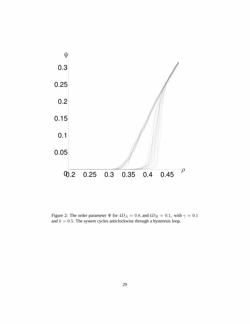
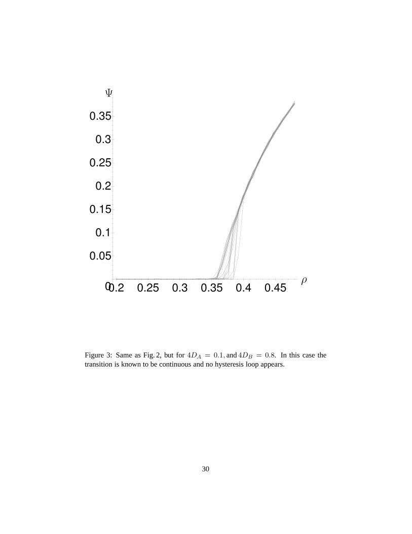
This whole procedure constitutes a simulation cycle. In this way we produced21 cycles with different pseudo-random numbers. Figures 2 and 3 show the result-ing order parameter curves in two different cases: in Figure2 we haveDB < DA

and the system cycles counterclockwise through a hysteresis loop, signalling the

14

occurrence of a first order transition. In Figure 3 exactly the same simulation pro-cedure does lead to some dispersion in the order parameter curves, but not to aclearcut hysteresis loop; in this case the transition is known to be continuous.

5 Perturbative calculation of the equation of state

5.1 One-loop perturbation expansion

In this section we determine the one-loop equation of state.We start from thedynamic functional of Eq. (7), in which we have included a particle source term−∫

ddrdt λh(r , t)ψ(r , t). The equations of motion for the fields are

0 =δS

δm= ∂tm− λ(ρ∇2m+ σ∇2ψ) + 2λρ∇2m (49)

0 =δS

δψ= ∂tψ + λ(τ −∇2 + fm)ψ +

λg

2ψ2 − λgψψ − λh (50)

Note that the source term is not necessarily constant. Equations (49) and (50) arevalid when they are inserted in averages. Taking the averages of (49) and (50) wefind for the densitiesM(r ) = 〈m(r , t)〉 andΨ(r ) = 〈ψ(r , t)〉 in a stationary statethe exact equations

ρ∇2M(r ) + σ∇2Ψ(r) = 0 (51)[

τ −∇2 + fM(r) +g

2Ψ(r)

]

Ψ(r) + fCmψ(r ) +g

2Cψ(r ) = h(r ) (52)

with the correlation functions

Cmψ(r) = 〈(m−M(r )) (ψ − Ψ(r ))〉 Cψ(r ) =⟨

(ψ − Ψ(r))2⟩

. (53)

¿From equation (51) it follows that

M(r ) = −σρ

Ψ(r ) + c(r ) (54)

wherec(r ) is a harmonic function (∇2c = 0). Here we assume thatc is constant.(It has to be constant in the thermodynamic limit if bothM and Ψ are free ofsingularities and finite forr → ∞.) If

∫

V ddrm(r , t) = 0 (which can always beachieved by a shift ofτ ) we get

c =σ

ρV

∫

VddrΨ(r) (55)

whereV denotes the volume of the system.

15

The mean field equation for the profile reads

[

τ + fc−∇2 +g

2Ψmf (r )

]

Ψmf (r) = h(r ) (56)

whereg = g − 2σf/ρ. Equation (56) shows that stability of the mean field theoryrequires thatg ≥ 0. For negativeg higher powers inψ have to be taken intoaccount in the functionalS. We first consider an external fieldh which is constantwithin a sphere of radiusR and vanishes forr > R. For simplicity we take thethermodynamic limitV,R → ∞ in such a way thatRd/V → 0. In this case theregion outside the sphere acts as a reservoir for the homogeneous mode of the fieldm, and in (56) we can setc = 0 for τ > 0.

To calculate the one-loop correction to the equation of state we shift the fieldsψ andm by their average values and obtain

S[m,M +m; ψ, ψ + Ψ] = S0[ψ; Ψ] + SG[m,m; ψ, ψ; Ψ] + SI [m; ψ, ψ] (57)

with

S0[ψ; Ψ] =

∫

dt∫

ddrλψ[(

τ −∇2 +g

2Ψ)

Ψ − q]

(58)

where we have kept the fullr -dependence ofΨ and expressedM in terms ofΨ.The Gaussian part ofS reads

SG[m,m; ψ, ψ; Ψ] =

∫

dt∫

ddr[

m(

∂tm− λ∇2(ρm+ σψ))

− λρ(∇m)2

ψ(

∂tψ + λ(

τ −∇2 + (g − σf/ρ)Ψ)

ψ + λfΨm)

− 1

2λgΨψ2

]

(59)

and the interaction part is

SI [m; ψ, ψ] =

∫

dt∫

ddrλ

[

fmψψ +1

2ψ(gψ − gψ)ψ

]

. (60)

The Gaussian propagatorsGψ = 〈ψψ〉,Gm = 〈mm〉,Gmψ = 〈mψ〉 andGψm =〈ψm〉 follow from (59). They satisfy the differential equations

(

∂t + λ(τ −∇2))

Gψ(r , r ′; t− t′) + λfΨGmψ(r , r ′; t− t′) = δ(d)(r − r ′)δ(t − t′) (61)(

∂t − λρ∇2)

Gmψ(r , r ′; t− t′) − λσ∇2Gψ(r , r ′; t− t′) = 0 (62)(

∂t − λρ∇2)

Gm(r , r ′; t− t′) − λσ∇2Gψm(r , r ′; t− t′) = δ(d)(r − r ′)δ(t − t′) (63)(

∂t + λ(τ −∇2))

Gψm(r , r ′; t− t′) + λfΨGm(r , r ′; t− t′) = 0 (64)

16

with τ = τ + (g − σf/ρ)Ψ. The Gaussian propagators can be used to determinethe equal time correlation functions (53) to lowest nontrivial order:

Cmψ(r) =

∫ ∞

0dt∫

ddr′[

λgΨ(r ′)Gmψ(r , r ′; t)Gψ(r , r ′; t)

+2λρ(

∇′Gm(r , r ′; t)) (

∇′Gψm(r , r ′; t))]

(65)

Cψ(r ) =

∫ ∞

0dt∫

ddr′[

λgΨ(r ′)(

Gψ(r , r ′; t))2

+ 2λρ(

∇′Gψm(r , r ′; t))2]

. (66)

For constantΨ the equations (61)-(64) can easily be solved by Fourier transforma-tion. In this way one obtains for the fluctuation term in the equation of state (52)

fCmψ +g

2Cψ =

∫

q

Ψ

τ + (1 + ρ)q2

[

1

4gg − f2 +

g(gρq2 + 2f2Ψ)

4(τ ′ + q2)

]

(67)

with τ ′ = τ − σfΨ/ρ. After dimensional regularization the momentum integralbecomes

fCmψ +g

2Cψ = − AεΨ

2ε(1 + ρ)

(

τ

1 + ρ

)1−ε/2 [

gg − 4f2 + ggρ+1 + ρ

τg(gρτ ′ − 2f2Ψ)

+ε

2

(1 + ρ)2τ ′

τ

g(gρτ ′ − 2f2Ψ)

τ − (1 + ρ)τ ′ln

(1 + ρ)τ ′

τ+ O(ε2)

]

(68)

whereAε = (4π)−d/2Γ(1 + ε/2)/(1 − ε/2).

5.2 Renormalized equation of state

In order to absorb theε-poles in the equation of state (52,68) into a reparametriza-tion of coupling constants and fields we make use of the renormalized quantitiesψR, λR, ρR etc. introduced in Eqs. (11,12).

The renormalized quantities satisfy the equation of state

hR = ΨR

{

τR +gR

2ΨR +

1

4(1 + ρR)

[

((1 + ρR)u− 4v − 2w)τR

1 + ρR

lnµ−2τR

1 + ρR

(69)

+(ρRu− 2w)τ ′R − 2vgRΨR

τR − (1 + ρR)τ ′R

(

τR lnµ−2τR

1 + ρR

− (1 + ρR)τ′R ln(µ−2τ ′R)

)]}

wheregR = gR − 2fR/ρR, τR = τR + (gR − fR/ρR)ΨR andτ ′R = τR + gRΨR are therenormalized counterparts ofg, τ andτ ′, respectively. ForfR = v = w = 0 werecover the one loop-equation of state for directed percolation [20]. To simplify

17

the writing in equation (69) the geometrical factorAε, the momentum scaleµ andσR have been absorbed into a rescaling ofΨR andhR, i.e.

A−1/2ε µε/2σRΨR → ΨR andA−1/2

ε µε/2σRhR → hR (70)

Hereafter we will drop the index “R” since only renormalizedquantities will beused.

6 Flow equations

6.1 Renormalization group for the equation of state

The renormalizability of the field theory implies a set partial differential equationsfor the vertex functions. These are the renormalization group equations whichfollow from the independence of the bare vertex functions onthe momentum scaleµ. To investigate the equation of state in the critical regionwe need the one-pointvertex functionΓ(1,0) which is (up to a factorλ) equal toh(τ,Ψ;u, v,w, ρ;µ). Therenormalization group equation forh reads[

µ∂

∂µ+ βu

∂

∂u+ βv

∂

∂v+ βw

∂

∂w+ βρ

∂

∂ρ+ κτ

∂

∂τ+ ζ − γ

]

h(τ,Ψ;u, v,w, ρ;µ) = 0

(71)

with theβ-functions given in Sec. 2.

6.2 Scaling form of the equation of state

The renormalization group equation Eq. (71) can be solved bycharacteristics withthe result

h(τ,Ψ;u, v,w, ρ;µ) = Yh(ℓ)−1(µℓ)2+d/2

×h(

Yτ (ℓ)(µℓ)−2τ, (µℓ)−d/2Ψ;u(ℓ), v(ℓ), w(ℓ), ρ(ℓ); 1

)

(72)

where

da(l)d ln ℓ

= βa(u(ℓ), v(ℓ), w(ℓ), ρ(ℓ)) for a = u, v,w, ρ (73)

d lnYτ (ℓ)

d ln ℓ= κ(u(ℓ), v(ℓ), w(ℓ), ρ(ℓ)) (74)

d lnYh(ℓ)

d ln ℓ= γ(u(ℓ), v(ℓ), w(ℓ), ρ(ℓ)) − ζ(u(ℓ), v(ℓ), w(ℓ), ρ(ℓ)) (75)

18

are the characteristics with the initial conditionsu(1) = u, v(1) = v, w(1) = w,ρ(1) = ρ andYτ (1) = Yh(1) = 1. Some solutions of the flow equations (73) aredepicted in figure 4. For small initial values ofw ∝ DA − DB the trajectoriesfirst approach the unstable manifold of the symmetric fixed point (w = 0) beforethey flow away. The unstable manifold leaves the stability region of the mean fieldtheory (g > 0, or u − 2w/ρ > 0) at the point(u⋆, v⋆, w⋆, ρ⋆). The numericalsolution of the flow equations yieldsu⋆ = 12.32ε, v⋆ = 2.104ε, w⋆ = 22.11ε,andρ⋆ = 3.589. The intersection point of the unstable manifold with the stabilityedge g = 0 is of special interest since the perturbatively improved mean fieldtheory should be a good approximation for smallg (as will be discussed in the nextsection). Therefore the phase transition for very smallw > 0 is governed by theequation of state at the point(u⋆, v⋆, w⋆, ρ⋆). In the following we shall denote byℓ⋆the value of the flow parameter at whichu(ℓ⋆)−2w(ℓ⋆)/ρ(ℓ⋆) = 0 and byξ⋆ = eℓ⋆

the related length scale. One can identifyξ⋆ with its heuristic counterpart definedin Eq. (43). The flow equations are too complicated to be solved analytically forall ℓ, however it is possible, using scaling arguments, to predict that, asσ → 0+,ξ⋆ ∝ σ2/γs , a form also proposed in Eq. (46).

7 A first-order transition for DA > DB

In this section we study the mean field equation of state with the one-loop fluctua-tion correction (69) for small values of the couplingg ≪ g. Our motivation is ananalogy of our reaction diffusion system with spin systems with cubic anisotropy.Using a modified Ginzburg criterion for systems with cubic anisotropy Rudnick [2](see also [3]) has shown that the fluctuation corrected mean field approximationshould give reliable results if the values of the coupling coefficients are close to thestability edge of the mean field theory. In the case of the reaction diffusion systemwith DA > DB the stability edge is given byg = 0.

Now assume that we start with a very small value of the couplingw and choosethe flow parameterℓ = ℓ⋆ in (72). After theℓ-dependent prefactorsYτ (ℓ⋆)ℓ−2

⋆

etc. have been asborbed into a rescaling ofτ , h, andΨ the improved mean fieldequation of state takes the simple form

h = Ψ

[

τ +u⋆ − 4v⋆

4(1 + ρ⋆)2

(

τ +g⋆2

Ψ)

lnτ + g⋆Ψ/2

µ2(1 + ρ⋆)+ O(two-loop)

]

(76)

with (u⋆ − 4v⋆)/(4(1 + ρ⋆)2) = 0.04635 ε > 0.

In the limith→ 0+ the absorbing state withΨ = 0 is a solution of the equation

19

of state for allτ . Forτ < τspinod with

τspinod = µ2e−1 u⋆ − 4v⋆4(1 + ρ⋆)

= O(ε) (77)

there is also a solution withΨ > 0 and∂Ψ/∂h > 0 (see figure 5). To see thisone should anticipate that when the order parameter is of theorder of its value atτspinod one has

τspinodg⋆Ψ

= O(ε) (78)

and to leading order the reasoning is carried out on

h = Ψ

[

τ +u⋆ − 4v⋆

4(1 + ρ⋆)2g⋆2

Ψ lng⋆Ψ

2(1 + ρ⋆)µ2

]

(79)

Solving the latter equation forh = 0 and ∂h∂Ψ = 0 yields, to leading order inε,

Ψspinod =8(1 + ρ⋆)

2

u⋆ − 4v⋆

τspinodg⋆

, τspinod = µ2e−1 u⋆ − 4v⋆4(1 + ρ⋆)

(80)

which a posteriori justifies working on the approximation Eq. (79). Since the sus-ceptibility χ = ∂Ψ/∂h (the response of the order parameter to particule injection)is positive the new solution is at least metastable for allτ < τspinod. The openquestion is for which range ofτ the solution is stable, i.e., stable also with respectto nucleation processes. If we could derive the equation of state from a free energythis question would be easy to answer: a metastable solutionis alocal minimum ofthe free energy while a stable solution is aglobal minimum. However, since thereis no free energy for the reaction diffusion system we have tolook for a differentstability criterion, e.g. the form of density profiles. By analogy with equilibriumsystems we expect that the solution withΨ > 0 is stable below a coexistence“temperature” (in our case we should talk about a coexistence density)τcoex with0 < τcoex < τspinod.

8 Deriving τcoex from a density profile

If τ is so large that equation (76) has only the trivial solutionΨ = 0 the densityΨ(r ) generated by a local sourceh(r ) decays rapidly with increasing distance fromthe region in whichh(r ) is nonzero. Consider for instance a plane particle sourcewith

h(r ) = h0δ(r⊥) (81)

20

wherer⊥ is the coordinate perpendicular to the source. For simplicity assumethat h0 → ∞. For larger⊥ the profile [i.e., the solution of (52)] will becomeindependent ofr⊥ and tend to either (a)Ψ = 0 if τ is sufficiently large or (b) thenonzero solution of (76). In the thermodynamic limit the whole profile Ψ(r) isuniquely determined by the sourceh(r ) sinceΨ has to be finite forr⊥ → ±∞. Inthe case (a) we can conclude thatτ > τcoex whereas (b) occurs forτ < τcoex.

In order to calculate a density profile perturbatively one usually starts with themean field profile and assumes that the fluctuation corrections are small (of theorder ε, say). In the present case this procedure would not lead to the desiredresult since the nonzero solution of the equation of state for τ < τspinod is of theorderε0. It can therefore not be derived as a small correction toΨmf . Instead wehave to compute theequation for the density profileperturbatively and then studythe asymptotic behavior of its solutions. This means that weneed the correlationfunctionsCmψ(r ; {Ψ}) andCψ(r ; {Ψ}) in equation (52) for a general functionΨ(r ). Of course, we cannot compute these functions exactly but itis possible toderive a systematic gradient expansion forCmψ andCψ.

We first compare the leadingε-orders in equation (52) (withM = −σΨ/ρ):Since we expect that the coexistence point to be located in the parameter range0 < τ ≤ τspinod = O(ε) we may setτ = O(ε). The limit of a very weak firstorder transition is governed by the point(u⋆, v⋆, w⋆, ρ⋆) which means thatg = 0and that the combinationfCmψ + g

2Cψ is of orderO(ε). Comparing the terms onthe l.h.s. of (52) therefore yields(∇2Ψ)/Ψ = O(ε), i.e. gradients ofΨ may beconsidered as small quantities when we calculateCmψ andCψ. Using the Taylorseries

Ψ(r ′) = Ψ(r) +∞∑

N=1

1

N !

∑

α1···αN

(r′ − r)α1. . . (r′ − r)αN

∂α1. . . ∂αN

Ψ(r ) (82)

for the profile one arrives at a gradient expansion forCmψ andCψ of the form

Cψ(r , {Ψ}) = Cψ(Ψ(r )) +

∞∑

N=1

1

N !

∑

α1···αN

Cψ;α1···αN(Ψ(r ))∂α1

. . . ∂αNΨ(r).

(83)

At leading order inε only the first term on the r.h.s. of (83) contributes, i.e., wemaysimply replaceΨ in (68) by the profileΨ(r) and use the result in equation (52).After application of the renormalization group as before and absorbingℓ-dependentprefactors the equation for the profile becomes

h(r ) = Ψ(r)[

τ +u⋆ − 4v⋆

4(1 + ρ⋆)2

(

τ +g⋆2

Ψ(r))

lnτ + g⋆Ψ(r)/2µ2(1 + ρ⋆)

]

−∇2Ψ(r) + O(ε2).

(84)

21

In order to extend this result to the next order inε one has to (i) computeCmψ andCψ for constantΨ to two-loop order and (ii) take into account the∇2Ψ-correctionin the gradient expansion (83) to one-loop order. In this waythe∇2Ψ-term in (84)may receive aΨ-dependent correction.

Forh(r ) = h0δ(r⊥) Eq. (84) can be integrated once after multiplication of bothsides withΨ′(r⊥). In figure 6 the result is depicted for various values ofτ . Thereis a valueτcoex < τspinod such that the profile does not tend to zero forr⊥ → ±∞if τ ≤ τcoex. As discussed aboveτcoex is the coexistence point below which theactive phase becomes a stable solution of the equation of state. Again one workswith Eq. (79). In practice one has to solve the system composed of Eq. (79) withh = 0 along with its integrated counterpart

0 =τcoex

2Ψ2coex +

u⋆ − 4v⋆24(1 + ρ⋆)2

g⋆Ψ3coex

[

lng⋆Ψcoex

2µ2(1 + ρ⋆)− 1

3

]

(85)

The explicit calculation yieldsΨcoex = 12(1+ρ⋆)2τcoex

(u⋆−4v⋆)g⋆(which also justifies the use

of the simplified equation of state Eq. (79)), with

τcoex = µ2e−2/3 u⋆ − 4v⋆6(1 + ρ⋆)

= 0.93τspinod. (86)

τcoex/τspinod is not a universal number, but the susceptibility ratioχ+/χ− with

χ+ = limh→0

∂Ψ

∂h

∣

∣

∣

∣

Ψ=0,τcoex

χ− = limh→0

∂Ψ

∂h

∣

∣

∣

∣

Ψ>0,τcoex

(87)

is universal. To one-loop order one finds

χ+

χ−=

1

2+ O(ε) (88)

This result is analogous to the universality of the magneticsusceptibility ratiofound by Rudnick [2] and Arnold and Yaffe [3].

9 Conclusions and prospects

9.1 A heuristic functional for the steady state phase diagram

In this paragraph we would like to builda posteriori a functional of the orderparameter fieldΨ(r) describing the phase diagram in the stationary state of the

22

system. We emphasize that the following is only valid to one loop order. We defineF [Ψ] by

F [Ψ] =

∫

ddr

[

1

2(∇Ψ)2 +

∫ Ψ(r)

0dψ Γ(1,0)[0, ψ]

]

(89)

By construction of courseδFδΨ = 0 is equivalent to the equation of state Eq. (79).It is instructive to plotF as a function ofΨ for various values ofτ (see figure 7).There it appears possible to deduce the phase diagram from the global minima ofF [Ψ]. However the route leading to the functionalF [Ψ] follows a series of field-theoretic detours. The suggestive notationF , which reminds of a free energy (inthe equilibrium statistical mechanics sense) is however misleading. For instanceit could not be used as an effective Landau hamiltonian for the calculation of aGibbs partition function describing fluctuations directlyin the steady state. Thisfunctional is a remarkably compact and intuitive way of summarizing the propertiesof the steady state phase diagram. In particular the spinodal point τspinod appears asthe point below whichF develops a second minimum. Belowτcoex that minimumbecomes the global minimum. To one loop order the equilibrium vocabulary cantherefore be used carelessly.

9.2 Summary

In the course of this work we have elaborated a phenomenological description ofa fluctuation-induced first-order transition taking place in a nonequilibrium steadystate, the first one of this sort. We have in parallel applied field-theoretic tech-niques to derive an effective (renormalization-group improved) equation of statethat incorporates those fluctuations. This yields a PDE for the order parameterin the steady state. Performing a study of the stability (against space fluctuationsof the order parameter) of the solutions of this PDE has led usto a complete de-scription of the phase diagram. We have identified in this nonequilibrium situationa concept analogous to the point of spinodal decomposition consistent with ourphenomenological description.

9.3 Possible applications

Among the many nonequilibrium systems that appear in the literature, driven dif-fusive systems lend themselves to an analytic treatment by techniques similar tothose of the present article [21]. In a number of such systemsthough, a significantportion of the phase space (in terms of control parameters) escapes conventionalanalysis. In some cases we believe that the reason is the occurrence of fluctuation-induced first order transition, such as in [9] or [8]. It wouldbe quite interesting to

23

see how both the technical argument and the heuristics can beextended to thosesystems. This will be the subject of future work.

Acknowledgments: K. O. would like thank the Sonderforschungsbereich 237 ofthe DFG for support and H. K. Janssen for interesting discussions.

24

Appendix

There are two ways to proceed in order to obtain the equation of state to one-looporder. In this appendix we follow the route familiar from static critical phenomena.We use the action Eq. (8) as the starting point of our analysis. The first task is todetermine the one-loop expression of the effective potential Γ.

Γ[ψ, ψ] = S[ψ, ψ] +1

2

∫

ddq(2π)d

dω2π

ln detS′′(q, ω)[ψ, ψ] (90)

with the matrixS′′ defined by

S′′(q, ω) =

(

δ2Sδψ(−q,−ω)δψ(q,ω)

δ2Sδψ(−q,−ω)δψ(q,ω)

δ2Sδψ(−q,−ω)δψ(q,ω)

δ2Sδψ(−q,−ω)δψ(q,ω)

)

(91)

S′′11(q, ω) = λ(q2 + τ) − iω − λgΨ − λ2σfΨ

q2

q2 − iω− 2

(λf)2q2

q4 + ω2Ψψ (92)

S′′12(q, ω) = −2(λf)2q2

q4 + ω2Ψ2 − λgΨ (93)

S′′21(q, ω) = −2(λf)2q2

q4 + ω2ψ2 − 2

λ2σfq4

q4 + ω2ψ + λgψ (94)

S′′22(q, ω) = λ(q2 + τ) + iω − λgΨ − λ2σfΨ

q2

q2 + iω− 2

(λf)2q2

q4 + ω2Ψψ (95)

For a homogeneous source termh the equation of state for a homogeneous orderparameterΨ now follows from the requirement that

δΓ

δψ[0,Ψ] = 0 (96)

It is a tedious but straighforward task to find the one-loop correction toΓ(1,0) in theform of an integral over momentum and frequency. Writing

Γ(1,0)[ψ = 0, ψ = Ψ] = −λh+ λΨ(τ +1

2gΨ) + δΓ(1,0) (97)

one finds

δΓ(1,0) = − λ2

∫

ddq(2π)d

dω2π

(

q2 + τ − 1

2gΨ

)

×(

g(q4 + ω2) + 2λf2q2Ψ)

×[(

ω2 − iAω −B) (

ω2 + iAω −B)]−1

(98)

25

where we have defined the auxiliary variables

A ≡ (λ+ 1)q2 + λτ , B ≡ q2λ(q2 + τ ′) (99)

Upon using the following integration formulas,∫

dω2π

1

ω2 ± iAω −B= 0,

∫

dω2π

1

|ω2 ± iAω −B|2 =1

2AB(100)

Eq. (98) simplifies into

δΓ(1,0) = − λ

2

∫

ddq(2π)d

[

(q2 + τ − 1

2gΨ)

(

g(q2 +τ ′

1 + ρ) +

2f2

1 + ρΨ

)]

×[

(q2 + τ ′)(q2 +τ

1 + ρ)

]−1

(101)

The above expression can be cast in a form suitable to performtheq-integrals:

δΓ(1,0) = − 1

2λg

∫

ddq(2π)d

+λΨ

4((1 + ρ)τ ′ − τ)

[

g(ρg − 2σf)τ ′ − 2f2gΨ]

∫

ddq(2π)d

1

q2 + τ ′

+λΨ

4(1 + ρ)((1 + ρ)τ ′ − τ )

[

2gσf τ − (1 + ρ)ggσf

ρΨ

− 4ρf2τ + 2g(1 + ρ)f2Ψ

]

∫

ddq(2π)d

1

q2 + τ1+ρ

(102)

We use dimensional regularization to compute the momentum integrals:∫

ddq(2π)d

1

q2 + τ ′= −2

ετ ′1−ε/2Aε,

∫

ddq(2π)d

1

q2 + τ1+ρ

= −2

ε

(

τ

1 + ρ

)1−ε/2

Aε

(103)

In terms of renomalized quantities the equation of state hasthe form

hR =ΨR

{

τR +gR

2ΨR +

1

4(1 + ρR)

[

((1 + ρR)u− 4v − 2w)τR

1 + ρR

lnµ−2τR

1 + ρR

+(ρRu− 2w)τ ′R − 2vgRΨR

τR − (1 + ρR)τ ′R

(

τR lnµ−2τR

1 + ρR

− (1 + ρR)τ′R ln(µ−2τ ′R)

)]}

(104)

which is Eq. (69).

26

Figures

27

β = 1 − ε

32+ O(ε2)β = 1

DA < DB

〈ψ(t = +∞)〉

τ DA > DB τDA = DBτ

Figure 1: Phase diagram in the(τ, ψ(t = ∞)) plane (the ordinate is the steady-state density ofB particles) forλ > 1, λ = 1 and a conjecture forλ < 1. Alsoshown is the order parameter exponentβ.

28

0.450.40.350.30.250.2

0.3

0.25

0.2

0.15

0.1

0.05

0

Ψ

ρ

Figure 2: The order parameterΨ for 4DA = 0.8, and4DB = 0.1, with γ = 0.1andk = 0.5. The system cycles anticlockwise through a hysteresis loop.

29

0.450.40.350.30.250.2

0.35

0.3

0.25

0.2

0.15

0.1

0.05

0

Ψ

ρ

Figure 3: Same as Fig. 2, but for4DA = 0.1, and4DB = 0.8. In this case thetransition is known to be continuous and no hysteresis loop appears.

30

gg

DA < DB DA > DB

w

Figure 4: Flow diagram in the(gg, w) plane. The leftmost black dot stands fortheDA < DB fixed point while the one lying on thew = 0 axis stands for thesymmetricDA = DB fixed point. They both describe second order transitions.Typical trajectories have been drawn. Those starting closeto the symmetric fixedpoint but with an initial positivew eventually flow away from the symmetric fixedpoint.

31

Ψ

h

τ < τspinod

τ = τspinod

τ > τspinod

Figure 5: Sketch of the functionh(τ,Ψ), Eq. (76).

32

τ = τspinod

Ψ(r⊥)

τ = τcoex

Ψ′(r⊥)

Figure 6: Derivative of the density profileΨ′(r⊥) as a function ofΨ(r⊥) for τ ≥τcoex. The boundary condition atr⊥ = 0+ is given byΨ′(0) = −h0/2.

33

τ < τcoex

F [Ψ]

Ψ

τcoex

τ > τspinod τspinod τspinod > τ > τcoex

Figure 7: F [Ψ] as a function ofΨ for decreasing values ofτ . We identify thespinodal point as the value ofτ below whichF develops a local nonzero minimumand the coexistence point as the point at which the two minimabecome degenerate.

34

References

[1] E. Domany, D. Mukamel and M. Fisher,Phys. Rev. B15 (1977) 5432.

[2] J. Rudnick,Phys. Rev. B18 (1978) 1406.

[3] P. Arnold and L. G. Yaffe,Phys. Rev.D 55 (1997) 7760.

[4] J.-H. Chen, T. C. Lubensky and D. R. Nelson,Phys. Rev. B17 (1978) 4274.

[5] F. Y. Wu, Rev. Mod. Phys.54 (1982)

[6] S. Coleman and E. Weinberg,Phys. Rev. D7 (1973) 1883.

[7] B. Derrida, Phys. Rep.301(1998) 65.

[8] G. Korniss, B. Schmittmann and R. K. P. Zia,J. Stat. Phys.86 (1997) 721.

[9] H. K. Janssen and B.Schmittmann,Z. Phys. B64 (1986) 503.

[10] R. Kree, B. Schaub and B. Schmittmann,Phys. Rev. A39 (1989) 2214.

[11] F. van Wijland, K. Oerding and H. J. Hilhorst,Physica A251(1998) 179.

[12] L. Peliti, J. Physique46 (1985) 1469.

[13] H. K. Janssen,Z. Phys.B 42 (1981) 151.

[14] H. K. JanssenZ. Phys.B 23 (1976) 377.

[15] C. De Dominicis,J. Physique (Paris)C 37 (1976) 247.

[16] I. D. Lawrie and S. Sarbach, inPhase transitions and critical phenomena,Vol. 9, C. Domb and J. L. Lebowitz eds. (Academic Press, New York, 1984).

[17] L. Landau and E. Lifshitz,Cours de physique theorique, tome X : Cinetiquephysique(Mir, Moscou, 1989).

[18] R. Bausch, H. K. Janssen and H. Wagner,Z. Phys.B 24 (1976) 113.

[19] H. K. Janssen in:From Phase Transitions to Chaos, Topics in Modern Statis-tical Physics, G. Gyorgyi, I. Kondor, L. Sasvari and T. Tel eds. (World Scien-tific, Singapore, 1992) pp 68-91.

[20] H. K. Janssen,U. Kutbay and K. Oerding,J. Phys. A: Math. Gen.32 (1999)1809.

35

[21] B. Schmittmann and R. K. P. Zia,Phase transitions and critical phenomena,Vol. 17, C. Domb and J. L. Lebowitz eds. (Academic Press, New York, 1995).

[22] P. C. Martin, E. D. Siggia and H. A. Rose,Phys. Rev.A 8 (1973) 423.

36