This article appeared in a journal published by Elsevier. The attachedcopy is furnished to the author for internal non-commercial researchand education use, including for instruction at the authors institution

and sharing with colleagues.

Other uses, including reproduction and distribution, or selling orlicensing copies, or posting to personal, institutional or third party

websites are prohibited.

In most cases authors are permitted to post their version of thearticle (e.g. in Word or Tex form) to their personal website orinstitutional repository. Authors requiring further information

regarding Elsevier’s archiving and manuscript policies areencouraged to visit:

http://www.elsevier.com/copyright

Author's personal copy

Physica A 391 (2012) 170–179

Contents lists available at SciVerse ScienceDirect

Physica A

journal homepage: www.elsevier.com/locate/physa

Detecting switching points using asymmetric detrended fluctuationanalysisMiguel A. Rivera-Castro a, José G.V. Miranda a, Daniel O. Cajueiro b,c, Roberto F.S. Andrade a,c,∗

a Instituto de Física, Universidade Federal da Bahia, BA 40210-340, Brazilb Department of Economics – University of Brasilia, DF, 70910-900, Brazilc National Institute of Science and Technology for Complex Systems, Brazil

a r t i c l e i n f o

Article history:Received 5 May 2011Received in revised form 5 July 2011Available online 30 July 2011

Keywords:Switching pointsAsymmetric fluctuationsLocal detrended analysisFinancial series

a b s t r a c t

This work uses the concept of Asymmetric Detrended Fluctuation Analysis (A-DFA) toinvestigate and characterize the occurrence of trend switching in financial series. A-DFAintroduces two new roughness exponents, H+ and H−, which differ from the usual oneH by separately taking into account contributions to the fluctuations according to whetherthe local trend is, respectively, upward or downward. The developedmethodology requiresthe evaluation of local values of H(t),H+(t), and H−(t), by restricting the size of thelargest window around the value t . We show that H+(t) and H−(t) behave differentlyin the neighborhoods of switching points (SPs) where trends change sign. Properly takendifferences between shifted local values of H(t),H+(t), and H−(t) allow to identify andcharacterize SP’s. Tests with Weiertrasse functions, isolated peaks, and actual financialseries are presented, supporting the validity of the proposed method.

© 2011 Elsevier B.V. All rights reserved.

1. Introduction

Within the broad framework provided by statistical physics, it has been recognized that financial markets are typicalcomplex systems, with a large number of agents with different perspectives and conflicting interests, affected by largenumber of random, time dependent information input arising from any country in the world [1–3]. The fact that the forcesacting on the market are of different nature and that small disturbances may result in large effects is responsible for thestochastic nature of this system and for its complexity. The large amount of actual data provided by the market recordstogether with their importance for everyone’s daily life have turned financial markets into paradigmatic systems, beingcurrently applied to develop useful tools to measure, understand and, if possible, predict the dynamics of complexity [4–6].

Price fluctuations in stock market records constitute primary economic information source [7,8] that have beenthoroughly investigated for the purpose of understanding specific features of economic dynamics, among which the trendfor persistent rise or fall of prices changes. Preis and Stanley [9–12] have enlarged this perspective for any generic complexsystems, introducing the concept of switching points (SPs) to characterize such events in a more precise way, by stating thatsuch trend changes occur in an abrupt and almost discontinuous way. In the specific case of financial markets, switchingevents creating upward trends (‘‘bubbles’’) and downward trends (‘‘financial collapse’’) have been fairly common in the pastthree decades [13,4,5]. This change occurs at scale times ranging frommacroscopic bubbles persisting for hundreds of daysto microscopic bubbles persisting for only seconds.

∗ Corresponding author at: Instituto de Física, Universidade Federal da Bahia, BA 40210-340, Brazil. Tel.: +55 71 32337518.E-mail addresses:marc@ufba.br (M.A. Rivera-Castro), vivas@ufba.br (J.G.V. Miranda), danielcajueiro@unb.br (D.O. Cajueiro), randrade@ufba.br

(R.F.S. Andrade).

0378-4371/$ – see front matter© 2011 Elsevier B.V. All rights reserved.doi:10.1016/j.physa.2011.07.009

Author's personal copy

M.A. Rivera-Castro et al. / Physica A 391 (2012) 170–179 171

According to the original definition, an SP event, at a specific instant of time ti within a complex system record y(t), isidentified by a very large value of the return variance within a local window around ti [10]. The magnitude of such eventscan vary over many time scales that depend on a precise definition of ‘‘large’’ and of the window width L and, as such, acomprehensive approach for SP deserves careful analyses. On the other hand, we think it is important to investigatewhetherother features present in the records can be used to detect SPs. In thiswork, we develop an approach for SP identification andcharacterization based on the asymmetric detrended fluctuation analysismethod [14] (A-DFA). It has been devised to identifydifferent fluctuation properties of presumed non-stationary series, by identifying and separating fluctuation contributionsaccording to the upward or downward character of the local trend. If the fluctuations are casted into two groups accordingto different trends at all scales, it is possible to define two new scaling exponents, say H+ and H−. If the series is symmetricwith respect to the trends, both H+ and H− are equal to the usual roughness (or Hurst) exponent H . If this property is notobserved, the method assigns a measurable asymmetric character to the series.

To extend this idea for SP identification, we develop a local A-DFA evaluation procedure. Namely, we couple A-DFA witha sliding window procedure, which amounts to evaluating local exponents H(t),H+(t) and H−(t). As we will discuss, ithappens that the set of three local roughness exponents allows to characterize, in qualitative and quantitative ways, theemergence of sudden changes in the time records that we identify as SPs. The method happens to be robust with respectto the width of the sliding window, provided it remains small enough to be considered local and large enough to includesufficient points for the DFA analysis.

This paper is further organized as follows. In Section 2, we indicate the most important steps for the A-DFA procedure, insuch away to provide an easy-to-follow receipt on how the results have actually been obtained. Section 3 is divided into twosubsections, where we discuss, respectively, results for series generatedwith specific algorithmswarranting specific scalingproperties, and on price series from stock markets. Finally, Section 4 presents our concluding remarks and discussions.

2. Local asymmetric detrended fluctuation analysis

DFA is a reliablemethod for the evaluation of the roughness exponentH of a stationary random time series. In its originalandmost used form [15,16], linear trends are eliminated from the series by calculating fluctuations around the best straightline segment in a box of length n. Generalized versions of the original idea have been proposed, in which trends representedby higher polynomial order q (DFAq) can be eliminated [17] or, alternatively, detrended multi-fractal analyses of non-stationary series can be performed [18]. In recent works [19,20], the idea of detrending was enlarged in a different context,namely, taking into account the mutual influence of two time series by defining the detrended cross-correlation analysis.It has also been shown that, by working with polynomials of degree q, periodic trends in data have been eliminated in thecross-correlation analysis [21]. The common feature in any detrending algorithm is quite useful as it allows to eliminatetrends in many scale regions that are mostly reflecting the global adjustment of the system to some external parametervariations rather than reflecting the intrinsic dynamic properties of the system.

If we start with a series of equidistant time increments {x(t)}, t = 1, . . . ,N , we can obtain the path (or the profile)

y(t) =

t−j=1

x(t). (1)

The entire interval [1,N] can be divided into a series ofMn boxes of length n, not necessarily self-excluding. Each of suchboxes receives a label (m, n),m = 1, . . . ,Mn. In our calculations, we considered a certain level of overlap between the boxesfor the purpose of increasing the number of boxes where the method is applied and, hence, to improve the statistics.

To evaluate themagnitude of fluctuations in the box (m, n) and, concomitantly, eliminate the trendof order q, we considerthe difference

ys(t) = y(t) − pq(t; (m, n)), (2)

where pq(t; (m, n)) represents the polynomial of order q that minimizes the sum of ys(t)2 when t spans all points of theconsidered box. To be more precise, we consider the residue

f (m, n) =1n

Imax(m,n)−j=Imin(m,n)

y2s (j), (3)

where Imin(m, n) and Imax(m, n) are the lower and upper limit of the (m, n) box. When q = 0, f (m, n) corresponds to theroughness functionW (m, n) of the (m, n) box. Subsequently, we have the average

F(n) =

1Mn

Mn−m=1

f (m, n)

1/2

, (4)

which expresses the average detrended roughness at length scale n of the entire profile. If the original series presents long-range correlations, it is expected that the values of F(n) follows a power law

F(n) ∼ nH , (5)

Author's personal copy

172 M.A. Rivera-Castro et al. / Physica A 391 (2012) 170–179

where the roughness exponent H = 1 − γ /2 is related to the exponent describing the decay of the correlation functionC(j) = ⟨y(t)y(t + j)⟩ ∼ j−γ , and ⟨ ⟩ represents the series average. In the current work, as we proceed with the investigationof economic and financial data, y(t) represents the logarithm of the price or the market index in the original series.

The A-DFAq variant proposed by Alvarez-Ramirez et al. [14] aims to characterize correlations in non stationaryasymmetric time series, so that two further exponents H+ and H− can inform on the scaling properties when the seriestrends are upwards or downwards. The basic idea is to cast the sums in (3) into two classes according to the trend propertyof the (m, n) box. For this purpose, some extra stepsmust be added to usual DFAq framework sketched above. Sowe consideralso

xs(t) = x(t) − r1(t; (m, n)), (6)

where r1(t; (m, n)), in a similar way as pq(t; (m, n)), represents the linear function that minimizes the sum of xs(t)2 whent spans all points of the considered box. It is clear that r1(t) = ct + d, with c and d box dependent constants. The set of all(m, n) boxes can be divided into two subsets B+ B− according to the box trend, i.e., to the signal of c on that box. Therefore,we will consider two new functions

F(n)± =

1

M±n

−(m,n)∈B±

f (m, n)

1/2

. (7)

In (7),M±n counts the number of boxes in the B± subsets. Finally, the asymmetric exponents H± can be defined if power law

dependence between F(n)± and n is verified, i.e.,

F(n)± ∼ nH±

. (8)

The local A-DFAq combines the steps used for detecting the asymmetry between the upward and downward fluctuationswith the proposals to detect local dependences of the roughness functionW (t) and exponentH(t). Such local analyses havebeen widely used in the investigation of complex systems, ranging from econophysics [22–24] to seismic signals [25–27]. Inthis work, we used the sliding window procedure [28–30], with the particular value q = 1, to obtain the asymmetric localscaling properties of the considered series. This amount to replace the total number of pointsN used for the evaluation of thesums and exponents in Eqs. (3)–(7) by L, the width of the sliding window. At a given point t , the corresponding exponentsH(t),H+(t), and H−(t) will be evaluated by taking into account the set of L + 1 points, being L/2 points to the left and L/2points to the right of point t .

It is important to recall the existence of a natural limit for event localization. Indeed, the evaluation of scaling exponentsbased on a neighborhood of width L is based on the slope of the linear fit of log F(n) with respect to n (see Eq. (8)), where nis usually restricted to L/4. If we require a minimum of 5 points to obtain a meaningful value of the slope, and consider that,on the average, half of the points are used to evaluate H+ and H−, then L = 40 appears as a lower bound of for the windowwidth.

3. Results

The results in this section were devised, in first place, to test the method with well characterized stationary data seriesand single peak profiles. In the first case, it is expected that when we take into account trends with positive and negativesignals in different ranges of time scale, global values of H+ and H− do not deviate from each other. On the other hand, localvalues H+(t) and H−(t) may differ from each other in a meaningful way. The use of single peak profile helps to illustratethe kind of response the method provides either to bare disturbance or in combination with a rough random substrate. Inthis respect, a superposition of such peak allows to artificially generate controlled switching events to basic random data.Once the validation, reliability, and limitation of the method have been assessed, it is used to explore actual data seriesof economic activity. These are subject to the influence of a large number of sudden and unexpected political and naturalfactors that modify the dynamics usually related to the economic related demand and offer of goods and services. In the twonext subsections, we discuss specific details of each group of results.

3.1. Detecting switching events

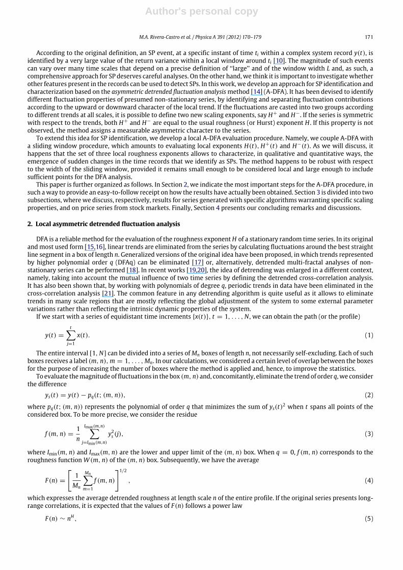
In Fig. 1, we illustrate the implementation of the local A-DFA1 to the Weierstrass function W0.5(t) with 2500 points. Asstated above, the dependence of all three functions F(n), F(n)± on n shows a very precise linear dependence in the double-logarithmic plot with slope 0.5when thewhole data sample is considered (not shown). Fig. 1a and b showhowH0(t),H+(t),and H−(t) depend on t when the analysis and evaluation is restricted to a sliding window of width L = 100. It is possible tonote small fluctuations on the value ofH(t) aroundH = 0.5 relatedwith amuch smaller used statistics, but such fluctuationsbecome smaller when the width of the sliding windows increases. We further observe that, for the samewindowwidth, thefluctuations on the values of H+(t) and H−(t) are undoubtedly larger than those of H(t), and that they are overwhelminglyout of phase, i.e., when H+(t) > H(t) it is more likely that H−(t) < H(t) and vice-versa. In Fig. 1c, we draw the differenceH+(t) − H−(t) to show more clearly the out of phase feature.

Author's personal copy

M.A. Rivera-Castro et al. / Physica A 391 (2012) 170–179 173

a

b

c

Fig. 1. Time dependency of a well known profile W0.5(t) (black) together with the corresponding local Hurst exponents H(t) (red–gray) (a). In panel (b),the asymmetric Hurst exponents H+(t) (black) and H−(t) (red–gray) and, in (c), the difference H+(t) − H−(t). (For interpretation of the references tocolour in this figure legend, the reader is referred to the web version of this article.)

It becomes more convenient to illustrate the dependence of the exponents as a function of L in the case of two isolatedpeaks in a flat profile, as shown in Fig. 2a. The results in Fig. 2b show clearly that the values of Hi depend on L. In Fig. 2c,we illustrate the behavior of H+(t) and H−(t). Note that, if the peak is antisymmetric with respect to t = 0, we obtainH+(t) = H−(−t). The superposition of an external peak to a random record leads also to very sharp changes in the valuesof H i(t) in the neighborhood of the peak, as shown in the second half of the profile in Fig. 2a–d. Special features for theisolated peak on the l.h.s include the following: the effect of L on the interval where H i(t) is non zero; a structured peakwith the presence of several satellites; the displacement of the maxima of H i(t) with respect to the peak maxima. The mostimportant feature for the superimposed peak on the r.h.s refers to an increase in the value ofH i(t) in the region that dependson the σ and on L.

Fig. 2 makes it evident that, for the single peak, the maximum value attained by H i(t) does not coincide with the peak.This can be easily understood when we consider the evaluation of H(t). Its maximum value corresponds to the instants of tsuch that the interval [t−L/2, t+L/2] covers one side (ascending or descending) of the peak. Tomake themaximumofH(t)coincide with themaximum of the peak it is necessary to shift the coordinate ofH(t) by L/2. To proceed in a symmetric way,we consider the combinationH(t−L/2)H(t+L/2) ≡ H(t), as shown in Fig. 2d (red line). Note that the so defined valueH(t)is the square of the geometrical average betweenH(t − L/2) andH(t + L/2). We have found out that such definition is moresuitable for localizing SPs as they reduce the production of satellite peaks that are produced by the arithmetic average. Thegraphs show a good coincidence in the location of the peaks, but it still depends strongly on L. In Fig. 2d, we also show (blackline) the difference between the shifted values H

±(t) ≡ H±(t − L/2)H±(t + L/2). Besides the agreement in the location of

the peaks, we can also observe an enhancement of the magnitude. This is caused by the fact that, when the peak reaches itslocal minimum, H

+also attains a local minimum and H

−a local maximum. On the contrary, when the peak reaches a local

maximum the value of H−reaches a local minimum and H

+a local maximum.

The shift in the value of the argument of H i(t) provides a good agreement with the extreme position in single peaksituations, but the situation of random series deserves a further discussion. The discussion above applies with somerestrictions. Let us observe that, since the series fluctuates randomly, local minima and maxima may occur in a variety ofways: embedded in a neutral trend patch, at the beginning or at the end of the persistent trend patch, and so on. Therefore,the combination of all these factors lead to the fact that, depending on L, many local extreme points do follow this rule, butsome fail to satisfy them. Another empirically observed interesting effect is that the behavior of H i(t) becomes similar tothat of H

i(t), as one can observe from the results in the r.h.s of Fig. 2c.

The effect of shifting the arguments of the exponents for the purpose of getting a good correspondence with the locationof the peaks becomes quite evident in the combinationsH

+(t)−H

−(t) and 2H(t)−H

+(t)−H

−(t), which can be regarded as

the subtraction and sum ofH±(t)−H(t). This is shown in Fig. 3a and b. There we show that local extreme ofW0.5 frequently

Author's personal copy

174 M.A. Rivera-Castro et al. / Physica A 391 (2012) 170–179

a

b

c

d

Fig. 2. Dependence of local H i(t) on the window size L for deterministic profiles: in panel (a), we consider a peak given by the derivative of a Gaussiancurve with variance σ = 15 (l.h.s), together with a Gaussian peak of variance σ = 12 superimposed on the same W0.5(t) profile (indicated by an arrowin the r.h.s). In (b), the usual H(t) with window widths L = 60 (black) and L = 100 (red–gray). For the sake of a clearer picture, in (c) we draw only thecurves for H+(t) (black) and H−(t) (red–gray) when L = 100. (For interpretation of the references to colour in this figure legend, the reader is referred tothe web version of this article.)

a

b

c

Fig. 3. Dependence of the shifted combinations H+(t) − H

−(t) (b) and 2H(t) − H

+(t) − H

−(t) (c) for the W0.5(t) profile (a). It is possible to notice a

quite nice agreement in SPs on (a) with the extreme values in (b) and (c). In (c), we included the extreme values ∆H obtained by the procedure describedin the text.

occur together with extreme of H+(t) − H

−(t). Note that, depending on H

+(t) being larger or smaller than H

−(t) and the

relation about the minimum or maximum values of the record with minimum or maximum values of H±(t), the magnitude

Author's personal copy

M.A. Rivera-Castro et al. / Physica A 391 (2012) 170–179 175

a

b

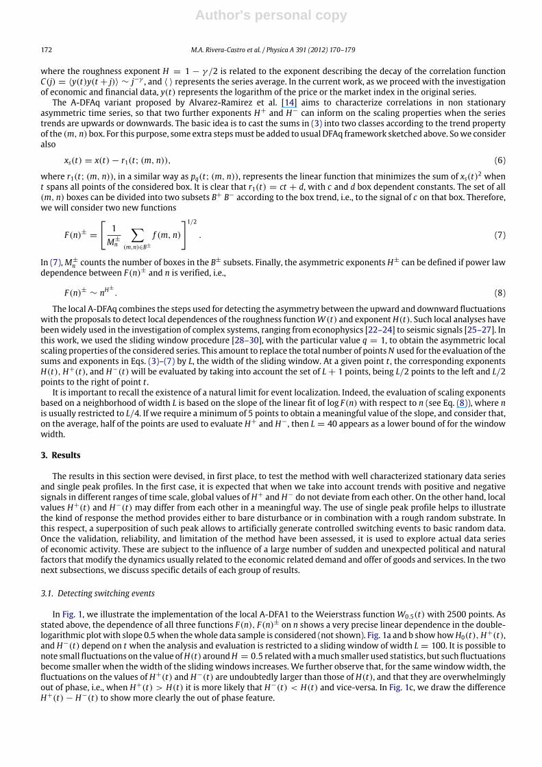
Fig. 4. WTI (a) and DJIA (b) time evolution with the indication of the periods that are subject to a closer analysis in Figs. 6–8.

of extreme values ofH+(t)−H

−(t) are enhanced in the following conditions: (a) the extreme is amaximumandH

+> H

−;

(b) the extreme is a minimum and H+

< H−. On the other hand, the magnitude is depleted in opposite conditions: (a) the

extreme is a maximum and H+

< H−; (b) the extreme is a minimum and H

+> H

−.

The smoother sign provided by 2H − H+

− H−offer a further possibility to identify SPs. Fig. 3c shows that these two

desired features are present herein. Nevertheless, themagnitudes ofmaxima andminima are subject to the same restrictionspointed out for the curve H

+− H

−.

These features bring some difficulties if one wants to associate the magnitude of the extreme values to that of theswitching points. So let us discuss the method we developed to minimize this asymmetric effect. First, we use a procedureto locate SPs in the two series H

+− H

−and 2H − H

+− H

−, although it can be used in any time series y(t) and extract

local maxima and minima. The output is a new series z(t). We may choose the width ℓ of the interval of contiguous pointsused to decide whether a point (t, y(t)) is an extreme or not. It is a local maximum only if y(t − j) < y(t) > y(t + j) for0 < j ≤ ℓ If y(t) is not an extreme, what is observed for the large majority of values of t , we set z(t) = 0. If it is an extreme,we select this specific value of t and identify it as Ti. Then we set z(i) = y(Ti −1)−2y(Ti)+ y(Ti +1). This procedure allowsthe identification of extreme based only on a local analysis, and that the magnitude of z(i) takes into account the values ofthree contiguous extreme values of y(T ). This way the asymmetry in themagnitude of H

+−H

−and 2H −H

+−H

−will be

reduced. The spikes in Fig. 3c identify the values z(ti) → ∆H detected by the described procedure. Note that larger valuesof ℓ imply that detected SPs follow after larger patches of coherent ascending and descending trends detected by the valuesof exponents H i, and that the value of z(i) may be also affected by the value of ℓ.

This procedure also opens the possibility for gauging the strength of an SP by the corresponding z(ti) value. Indeed it isquite natural to use the condition |z(ti)| > zc , where zc takes into account the typical order of magnitude of the series z(ti),to decide whether a point y(ti) is an SP or not. This criterion will be used in the next subsection with the analysis of actualeconomic series.

3.2. Switching events in actual series

The methods described in the former subsection have been applied to two well known economic series: Dow JonesIndustrial Average (DJIA) andWest Texas Intermediate (WTI), which reflects the oil price fluctuations, being more sensitiveto global political events that influence the market behavior of this commodity. In Fig. 4, we illustrate the time dependenceof both series: DJIA from 23/05/1980 to 25/08/2008, and WTI from 02/01/1986 to 14/12/2010. The complete series werefirst used for the purpose of investigating the frequency and magnitude of SP events with respect to the values of ℓ andL. However, since they are quite large, we concentrated our qualitative analyses to three distinct periods: (i) from 1985 to1988, encompassing the October 1987 crash (Oct87, with DJIA); (ii) a period corresponding to the relative stable oil priceyears 1994–1997 after the Gulf war (94–97, withWTI); (iii) and the sustained oil price increasing period that started in 2006until 2009, containing the 2008 world economic crash (with WTI).

Author's personal copy

176 M.A. Rivera-Castro et al. / Physica A 391 (2012) 170–179

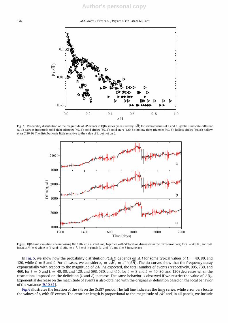
Fig. 5. Probability distribution of the magnitude of SP events in DJIA series (measured by ∆H) for several values of Ł and ℓ. Symbols indicate different(L, ℓ) pairs as indicated: solid right triangles (40, 5); solid circles (80, 5); solid stars (120, 5); hollow right triangles (40, 8); hollow circles (80, 8); hollowstars (120, 9). The distribution is little sensitive to the value of ℓ, but not on L.

a

b

c

Fig. 6. DJIA time evolution encompassing the 1987 crisis (solid line) together with SP location discussed in the text (error bars) for L = 40, 80, and 120.In (a), ∆Hc = 0 while in (b) and (c) ∆Hc = e−1 . ℓ = 8 in panels (a) and (b), and ℓ = 5 in panel (c).

In Fig. 5, we show how the probability distribution P(∆H) depends on ∆H for some typical values of L = 40, 80, and120, while ℓ = 5 and 9. For all cases, we consider zc = ∆Hc = e−1

⟨∆H⟩. The six curves show that the frequency decayexponentially with respect to the magnitude of ∆H . As expected, the total number of events (respectively, 995, 739, and460, for ℓ = 5 and L = 40, 80, and 120, and 698, 580, and 415, for ℓ = 8 and L = 40, 80, and 120) decreases when therestrictions imposed on the definition (L and ℓ) increase. The same behavior is observed if we restrict the value of ∆Hc .Exponential decrease on the magnitude of events is also obtained with the original SP definition based on the local behaviorof the variance [9,10,31].

Fig. 6 illustrates the location of the SPs on the Oct87 period. The full line indicates the time series, while error bars locatethe values of ti with SP events. The error bar length is proportional to the magnitude of ∆H and, in all panels, we include

Author's personal copy

M.A. Rivera-Castro et al. / Physica A 391 (2012) 170–179 177

a

b

c

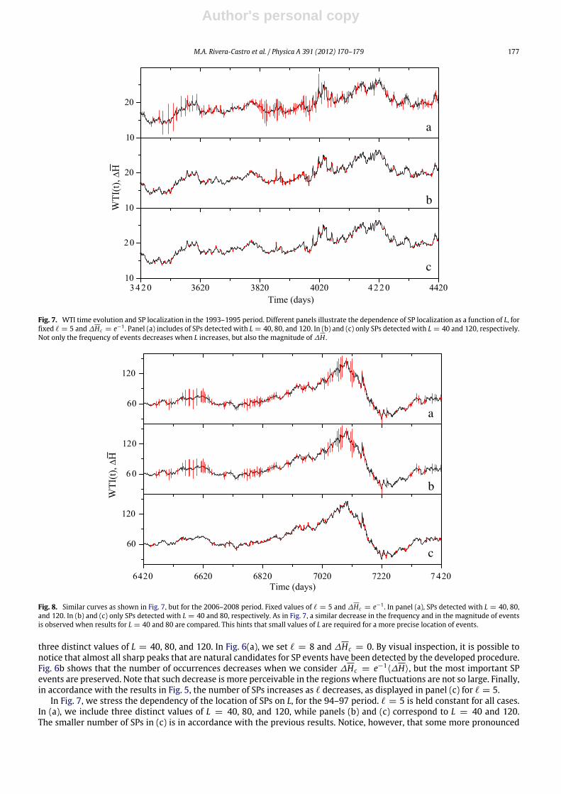
Fig. 7. WTI time evolution and SP localization in the 1993–1995 period. Different panels illustrate the dependence of SP localization as a function of L, forfixed ℓ = 5 and ∆Hc = e−1 . Panel (a) includes of SPs detected with L = 40, 80, and 120. In (b) and (c) only SPs detected with L = 40 and 120, respectively.Not only the frequency of events decreases when L increases, but also the magnitude of ∆H .

a

b

c

Fig. 8. Similar curves as shown in Fig. 7, but for the 2006–2008 period. Fixed values of ℓ = 5 and ∆Hc = e−1 . In panel (a), SPs detected with L = 40, 80,and 120. In (b) and (c) only SPs detected with L = 40 and 80, respectively. As in Fig. 7, a similar decrease in the frequency and in the magnitude of eventsis observed when results for L = 40 and 80 are compared. This hints that small values of L are required for a more precise location of events.

three distinct values of L = 40, 80, and 120. In Fig. 6(a), we set ℓ = 8 and ∆Hc = 0. By visual inspection, it is possible tonotice that almost all sharp peaks that are natural candidates for SP events have been detected by the developed procedure.Fig. 6b shows that the number of occurrences decreases when we consider ∆Hc = e−1

⟨∆H⟩, but the most important SPevents are preserved. Note that such decrease is more perceivable in the regions where fluctuations are not so large. Finally,in accordance with the results in Fig. 5, the number of SPs increases as ℓ decreases, as displayed in panel (c) for ℓ = 5.

In Fig. 7, we stress the dependency of the location of SPs on L, for the 94–97 period. ℓ = 5 is held constant for all cases.In (a), we include three distinct values of L = 40, 80, and 120, while panels (b) and (c) correspond to L = 40 and 120.The smaller number of SPs in (c) is in accordance with the previous results. Notice, however, that some more pronounced

Author's personal copy

178 M.A. Rivera-Castro et al. / Physica A 391 (2012) 170–179

extreme SPs that have been not detected by L = 40 scanning have been included when the window is wider. A comparisonwith the results in Fig. 6 shows that the variation in the magnitude of the error bars is smaller, which can be explained bythe absence of huge fluctuations in the time series in the considered interval.

Finally, we consider in Fig. 8 amixed period characterized by a long and constant upward trend in the oil price that endedwith the 2008 world crisis. Here again the method captures the majority of local fluctuations in both phases. Fixing ℓ = 5we show, in (a), results for the three window widths L = 40, 80, and 120, while in (b) and (c) we restrict to the smaller andintermediate values L = 40 and 80.

4. Conclusions

For the purpose of investigating SP occurrence in financial series, we adapted the concept of A-DFA to obtain local valuesH±(t) that provide information on the upward and downward trends. The very fact that H± distinguish distinct scalingbehavior in periods with different trends suggested us to explore the potentiality of this methodology. Despite the factthat such measures identify basic changes in the series behavior, the analysis of isolated peaks suggested us to work withthe product of shifted values H±(t ± L/2). Indeed, the measures H±(t) were able to identify SPs also in deterministic andactual series. The framework is sufficiently tunable, by a small number of parameters related to the widths L and ℓ, andevent relative magnitude∆Hc , so that it is possible to choose two independent length scales under which the system can beanalyzed. The number and magnitude of detected SPs are related by the preselected values of the quoted three parameters,so that the more relevant events can be filtered accordingly.

Since the proposed method is more elaborated than just looking at the local neighborhood of the original series, wewould like to stress that, for practical purposes, this flexibility and the new information it is able to provide seems to justifyour approach. Let us also note that our analyses do not require to introduce time re-normalization between two extremevalues, as used in Ref. [10,31]. Finally, we point out that the results of the developedmethod can be still more relevant in theanalysis of data sets where the intrinsic persistent behavior of upward and downward patches is more distinct than thoseprovided here. Although it is well known that the crashes usually proceed in much shorter scale building upward times, theobtained average values of H±(t) do not differ that much from each other.

Acknowledgments

This work was partially supported by the following Brazilian funding agencies: CAPES, FAPESB (through the PRONEXprogram), and CNPq (individual grants and the INCTI-SC program).

References

[1] P.J.N.F. Johnson, P.M. Hui, Financial Market Complexity: What Physics Can Tell Us About Market Behaviour, Oxford University Press, Oxford, 2003.[2] F. Schweitzer, G. Fagiolo, D. Sornette, F. Vega-Redondo, A. Vespignani, D.R. White, Economic networks: the new challenges, Science 326 (2009)

422–425.[3] F. Schweitzer, G. Fagiolo, D. Sornette, F. Vega-Redondo, D.R. White, Economic networks: what do we know and what do we need to know? Advances

in Complex Systems 12 (2009) 407–422.[4] D. Sornette, A. Johansen, Large financial crashes, Physica A 245 (1997) 411–422.[5] D. Sornette, Why Stock Markets Crash: Critical Events in Complex Financial Systems, Princeton University Press, Princeton, 2003.[6] R.N. Mantegna, H.E. Stanley, Introduction to Econophysics: Correlations and Complexity in Finance, Cambridge University Press, Cambridge, 2007.[7] F.D. Foster, S. Viswanathan, Variations in trading volume, return volatility, and trading costs – evidence on recent price formation models, Journal of

Finance 48 (1993) 187–211.[8] L.H. Ederington, J.H. Lee, How markets process information – news releases and volatility, Journal of Finance 48 (1993) 1161–1191.[9] T. Preis, H.E. Stanley, How to characterize trend switching processes in financial markets, APCTP Bulletin 23–24 (2009) 18–23.

[10] T. Preis, H.E. Stanley, Switching phenomena in a system with no switches, Journal of Statistical Physics 138 (2010) 431–446.[11] T. Preis, H.E. Stanley, Econophysics approaches to large-scale business data and financial crisis, in: Ch. Trend Switching Process in Financial Markets,

Springer, 2010, pp. 3–26.[12] T. Preis, H.E. Stanley, Bubble trouble, Physics World 24 (2011) 29–32.[13] D. Sornette, A. Johansen, J.P. Bouchaud, Stock market crashes, precursors and replicas, Journal of Physique I 6 (1996) 167–175.[14] J. Alvarez-Ramirez, E. Rodriguez, J.C. Echeverria, A dfa approach for assessing asymmetric correlations, Physica A 388 (2009) 2263–2270.[15] J.G. Moreira, J.K.L. DaSilva, S.O. Kamphorst, On the fractal dimension of self-affine profiles, Journal of Physics A 27 (1994) 8079–8089.[16] C.K. Peng, S.V. Buldyrev, S. Havlin, M. Simons, H.E. Stanley, A.L. Goldberger, Mozaic organization of dna nucleotides, Physical Review E 49 (1994)

1685–1689.[17] J.W. Kantelhardt, E. Koscielny-Bunde, H.H. Rego, S. Havlin, A. Bunde, Detecting long-range correlations with detrended fluctuation analysis, Physica A

295 (2001) 441–454.[18] J.W. Kantelhardt, S.A. Zschiegner, E.K.-B.E , S. Havlin, A. Bunde, H.E. Stanley, Multifractal detrended fluctuation analysis of nonstationary time series,

Physica A 316 (2002) 87–114.[19] B. Podobnik, H.E. Stanley, Detrended cross-correlation analysis: a new method for analyzing two non-stationary time series, Physical Review Letters

100 (2008) 084102.[20] B. Podobnik, D. Horvatic, A.M. Petersen, H.E. Stanley, Cross-correlations between volume change and price change, Proceedings of the National

Academy of Sciences of USA 106 (2009) 22079–22084.[21] D. Horvatic, H.E. Stanley, B. Podobnik, Detrended cross-correlation analysis for non-stationary time series with periodic trends, Europhysics Letters

94 (2011) 18007.[22] T. Lux, Long-term stochastic dependence in financial prices: evidence from the german stock market, Applied Economic Letters 3 (1996) 701–706.[23] T. DiMatteo, T. Aste, M.M. Dacorigna, Long-term memories of developed and emerging markets: using the scaling analysis to characterize their stage

of development, Journal of Banking and Finance 29 (2005) 827–851.[24] D.O. Cajueiro, B.M. Tabak, Testing for long-range dependence in world stock markets, Chaos, Solitons and Fractals 37 (2008) 918–927.

Author's personal copy

M.A. Rivera-Castro et al. / Physica A 391 (2012) 170–179 179

[25] R.F.S. Andrade, O. Oliveira, A.L. Cardoso, L.S. Lucena, F.E.A. Leite, M.J. Porsani, R.C. Maciel, Exploring self-affine properties in seismograms,Computational Geosciences 13 (2009) 155–163.

[26] F.J. Herrmann, Seismic facies characterization by scale analysis, Geophysics Research Letters 28 (2001) 3871.[27] F.J. Herrmann, Seismic deconvolution by atomic decomposition: a parametric approach with sparseness constraints, International Computational

Engineering 12 (2005) 69.[28] D.O. Cajueiro, B.M. Tabak, The hurst exponent over time: testing the assertion that emerging markets are becoming more efficient, Physica A 336

(2004) 521–537.[29] D.O. Cajueiro, B.M. Tabak, Ranking efficiency for emerging markets, Chaos, Solitons and Fractals 22 (2004) 349–352.[30] K.P. Lim, R. Brooks, The evolution of stock market efficiency over time: a survey of the empirical literature, Journal of Economic Surveys 25 (2011)

69–108.[31] T. Preis, J.J. Schneider, H.E. Stanley, Switching processes in financial markets, Proceedings of the National Academy of Sciences of USA 108 (2011)

774–7678.