Effect of turbulent Prandtl number in the convective turbulent ...
Upload
khangminh22Category
view
0download
0
Technische Universitat MunchenInstitut fur Energietechnik
Lehrstuhl fur Thermodynamik
Modeling Turbulent Combustion and COEmissions in Partially-Premixed Conditions
Considering Flame Stretch and Heat Loss
Noah Eugen Klarmann
Vollstandiger Abdruck der von der Fakultat fur Maschinenwesen derTechnischen Universitat Munchen zur Erlangung des akademischenGrades eines
DOKTOR – INGENIEURS
genehmigten Dissertation.
Vorsitzender:
Prof. Carlo L. Bottasso, Ph.D.
Prufer der Dissertation:
1. Prof. Dr.-Ing. Thomas Sattelmayer2. Prof. Antonio Andreini, Ph.D.
University of Florence, Italy
Die Dissertation wurde am 06.03.2019 bei der Technischen Universitat Muncheneingereicht und durch die Fakultat fur Maschinenwesen am 05.06.2019 angenommen.

Vorwort
Die vorliegende Arbeit entstand wahrend meiner Tatigkeit am Lehrstuhlfur Thermodynamik der Technischen Universitat Munchen. Sie wurdevom Bundesministerium fur Wirtschaft und Energie (BMWi) sowie vonGeneral Electric im Rahmen des deutschen Forschungsverbundes AGTurbo gefordert.
Meinem Doktorvater Herrn Prof. Dr.-Ing. Thomas Sattelmayer bin ich zugroßem Dank fur die wissenschaftliche Betreuung dieser Arbeit verpflich-tet. Die Zusammenarbeit mit ihm hat mich stets inspiriert und maßgeb-lich die Qualitat dieser Arbeit gepragt. Ich bedanke mich auch fur die mirgestatteten Freiraume, in denen ich mich wahrend der Promotion weiter-entwickeln konnte.
Herrn Prof. Dr. Antonio Andreini danke ich fur die Ubernahme des Ko-referates und Herrn Prof. Dr. Carlo Botasso fur den Prufungsvorsitz.
Auch danke ich Herrn Dr. sc. Benjamin Zoller, welcher dieses Projekt sei-tens der Industrie betreute. Die fachlichen Diskussionen mit ihm habensehr zum Gelingen dieser Arbeit beigetragen.
Ich danke allen Studenten, die mich wahrend der Promotion begleitet ha-ben. Besonders hervorheben mochte ich dabei Christoph Wieland, dermich uber einen langen Zeitraum sowohl in der Numerik als auch beiden Experimenten tatkraftig unterstutzte.
Ich mochte mich bei allen ehemaligen Kollegen fur die tolle Atmosphaream Lehrstuhl bedanken. Hierbei mochte ich Frau Helga Bassett und FrauSigrid Schulz-Reichwald hervorheben, die mich bei samtlichen organi-satorischen Angelegenheiten geduldig unterstutzten. Weiterhin bedankeich mich bei den Werkstatten fur die Fertigung des Prufstandes sowie al-len Kollegen, die mir wahrend der experimentellen Phase mit ihrer Fach-kenntnis zur Seite standen: Nicolai Stadlmair, Georg Fink, Stephan Lellekund Michael Betz.
Aus manchen Mitstreitern wurden wertvolle Freunde: Tobias Hummel,Frederik Berger, Ehsan Arabian, Michael Hertweck, Nicolai Stadlmairund Georg Fink. Vielen Dank fur die zahlreichen schonen Momente inden letzten Jahren. Ich hoffe wir bleiben noch lange in Kontakt.
iii
Liebe Jelena, Deine Unterstutzung in der finalen Phase war beispiellos.Du hast einen großen Beitrag an der erfolgreichen Fertigstellung dieserArbeit und dafur danke ich Dir von ganzem Herzen.
Liebe Familie, ich bin stolz, mit Euch ein so großartiges Umfeld zu ha-ben. Ihr habt mir uber all die Jahre Eure bedingungslose Unterstutzungzukommen lassen. Euch habe ich alles zu verdanken.
Munchen, im Juli 2019 Noah Klarmann
iv
Abstract
This study investigates combustion and CO emissions in cold conditionsthat occur in gas turbines operating at part load conditions. Moreover,the key research findings are used to develop a modeling strategy thatis able to predict heat release and CO distributions. The models seek tosupport the development of new flexible designs and concepts for mod-ern gas turbines that meet the requirements of the imminent new energyage. Combustion is described on the basis of flamelet generated man-ifolds. Important effects like flame stretch and heat loss are efficientlyconsidered by a novel approach. Validation is performed by comparingthe numerically predicted heat release with experimental OH∗. Further-more, a new CO methodology is proposed. CO is derived from flameletswithin the turbulent flame brush. As the flamelet theory is not able to de-scribe the burnout chemistry downstream of the turbulent flame brush,a model is introduced that predicts the transition from the theory of in-finitely thin reaction zones to kinetically limited burnouts. Experimentshave been conducted in which spatially resolved CO is obtained in or-der to validate the proposed methodology. Moreover, the validation intwo different multi-burner cases is presented to demonstrate the model’scapability of predicting CO in various fuel-staging scenarios. In addi-tion, the CO modeling strategy is applied to a novel combustor conceptto show basic mechanisms that are relevant in the context of this work.
v


Kurzfassung
Diese Arbeit untersucht den Verbrennungsvorgang und die damitverbundenen CO-Emissionen in Gasturbinenbrennkammern bei Teil-last. In diesem Zusammenhang wird eine neue Modellierungsstra-tegie prasentiert, mit der sich die raumlichen Verteilungen vonWarmefreisetzung und CO vorhersagen lassen. Diese Modelle konnenfur die Entwicklung moderner Brennkammern und Betriebskonzeptefur Gasturbinen eingesetzt werden, die den Anforderungen des be-vorstehenden neuen Energiezeitalters entsprechen. Der Verbrennungs-vorgang ist auf Basis von eindimensionalen Flammenrechnungen mitdetaillierter Chemie unter Berucksichtigung von Flammenstreckungund Warmeverlusten modelliert. Weiterhin erfolgt die Validierung desWarmefreisetzungsmodells mit experimentellen OH∗-Verteilungen. DasVerbrennungsmodell kann zudem die CO-Verteilung innerhalb der tur-bulenten Flammenburste beschreiben. Da die eindimensionalen Flam-men stromab der Warmefreisetzungszone an Gultigkeit verlieren, wirdein neues Vorgehen fur die Beschreibung der chemischen Quellterme imCO-Ausbrand vorgestellt. Atmospharische Experimente wurden durch-gefuhrt, um lokal aufgelostes CO zu messen. Neben der Validierung vonglobalen Emissionen lassen sich so auch die einzelnen Untermodelle aufGultigkeit uberprufen. Daruber hinaus wird die Validierung von glo-balem CO in zwei verschiedenen Mehrbrenneranordnungen vorgestellt.Diese Studie demonstriert die Fahigkeit der Modelle CO in verschiedenenSzenarien der Brennstoffstufung vorherzusagen. Am Ende dieser Arbeitwerden die Modelle auf ein neuartiges Brennerkonzept angewandt.
vii


Contents
Contents
1. Introduction 1
1.1. Load Flexible Gas Turbines . . . . . . . . . . . . . . . . . . . . . . . 31.2. Goals of this Work and Previous Research . . . . . . . . . . . . . 71.3. Thesis Structure . . . . . . . . . . . . . . . . . . . . . . . . . . . . . . . 10
2. Fundamentals of Turbulent Combustion 13
2.1. Governing Equations for Reactive Flows . . . . . . . . . . . . . . 132.2. Modeling Turbulence . . . . . . . . . . . . . . . . . . . . . . . . . . . 182.3. Modeling Combustion . . . . . . . . . . . . . . . . . . . . . . . . . . 24
3. Modeling Combustion 39
3.1. Flamelet Generated Manifolds . . . . . . . . . . . . . . . . . . . . . 393.2. Modeling Flame Stretch and Heat Loss . . . . . . . . . . . . . . . 423.3. Application and Validation . . . . . . . . . . . . . . . . . . . . . . . 543.4. Model Comparison . . . . . . . . . . . . . . . . . . . . . . . . . . . . . 63
4. Modeling CO 67
4.1. Separating Time Scales . . . . . . . . . . . . . . . . . . . . . . . . . . 684.2. Modeling In-Flame CO . . . . . . . . . . . . . . . . . . . . . . . . . . 704.3. Modeling Post-Flame CO . . . . . . . . . . . . . . . . . . . . . . . . 734.4. Modeling the Transition to Post-Flame . . . . . . . . . . . . . . . 794.5. Modeling Lean Quenching . . . . . . . . . . . . . . . . . . . . . . . 804.6. Application and Validation . . . . . . . . . . . . . . . . . . . . . . . 83
5. Summary 109
A. Software Implementation 113
B. Additional Reaction Analysis 119
Bibliography 122
ix

List of Figures
List of Figures
1.1. Temperature dependent emissions of a premixed flame(adapted from Steinbach et al. [16]). . . . . . . . . . . . . . 4
1.2. Sketch of a piloted swirl burner (inspired by Guyot et al.[17]). . . . . . . . . . . . . . . . . . . . . . . . . . . . . . . . 6
1.3. Illustration of a gas turbine with silo combustion chamberon the left (inspired by Vorontsov et al. [22]) and an annularcombustion chamber on the right (inspired by Tripod et al.[23]). . . . . . . . . . . . . . . . . . . . . . . . . . . . . . . . 7
2.1. Turbulence energy spectrum (adapted from Peters [31] aswell as from Poinsot and Veynante [28]). . . . . . . . . . . . 20
2.2. Spatial profiles of selected quantities (freely-propagating atT = 512 K, p = 10 bar and φ = 0.75, calculated using GAL-WAY 1.3 [38] and CANTERA [34]). . . . . . . . . . . . . . . . 26
2.3. Visualization of the local orthonormal basis on the lefthand side and two radii describing curvature on the righthand side. . . . . . . . . . . . . . . . . . . . . . . . . . . . . 28
2.4. Temperature in a well-stirred reactor as a function ofDamkohler number (adapted from Peters [31]). . . . . . . . 30
2.5. Classification of turbulence-chemistry interaction in theBorghi diagram (adapted from Peters [31] as well asPoinsot and Veynante [28]). . . . . . . . . . . . . . . . . . . 31
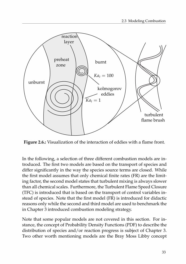
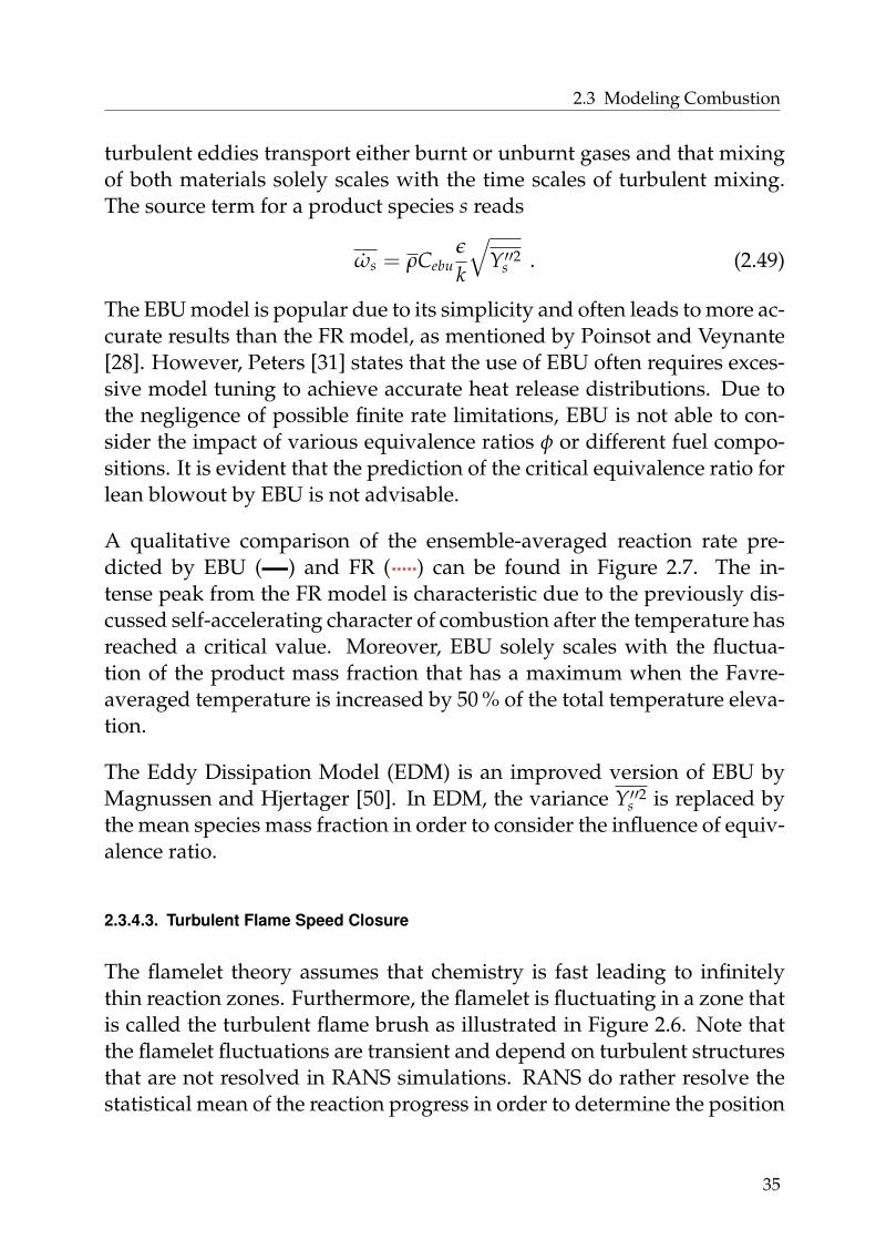
2.6. Visualization of the interaction of eddies with a flame front. 332.7. Demonstration of typical reaction rate profiles by FR and
EBU (adapted from Poinsot and Veynante [28]). . . . . . . 362.8. Visualization of the turbulent flame velocity (adapted from
Peters [31]). . . . . . . . . . . . . . . . . . . . . . . . . . . . 37
3.1. Simplified overview of the classical FGM. . . . . . . . . . . 41
xi

List of Figures
3.2. Justifying the flamelet theory for Marosky’s [58] validationcase as well as for gas turbines (Borghi diagram adaptedfrom Peters [31] and from Poinsot and Veynante [28]). . . . 43
3.3. Illustration of a premixed counterflow flame. . . . . . . . . 443.4. Demonstration of the constant character of mκ,ψ. . . . . . . 473.5. Demonstration of the independence of mκ,ψ from equiva-
lence ratio φ and heat loss. . . . . . . . . . . . . . . . . . . . 473.6. Simplified overview of FGM that considers stretch and
heat loss. . . . . . . . . . . . . . . . . . . . . . . . . . . . . . 493.7. Illustration of Marosky’s [58] validation case. . . . . . . . . 543.8. Distributions of velocity (upper half) and mixture fraction
(lower half) of Marosky’s [58] validation case. . . . . . . . . 553.9. Distributions of flame stretch, mean strain, turbulent
strain, and curvature of Marosky’s [58] validation case.. . . 583.10. Distribution of heat loss ψ of Marosky’s [58] validation case. 593.11. Reference fuel consumption speed s0
c (upper half) and thenon-adiabatic, strained fuel consumption speed s∗c (lowerhalf) of Marosky’s [58] validation case. . . . . . . . . . . . . 60
3.12. Demonstration of the influence of flame stretch and heatloss on flame speed. The corresponding values are volume-averaged over a numerically predicted turbulent flamebrush of Marosky’s validation case (cf. Table 3.2 and 3.3). . 61
3.13. Comparison of numerically predicted heat release with ex-perimental OH∗ emissivity data of Marosky’s [58] valida-tion case. . . . . . . . . . . . . . . . . . . . . . . . . . . . . . 62
3.14. Qualitative comparison of different standard combustionmodels. . . . . . . . . . . . . . . . . . . . . . . . . . . . . . . 65
4.1. Illustration of the domain partitioning that identifies thezones of different CO modeling. . . . . . . . . . . . . . . . . 68
4.2. Flame stretch dependency of CO demonstrated at threepressure levels (premixed counterflow flamelets at φ = 0.5,and Tu = 573.15 K calculated using GRI 3.0 [37] and CAN-TERA [34]). . . . . . . . . . . . . . . . . . . . . . . . . . . . . 71
4.3. Demonstration of the constant character of the proportion-ality exponents mκ,CO and mψ,CO. . . . . . . . . . . . . . . . 72
xii
List of Figures
4.4. Four most relevant CO reactions in the late burnout (con-stant pressure reactor at φ = 0.3, calculated using GALWAY
1.3 [38] and CANTERA [34]). . . . . . . . . . . . . . . . . . . 744.5. CO burnout time scales for different strategies of consider-
ing OH (reprinted and adapted from Flagan and Seinfeld[85]). . . . . . . . . . . . . . . . . . . . . . . . . . . . . . . . 76
4.6. Illustration of the atmospheric single-burner test rig withindicated post-flame measurement locations. . . . . . . . . 77
4.7. Comparison of experimental with modeled source terms ofCO. . . . . . . . . . . . . . . . . . . . . . . . . . . . . . . . . 78
4.8. Temperature dependent burnout time and ratio of OH cre-ation to CO oxidation (constant pressure reactor at p =15 bar, calculated using GALWAY 1.3 [38] and CANTERA [34]). 80
4.9. Five most relevant OH reactions in the late burnout (con-stant pressure reactor at φ = 0.3, calculated using GALWAY
1.3 [38] and CANTERA [34]). . . . . . . . . . . . . . . . . . . 824.10. Simplified overview of the CO model. . . . . . . . . . . . . 844.11. Illustration of the atmospheric single-burner test rig. . . . . 864.12. Contour plots of velocity u (upper half) and mixture frac-
tion f (lower half) of the atmospheric single-burner test rig. 874.13. Contour plots of CO mole fraction XCO of the atmospheric
single-burner test rig. . . . . . . . . . . . . . . . . . . . . . . 904.14. Contour plots of the modeling zones of the atmospheric
single-burner test rig. . . . . . . . . . . . . . . . . . . . . . . 914.15. Temperature dependent CO emissions of the atmospheric
single-burner test rig, which is illustrated in Figure 4.11. . 924.16. Illustration of of the GT11N (inspired by Vorontsov et al.
[22]) with fuel staging concept of the atmospheric GT11Nmodel. . . . . . . . . . . . . . . . . . . . . . . . . . . . . . . 94
4.17. Temperature dependent CO emissions of the atmosphericGT11N model. . . . . . . . . . . . . . . . . . . . . . . . . . . 97
4.18. Contour plots of CO mole fractions XCO of three character-istic loads of the atmospheric GT11N model. . . . . . . . . 98
4.19. Burner layout of the high-pressure GT11N in field operation.1004.20. Temperature dependent CO emissions of the high-pressure
GT11N in field operation. . . . . . . . . . . . . . . . . . . . 1004.21. Contour plots of the high-pressure GT11N in field operation.101
xiii

List of Figures
4.22. Illustration of the novel combustor concept that is inspiredby Lammel et al. [90]). . . . . . . . . . . . . . . . . . . . . . 102
4.23. Comparison of jet with swirl flames at an adiabatic temper-ature of Tad = 1620 K of the novel combustor concept. . . . 105
4.24. Temperature dependent CO emissions of the novel com-bustor concept. . . . . . . . . . . . . . . . . . . . . . . . . . 105
4.25. Contour plots of CO mole fraction XCO showing the inter-action of jet flames with colder neighbors of the novel com-bustor concept. . . . . . . . . . . . . . . . . . . . . . . . . . 107
A.1. Overview of the software implementation. . . . . . . . . . 113A.2. The work is divided in multiple threads that can be calcu-
lated in parallel. . . . . . . . . . . . . . . . . . . . . . . . . . 115A.3. Graphical user interface of the Table Generator. . . . . . . . 116
B.1. Four most relevant CO reactions in the late burnout (con-stant pressure reactor at φ = 0.5, calculated using GALWAY
1.3 [38] and CANTERA [34]). . . . . . . . . . . . . . . . . . . 120B.2. Five most relevant OH reactions in the late burnout (con-
stant pressure reactor at φ = 0.5, calculated using GALWAY
1.3 [38] and CANTERA [34]). . . . . . . . . . . . . . . . . . . 121
xiv
List of Tables
List of Tables
2.1. A selection of kinetic mechanisms for the combustion ofhydrocarbons (titer is determined from a constant pressurereactor at T = 512 K, p = 10 bar and φ = 0.75, calculatedusing CANTERA [34]). . . . . . . . . . . . . . . . . . . . . . . 17
3.1. Overview of estimated scales that occur in gas turbines andin Marosky’s [58] validation case. . . . . . . . . . . . . . . . 43
3.2. Summary of the numerical setup for Marosky’s [58] test rig. 573.3. Strain and curvature averaged over the turbulent flame
brush. . . . . . . . . . . . . . . . . . . . . . . . . . . . . . . . 59
4.1. Summary of the numerical setup for the atmosphericsingle-burner test rig. . . . . . . . . . . . . . . . . . . . . . . 88
4.2. Summary of the numerical setup for the multi-burner cases. 964.3. Summary of the numerical setup for the novel combustor
concept. . . . . . . . . . . . . . . . . . . . . . . . . . . . . . . 103
xv


Nomenclature
Nomenclature
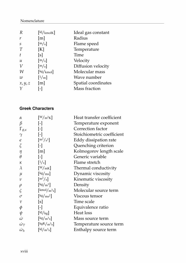
Latin Characters
A [m2] SurfaceA f req [(m3/kmol)
i−1/Ks] Pre-exponential factor
b [-] Stoichiometric mass ratio of oxidizer to fuelC [-] Number of atomsC [-] Generic model constantc [-] Reaction progresscp [kJ/kgK] Heat capacityD [m2/s] Diffusion coefficientd [m] DiameterE [m3/s2] Turbulent kinetic energy in wave number spaceEa [kJ/kmol] Activation energyF [m/s2] Forcef [-] Mixture fractionh [kJ/kg] Enthalpy (sum of sensible and chemical enthalpy)∆h f orm [kJ/kg] Enthalpy of formationk [m2/s2] Turbulent kinetic energykarr [(m3/kmol)
i−1/s] Rate constant
l [m] LengthM [-] Number of speciesm [kg] Massmκ,ψ [-] Proportionality exponentm [kg/s] Mass flow rateN [-] Number of speciesn [-] Surface orientation factorPk [kg/ms3] Source term for turbulent kinetic energyp [kg/ms2] Pressureq [kJ/m2s] Diffusive flux of enthalpyR [-] Number of reactions
xvii
Nomenclature
R [kJ/kmolK] Ideal gas constantr [m] Radiuss [m/s] Flame speedT [K] Temperaturet [s] Timeu [m/s] VelocityV [m/s] Diffusion velocityW [kg/kmol] Molecular massw [1/m] Wave numberx, y, z [m] Spatial coordinatesY [-] Mass fraction
Greek Characters
α [W/m2K] Heat transfer coefficientβ [-] Temperature exponentΓψ,κ [-] Correction factorγ [-] Stoichiometric coefficientε [m2/s3] Eddy dissipation rateζ [-] Quenching criterionη [m] Kolmogorov length scaleθ [-] Generic variableκ [1/s] Flame stretchλ [W/mK] Thermal conductivityµ [kg/ms] Dynamic viscosityν [m2/s] Kinematic viscosityρ [kg/m3] Densityς [kmol/m3s] Molecular source termσ [kg/ms2] Viscous tensorτ [s] Time scaleφ [-] Equivalence ratioψ [kJ/kg] Heat lossω [kg/m3s] Mass source termωT [kgK/m3s] Temperature source termωh [kJ/m3s] Enthalpy source term
xviii

Nomenclature
Superscripts
0 Reference conditions∗ Stretched and/or non-adiabaticˆ Normalized
Ensemble mean′ Fluctuations regarding ensemble mean˜ Favre mean′′ Fluctuations regarding Favre mean
Subscripts
∞ Ambient conditions0/1 Mixture fraction of zero/unity15 Normalized to 15% dioxygenad Adiabatican Annulusb Burntburner Burnerc Fuel consumptionch Chemicalcr Creationcrit Criticalcurv Curvatured Displacementdi f f Diffusiondry Does not contain watereddy Turbulent vortexeq Equilibriumf Flamef uel Fuelf it Curve fittedf or/rev Forward/reversegen Genericign Ignitionint Integral
xix

Nomenclature
iter Iterationl Laminarlbo Lean blowoutmax Maximummodel Modeledox Oxidationoxid Oxidizerpri/sec Primary/secondaryq Quenchedr Reactorsens Sensiblest Strainsto Stoichiometrict Turbulentt f b Turbulent flame brushth Thermaltrans Transitionu Unburntw Wrinklingwall Wall
Control Indices
i, j, k Spatial indicesr Reaction indexs, t Species indices
Functions
I [-] Intermittent Turbulence Net Flame StretchP [-] Probability Density Function
xx

Nomenclature
Dimensionless Numbers
Da Damkohler numberDat Turbulent Damkohler numberKat Turbulent Karlovitz numberRe Reynolds numberSct Turbulent Schmidt number
Abbreviation
CFD Computational Fluid DynamicsDNS Direct Numerical SimulationEBU Eddy Break UpEDM Eddy Dissipation ModelFGM Flamelet Generated ManifoldFR Finite RateILDM Intrinsic Low-Dimensional ManifoldsITNFS Intermittent Turbulence Net Flame StretchLES Large Eddy SimulationODE Ordinary Differential EquationsPDF Probability Density FunctionRANS Reynolds-Averaged Navier-StokesRMS Root Mean SquareTFC Turbulent Flame Speed Closure
Molecules
CH4 Carbon tetrahydride (methane)CO Carbon monoxideCO2 Carbon dioxideH Molecular hydrogenH2 DihydrogenH2O Dihydrogen monoxide (water)HO2 Dioxidanyl (hydroperoxyl)N2 DinitrogenN2O Dinitrogen monoxide (nitrous oxide)
xxi

Nomenclature
NOx Nitrogen oxidesO Molecular oxygenO2 DioxygenOH Oxidanyl (hydroxyl)
Miscellenous
〈 〉 [-] Surface averaging[ ] [kmol/m3] Molecular concentrationℵ [-] Placeholder for chemical symbolsδ [-] Kronecker delta
xxii
1 Introduction
Human interventions in natural processes have never been more far-reaching than today. The industrialization caused a 40 % increase in car-bon dioxide (CO2), leading to destructive consequences for the ecologicalbalance of the planet according to the INTERGOVERNMENTAL PANEL ON
CLIMATE CHANGE [1]. Concentrations of greenhouse gases such as CO2,methane (CH4), and nitrous oxide (N2O) have never been higher in thelast million years. The oceans absorbed about 30 % of the anthropogenicCO2 leading to an ongoing process of seawater acidification that has adrastic impact on marine organisms [1]. Furthermore, the greenhouse ef-fect causes the earth’s surface, atmosphere, and oceans to heat up. Conse-quently, each of the last three decades has been warmer than the previousone as well as warmer than all other decades since 1850 [1]. In addition,the last thirty years have been the hottest in the Northern Hemispherein at least 1400 years [1]. This rise in temperature leads to multiple sideeffects that have never been observed in the last millennium. Droughts,storms, and melting of the polar ice caps are just a few of the numerousnegative impacts of global warming.
The world’s energy demand is predicted to increase approximately byabout 30 % between today and 2040 according to the INTERNATIONAL
ENERGY AGENCY [2, 3] and BRITISH PETROLEUM [4]. A major societalchallenge of the future is to cover the increasing energy demand while tosimultaneously reduce greenhouse gases. For this purpose, internationalconventions have been imposed, notably the PARIS AGREEMENT [5] orthe KYOTO PROTOCOL [6]. Due to the global trend of electrification, 70-80 % of the primary energy increase is used for the production of power[2, 4]. It should be noted that energy demand is not only a function of theexponential population growth, but also correlates with the improvementin efficiency, which reduces the energy per human consumption rate. Theenergy mix for power generation is expected to change drastically in the
1
Introduction
near future. Conventional power sources are anticipated to lose relevancedue to a significant increase in renewables, but retain its major role in theoverall energy mix. Besides advantages for the environment, renewableswill also become the best economical choice for most countries. Thus, twothirds of the global investment for power plants is expected to be spent onrenewable power production [3]. Furthermore, renewables will accountfor 40 % of the total increase in primary energy sources [3, 4]. While theproportion of oil and coal is predicted to decline, the use of natural gas isanticipated to increase significantly by 45 % between today and 2040 [3].In order to meet the increased demand for natural gas, new explorationand production techniques need to be developed [2]. What causes naturalgas to gain importance in the next decades? There are numerous obviousreasons such as efficiency and environmental legislations like emissionlimits1. A further reason is that power production by gas turbines playsa key role in the process of implementing a large share of renewables. Es-pecially small- to mid-sized gas turbines are able to quickly change theirload as mentioned by Wiedermann [7]. Volatilities of renewable powerproduction cause fluctuations that need to be compensated in order toguarantee a stable public grid frequency. Besides the compensation bychanging the load in terms of secondary control, gas turbines also act asprimary control systems2. Due to these properties, gas turbines are theideal counterpart to renewables and are thus a sustainable technology asmentioned by Sinn [9]. In order to prepare gas turbines for the challengesof tomorrow, reduction of emissions, increase of flexibility, efficiency, andreliability is of high technical relevance and the subject of numerous re-search projects nowadays.
Germany has a key role in the new energy age as it aims to becomethe technology leader in renewable power production to combat climatechange. In addition, Germany has the highest capacity and largest marketfor natural gas in the EUROPEAN UNION and is the most important coun-try for the transit of natural gas according to BUNDESMINISTERIUM FUR
1 Note that natural gas usually has a better hydrogen to carbon ratio than other conventional fuels and ishence more efficient in terms of power per CO2 emissions.
2 Primary control: Automatic frequency response within a time range of 30 s. Note that primary controlis passively achieved as the rotor of a gas turbine is a rotating mass that is synchronized with the publicpower grid according to the UNION FOR THE CO-ORDINATION OF TRANSMISSION OF ELECTRICITY [8].Secondary control: Changing load within minutes [8]..
2
1.1 Load Flexible Gas Turbines
WIRTSCHAFT UND ENERGIE [10]. Further expansion of the natural gasinfrastructure in Germany is planned for the near future as mentioned byDIE FERNLEITUNGSBETREIBER [11]. For example, gas-based generationcapacities with an accumulated power output of 883 MW are currentlybeing built, which is a third of the total amount of new capacities accord-ing to the BUNDESNETZAGENTUR [12].
1.1. Load Flexible Gas Turbines
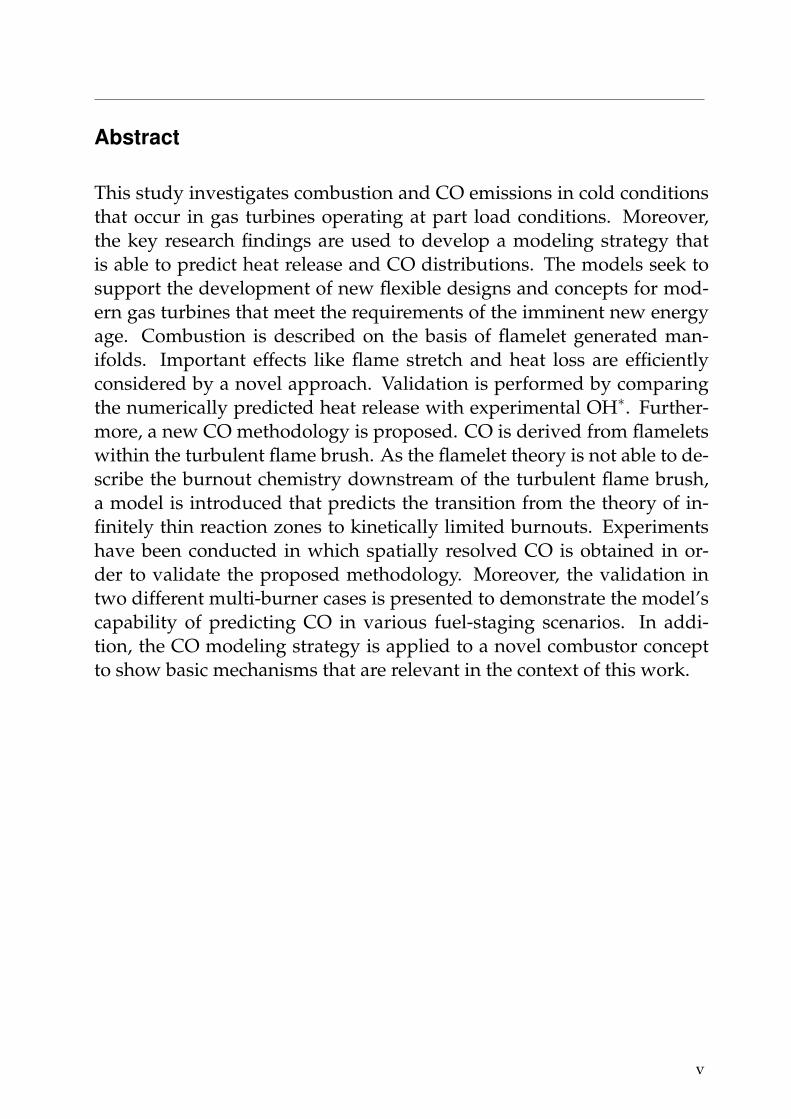
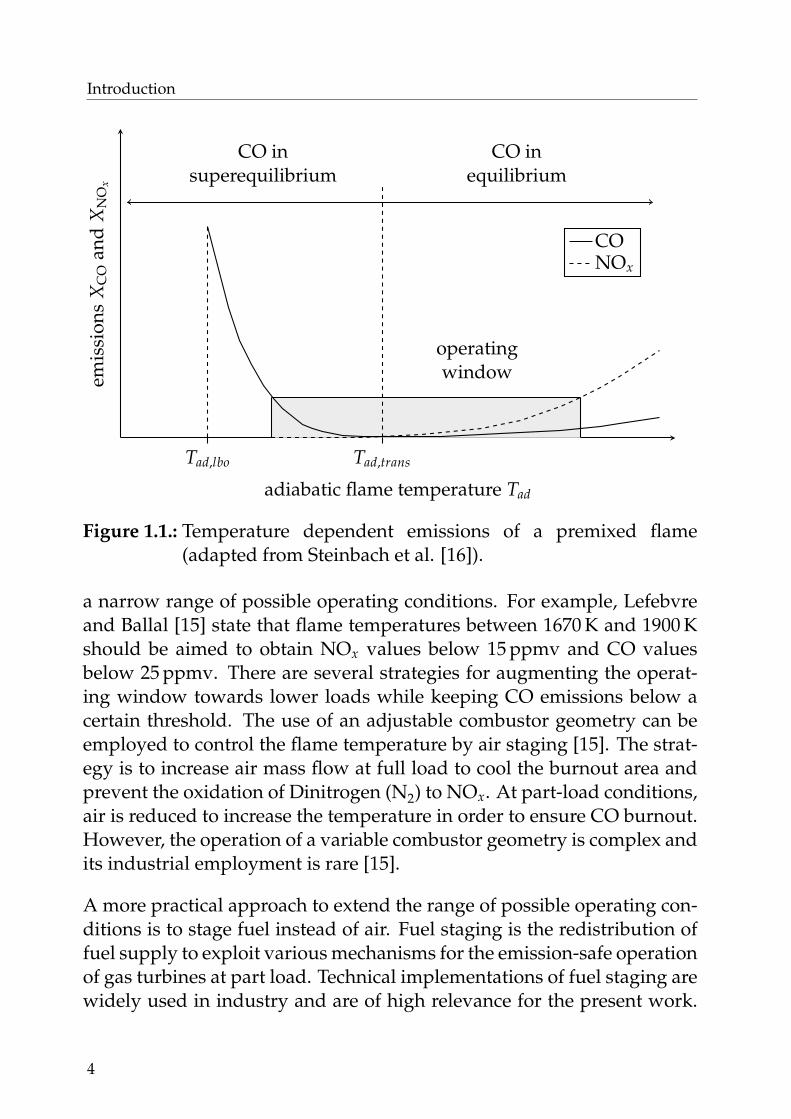
As discussed above, gas turbines may become increasingly crucial to com-pensate the emerging volatilities of renewables. In order to fulfill this role,modern gas turbines need to be able to perform fast load changes in alarge operating window. Load flexibility is hence an essential feature formeeting the requirements of tomorrow and is thus the subject of scientificengineering today. In general, load changes in gas turbines are achievedby adjusting the fuel supply as mentioned by Sattelmayer [13]. A simul-taneous reduction of the air mass flow can be accomplished to a certaindegree by means of adjusting the compressor’s guide vanes as discussedby Moning and Waltke [14]. Once the minimum air mass flow is reached,a further reduction in load leads to a decrease of the global fuel-to-air ra-tio and colder flames. Figure 1.1 qualitatively illustrates nitrogen oxide(NOx) and carbon monoxide (CO) emissions as a function of the adiabaticflame temperature Tad. NOx is mainly a function of temperature accord-ing to the Arrhenius law. The key difference between NOx and CO is thatthe latter is an intermediate species in the context of hydrocarbon-basedcombustion. CO usually reaches a maximum within the flame that is byorders of magnitude higher than the limits given by emission legislations.The burnout of CO is hence a crucial process to reduce CO emissions.Consequently, super-equilibrium CO may occur in cold conditions as thetemperature-sensitive burnout of CO cannot be completed. Under con-ditions that show sufficiently high temperatures, the burnout is fast andthe reactive flow quickly approaches equilibrium. Below a specific flametemperature Tad,trans, the equilibrium state can no longer be reached andCO emissions rise sharply. The lower limit of fuel reduction is given bythe lean blowout limit that occurs at an adiabatic temperature denoted asTad,lbo. The contrary trends in CO and NOx as functions of Tad may lead to
3
Introduction
Tad,lbo Tad,trans
operatingwindow
CO inequilibrium
CO insuperequilibrium
adiabatic flame temperature Tad
emis
sion
sX
CO
and
XN
Ox
CONOx
Figure 1.1.: Temperature dependent emissions of a premixed flame(adapted from Steinbach et al. [16]).
a narrow range of possible operating conditions. For example, Lefebvreand Ballal [15] state that flame temperatures between 1670 K and 1900 Kshould be aimed to obtain NOx values below 15 ppmv and CO valuesbelow 25 ppmv. There are several strategies for augmenting the operat-ing window towards lower loads while keeping CO emissions below acertain threshold. The use of an adjustable combustor geometry can beemployed to control the flame temperature by air staging [15]. The strat-egy is to increase air mass flow at full load to cool the burnout area andprevent the oxidation of Dinitrogen (N2) to NOx. At part-load conditions,air is reduced to increase the temperature in order to ensure CO burnout.However, the operation of a variable combustor geometry is complex andits industrial employment is rare [15].
A more practical approach to extend the range of possible operating con-ditions is to stage fuel instead of air. Fuel staging is the redistribution offuel supply to exploit various mechanisms for the emission-safe operationof gas turbines at part load. Technical implementations of fuel staging arewidely used in industry and are of high relevance for the present work.
4
1.1 Load Flexible Gas Turbines
Multiple strategies for fuel staging exist that can be characterized as fol-lows 3:
• Switching to non-premixed combustion: In this fuel staging con-cept, a switch from premixed to non-premixed combustion is con-ducted when load is decreased to a specific point. Non-premixedcombustion features diffusion flames that burn close to stoichiomet-ric conditions, which lead on the one hand to higher reactivity andadvantages in terms of burnout. On the other hand, the reactionzones of diffusion flames show higher flame temperatures and thusincreased NOx emissions. High NOx emissions can be avoided by us-ing solely a fraction of the fuel for the pilot . The remaining fuel is stillsupplied to the premixed burner leading to a reactive gas that can bebelow the lean blowout limit and still ignites after mixing with thehot gas from the pilot flame. This is possible as the minimum tem-perature for self-ignition chemistry is below the lean blowout tem-perature as stated by Sattelmayer [13].
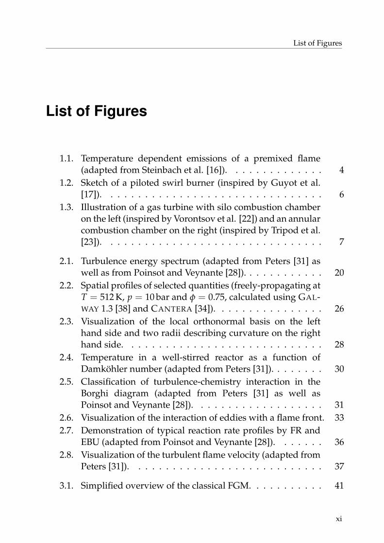
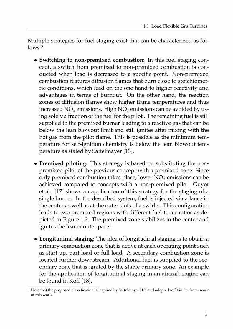
• Premixed piloting: This strategy is based on substituting the non-premixed pilot of the previous concept with a premixed zone. Sinceonly premixed combustion takes place, lower NOx emissions can beachieved compared to concepts with a non-premixed pilot. Guyotet al. [17] shows an application of this strategy for the staging of asingle burner. In the described system, fuel is injected via a lance inthe center as well as at the outer slots of a swirler. This configurationleads to two premixed regions with different fuel-to-air ratios as de-picted in Figure 1.2. The premixed zone stabilizes in the center andignites the leaner outer parts.
• Longitudinal staging: The idea of longitudinal staging is to obtain aprimary combustion zone that is active at each operating point suchas start up, part load or full load. A secondary combustion zone islocated further downstream. Additional fuel is supplied to the sec-ondary zone that is ignited by the stable primary zone. An examplefor the application of longitudinal staging in an aircraft engine canbe found in Koff [18].
3 Note that the proposed classification is inspired by Sattelmayer [13] and adapted to fit in the frameworkof this work.
5

Introduction
https://www.sciencedirect.com/science/article/pii/S0306261915004997
slots with fuel
injection
holespilot
fuel-to-air
induced
ratio
swirl
lance
injection
low
fuel-to-airratio
high
Figure 1.2.: Sketch of a piloted swirl burner (inspired by Guyot et al. [17]).
• Sequential combustion: Partial decompression during combustionhas thermodynamic advantages such as lower flame temperaturesand higher efficiencies. This principle is exploited in sequential com-bustion as fuel is supplied to multiple combustion chambers at dif-ferent levels of pressure. Technical implementations of this conceptcan be found by Dobbeling et al. [19], by Hiddemann et al. [20] or byGuthe et al. [21].
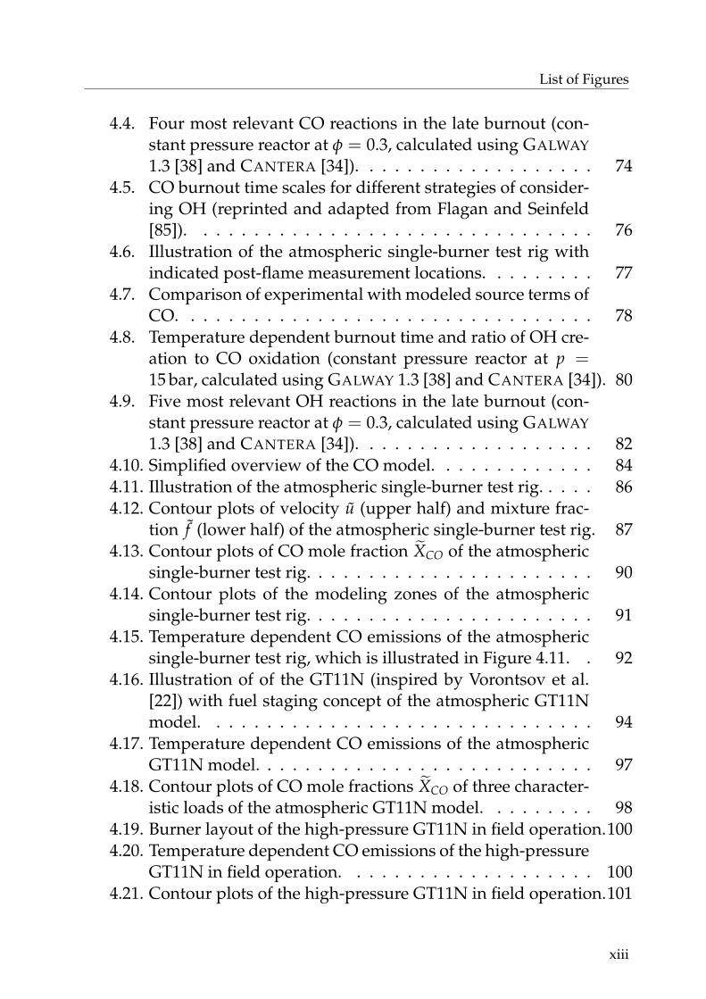
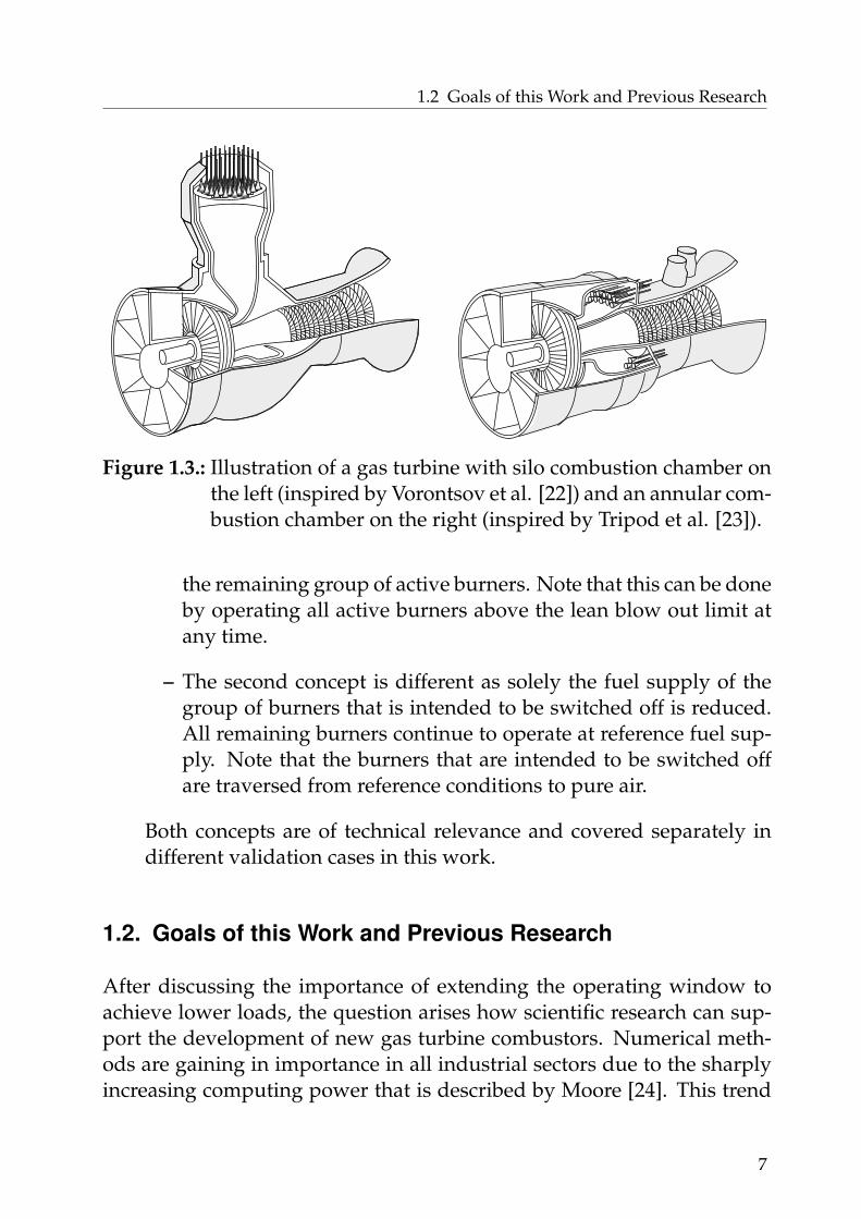
• Fuel staging in multi-burner systems: The previous fuel stagingconcepts do not take advantage of the fact that gas turbines usu-ally employ multiple burners. Examples for burner arrangements inmulti-burner systems are illustrated in Figure 1.3. There is on the onehand the option of implementing the aforementioned concepts foreach burner individually. On the other hand, multi-burner systemsopen up the possibility of exploiting the interaction between adja-cent burners to apply further fuel staging strategies. Multi-burnerfuel staging concepts usually have multiple stages. At each stage, apredefined group of burners is switched off. There are two differentparadigms in the way fuel is decreased before the switch-off eventsoccur:
– In the first concept, fuel supply of all active burners is evenly de-creased before a group of burners is switched off. By deactivatinga group of burners, the fuel surplus needs to be redistributed to
6
1.2 Goals of this Work and Previous Research
Figure 1.3.: Illustration of a gas turbine with silo combustion chamber onthe left (inspired by Vorontsov et al. [22]) and an annular com-bustion chamber on the right (inspired by Tripod et al. [23]).
the remaining group of active burners. Note that this can be doneby operating all active burners above the lean blow out limit atany time.
– The second concept is different as solely the fuel supply of thegroup of burners that is intended to be switched off is reduced.All remaining burners continue to operate at reference fuel sup-ply. Note that the burners that are intended to be switched offare traversed from reference conditions to pure air.
Both concepts are of technical relevance and covered separately indifferent validation cases in this work.
1.2. Goals of this Work and Previous Research
After discussing the importance of extending the operating window toachieve lower loads, the question arises how scientific research can sup-port the development of new gas turbine combustors. Numerical meth-ods are gaining in importance in all industrial sectors due to the sharplyincreasing computing power that is described by Moore [24]. This trend
7
Introduction
disrupts conventional development processes, as costly experiments canbe partially replaced by simulations. Note that this applies in particularto the development of complex systems such as gas turbine combustorsthat are operated at high-pressure conditions. Hence, interest in the nu-merically supported design of new combustors and operating concepts issteadily increasing as inefficient design-built-measurement cycles can beavoided.
The aim of this work is to develop a modeling strategy that is capable ofaccurately predicting combustion and the corresponding CO emissionsin gas turbines that operate at part-load conditions. Computational FluidDynamics (CFD) is well suited in order to achieve the specified goals.In CFD, governing equations are employed, which are able to describequantities continuously in space. Note that the consideration of local ef-fects is crucial for this work. For instances, the above introduced con-cepts of fuel staging are based on numerous local effects that cannot becovered by integral approaches. In general, CFD is able to describe flow,combustion and emissions in an exact4 way. However, the direct solu-tion is resource intense as vast grids are necessary to resolve all turbulentstructures. Thus, modeling is necessary to drastically reduce the com-putational effort. The models of the present work seek to support thedevelopment of new gas turbine combustion systems. In order to createan approach that is able to be applied in industry, different requirementshave to be met. All models should work under pressure conditions thatrange from atmospheric pressure5 to the full range of high-pressure con-ditions of modern gas turbines. The modeling strategy must be able tocover the situation of pilot operation where a stable reaction zone ignitesgases that are below the lean blowout limit. In addition, a possible imple-mentation of the proposed models in industrial processes requires highprecision6 at low computational costs.
4 It should be noted that the governing equations are actually derived with simplifications. However, thedirect solution of the governing equations is sufficiently accurate in a way that is relevant for technicalapplications.
5 The model validity at atmospheric conditions is necessary as validation data may be measured in atmo-spheric test rigs.
6 A precise model implies the ability to accurately predict physicochemical quantities without model tun-ing.
8

1.2 Goals of this Work and Previous Research
One may ask why existing, widely used combustion models are not ableto achieve the objectives of the present work. An often used simplifica-tion of standard combustion models is the assumption that a turbulentflame brush can be described by a set of laminar flamelets (referred toas the flamelet assumption). Flamelets are thin reaction zones that di-vide unburnt from burnt material. The oxidation of CO in flamelets isfast due to the availability of a stable radical pool and CO always reachesequilibrium in short length and time scales. In contrast to the flameletassumption, part-load combustion in gas turbines usually features super-equilibrium CO in the exhaust gas far behind the heat release zone. Aflamelet-based combustion model can only predict elevated CO emis-sions at the outlet when flamelets fluctuate through the whole combus-tion chamber. The occurrence of flamelets in the exhaust gas is not re-alistic as the flame usually anchors close to the burner exit. Neverthe-less, the prediction of CO using the popular Flamelet Generated Mani-fold (FGM) model can be found by Goldin et al. [25,26]. Here, tuning of asemi-empirical closure is necessary to achieve a reasonable prediction ofCO. The authors conclude that FGM drastically overestimates the sourceterms of CO oxidation. Another attempt to numerically predict CO us-ing CFD can be found by Wegner et al. [27]. In the described approach,CO is determined by an own transport equation. Within the turbulentflame brush, CO is initialized with its peak value at a predefined reactionprogress. The peak value of CO is determined by one-dimensional simu-lations based on detailed chemistry. The approach by Wegner et al. [27]has several simplifications that are not accurate as argued later.
Based on literature research and the industrial requirements specifiedabove, the following requirements for the CFD-based modeling approachare identified:
• Momentum: The technical relevance of this work requires to focuson efficient models. Hence, the proposed modeling strategy is basedon averaged equations that neglect all turbulent structures.
• Mass and Species: The combustion time scales are orders of mag-nitude smaller than the time scales of the late CO burnout. Thus,a divide and conquer approach is reasonable: Two different models
9
Introduction
are developed, covering combustion on the one hand and the lateCO burnout on the other hand. It is worth noting that the CO modeldepends on the combustion model but not vice versa.
– Combustion: The simulation of combustion in gas turbines atpart load requires an advanced modeling strategy. Combustionin cold conditions is demonstrated to be in particularly suscepti-ble for flame stretch and heat loss. Hence, a combustion model isproposed that takes both effects into account. Furthermore, thecombustion model is able to consider partially-premixed com-bustion in order to cover quenching effects due to secondary airor the effect of poor mixing quality.
– CO model: The aforementioned separation of time scales is cru-cial for the successful modeling of CO. Hence, CO is describedindependently from the combustion model. Within the turbulentflame brush, CO is modeled on the basis of flamelets. Down-stream of the turbulent flame brush, the burnout of CO is domi-nated by chemical time scales and is thus described by chemicalmodels.
• Energy: Heat loss may significantly effect both combustion and COespecially in cold conditions. This is why the temperature drop dueto non-adiabatic effects must be taken into account. For this reason,the proposed modeling strategy is able to consider heat loss.
1.3. Thesis Structure
In the following, the structure of the thesis is presented. Chapter 2 intro-duces the theoretical fundamentals that are relevant for this work. Chap-ter 3 shows the combustion model that covers important effects, whichare relevant for cold conditions. An application of the combustion modelto an atmospheric single-burner test rig is shown. Numerical results arecompared to experimental OH∗7 in order to qualitatively evaluate themodel’s performance. In addition, a comparison of the proposed mod-
7 OH∗ is an excited hydroxyl molecule that can be used to indicate heat release distributions.
10

1.3 Thesis Structure
eling strategy with standard, widely used combustion models is shown.Chapter 4 presents the CO model that consists of several submodels. Lo-cally resolved measurements of CO emissions are crucial for the valida-tion of the individual parts of the CO model. For this reason, experimentsto measure CO distributions within the combustion chamber have beenconducted. Validation of the CO model in various fuel-staging scenariosis shown in two different multi-burner cases. Furthermore, the modelsare applied to an advanced combustor design. This work is finalized withChapter 5 where the content of this work is recapitulated.
11

2 Fundamentals of TurbulentCombustion
This chapter introduces the fundamentals of turbulent, reactive flows thatare relevant for the present work. Section 2.1 presents a set of governingequations for reactive flows. In addition, the modeling of turbulence isaddressed in Section 2.2. The last Section 2.3 covers turbulent combustion.
2.1. Governing Equations for Reactive Flows
The decisive difference between the mathematical description of reactiveand non-reactive flows is that the conversion of species requires to viewthe gas as a mixture that may significantly change its composition overtime. This leads to three challenges in formulating governing equationsfor reactive flows as stated by Poinsot and Veynante [28]:
• Reactions are able to change the species composition of the fluid.This usually leads to a tremendous change of the thermodynamicproperties. Thus, all species must be tracked in order to evaluatequantities like temperature, density, and heat capacity.
• The source term of each species must be closed. Hence, knowledgeof the combustion chemistry is required.
• Multi-component diffusion of momentum, species, and energy is ofhigh complexity and requires modeling.
In the following, a brief introduction of the governing equations for non-isothermal, reactive flows is given. The continuous description of mo-mentum, mass, and energy forms the basis to numerically solve combus-tion problems. A more detailed view on this set of equations is given by
13

Fundamentals of Turbulent Combustion
Kuo [29], by Williams [30], and in a more compact form by Poinsot andVeynante [28] as well as by Peters [31].
2.1.1. Mass
As combustion is mass conservative, the classical form of the continuityequation can be used for the description of reactive flows:
∂ρ
∂t+
∂ρui
∂xi= 0 . (2.1)
This equation states that the local rate of mass change in a control volumeis solely caused by convective mass exchange with the environment.
2.1.2. Momentum
Momentum can be described by
∂ρuj
∂t+
∂ρuiuj
∂xi= − ∂p
∂xj+ ρ
N∑s=1
YsFs,j +∂σij
∂xi. (2.2)
The left hand side consists of the local rate of momentum change anda convective term. On the right hand side, momentum changes due topressure effects is described by the first term. Moreover, the second termspecifies the influence of volume forces Fs,j on momentum. Here, Fs,j actssolely on the fraction of mass that corresponds to species s. Thus, Fs,j mustbe multiplied by the species mass fraction Ys that reads
Ys =ms
m. (2.3)
In addition, the third term of Equation 2.2 tracks momentum changes dueto viscous dissipation in which σij is the viscous tensor:
σij = −23
µ∂uk
∂xkδij + µ
(∂ui
∂xj+
∂uj
∂xi
). (2.4)
Here, µ denotes the dynamic viscosity and δij the Kronecker delta. Notethat Equation 2.2 does not feature additional terms to consider charac-
14
2.1 Governing Equations for Reactive Flows
teristics from reactive flows. Nevertheless, combustion is implicitly cap-tured as viscosity and density change significantly.
In order to describe the coupling between velocity and pressure, two dif-ferent paradigms exist. In density-based approaches, the density field iscalculated by the continuity equation and pressure subsequently by theideal gas law. Pressure-based methods calculate pressure using algebraicmodels on the basis of the velocity field in a way that continuity is satis-fied. The CFD code that is used in this work employs a pressure-basedscheme by Patankar [32] called SIMPLE.
2.1.3. Species
As mentioned before, species must be tracked in order to derive the ther-modynamic state of the flow. The transport equation for species s reads
∂ρYs
∂t+
∂ρuiYs
∂xi= −∂ρVs,iYs
∂xi+ ωs . (2.5)
Species diffusion is described by the first term on the right hand sidein which Vs,i is the diffusion velocity of species s in i-th direction. Asdemonstrated by Williams [30], an analytical solution to multi-componentspecies diffusion exists. However, implementations of the proposed gov-erning equations usually employ diffusion models in order to keep thenumerical effort low. In this work, the one-dimensional flamelet sim-ulations model diffusion by employing a first-order approximation ofthe Chapman-Enskog theory by Chapman et al. [33]. Note that theChapman-Enskog theory considers multi-component diffusion instead ofusing mixture-averaged diffusion coefficients.
The second term on the right hand side of Equation 2.5 describes thesource term of species due to chemical reactions. As mentioned before,chemical source terms are unknown and require modeling that is pre-sented in the following.
15
Fundamentals of Turbulent Combustion
A generic reaction r specifies the reorganization of atoms in molecules:
N∑s=1
γ f or,r,s ℵs M∑t=1
γrev,r,t ℵt . (2.6)
ℵ denotes a placeholder for species names and γ the corresponding stoi-chiometric coefficients for each species. A set of R reactions contributesto the source term of species s:
ωs =R∑r=1
ωs,r = Ws
R∑r=1
(γrev,s,r − γ f or,s,r)ςr . (2.7)
Ws is the molecular mass and ςr the molecular reaction rate. The latter canbe calculated using the product of the rate constant karr multiplied withthe corresponding species concentration [ℵ]:
ςr = karr, f or,r
N∏s=1
[ℵs]γ f or,s,r − karr,rev,r
M∏t=1
[ℵt]γrev,t,r . (2.8)
The forward rates of reaction r are obtained by the Arrhenius law:
karr, f or,r = A f req,rTβr exp(−Ea,r
RT
). (2.9)
Note that reverse rates are derived from the equilibrium constants andthe forward rates.
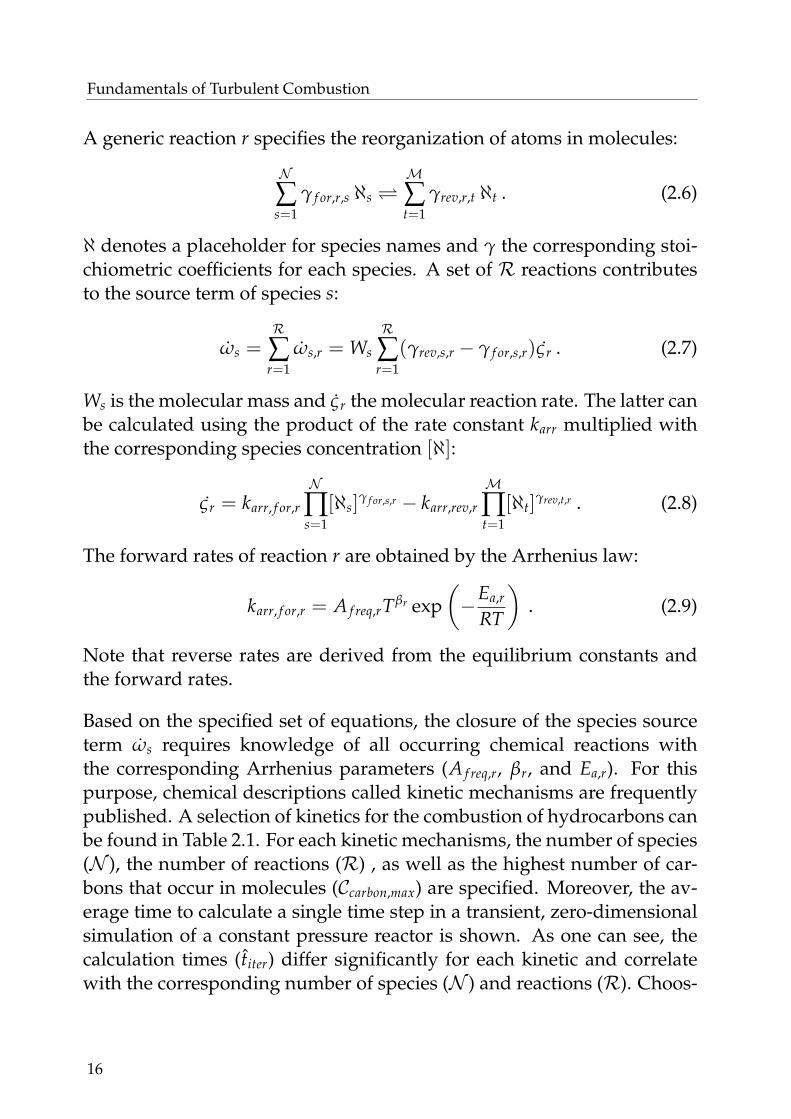
Based on the specified set of equations, the closure of the species sourceterm ωs requires knowledge of all occurring chemical reactions withthe corresponding Arrhenius parameters (A f req,r, βr, and Ea,r). For thispurpose, chemical descriptions called kinetic mechanisms are frequentlypublished. A selection of kinetics for the combustion of hydrocarbons canbe found in Table 2.1. For each kinetic mechanisms, the number of species(N ), the number of reactions (R) , as well as the highest number of car-bons that occur in molecules (Ccarbon,max) are specified. Moreover, the av-erage time to calculate a single time step in a transient, zero-dimensionalsimulation of a constant pressure reactor is shown. As one can see, thecalculation times (titer) differ significantly for each kinetic and correlatewith the corresponding number of species (N ) and reactions (R). Choos-
16
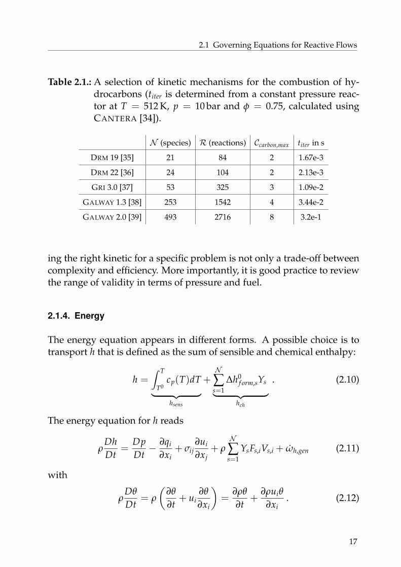
2.1 Governing Equations for Reactive Flows
Table 2.1.: A selection of kinetic mechanisms for the combustion of hy-drocarbons (titer is determined from a constant pressure reac-tor at T = 512 K, p = 10 bar and φ = 0.75, calculated usingCANTERA [34]).
N (species) R (reactions) Ccarbon,max titer in s
DRM 19 [35] 21 84 2 1.67e-3
DRM 22 [36] 24 104 2 2.13e-3
GRI 3.0 [37] 53 325 3 1.09e-2
GALWAY 1.3 [38] 253 1542 4 3.44e-2
GALWAY 2.0 [39] 493 2716 8 3.2e-1
ing the right kinetic for a specific problem is not only a trade-off betweencomplexity and efficiency. More importantly, it is good practice to reviewthe range of validity in terms of pressure and fuel.
2.1.4. Energy
The energy equation appears in different forms. A possible choice is totransport h that is defined as the sum of sensible and chemical enthalpy:
h =∫ T
T0cp(T)dT
︸ ︷︷ ︸hsens
+N∑s=1
∆h0f orm,sYs
︸ ︷︷ ︸hch
. (2.10)
The energy equation for h reads
ρDhDt
=DpDt− ∂qi
∂xi+ σij
∂ui
∂xj+ ρ
N∑s=1
YsFs,iVs,i + ωh,gen (2.11)
with
ρDθ
Dt= ρ
(∂θ
∂t+ ui
∂θ
∂xi
)=
∂ρθ
∂t+
∂ρuiθ
∂xi. (2.12)
17
Fundamentals of Turbulent Combustion
The first term on the right hand side of Equation 2.11 describes enthalpychanges due to the temporal change of pressure. The second term ex-presses enthalpy changes due to diffusion of heat or species with differ-ent enthalpies. Heating due to viscous effects is expressed by the thirdterm. Moreover, the fourth term on the right hand side describes en-thalpy changes due to volume forces. The last term ωh,gen denotes genericsources like the absorption of radiation energy. Note that Equation 2.11has no source term due to chemical rates as h is conservative1 in combus-tion. A source term describing the heat release due to combustion appearsin the sensible enthalpy form of the energy equation:
ρDhsens
Dt=
DpDt− ∂qi
∂xi+− ∂
∂xi
(ρN∑s=1
hsens,sYsVs,i
)
+ σij∂ui
∂xj+ ρ
N∑s=1
YsFs,iVs,i + ωh,ch + ωh,gen
(2.13)
with
ωh,ch = −N∑s=1
∆h0f orm,sωs . (2.14)
2.2. Modeling Turbulence
In the following, a method is presented that drastically reduces the nu-merical effort by averaging transient turbulent structures. The sectionbegins with an introduction to turbulence whereat useful quantities aredefined. Section 2.2.2 presents a set of ensemble-averaged governingequations. Here, unclosed quantities called Reynolds-stresses need to beclosed by turbulence models, which is the subject of Section 2.2.2.1.
2.2.1. Scales in Turbulent Flows
Turbulent flows feature transient, irregular and seemingly random orchaotic fluid motions as mentioned by Pope [40]. The transition from a1 In a combustion process, chemical enthalpy is converted to sensible enthalpy. Hence, the sum of both is
conservative during the combustion process.
18
2.2 Modeling Turbulence
laminar flow to a turbulent state takes place when inertial forces domi-nate viscous forces. Turbulent flows show rotating structures denoted aseddies occurring in a broad range of length scales. Technically relevantproperties of the flow are significantly impacted by turbulent structures.For instance, the mixing of two components occurs significantly slowerin laminar conditions. Unfortunately, turbulence itself is far from beingunderstood and mathematical descriptions often have a semi-empiricalcharacter. The Eddy Cascade Hypotheses by Richardson [41] (and contri-butions by Kolmogorov [42]) is a theory that describes the interaction ofeddies occuring in a broad spectrum of length scales. Richardson’s modelleads to various useful quantities that are introduced in the following.The turbulent kinetic energy k is defined by the square of the eddies cir-cumferential speed u′:
k = u′2(r) . (2.15)
Dissipation ε can be estimated by dividing k with the eddy’s circumfer-ential time:
ε =u′2(r)
τeddy(r)=
u′3(r)r
. (2.16)
In order to categorize eddies by length and energy, further quantities areintroduced in the following. The wave number w is the inverse of theeddies diameter leddy. Furthermore, the density of turbulent kinetic energyin wave number space reads
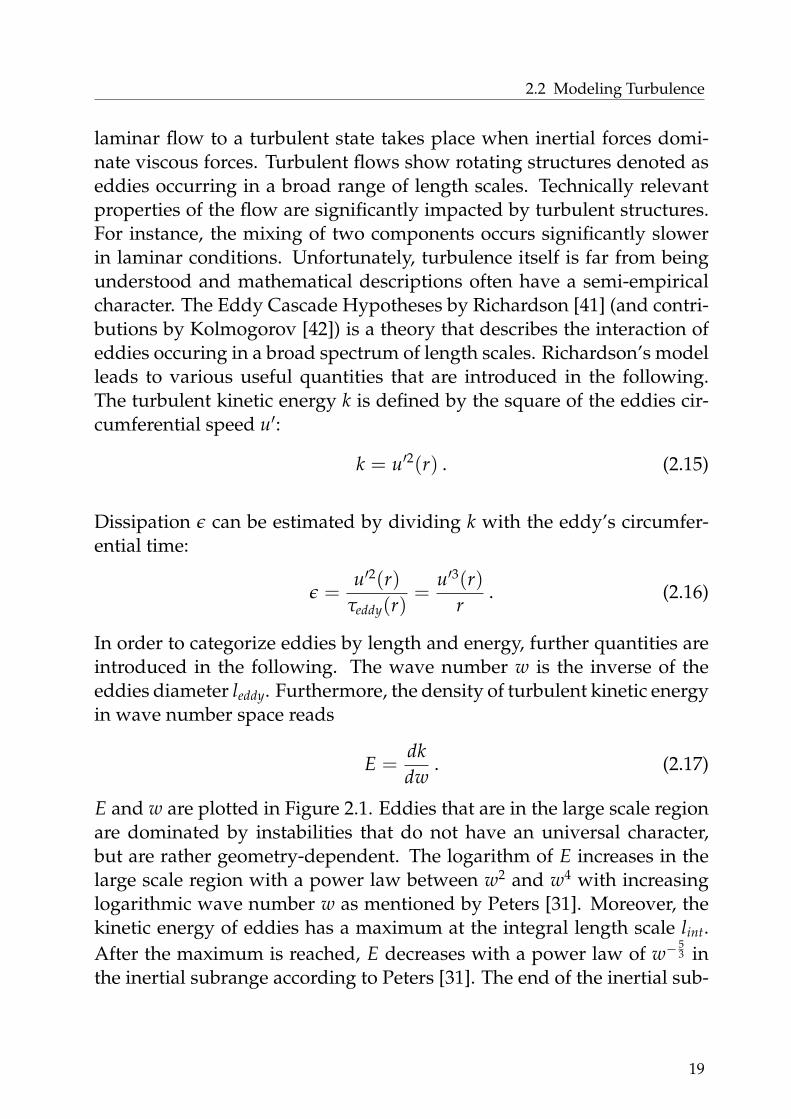
E =dkdw
. (2.17)
E and w are plotted in Figure 2.1. Eddies that are in the large scale regionare dominated by instabilities that do not have an universal character,but are rather geometry-dependent. The logarithm of E increases in thelarge scale region with a power law between w2 and w4 with increasinglogarithmic wave number w as mentioned by Peters [31]. Moreover, thekinetic energy of eddies has a maximum at the integral length scale lint.After the maximum is reached, E decreases with a power law of w−
53 in
the inertial subrange according to Peters [31]. The end of the inertial sub-
19
Fundamentals of Turbulent Combustion
l−1int η−1
largescales
integralscales
inertialsubrange
viscoussubrange
modeled in RANS
computed in DNS
computed in LES modeled in LES
wave number log(w) in log (1/m)
ener
gyde
nsit
ylo
g(E)
inlo
g( m
3 /s2)
Figure 2.1.: Turbulence energy spectrum (adapted from Peters [31] as wellas from Poinsot and Veynante [28]).
range is marked by the Kolmogorov scale η. Smaller eddies are in the vis-cous subrange in which the eddy’s energy decreases exponentially dueto viscous effects. In order to derive an expression for the Kolmogorovlength η, the Reynolds number Re is introduced that quantifies the ratioof inertial to viscous forces in a dimensionless way:
Re(r) =u′(r)r
ν. (2.18)
The following expression to evaluate the Kolmogorov length η is derivedby assuming that the viscous subrange starts when viscous forces equalinertial forces:
Re(η) =u′(η)η
ν= 1 −→ η =
ν
u′(η). (2.19)
20
2.2 Modeling Turbulence
2.2.2. Reynolds-Averaged Governing Equations for Reactive Flows
Solving the instantaneous governing equations of Section 2.1 is denotedas Direct Numerical Simulation (DNS). DNS resolves even the small-est turbulent structures that requires vast computational grids leadingto high computational effort. Thus, DNS is up to now limited to fewacademic resource activities, small geometries, and low Reynolds num-bers. In Large Eddy Simulations (LES), only the turbulent structures thatare above a specified threshold are resolved. Below this limit, the aver-aged values are determined by subgrid models. A third approach calledReynolds-Averaged Navier-Stokes (RANS) solves solely the mean valuesof all turbulent structures. This leads to a significant reduction of calcula-tion time and makes it furthermore possible to employ two-dimensionalgeometries and symmetric or periodic boundary conditions. A furtheradvantage of RANS is the possibility to evaluate a single stationary stateinstead of solving a time series. Note that all methods developed in thiswork are based on RANS, which is introduced in the following. Ensembleaveraging denotes the split of an arbitrary quantity θ into a mean and afluctuating part:
θ = θ + θ′ . (2.20)
Using the standard RANS equations based on ensemble averaging leadto specific challenges in flows of non-constant density. Hence, solversusually employ the mass-weighted mean introduced by Favre [43]. AFavre-averaged generic variable is defined by
θ =ρθ
ρ. (2.21)
In addition, fluctuations of θ are separated:
θ = θ + θ′′ with θ′′ = 0 . (2.22)
21
Fundamentals of Turbulent Combustion
The Favre-averaged governing equations for mass, momentum, species,and energy read2
∂ρ
∂t+
∂ρui
∂xi= 0 , (2.23)
∂ρuj
∂t+
∂ρuiuj
∂xi+
∂p∂xj
=∂
∂xi
(σij − ρu′′i u′′j
), (2.24)
∂ρYs
∂t+
∂ρuiYs
∂xi= − ∂
∂xiρ(
u′′i Y′′s + Vs,iYs
)+ ωs , (2.25)
and∂ρhsens
∂t+
∂ρuihsens
∂xi=
DpDt
− ∂
∂xi
(ρu′′i h′′sens + ρ
N
∑s=1
hsens,sVs,iYs − qi
)
+ σij∂ui
∂xj+ ωh,ch + ωh,gen
(2.26)
with
DpDt
=∂p∂t
+ ui∂p∂xi
+ u′′i∂p∂xi
. (2.27)
Here, several unclosed terms appear: Reynolds-stresses u′′i u′′j , turbulentmass fluxes u′′i Y′′s , and turbulent enthalpy flux u′′i h′′sens. The modeling ofthese terms is introduced in the following. Furthermore, the ensemble-averaged species source term ωs is closed by combustion models, whichis the subject of Section 2.3. A further unclosed term is the ensemble-averaged product of velocity fluctuation and spatial pressure gradientu′′i ∂p/∂xi appearing in Equation 2.27. This term is usually small and oftenneglected as mentioned by Poinsot and Veynante [28].
2 Volume forces have been neglected for the sake of clarity.
22
2.2 Modeling Turbulence
2.2.2.1. Modeling Reynolds Stresses
The Reynolds stresses are closed by turbulence models that are oftenbased on the approximation by Boussinesq [44]:
ρu′′i u′′j ≈ ρu′′i u′′j ≈ −µt
(∂ui
∂xj+
∂uj
∂xi− 2
3δij
∂uk
∂xk
)+
23
ρk . (2.28)
Here, the turbulent dynamic viscosity µt appears and requires closure.Due to the technical relevance, a variety of semi-empirical models havebeen published. The popular k-ε by Jones and Launder [45] is introducedin the following. The k-ε model uses two transport equations to determinek and ε. With the knowledge of both quantities, µt can be estimated usingthe following approximation:
µt = ρCµk2
ε(2.29)
∂ρk∂t
+∂ρuik
∂xi=
∂
∂xi
(∂k∂xi
(µ +
µt
Cσ
))+ Pk − ρε (2.30)
∂ρε
∂t+
∂ρuiε
∂xi=
∂
∂xi
(∂ε
∂xi
(µ +
µt
Cε
))+ Cε,1
ε
kPk − Cε,2ρ
ε2
k. (2.31)
Cµ, Cε, Cε,1, Cε,2, Cσ are model constants. Moreover, Pk reads
Pk = − ρu′′i u′′j︸ ︷︷ ︸Boussinesq
∂ui
∂xj. (2.32)
2.2.2.2. Modeling Fluxes
As discussed above, simulations based on RANS do not resolve turbulentstructures. Thus, turbulent fluxes are unknown and require modeling.These terms appear in Equation 2.25 and 2.26 in the form of u′′i Y′′s and u′′i h′′sens.
23
Fundamentals of Turbulent Combustion
A popular way to treat turbulent fluxes of an arbitrary scalar θ is to usethe gradient assumption:
ρu′′i θ′′ = − µt
Sct,θ
∂θ
∂xi. (2.33)
Here, the turbulent Schmidt number appears that reads
Sct,θ =µt
Dt,θ. (2.34)
Dt,θ can be interpreted as a mass diffusion coefficient of θ due to turbu-lence. In the present work, a constant Schmidt number of 0.7 is used. Thepotential significance of this simplification is discussed by Veynante et al.[46].
Note that molecular diffusion is usually significantly smaller than turbu-lent fluxes and hence often neglected.
2.3. Modeling Combustion
In the following, the theoretical fundamentals of turbulent (partially)premixed combustion are covered. The first section shows a freely-propagating flamelet3. Furthermore, the mechanisms of stretched flamespropagating in moving flows are presented in Section 2.3.2. Section 2.3.3discusses flames in turbulent environments and introduces a methodto classify turbulent premixed combustion regarding the turbulence-chemistry interaction. In Section 2.3.4, a selection of standard combustionmodels is introduced.
2.3.1. Freely-Propagating Flames
Premixed combustion requires fuel and oxidizer to be perfectly mixed onthe molecular level prior to combustion. In contrast to diffusion flames,the reaction rate is not limited by the molecular transport of fuel and oxi-
3 The term freely propagating indicates that there is no aerodynamic interaction between combustion andflow. in order to introduce basic principles of combustion.
24
2.3 Modeling Combustion
dizer. The global fuel to oxidizer ratio can be defined by the equivalenceratio φ, which reads
φ = bYf uel
Yoxidwith b =
Yoxid
Yf uel
∣∣∣∣sto
. (2.35)
Note that this definition cannot be evaluated in the exhaust gas. For aglobally valid evaluation, a combustion conservative definition is needed.A popular choice is the mixture fraction f , which reads
f =bYf uel −Yoxid + Yoxid,u
bYf uel,u + Yoxid,u. (2.36)
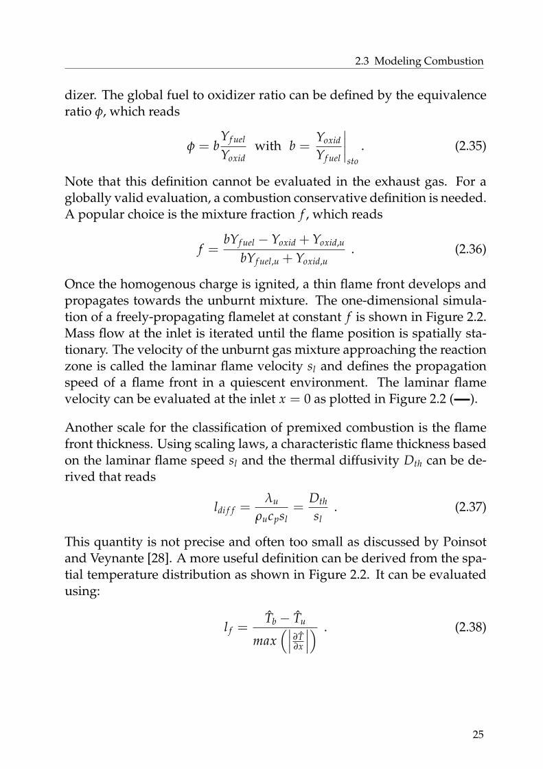
Once the homogenous charge is ignited, a thin flame front develops andpropagates towards the unburnt mixture. The one-dimensional simula-tion of a freely-propagating flamelet at constant f is shown in Figure 2.2.Mass flow at the inlet is iterated until the flame position is spatially sta-tionary. The velocity of the unburnt gas mixture approaching the reactionzone is called the laminar flame velocity sl and defines the propagationspeed of a flame front in a quiescent environment. The laminar flamevelocity can be evaluated at the inlet x = 0 as plotted in Figure 2.2 ( ).
Another scale for the classification of premixed combustion is the flamefront thickness. Using scaling laws, a characteristic flame thickness basedon the laminar flame speed sl and the thermal diffusivity Dth can be de-rived that reads
ldi f f =λu
ρucpsl=
Dth
sl. (2.37)
This quantity is not precise and often too small as discussed by Poinsotand Veynante [28]. A more useful definition can be derived from the spa-tial temperature distribution as shown in Figure 2.2. It can be evaluatedusing:
l f =Tb − Tu
max(∣∣∣ ∂T
∂x
∣∣∣) . (2.38)
25

Fundamentals of Turbulent Combustion
1 2 3 4 5
·10−4
0
sl/umax
1
l f
x space in m
norm
aliz
edax
is
T ≈ uc
0
0.1
0.2
spec
ies
mas
sfr
acti
onYCH4
O2CO2CO
Figure 2.2.: Spatial profiles of selected quantities (freely-propagating atT = 512 K, p = 10 bar and φ = 0.75, calculated using GAL-WAY 1.3 [38] and CANTERA [34]).
Furthermore, the reaction progress c is plotted in Figure 2.2 ( ). c de-termines the progress of the combustion process from zero to unity. Thefollowing definition for c can be employed for the combustion of hydro-carbons:
c =(YCO−YCO,u) +
(YCO2
−YCO,u)
(YCO,eq −YCO,u
)+(YCO2,eq −YCO,u
) . (2.39)
The second y-axis of Figure 2.2 represents the mass fraction of four se-lected species. Fuel consists of pure CH4 ( ) and the oxidizer is dioxy-gen (O2, ). Both species decrease over the reaction zone as they convertto species of lower energetic level by releasing heat. The carbon atomstake various paths and pass numerous intermediate species before theyeventually react to CO2 ( ) . Since almost every C-atom has to pass CO( ), a maximum develops within the flame.
26

2.3 Modeling Combustion
2.3.2. Stretched Flames in Moving Environments
The flame shown in Figure 2.2 propagates in a quiescent environment(freely propagating). In reality, flames are usually exposed to multidi-mensional velocity fields. The aerodynamic effect of a moving flow onthe flame is called flame stretch. It is defined by the temporal change of aflame surface element A f :
κ =1
A f
dA f
dt. (2.40)
Stretching a flame leads to steeper gradients that may significantly impactthe flame speed due to the following mechanisms:
• Feeding the flame with more fuel, causing the flame speed to in-crease.
• Cooling the flame as the diffusion of heat towards the unburnt mate-rial is increased, leading to a decrease in flame speed.
Note that both mechanisms are superimposed. Hence, the effect of stretchon flame speed is ambiguous as acceleration or deceleration is possible. Ageneral expression for flame stretch κ can be derived from Equation 2.40by using Reynold’s transport theorem as shown by Poinsot and Veynante[28]. Flame stretch in index notation reads
κ = (δij − ninj)∂ui
∂xj︸ ︷︷ ︸κst
+ sd∂ni
∂xi︸ ︷︷ ︸κcurv
. (2.41)
It is useful to write this equation without indices. For this purpose, a localcoordinate system that is normal to the flame surface is introduced. Flamestretch then reads
κ = ∇ · u− (n⊗ n) : ∇u︸ ︷︷ ︸κst
+ sd∇ · n︸ ︷︷ ︸κcurv
. (2.42)
The displacement speed sd defines the flame front velocity relative to theflow in normal direction (n). The first two terms on the right hand side
27

Fundamentals of Turbulent Combustion
n
x
y
dA f
r1
r2
Lines SurfacesFont
Fehn allg.
Fehn
Figure 2.3.: Visualization of the local orthonormal basis on the left handside and two radii describing curvature on the right handside.
of Equation 2.42 express strain. Strain is defined as the volume changeof a fluid element minus the part that is normal to the surface and can beinterpreted as the flow acceleration in a plane that is parallel to the flamesurface. The plane can be defined by two vectors x and y as shown inFigure 2.3. Equation 2.42 can then be rewritten:
κ = (x⊗ x + y⊗ y) : ∇u + sd∇ · n . (2.43)
As depicted on the right hand side of Figure 2.3, curvature of the flamefront can be described by two radii:
κ = (x⊗ x + y⊗ y) : ∇u− sd
(1r1
+1r2
). (2.44)
2.3.3. Premixed Flames in Turbulent Conditions
As mentioned before, turbulence itself is complex, difficult to model andstill not fully understood. This naturally also applies to the interactionof turbulence with chemistry in turbulent combustion. A prerequisite ofcombustion is mixing on the molecular level of unburnt and burnt ma-terial for premixed combustion or fuel and oxidizer for non-premixedcombustion. The general understanding is that this mixing process oc-
28
2.3 Modeling Combustion
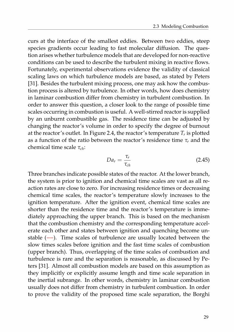
curs at the interface of the smallest eddies. Between two eddies, steepspecies gradients occur leading to fast molecular diffusion. The ques-tion arises whether turbulence models that are developed for non-reactiveconditions can be used to describe the turbulent mixing in reactive flows.Fortunately, experimental observations evidence the validity of classicalscaling laws on which turbulence models are based, as stated by Peters[31]. Besides the turbulent mixing process, one may ask how the combus-tion process is altered by turbulence. In other words, how does chemistryin laminar combustion differ from chemistry in turbulent combustion. Inorder to answer this question, a closer look to the range of possible timescales occurring in combustion is useful. A well-stirred reactor is suppliedby an unburnt combustible gas. The residence time can be adjusted bychanging the reactor’s volume in order to specify the degree of burnoutat the reactor’s outlet. In Figure 2.4, the reactor’s temperature Tr is plottedas a function of the ratio between the reactor’s residence time τr and thechemical time scale τch:
Dar =τr
τch(2.45)
Three branches indicate possible states of the reactor. At the lower branch,the system is prior to ignition and chemical time scales are vast as all re-action rates are close to zero. For increasing residence times or decreasingchemical time scales, the reactor’s temperature slowly increases to theignition temperature. After the ignition event, chemical time scales areshorter than the residence time and the reactor’s temperature is imme-diately approaching the upper branch. This is based on the mechanismthat the combustion chemistry and the corresponding temperature accel-erate each other and states between ignition and quenching become un-stable ( ). Time scales of turbulence are usually located between theslow times scales before ignition and the fast time scales of combustion(upper branch). Thus, overlapping of the time scales of combustion andturbulence is rare and the separation is reasonable, as discussed by Pe-ters [31]. Almost all combustion models are based on this assumption asthey implicitly or explicitly assume length and time scale separation inthe inertial subrange. In other words, chemistry in laminar combustionusually does not differ from chemistry in turbulent combustion. In orderto prove the validity of the proposed time scale separation, the Borghi
29
Fundamentals of Turbulent Combustion
Dar,q Dar,ign
Damkohler number Dar
reac
tor’
ste
mer
atur
eT r
Figure 2.4.: Temperature in a well-stirred reactor as a function ofDamkohler number (adapted from Peters [31]).
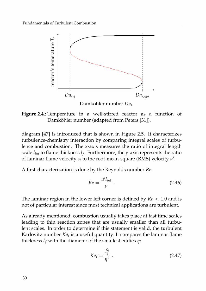
diagram [47] is introduced that is shown in Figure 2.5. It characterizesturbulence-chemistry interaction by comparing integral scales of turbu-lence and combustion. The x-axis measures the ratio of integral lengthscale lint to flame thickness l f . Furthermore, the y-axis represents the ratioof laminar flame velocity sl to the root-mean-square (RMS) velocity u′.
A first characterization is done by the Reynolds number Re:
Re =u′lint
ν. (2.46)
The laminar region in the lower left corner is defined by Re < 1.0 and isnot of particular interest since most technical applications are turbulent.
As already mentioned, combustion usually takes place at fast time scalesleading to thin reaction zones that are usually smaller than all turbu-lent scales. In order to determine if this statement is valid, the turbulentKarlovitz number Kat is a useful quantity. It compares the laminar flamethickness l f with the diameter of the smallest eddies η:
Kat =l2
f
η2 . (2.47)
30

2.3 Modeling Combustion
laminar wrinkled flamelets
corrugated flamelets
Kat =100
rati
oof
velo
city
scal
esu′
/sl
ratio of length scales lint/l f
thin reaction zones
disrupted flames
Kat =1
1e0
1e1
1e2
1e3
1e-1 1e0 1e1 1e2 1e3
Re = 1
Lines SurfacesFont
Figure 2.5.: Classification of turbulence-chemistry interaction in theBorghi diagram (adapted from Peters [31] as well as Poinsotand Veynante [28]).
The idea behind this comparison is illustrated in Figure 2.6. Based on Kat,three regions in the Borghi diagram are identified:
• Corrugated and wrinkled flamelets: If Kat is below unity, the small-est eddies do not penetrate the flamelets. Nevertheless, aerodynamicinteractions may occur, leading to wrinkling and stretching of theflame sheet.
• Thin reaction zones: For values of Kat that are above unity, eddiespenetrate the flame and interact with the preheat zone. As a conse-quence, the flame front is thickened. Note that the criterion Kat > 1
31
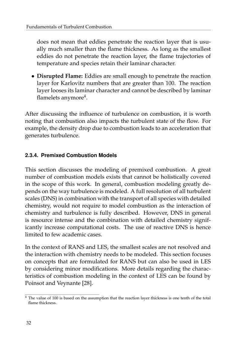
Fundamentals of Turbulent Combustion
does not mean that eddies penetrate the reaction layer that is usu-ally much smaller than the flame thickness. As long as the smallesteddies do not penetrate the reaction layer, the flame trajectories oftemperature and species retain their laminar character.
• Disrupted Flame: Eddies are small enough to penetrate the reactionlayer for Karlovitz numbers that are greater than 100. The reactionlayer looses its laminar character and cannot be described by laminarflamelets anymore4.
After discussing the influence of turbulence on combustion, it is worthnoting that combustion also impacts the turbulent state of the flow. Forexample, the density drop due to combustion leads to an acceleration thatgenerates turbulence.
2.3.4. Premixed Combustion Models
This section discusses the modeling of premixed combustion. A greatnumber of combustion models exists that cannot be holistically coveredin the scope of this work. In general, combustion modeling greatly de-pends on the way turbulence is modeled. A full resolution of all turbulentscales (DNS) in combination with the transport of all species with detailedchemistry, would not require to model combustion as the interaction ofchemistry and turbulence is fully described. However, DNS in generalis resource intense and the combination with detailed chemistry signif-icantly increase computational costs. The use of reactive DNS is hencelimited to few academic cases.
In the context of RANS and LES, the smallest scales are not resolved andthe interaction with chemistry needs to be modeled. This section focuseson concepts that are formulated for RANS but can also be used in LESby considering minor modifications. More details regarding the charac-teristics of combustion modeling in the context of LES can be found byPoinsot and Veynante [28].
4 The value of 100 is based on the assumption that the reaction layer thickness is one tenth of the totalflame thickness.
32
2.3 Modeling Combustion
Kat = 1
Kat = 100
reactionlayer
preheatzone
unburnt
burnt
kolmogoroveddies
turbulentflame brush
Lines SurfacesFont
Figure 2.6.: Visualization of the interaction of eddies with a flame front.
In the following, a selection of three different combustion models are in-troduced. The first two models are based on the transport of species anddiffer significantly in the way the species source terms are closed. Whilethe first model assumes that only chemical finite rates (FR) are the limit-ing factor, the second model states that turbulent mixing is always slowerthan all chemical scales. Furthermore, the Turbulent Flame Speed Closure(TFC) is introduced that is based on the transport of control variables in-stead of species. Note that the first model (FR) is introduced for didacticreasons only while the second and third model are used to benchmark thein Chapter 3 introduced combustion modeling strategy.
Note that some popular models are not covered in this section. For in-stance, the concept of Probability Density Functions (PDF) to describe thedistribution of species and/or reaction progress is subject of Chapter 3.Two other worth mentioning models are the Bray Moss Libby concept
33
Fundamentals of Turbulent Combustion
and the Flame Surface Density Model. An introduction to these modelscan be found by Poinsot and Veynante [28].
2.3.4.1. Finite Rate
Assuming that chemistry is the limiting rate, the most intuitive approachwould be to close the ensemble-averaged species source term ωs by sum-ming up all corresponding reactions:
ωs =R∑r=1
ωr,s (2.48)
The problem with this closure is not easy to grasp but important to notein the scope of the present work. Equation 2.48 closes the ensemble-averaged species source term by a chemical model that does not con-sider any fluctuations of temperature and species. Mean values, likethe Favre-averaged temperature, represent a variety of different instanta-neous physicochemical states. In specific situations, high variances mayeven indicate that the statistical probability for the mean value is closeto zero. It is hence questionable to calculate a species source term withaveraged quantities in a model that requires instantaneous values. Theevaluation of the source term would only be valid if one or both of thefollowing conditions are true:
1. The source term as a function of temperature and species have a lin-ear character.
2. Fluctuations are close to zero.
Both conditions are usually not present in turbulent combustion pro-cesses.
2.3.4.2. Eddy Break-Up Model
The Eddy Break-Up (EBU) model published by Spalding [48, 49] statesthat combustion is solely a function of turbulence for the often valid as-sumption of high Reynolds and Damkohler numbers. The idea is that
34
2.3 Modeling Combustion
turbulent eddies transport either burnt or unburnt gases and that mixingof both materials solely scales with the time scales of turbulent mixing.The source term for a product species s reads
ωs = ρCebuε
k
√Y′′2s . (2.49)
The EBU model is popular due to its simplicity and often leads to more ac-curate results than the FR model, as mentioned by Poinsot and Veynante[28]. However, Peters [31] states that the use of EBU often requires exces-sive model tuning to achieve accurate heat release distributions. Due tothe negligence of possible finite rate limitations, EBU is not able to con-sider the impact of various equivalence ratios φ or different fuel compo-sitions. It is evident that the prediction of the critical equivalence ratio forlean blowout by EBU is not advisable.
A qualitative comparison of the ensemble-averaged reaction rate pre-dicted by EBU ( ) and FR ( ) can be found in Figure 2.7. The in-tense peak from the FR model is characteristic due to the previously dis-cussed self-accelerating character of combustion after the temperature hasreached a critical value. Moreover, EBU solely scales with the fluctua-tion of the product mass fraction that has a maximum when the Favre-averaged temperature is increased by 50 % of the total temperature eleva-tion.
The Eddy Dissipation Model (EDM) is an improved version of EBU byMagnussen and Hjertager [50]. In EDM, the variance Y′′2s is replaced bythe mean species mass fraction in order to consider the influence of equiv-alence ratio.
2.3.4.3. Turbulent Flame Speed Closure
The flamelet theory assumes that chemistry is fast leading to infinitelythin reaction zones. Furthermore, the flamelet is fluctuating in a zone thatis called the turbulent flame brush as illustrated in Figure 2.6. Note thatthe flamelet fluctuations are transient and depend on turbulent structuresthat are not resolved in RANS simulations. RANS do rather resolve thestatistical mean of the reaction progress in order to determine the position
35
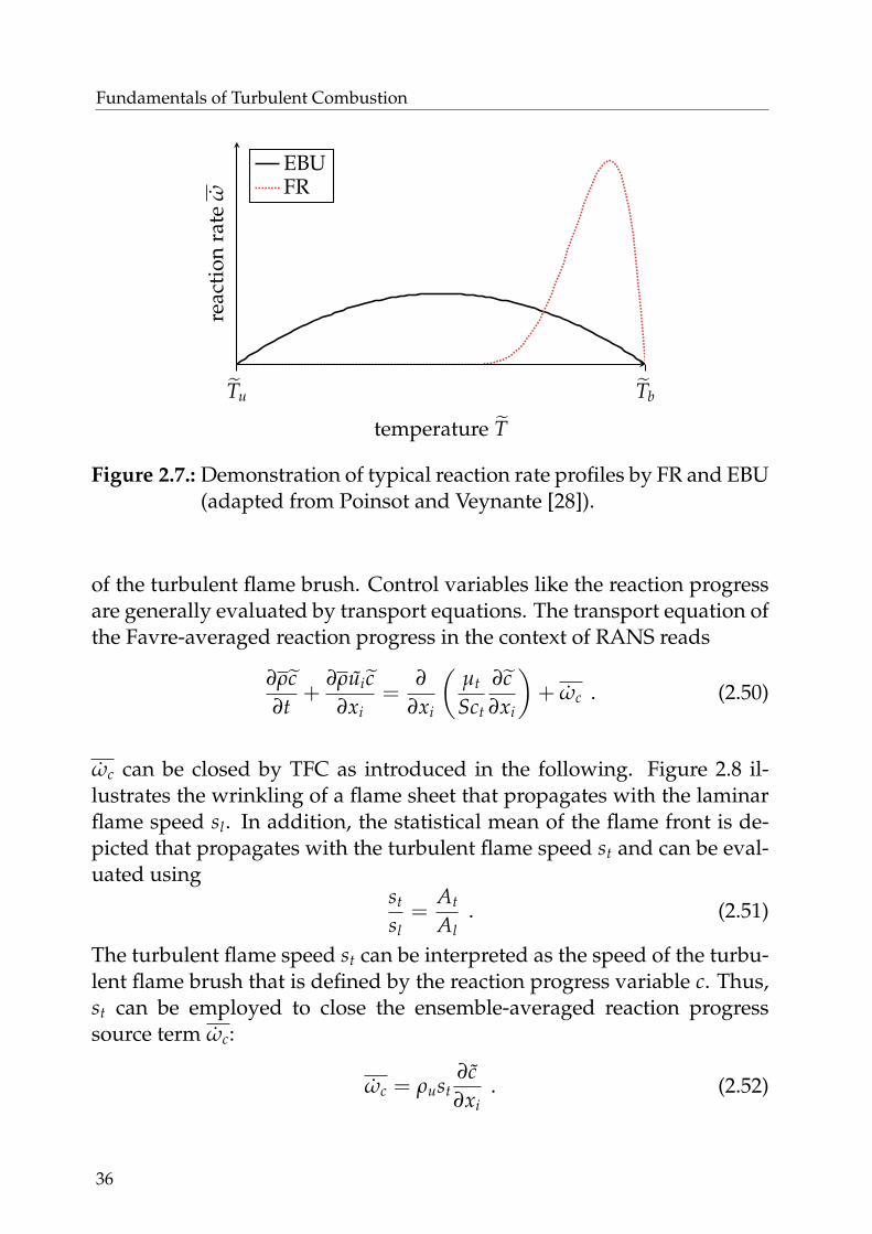
Fundamentals of Turbulent Combustion
Tu Tb
temperature T
reac
tion
rate
ω
EBUFR
Figure 2.7.: Demonstration of typical reaction rate profiles by FR and EBU(adapted from Poinsot and Veynante [28]).
of the turbulent flame brush. Control variables like the reaction progressare generally evaluated by transport equations. The transport equation ofthe Favre-averaged reaction progress in the context of RANS reads
∂ρc∂t
+∂ρuic∂xi
=∂
∂xi
(µt
Sct
∂c∂xi
)+ ωc . (2.50)
ωc can be closed by TFC as introduced in the following. Figure 2.8 il-lustrates the wrinkling of a flame sheet that propagates with the laminarflame speed sl. In addition, the statistical mean of the flame front is de-picted that propagates with the turbulent flame speed st and can be eval-uated using
st
sl=
At
Al. (2.51)
The turbulent flame speed st can be interpreted as the speed of the turbu-lent flame brush that is defined by the reaction progress variable c. Thus,st can be employed to close the ensemble-averaged reaction progresssource term ωc:
ωc = ρust∂c∂xi
. (2.52)
36
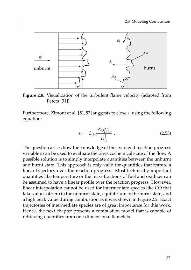
2.3 Modeling Combustion
m
sl
st
Al
At
Lines SurfacesFont
./2-Fun/Figures/Duct/./2-Fun/Figures/Duct/duct.pdf
unburnt burnt
Figure 2.8.: Visualization of the turbulent flame velocity (adapted fromPeters [31]).
Furthermore, Zimont et al. [51,52] suggests to close st using the followingequation:
st = Ct f cu′
34 s
12l l
14int
D14th
. (2.53)
The question arises how the knowledge of the averaged reaction progressvariable c can be used to evaluate the physicochemical state of the flow. Apossible solution is to simply interpolate quantities between the unburntand burnt state. This approach is only valid for quantities that feature alinear trajectory over the reaction progress. Most technically importantquantities like temperature or the mass fractions of fuel and oxidizer canbe assumed to have a linear profile over the reaction progress. However,linear interpolation cannot be used for intermediate species like CO thattake values of zero in the unburnt state, equilibrium in the burnt state, anda high peak value during combustion as it was shown in Figure 2.2. Exacttrajectories of intermediate species are of great importance for this work.Hence, the next chapter presents a combustion model that is capable ofretrieving quantities from one-dimensional flamelets.
37


3 Modeling Combustion
A combustion model is presented in this chapter that is designed to fea-ture high accuracy in cold conditions. The modeling strategy is based onFGM that was initially proposed by van Oijen et al. [53, 54]. An intro-duction to FGM for the application in turbulent, partially-premixed con-ditions is given in the first section of this chapter. Moreover, Section 3.2presents a novel approach to efficiently consider flame stretch and heatloss. In Section 3.3, the developed models are applied to an atmosphericsingle-burner test rig in order to validate the numerically predicted heatrelease distribution. The chapter concludes with Section 3.4 in which stan-dard combustion models are compared with the proposed modeling strat-egy.
3.1. Flamelet Generated Manifolds
The basic principle of FGM is to look up physicochemical quantities intables that are generated by one-dimensional flamelet simulations basedon detailed chemistry and advanced diffusion models. The tables areparametrized by control variables that must be evaluated by additionaltransport equations. FGM has advantages in comparison to other chem-istry reduction methods like the Intrinsic Low-Dimensional Manifolds(ILDM) model by Maas and Pope [55] as stated by van Oijen [54]. ILDMuses the steady-state assumption for fast reactions and can thus be inac-curate in cold regions that are limited by slow chemistry. Furthermore, adecisive advantage of FGM is that species trajectories are accurately de-scribed by the flamelet-generated manifolds. This is of great importancefor this work, as the modeling of CO is based on the correct representationof intermediate species within the turbulent flame brush. An applicationof FGM to partially-premixed combustion can be found by Ramaekers etal. [56]. In partially-premixed combustion with binary mixtures, the com-
39
Modeling Combustion
bination of the reaction progress variable c and the mixture fraction f is areasonable choice. In general, a Favre-averaged control variable θ can betransported using
∂ρθ
∂t+
∂ρuiθ
∂xi=
∂
∂xi
(µt
Sct
∂θ
∂xi
)+ ωθ . (3.1)
As mentioned before, the transport of the reaction progress c requiresmodeling of the source term ωc. In the context of FGM, ωc is retrievedfrom manifolds. The look up of tabulated quantities by solely usingFavre-averaged control variables would be inaccurate due to the non-linear character of combustion chemistry as discussed in Section 2.3.4.1.The turbulent fluctuations of the control variables require to consider ev-ery possible state with its respective probability. For this purpose, PDFsP are used to describe the statistical distribution of the control variables.The statistical mean of a looked-up quantity results from the integrationof the product of the scalar and its statistical distribution:
ω0c =
∫∫ω0
c (c, f )P(c, f ) dc d f . (3.2)
Joint PDFs of statistically independent control variables can be calculatedby multiplying the corresponding marginal PDFs. A marginal PDF is thedistribution of a single control variable. Assuming that c and f are inde-pendent, the joint PDF can be calculated using:
P(c, f ) = P(c)P( f ) . (3.3)
Various strategies for determining marginal PDF shapes for scalars in tur-bulent flows have been published. One option is to presume a specificfunction for the PDF. The shape of this function can be modeled usingthe mean and the variance of the control variable (first two conditionalmoments):
ω0c (c, c′′, f , f ′′) =
∫∫ω0
c (c, f )P(c, c, c′′)P( f , f , f ′′) dc d f . (3.4)
The variances c′′ and f ′′ are usually evaluated by additional transportequations. It is important to note that presumed PDFs are a significantsimplification since the actual distribution may substantially differ from
40
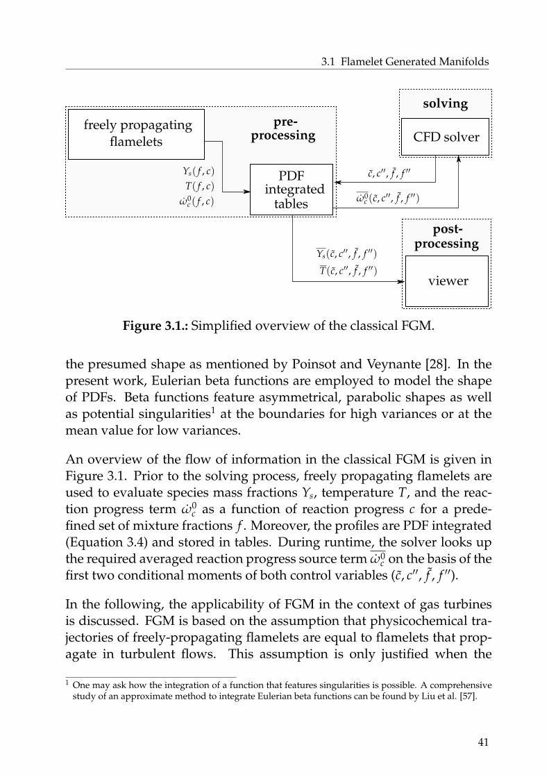
3.1 Flamelet Generated Manifolds
f
κstψ
f , κ, ψ s∗c(κ, ψ, f
)
Γ(s∗c , s0c)
s0c(
f)
additional manifold
computationalgrid
Ys( f , c)T( f , c)
ω0c ( f , c)
PDFintegrated
Ys(c, c′′, f , f ′′)
T(c, c′′, f , f ′′)
ω0c (c, c′′, f , f ′′)
c, c′′, f , f ′′
CFD solver
viewer
freely propagating
tables
pre-
post-processing
flamelets
solving
processing
Figure 3.1.: Simplified overview of the classical FGM.
the presumed shape as mentioned by Poinsot and Veynante [28]. In thepresent work, Eulerian beta functions are employed to model the shapeof PDFs. Beta functions feature asymmetrical, parabolic shapes as wellas potential singularities1 at the boundaries for high variances or at themean value for low variances.
An overview of the flow of information in the classical FGM is given inFigure 3.1. Prior to the solving process, freely propagating flamelets areused to evaluate species mass fractions Ys, temperature T, and the reac-tion progress term ω0
c as a function of reaction progress c for a prede-fined set of mixture fractions f . Moreover, the profiles are PDF integrated(Equation 3.4) and stored in tables. During runtime, the solver looks upthe required averaged reaction progress source term ω0
c on the basis of thefirst two conditional moments of both control variables (c, c′′, f , f ′′).
In the following, the applicability of FGM in the context of gas turbinesis discussed. FGM is based on the assumption that physicochemical tra-jectories of freely-propagating flamelets are equal to flamelets that prop-agate in turbulent flows. This assumption is only justified when the
1 One may ask how the integration of a function that features singularities is possible. A comprehensivestudy of an approximate method to integrate Eulerian beta functions can be found by Liu et al. [57].
41

Modeling Combustion
smallest turbulent scales are larger than the reaction layer. In order totest the validity of this assumption, gas turbines and the employed val-idation case by Marosky [58] are investigated using the Borghi diagram.This approach requires the estimation of scales that describe combustionand turbulence. Velocity and thicknesses of flamelets are obtained fromone-dimensional calculations. Furthermore, turbulent scales are deter-mined in a CFD simulation of the validation case. Note that the burnersize and flow velocity of Marosky’s validation case is comparable to realgas turbine combustors. It is hence reasonable to assume that similarintegral length scales and RMS velocities occur in gas turbines. In thisstudy, gas turbines are considered to operate in a range of equivalenceratios between φ = 0.5 to φ = 0.8 and pressures between p = 15 bar top = 30 bar. Furthermore, the ranges of pressure and equivalence ratio areeach discretized by four points resulting in a grid of 16 operating points.The estimated scales are summarized in Table 3.1 and plotted in Figure3.2. The atmospheric validation case is located in the thin reaction zonesregime. Peters [31] states that the one-dimensional laminar character ofthe flamelet is not altered in the thin reaction zones regime. This is dueto the fact that eddies are too large to penetrate the reaction layer. More-over, the specified operational window of gas turbines is almost entirelyin the thin reaction zones regime and solely crosses the Kat = 100 limitin lean conditions at low pressure, as depicted in Figure 3.2. Note thatthe Kat = 100 line should not be seen as a strict criterion for flamelet dis-ruption as mentioned by Peters [59]. It can be concluded that the use offlamelets to describe combustion is valid for the investigated conditions.
3.2. Modeling Flame Stretch and Heat Loss
The classic way of employing freely-propagating flamelets for the gener-ation of manifolds may be problematic when it comes to flame stretch asmentioned by van Oijen and de Goey [60]. Furthermore, non-adiabatic ef-fects may also have a significant impact on the combustion process. Botheffects are not considered in the original formulation of FGM. Donini et al.[61, 62] present an example for the extension of the look up table to takeheat loss into account. Unfortunately, the addition of further dimensions
42

3.2 Modeling Flame Stretch and Heat Loss
Table 3.1.: Overview of estimated scales that occur in gas turbines and inMarosky’s [58] validation case.
φ = 0.5 φ = 0.8
sl in cm/s l f in µm sl in cm/s l f in µm lint u′
validation case at 1 bar 57 560 - -
7.1 mm 13.3 m/sgas turbine at 15 bar 15 130 52 49
gas turbine at 30 bar 22 69 68 24
laminar wrinkled flamelets
corrugated flamelets
Kat =100
ratio of length scales lint/l f
disrupted flames
Kat =1
Re = 1
Lines SurfacesFont
case
φ = 0.5
φ = 0.8
p = 15 barp = 30 barthin reaction zones
validation
rati
oof
velo
city
scal
esu′
/sl
1e0
1e1
1e2
1e3
1e-1 1e0 1e1 1e2 1e3
Figure 3.2.: Justifying the flamelet theory for Marosky’s [58] validationcase as well as for gas turbines (Borghi diagram adapted fromPeters [31] and from Poinsot and Veynante [28]).
43
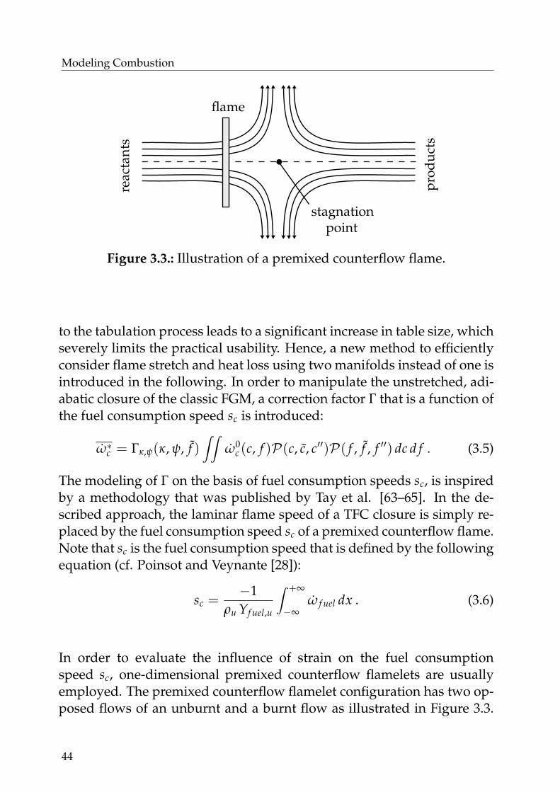
Modeling Combustion
flame
stagnation
reac
tant
s
prod
ucts
point
Figure 3.3.: Illustration of a premixed counterflow flame.
to the tabulation process leads to a significant increase in table size, whichseverely limits the practical usability. Hence, a new method to efficientlyconsider flame stretch and heat loss using two manifolds instead of one isintroduced in the following. In order to manipulate the unstretched, adi-abatic closure of the classic FGM, a correction factor Γ that is a function ofthe fuel consumption speed sc is introduced:
ω∗c = Γκ,ψ(κ, ψ, f )∫∫
ω0c (c, f )P(c, c, c′′)P( f , f , f ′′) dc d f . (3.5)
The modeling of Γ on the basis of fuel consumption speeds sc, is inspiredby a methodology that was published by Tay et al. [63–65]. In the de-scribed approach, the laminar flame speed of a TFC closure is simply re-placed by the fuel consumption speed sc of a premixed counterflow flame.Note that sc is the fuel consumption speed that is defined by the followingequation (cf. Poinsot and Veynante [28]):
sc =−1
ρu Yf uel,u
∫ +∞
−∞ω f uel dx . (3.6)
In order to evaluate the influence of strain on the fuel consumptionspeed sc, one-dimensional premixed counterflow flamelets are usuallyemployed. The premixed counterflow flamelet configuration has two op-posed flows of an unburnt and a burnt flow as illustrated in Figure 3.3.
44

3.2 Modeling Flame Stretch and Heat Loss
Equilibration2 of the reactants is accomplished in order to determine thethermodynamic state of the burnt gas. The laminar flame speed sl equalsthe fuel consumption speed sc for zero strain rates and without heat loss.A decisive advantage of sc over sl is that sc can be evaluated in premixedcounterflow flames at elevated stretch rates while sl is ambiguous in pre-mixed counterflow flames. This is due to the fact that sl is defined asthe flow velocity that approaches the flame front (as described in Section2.3.1 ) which cannot be evaluated in premixed counterflow flamelets asthe approaching flow is not constant in terms of velocity. In this work,simulations of premixed counterflow simulations are performed with theopen-source software CANTERA by Goodwin et al. [34]. Note, that CAN-TERA employs SUNDIALS by Hindmarsh et al. [66], which is a solver forOrdinary Differential Equations (ODE). In freely propagating flamelets,the velocity is constant as long as the density is not decreased by theheat release as depicted in Figure 2.2. In contrast to a freely propagatingflamelet, the velocity profile in a counterflow configuration is ambiguous(even before the heat release zone) and the evaluation of sl hence not pos-sible.
The idea of modeling Γ on the basis of sc is to divide the reaction progresssource term by the unstretched, adiabatic flame speed s0
c and to multiplythe stretched, non-adiabatic flame speed s∗c :
Γκ,ψ(κ, ψ, f ) =
(s∗c(κ, ψ, f
)
s0c(
f)
)mκ,ψ
. (3.7)
The superscript ∗ denotes the stretched, non-adiabatic state, while 0 de-notes the reference state without flame stretch or heat loss. s∗c deviates3
from the laminar flame speed, as flame stretch has an impact on molecu-lar diffusion. This is caused by strain that steepens the profiles of temper-ature and species in the flame front. On the one hand, reactivity increasesdue to higher fuel diffusion from the unburnt mixture towards the flamefront. On the other hand, the temperature of the reaction layer decreasesas more heat diffuses towards the cold, unburnt material that leads to a
2 The combustion process in gas turbine combustors can be assumed to occur at constant pressure. Hence,the equilibrium is determined by assuming an isobaric transition at constant enthalpy.
3 Note that there are situations in which flame stretch does not lead to an alteration of the flame speedwhen thermal cooling of the flame front cancel outs the accelerating effect due to increased fuel diffusion.
45
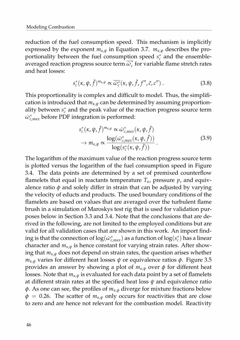
Modeling Combustion
reduction of the fuel consumption speed. This mechanism is implicitlyexpressed by the exponent mκ,ψ in Equation 3.7. mκ,ψ describes the pro-portionality between the fuel consumption speed s∗c and the ensemble-averaged reaction progress source term ω
∗c for variable flame stretch rates
and heat losses:
s∗c (κ, ψ, f )mκ,ψ ∝ ω∗c (κ, ψ, f , f ′′, c, c′′) . (3.8)
This proportionality is complex and difficult to model. Thus, the simplifi-cation is introduced that mκ,ψ can be determined by assuming proportion-ality between s∗c and the peak value of the reaction progress source termω∗c,max before PDF integration is performed:
s∗c (κ, ψ, f )mκ,ψ ∝ ω∗c,max(κ, ψ, f )
→ mκ,ψ ∝log(ω∗c,max(κ, ψ, f ))
log(s∗c (κ, ψ, f )).
(3.9)
The logarithm of the maximum value of the reaction progress source termis plotted versus the logarithm of the fuel consumption speed in Figure3.4. The data points are determined by a set of premixed counterflowflamelets that equal in reactants temperature Tu, pressure p, and equiv-alence ratio φ and solely differ in strain that can be adjusted by varyingthe velocity of educts and products. The used boundary conditions of theflamelets are based on values that are averaged over the turbulent flamebrush in a simulation of Maroskys test rig that is used for validation pur-poses below in Section 3.3 and 3.4. Note that the conclusions that are de-rived in the following, are not limited to the employed conditions but arevalid for all validation cases that are shown in this work. An import find-ing is that the connection of log(ω∗c,max) as a function of log(s∗c ) has a linearcharacter and mκ,ψ is hence constant for varying strain rates. After show-ing that mκ,ψ does not depend on strain rates, the question arises whethermκ,ψ varies for different heat losses ψ or equivalence ratios φ. Figure 3.5provides an answer by showing a plot of mκ,ψ over φ for different heatlosses. Note that mκ,ψ is evaluated for each data point by a set of flameletsat different strain rates at the specified heat loss ψ and equivalence ratioφ. As one can see, the profiles of mκ,ψ diverge for mixture fractions belowφ = 0.26. The scatter of mκ,ψ only occurs for reactivities that are closeto zero and are hence not relevant for the combustion model. Reactivity
46
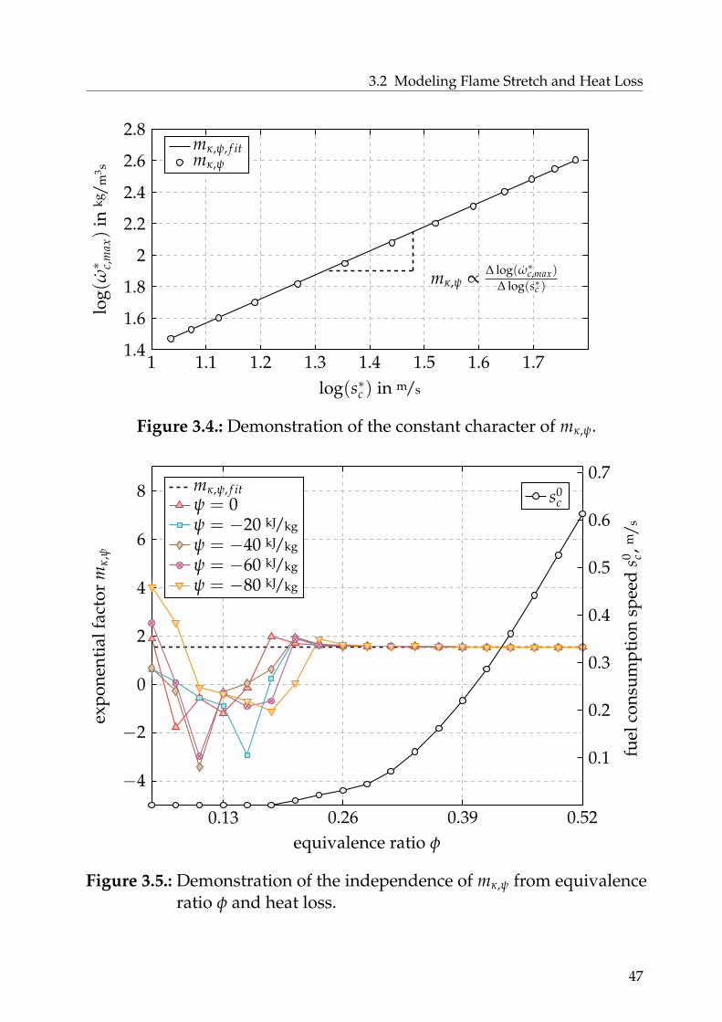
3.2 Modeling Flame Stretch and Heat Loss
1 1.1 1.2 1.3 1.4 1.5 1.6 1.71.4
1.6
1.8
2
2.2
2.4
2.6
2.8
mκ,ψ ∝ ∆ log(ω∗c,max)
∆ log(s∗c )
log(s∗c ) in m/s
log(
ω∗ c,
max)
inkg
/m3 s
mκ,ψ, f itmκ,ψ
Figure 3.4.: Demonstration of the constant character of mκ,ψ.
0.13 0.26 0.39 0.52
−4
−2
0
2
4
6
8
equivalence ratio φ
expo
nent
ialf
acto
rm
κ,ψ
mκ,ψ, f itψ = 0ψ = −20 kJ/kg
ψ = −40 kJ/kg
ψ = −60 kJ/kg
ψ = −80 kJ/kg
0.1
0.2
0.3
0.4
0.5
0.6
0.7
fuel
cons
umpt
ion
spee
ds0 c,
m/s
s0c
Figure 3.5.: Demonstration of the independence of mκ,ψ from equivalenceratio φ and heat loss.
47
Modeling Combustion
is indicated by the fuel consumption speed sc, which is plotted using asecond y-axis.
Based on the conclusions that are derived from Figure 3.4 and Figure 3.5,a constant value for the proportionality exponent mκ,ψ can be considered.The assumption of using a constant proportionality exponent mκ,ψ has agreat advantage, as a further tabulation strategy for mκ,ψ as a functionof mixture fraction f and heat loss ψ is not necessary. The proportional-ity exponent mκ,ψ is determined once at an arbitrary mixture fraction andheat loss (within the flammability limits) as the gradient of a fitted linearequation. The resulting flow of information for the described model isgiven in Figure 3.6. During run time, the code looks up unstretched, adi-abatic fuel consumption speeds s0
c as well as stretched, non-adiabatic fuelconsumption speeds s∗c . Significant heat losses and elevated flame stretchrates cause the fuel consumption speed s∗c to deviate from s0
c . This resultsin a change of the correction factor Γ that implicitly affects the reactionprogress source term and the shape of the turbulent flame brush. Differ-ences in comparison to the original FGM, which is depicted in Figure 3.1,are as follows:
• PDF integrated tables that provide mass fractions Ys, temperatureT and the reaction progress source term ω0
c are based on counter-flow flamelets at negligible stretch and adiabatic conditions insteadof freely propagating flamelets.
• Further tables are required that store the fuel consumption speeds s0c
and s∗c as well as the proportionality factor mκ,ψ. During run time, thecode looks up correction factors as a function of mixture fraction f ,stretch κ, and heat loss ψ.
The introduced FGM model extension requires to evaluate stretch andheat loss in premixed counterflow flamelets, which is discussed in thenext Section 3.2.1. In addition, the determination of heat loss in CFD isdiscussed in Section 3.2.2 and the determination of stretch in the scope ofRANS is discussed in Section 3.2.3.
48

3.2 Modeling Flame Stretch and Heat Loss
f
κstψ
f , κ, ψ s∗c(κ, ψ, f
)
Γ(s∗c , s0c)
s0c(
f)
additional manifold
computationalgrid
adiabatic premixed
Ys( f , c)T( f , c)
ω0c ( f , c)
PDFintegrated
Ys(c, c′′, f , f ′′)
T(c, c′′, f , f ′′)
ω0c (c, c′′, f , f ′′)
c, c′′, f , f ′′
CFD solver
viewer
unstretched,
tables
pre-
post-processing
counterflow flamelets
adiabatic premixedstretched, non-
counterflow flamelets
s0c( f )
tables
s∗c ( f )
mκ,ψ
ψ
Γ(κ, ψ, f )
stretch evaluation(Sec. 3.2.1)
heat loss evaluation(Sec. 3.2.1)
stretch
(Sec. 3.2.3)evaluation
heat loss
(Sec. 3.2.2)evaluation
solving
κ
f
ψ
κ
processing
Figure 3.6.: Simplified overview of FGM that considers stretch and heatloss.
3.2.1. Determination of Stretch and Heat Loss in Premixed CounterflowFlames
As discussed in Section 2.3.2, flame stretch consists of strain and curva-ture. Unfortunately, premixed counterflow flamelets can only be simu-lated at elevated strain rates as curvature is not achievable due to theone-dimensional character of the flame. Thus, the tabulation of flameletsat various flame stretch rates is not possible. As stated by Poinsot et al.[28, 67], strain and curvature have a similar impact on the physicochem-ical properties of the flame, at least for small flame stretch rates. Thishypotheses is exploited, as the tables for fuel consumption rates sc are
49

Modeling Combustion
parametrized with strain from the one-dimensional flamelet calculationsand looked up with flame stretch (strain + curvature) that is evaluatedin the context of RANS. Strain can be obtained from the one-dimensionalvelocity field using
κst = −∂ux
∂x, (3.10)
which is valid for incompressible flows due to the following relation:
0 =∂ux
∂x+
∂uy
∂y+
∂uz
∂z︸ ︷︷ ︸κst
. (3.11)
The velocity profile in a premixed counterflow flamelet is not linear overspace and strain differs for each location. Consequently, the location atwhich strain should be evaluated must be defined. Flame stretch altersthe flame velocity by changing the diffusive heat and species exchangebetween the flame front and the unburnt material. It is thus reasonableto determine strain at the interface between reactants and flame front.This position is evaluated by identifying the grid point that is locatedright before the flow accelerates due to the expansion of gas caused bythe density drop.
In order to determine the influence of heat loss, the manifolds must beparametrized by different levels of enthalpy. A non-adiabatic simulationwould usually indicate that there is a source term in the energy equationthat covers heat losses. Unfortunately, this would lead to several diffi-culties. For instance, the heat loss could not be defined but would resultfrom the solution. Hence, the flamelet simulations are performed at a setof predefined enthalpy levels. A reduced enthalpy corresponds to heatloss and is obtained by changing the reactants temperature. Further in-formation on the approach of employing flamelets at different enthalpylevels for non-adiabatic simulations is discussed by Fiorina et al. [68].
3.2.2. Modeling Heat Loss in the Context of CFD
Non-adiabatic effects are evaluated by a transport equation for energy. Asmentioned before, different forms of the energy equation exists. Equation
50

3.2 Modeling Flame Stretch and Heat Loss
2.11 is employed in the present work that transports the sum of chemicaland sensible enthalpy (denoted as h). This form has the advantage to beconservative during the combustion process. Changes in the chemically-bonded enthalpy are fully converted into sensible enthalpy. Furthermore,heat loss ψ is the distance of the non-adiabatic enthalpy h to the adiabaticenthalpy had:
ψ = h− had . (3.12)
Similar approaches can be found by Wetzel et al. [69] and by Frank etal. [70]. Adiabatic enthalpy needs to be determined as a function of mix-ture fraction. Enthalpy depends linearly on mixture fraction and can beevaluated using:
had = h1 f + h0(1− f ) . (3.13)
The indices 1 and 0 corresponds to a mixture fraction of unity (fuel) andzero (oxidizer).
3.2.3. Modeling Flame Stretch Rates in the Context of RANS
The fundamentals of flame stretch can be found in Section 2.3.2 in whichthe following equation is stated:
〈κst〉 = ∇ · u− 〈n⊗ n〉 : ∇u︸ ︷︷ ︸κst
+ 〈sd∇ · n〉︸ ︷︷ ︸κcurv
. (3.14)
Flame stretch is a continuous field and differs for each position of theflame front. Hence, the discrete flame surface that is located within acell has a variety of different flame stretch rates. The models that areintroduced in the following, determine cell-averaged flame stretch rates,which is indicated by 〈 〉. Equation 3.14 shows the two parts flame stretchconsists of. In the context of RANS, only the Favre-averaged velocity isknown. Thus, it is reasonable to divide the strain term in order to modelthe first two conditional moments of velocity separately:
〈κst〉 = ∇ · u− 〈n⊗ n〉 : ∇u︸ ︷︷ ︸κst
+ 〈∇ · u′′ − 〈n⊗ n〉 : ∇u′′〉︸ ︷︷ ︸κ′′st
+ 〈sd∇ · n〉︸ ︷︷ ︸κcurv
.
(3.15)
51

Modeling Combustion
In the next three sections, the modeling of each term is presented.
3.2.3.1. Modeling Mean Flame Stretch Rates
The mean flame stretch rate
〈κst〉 = ∇ · u− 〈n⊗ n〉 : ∇u (3.16)
in index notation reads
〈κst〉 =(δij −
⟨ninj
⟩) ∂ui
∂xj. (3.17)
The orientation factors ninj are unknown and require modeling. Veynanteet al. [71,72] observed the following relationship between orientation fac-tors and Reynolds stresses in a two-dimensional, V-shaped flame4:
⟨ninj=i
⟩=
∑k 6=i u′′k2
4kand
⟨ninj 6=i
⟩=
u′′i u′′j2k
. (3.18)
The turbulent kinetic energy k can be retrieved from the turbulencemodel. Furthermore, the Reynolds stresses are estimated using the ap-proximation by Boussinesq (cf. Equation 2.28).
3.2.3.2. Modeling Turbulent Flame Stretch Rates
〈κ′′st〉 = 〈∇ · u′′ − n⊗ n : ∇u′′〉 (3.19)
Strain due to turbulent fluctuations is determined using the IntermittentTurbulence Net Flame Stretch (ITNFS) model proposed by Meneveau andPoinsot [74] on the basis of chemical and turbulent time and length scales:
〈κ′′st〉 = I(
u′
sl,
lint
l f
)ε
k. (3.20)
The function I is derived from a DNS in which the interaction of counter-rotating pairs with flame fronts is analyzed. An advantage over other
4 Note that this model is also valid in three dimensions as demonstrated in a DNS by Katragadda et al.[73].
52
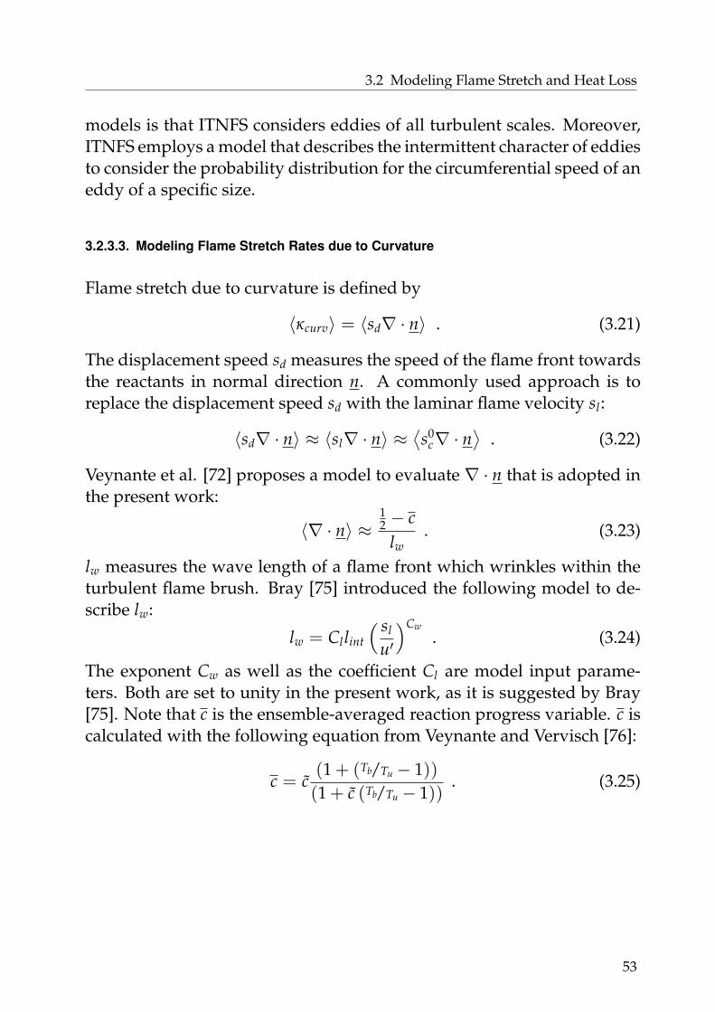
3.2 Modeling Flame Stretch and Heat Loss
models is that ITNFS considers eddies of all turbulent scales. Moreover,ITNFS employs a model that describes the intermittent character of eddiesto consider the probability distribution for the circumferential speed of aneddy of a specific size.
3.2.3.3. Modeling Flame Stretch Rates due to Curvature
Flame stretch due to curvature is defined by
〈κcurv〉 = 〈sd∇ · n〉 . (3.21)
The displacement speed sd measures the speed of the flame front towardsthe reactants in normal direction n. A commonly used approach is toreplace the displacement speed sd with the laminar flame velocity sl:
〈sd∇ · n〉 ≈ 〈sl∇ · n〉 ≈⟨s0
c∇ · n⟩
. (3.22)
Veynante et al. [72] proposes a model to evaluate ∇ · n that is adopted inthe present work:
〈∇ · n〉 ≈12 − c
lw. (3.23)
lw measures the wave length of a flame front which wrinkles within theturbulent flame brush. Bray [75] introduced the following model to de-scribe lw:
lw = Cllint
( sl
u′)Cw
. (3.24)
The exponent Cw as well as the coefficient Cl are model input parame-ters. Both are set to unity in the present work, as it is suggested by Bray[75]. Note that c is the ensemble-averaged reaction progress variable. c iscalculated with the following equation from Veynante and Vervisch [76]:
c = c(1 + (Tb/Tu − 1))(1 + c (Tb/Tu − 1))
. (3.25)
53

Modeling Combustion
100.0
0.0
0.75 fburner
fburner
u in ms
section plane
air
flamelet
flame brush
air OH∗-data
ORZ
IRZ
f
cooled walls
for contour plots
d bur
ner
4d b
urne
r
0.12 dburner
0.3 dburner
gas/
1.7 dburner
1.2
d bur
ner
secondary
2d b
urne
r
5.3 dburner
h241
l6352.635
Figure 3.7.: Illustration of Marosky’s [58] validation case.
3.3. Application and Validation
The proposed combustion modeling strategy is implemented in FLUENT
[77] by extending the functionality of the original FGM infrastructure.Moreover, a software is developed that automatically generates the tableson the basis of premixed counterflow flamelets. Details to the softwareimplementation can be found in Appendix A. Note that the software in-cludes both the combustion and the CO modeling that is introduced inthe next chapter. Computational overhead caused by the model exten-sion is negligibly small. The introduced modeling approach is appliedto an atmospheric single-burner test rig from Marosky [58], which is il-lustrated in Figure 3.7. A mixture of air and natural gas is preheated to673.15 K and enters the combustion chamber through the A2EV5 burner.The swirling flow breaks down in the combustion chamber and providesa stagnation point near the burner exit at which the combustion stabilizes.3 % of the total amount of preheated air flows through a perforated frontplate into the combustion chamber near to the burner exit. Fuel mass flowis adjusted to achieve a global equivalence ratio of φ = 0.5. The valida-tion case features considerable heat loss over the cooled walls. Figure 3.7
5 Details regarding the A2EV burner can be found in Sangl [78] and Mayer [79].
54

3.3 Application and Validation
ORZ
IRZ
100.0
0.0
0.75 fburner
fburner
u in m/s
velocity
fraction fmixture
Figure 3.8.: Distributions of velocity (upper half) and mixture fraction(lower half) of Marosky’s [58] validation case.
shows an area that is marked by white stripes in which OH∗-emissivitydata is available.
The domain is discretized by employing a block structured grid. Amesh independence analysis in a way proposed by Ferziger and Peric[80] is conducted in order to guarantee a mesh independent solution. InMarosky’s experiment, the outer shell of the wall is cooled by impingingair. As the CFD simulation does not include the environment, an energeticboundary condition needs to be modeled in order to cover the significantheat losses. For this purpose, a thermal boundary condition is used thatcalculates the heat flux on the basis of the heat transfer coefficient α andthe difference between wall temperature and the ambient temperature.Unfortunately, the heat transfer coefficient α is unknown and needs to beestimated. For this purpose, the highest experimental wall temperatureis estimated by the brightest color of the glowing steel that has been ex-perimentally observed. Moreover, α is automatically iterated in the sim-ulation until the wall temperature in the simulations meet the estimated
55
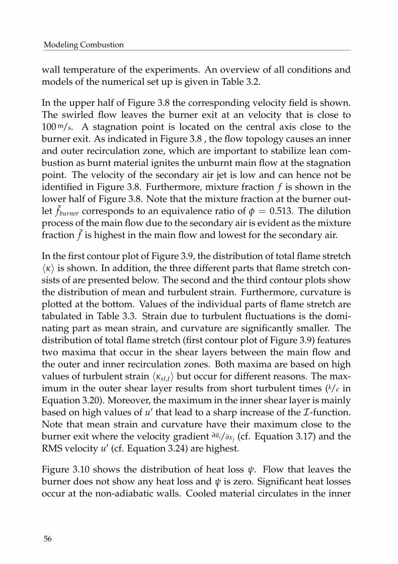
Modeling Combustion
wall temperature of the experiments. An overview of all conditions andmodels of the numerical set up is given in Table 3.2.
In the upper half of Figure 3.8 the corresponding velocity field is shown.The swirled flow leaves the burner exit at an velocity that is close to100 m/s. A stagnation point is located on the central axis close to theburner exit. As indicated in Figure 3.8 , the flow topology causes an innerand outer recirculation zone, which are important to stabilize lean com-bustion as burnt material ignites the unburnt main flow at the stagnationpoint. The velocity of the secondary air jet is low and can hence not beidentified in Figure 3.8. Furthermore, mixture fraction f is shown in thelower half of Figure 3.8. Note that the mixture fraction at the burner out-let fburner corresponds to an equivalence ratio of φ = 0.513. The dilutionprocess of the main flow due to the secondary air is evident as the mixturefraction f is highest in the main flow and lowest for the secondary air.
In the first contour plot of Figure 3.9, the distribution of total flame stretch〈κ〉 is shown. In addition, the three different parts that flame stretch con-sists of are presented below. The second and the third contour plots showthe distribution of mean and turbulent strain. Furthermore, curvature isplotted at the bottom. Values of the individual parts of flame stretch aretabulated in Table 3.3. Strain due to turbulent fluctuations is the domi-nating part as mean strain, and curvature are significantly smaller. Thedistribution of total flame stretch (first contour plot of Figure 3.9) featurestwo maxima that occur in the shear layers between the main flow andthe outer and inner recirculation zones. Both maxima are based on highvalues of turbulent strain 〈κst,t〉 but occur for different reasons. The max-imum in the outer shear layer results from short turbulent times (k/ε inEquation 3.20). Moreover, the maximum in the inner shear layer is mainlybased on high values of u′ that lead to a sharp increase of the I-function.Note that mean strain and curvature have their maximum close to theburner exit where the velocity gradient ∂ui/∂xj (cf. Equation 3.17) and theRMS velocity u′ (cf. Equation 3.24) are highest.
Figure 3.10 shows the distribution of heat loss ψ. Flow that leaves theburner does not show any heat loss and ψ is zero. Significant heat lossesoccur at the non-adiabatic walls. Cooled material circulates in the inner
56

3.3 Application and Validation
Table 3.2.: Summary of the numerical setup for Marosky’s [58] test rig.
boundary conditions:
T∞ 300 K
Tu 673.15 K
αwall 50 W/m2K
m0 (air) 400 g/s
m0,sec (air) 3 % of m0
φ 0.5
CFD:
CFD software FLUENT v18.0 [77]
turbulence model k-ω SST
Sct 0.7
mesh type hexahedral (block structured)
mesh size (without burner) 1.7e6 cells
flamelet generation:
kinetic GRI 3.0 [37]
discrete points of c/ f /ψ/κ 232/21/21/≈19
mκ,ψ 1.49
57
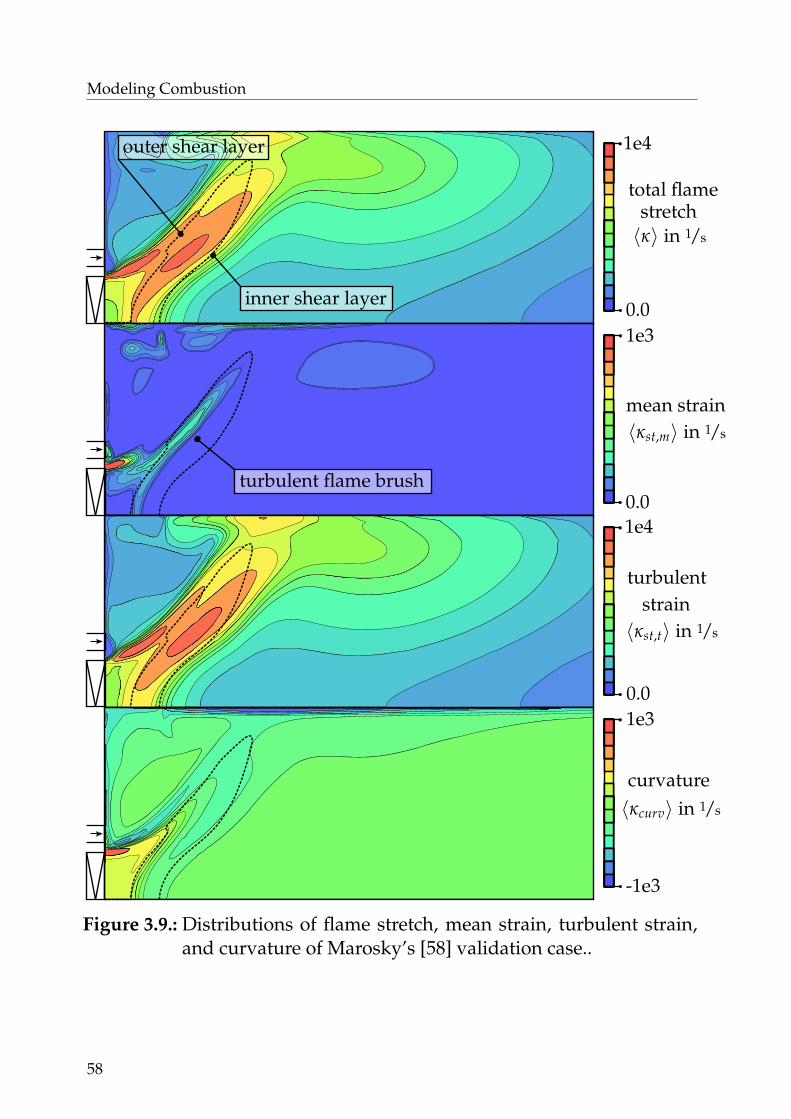
Modeling Combustion
turbulent flame brush
inner shear layer
outer shear layer
1e4
0.0
-1e3
1e3
strain
〈κcurv〉 in 1/s
curvature
1e4
0.0
0.0
1e3
total flame
〈κst,m〉 in 1/s
mean strain
〈κ〉 in 1/s
〈κst,t〉 in 1/s
turbulent
stretch
Figure 3.9.: Distributions of flame stretch, mean strain, turbulent strain,and curvature of Marosky’s [58] validation case..
58

3.3 Application and Validation
Table 3.3.: Strain and curvature averaged over the turbulent flame brush.
total flame stretch 〈κ〉t f b 7603 1/s
mean strain 〈κst,m〉t f b 54 1/s
turbulent strain 〈κst,t〉t f b 7690 1/s
curvature 〈κcurv〉t f b −141 1/s
0.0
−400.0
0.75 fburner
fburner
heat loss
fraction fmixture
ψ in kJ/kg
Figure 3.10.: Distribution of heat loss ψ of Marosky’s [58] validation case.
and outer recirculation zone. The outer recirculation zone shows signifi-cantly higher heat losses than the inner recirculation zone as the velocityin the outer recirculation zone is low and the residence time is hence in-creased. The high heat losses in the outer recirculation zone lead to lowenthalpies in the outer shear layer causing a significant reduction of reac-tivity in this region. Figure 3.11 shows the distributions of reference fuelconsumption speed s0
c and the non-adiabatic, strained fuel consumptionspeed s∗c . s0
c is solely a function of the mixture fraction. It approacheszero for pure air at the secondary air inlet and reaches its maximum at theburner outlet where the mixture is not yet diluted by the secondary air in-jector. Flame stretch and heat loss have a substantial impact on the flamespeed as shown in the lower half of Figure 3.11. The fuel consumptionspeed approaches zero in the outer recirculation zone due to the substan-tial heat loss in this region. Moreover, high flame stretch rates occur in theinner shear layer causing a local minimum of the fuel consumption speeds∗c .
59
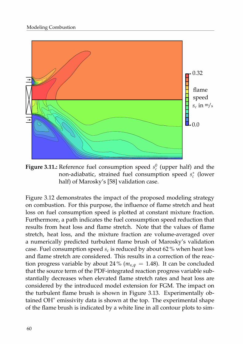
Modeling Combustion
0.0
0.32
sc in m/s
speedflame
Figure 3.11.: Reference fuel consumption speed s0c (upper half) and the
non-adiabatic, strained fuel consumption speed s∗c (lowerhalf) of Marosky’s [58] validation case.
Figure 3.12 demonstrates the impact of the proposed modeling strategyon combustion. For this purpose, the influence of flame stretch and heatloss on fuel consumption speed is plotted at constant mixture fraction.Furthermore, a path indicates the fuel consumption speed reduction thatresults from heat loss and flame stretch. Note that the values of flamestretch, heat loss, and the mixture fraction are volume-averaged overa numerically predicted turbulent flame brush of Marosky’s validationcase. Fuel consumption speed sc is reduced by about 62 % when heat lossand flame stretch are considered. This results in a correction of the reac-tion progress variable by about 24 % (mκ,ψ = 1.48). It can be concludedthat the source term of the PDF-integrated reaction progress variable sub-stantially decreases when elevated flame stretch rates and heat loss areconsidered by the introduced model extension for FGM. The impact onthe turbulent flame brush is shown in Figure 3.13. Experimentally ob-tained OH∗ emissivity data is shown at the top. The experimental shapeof the flame brush is indicated by a white line in all contour plots to sim-
60

3.3 Application and Validation
1e3
4.03.0
2.01.0
0.0
1e4
0.0
0.40.8
1.2
0.1
0.2
0.3
0.4
0.5
0
10
20
30
40
50
60
70
0
heat loss ψ in kJ/kg strain κ stin
1/s
flam
esp
eed
s∗ cin
m/s
flam
esp
eed
s0 cin
cm s
s0c = 0.58 m/s
s∗c = 0.22 m/s
fburnermixture fraction f
0.6
Figure 3.12.: Demonstration of the influence of flame stretch and heatloss on flame speed. The corresponding values are volume-averaged over a numerically predicted turbulent flamebrush of Marosky’s validation case (cf. Table 3.2 and 3.3).
plify comparison. In the top left corner, the distribution of the unmodi-fied reaction progress source term (Γ = 1.0) is shown. The numericallypredicted heat release distribution of the original FGM deviates signif-icantly from the experimental flame shape: Reactivity is overestimatedin the outer shear layer, the flame brush thickness is too thin, and theflame stabilizes near the burner outlet. No major improvement can beachieved when solely heat loss is taken into account as shown in the topright corner. It can be concluded that the prediction of the heat releasedistribution of Marosky’s [58] validation case is not significantly gettingimproved by considering heat loss only. The contour plot in the bottomleft corner shows the heat release distribution when solely flame stretch
61
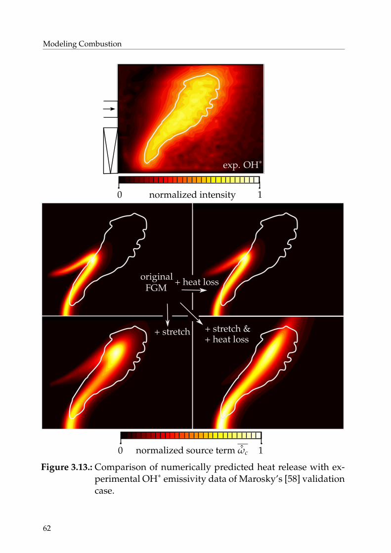
Modeling Combustion
OH*-emissivitymeasurement
+ stretch &
1 1s
0 1s
Γ(κ = 0.0, ψ 6= 0.0)
Γ(κ 6= 0.0, ψ 6= 0.0)
Γ(κ = 0.0, ψ = 0.0)
Γ(κ 6= 0.0, ψ = 0.0)
exp. shape
+ heat loss
ˆωc+ heat loss
+ stretch
Γ(κ 6= 0.0, ψ = 0.0)
exp. OH∗
Γ(κ 6= 0.0, ψ 6= 0.0)
original
Γ(κ = 0.0, ψ 6= 0.0)
+ stretch &+ heat loss
+ stretch
FGM
turbulent flame brush
inner shear layer
outer shear layer
10 000.0
0.0
−1000.0
1000.0
strain
〈κcurv〉 in 1s
curvature
1000.0
0.0
0.0
1000.0
kappa
〈κst,m〉 in 1s
mean strain
〈κ〉 in 1s
〈κst,t〉 in 1s
turbulent
+ heat loss
10
normalized intensity 10
normalized source term ˆωc
Figure 3.13.: Comparison of numerically predicted heat release with ex-perimental OH∗ emissivity data of Marosky’s [58] validationcase.
62

3.4 Model Comparison
is considered. Flame stretch has a major impact and leads to a substantialimprovement regarding position and shape of the turbulent flame brush.Nevertheless, the outer shear layer still exhibits minor heat release thatis not in accordance with the experiments. The final model is shown inthe bottom right corner. Reaction rates in the outer shear layer disappearsand the numerically predicted turbulent flame brush is in good agreementwith the experimental shape.
3.4. Model Comparison
Finally, a qualitative comparison of standard combustion models is per-formed and benchmarked using the experimental data by Marosky [58].A short introduction to the models was provided in Section 2.3.4. Fur-ther information regarding the model implementations can be found inANSYS [81].
The heat release prediction by EDM is shown in the lop left corner ofFigure 3.14. As stated by Poinsot and Veynante [28], combustion mod-els that are based on the EBU theory often overestimate the reaction rateswhen the characteristic turbulent time scale k/ε becomes large. This crit-icism is justified by the incorrectly predicted heat release distribution re-sulting from the use of EDM. Combustion is drastically overestimated inthe shear layer to the outer recirculation zone. High strain rates occurin this region leading to significant damping of the reaction rates that isnot considered by EDM. The strategy of adding a kinetic limitation to thespecies source terms in EDM is presented in the top right corner of Figure3.14. No significant improvement is achieved as the flame brush becomeslonger but no quenching of the outer shear layer occurs. Note that theEDM/FR model formulation implicitly accounts for heat loss since thedecreased temperature influences the finite rate that is calculated by theArrhenius law. A similar issue occurs by employing the TFC closure byZimont et al. [51,52] as shown in the middle left. Furthermore, the middleright of Figure 3.14 shows the TFC model with a flame stretch correctionthat was proposed by Zimont et al. [52]. A substantial improvement byusing the flame stretch correction is evident. The flame length fits the ex-perimental shape but combustion still takes place in the shear layer that
63
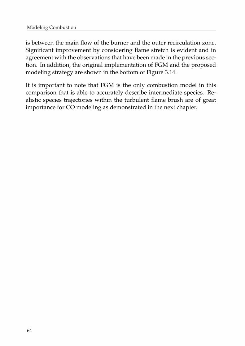
Modeling Combustion
is between the main flow of the burner and the outer recirculation zone.Significant improvement by considering flame stretch is evident and inagreement with the observations that have been made in the previous sec-tion. In addition, the original implementation of FGM and the proposedmodeling strategy are shown in the bottom of Figure 3.14.
It is important to note that FGM is the only combustion model in thiscomparison that is able to accurately describe intermediate species. Re-alistic species trajectories within the turbulent flame brush are of greatimportance for CO modeling as demonstrated in the next chapter.
64
3.4 Model Comparison
10
EDM/FREDM
TFC
10 normalized source term ˆωc
normalized heat release ˆωT
stretched,non-adiabatic
originalFGM
stretchedTFC
FGM
Figure 3.14.: Qualitative comparison of different standard combustionmodels.
65


4 Modeling CO
Flamelet-based approaches are able to accurately predict heat release dis-tributions in cold conditions in a way that was demonstrated in Chapter3. The question arises whether flamelets are also capable of describingCO emissions. As mentioned before, the typical thickness of a flameletis usually several orders of magnitude smaller than the usual length ofgas turbine combustors. The existence of CO emissions in the exhaust gasindicates that the CO burnout time is longer than the residence time inthe combustion chamber. Predicting global CO with FGM would hencerequire flamelets to fluctuate through the whole gas turbine. This is un-likely as the turbulent flame brush stabilizes at the stagnation point thatis provided by the vortex breakdown near the burner exit. It can be con-cluded that the successful modeling of CO emissions requires to performa paradigm shift to describe the burnout region in which the flamelet as-sumption is not valid anymore. For this purpose, an approach that iscapable of modeling the transition from flamelets to the kinetically lim-ited burnout is presented in this chapter. In the first section, the basicidea of dividing the domain into several subregions is presented. Eachsub region requires a specific modeling strategy that is covered by theSections 4.2, 4.3, 4.4, and 4.5. Moreover, Section 4.6 shows the applica-tion of the proposed modeling strategy. Three different validation casesare employed in order to assess the model performance. In addition, themodel is applied to an advanced combustor concept.
67

Modeling CO
pre-flame in-flame
YCO, f gm
c = 0 c = 1
Lines SurfacesFont
YCO
post-flame
decoupling
YCO, model
sec. air
quenched
quenching traveleddistance x
τt τox,CO τcr,OH
Figure 4.1.: Illustration of the domain partitioning that identifies thezones of different CO modeling.
4.1. Separating Time Scales
In order to describe CO separately from the combustion model, an addi-tional transport equation is required:
∂ρYCO
∂t+
∂ρuiYCO
∂xi=
∂
∂xi
(µt
Sct
∂YCO
∂xi
)+ ωCO . (4.1)
The strategy for closing this equation is based on the spatial division intomultiple zones in a way that is illustrated in Figure 4.1. A Lagrangianobserver is shown that travels on a trajectory through a combustor and
68

4.1 Separating Time Scales
passes several regions. The observer’s position determines the employedsubmodel for CO. In the lower half of Figure 4.1, a qualitative profile ofCO as a function of the Lagrangian observer’s traveled distance is shown.The first profile ( ) represents CO predicted by the combustion model.As the Favre-averaged reaction progress c reaches unity, the probabilityof flamelets is zero and CO is by definition in its equilibrium state. Asecond profile ( ) shows the prediction by the CO model that is intro-duced in the present chapter. CO is described by the combustion modelonly up to a certain point, which is denoted as the decoupling event. Thedecoupling event marks the point at which the burnout chemistry can-not be described by flamelets anymore. After CO left the flamelet-basedspecies trajectories, CO oxidation becomes slower due to the absence ofthe flamelet’s radical pool. Moreover, the post-flame model presented inthis work looses its validity in situation in which the equivalence ratio issignificantly decreased. In summary, four different regions of differentmodeling are defined:
• pre-flame zone ( ): The source terms for CO are negligibly smallbefore the chain-branching chemistry starts. Thereby, this zone doesnot require modeling.
• in-flame zone ( ): This region is dominated by the time scales ofturbulent mixing. Combustion chemistry is fast and can be describedby flamelets. Hence, CO is derived from the combustion model in theway that is presented in Section 4.2.
• post-flame zone ( ): Behind the turbulent flame brush, super-equilibrium species may occur like elevated CO. In this region,chemical time scales are usually small as the in-flame radical poolis not available anymore. The modeling approach for the post-flameregion is introduced in Section 4.3. Furthermore, Section 4.4 presentsa model for predicting the transition from the in- to the post-flamezone.
• quenched zone ( ): In the potential situation of lean quenching, theequivalence ratio is low and the chemical rates are negligibly small.As argued in Section 4.5, this region is dominated by the creationtime scale of OH.
69
Modeling CO
4.2. Modeling In-Flame CO
Within the turbulent flame brush, CO is tabulated on the basis of PDF-integrated profiles of flamelets. The previously introduced combustionmodel modifies the reaction progress source term in order to take flamestretch and heat loss into account. The question arises whether the tabu-lated CO profiles also need correction in terms of flame stretch and heatloss. Figure 4.2 gives an answer by showing CO profiles at various flamestretch rates. Flame stretch alters the molecular diffusion of heat andspecies within the flamelet. Adding flame stretch and heat loss as furtherdimensions to the tabulation process would significantly increase the nu-merical effort. A reasonable alternative is thus to tabulate the unstretched,adiabatic mass fraction of CO and to model the influence of flame stretchand heat loss. Note that this approach is similar to the concept of the cor-rection factor Γκ,ψ that was introduced in the previous chapter in Equation3.5. The tabulation of CO on the basis of freely-propagating flamelets (un-stretched and adiabatic) reads
Y0CO =
∫∫Y0
CO (c, f )P(c, c, c′′)P( f , f , f ′′)dcd f . (4.2)
The question arises whether the correction factor Γκ,ψ can be employed tomodify Y0
CO in the same way it is used to correct ω0c in Equation 3.5. In the
proposed combustion modeling strategy, the correction factor Γκ,ψ wasmodeled in Equation 3.7 without differentiating whether the reduction infuel consumption speed sc is due to flame stretch κ or heat loss ψ. An in-terpretation of this assumption is that sc and the reaction progress sourceterm ωc are both quantities describing reactivity. Hence, changing sc hasa direct effect on the reaction progress source term ωc, regardless whetherthe reduction in reactivity is based on flame stretch or heat loss. Unfor-tunately, this assumption does not apply for the connection between fuelconsumption speed sc and CO. It can be shown that flame stretch κ of-ten has a significant influence on CO while the impact of heat loss ψ ismoderate. Thus, flame stretch and heat loss need to be considered inde-pendently from each other by introducing two isolated correction factors:
Y∗CO = Γψ,COΓκ,CO
∫∫Y0
CO (c, f )P(c, c, c′′)P( f , f , f ′′)dcd f . (4.3)
70

4.2 Modeling In-Flame CO
0e0
5e−3
1e−2
1.5e−2 Tu = 573 Kp = 1 barκst=527 1/s
κst=1000 1/s
κst=1482 1/s
κst=1963 1/s
κst=2695 1/s
κst=3677 1/s
0e0
2e−3
4e−3
6e−3
mas
sfr
acti
onof
CO
Y CO Tu = 570 K
p = 15 barκst=489 1/s
κst=1185 1/s
κst=1910 1/s
κst=2634 1/s
κst=3377 1/s
κst=4657 1/s
0 0.1 0.2 0.3 0.4 0.5 0.6 0.7 0.8 0.9 10e0
2e−3
4e−3
6e−3
8e−3
reaction progress c
Tu = 674 Kp = 30 barκst=417 1/s
κst=2608 1/s
κst=4865 1/s
κst=7250 1/s
κst=9659 1/s
Figure 4.2.: Flame stretch dependency of CO demonstrated at three pres-sure levels (premixed counterflow flamelets at φ = 0.5, andTu = 573.15 K calculated using GRI 3.0 [37] and CANTERA
[34]).
71

Modeling CO
1.6 1.7 1.8 1.9 23.2
3.4
3.6
3.8
mκ,CO ∝∆ log(Y∗CO,max)
∆ log(sc∗ )
log(s∗c ) in m/s
log(
Y∗ C
O,m
ax)
inkg
/kg
1.6 1.7 1.8 1.9 2
mψ,CO ∝∆ log(Y∗CO,max)
∆ log(sc∗ )
log(s∗c ) in m/s
variation of stretchvariation of heat loss
Figure 4.3.: Demonstration of the constant character of the proportional-ity exponents mκ,CO and mψ,CO.
Furthermore, the correction factors read
Γψ,CO(κ0, ψ, f
)=
(s∗c(κ0, ψ, f
)
s0c(
f)
)mψ,CO
(4.4)
and Γκ,CO(κ, ψ0, f
)=
(s∗c(κ, ψ0, f
)
s0c(
f)
)mκ,CO
. (4.5)
Both relations are analytically correct if
s∗c(κ0, ψ, f
)mψ,CO ∼ Y∗CO
(κ0, ψ, f , c
)(4.6)
and s∗c(κ, ψ0, f
)mκ,CO ∼ Y∗CO
(κ, ψ0, f , c
)(4.7)
are valid. Direct modeling of these relations is difficult. Hence, the as-sumption is introduced that the proportionality between the peak valueof CO and the corresponding flame speed does not change due to PDFintegration. Note that this assumption was also used in the Equations 3.8and 3.9.
s∗c(κ0, ψ, f
)mψ,CO ∼ Y∗CO,max(κ0, ψ, f
)(4.8)
and s∗c(κ, ψ0, f
)mκ,CO ∼ Y∗CO,max(κ, ψ0, f
). (4.9)
72
4.3 Modeling Post-Flame CO
Finally, the proportionality exponents read
mψ,CO ∼log(Y∗CO,max
(κ0, ψ, f
))
log(s∗c(κ0, ψ, f
)) (4.10)
and mκ,CO ∼log(Y∗CO,max
(κ, ψ0, f
))
log(s∗c(κ, ψ0, f
)) . (4.11)
Both proportionality exponents can be interpreted as the gradients of afunctional correlation between log(YCO,max) and log(sc) as plotted in Fig-ure 4.3. The data points are determined by a set of premixed counterflowflamelets that equal in reactants temperature Tu, pressure p, and equiva-lence ratio φ and solely differ in strain (left hand side) or in heat loss (righthand side). Note that the used boundary conditions of the flamelets arebased on values that are averaged over the turbulent flame brush of avalidation case that will be introduced in Section 4.6.1 (cf. Table 4.1). Theimport conclusion of Figure 4.3 is that the connection of log(Y∗CO,max) asa function of log(s∗c ) has a linear character and mκ,CO as well as mψ,CO ishence constant for varying strain rates or heat losses. Due to the linearproportionalities, the exponents can be evaluated as the gradient of a fit-ted linear equation.
4.3. Modeling Post-Flame CO
As mentioned above, flamelets cannot be used to describe chemistry be-hind the turbulent flame brush. As shown in the following, the employ-ment of detailed chemistry is not necessarily needed due to the simplicityof CO burnout chemistry. The burnout of CO can be described using asingle reaction equation as mentioned by Turns [82]:
CO + OH −−→ CO2 + H . (4.12)
Reaction rates that are obtained from a zero-dimensional reactor simula-tion are shown in Figure 4.4 at three different constant pressure conditionsfor an equivalence ratio of φ = 0.3. Note that the reaction analysis is re-peated for an equivalence ratio of φ = 0.5 in the Appendix B. Note thatonly the late burnout is plotted. As one can see, CO + OH → CO2 + H
73

Modeling CO
0 1 2 3 4 5 6 7 8 9 10 11 12 13 14 15
1e−5
1e−3
1e−1
1e1
Tu = 573 K, p = 1 barr26/27: CO + OH <=> CO2 + Hr24: CO + O (+M) <=> CO2 (+M)r30: HCO + O2 <=> CO + HO2r28: CO + HO2 <=> CO2 + OH
0 5 10 15 20 25 30 35 40 45 50 55 601e−7
1e−5
1e−3
1e−1
1e1
rate
rin
mol/m
3 s
Tu = 570 K, p = 15 bar
0 1 2 3 4 5 6 7 8 9 10 11 121e−4
1e−3
1e−2
1e−1
1e0
1e1
1e2
time t in ms
Tu = 674 K, p = 30 bar
Figure 4.4.: Four most relevant CO reactions in the late burnout (constantpressure reactor at φ = 0.3, calculated using GALWAY 1.3 [38]and CANTERA [34]).
74

4.3 Modeling Post-Flame CO
( ) is always about two orders of magnitude greater than the secondstrongest reaction ( ). Using Equation 4.12 to close ωCO requires knowl-edge of the concentration of CO and OH as well as the non-adiabatictemperature. Temperature and the concentration of CO are known fromtheir corresponding transport equations. OH is unknown and need to bemodeled. The use of a kinetic mechanism to evaluate OH would requireto transport all participating species, leading to a tremendous increasein computational effort. Fortunately, OH kinetic mechanisms are not re-quired, as discussed in the following.
It is frequently reported in literature that OH is in equilibrium during theburnout of CO. For instances, Connors et al. [83] assumes OH to be inequilibrium for the development of a semi-empirical model to globallypredict CO emissions in gas turbines. Using this assumption, the post-flame source term of CO can be evaluated using
− d [CO]
dt= karr, f or (T) [CO] [OH]eq . (4.13)
In the present work, the equilibrium of OH is determined using GAL-WAY 1.3 [38] kinetics. Furthermore, karr, f or is calculated using Arrheniusparameters from Joshi and Wang [84] that are also included in GALWAY
1.3.
The model simplifications are further discussed and validated in the fol-lowing. Flagan and Seinfeld [85] compared time scales of different ap-proaches for treating OH and karr, f or. For this purpose, a characteristictime scale for the burnout of CO is defined:
τCO =[CO]
karr, f or[CO][OH]=
1karr, f or[OH]
. (4.14)
τCO as a function of φ is plotted in Figure 4.5. Several models are reprintedand compared to the proposed post-flame model ( ). The second model( ) equals the approach in this work, as OH is assumed to be in equilib-rium and karr, f or is based on shock tube experiments. Note that deviationsbetween the first two approaches ( and ) may be related to differ-ent Arrhenius parameters for the evaluation of karr, f or (cf. Equation 2.9).Moreover, the third profile ( ) represents a model by Fristrom and West-
75
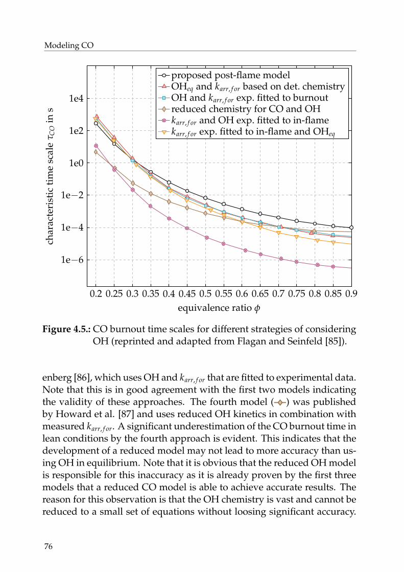
Modeling CO
0.2 0.25 0.3 0.35 0.4 0.45 0.5 0.55 0.6 0.65 0.7 0.75 0.8 0.85 0.9
1e−6
1e−4
1e−2
1e0
1e2
1e4
equivalence ratio φ
char
acte
rist
icti
me
scal
eτ C
Oin
s
proposed post-flame modelOHeq and karr, f or based on det. chemistryOH and karr, f or exp. fitted to burnoutreduced chemistry for CO and OHkarr, f or and OH exp. fitted to in-flamekarr, f or exp. fitted to in-flame and OHeq
Figure 4.5.: CO burnout time scales for different strategies of consideringOH (reprinted and adapted from Flagan and Seinfeld [85]).
enberg [86], which uses OH and karr, f or that are fitted to experimental data.Note that this is in good agreement with the first two models indicatingthe validity of these approaches. The fourth model ( ) was publishedby Howard et al. [87] and uses reduced OH kinetics in combination withmeasured karr, f or. A significant underestimation of the CO burnout time inlean conditions by the fourth approach is evident. This indicates that thedevelopment of a reduced model may not lead to more accuracy than us-ing OH in equilibrium. Note that it is obvious that the reduced OH modelis responsible for this inaccuracy as it is already proven by the first threemodels that a reduced CO model is able to achieve accurate results. Thereason for this observation is that the OH chemistry is vast and cannot bereduced to a small set of equations without loosing significant accuracy.
76
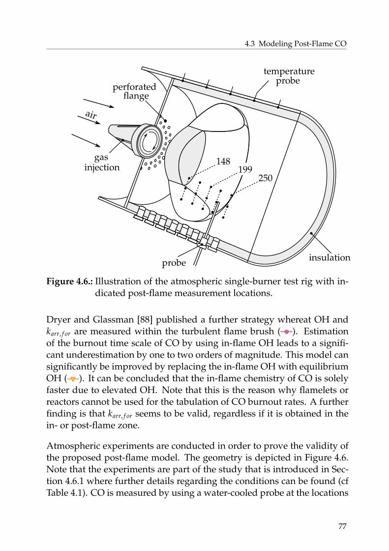
4.3 Modeling Post-Flame CO
perforatedflange
insulation
gasinjection
air
probe
temperatureprobe
148199
250
Figure 4.6.: Illustration of the atmospheric single-burner test rig with in-dicated post-flame measurement locations.
Dryer and Glassman [88] published a further strategy whereat OH andkarr, f or are measured within the turbulent flame brush ( ). Estimationof the burnout time scale of CO by using in-flame OH leads to a signifi-cant underestimation by one to two orders of magnitude. This model cansignificantly be improved by replacing the in-flame OH with equilibriumOH ( ). It can be concluded that the in-flame chemistry of CO is solelyfaster due to elevated OH. Note that this is the reason why flamelets orreactors cannot be used for the tabulation of CO burnout rates. A furtherfinding is that karr, f or seems to be valid, regardless if it is obtained in thein- or post-flame zone.
Atmospheric experiments are conducted in order to prove the validity ofthe proposed post-flame model. The geometry is depicted in Figure 4.6.Note that the experiments are part of the study that is introduced in Sec-tion 4.6.1 where further details regarding the conditions can be found (cfTable 4.1). CO is measured by using a water-cooled probe at the locations
77

Modeling CO
148 173.5 199 224.5 250−1
−0.8
−0.6
−0.4
−0.2
0
distance from front plate x in mm
ς CO
inkm
ol/m
3 s
Tad = 1602 K - derived from exp.Tad = 1602 K - post-flame modelTad = 1553 K - derived from exp.Tad = 1553 K - post-flame modelTad = 1553 K - reactor modelTad = 1553 K - flamelet model
Figure 4.7.: Comparison of experimental with modeled source terms ofCO.
that are indicated in Figure 4.6. Note that CO is measured and averagedat three different radii for each distance. The CO concentrations are usedto derive source terms by using residence times between each distancethat are retrieved from a corresponding CFD simulation. Figure 4.7 plotsthe resulting experimental CO source terms as a function of distance tothe front plate. Moreover, experimental and numerical source terms arecompared for two different adiabatic flame temperatures. The numericalCO source terms are calculated by using the proposed post-flame model(cf. Equation 4.13). After reaching a distance of 224.5 mm, the post-flamemodel prediction and the experiments are in good agreement. It is ap-parent that the transition from the in- to the post-flame zone should bepredicted to occur between 199 mm and 224.5 mm.
In addition, Figure 4.7 shows CO source terms from a constant pressurereactor ( ) and from a freely-propagating flamelet ( ) at the corre-sponding reaction progress. Note that the experimental reaction progresssource term can be derived from the measured CO2 and CO concentra-
78

4.4 Modeling the Transition to Post-Flame
tions (cf. Equation 2.39) Both simulations drastically underestimate thesource term due to the already discussed situation of elevated OH that isable to quickly burn out CO.
4.4. Modeling the Transition to Post-Flame
Models for closing CO within the flame and downstream of the turbu-lent flame brush are introduced in the previous sections. An additionalmodel is needed to predict the reaction progress at which the transitionfrom in- to post-flame occurs. A transition model is proposed by Weg-ner et al. [27] in which CO is set to the maximum value of CO occurringin the flame front at a predefined reaction progress. This idea is simpleand robust but has a major simplification as it neglects the potential oxi-dation of CO within the turbulent flame brush before decoupling occurs.As demonstrated in the previous section, the flamelet-based oxidation ofCO is usually significantly stronger than the burnout chemistry. Hence, atransition model is proposed that allows a fully flamelet-based closure inconditions in which the flamelet assumption is continuously valid duringCO burnout. A suitable model for predicting the transition event needsto be based on a single criterion that unambiguously evaluates the va-lidity of both the in- and the post-flame model. The criterion that is pro-posed in the following is modeled by comparing time scales. The in-flamemodel uses the assumption that all chemical time scales are faster thanturbulent time scales. Furthermore, the post-flame zone is dominated bythe slow burnout chemistry. The transition model in the present work isthus based on a Damkohler number that compares turbulent and chemi-cal time scales:
DaCO =τt
τox,CO. (4.15)
Both time scales are specified in the following. A reasonable choice forthe chemical scale is the burnout time of CO within the turbulent flamebrush. It is approximated by assuming a bimolecular reaction (cf. Turns[82]):
τox,CO =
ln(
[CO]
[COeq]+
(1− [CO]
[COeq]
)[OH][CO]
)
([CO]− [OH]) karr, f or. (4.16)
79

Modeling CO
The turbulent time scale can be interpreted as a characteristic time formicro-mixing and reads
τt =lint
u′∝
kε
. (4.17)
In the context of RANS simulations, k and ε can be derived from the tur-bulence model. The decoupling event is assumed to take place whenDaCO drops below a critical value. In this work, DaCO,crit is unity as thisvalue marks the transition point when chemical time scales start to exceedturbulent time scales.
4.5. Modeling Lean Quenching
1200 1250 1300 1350 1400 1450 1500 15500
20
40
60
80
100
120
140
160
180
200
adiabatic flame temperature Tad in K
tim
eti
nm
s
0
2
4
6
8
10
12
14
16
18
20
rati
oof
spec
ies
spec
ific
rate
sς
cr,O
H/ς
ox,C
O
CO burnout time (1000 ppmv to 10 ppmv)OH creation over CO oxidation rate
Figure 4.8.: Temperature dependent burnout time and ratio of OH cre-ation to CO oxidation (constant pressure reactor at p = 15 bar,calculated using GALWAY 1.3 [38] and CANTERA [34]).
In order to guarantee low emissions at part load, gas turbines usually em-ploy fuel staging concepts. Lean streaks may occur due to inactive burn-ers, leakage air from sealings, and cooling air from liners. The mechanismof diluting the reactive flow to a level in which the reaction rates decrease
80
4.5 Modeling Lean Quenching
to zero is denoted as lean quenching. Note that the combustion model,and consequently the in-flame model, are inherently able to consider leanquenching effects, as premixed counterflow flamelets can be calculatedeven for mixture fractions that are close to zero.
The post-flame model that was proposed in Section 4.3 is based on theassumption that OH is in equilibrium during burnout. This implies thatthe recreation of OH is always faster than the burnout of CO. A numer-ical analysis of this simplification is demonstrated in Figure 4.8. The lefty-axis shows the burnout time as a function of adiabatic flame temper-ature Tad ( ). For lean conditions, the burnout time steeply increasesto values that are far above gas turbine combustor residence times. Theratio of OH creation to CO oxidation is plotted using the second y-axis( ). For high adiabatic flame temperatures, the creation rate of OH issubstantially higher than the oxidation rate of CO, and the hypothesisthat the equilibrium of OH can be reached is apparently valid. As the adi-abatic flame temperature decreases, the ratio approaches unity (indicatedby ). A ratio of unity implies that every produced OH molecule is usedfor the oxidation of CO, as the creation of OH becomes the limiting factor.As mentioned before, the chemistry of OH is complex and hence difficultto model. Furthermore, the tabulation on the basis of detailed chemistryseems to be a potential solution. However, as it is discussed above, nei-ther reactors nor flamelets are suitable downstream of the turbulent flamebrush due to strongly increased OH.
A model for the prediction of the quenching event that is based on timescales is introduced in the following. Figure 4.9 shows the five most rele-vant reactions in which OH is involved for three different pressures for anequivalence ratio of φ = 0.3. Note that the reaction analysis is repeated foran equivalence ratio of φ = 0.5 in the Appendix B. The dominant reactionfor all pressure conditions is the already introduced CO burnout reaction.Moreover, the creation of OH is mainly based on three reactions:
H + O2 ←−→ O + OH,HO2 + OH←−→ H2O + O2,
and H2O + O←−→ 2 OH .(4.18)
81
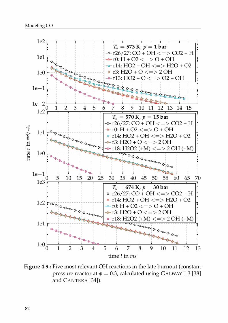
Modeling CO
0 1 2 3 4 5 6 7 8 9 10 11 12 13 14 151e−2
1e−1
1e0
1e1
1e2Tu = 573 K, p = 1 barr26/27: CO + OH <=> CO2 + Hr0: H + O2 <=> O + OHr14: HO2 + OH <=> H2O + O2r3: H2O + O <=> 2 OHr13: HO2 + O <=> O2 + OH
0 5 10 15 20 25 30 35 40 45 50 55 60 65 701e−1
1e0
1e1
1e2
rate
rin
mol/m
3 s
Tu = 570 K, p = 15 barr26/27: CO + OH <=> CO2 + Hr0: H + O2 <=> O + OHr14: HO2 + OH <=> H2O + O2r3: H2O + O <=> 2 OHr18: H2O2 (+M) <=> 2 OH (+M)
0 1 2 3 4 5 6 7 8 9 10 11 12 131e0
1e1
1e2
1e3
time t in ms
Tu = 674 K, p = 30 barr26/27: CO + OH <=> CO2 + Hr14: HO2 + OH <=> H2O + O2r0: H + O2 <=> O + OHr3: H2O + O <=> 2 OHr18: H2O2 (+M) <=> 2 OH (+M)
Figure 4.9.: Five most relevant OH reactions in the late burnout (constantpressure reactor at φ = 0.3, calculated using GALWAY 1.3 [38]and CANTERA [34]).
82

4.6 Application and Validation
In the following, it is assumed that all reactants on the left hand side ofthis set of equations are in equilibrium. The burnout of CO does not sig-nificantly alter O2 and water (H2O) as both species are available in abun-dance. Fast time scales can be assumed for the following radicals: Hydro-gen (H), oxygen (O), and hydroperoxyl (HO2). This leads to a model thatallows to tabulate the OH creation rate ςcr,OH prior to the CFD simulationand to evaluate the OH creation time scale by using:
τcr,OH =[OH]
ςcr,OH. (4.19)
τcr,OH is the built-up time for the equilibrium value of OH assuming thesimplified creation rate. Furthermore, a dimensionless identifier is em-ployed that describes the relationship between the time scales for OH cre-ation and CO oxidation:
ζOH =τcr,OH
τox,CO. (4.20)
A critical value of unity is used throughout the present work as this valueimplies the point at which CO oxidation exceeds OH creation.
4.6. Application and Validation
The CO modeling strategy is implemented in the software presented inAppendix A in addition to the combustion model. The model-specificflow of information is shown in Figure 4.10.
In the following, the application of the proposed CO model is shown. Inthe first Section 4.6.3, the model’s capability of dealing with specific sit-uations that are relevant for gas turbines at part load are demonstrated.For this purpose, a generic geometry featuring annularly distributed jetflames is employed. In addition, experiments in an atmospheric single-burner test rig have been carried out. The test rig has an unique com-bustion chamber design that allows the measurement of locally resolvedCO distributions. Validation of the atmospheric test rig is presented inSection 4.6.1. The last Section 4.6.2 shows the application of the modelto the GT11N’s silo combustor that comprises 37 burners. Two cases are
83

Modeling CO
f
κstψ
f , κ, ψ s∗c(κ, ψ, f
)
Γ(s∗c , s0c)
s0c(
f)
additional manifold
computationalgrid
adiabatic premixed
Ys( f , c)T( f , c)
ωc( f , c)PDF
integrated
Ys(c, c′′, f , f ′′)T(c, c′′, f , f ′′)
Y0CO(c, c′′, f , f ′′)
c, c′′, f , f ′′
viewer
unstretched,
tables
pre-
post-processing
counterflow flamelets
adiabatic premixedstretched, non-
counterflow flamelets
YOH,eq, YCO,eq
tables
ψ
Γψ,CO(ψ, f )
stretch evaluation(Sec. 3.2.1)
heat loss evaluation(Sec. 3.2.1)
stretch
(Sec. 3.2.3)evaluation
heat loss
(Sec. 3.2.2)evaluation
solving
κ
f
mκ,CO, mψ,CO
ψ
κ
processing
s0c( f ), ςcr,OH( f )
s∗c(κ0, ψ, f
)s∗c(κ, ψ0, f
)Γκ,CO(κ, f )
solverCFD
Y0OH(c, c′′, f , f ′′)
YCO,model(c, c′′, f , f ′′)
ςcr,OH( f )
YOH,eq( f )YCO,eq( f )
Figure 4.10.: Simplified overview of the CO model.
validated that differ in pressure and size. Moreover, both cases employdifferent concepts of fuel staging.
4.6.1. Atmospheric Single-Burner Test Rig
A novel combustion chamber design has been developed that allows thelocal measurement of CO. Note that locally resolved CO distributions are
84
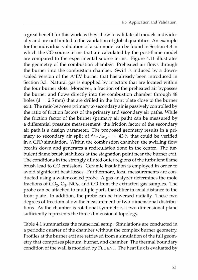
4.6 Application and Validation
a great benefit for this work as they allow to validate all models individu-ally and are not limited to the validation of global quantities. An examplefor the individual validation of a submodel can be found in Section 4.3 inwhich the CO source terms that are calculated by the post-flame modelare compared to the experimental source terms. Figure 4.11 illustratesthe geometry of the combustion chamber. Preheated air flows throughthe burner into the combustion chamber. Swirl is induced by a down-scaled version of the A2EV burner that has already been introduced inSection 3.3. Natural gas is supplied by injectors that are located withinthe four burner slots. Moreover, a fraction of the preheated air bypassesthe burner and flows directly into the combustion chamber through 48holes (d = 2.5 mm) that are drilled in the front plate close to the burnerexit. The ratio between primary to secondary air is passively controlled bythe ratio of friction factors of the primary and secondary air paths. Whilethe friction factor of the burner (primary air path) can be measured bya differential pressure measurement, the friction factor of the secondaryair path is a design parameter. The proposed geometry results in a pri-mary to secondary air split of m0,sec/m0,pri = 43 % that could be verifiedin a CFD simulation. Within the combustion chamber, the swirling flowbreaks down and generates a recirculation zone in the center. The tur-bulent flame brush stabilizes at the stagnation point near the burner exit.The conditions in the strongly diluted outer regions of the turbulent flamebrush lead to CO emissions. Ceramic insulation is employed in order toavoid significant heat losses. Furthermore, local measurements are con-ducted using a water-cooled probe. A gas analyzer determines the molefractions of CO2, O2, NOx, and CO from the extracted gas samples. Theprobe can be attached to multiple ports that differ in axial distance to thefront plate. In addition, the probe can be traversed radially. These twodegrees of freedom allow the measurement of two-dimensional distribu-tions. As the chamber is rotational symmetric, a two-dimensional planesufficiently represents the three-dimensional topology.
Table 4.1 summarizes the numerical setup. Simulations are conducted ina periodic quarter of the chamber without the complex burner geometry.Profiles at the burner exit are retrieved from a simulation of the full geom-etry that comprises plenum, burner, and chamber. The thermal boundarycondition of the wall is modeled by FLUENT. The heat flux is evaluated by
85

Modeling CO
insulation
gasinjection
air
probe
temperatureprobe λwall
lwall
850 mmd=
171
mm
dburner = 32 mm
d = 2.5 mm
3.5 mm
r = 26.5 mm
perforatedplate (48 holes)
Figure 4.11.: Illustration of the atmospheric single-burner test rig.
considering the thermal conductivity of the insulation (λwall = 0.15 W/mK)and the distance to the temperature measurement probes (lwall = 2.8 cm)that are attached as depicted in Figure 4.11. Figure 4.12 shows the velocityu in the upper half. The velocity distribution indicates that the secondaryair jets are able to penetrate the burner flow. The mixture fraction f isshown in the lower half of Figure 4.12. The significant dilution by sec-ondary air is evident. Numerically predicted CO distributions are shownin Figure 4.13. Moreover, the corresponding model zones are illustratedin Figure 4.14. Results for five different adiabatic flame temperatures Tad
are shown. Reactivity reduces for decreasing adiabatic flame tempera-ture and the turbulent flame brush ( ) moves downstream. CO emissionsclearly rise as the adiabatic flame temperature Tad decreases. The modeldescribes the rise in CO emissions by the following three mechanisms:
86
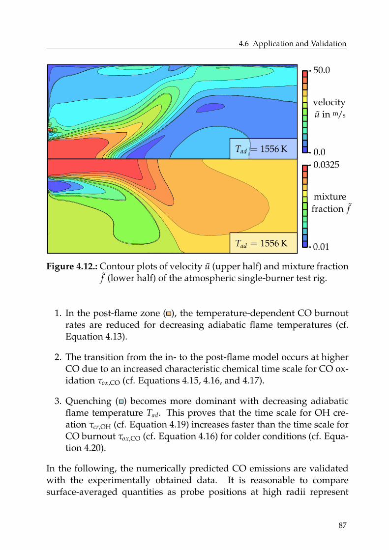
4.6 Application and Validation
50.0
0.0
0.01
0.0325
u in m/s
velocity
fraction fmixture
Tad = 1556 K
Tad = 1556 K
Figure 4.12.: Contour plots of velocity u (upper half) and mixture fractionf (lower half) of the atmospheric single-burner test rig.
1. In the post-flame zone ( ), the temperature-dependent CO burnoutrates are reduced for decreasing adiabatic flame temperatures (cf.Equation 4.13).
2. The transition from the in- to the post-flame model occurs at higherCO due to an increased characteristic chemical time scale for CO ox-idation τox,CO (cf. Equations 4.15, 4.16, and 4.17).
3. Quenching ( ) becomes more dominant with decreasing adiabaticflame temperature Tad. This proves that the time scale for OH cre-ation τcr,OH (cf. Equation 4.19) increases faster than the time scale forCO burnout τox,CO (cf. Equation 4.16) for colder conditions (cf. Equa-tion 4.20).
In the following, the numerically predicted CO emissions are validatedwith the experimentally obtained data. It is reasonable to comparesurface-averaged quantities as probe positions at high radii represent
87
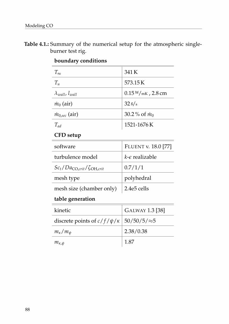
Modeling CO
Table 4.1.: Summary of the numerical setup for the atmospheric single-burner test rig.
boundary conditions
T∞ 341 K
Tu 573.15 K
λwall, lwall 0.15 W/mK , 2.8 cm
m0 (air) 32 g/s
m0,sec (air) 30.2 % of m0
Tad 1521-1676 K
CFD setup
software FLUENT v. 18.0 [77]
turbulence model k-ε realizable
Sct/DaCO,crit/ζOH,crit 0.7/1/1
mesh type polyhedral
mesh size (chamber only) 2.4e5 cells
table generation
kinetic GALWAY 1.3 [38]
discrete points of c/ f /ψ/κ 50/50/5/≈5
mκ/mψ 2.38/0.38
mκ,ψ 1.87
88
4.6 Application and Validation
larger surfaces than locations at low radii. Thus, each measured valueof CO is multiplied with the surface of its corresponding annulus. Fur-thermore, the products of all radii are summed up and divided by thetotal surface:
〈XCO,dry〉 =∑an Aan〈XCO,dry〉an
∑an Aan. (4.21)
Figure 4.15 shows the plot of measured CO mole fractions XCO ( ) as afunction of adiabatic flame temperature Tad for three different residencetimes. Residence times are estimated in a corresponding CFD simulation.For this purpose, Lagrangian observers are simulated in order to createstreamlines. Moreover, the corresponding residence times of fluid particle(represented by the Lagrangian observers) can be analyzed as a functionof the location.
Using the CO model proposed in this chapter ( ) leads to good agree-ment with the experimental data. The model performance apparently de-creases for cold conditions. Note that the proposed model assumes thatall intermediate species are in equilibrium and solely CO decreases dur-ing burnout. This assumption may be invalid for adiabatic temperaturesthat are below a critical limit. An example to this mechanism is givenby the frequently observed occurrence of unburnt hydrocarbon emissionsnear the lean blowout limit. This model deficiency is not a major draw-back as the numerical prediction of CO emissions is solely relevant foroperating points that show emissions that are in the technically relevantrange. Note that emission legislations are usually below 100 ppmv. Inaddition, Figure 4.15 shows the predictions by an adiabatic version of theCO model ( ) in order to characterize the influence of heat loss on CO.Even though the ceramic insulation is able to avoid major heat losses, asignificant decrease of CO is evident when non-adiabatic effects are notconsidered.
As it is discussed above, flamelet-based combustion models are not ableto predict CO. This is argued by the assumption of infinitely thin reactionzones that cannot be used to describe the burnout of CO. Consequently,the combustion model ( ) wrongly predicts fully burnt out CO as theturbulent flame brush is located upstream of the measurement locations.
89

Modeling CO
0.0
199
224.5
250
Tad = 1521 K
0 8e3XCO in ppmv
CO mole fraction
Tad = 1556 K
Tad = 1604 K
Tad = 1646 K
Tad = 1676 K
Figure 4.13.: Contour plots of CO mole fraction XCO of the atmosphericsingle-burner test rig.
90
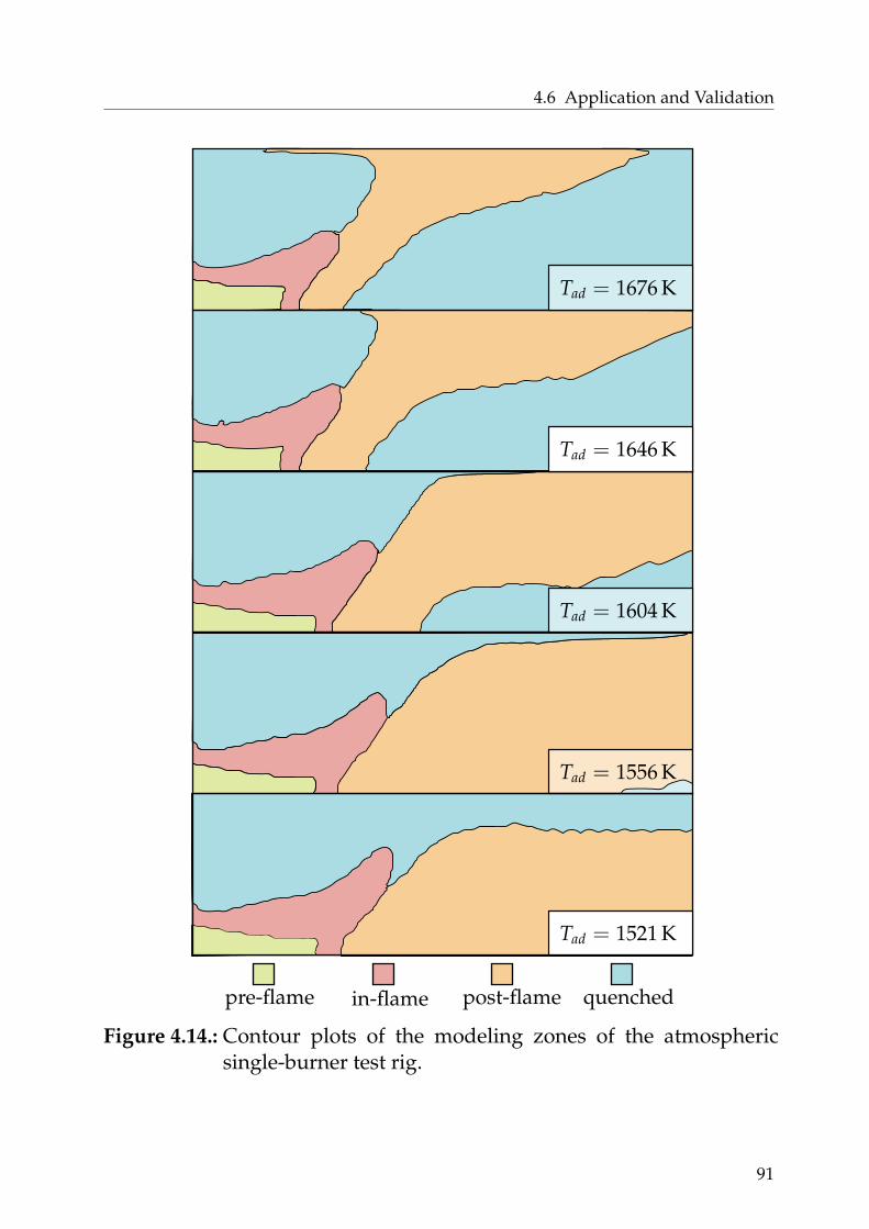
4.6 Application and Validation
pre-flame in-flame post-flame quenched
Tad = 1646 K
Tad = 1604 K
Tad = 1521 K
Tad = 1676 K
Tad = 1556 K
Figure 4.14.: Contour plots of the modeling zones of the atmosphericsingle-burner test rig.
91

Modeling CO
0
500
1000
1500
2000x = 199 cm, τ ≈ 18 msCO measurementsCO modelCO model (adiabatic)combustion model
0
500
1000
1500
2000
CO
mol
efr
acti
on〈X
CO〉i
npp
mv
x = 224.5 cm, τ ≈ 22 ms
1520 1540 1560 1580 1600 1620 16400
500
1000
adiabatic temperature Tad in K
x = 250 cm, τ ≈ 26 ms
Figure 4.15.: Temperature dependent CO emissions of the atmosphericsingle-burner test rig, which is illustrated in Figure 4.11.
92

4.6 Application and Validation
4.6.2. Multi-Burner Cases
Two multi-burner cases that employ fuel staging concepts are presentedin the following. Both cases use the GT11N silo combustor geometry thatcomprises 37 burners, which is illustrated in Figure 4.16. In addition, thefuel staging concept of the atmospheric model is depicted. The first vali-dation case is a down-scaled, atmospheric model of the GT11N. In addi-tion, validation of a full-scale GT11N in field operation is presented. Anoverview of the numerical setups is given in Table 4.2. Both cases oper-ate under part-load conditions in which solely a part of the total amountof burners is active. Multiple stages exist that differ in their number ofactive burners. A specified group of burners is switched off during thetransition to a colder stage. By reducing the power to part load, severalstages are passed and the number of burners is successively reduced. Thedecisive difference between both cases is the way fuel is reduced before agroup of burners is switched off:
• Atmospheric GT11N model: A group of burners is ramped downfrom reference conditions to pure air. Variation of load during a stageis conducted by solely changing the fuel supply of the specific groupthat is intended to get switched off.
• High-pressure GT11N in field operation: The reduction of load isaccomplished by decreasing the fuel supply for all active burners.This can be done until CO emissions increase to a specific limit.When this limit is reached, a group of burners that operates at sta-ble conditions is abruptly switched off. The fuel surplus from theswitched off burners is redistributed to the remaining group of ac-tive burners leading to a drop in CO emissions.
4.6.2.1. Atmospheric Model of the GT11N
The validation of a down-scaled, atmospheric model of the GT11N is pre-sented in the following. The experimental data are retrieved from an un-published, company-internal measurement study that was conducted inorder to find reasonable fuel staging strategies for silo combustors. Inthe report, the optimal concept for part-load operation is investigated
93
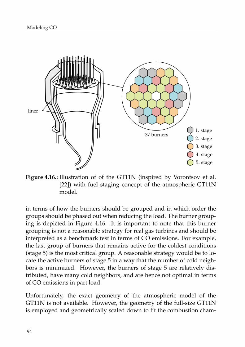
Modeling CO
200, Grays, not smooth
wall
non-adiabatic
periodic
boundary
staged
unstaged
60 ◦
wall
adiabatic
piece
transition
37 burner
liner
pilot group
active burners
ignition
37 burners
liner
2. stage
3. stage
4. stage
5. stage
1. stage
37 burners
liner
2. stage
3. stage
4. stage
5. stage
1. stage
prev: height 78
Figure 4.16.: Illustration of of the GT11N (inspired by Vorontsov et al.[22]) with fuel staging concept of the atmospheric GT11Nmodel.
in terms of how the burners should be grouped and in which order thegroups should be phased out when reducing the load. The burner group-ing is depicted in Figure 4.16. It is important to note that this burnergrouping is not a reasonable strategy for real gas turbines and should beinterpreted as a benchmark test in terms of CO emissions. For example,the last group of burners that remains active for the coldest conditions(stage 5) is the most critical group. A reasonable strategy would be to lo-cate the active burners of stage 5 in a way that the number of cold neigh-bors is minimized. However, the burners of stage 5 are relatively dis-tributed, have many cold neighbors, and are hence not optimal in termsof CO emissions in part load.
Unfortunately, the exact geometry of the atmospheric model of theGT11N is not available. However, the geometry of the full-size GT11Nis employed and geometrically scaled down to fit the combustion cham-
94

4.6 Application and Validation
ber’s diameter of the atmospheric model. The geometry comprises theplenum, all burners, the combustion chamber, and the transition piece.
CO mole fraction XCO as a function of adiabatic flame temperature Tad isplotted in Figure 4.17. Four stages are indicated. In each stage, a speci-fied group of burners is ramped down from reference conditions to pureair. The hot conditions of the first stage lead to fast CO burnout. Hence,measured CO ( ) as well as modeled CO ( ) are close to equilibrium.In the second stage, CO emissions rise by reducing the fuel supply of thespecified group of burners ( ) from 100 % to 50 %. This mechanism isshown by the first two contour plots of Figure 4.18. Moreover, reducingthe fuel supply from 50 % to 0 % leads to a decrease of CO emissions.Here, the specified group of burners operates below lean blowout limitand are piloted by the active group ( ). This mechanism is shown inthe third contour plot of Figure 4.18. The decline in CO with decreasingfuel supply is based on the mechanism that the amount of carbon atomsdecreases with fuel supply. The third stage also shows an increase of COemissions when the burners are reduced in fuel supply. A decisive differ-ence between the second and the third stage is that the global CO emis-sions do not decline after the specified group of burners is phased out. Atthis point, the burnout of the active burners cannot be achieved anymore.In the fourth stage, the typical rise and fall of CO emissions during theprocess of phasing out a group of burners is shown. The proposed COmodel strategy is capable of meeting the global CO measurements of thesecond and third stage. In the fourth stage, experimental CO declines af-ter a local maximum was reached. The experimental profile of the fourthstage cannot be predicted by the proposed modeling strategy as CO pro-ceeds rising instead of dropping as it is observed in the experiments. COpredicted by the combustion model ( ) is again tremendously underes-timating global CO.
95
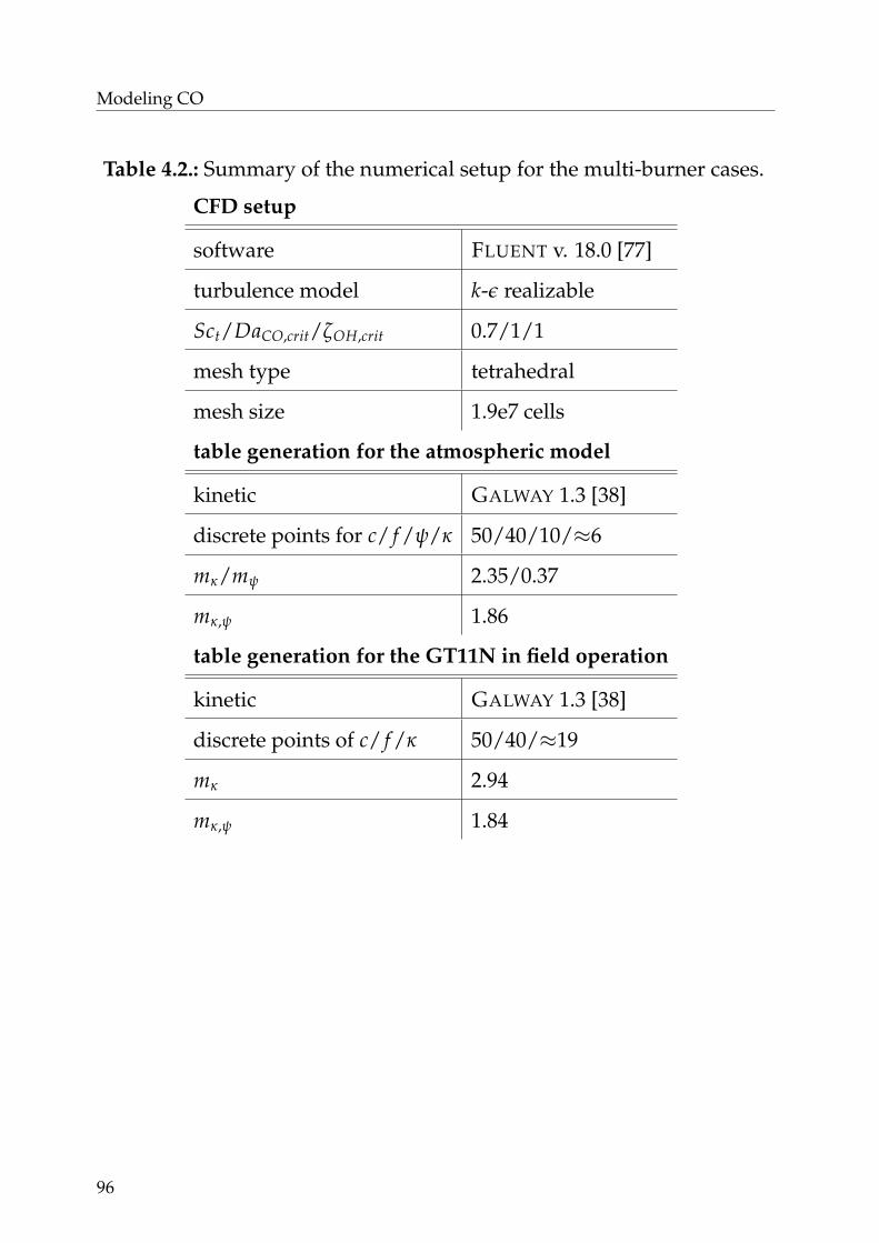
Modeling CO
Table 4.2.: Summary of the numerical setup for the multi-burner cases.
CFD setup
software FLUENT v. 18.0 [77]
turbulence model k-ε realizable
Sct/DaCO,crit/ζOH,crit 0.7/1/1
mesh type tetrahedral
mesh size 1.9e7 cells
table generation for the atmospheric model
kinetic GALWAY 1.3 [38]
discrete points for c/ f /ψ/κ 50/40/10/≈6
mκ/mψ 2.35/0.37
mκ,ψ 1.86
table generation for the GT11N in field operation
kinetic GALWAY 1.3 [38]
discrete points of c/ f /κ 50/40/≈19
mκ 2.94
mκ,ψ 1.84
96

4.6 Application and Validation
0.4 0.5 0.6 0.7 0.8 0.9 10
0.2
0.4
0.6
0.8
1
1.2
1.4
1.6
fourthstage
thirdstage
secondstage
firststage
#1#2
#3
normalized adiabatic flame temperature Tad
norm
aliz
edC
Om
ole
frac
tion
XC
O,d
ry
CO measurementsCO modelcombustion model
Figure 4.17.: Temperature dependent CO emissions of the atmosphericGT11N model.
97
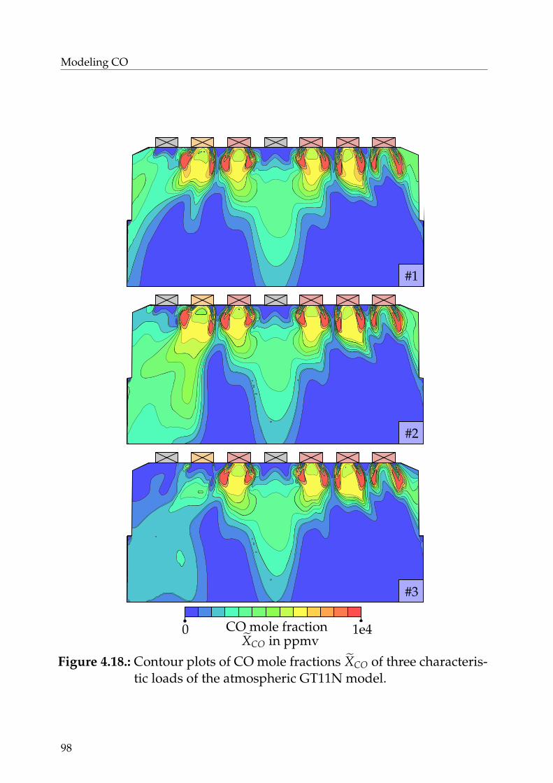
Modeling CO
piloted groupstaged groupignition burner
0 1e4CO mole fractionXCO in ppmv
#3
19
20
18
17
#2
#1
Figure 4.18.: Contour plots of CO mole fractions XCO of three characteris-tic loads of the atmospheric GT11N model.
98

4.6 Application and Validation
4.6.2.2. High-Pressure GT11N in Field Operation
The burner layout that is used in the high-pressure case is illustratedin Figure 4.19. 31 single switchable burners are belonging to the maingroup ( ). The central burner is not active for the operating points thatare considered in this study. Burners of the piloted group ( ) are locatedin each corner. Piloted burners are supplied with substantially less fuelthan burners that belong to the main group. Figure 4.21 demonstratesthe interaction between the two groups. The first contour plot shows thelaminar flame velocity sl. It can be seen that burners of the piloted group( ) are operated with laminar flame velocities that are close to zero andare thus not able to provide a stable flame. Nevertheless, burnout canbe achieved as adjacent active burners from the main group ( ) are ableto burnout the cold flow of the piloted group. The second contour plotof Figure 4.21 shows the interaction of active burners with an inactiveburner ( ) that is located in the center. It is apparent that the cold cen-tral burner has a strong impact on the CO emissions. The third contourplot shows the result when the quenching model is deactivated in orderto demonstrate its significant impact on CO oxidation.
Validation is performed by comparing modeled with measured CO emis-sions as function of adiabatic flame temperature Tad in Figure 4.20. Nu-merical results ( ) are in good agreement with the measured data ( ).The proposed modeling strategy is apparently able to quantitatively pre-dict the absolute CO emissions, as well as the influence of burner switch-off events on CO. A decreased model accuracy can be observed in verylean conditions that was already discussed above. Additionally, predic-tions from the flamelet-based combustion model are plotted ( ). As ex-pected, the flamelets do not reach the combustor’s outlet and CO is dras-tically underestimated.
99
Modeling CO
piloted group
main group
Figure 4.19.: Burner layout of the high-pressure GT11N in field operation.
0.7 0.75 0.8 0.850
0.2
0.4
0.6
0.8
1
three burnerswitch-off events
normalized adiabatic flame temperature Tad
norm
aliz
edC
Om
ole
frac
tion
XC
O,d
ry
CO measurementsCO modelcombustion model
Figure 4.20.: Temperature dependent CO emissions of the high-pressureGT11N in field operation.
100
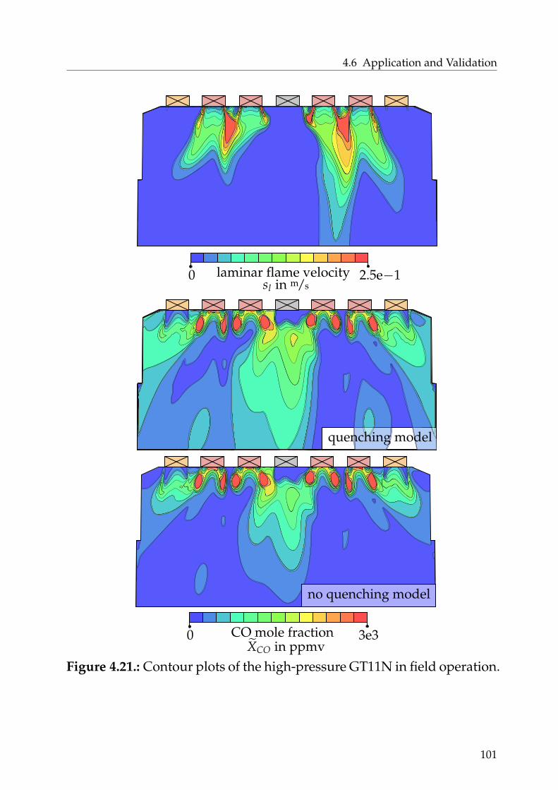
4.6 Application and Validation
0 2.5e−1laminar flame velocitysl in m/s
piloted groupstaged groupignition burner
0 3e3CO mole fractionXCO in ppmv
no quenching model
quenching model
Figure 4.21.: Contour plots of the high-pressure GT11N in field operation.
101

Modeling CO
secondary groupprimary group
non-adiabaticwall
periodic boundarycondition
60 ◦
160 mm
160 mm
r = 40 mm
d = 12 mm65
mm
Figure 4.22.: Illustration of the novel combustor concept that is inspiredby Lammel et al. [90]).
4.6.3. Application to a Novel Combustor Concept
Figure 4.22 illustrates the in this section used geometry that is inspiredby Lammel et al. [89]. Annularly distributed inlets supply jet flames thatare close enough to each other to feature intense flame interaction. Allnozzles have a diameter of 12 mm and are located at an distance to thecombustor center of 40 mm. The combustor’s diameter is 130 mm and hasa length of 160 mm. Note that the boundary conditions are retrieved fromLammel et al. [90]. The combustor is operated at a reference pressure ofp = 8 bar. Moreover, fuel is a mixture of CH4 (XCH4,1 = 0.6) and dihydro-gen (H2) (XH2,1 = 0.40). Heat loss is imposed by considering an infinitelythin wall, an outer heat loss coefficient of α = 50 W/m2K and an ambienttemperature of T∞ = 300 K. Further details of the boundary conditionsand the numerical setup are summarized in Table 4.3.
102
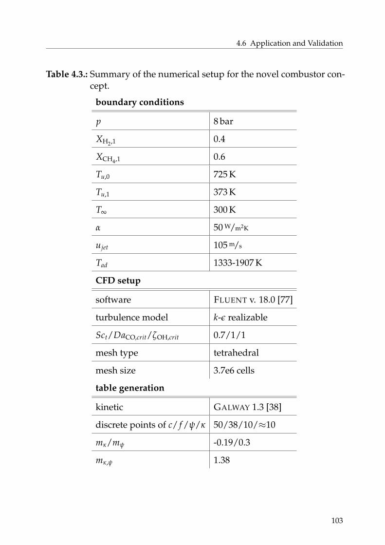
4.6 Application and Validation
Table 4.3.: Summary of the numerical setup for the novel combustor con-cept.
boundary conditions
p 8 bar
XH2,1 0.4
XCH4,1 0.6
Tu,0 725 K
Tu,1 373 K
T∞ 300 K
α 50 W/m2K
ujet 105 m/s
Tad 1333-1907 K
CFD setup
software FLUENT v. 18.0 [77]
turbulence model k-ε realizable
Sct/DaCO,crit/ζOH,crit 0.7/1/1
mesh type tetrahedral
mesh size 3.7e6 cells
table generation
kinetic GALWAY 1.3 [38]
discrete points of c/ f /ψ/κ 50/38/10/≈10
mκ/mψ -0.19/0.3
mκ,ψ 1.38
103

Modeling CO
4.6.3.1. The Influence of Swirl on CO Emissions
The influence of swirl on CO emissions is investigated by comparing jetflames with swirl flames. Swirl is imposed by using profiles of the A2EVburner that are scaled down to the nozzle’s diameter. It is worth not-ing that the axial velocity component of the swirled flow equals the jetsin order to realize the same mass flows in both configurations. In Fig-ure 4.23, the resulting distributions of CO mole fraction XCO is shown forboth configurations. The flow topology substantially changes when swirlis imposed. While the jet flames show a heat release zone that is locatedin the center of the combustor, the turbulent flame brush of the swirledcase stabilizes close to the burner exit. It is evident that the swirled caseis beneficial in terms of burnout as the residence time behind the flame ishigher in comparison to the jet flames. In order to investigate CO emis-sions as a function of adiabatic flame temperature Tad, fuel mass flow isdecreased evenly for all burners. The corresponding results are plotted inFigure 4.24. A sharp increase in CO emissions occurs for both cases afterthe adiabatic temperature has fallen below a critical level. In both config-urations, the residence time behind the flame is not long enough to fullyburnout CO. The jet flame configuration ( ) shows elevated CO whenthe adiabatic flame temperature Tad drops below 1677 K. The swirl flames( ) show global CO that is in equilibrium for adiabatic flame tempera-ture above 1620 K. Remarkably, CO emissions rise for both cases with asimilar slope, although the flow topology differs significantly.
4.6.3.2. The Influence of Colder Neighbors on CO Emissions
As shown in the previous section, the unstaged jet configurations cannotbe operated below a critical flame temperature of about 1600 K. In thefollowing, the advantages of fuel staging are demonstrated by using thejet configuration. As mentioned before, lower global adiabatic flame tem-peratures can be realized by applying fuel staging concepts when a stableflame act as a premixed pilot in order to burn out flames that a reducedin fuel supply. This case aims to study the situation in multi-burner sys-tems in which active burners interact with adjacent, colder burners. Twogroups of burners are specified as shown in Figure 4.22. The secondary
104

4.6 Application and Validation
0 6.5e3CO mole fraction
fre f
Tad = 1735 Kfre f
XCO in ppmv
jets
swirl flames
Figure 4.23.: Comparison of jet with swirl flames at an adiabatic temper-ature of Tad = 1620 K of the novel combustor concept.
1400 1500 1600 1700 1800 19000
50
100
150
200
250
300
Tad in K
XC
O,1
5,dr
yin
ppm
v
unstaged burners (jets)unstaged burners (swirled)fuel-staged case (jets)equilibrium
Figure 4.24.: Temperature dependent CO emissions of the novel combus-tor concept.
105
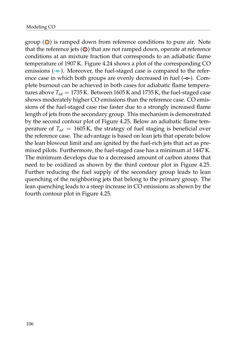
Modeling CO
group ( ) is ramped down from reference conditions to pure air. Notethat the reference jets ( ) that are not ramped down, operate at referenceconditions at an mixture fraction that corresponds to an adiabatic flametemperature of 1907 K. Figure 4.24 shows a plot of the corresponding COemissions ( ). Moreover, the fuel-staged case is compared to the refer-ence case in which both groups are evenly decreased in fuel ( ). Com-plete burnout can be achieved in both cases for adiabatic flame tempera-tures above Tad = 1735 K. Between 1605 K and 1735 K, the fuel-staged caseshows moderately higher CO emissions than the reference case. CO emis-sions of the fuel-staged case rise faster due to a strongly increased flamelength of jets from the secondary group. This mechanism is demonstratedby the second contour plot of Figure 4.25. Below an adiabatic flame tem-perature of Tad = 1605 K, the strategy of fuel staging is beneficial overthe reference case. The advantage is based on lean jets that operate belowthe lean blowout limit and are ignited by the fuel-rich jets that act as pre-mixed pilots. Furthermore, the fuel-staged case has a minimum at 1447 K.The minimum develops due to a decreased amount of carbon atoms thatneed to be oxidized as shown by the third contour plot in Figure 4.25.Further reducing the fuel supply of the secondary group leads to leanquenching of the neighboring jets that belong to the primary group. Thelean quenching leads to a steep increase in CO emissions as shown by thefourth contour plot in Figure 4.25.
106
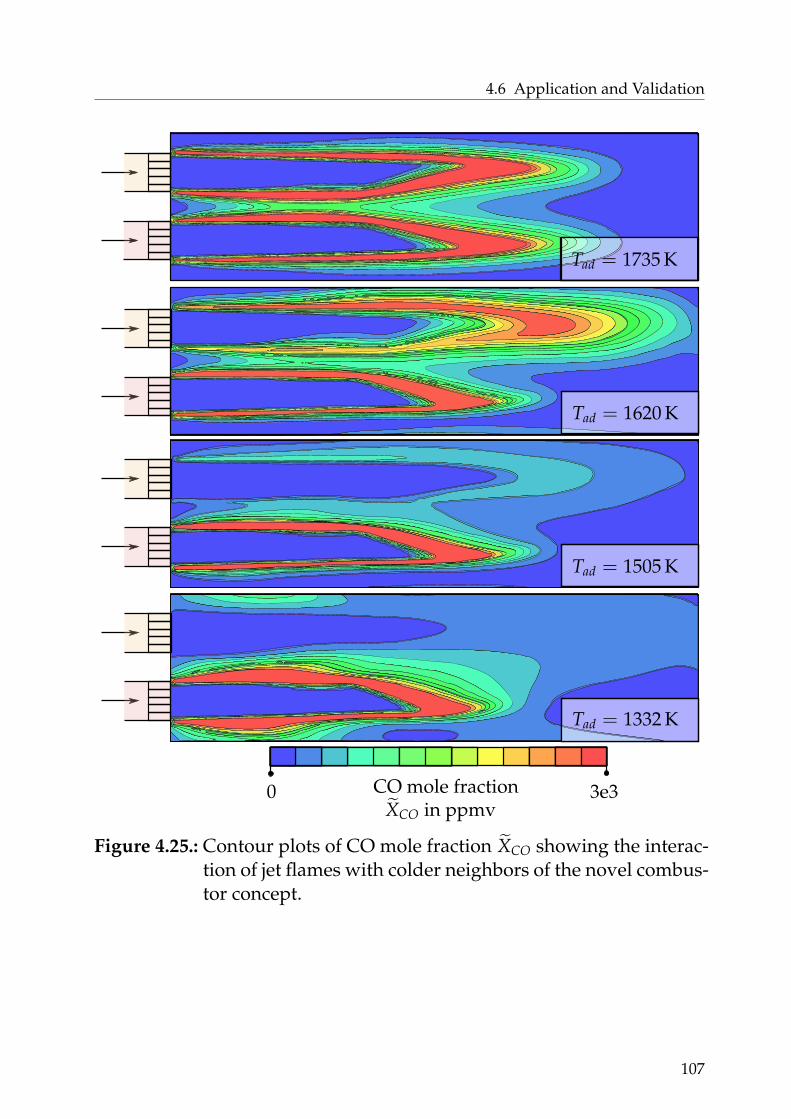
4.6 Application and Validation
Tad = 1620 K
Tad = 1505 K
Tad = 1332 K
0.5 f 0
f 0
f 0
f 0
0.3 f 0
0. f 0
0 3e3CO mole fractionXCO in ppmv
Tad = 1735 K
Figure 4.25.: Contour plots of CO mole fraction XCO showing the interac-tion of jet flames with colder neighbors of the novel combus-tor concept.
107

5 Summary
This study investigates combustion and CO emissions in cold conditionsthat occur in gas turbines that operate at part load conditions. Althoughthe prediction of CO emissions is a fundamental problem with manypractical applications, no satisfying model has been published so far. Asshown in this work, the inability of existing models to predict CO is basedon two reasons:
• Combustion models often lack accuracy in cold conditions.
• In order to successfully predict CO emissions, a wide range of under-lying time scales need to be considered.
The solution that is proposed in this work, solves both problems individ-ually and hence comprises the following two parts:
Combustion modeling in turbulent, partially-premixed conditions is cov-ered in the first part. The FGM theory is adopted in this work by employ-ing manifolds that are generated by freely-propagating flamelets. Thecombustion process at cold conditions is demonstrated to be particularlysusceptible for flame stretch and heat loss. An approach to efficientlyconsider both effects in the context of FGM is presented. For this pur-pose, an additional manifold is introduced that tabulates premixed coun-terflow flamelets at various enthalpy levels. The novel combustion mod-eling strategy is validated using experimental data from an atmosphericsingle-burner test rig. Key findings can be summarized by the following:
• Significant improvement in terms of flame shape and position isachieved by considering flame stretch and heat loss.
109
Summary
• The performance of the presented methodology is compared to thenumerical predictions by EDM and TFC. Both standard combustionmodels and the original FGM formulation significantly overestimatechemical rates in regions that feature high flame stretch rates and/orheat loss.
The second part of this study investigates the formation and oxidationof CO. CO chemistry occurs in a wide spectrum of time scales leadingto major challenges for the modeling approach. While the radical-drivenchemistry within the turbulent flame brush occurs at short time scales, theburnout behind the heat release zone is based on significantly longer timescales. A novel strategy is presented that divides the domain in multiplezones by identifying the critical time scale that dominates CO chemistry.For each zone, a new model is developed to close CO:
• In-flame zone: A model is introduced that employs CO profiles fromone-dimensional flamelet calculations and considers the influence ofheat loss and flame stretch.
• Post-flame zone: Reduced chemistry is employed to close CO forkinetically-limited conditions.
• Quenching zone: The reasons for quenching are identified and mod-eled on the basis of chemical time scales.
The developed methodology is applied to various cases which lead to thefollowing key findings:
• Atmospheric single-burner test rig: A test rig is introduced that wasbuilt to carry out experiments of a single swirl flame, which stronglyinteracts with secondary air. The test rig facilitates the measurementof locally resolved CO distributions, which allows to validate the in-and post-flame zone individually. The results of the validation canbe summarized as follows:
– The predicted CO is in good agreement with the experiments.
– A decrease of the model’s accuracy is observed for conditionsthat are close to the lean blowout limit.
110
– CO predicted by the flamelet-based combustion model is shownto tremendously underestimate the experimental data.
• Multi-burner systems with fuel staging concepts: The modelingstrategy is applied to two different multi-burner cases. In the firstcase, a down-scaled, atmospheric model of the GT11N silo com-bustor is employed. Moreover, the second case is a high-pressure,full-scale GT11N in field operation. Both cases employ fuel-stagingstrategies but differ in the way fuel is reduced before a group of burn-ers is switched off. The main findings are summarized as follows:
– The combustion model is not able to predict CO emissions.
– The CO model’s ability to meet global emissions is shown.
– Characteristics from the fuel staging concepts are well captured.
• Novel Combustor Concept: The application of the proposed mod-eling strategy to a novel combustor concept is demonstrated. Thetest rig comprises twelve annularly distributed nozzles that supplystrongly interacting flames. The model’s capability to capture thefollowing phenomena is shown:
– The influence of swirl on CO emissions is investigated by com-paring jet with swirl flames.
– Advantages of fuel staging are discussed by comparing an un-staged with a staged case.
This work shows the first modeling strategy that is able to successfullypredict CO emissions in a way that it can be practically used for the de-velopment of new combustors in the industry. Moreover, the followingtwo key messages can be concluded from this work:
• Neglecting flame stretch and heat loss in cold conditions may signif-icantly decrease the combustion model’s accuracy.
• Modeling CO requires to develop models that are beyond the as-sumption of infinitely thin reactions zones.
111


A Software Implementation
A software package is written in order to provide a convenient solutionfor users to apply the models that are introduced in Chapter 3 and 4.In the following, details to the implementation are provided. Note thatthe model-specific flow of information was shown in the Figures 3.6 and4.10. Figure A.1 provides a simplified overview of the two elements thesoftware implementation consists of:
1. Table Generator: The proposed models are based on flamelet calcu-lations that are performed by the Table Generator prior to the CFDsimulation. Moreover, the solution of the flamelet simulations isstored in tables. An introduction to the Table Generator is providedin Section A.
2. User Defined Function: C-based User Defined Functions can be em-ployed to extend the functionality of the commercial CFD softwareFLUENT [77]. During runtime, the solver executes the code in orderto calculate the proposed modeling strategy. Details to the imple-mentation of the User Defined Functions are provided in Section A.
software
tables
FLUENT v.18User Defined
Table Generator
Functions
Sec. A
Sec. Aimplementation
Figure A.1.: Overview of the software implementation.
113
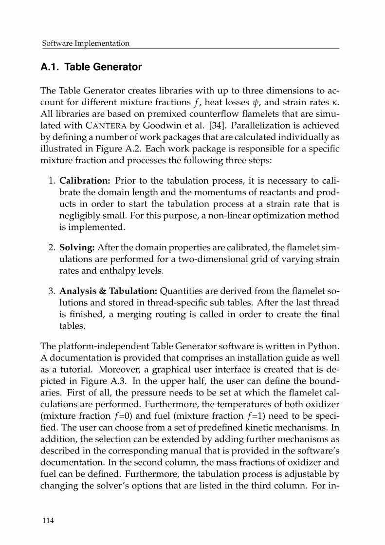
Software Implementation
A.1. Table Generator
The Table Generator creates libraries with up to three dimensions to ac-count for different mixture fractions f , heat losses ψ, and strain rates κ.All libraries are based on premixed counterflow flamelets that are simu-lated with CANTERA by Goodwin et al. [34]. Parallelization is achievedby defining a number of work packages that are calculated individually asillustrated in Figure A.2. Each work package is responsible for a specificmixture fraction and processes the following three steps:
1. Calibration: Prior to the tabulation process, it is necessary to cali-brate the domain length and the momentums of reactants and prod-ucts in order to start the tabulation process at a strain rate that isnegligibly small. For this purpose, a non-linear optimization methodis implemented.
2. Solving: After the domain properties are calibrated, the flamelet sim-ulations are performed for a two-dimensional grid of varying strainrates and enthalpy levels.
3. Analysis & Tabulation: Quantities are derived from the flamelet so-lutions and stored in thread-specific sub tables. After the last threadis finished, a merging routing is called in order to create the finaltables.
The platform-independent Table Generator software is written in Python.A documentation is provided that comprises an installation guide as wellas a tutorial. Moreover, a graphical user interface is created that is de-picted in Figure A.3. In the upper half, the user can define the bound-aries. First of all, the pressure needs to be set at which the flamelet cal-culations are performed. Furthermore, the temperatures of both oxidizer(mixture fraction f =0) and fuel (mixture fraction f =1) need to be speci-fied. The user can choose from a set of predefined kinetic mechanisms. Inaddition, the selection can be extended by adding further mechanisms asdescribed in the corresponding manual that is provided in the software’sdocumentation. In the second column, the mass fractions of oxidizer andfuel can be defined. Furthermore, the tabulation process is adjustable bychanging the solver’s options that are listed in the third column. For in-
114
A.1 Table Generator
calibration
Table Generator
preprocessing solving
Sec. A
mixture fraction f [0]
routine
analysis &tabulation
solving flamelets for allstrain rates κheat losses ψ
thread 2:
thread 1:
mixture fraction f [1]
thread n:mixture fraction f [n-1]
sub tables 1
mergingroutine
final tables
sub tables n
sub tables 2
Figure A.2.: The work is divided in multiple threads that can be calcu-lated in parallel.
stance, the number of points that are used to discretize the mixture frac-tion and the enthalpy defect can be changed. Moreover, a characteristicmixture fraction needs to be specified that defines the mixture fraction atwhich the exponential factors m (cf. Equation 3.7, 4.5, and 4.7) should beevaluated. Note that it is best practice to specify a characteristic mixturefraction that corresponds to the expected average mixture fraction of theturbulent flame brush. In addition, the maximum values for strain andenthalpy can be changed by setting the corresponding entries. The refine-
115

Software Implementation
Figure A.3.: Graphical user interface of the Table Generator.
116
A.2 User Defined Function
ment level of the flamelet simulation is adjustable by selecting one of thethree predefined levels. In order to significantly speed up the calculation,a number of threads should be allocated in order to distribute the workpackages. In the lower half of the graphical user interface that is depictedin Figure A.3, different information is provided during run time in orderto inform the user of the actual progress. Besides the elapsed time and aprogress bar, one can find detailed information for each thread.
A.2. User Defined Function
The C-based User Defined Function can be interpreted as a model layerthat is located between the tables and the FLUENT [77] solver. The FLU-ENT extension consists of three modules that can be described as follows:
1. Reading module: This module is called before the solving processstarts. It loads the data that is stored in tables into memory. This isnecessary in terms of efficiency, as costly file operations during runtime are avoided.
2. Model module: All models that are proposed in this work are eval-uated by executing this module. It is hence necessary to call this partin every cell and for every iteration/time step. The module manip-ulates the source terms of the reaction progress variable and closesthe transport equation for CO according to the proposed modelingstrategy.
3. Interpolation module: In this module, the discrete in-memory datais interpolated. The interpolation routines are called several times forevery cell and for every iteration as a number of interpolated quan-tities are required to calculate the models. Even though the interpo-lation routine has the highest computational effort, the overhead isusually negligible.
117


B Additional Reaction Analysis
The CO model that was proposed in Chapter 4 is based on the analysis ofreactions in the late burnout of CO at an equivalence ratio of φ = 0.3. InFigure 4.4, the most relevant reactions for CO are plotted in order to showthat the post-flame model can be reduced to Equation r26/27. Moreover,Figure 4.9 shows the five most relevant reaction equations that describeOH to argue that solely r0, r3, and r14 can be used to describe the OHcreation source term.
In the following, both studies are repeated for an equivalence ratio ofφ = 0.5 in Figure B.1 and B.2.
119

Additional Reaction Analysis
0 0.1 0.2 0.3 0.4 0.5 0.6 0.7 0.8 0.91e−4
1e−2
1e0
1e2
1e4 Tu = 573 K, p = 1 barr26/27: CO + OH <=> CO2 + Hr24: CO + O (+M) <=> CO2 (+M)r30: HCO + O2 <=> CO + HO2r28: CO + HO2 <=> CO2 + OH
0 5 · 10−2 0.1 0.15 0.2 0.25 0.3 0.351e−31e−21e−1
1e01e11e21e3 Tu = 570 K, p = 15 bar
0 2 · 10−24 · 10−26 · 10−28 · 10−2 0.1 0.12 0.14 0.16
1e−2
1e−1
1e0
1e1
1e2
1e3
1e4 Tu = 674 K, p = 30 bar
Figure B.1.: Four most relevant CO reactions in the late burnout (constantpressure reactor at φ = 0.5, calculated using GALWAY 1.3 [38]and CANTERA [34]).
120
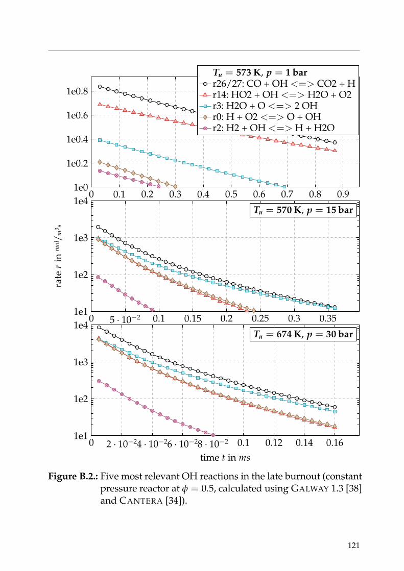
0 0.1 0.2 0.3 0.4 0.5 0.6 0.7 0.8 0.91e0
1e0.2
1e0.4
1e0.6
1e0.8
Tu = 573 K, p = 1 barr26/27: CO + OH <=> CO2 + Hr14: HO2 + OH <=> H2O + O2r3: H2O + O <=> 2 OHr0: H + O2 <=> O + OHr2: H2 + OH <=> H + H2O
0 5 · 10−2 0.1 0.15 0.2 0.25 0.3 0.351e1
1e2
1e3
1e4
rate
rin
mol/m
3 s
Tu = 570 K, p = 15 bar
0 2 · 10−24 · 10−26 · 10−28 · 10−2 0.1 0.12 0.14 0.161e1
1e2
1e3
1e4
time t in ms
Tu = 674 K, p = 30 bar
Figure B.2.: Five most relevant OH reactions in the late burnout (constantpressure reactor at φ = 0.5, calculated using GALWAY 1.3 [38]and CANTERA [34]).
121

Bibliography
Bibliography
[1] Intergovernmental Panel on Climate Change (IPCC), 2013.“Klimaanderung 2013 - Naturwissenschaftliche Grundlagen”.pp. 1–28.
[2] International Energy Agency (IEA), 2014. “World Energy Outlook2014 - Factsheet”. pp. 1–5.
[3] International Energy Agency (IEA), 2017. “World Energy Outlook2017 - Executive Summary”. pp. 1–13.
[4] British Petroleum (BP), 2018. “Energy Outlook”. pp. 1–125.
[5] United Nations (UN), 2015. “Paris Agreement under the United Na-tions Framework Conventions on Climate Change”. In 21st Confer-ence of the Parties, pp. 1–25.
[6] United Nations (UN), 1998. “Kyoto Protocol to the United NationsFramework Conventions on Climate Change”. In International Cli-mate Summit in Kyoto, pp. 1–20.
[7] Wiedermann, A., 2010. “Gasturbinentypen - eine Ubersicht”. InStationare Gasturbinen, 2nd ed. Springer-Verlag Berlin Heidelberg,Berlin, ch. 1, pp. 1–11.
[8] Union for the Coordination of Transmission of Electricity (UCTE),2004. “Operation Handbook - Appendix 1 - Load-Frequency Controland Performance”. pp. 1–27.
[9] Sinn, H. W., 2017. “Buffering Volatility: A Study on the Limits of Ger-many’s Energy Revolution”. European Economic Review, 99, pp. 130–150.
123
Bibliography
[10] BMWi - Bundesministerium fur Wirtschaft und Energie, 2016. “DieEnergie der Zukunft - Funfter Monitoring-Bericht zur Energiewende- Berichtsjahr 2015”. pp. 1–154.
[11] FNB-Gas - Die Fernleitungsbetreiber, 2016. “NetzentwicklungsplanGas 2018-2028”. pp. 1–204.
[12] Bundesnetzagentur, 2017. “Monitoringbericht 2017”. pp. 1–489.
[13] Sattelmayer, T., 2010. “Grundlagen der Verbrennung in stationarenGasturbinen”. In Stationare Gasturbinen, 2nd ed. Springer-VerlagBerlin Heidelberg, Berlin, ch. 9, pp. 397–453.
[14] Moning, R., and Waltke, U., 2010. “Verdichter”. In Stationare Gas-turbinen, 2nd ed. Springer-Verlag Berlin Heidelberg, Berlin, ch. 7,pp. 313–369.
[15] Lefebvre, A. H., and Ballal, D. R., 2010. Gas Turbine Combustion -Alternative Fuels and Emissions, 3rd ed. Taylor & Francis Group, BocaRaton.
[16] Steinbach, C., Ulibarri, N., Garay, M., Lubcke, H., Meeuwissen, T.,Haffner, K., Aubry, J., and Kodim, D., 2006. “Combustion Opti-mization for the Alstom GT13E2 Gas Turbine”. In Proceedings ofthe ASME Turbo Expo 2006, GT2006-90943, pp. 1–7.
[17] Guyot, D., Meeuwissen, T., and Rebhan, D., 2012. “Staged Premix EVCombustion in Alstom’s GT24 Gas Turbine Engine”. In Proceedingsof the ASME Turbo Expo 2012, GT2012-70102, pp. 1–9.
[18] Koff, B., 1993. “Aircraft Gas Turbine Emissions Challenge”. In In-ternational Gas Turbine and Aeroengine Congress and Exposition,pp. 1–5.
[19] Dobbeling, K., Hellat, J., and Koch, H., 2007. “25 Years ofBBC/ABB/Alstom Lean Premix Combustion Technologies”. Journalof Engineering for Gas Turbines and Power, 129(2), pp. 1–12.
124

Bibliography
[20] Hiddemann, M., Hummel, F., and Schmidli, J., 2011. “The Next Gen-eration Alstom GT26 - The Pioneer in Operational Flexibility”. InPower-Gen Europe, pp. 1–16.
[21] Guthe, F., Hellat, J., and Flohr, P., 2009. “The Reheat Concept: TheProven Pathway to Ultralow Emissions and High Efficiency andFlexibility”. Journal of Engineering for Gas Turbines and Power, 131(2),pp. 021503–1–7.
[22] Vorontsov, S., Irmisch, S., Karelin, A., and Rocha, M., 2009. “AlstomGT11N2 M Expansion Turbine Design Modification and OperationExperience”. In Proceedings of the ASME Turbo Expo 2009, GT2009-59268, pp. 1–9.
[23] Tripod, B., Doebelling, K., Pfeiffer, C., and Heimerl, R., 2012. “In-creasing Power Generation Efficiency in Russia and CIS Countriesthrough Further Development of the Alstom GT13E2 Gas Turbine”.In Russia Power, pp. 1–24.
[24] Moore, G., 1965. “Cramming More Components Onto Integrated Cir-cuits”. Electronics, 38(8), pp. 1–4.
[25] Goldin, G., Ren, Z., Forkel, H., Lu, L., Tangirala, V., and Karim, H.,2012. “Modeling CO With Flamelet-Generated Manifolds: Part 1 -Flamelet Configuration”. In Proceedings of the ASME Turbo Expo2012, GT2012-69528, pp. 1–11.
[26] Goldin, G., Ren, Z., Forkel, H., Lu, L., Tangirala, V., and Karim, H.,2012. “Modeling CO With Flamelet-Generated Manifolds: Part 2 -Application”. In Proceedings of the ASME Turbo Expo 2012, GT2012-69546, pp. 1–8.
[27] Wegner, B., Gruschka, U., Krebs, W., Egorov, Y., Forkel, H., Ferreira,J., and Aschmoneit, K., 2011. “CFD Prediction of Partload CO Emis-sions Using a Two-Timescale Combustion Model”. Journal of Engi-neering for Gas Turbines and Power, 133(7), pp. 071502–1–7.
[28] Poinsot, T., and Veynante, D., 2005. Theoretical and Numerical Combus-tion, 2nd ed. Edwards, Philadelphia.
125
Bibliography
[29] Kuo, K., 1985. Principles of Combustion, 2nd ed. John Wiley & Sons,Hoboken.
[30] Williams, F. A., 1985. Combustion Theory, 2nd ed. Addison-Wesleyseries in engineering sciences. Taylor & Francis Group, Boca Raton.
[31] Peters, N., 2004. Turbulent Combustion, 1st ed. Cambridge UniversityPress, Cambridge.
[32] Patankar, S., 1980. Numerical Heat Transfer and Fluid Flow, 1st ed.McGraw-Hill, New York City.
[33] Chapman, S., Cowling, T. G., and Park, D., 1990. The MathematicalTheory of Non-Uniform Gases, 3rd ed. Cambridge University Press,Cambridge.
[34] Goodwin, D., Malaya, N., Moffat, H., and Speth, R., 2015.“Cantera: An Object-Oriented Software Toolkit for Chemical Ki-netics, Thermodynamics, and Transport Processes retrieved fromcode.google.com/p/cantera”.
[35] Kazakov, A., and Frenklach, M., 2014. “DRM19 retrieved fromhttp://combustion.berkeley.edu/drm/”.
[36] Kazakov, A., and Frenklach, M., 2014. “DRM22 retrieved fromhttp://combustion.berkeley.edu/drm/”.
[37] Smith, G. P., Golden, D. M., Frenklach, M., Moriarty, N. W., Eiteneer,B., Goldenberg, M., Bowman, T. C., Hanson, R. K., Song, S., Gardiner,W. C., Lissianski, V. V., and Qin, Z., 2014. “GRI3.0 retrieved fromcombustion.berkeley.edu/gri-mech/version30”.
[38] Metcalfe, W. K., Burke, S. M., Ahmed, S. S., and Curran, H. J., 2013.“A Hierarchical and Comparative Kinetic Modeling Study of C1- C2Hydrocarbon and Oxygenated Fuels”. International Journal of Chemi-cal Kinetics, 45(10), pp. 638–675.
[39] Keromnes, A., Metcalfe, W. K., Heufer, K. A., Donohoe, N., Das,A. K., Sung, C. J., Herzler, J., Naumann, C., Griebel, P., Mathieu,
126
Bibliography
O., Krejci, M. C., Petersen, E. L., Pitz, W. J., and Curran, H. J., 2013.“An Experimental and Detailed Chemical Kinetic Modeling Studyof Hydrogen and Syngas Mixture Oxidation at Elevated Pressures”.Combustion and Flame, 160(6), pp. 995–1011.
[40] Pope, S., 2000. Turbulent Flows, 1st ed. Cambridge University Press,Cambridge.
[41] Richardson, L. F., 1922. Weather Prediction by Numerical Process, 1st ed.Cambridge University Press, Cambridge.
[42] Kolmogorov, A. N., 1941. “The Local Structure of Turbulence in In-compressible Viscous Fluid for Very Large Reynolds Numbers”. Pro-ceedings: Mathematical and Physical Sciences, 434(1890), pp. 9–13.
[43] A.Favre, 1992. Formulation of the Statistical Equations of Turbulent Flowswith Variable Density. Springer-Verlag New York, New York City.
[44] Boussinesq, J., 1877. “Theorie de l’ecoulement tourbillant”. InMemoires Presentes par Divers Savans a l’Academie Royaledes Sci-ences de l’Institut de France 23.
[45] Jones, W. P., and Launder, B. E., 1972. “The Prediction of Laminariza-tion with a Two-Equation Model of Turbulence”. International Journalof Heat and Mass Transfer, 15(2), pp. 301–314.
[46] Veynante, D., Trouve, A., Bray, K. N. C., and Mantel, T., 1997. “Gra-dient and Counter-Gradient Scalar Transport in Turbulent PremixedFlames”. Journal of Fluid Mechanics, 332, pp. 263–293.
[47] Borghi, R., 1985. “On the Structure and Morphology of Turbu-lent Premixed Flames”. In Recent Advances in the Aerospace Sciences.Plenum Press, New York, ch. 3.7, pp. 117–138.
[48] Spalding, D. B., 1971. “Mixing and Chemical Reaction in Steady Con-fined Turbulent Flames”. Symposium (International) on Combustion,13(1), pp. 649–657.
127
Bibliography
[49] Spalding, D. B., 1977. “Development of the Eddy-Break-up Modelof Turbulent Combustion”. Symposium (International) on Combustion,16(1), pp. 1657–1663.
[50] Magnussen, B., and Hjertager, B., 1977. “On Mathematical Modelingof Turbulent Combustion with Special Emphasis on Soot Formationand Combustion”. Symposium (International) on Combustion, 16(1),pp. 719–729.
[51] Zimont, V., 1979. “Theory of Turbulent Combustion of a Homoge-nous Fuel Mixture at High Reynolds Numbers”. Combustion Explo-sion and Shock Waves, 15, pp. 305–311.
[52] Zimont, V., Polifke, W., Bettelini, M., and Weisenstein, W., 1998. “AnEfficient Computational Model for Premixed Turbulent Combustionat High Reynolds Numbers Based on a Turbulent Flame Speed Clo-sure”. Journal of Engineering for Gas Turbines and Power, 120(3),pp. 526–532.
[53] van Oijen, J. A., and de Goey, L. P. H., 2000. “Modelling of PremixedLaminar Flames using Flamelet-Generated Manifolds”. CombustionScience and Technology, 161(1), pp. 113–137.
[54] van Oijen, J. A., 2002. “Flamelet-Generated Manifolds : Develop-ment and Application to Premixed Laminar Flames”. PhD thesis,Technische Universiteit Eindhoven.
[55] Maas, U., and Pope, S., 1992. “Simplifying Chemical Kinetics: Intrin-sic Low-Dimensional Manifolds in Composition Space”. Combustionand Flame, 88(3), pp. 239–264.
[56] Ramaekers, W. J. S., Albrecht, B. a., van Oijen, J. A., de Goey, L.P. H., and Eggels, R. G. L. M., 2005. “The Application of FlameletGenerated Manifolds in Modelling of Turbulent Partially-PremixedFlames”. In Proceedings of the Fluent Benelux User Group Meeting,pp. 1–16.
[57] Liu, F., Guo, H., Smallwood, G. J., Gulder, O. L., and Matovic, M. D.,2002. “A Robust and Accurate Algorithm of the β-PDF Integration
128

Bibliography
and its Application to Turbulent Methane-Air Diffusion Combustionin a Gas Turbine Combustor Simulator”. International Journal of Ther-mal Sciences, 41(8), pp. 763–772.
[58] Marosky, A., 2014. “Einfluss der Kuhllufteindusung auf das Betrieb-sverhalten von Drallbrennern”. PhD thesis, Technische UniversitatMunchen.
[59] Peters, N., 1991. “Length Scales in Laminar and Turbulent Flames”.In Numerical Approaches to Combustion Modeling, Progress in Astro-nautics and Aeronautics. American Institute of Aeronautics and As-tronautics, ch. 6, pp. 155–182.
[60] van Oijen, J. A., and de Goey, L. P. H., 2002. “Modelling of Pre-mixed Counterflow Flames Using the Flamelet-Generated ManifoldMethod”. Combustion Theory and Modelling, 6(3), pp. 463–478.
[61] Donini, A., Bastiaans, R. J. M., van Oijen, J. A., and de Goey, L. P. H.,2015. “A Five Dimensional Implementation of the Flamelet Gen-erated Manifolds Technique for Gas Turbine Application”. In AIPConference Proceedings 1648, pp. 030012–1–4.
[62] Donini, A., Bastiaans, R. J. M., van Oijen, J. A., and de Goey, L. P. H.,2015. “The Implementation of Five-Dimensional FGM CombustionModel for the Simulation of Gas Turbine Model Combustor”. In Pro-ceedings of the ASME Turbo Expo 2015, GT2015-42037, pp. 1–10.
[63] Tay Wo Chong, L., Komarek, T., Zellhuber, M., Lenz, J., Hirsch, C.,and Polifke, W., 2009. “Influence of Strain and Heat loss on FlameStabilization in a Non-Adiabatic Combustor”. In Proceedings of the4th European Combustion Meeting, pp. 1–6.
[64] Tay Wo Chong, L., Zellhuber, M., Komarek, T., Im, H. G., and Polifke,W., 2016. “Combined Influence of Strain and Heat Loss on Turbu-lent Premixed Flame Stabilization”. Flow, Turbulence and Combustion,97(1), pp. 263–294.
[65] Tay Wo Chong, L., Scarpato, A., and Polifke, W., 2017. “LES Com-bustion Model with Stretch and Heat Loss Effects for Prediction of
129

Bibliography
Premix Flame Characteristics and Dynamics”. In Proceedings of theASME Turbo Expo 2017, GT2017-63357, pp. 1–12.
[66] Hindmarsh, A., Brown, P., Grant, K., Lee, S., Serban, R., Shumaker,D., and Woodward, C., 2005. “SUNDIALS: Suite of Nonlinear andDifferential/Algebraic Equation Solvers”. ACM Transactions on Math-ematical Software, 31(3), pp. 363–396.
[67] Poinsot, T., Echekki, T., and Mungal, M. G., 1992. “A Study of theLaminar Flame Tip and Implications for Premixed Turbulent Com-bustion”. Combustion Science and Technology, 81(1), pp. 45–73.
[68] Fiorina, B., Baron, R., Gicquel, O., Thevenin, D., Carpentier, S., andDarabiha, N., 2003. “Modelling Non-Adiabatic Partially PremixedFlames Using Flame-Prolongation of ILDM”. Combustion Theory andModelling, 7(3), pp. 449–470.
[69] Wetzel, F., Habisreuther, P., and Zarzalis, N., 2006. “Numerical In-vestigation of Lean Blow Out of a Model Gas Turbine CombustionChamber Using a Presumed JPDF-Reaction Model by Taking HeatLoss Processes Into Account”. In Proceedings of the ASME TurboExpo 2006, GT2006-90064, pp. 1–9.
[70] Frank, G., Pohl, S., and Pfitzner, M., 2014. “Heat Transfer in ReactingCooling Films, Part II: Modelling Near-Wall Effects in Non-PremixedCombustion With Openfoam”. In Proceedings of ASME Turbo Expo2014, GT2014-25215, pp. 1–9.
[71] Veynante, D., Duclos, J. M., and Piana, J., 1994. “Experimental Anal-ysis of Flamelet Models for Premixed Turbulent Combustion”. Sym-posium (International) on Combustion, 25(1), pp. 1249–1256.
[72] Veynante, D., Piana, J., Duclos, J. M., and Martel, C., 1996. “Experi-mental Analysis of Flame Surface Density Models for Premixed Tur-bulent Combustion”. Symposium (International) on Combustion, 26(3),pp. 413–420.
[73] Katragadda, M., Malkeson, S. P., and Chakraborty, N., 2011. “Mod-elling of the Tangential Strain Rate Term of the Flame Surface Den-
130

Bibliography
sity Transport Equation in the Context of Reynolds Averaged Navier-Stokes Simulation”. Proceedings of the Combustion Institute, 33(1),pp. 1429–1437.
[74] Meneveau, C., and Poinsot, T., 1991. “Stretching and Quenchingof Flamelets in Turbulent Premixed Combustion”. Combustion andFlame, 86(4), pp. 311–332.
[75] Bray, K. N. C., 1990. “Studies of the Turbulent Burning Velocity”.Proceedings of the Royal Society of London A: Mathematical, Physical andEngineering Sciences, 431(1882), pp. 315–335.
[76] Veynante, D., and Vervisch, L., 2002. “Turbulent Combustion Mod-eling”. Progress in Energy and Combustion Science, 28(3), pp. 193–266.
[77] ANSYS Inc., 2014. “ANSYS Fluent Academic Research, Relase 18.0”.
[78] Sangl, J., 2011. “Erhohung der Brennstoffflexibilitat von Vormis-chbrennern durch Beeinflussung der Wirbeldynamik”. PhD thesis,TU-Munchen.
[79] Mayer, C., 2012. “Konzept zur Vorgemischten Verbrennung wasser-stoffhaltiger Brennstoffe in Gasturbinen”. PhD thesis, TU-Munchen.
[80] Ferziger, J. H., and Peric, M., 2002. Computational Methods for FluidDynamics, 3rd ed. Springer, Berlin.
[81] ANSYS Inc., 2014. “ANSYS Academic Research, Release 15.0, TheoryGuide”.
[82] Turns, S. R., 2000. An Introduction to Combustion - Concepts and Appli-cations, 2nd ed. McGraw-Hill, Singapore.
[83] Connors, C. S., Barnes, J. C., and Mellor, A. M., 1996. “SemiempiricalPredictions and Correlations of CO Emissions from Utility Combus-tion Turbines”. Journal of Propulsion and Power, 12(5), pp. 926–932.
[84] Joshi, A. V., and Wang, H., 2006. “Master Equation Modeling of WideRange Temperature and Pressure Dependence of CO + OH to Prod-
131
Bibliography
ucts”. International Journal of Chemical Kinetics, 38(1), pp. 57–73.
[85] Flagan, R., and Seinfeld, J., 1988. Fundamentals of Air Pollution Engi-neering, 1st ed. Prentice Hall, New Jersey.
[86] Fristrom, R., and Westenberg, A., 1965. Flame Structure, 1st ed.McGraw-Hill, New York City.
[87] Howard, J., Williams, G., and Fine, D., 1973. “Kinetics of CarbonMonoxide Oxidation in Postflame Gases”. Symposium (International)on Combustion, 14(1), pp. 975–986.
[88] Dryer, F., and Glassman, I., 1973. “High-temperature oxidation of COand CH4”. Symposium (International) on Combustion, 14(1), pp. 987–1003.
[89] Lammel, O., Rodiger, T., Stohr, M., Ax, H., Kutne, P., Severin, M.,Griebel, P., and Aigner, M., 2014. “Investigation of Flame Stabiliza-tion in a High-Pressure Multi-Jet Combustor by Laser MeasurementTechniques”. In Proceedings of the ASME Turbo Expo 2014, GT2014-26376, pp. 1–12.
[90] Lammel, O., Severin, M., Ax, H., Luckerath, R., Tomasello, A., Emmi,Y., Noll, B., Aigner, M., and Panek, L., 2017. “High Momentum JetFlames at Elevated Pressure - A: Experimental and Numerical Inves-tigation for Different Fuels”. In Proceedings of the ASME Turbo Expo2017, GT2017-64615, pp. 1–13.
132
Copyright © 2022 FDOKUMEN