www.elsevier.com/locate/ijhmt

International Journal of Heat and Mass Transfer 49 (2006) 546–556

Turbulent flow over a layer of a highly permeable mediumsimulated with a diffusion-jump model for the interface

Marcelo J.S. de Lemos *, Renato A. Silva

Departamento de Energia—IEME, Instituto Tecnologico de Aeronautica—ITA, 12228-900 Sao Jose dos Campos, SP, Brazil

Received 29 April 2005; received in revised form 27 August 2005Available online 21 October 2005

Abstract

Flow over a finite porous medium is investigated using different interfacial conditions. In such configuration, a macroscopic interfaceis identified between the two media. In the first model, no diffusion-flux is considered when treating the statistical energy balance at theinterface. The second approach assumes that diffusion fluxes of turbulent kinetic energy on both sides of the interface are unequal. Com-paring these two models, this paper presents numerical solutions for such hybrid medium, considering here a channel partially filled witha porous layer through which fluid flows in turbulent regime. One unique set of transport equations is applied to both regions. Effects ofReynolds number, porosity, permeability and jump coefficient on mean and turbulence fields are investigated. Results indicate thatdepending on the value of the stress jump parameter, substantially dissimilar fields for the turbulence energy are obtained. Negativevalues for the stress jump parameter give results closer to experimental data for the turbulent kinetic energy at the interface.� 2005 Elsevier Ltd. All rights reserved.

Keywords: Turbulence modeling; Porous media; Volume-average; Time-average; Interface; Stress jump

1. Introduction

Investigation of flow over layers of permeable media hasmany applications in several environmental and engineer-ing analyses. Turbulent atmospheric boundary layer overforests under fire [1], flow over vegetation and crop fields[2], currents at bottom of rivers [3], as well as grain storageand drying, can be characterized by some sort of porouslayer over which a fluid permeates. Also, practical analysisof engineering flows can further benefit from more realisticmathematical and numerical modeling, as in the case ofshell-and-tube heat exchangers [4] and nuclear reactor core[5], for example, where the rod bundles can be seen, in amacroscopic view, as a permeable medium.

When the domain of analysis presents a macroscopicinterfacial area between a porous substrate and a clear flowregion, the literature proposes the existence of a disconti-

0017-9310/$ - see front matter � 2005 Elsevier Ltd. All rights reserved.

doi:10.1016/j.ijheatmasstransfer.2005.08.028

* Corresponding author. Tel.: +55 12 3947 5860; fax: +55 12 3947 5842.E-mail address: delemos@mec.ita.br (M.J.S. de Lemos).

nuity in the momentum diffusion flux between the twomedia [6,7]. Analytical solutions involving such modelshave been published [8–10]. Also, in such works volumeaverage properties for a homogenous treatment of flow inporous media are obtained by means of the volume-aver-age theorem (VAT) [11,12].

Purely numerical solutions for two-dimensional hybridmedium (porous region-clear flow) in an isothermal chan-nel have been considered in [13] based on the turbulencemodel proposed in [14–17]. That work has been developedunder the double-decomposition concept [18–27]. Non-iso-thermal flows in channels past a porous obstacle [28] andthrough a porous insert have also been presented [29,30].In all previous work of [13,28–30], the interface boundarycondition considered a continuous function for the stressfield across the interface.

Recently, the interface jump condition has been inves-tigated for laminar flows, either considering non-lineareffects in momentum equation as well as neglecting theForchheimer term in the macroscopic model [31]. Therein,the authors simulated laminar flow over such interfaces

Nomenclature

cF Forchheimer coefficient in Eq. (4)c1, c2 constants in Eq. (9)ck constant in Eq. (8)cl constant in Eq. (7)Da Darcy number, Da = K/H2

D deformation rate tensor, D = [$u + ($u)T]/2d particle or pore diameterGi production rate of k due to the porous matrix,

Gi ¼ ckq/hkiij�uDj=ffiffiffiffiK

p

H distance between channel wallsI unit tensork turbulent kinetic energy per unit mass,

k ¼ u0 � u0=2hkim volume (fluid + solid) average of khkii intrinsic (fluid) average of kK permeabilityL axial length of periodic section of channelp thermodynamic pressurehpii intrinsic (fluid) average of pressure p

Pi production rate of k due to mean gradients of�uD; P i ¼ �qhu0u0ii : r�uD

R time average of total drag per unit volumeReH Reynolds number based on the channel height,

ReH ¼ qj�uDjHl

s clearance for unobstructed flow

Su source term�u microscopic time-averaged velocity vectorh�uii intrinsic (fluid) average of �u�uD Darcy velocity vector, �uD ¼ /h�uii�uDi

Darcy velocity vector at the interface�uDp

Darcy velocity vector parallel to the interfaceuDn

; uDpcomponents of Darcy velocity at interface alongg (normal) and n (parallel) directions, respec-tively

uDi; vDi

components of Darcy velocity at interface alongx and y, respectively

x, y Cartesian coordinates

Greek symbols

b interface stress jump coefficientl fluid dynamic viscosityleff effective viscosity for a porous mediumlt/ macroscopic turbulent viscosity

e dissipation rate of k, e ¼ lru0 : ðru0ÞT=qheii intrinsic (fluid) average of eq density/ porosityu general dependent variableg, n generalized coordinates

M.J.S. de Lemos, R.A. Silva / International Journal of Heat and Mass Transfer 49 (2006) 546–556 547

and validated their results against analytical solutions by[8–10]. Such work was based on the numerical methodol-ogy proposed for hybrid media and applied by [13,28–30]. The same numerical technique has been applied forcomputing turbulent flow [32] in a channel partially filledwith a flat layer of porous material. Flows over wavy inter-faces were also computed for both laminar [33] and turbu-lent flows [34]. There, the authors made use of the shearstress jump condition at the interface. Those works werealso based on a numerical methodology specifically pro-posed for hybrid media [13,28–30].

A distinct line of investigation on turbulent flow overpermeable media is based on the assumption that withinthe porous layer the flow remains laminar [35–38], which,in turn, precludes application of such methodology to flowsthrough highly permeable media as atmospheric boundarylayer over forests or crop fields.

Further, fine flow computations and experiments of flowover and inside a bed of rods in a two-dimensional channelhave been presented [39]. Three-dimensional computa-tional studies simulating flow over a layer formed by cubicblocks [40,41] also emphasize that depending on the per-meable structure shape, turbulence may exists inside theporous bed and, as such, a turbulence model must beemployed.

As seen, all models above considered either a flat or arough (wavy) macroscopic interface limiting the porous

substrate. The stress jump condition for the momentumequations was applied, but in most publications so far,no such flux discontinuity for the hkim-equation hasbeen considered. Motivated by that, Refs. [42,43] pro-posed a model that assumes diffusion fluxes of turbulentkinetic energy on both sides of the interface to be un-equal, which differs from all studies presented up tonow. The purpose of this contribution is to exploreand further document such proposal, investigating nowits behavior as medium properties, such as permeabilityand porosity, are varied.

2. Macroscopic mathematical model

2.1. Geometry and governing equations

The flow under consideration is schematically shown inFig. 1 where a channel is partially filled with a layer of aporous material. A constant property fluid flows longitudi-nally from left to right permeating through both theclear region and the porous structure. The case in Fig. 1uses symmetry boundary condition at the channel center(y = 0). Also, H = 10 cm is the distance in between thechannel walls and s the clearance for the non-obstructedflow passage. It should be emphasized that the class of flowunder consideration involves porous substrates having ahigh porosity and permeability.

K interface

Duy

x

2e

1e

H/2s/2

pDu

1=φ

10 >>φ

Impermeable wall

interface

L

Fig. 1. Model for turbulent channel flow with porous material.

548 M.J.S. de Lemos, R.A. Silva / International Journal of Heat and Mass Transfer 49 (2006) 546–556

A macroscopic form of the governing equations is ob-tained by taking the volumetric average of the entire equa-tion set. In this development, the porous medium isconsidered to be rigid and saturated by the incompressiblefluid.

The macroscopic continuity equation is given by,

r � �uD ¼ 0 ð1Þwhere the Dupuit–Forchheimer relationship, �uD ¼ /h�uii,has been used and h�uii identifies the intrinsic (liquid) aver-age of the local velocity vector �u [12]. Eq. (1) represents themacroscopic continuity equation for an incompressiblefluid in a rigid porous medium.

The macroscopic time-mean Navier–Stokes (NS) equa-tion for an incompressible fluid with constant propertiescan be written as,

qo

otð/h�uiiÞ þ r � ð/h�u�uiiÞ

� �

¼ �rð/h�piiÞ þ lr2ð/h�uiiÞ þ r � ð�q/hu0u0iiÞ þ R ð2Þ

As usually done when treating turbulence with statisticaltools, the correlation �qu0u0 appears after application ofthe time-average operator to the local instantaneous NSequation. Applying further the volume-average procedureto the entire momentum equation (see [14] for details), re-sults in the term �q/hu0u0ii of (2). This term is here recalledas the macroscopic Reynolds stress tensor (MRST). Inaddition, R in (2) represents the time-mean total drag perunit volume acting on the fluid by the action of the porousstructure. A common model for it is known as the Darcy–Forchheimer extended model and is given by:

R ¼ � l/K

�uD þ cF/qj�uDj�uDffiffiffiffiK

p� �

ð3Þ

where the constant cF is known in the literature as the non-linear Forchheimer coefficient.

Then, making use again of the expression �uD ¼ /h�uiiand (3), Eq. (2) can be rewritten as,

qo�uDot

þr � �uD�uD/

� �� �

¼ �rð/h�piiÞ þ lr2�uD þr � ð�q/hu0u0iiÞ

� l/K

�uD þ cF/qj�uDj�uDffiffiffiffiK

p� �

ð4Þ

Further, a model for the MRST in analogy with theBoussinesq concept for clear fluid can be written as:

�q/hu0u0ii ¼ lt/2hDiv � 2

3/qhkiiI ð5Þ

where

hDim ¼ 1

2rð/h�uiiÞ þ ½rð/h�uiiÞ�Th i

ð6Þ

is the macroscopic deformation tensor, hkii is the intrinsicaverage for k and lt/

is the macroscopic turbulent viscos-ity. The macroscopic turbulent viscosity, lt/

, used in (5)is modeled similarly to the case of clear fluid flow and aproposal for it was presented in [14] as,

lt/¼ qclhkii

2

=heii ð7Þ

2.2. Macroscopic equations for hkii and heii

Transport equations for hkii ¼ hu0 � u0ii=2 and heii ¼lhru0 : ðru0ÞTiiq in their so-called high Reynolds numberform are proposed in [14] as:

qo

otð/hkiiÞ þ r � ð�uDhkiiÞ

� �

¼ r � lþlt/

rk

� �rð/hkiiÞ

� �þ P i þ Gi � q/heii ð8Þ

where P i ¼ �qhu0u0ii : r�uD;Gi ¼ ckq

/hkii j�uDjffiffiffiK

p and

qo

otð/heiiÞ þ r � ð�uDheiiÞ

� �

¼ r � lþlt/

re

� �rð/heiiÞ

� �

þ c1P i heii

hkiiþ c2

heii

hkiiðGi � q/heiiÞ ð9Þ

where c1, c2 and ck are constants, Pi is the production rateof hkii due to gradients of �uD and Gi the generation rate ofthe intrinsic average of k due to the action of the porousmatrix. Eqs. (8) and (9) could also have been written interms of volume or Darcy values using the equalitieshkim = /hkii and heim = /heii, respectively. However, forthe sake of simplicity and coherence with the majority ofpublications on this subject, transport equations for hkiiand heim are here employed.

2.3. Interface and ‘‘jump’’ conditions

The equation proposed by [6,7] for describing the stressjump at the interface has been modified in [13,32] in orderto consider turbulent flow, in the form,

ðleff þ lt/Þo�uDp

oy

����Porousmedium

� ðlþ ltÞo�uDp

oy

����Clear fluid

¼ ðlþ ltÞbffiffiffiffip �uDp

���� ð10Þ

M.J.S. de Lemos, R.A. Silva / International Journal of Heat and Mass Transfer 49 (2006) 546–556 549

where uDp is the Darcy velocity component parallel to theinterface, leff is the effective viscosity for the porous region,which is given by leff = l// according to [6,7], and b is anadjustable coefficient that accounts for the stress jump atthe interface.

It is interesting to note that Eq. (10) comes from the soleextension, to turbulent flows, of the proposal in [6,7], whichfor laminar flow reads,

leff

ouDp

oy

����Porousmedium

�louDp

oy

����Clear fluid

¼ lbffiffiffiffiK

p uDp

����interface

ð11ÞLocal instantaneous velocities in (11) were replaced bytime-averaged values and a ‘‘total’’ diffusivity is used as asubstitute for the molecular diffusivity. Physically, Eq.(10) is guided by the same arguments that standard well-known ‘‘eddy-diffusivity’’ models rely on, which is the useof a diffusion-like expression having, instead, gradients oftime-averaged values and a total (laminar plus turbulent)viscosity. Although it is recognized that Eq. (10) needs fur-ther validation against experimental values, its applicationherein is assumed in lieu of better information.

Continuity of velocity, pressure, statistical variables andtheir fluxes across the interface are given by (see [32] fordetails),

Fig. 2. Notation for: (a) control volume d

�uDjPorousmedium ¼ �uDjClear fluid ð12Þ

h�pii���Porousmedium

¼ h�pii���Clear fluid

ð13Þ

hkimjPorousmedium ¼ hkimjClear fluid ð14Þ

lþlt/

rk

� �ohkim

oy

����Porousmedium

¼ lþ lt

rk

� �ohkim

oy

����Clear fluid

ð15Þ

heimjPorousmedium ¼ heimjClear fluid ð16Þ

lþlt/

re

� �oheim

oy

����Porousmedium

¼ lþ lt

re

� �oheim

oy

����Clear fluid

ð17Þ

Eqs. (12) and (13) were also proposed by [6] whereasrelationships (14)–(17) were used by [44].

In Silva and de Lemos [32], no ‘‘jump’’ condition wasconsidered when treating the diffusion flux of hkim acrossthe interface, as can be seen by Eq. (15). In [43], suchdiscontinuity in the diffusion transport of hkim betweenthe two media was first considered. Such ‘‘jump’’ mightbe a model for accounting for interface roughness or bea way to comply with irregular interfaces. In addition, itcan also be seen as an accommodation of the fact thatclose to the interface the permeability K attains highervalues than those used within the porous substrate. Forthat, the interface condition of de Lemos [43] is hereapplied,

iscretization, (b) interface treatment.

550 M.J.S. de Lemos, R.A. Silva / International Journal of Heat and Mass Transfer 49 (2006) 546–556

leff þlt/

rk

� �ohkim

oy

����Porousmedium

� lþ lt

rk

� �ohkim

oy

����Clear fluid

¼ ðlþ ltÞbffiffiffiffiK

p hkim����interface

ð18Þ

instead of Eq. (15). Condition (18) is imposed along theinterface shown in Fig. 2b.

Eq. (18) results from the following reasoning. If inter-face condition (10) is written in its instantaneous form, itgives,

ðleff þ lt/ÞouDp

oy

����Porousmedium

� ðlþ ltÞouDp

oy

����Clear fluid

¼ ðlþ ltÞbffiffiffiffiK

p uDp

����interface

ð19Þ

Assuming that the component of the Darcy velocity alongthe interface varies with time, a standard time decomposi-tion for it can be written as uDp ¼ �uDp þ u0Dp

. Next, consid-ering that only velocities fluctuate in time, subtracting (10)from (19) results in the following relationship for the fluc-tuating interface velocity u0Dp

,

ðleff þ lt/Þou0Dp

oy

����Porousmedium

� ðlþ ltÞou0Dp

oy

����Clear fluid

¼ ðlþ ltÞbffiffiffiffiK

p u0Dp

����interface

ð20Þ

Taking now the scalar product of u0Dpand Eq. (20), one

gets,

ðleff þ lt/Þoððu0Dp

� u0DpÞ=2Þ

oy

�����Porousmedium

� ðlþ ltÞoððu0Dp

� u0DpÞ=2Þ

oy

�����Clear fluid

¼ ðlþ ltÞbffiffiffiffiK

p ððu0Dp� u0Dp

Þ=2Þ����interface

ð21Þ

If one now apply the time-averaging operation to Eq. (21)and for flows mostly parallel to the interface approximatethe turbulence kinetic energy as hkiv � u0Dp

� u0Dp=2, condi-

tion (18) is recovered after introducing the constant rk onthe left hand side of (21).

One should further mention that a different coefficient band constant rk, on the right hand side of (18), might beboth necessary to accommodate real engineering flows overporous substrates. Proposition (18), as such, should be re-garded as a first step towards realistic modeling subjectedto improvements as experimental data on macroscopicinterfaces become available.

3. Numerical details

Fig. 2a shows a general control volume in a two-dimensional configuration. The faces of the volume areformed by lines of constant coordinates g–n. The workin [31] was set up for solving one-dimensional laminar

flows in the geometry of Fig. 1 and employed the spatiallyperiodic boundary condition along the x-coordinate. Thiswas done in order to simulate fully developed flow. Thespatially periodic condition was implemented by run-ning the 2D solution repetitively, until outlet profiles inx = L matched those at the inlet (x = 0). Details on themethodology here employed for simulating fully devel-oped flow using a two-dimensional numerical tool andthe periodic condition along the x-direction can be foundin [15–17].

Grid independence studies were conducted by Silva andde Lemos [32] and for more than 40 nodal points in thecross-stream direction, the solution was essentially gridindependent. Twenty points were allocated within eachchannel medium (porous and clear). Such optimal gridhad points concentrated around the interface and close tothe impermeable wall at the top (see Fig. 1a) giving forthe control volumes a variable height Dx. Further, as alsoexplained in Silva and de Lemos [32], for all cases consid-ered a total of 50 nodes in the axial direction was foundto suffice, leading to computational nodes of constantwidth Dy = L/50.

In Silva and de Lemos [31], the discretization methodol-ogy used for including the jump condition in the numericalsolutions was discussed. For that, only brief commentsabout the numerical procedure are here made. Also, detailsof the discretization of the terms on the left of (10) can befound in Pedras and de Lemos [15]. Furthermore, informa-tion on the discretization of the right of (10) appears inSilva and de Lemos [31] where more particulars can befound. Here, attention is focused on the numerical treat-ment of (18), whose discretization followed the nomencla-ture shown in Fig. 2a.

For steady-state, a general form of the discrete equa-tions for a general variable u becomes,

Ie þ Iw þ In þ I s ¼ Su ð22Þ

where Ie, Iw, In and Is are the fluxes of u at faces east, west,north and south of the control volume of Fig. 2a, respec-tively, and Su is a source term. Here, all computations werecarried out until normalized residues of the algebraic equa-tions were brought down to 10�7.

Fig. 2b shows details of the interface dividing two con-trol volumes, one being located in the porous region andthe other lying in the clear fluid. The computational gridbased on generalized coordinate system g–n is such thatthe interface coincides with a line of constant g, extendingitself along the n coordinate. In this arrangement, the inter-face between the two neighbor volumes, each one locatedon each side of the interface, belongs to both faces of thetwo volumes. Thus, according to Fig. 2b, �uDi

is the Darcyvelocity at the interface and �uDp its component parallel tothe interface.

Further, in Fig. 2b one can identify all variables locatedat the interface. The modulus of the macroscopic interfa-cial area can be expressed as,

M.J.S. de Lemos, R.A. Silva / International Journal of Heat and Mass Transfer 49 (2006) 546–556 551

j Ai j¼ Ai ¼ ‘i � 1 ¼ffiffiffiffiffiffiffiffiffiffiffiffiffiffiffiffiffiffiffiffiffiffiffiffiffiffiffiffiffiffiffiffiffiffiffiffiffiffiffiffiffiffiffiffiffiffiffiffiffiffiffiffiffiðxne � xnwÞ2 þ ðyne � ynwÞ

2q

ð23Þ

Integrating the left hand side of (18) over the macro-scopic interfacial area Ai, and considering further constanthkii and constant properties prevailing over the integrationarea, one has,

Ibki ¼ZAi

ðlþ ltÞbffiffiffiffiK

p hkiv����i dAi � ðlþ ltÞi

bffiffiffiffiK

p hkiv����i

Ai ð24Þ

or

Ibki � ðlþ ltÞibffiffiffiffiK

p hkiv����i

Ai

¼ ðlþ ltÞibffiffiffiffiK

p hkiv‘i

¼ ðlþ ltÞibffiffiffiffiK

p hkivffiffiffiffiffiffiffiffiffiffiffiffiffiffiffiffiffiffiffiffiffiffiffiffiffiffiffiffiffiffiffiffiffiffiffiffiffiffiffiffiffiffiffiffiffiffiffiffiffiffiffiffiffiðxne � xnwÞ2 þ ðyne � ynwÞ

2q

ð25Þ

0 0.02 0.04 0.06 0.08 0.1y [m]

0

2

4

6

8

10

12

14

16

18

u D [m

/s]

interface

Clear Fluid Porous Medium

β=0, φ = 0.6, ReH=1×105

K=2×10-6m2

K=2×10-6m2, k jump

K=4×10-6m2

K=4×10-6m2, k jump

K=6×10-6m2

K=6×10-6m2, k jump

0 0.2 0.4 0.6 0.8 10

0.1

0.2

0.3

0.4

0.5

0.6

0.7

k[ u

D]2

interface

Clear Fluid

Porous Medium

β=0, φ=0.6, ReH=1×105

K=2×10-6m2

K=2×10-6m2, k jump

K=4×10-6m2

K=4×10-6m2, k jump

K=6×10-6m2

K=6×10-6m2, k jump

(a)

(b) yH

Fig. 3. Calculations using Eq. (15) (lines) compared with simulations withexpression (18) (symbols) and b = 0: (a) mean field, (b) turbulent field.

The term on the right of (25) is added to the discretizedk-equation components when the nodal point in questionhas a face coincident with the interface. For ease of imple-mentation, these additional terms are treated in an explicitform and are added to the right hand side of (22).

4. Results and discussion

The flow in Fig. 1 was computed with the set of equa-tions (4), (8) and (9) with additional constitutive equation(5) and the macroscopic Kolmogorov–Prandtl expression(7). The wall function approach was used for treating theflow close to the wall. Grid independence studies were con-ducted in Silva and de Lemos [31] and, for more than 40nodal points in the cross-stream direction, the solutionwas essentially grid independent. One should emphasizethat the numerical methodology here considered was fo-cused on two-dimensional flows, so that simulating the

0 0.02 0.04 0.06 0.08 0.1

y [m]

0

4

8

12

16

20

u D [m

/s]

interface

Clear Fluid Porous Medium

Grid: 50×40φ=0.6, K=4×10-6m2, ReH=1×105

β=-0.5, Silva & de Lemos (2003)

β=-0.5, k jump

β=0.0, Silva & de Lemos (2003)

β=+0.5, Silva & de Lemos (2003)

β=+0.5, k jump

0 0.2 0.4 0.6 0.8 1yH

0

0.5

1

1.5

2

2.5

3

k[ u

D]2

interface

Clear FluidPorous Medium

Grid: 50×40φ=0.6, K=4×10-6m2, ReH=1×105

β=-0.5, Silva & de Lemos (2003)

β=-0.5, k jump

β=0.0, Silva & de Lemos (2003)

β=+0.5, Silva & de Lemos (2003)

β=+0.5, k jump

(a)

(b)

Fig. 4. Effect of jump conditions on mean and turbulent fields: (a) meanvelocity u, (b) non-dimensional turbulent kinetic energy.

552 M.J.S. de Lemos, R.A. Silva / International Journal of Heat and Mass Transfer 49 (2006) 546–556

fully developed situation shown in the figure required theused of nodal points along the axial direction as well asthe employment of the spatially periodic condition men-tioned earlier. For all runs here studied, a total of 50 nodesin the axial direction was found to suffice. It is also impor-tant to note that the sign of coefficient b is expression (10)and (18) depend on the orientation of the y-axis in relationto the porous layer location. Here, the same orientationgiven by Kuznetzov [8–10] was used, which considers theporous layer at the top of the channel with its normalpointing towards the minus y-direction. As such, coherentcomputations for laminar flow [31] were obtained. Asmentioned, grid independence studies were carried out bySilva and de Lemos [31] indicating the proper number ofnodal points used around the interface. There, the authorscorrectly reproduced, with their numerical tool, the bound-

< 0

0 0.02 0.04 0.06 0.08 0.1y [m]

0

5

10

15

20

25

30

u D [m

/s]

interface

Clear Fluid Porous Medium

Grid: 50 40=0.6, K=4 10-6m2

ReH=5 104,

ReH=5 104,

ReH=1 105,

ReH=1 105,

ReH=1.5 104,

ReH=1.5 104,

k

>

0 0.02 0.04 0.06 0.08 0.1

y [m]

0

5

10

15

20

25

30

u D [m

/s]

interface

Clear Fluid Porous Medium

Grid: 50 40=0.6, K=4 10-6m2

ReH=5 104, β=0

ReH=5 104, β=+0.5, k jump

ReH=1 105, β=0

ReH=1 105, β=+0.5, k jump

ReH=1.5 104,

ReH=1.5 104, β=+0.5, k jump

β

β

(a) (b

(c) (d

××

×

×

×

×

×

×

φ

β=0

β=-0.5, k jump

β=0

β=-0.5, k jump

β=0

β=-0.5, k jump

×

×

×

×

×

×

××

φ

β=0

Fig. 5. Effect of Reynolds number, ReH, on macroscopic field. b < 0: (a) mean vkinetic energy.

ary layers around the interface proposed by the analyticalstudy of Kuznetzov [8–10]. Also for the case of turbu-lent flow the number of grid point used seems to beappropriate.

In order to check for the correctness of computer codedeveloped, two results were compared. Calculations apply-ing Eq. (15) used in Silva and de Lemos [32] were comparedwith simulation with (18) setting b = 0. Fig. 3 correctlyshows superposition of results for the mean and turbulentfields, indicating proper computer implementation of thediffusion-jump model for the k-equation.

Fig. 4a presents numerical solutions for varying from�0.5 to 0.5 for a fixed porosity / = 0.6, permeabilityK = 4 · 10�4 m2 and ReH = 1 · 105. Results are comparedwith those by Silva and de Lemos [32], who used interfaceconditions (10) and (15) for the mean and turbulent fields,

0 0.2 0.4 0.6 0.8 1yH

0

0.1

0.2

0.3

0.4

0.5

0.6

0.7

[ uD]2

interface

Clear Fluid Porous Medium

Grid: 50 40=0.6, K=4 10-6m2

ReH=5 104,

ReH=5 104,

ReH=1 105,

ReH=1 105,

ReH=1.5 104,

ReH=1.5 104,

0

0 0.2 0.4 0.6 0.8 1yH

0

0.1

0.2

0.3

0.4

0.5

0.6

0.7

0.8

k[ u

D]2

interfa

ce

Clear Fluid Porous Medium

Grid: 50 40=0.6, K=4 10-6m2

ReH=5 104, β =0

ReH=5 104, β=+0.5, k jump

ReH=1 105, β=0

ReH=1 105, β=+0.5, k jump

ReH=1.5 104, β=0

ReH=1.5 104, β=+0.5, k jump

)

)

××

××××

××

φβ=0

β=-0.5, k jump

β=0

β=0

β=-0.5, k jump

β=-0.5, k jump

××××

××

××

φ

elocity, (b) turbulent kinetic energy; b > 0: (c) mean velocity, (d) turbulent

< 0

0 0.02 0.04 0.06 0.08 0.1

y [m]

0

2

4

6

8

10

12

14

16

18

u D [m

/s]

interface

Clear Fluid Porous Medium

Grid: 50 40=0.6, ReH=1 105

K=2 10-6m2, β=0

K=2 10-6m2, β=-0.5, k jump

K=4 10-6m2, β=0

K=4 10-6m2, β = -0.5, k jump

K=6 10-6m2, β=0

K=6 10-6m2, β= -0.5, k jump

0 0.2 0.4 0.6 0.8 1yH

0

0.1

0.2

0.3

0.4

0.5

0.6

0.7

0.8

k[ u

D]2

interface

Clear FluidPorous Medium

Grid: 50 40=0.6, ReH=1 105

K=2 10-6m2,

K=2 10-6m2,

K=4 10-6m2, β=0

K=4 10-6m2, β=-0.5, k jump

K=6 10-6m2, β=0

K=6 10-6m2,

> 0

0 0.02 0.04 0.06 0.08 0.1y [m]

0

2

4

6

8

10

12

14

16

18

20

u D [m

/s]

interface

Clear Fluid Porous Medium

Grid: 50 40=0.6, ReH=1 105

K=2 10-6m2, β=0

K=2 10-6m2, β=0.5, k jump

K=4 10-6m2, β=0

K=4 10-6m2, β=0.5, k jump

K=6 10-6m2, β=0

K=6 10-6m2, β=0.5, k jump

0 0.2 0.4 0.6 0.8 1yH

0

0.1

0.2

0.3

0.4

0.5

0.6

0.7

0.8k

[ uD]2

interface

Clear Fluid Porous Medium

Grid: 50 40=0.6, ReH=1 105

K=2 10-6m2,

K=2 10-6m2, β=+0.5, k jump

K=4 10-6m2, β=0

K=4 10-6m2, β=+0.5, k jump

K=6 10-6m2, β=0

K=6 10-6m2, β=+0.5, k jump

β

β

×

×

×

××

×

×

φ ××

××××××

φβ=0β=-0.5, k jump

β=-0.5, k jump

××

×

××××

×

φ ××

××××××

φβ=0

(a) (b)

(c) (d)

×

Fig. 6. Effect of permeability, K, on macroscopic field. b < 0: (a) mean velocity, (b) turbulent kinetic energy; b > 0: (c) mean velocity, (d) turbulent kineticenergy.

M.J.S. de Lemos, R.A. Silva / International Journal of Heat and Mass Transfer 49 (2006) 546–556 553

respectively. When condition (18) is used in place of (15),profiles for �uD change substantially as the factor b is variedfrom a smooth variation across the interface for a negativeb (small dashed line without symbols, Fig. 4a) to an abruptchange in the velocity profiles when b > 0 (solid line with-out symbols, Fig. 4a). For positive b values, the Darcyvelocity �uD is slightly higher inside the permeable structurethan at the interface, indicating that flow resistance at thisposition would be higher than everywhere across the por-ous layer [43]. This unrealistic result is not obtained whencondition (18) is applied for hkim (solid line with symbols,Fig. 4a). In this case, velocities close to the wall regionare higher than for b = 0 (y > 0.064 m, large dashed line),but around the interface no such minimum in the valueof �uD is observed. For b < 0 (small dashed lines) no sub-

stantial difference in the calculated profiles, with and with-out a jump condition for hkim, is observed.

Distributions for turbulent kinetic energy as a functionof the interface boundary condition are shown in Fig. 4b.The clear separation for the two distributions for positiveand negative values of b calculated by Silva and de Lemos[32] (solid and small dashed lines, without symbols) is notseen when interface condition (18) is applied (solid andsmall dashed curves, with symbols). The region of maxi-mum turbulent kinetic energy is within the clear flow(y < 0.05 m) for b > 0 (solid line with symbols), whereasthe use of a negative value for the jump parameter causesa peak for hkim at the interface (dashed curve with sym-bols). If one compares with experimental values by [39](not shown here), one can conclude that models with

554 M.J.S. de Lemos, R.A. Silva / International Journal of Heat and Mass Transfer 49 (2006) 546–556

negative b values are closer to representing reality for tur-bulent flow around a porous medium.

The effect of ReH is shown in Fig. 5. Plots on the left(a, c) are for mean velocity whereas curves on the right ofthe figure (b,d) details the behavior of the turbulent filed.Also, drawings on the top (a,b) were calculated for b < 0whereas figures on the bottom (c,d) used positive valuesof b. The mean velocity profiles in Fig. 5a and c confirmsthe increasing mass flow rate within either the porous mate-rial or the clear passage as ReH increases. In Fig. 5b and dthe collapse of curves for the turbulent kinetic energy di-vided by the mean mechanical energy shows that, for therange of ReH here analyzed, the percentage of energy trans-

< 0

0 0.02 0.04 0.06 0.08 0 .1

y [m]

0

2

4

6

8

10

12

14

16

18

u D [m

/s]

interface

Clear Fluid Porous Medium

Grid: 50 40K=4 10-6m2, ReH=1 105

=0.2,

=0.2,

=0.5,

=0.5,

=0.8,

=0.8,

k

>

0 0.02 0.04 0.06 0.08 0.1y [m]

0

2

4

6

8

10

12

14

16

18

20

u D [m

/s]

interface

Clear Fluid Porous Medium

Grid: 50 40K=4 10-6m2, ReH=1 105

=0.2,

=0.2,

=0.5,

=0.5,

=0.8,

=0.8,

β

× ××

φ

φ

φφ

φ

φ

β=0

β=-0.5, k jumpβ=0

β=-0.5, k jumpβ=0

β=-0.5, k jump

× ××

φφφφφ

φ

β=0β=+0.5, k jump

β=0β=+0.5, k jump

β=0β=+0.5, k jump

β

(a)

(c)

Fig. 7. Effect of porosity, /, on macroscopic field. b < 0: (a) mean velocity, (energy.

formed into turbulence remains the same, regardless of thediffusion-jump model used. The most striking feature inFig. 5 is the different response, in the turbulence field(b,d), when using values for b of different sign. Negativevalues for b (Fig. 5b) indicate that the peaks in the curveslie lower than when no jump condition is used, and thatthis peak is at the interface. On the other hand, for a posi-tive b, the levels of k are higher than if no jump condition isapplied. In addition, the peaks are moved towards the cen-ter of the channel. The behavior of the curves is associatedwith corresponding mean velocity profiles. Within the clearfluid, the production of turbulent kinetic energy is knownto be dictated by gradients of the mean velocity (Pi on

0 0.2 0.4 0.6 0.8 1yH

0

0.1

0.2

0.3

0.4

0.5

0.6

0.7

0.8

[ uD]2

interface

Clear Fluid Porous Medium

Grid: 50 40K=4 10-6m2, ReH=1 105

=0.2, β=0

=0.2, β=-0.5, k jump

=0.4, β=0

=0.4, β=-0.5, k jump

=0.6, β=0

=0.6, β=-0.5, k jump

0

0 0.2 0.4 0.6 0.8 1yH

0

0.1

0.2

0.3

0.4

0.5

0.6

0.7

0.8

0.9

k[ u

D]2

interface

Clear Fluid Porous Medium

Grid: 50 40K=4 10-6m2, ReH=1 105

=0.2, β=0

=0.2, β=+0.5, k jump

=0.4, β=0

=0.4, β=+0.5, k jump

=0.6,

=0.6,

× ××

φ

φφφφφ

××

×

φ

φφ

φφ

φβ=0

β=+0.5, k jump

(b)

(d)

b) turbulent kinetic energy; b > 0: (c) mean velocity, (d) turbulent kinetic

M.J.S. de Lemos, R.A. Silva / International Journal of Heat and Mass Transfer 49 (2006) 546–556 555

the right of (8)) whereas inside the permeable structure, themodel of [14] proposes a factor proportional to �uD as a gen-erating mechanism for k (Gi in Eq. (8)).

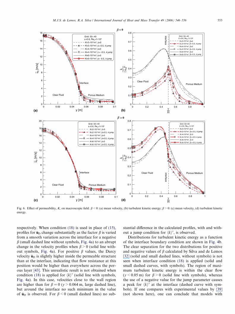
Fig. 6 shows the effect of the permeability K on both themean and statistical fields. Plots a–d follow the same con-vention described in Fig. 5. The figure indicates that thegreater the permeability, more flow crosses the porous sub-stratum located in the region 0.5 < y/H < 1 (Fig. 6a–c). Thecurves representing the statistical field in Fig. 6b–d showthat the levels of k increase with increasing K. As morefluid flows in less resistant media, more mean mechanicalenergy is transformed into turbulence increasing the overalllevel of k.

Finally, Fig. 7 investigates the effect of the value of / onthe behavior of the mean and turbulent fields, here also fol-lowing the same convention established when presentingFig. 5 (plots a–d). For the mean field (a, c), one can notethat close to y/H = 0.5 the greater the porosity, the higherthe velocity at the interface and the greater the mass flowrate closer to this region. At the center of the channel,the velocity decreases in order to keep the imposed massflow rate the same. It is interesting to observe that sincethe overall mass flow rate is forced to be constant, insteadof the overall pressure loss along the channel, an enhance-ment of the mass flow rate along the porous bed in theinterface region is compensated by a slight reduction onlocal velocities close to the wall. Fig. 7b–d shows corre-sponding curves for the behavior of the turbulent kineticenergy. Values of k present a slight reduction as / is incre-mented. Lower values for the turbulence level within theporous layer are coherent with the model of Eq. (8) forthe extra generation rate due to the porous matrix. As said,this extra Gi term (third on the right of (8)) was modeled asproportional to �uD and, inside the porous layer, the meanDarcy velocity is reduced as / increases.

Ultimately, results in Figs. 5–7 indicates that for flowswhere models with b < 0 are suitable, a smaller portionof the mean mechanical energy of the flow is converted intoturbulence. Results herein might be useful to environmen-talists and engineers analyzing important natural and engi-neering flows. Although in the porous substrate meanvelocity profiles are flatter, reducing the production ratePi, the generating mechanism Gi is proportional to �uD, in-creases the overall value of k. In the clear fluid, steeper gra-dients in the fluid layer also contributes for increasing thevalue of the turbulent kinetic energy. Then, either by Pi

in the clear fluid or by Gi in the porous layer, turbulent ki-netic energy is generated at a faster rate for positive valuesof b.

5. Concluding remarks

Numerical solutions for turbulent flow in compositechannels were obtained for different values of ReH, /, Kand b parameters. Results were compared with previouscomputations by Silva and de Lemos [32], which did not in-clude a diffusion jump for k. Inclusion of such term resulted

in qualitatively different profiles for the turbulence kineticenergy, ultimately indicating a different portion of theavailable mechanical energy that is converted into turbu-lence. Although simulations were presented for one-dimen-sional flows, the implementation herein was done fortwo-dimensional situations and carried out on a general-ized coordinate system. Future applications of the modelherein may be useful on the determining of the overallexchange rates of energy and mass transport across a inter-face between a porous medium and a clear region.

Acknowledgement

The authors are thankful to CNPq and FAPESP, Brazil,for their financial support during the course of thisresearch.

References

[1] X.Y. Zhou, J.C.F. Pereira, A multidimensional model for simulatingvegetation fire spread using a porous media sub-model, Fire Mater.24 (2000) 37–43.

[2] M.R. Hoffmann, Application of a simple space-time averaged porousmedia model to flow in densely vegetated channels, J. Porous Media 7(3) (2004) 183–191.

[3] S.N. Lane, R.J. Hardy, Porous rivers: a new way of conceptualizingand modeling river and floodplain flows? in: D. Ingham, I. Pop(Eds.), Transport Phenomena in Porous Media II, first ed., PergamonPress, 2002, pp. 425–449 [Chapter 16].

[4] M. Prithiviraj, M.J. Andrews, Three-dimensional numerical simula-tion of steel-and-tube heat exchanger. Part I—Foundation and fluidmechanics, Numer. Heat Transfer A—Appl. 33 (1998) 799–816.

[5] W.T. Sha, A new porous-media approach for thermal–hydraulicanalysis, Trans. ANS 39 (1981) 510–512.

[6] J.A. Ochoa-Tapia, S. Whitaker, Momentum transfer at the boundarybetween a porous medium and a homogeneous fluid. I—Theoreticaldevelopment, Int. J. Heat Mass Transfer 38 (1995) 2635–2646.

[7] J.A. Ochoa-Tapia, S. Whitaker, Momentum transfer at the boundarybetween a porous medium and a homogeneous fluid. II—Comparisonwith experiment, Int. J. Heat Mass Transfer 38 (1995) 2647–2655.

[8] A.V. Kuznetsov, Analytical investigation of the fluid flow in theinterface region between a porous medium and a clear fluid inchannels partially filled with a porous medium, Int. J. Heat FluidFlow 12 (1996) 269–272.

[9] A.V. Kuznetsov, Influence of the stresses jump condition at theporous-medium/clear-fluid interface on a flow at a porous wall, Int.Commun. Heat Mass Transfer 24 (1997) 401–410.

[10] A.V. Kuznetsov, Fluid mechanics and heat transfer in the interfaceregion between a porous medium and a fluid layer: a boundary layersolution, J. Porous Media 2 (3) (1999) 309–321.

[11] S. Whitaker, Advances in theory of fluid motion in porous media,Indust. Eng. Chem. 61 (1969) 14–28.

[12] W.G. Gray, P.C.Y. Lee, On the theorems for local volume averagingof multiphase system, Int. J. Multiphase Flow 3 (1977) 333–340.

[13] M.J.S. de Lemos, M.H.J. Pedras, Simulation of turbulent flowthrough hybrid porous medium-clear fluid domains, in: Proc. ofIMECE2000—ASME—Int. Mech. Eng. Congr., ASME-HTD-366-5,ISBN 0-7918-1908-6, Orlando, FL, 2000, pp. 113–122.

[14] M.H.J. Pedras, M.J.S. de Lemos, Macroscopic turbulence modelingfor incompressible flow through undeformable porous media, Int. J.Heat Mass Transfer 44 (6) (2001) 1081–1093.

[15] M.H.J. Pedras, M.J.S. de Lemos, Simulation of turbulent flow inporous media using a spatially periodic array and a low Re

556 M.J.S. de Lemos, R.A. Silva / International Journal of Heat and Mass Transfer 49 (2006) 546–556

two-equation closure, Numer. Heat Transfer A—Appl. 39 (1) (2001)35–59.

[16] M.H.J. Pedras, M.J.S. de Lemos, On mathematical description andsimulation of turbulent flow in a porous medium formed by an arrayof elliptic rods, ASME J. Fluids Eng. 123 (4) (2001) 941–947.

[17] M.H.J. Pedras, M.J.S. de Lemos, Computation of turbulent flow inporous media using a low Reynolds k–emodel and an infinite array oftransversally displaced elliptic rods, Numer. Heat Transfer A—Appl.43 (6) (2003) 585–602.

[18] M.H.J. Pedras, M.J.S. de Lemos, On volume and time averaging oftransport equations for turbulent flow in porous media, ASME-FED,vol. 248, Paper FEDSM99-7273, ISBN 0-7918-1961-2, 1999.

[19] M.H.J. Pedras, M.J.S. de Lemos, On the definition of turbulentkinetic energy for flow in porous media, Int. Commun. Heat MassTransfer 27 (2) (2000) 211–220.

[20] F.D. Rocamora Jr., M.J.S. de Lemos, Analysis of convective heattransfer for turbulent flow in saturated porous media, Int. Commun.Heat Mass Transfer 27 (6) (2000) 825–834.

[21] M.J.S. de Lemos, M.H.J. Pedras, Recent mathematical models forturbulent flow in saturated rigid porous media, ASME J. Fluids Eng.123 (4) (2001) 935–940.

[22] M.J.S. de Lemos, E.J. Braga, Modeling of turbulent naturalconvection in saturated rigid porous media, Int. Commun. HeatMass Transfer 30 (5) (2003) 615–624.

[23] M.J.S. de Lemos, M.S. Mesquita, Turbulent mass transport insaturated rigid porous media, Int. Commun. Heat Mass Transfer 30(1) (2003) 105–113.

[24] M.J.S. de Lemos, L.A. Tofaneli, Modeling of double-diffusiveturbulent natural convection in porous media, Int. J. Heat MassTransfer 47 (19–20) (2004) 4221–4231.

[25] E.J. Braga, M.J.S. de Lemos, Turbulent natural convection in aporous square cavity computed with a macroscopic k–e model, Int. J.Heat Mass Transfer 47 (26) (2004) 5639–5650.

[26] E.J. Braga, M.J.S. de Lemos, Heat transfer in enclosures having afixed amount of solid material simulated with heterogeneous andhomogeneous models, Int. J. Heat Mass Transfer 48 (23–24) (2005)4748–4765.

[27] E.J. Braga, M.J.S. de Lemos, Laminar natural convection in cavitiesfilled with circular and square rods, Int. Commun. Heat MassTransfer, in press.

[28] F.D. Rocamora Jr., M.J.S. de Lemos, Laminar recirculating flow andheat transfer in hybrid porous medium-clear fluid computationaldomains, in: Proc. of 34th ASME-National Heat Transfer Conference(on CD-ROM), ASME-HTD-I463CD, Paper NHTC2000-12317,ISBN 0-7918-1997-3, Pittsburgh, PA, 2000.

[29] F.D. Rocamora Jr., M.J.S. de Lemos, Heat transfer in suddenlyexpanded flow in a channel with porous inserts, in: Proc. ofIMECE200—ASME—Int. Mech. Eng. Congr., ASME-HTD-366-5,ISBN 0-7918-1908-6, Orlando, FL, 2000, pp. 191–195.

[30] M. Assato, M.H.J. Pedras, M.J.S. de Lemos, Numerical solution ofturbulent channel flow past a backward-facing step with a porous

insert using linear and nonlinear k–e models, J. Porous Media 8 (1)(2005) 13–29.

[31] R.A. Silva, M.J.S. de Lemos, Numerical analysis of the stress jumpinterface condition for laminar flow over a porous layer, Numer. HeatTransfer A—Appl. 43 (6) (2003) 603–617.

[32] R.A. Silva, M.J.S. de Lemos, Turbulent flow in a channel occupied bya porous layer considering the stress jump at the interface, Int. J. HeatMass Transfer 46 (26) (2003) 5113–5121.

[33] R.A. Silva, M.J.S. de Lemos, Laminar flow around a sinusoidalinterface between a porous medium and a clear fluid, in: Proc.COBEM2003—17th. Int. Congr. of Mech. Eng., Paper 1528 (on CD-ROM), Sao Paulo, Brazil, 10–14 November 2003.

[34] M.J.S. de Lemos, R.A. Silva, Turbulent flow around a wavy interfacebetween a porous medium and a clear domain, in: Proc. ASME-FEDSM2003—Fluids Engineering Division Summer Meeting, PaperFEDSM2003-45457 (on CD-ROM), Honolulu, Hawaii, USA, 6–11July 2003.

[35] A.V. Kuznetsov, L. Cheng, M. Xiong, Effects of thermal dispersionand turbulence in forced convection in a composite parallel-platechannel: investigation of constant wall heat flux and constant walltemperature cases, Numer. Heat Transfer A 42 (2002) 365.

[36] A.V. Kuznetsov, M. Xiong, Development of an engineering approachto computations of turbulent flows in composite porous/fluiddomains, Int. J. Thermal Sci. 42 (2003) 913.

[37] A.V. Kuznetsov, S.M. Becker, Effect of the interface roughness onturbulent convective heat transfer in a composite porous/fluid duct,Int. Commun. Heat Mass Transfer 31 (1) (2004) 11.

[38] A.V. Kuznetsov, Numerical modeling of turbulent flow in acomposite porous/fluid duct utilizing a two-layer k–e model toaccount for interface roughness, Int. J. Thermal Sci. 43 (11) (2004)1047–1056.

[39] P. Prinos, D. Sofialidis, E. Keramaris, Turbulent flow over and withina porous bed, J. Hydraul. Eng. 129 (9) (2003) 720–733.

[40] W.P. Breugem, B.J. Boersma, R.E. Uittenbogaard, Direct numericalsimulations of plane channel flow over a 3D cartesian grid of cubes,in: Proc. of ICAPM2004—International Conference on Applicationsof Porous Media 2004, Evora, Portugal, 24–27 May 2004, pp. 27–35.

[41] W.P. Breugem, B.J. Boersma, Direct numerical simulations ofturbulent flow over a permeable wall using a direct and a continuumapproach, Phys. Fluids 17 (2) (2005).

[42] M.J.S. de Lemos, Turbulent kinetic energy distribution across theinterface region between a porous medium and a clear fluid, in: Proc.ICTEA—Int. Conf. Thermal Eng. Theory and Applications, PaperICTEA-TF2-01, Beirut, Lebanon, 31 May–4 June 2004.

[43] M.J.S. de Lemos, Turbulent kinetic energy distribution across theinterface between a porous medium and a clear region, Int. Commun.Heat Mass Transfer 32 (1–2) (2005) 107–115.

[44] K. Lee, J.R. Howell, Forced convective and radiative transfer withina highly porous layer exposed to a turbulent external flow field, in:Proc. 1987 ASME–JSME Thermal Engineering Joint Conf., vol. 2,1987, pp. 377–386.