Numerical simulation of turbulent diffusion flames using ...
232
UPC CTTC Numerical simulation of turbulent diffusion flames using flamelet models on unstructured meshes Centre Tecnol` ogic de Transfer` encia de Calor Departament de M` aquines i Motors T` ermics Universitat Polit` ecnica de Catalunya Jordi Ventosa Molina Doctoral Thesis
-
Upload
khangminh22 -
Category
Documents
-
view
2 -
download
0
Transcript of Numerical simulation of turbulent diffusion flames using ...

UPC CTTC
Numerical simulation of turbulentdiffusion flames using flamelet
models on unstructured meshes
Centre Tecnologic de Transferencia de Calor
Departament de Maquines i Motors Termics
Universitat Politecnica de Catalunya
Jordi Ventosa MolinaDoctoral Thesis


Numerical simulation of turbulent diffusion flamesusing flamelet models on unstructured meshes
Jordi Ventosa Molina
TESI DOCTORAL
presentada al
Departament de Maquines i Motors T‘ermicsE.T.S.E.I.A.T.
Universitat Politecnica de Catalunya (UPC)
per a l’obtencio del grau de
Doctor per la Universitat Politecnica de Catalunya
Terrassa, Setembre 2015


Numerical simulation of turbulent diffusion flamesusing flamelet models on unstructured meshes
Jordi Ventosa Molina
Directors de la Tesi
Dr. Assensi Oliva Llena
Dr. Carles David Perez Segarra
Dr. Oriol Lehmkuhl Barba


Als meus pares i avis.
All right, so it’s possible there’s an alternate version of myself out therethat actually understands what the hell you’re talking about.
-Col. O’Neill (Stargate)
Asgard: Understand this: there was once an alliance of four greatraces in the galaxy. The Asgard, the Nox, the Furlings and the Ancients,the builders of the Stargates. This alliance was built over many millen-nium. Your race has much to prove before we may interact at such alevel.
O’Neill: You folks should understand that we’re out there. Now. Wemight not be ready for a lot of this stuff, but we’re doing the best we can.We are a very curious race.
Asgard: You have already taken the first steps toward becoming theFifth Race.
Stargate, The Fifth Race

vi

AgraımentsEscriure aquestes lınies implica tancar un cicle, que n’obre un de nou. Ara be,
per arribar a aquest punt hi ha hagut companys de viatge, tant a nivell profes-sional/academic com personal, als qui m’agradaria agrair l’ajuda i el suport rebuts.
En primer lloc, voldria agrair al Prof. Assensi Oliva, catedratic del Centre Tec-nologic de Transferencia de Calor (CTTC), per haver-me donat la possibilitat derealitzar el doctorat en aquest departament. Tambe pel suport i la confianca en lafeina que s’ha estat realitzant durant el doctorat.
Al Prof. Carles David Perez Segarra, catedratic del CTTC, per la seva ajudadurant el doctorat. Sobretot agrair-li l’ajuda i temps dedicat a resoldre tot tipusde questions. La seva capacitat de trobar respostes mitjancant l’analisi detallada irigurosa de les equacions descrivint el fenomen d’interes es una font d’inspiracio en lamanera de treballar.
Al Dr. Oriol Lehmkuhl, supervisor, mentor i bon amic. La feina que s’ha pogutdesenvolupar en aquesta tesi no es pot entendre sense les seves aportacions i la sevacapacitat per entendre la dinamica de fluids. La seva capacitat per entendre la mod-elitzacio de la turbulencia i les seves recomanacions i consells son altament valorats.
Apart de la vessant fısica, si avui (crec que) puc dir que se programar en C++ esper haver-ne apres del seu exemple. Al comencar el doctorat creia saber programar,aquest temps m’ha demostrat el contrari.
I would like to thank Prof. Pedro Martins Coelho for the stay at Instituto SuperiorTecnico of the Universidade Tecnica de Lisboa (IST-UTL). Furthermore, his help andanswers to my questions during my stay are highly valued.
Al Jordi Chiva li voldria agraır tota l’ajuda en la resolucio d’errors de programacioi d’optimitzacio de codi. Realment no se quantes hores de debugging m’he estalviatgracies a la seva ajuda.
Agrair al Dr. Lluis Jofre l’ajuda rebuda en el desenvolupament de la llibreriade propietats fısiques. Tambe per algunes discussions forca interessants i per haverestat una mica de guia durant el doctorat, ja que el va comencar un any abans.Tambe mencionar l’Aleix Baez, amb el qual vam desenvolupar una llibreria per avaluartermes convectius i difusius. Ambdues llibreries son centrals per aquesta tesi i arason usades ampliament en el grup. Tampoc voldria oblidar-me d’en Jordi Muela, elqual ha col·laborat en desenvolupar i millorar diferents aspectes dels algoritmes percombustio.
Donada la naturalesa computacional de la tesi, no voldria oblidar-me els in-formatics del grup, passats i actuals, en Dani, el Gabriel, l’Octavi i el Ramiro, perl’ajuda en aspectes de software i hardware. No voldria deixar-me gent del CTTC,com la Roser Capdevila, die Deutschmitschulerin, el Joan Farnos, l’Hector Giraldez,
vii

viii Agraıments
i Ricard Borrel, i els professors Joaquim Rigola, Carles Oliet i Ivette Rodrıguez.
En l’ambit mes personal, voldria fer una mencio a tota la colla d’amics de Reus.En part no he acabat del tot ”mentally lost” pels bons moments compartits. I aaquelles noves persones que en un moment apareixen i et canvien.
Finalment, no puc deixar d’agraır a la meva familia tot el suport rebut. Especial-ment al meu pare Joan i la meva mare Carme, per ser-hi sempre i ajudar-me a creixercom a persona. Als meus avis, Jaime, Trinidad, Joan i Pepita pels valors que m’hantransmes. I tambe es mereix una mencio especial la meva germana Gloria, tot i quemolt sovint siguem com gat i gos.
Jordi V. M.

AbstractCombustion is a temporal and spatial multiscale problem characterised by the
interaction between chemical reactions and turbulent flow. Furthermore, chemicalreactions involve a large number of participating species. Hence, models are requiredto reduce the dimensionality of the problem. In addition, turbulence is a complexprocess by itself, whose resolution is computationally demanding and still is a topicof current research. Therefore, modelling is also applied to reduce its computationaleffort.
The present thesis aims at developing numerical methods and algorithms for theefficient simulation of diffusion flames in the flamelet regime. To tackle turbulentchemically reacting flows a double framework is used in the present thesis. On theone hand, flow description is performed in the context of Large Eddy Simulation(LES) techniques. In LES, by spatially filtering the Navier-Stokes equations, thelarge scales of the flow are solved and the small scales are modelled, as they present amore universal behaviour. On the other hand, thermochemistry is modelled by meansof flamelet models. Chemical reactions occur at the molecular level. Consequently,in many cases of academic and industrial interest, reactions occur at scales smallerthan the smallest flow scale, namely the Kolmogorov scale. With this assumption, theflamelet regime is characterised by the split of the combustion process into a flamestructure case and flow transport case.
Therefore, to study chemically reacting flows different models and algorithms arerequired. First, an algorithm for computing variable density flows. Second, a model todescribe chemical kinetics. Finally, a procedure to link the transport model with theflame model. In order to accomplish these goals the thesis is divided into five chapters,each one describing and analysing a specific aspect of the required numerical methods.
In first place, in Chapter 1 the basic formulation for describing chemically reactingflows is detailed. Chemical kinetics are briefly described and transport terms formulticomponent flows are detailed. Then, an introduction to turbulent combustionis performed, where the challenges of simulating these flows using finite rate kineticsare stated. It is then argued that specific models are required.
Before proceeding to describe the combustion model, an algorithm for the simu-lation of variable density flows is described and studied in Chapter 2. Furthermore,the study revolves around the use of unstructured meshes, since one of the focus ofthe thesis is the capacity of the developed numerical methodology to be applied oncomplex geometries. A temporal integration scheme, specifically a multi-step scheme,and two spatial discretisation schemes, namely collocated and staggered schemes, aredescribed and studied. Reacting and non-reacting test cases are considered.
In Chapter 3 a flamelet model for the simulation of diffusion flames is described.First, the flamelet regime is described and the flame equations in composition space,
ix

x Abstract
or mixture fraction space, are presented. Then, a Flamelet/Progress-Variable modelis used to fully describe the flame in mixture fraction space. The two main param-eters used are the mixture fraction and the progress-variable. Additionally, a finitedifferences method for the solution of the flamelet equations is presented. Since thetarget flames are turbulent, assumed probability density functions are introduced inorder to restate the flamelet solutions as stochastic quantities. The model allows pre-computing the flame thermochemistry and storing it into a database, which is thenaccessed during simulations in physical space.
The next two chapters deal with the parameters used to represent the flameletdatabase. In first place, Chapter 4 studies the definition of the progress-variable,which is required to unambiguously represent the chemical state. This statementmainly translates into a requirement of monotonic evolution. The definition of thisparameter has been reported to be case sensitive. The present work evidences a depen-dence on the diffusion model. Definitions found valid for Fickian diffusion are shownto result in non-monotonic distributions when differential diffusion is considered. Fur-thermore, in the chapter two detailed chemical mechanism are considered. Tests in-clude a methane/hydrogen/nitrogen diffusion flame and a self-igniting methane flame,where the fuel issues into a vitiated coflow. In the latter case, chemical mechanismsare shown to play a central role in the prediction of the flame stabilisation distance.
Lastly, when turbulent flames are considered, the flamelet database is stated asa function of stochastic parameters. Among them, the mixture fraction variance,which represents mixing at the subgrid level, is not directly computed and requiresmodelling. Since chemical reactions in the flamelet regime occur at scales smallerthan the Kolmogorov scale, the correct characterisation of subgrid mixing is a criticalissue. Hence, in Chapter 5 different models for the evaluation of the subgrid varianceare studied. The study case is the methane/hydrogen/nitrogen diffusion flame. Thestudy shows that correct description of the subgrid mixing is critical in accuratelypredicting the flame stabilisation.

Contents
Agraıments vii
Abstract ix
1 Introduction 11.1 Prologue . . . . . . . . . . . . . . . . . . . . . . . . . . . . . . . . . . . 11.2 Combustion modelling . . . . . . . . . . . . . . . . . . . . . . . . . . . 3
1.2.1 Chemical kinetics . . . . . . . . . . . . . . . . . . . . . . . . . . 41.2.2 Transport equations . . . . . . . . . . . . . . . . . . . . . . . . 51.2.3 Burning mode . . . . . . . . . . . . . . . . . . . . . . . . . . . 101.2.4 Turbulence . . . . . . . . . . . . . . . . . . . . . . . . . . . . . 111.2.5 LES . . . . . . . . . . . . . . . . . . . . . . . . . . . . . . . . . 121.2.6 Combustion closure . . . . . . . . . . . . . . . . . . . . . . . . 14
1.3 Background at the CTTC . . . . . . . . . . . . . . . . . . . . . . . . . 171.4 Objectives . . . . . . . . . . . . . . . . . . . . . . . . . . . . . . . . . . 191.5 Outline of the thesis . . . . . . . . . . . . . . . . . . . . . . . . . . . . 21References . . . . . . . . . . . . . . . . . . . . . . . . . . . . . . . . . . . . . 22
2 Numerical assessment of conservative unstructured discretisationsfor Low-Mach flows 272.1 Introduction . . . . . . . . . . . . . . . . . . . . . . . . . . . . . . . . . 282.2 Low-Mach number equations . . . . . . . . . . . . . . . . . . . . . . . 30
2.2.1 Chemically reacting flows . . . . . . . . . . . . . . . . . . . . . 312.2.2 Thermodynamic pressure . . . . . . . . . . . . . . . . . . . . . 322.2.3 Momentum projection scheme - Fractional Step method . . . . 33
2.3 Unstructured discretisation . . . . . . . . . . . . . . . . . . . . . . . . 342.3.1 Collocated discretisation: . . . . . . . . . . . . . . . . . . . . . 362.3.2 Staggered discretisation: . . . . . . . . . . . . . . . . . . . . . 372.3.3 Face interpolation schemes . . . . . . . . . . . . . . . . . . . . 402.3.4 Boundaries . . . . . . . . . . . . . . . . . . . . . . . . . . . . . 42
2.4 Temporal Integration Algorithm . . . . . . . . . . . . . . . . . . . . . 422.4.1 Temporal integration algorithm . . . . . . . . . . . . . . . . . . 43
2.5 Numerical Tests . . . . . . . . . . . . . . . . . . . . . . . . . . . . . . . 452.5.1 Test Case 1 - Interpolation schemes accuracy . . . . . . . . . . 462.5.2 Test Case 2 - Analysis of the spatial discretisations . . . . . . . 482.5.3 Test Case 3 - Analysis of the transient behaviour . . . . . . . . 53
2.6 Conclusions . . . . . . . . . . . . . . . . . . . . . . . . . . . . . . . . . 56
xi

xii Contents
References . . . . . . . . . . . . . . . . . . . . . . . . . . . . . . . . . . . . . 58
3 Flamelet modelling of nonpremixed combustion phenomena 633.1 Introduction . . . . . . . . . . . . . . . . . . . . . . . . . . . . . . . . . 643.2 Flamelet model . . . . . . . . . . . . . . . . . . . . . . . . . . . . . . . 65
3.2.1 Classical Flamelet . . . . . . . . . . . . . . . . . . . . . . . . . 723.2.2 Flamelet/Progress-variable (FPV) model . . . . . . . . . . . . 75
3.3 Flamelet database . . . . . . . . . . . . . . . . . . . . . . . . . . . . . 813.3.1 Solution of the flamelet equations . . . . . . . . . . . . . . . . . 813.3.2 Flamelet solutions . . . . . . . . . . . . . . . . . . . . . . . . . 90
3.4 Flamelets in turbulent flows . . . . . . . . . . . . . . . . . . . . . . . . 903.4.1 Radiation and NOx in turbulent flows . . . . . . . . . . . . . . 98
3.5 Database for CFD . . . . . . . . . . . . . . . . . . . . . . . . . . . . . 993.6 Concluding remarks . . . . . . . . . . . . . . . . . . . . . . . . . . . . 103References . . . . . . . . . . . . . . . . . . . . . . . . . . . . . . . . . . . . . 106
4 Differential diffusion effects in the progress-variable definition forFlamelet/Progress-variable models for non-premixed flames 1114.1 Introduction . . . . . . . . . . . . . . . . . . . . . . . . . . . . . . . . . 1134.2 Mathematical model . . . . . . . . . . . . . . . . . . . . . . . . . . . . 115
4.2.1 Flamelet/Progress-variable (FPV) model . . . . . . . . . . . . 1184.2.2 Numerical method . . . . . . . . . . . . . . . . . . . . . . . . . 123
4.3 Turbulent diffusion CH4/H2/N2 flame - DLR A flame . . . . . . . . . 1244.3.1 Flamelet burning region - Fickian vs Differential . . . . . . . . 1254.3.2 Progress-variable definition - steady . . . . . . . . . . . . . . . 1254.3.3 Progress-variable definition - unsteady . . . . . . . . . . . . . . 1294.3.4 Progress-variable definition - radiation . . . . . . . . . . . . . . 1324.3.5 CFD analysis . . . . . . . . . . . . . . . . . . . . . . . . . . . . 137
4.4 Turbulent auto-igniting diffusion CH4 flame - Cabra flame . . . . . . . 1424.4.1 S-shaped curve . . . . . . . . . . . . . . . . . . . . . . . . . . . 1434.4.2 Progress-variable definition . . . . . . . . . . . . . . . . . . . . 1464.4.3 CFD analysis . . . . . . . . . . . . . . . . . . . . . . . . . . . . 150
4.5 Conclusions . . . . . . . . . . . . . . . . . . . . . . . . . . . . . . . . . 154References . . . . . . . . . . . . . . . . . . . . . . . . . . . . . . . . . . . . . 156
5 Large Eddy Simulation of a shear stabilised turbulent diffusion flameusing a Flamelet/Progress-Variable model. 1615.1 Introduction . . . . . . . . . . . . . . . . . . . . . . . . . . . . . . . . . 1635.2 Mathematical model . . . . . . . . . . . . . . . . . . . . . . . . . . . . 166
5.2.1 LES model . . . . . . . . . . . . . . . . . . . . . . . . . . . . . 1665.2.2 Flamelet/Progress-Variable (FPV) model . . . . . . . . . . . . 166

Contents xiii
5.2.3 Numerical method . . . . . . . . . . . . . . . . . . . . . . . . . 1735.3 Turbulent diffusion CH4/H2/N2 flame - DLR A flame . . . . . . . . . 1735.4 Results and discussion . . . . . . . . . . . . . . . . . . . . . . . . . . . 174
5.4.1 Turbulent fluxes closure . . . . . . . . . . . . . . . . . . . . . . 1745.4.2 Flame stabilisation . . . . . . . . . . . . . . . . . . . . . . . . . 1765.4.3 Effect of the subgrid mixing closures . . . . . . . . . . . . . . . 179
5.5 Conclusions . . . . . . . . . . . . . . . . . . . . . . . . . . . . . . . . . 193References . . . . . . . . . . . . . . . . . . . . . . . . . . . . . . . . . . . . . 195
6 Conclusions 201References . . . . . . . . . . . . . . . . . . . . . . . . . . . . . . . . . . . . . 208
A Projection method in the Fractional Step for Low Mach algorithms211
B A note on software development 213References . . . . . . . . . . . . . . . . . . . . . . . . . . . . . . . . . . . . . 214
C Main publications in the context of this thesis 215

xiv Contents

1
Introduction
1.1 Prologue
From the early times of humankind fire has played a significant role in the devel-opment of human society; from its early use as a source of light and heat, and to cookfood, thus reducing the amount of energy used in digesting it, up to modern chemicalrockets, gas turbines and internal combustion engines. Not only has it been used toprogress but also has been an element of destruction. Moreover, the influence of firein human culture goes beyond that of practical use. In many mythological stories,fairy-tales and different sorts of artistic representations fire is a central element. Ithas been used as a symbol for both creation and destruction, which also has beeninterpreted as a purification process.
Besides philosophical considerations, fire, or specifically combustion, has been atthe centre of human life. It has been the main energy source during centuries. Al-though in the last century several new technologies, like nuclear energy and renewableenergies, such as solar and wind power, have gained, or are gaining, notoriety, combus-tion driven machinery still plays a significant role in the amount of produced energyin the world. Furthermore, it is forecast that at least in the following 50 to 80 years,combustion generated energy will still be one of the main energy sources worldwide.Besides, there are other processes related to combustion which are not directly linkedto energy generation but are linked to human safety, such as fires in wildland and inbuildings. Moreover, in combustion processes, in addition to the energy release, thereis a generation of non-desired products, or pollutants. In the last decades, regulationson pollutants is becoming more stringent due to concerns on the effect on humanhealth and on the environment. These pollutants are usually in lower proportionscompared to the main combustion products and their dynamics are usually different.Therefore, accurate models are required to correctly characterise pollutant emissions.Then, methods and techniques must be developed in order to reduce their production.Hence, there is a need for understanding how pollutants are created and transported.
Combustion is a conglomeration of different complex processes which interact and
1

2 Chapter 1. Introduction
result in a, usually visible, exothermic process. Beginning with the core process,chemical reactions describe how certain reactants, usually a pair of fuel and oxidizer,combine and produce certain products while releasing heat. Then, reactants may befound in different states: as solid fuel, in a liquid bed or spray, or in gas form. Theformer two require that, prior to combustion, a phase change to the gas state musttake place. Concerning the combustion products, they are usually in gas form, sincechemical heat released causes a large temperature increase. This last effect introducestwo critical aspects of combustion processes, heat transfer and radiation. The formerrequires describing how heat is transported within a flow field composed of differentelements, or species. The latter effect, radiation, is a complex phenomenon by itself,which, due to the coupling with the other described phenomena, becomes even morechallenging. A last aspect to remark is that in most designs of technological inter-est, flows are usually turbulent, mainly due to the increased power output, comparedto laminar designs. Turbulence, which lies at the heart of the Navier-Stokes equa-tions, is a challenge which as of today is still unclosed and is considered one of theseven “Millennium problems”, set by the Clay Mathematics Institute [1]. Hence, thecombination of chemistry, heat and mass transfer, turbulence, phase change and ra-diation, among others, pose a significant challenge that requires advanced modellingtechniques in order to obtain accurate solutions with finite resources.
Initial works in the combustion field date back to the end of the 19th centuryby LeChatelier and Arrhenius and in the thirties of the 20th century by Burke-Schumman, among others. Following, during the 20th century the number of studiesfocused on combustion increased. It was soon realised that the complexity of theinvestigated phenomena required the use of specific models which would reduce thenumber of unknowns and interactions. In the process, combustion researchers iden-tified canonical situations with different characteristic behaviours, based on whetherthe reactants are mixed prior to combustion or not: premixed and non-premixedflames. Initially, fundamental analysis of flames in either regime were mostly basedon one-dimensional configurations. For diffusion flames, most models resorted to aflame in a counterflow configuration, where each reactant issues from one differentinlet, and the reaction zone separates each stream. For premixed flames, the alreadymixed reactants undergo a temperature increase while going through a thin reactionzone, where the flame front displaces with a characteristic speed, the laminar flamespeed.
The extension to turbulent flames proved challenging due to the coupling betweenchemistry and turbulence. The challenges found in laminar flames grow significantlywhen considering turbulent motions. Hence, most models developed for turbulentflames were based on what had been learned from laminar flames. Phenomenologicalmodels allowed solving certain cases with good accuracy.
Parallel to the increase in computer power during the 20th century, the capabilities

1.2. Combustion modelling 3
for numerical simulations of fluid flow increased, and also for combustion. Thanks tothis computational power increase, Computational Fluid Dynamics (CFD) emergedas a tool to solve the Navier-Stokes equations numerically. An aspect to bear in mindconcerning the research in the combustion field is that performing experimental mea-surements is specially challenging due to the high temperatures involved and the largenumber of participating species. Hence, CFD can provide a good understanding ofthe processes, although the modelling effort is important. However, a large effort wasand still is needed to solve these equations. Nonetheless, the information gatheredusing these techniques has proven invaluable in understanding the laws controlling thephysics of flow movement and transport. In recent years, the computational capacityand understanding of combustion processes has allowed researchers and engineers totackle complex engineering designs such as the combustion process within an aero-nautical gas turbine [2–4].
In the following an introduction to the mathematical description of combustionphenomena is presented. Chemistry, transport equations and coefficients are describedfor the general solution of flames. The extension to turbulent flows is considered anddifferent models are discussed. The following discussion is not intended as an extensivestate of the art, rather as an introduction and basis for the rest of the thesis. In eachchapter a specific state of the art is conducted.
1.2 Combustion modelling
A combustion process is an exothermic chemical reaction taking place within afluid flow. Therefore, its study requires describing a chemical process and the move-ment of the flow. The chemical composition of a mixture composed of N species isdescribed by means of the species mass fractions Yk = mk/m, where mk and m arethe kth-species and mixture mass respectively, both in a given volume. The densityof the mixture ρ, linked to pressure P and temperature T , is evaluated through theideal gas state law
Po = ρRgT = ρR
WT = ρTR
N∑k=1
YkWk
(1.1)
where Rg and R = 8.314J/(Kmol) are the specific and ideal gas constants, respec-tively. The mixture molar mass W is calculated from the species molar masses Wk
1
W=
N∑k=1
YkWk
(1.2)

4 Chapter 1. Introduction
Mass fractions are related to molar fractions Xk and molar concentrations [Xk]through the molar mass
Xk =W
WkYk (1.3)
[Xk] = ρYkWk
= ρXk
W(1.4)
The thermodynamic state of the mixture can be represented by the enthalpy h,defined as the sum of its chemical and sensible parts
h =
N∑k=1
Ykhk =
N∑k=1
Yk
(∆hof,k︸ ︷︷ ︸chemical
+
∫ T
T0
cpk(T )dT︸ ︷︷ ︸sensible
)(1.5)
where hk is a species enthalpy, ∆hof,k is a species enthalpy of formation, cpk is aspecies heat capacity and T0 = 298.2K is the reference temperature for evaluatingthermodynamic data. Both enthalpy and heat capacity of each species are calculatedusing NASA’s polynomials [5, 6] and the mixture heat capacity cp and enthalpy h areevaluated as
cp(T ) =
N∑k=1
Ykcpk(T ) (1.6)
h(T ) =
N∑k=1
Ykhk(T ) (1.7)
1.2.1 Chemical kinetics
A chemical process is a series of interactions involving N different chemical speciesand is represented by Nr reactions
N∑k=1
ν′r,kYk N∑k=1
ν′′r,kYk r = 1...Nr (1.8)
where Yk represents the species involved in reaction r, ν′r,k and ν′′r,k are the molarstoichiometric coefficients of the kth species in reaction r. The reaction rate for eachequation is given by the empirical rate law
wk,r = Wkνr,kRr (1.9)
where νr,k = ν′′r,k − ν′r,k and Rr is the rate of progress of reaction r given by
Rr = kfr
N∏k=1
[Xk]ν′r,k − kbr
N∏k=1
[Xk]ν′′r,k (1.10)

1.2. Combustion modelling 5
where kfr and kbr are the forward and backward kinetic rate constants, which are notconstant in the strict sense. Forward rate constants are evaluated using Arrheniuslaw
kfr = AT βexp(−Ea,rRT
)(1.11)
where A is the pre-exponential constant, β the temperature exponential and Ea,r =RTa,r is the activation energy, which can be related to an activation temperatureTa,r. Chemical mechanisms containing sets of reactions and values for these constantscan be found in the literature; ranging from detailed mechanisms, such as the GRImechanism [7] for methane combustion, to reduced mechanisms, for example theJones and Lindstedt mechanism for methane [8] or the mechanism of Mueller et al.for hydrogen [9], and single-step irreversible mechanisms. Backward constants areusually not included, but are computed through reaction equilibrium constants
kbr =kfr(
paRT
)∑Nk=1 νr,kexp
(∆S0
k
R − ∆H0k
RT
) (1.12)
where pa = 0.1MPa and ∆S0k and ∆H0
k the standard entropy and enthalpy changesfor reaction r.
The reaction rate for any species is then
wk = Wk
Nr∑r=1
νr,kRr (1.13)
Summing all reactions rates of all species results in
N∑k=1
wk =
N∑k=1
Wk
( Nr∑r=1
νr,kRr)
=
Nr∑r=1
Rr( N∑k=1
Wkνr,k
)= 0 (1.14)
since∑Nk=1Wkνr,k = 0 which shows that mass is conserved.
1.2.2 Transport equations
The Navier-Stokes equations can describe a combustion process taking place withina fluid flow. Depending on the characteristic Mach number of the flow, either lowMach formulations or compressible formulations are used to describe the fluid flow.In the current thesis, the study is focused on combustion in low Mach flows. Solvinga non-reacting case involves computing six variables, density, pressure, velocity andtemperature, whereas a reacting case adds N more variables. Hence, the computationof reacting cases first entails an increment of the computational effort. In the follow-ing it will also be shown that the modelling effort is also increased. The governing

6 Chapter 1. Introduction
equations, which are presented in detail in Chapter 2 are
∂ρ
∂t+∂ρuj∂xj
= 0 (1.15)
∂ρui∂t
+∂ρujui∂xj
= − ∂p
∂xi+∂τij∂xj
+ ρgi (i = 1, 2, 3) (1.16)
∂ρh
∂t+∂ρujh
∂xj=dPodt
+ vi∂pi∂xi− qR − ∂qj
∂xj+ τij
∂ui∂xj
(1.17)
∂ρYk∂t
+∂ρujYk∂xj
= −∂jk,j∂xj
+ wk (k = 1..N) (1.18)
where t represents time, ρ the fluid density, u a mixture averaged velocity, τ the shearstress tensor, g the gravity, h the specific enthalpy of the mixture, qj the diffusionheat flux, qR the radiant heat rate, Yk a species mass fraction, wk a species reactionrate and jk = ρVk,jYk a species diffusion mass flux, where the diffusion flux is definedthrough a diffusion velocity Vk,j . For low Mach flows, the pressure can be split intoa hydrodynamic pressure p and a thermodynamic pressure Po. This set of equationsinvolve several transport terms to be modelled, i.e. the shear stress tensor τij , theheat flux qj and the mass fluxes jk,j .
Momentum equationIn the momentum equation Eq. (1.16) the shear stress tensor is modelled throughStoke’s law for Newtonian fluids
τij = µ
(∂ui∂xj
+∂uj∂xi− 2
3δij∂uk∂xk
)(1.19)
where δij is the Kronecker Delta and µ is the mixture dynamic viscosity.
Energy equationHeat diffusion in multicomponent flows takes place through two mechanisms, thermalheat diffusion described by Fourier’s law and heat transport by inter-diffusion ofspecies with different enthalpies
qj = −κ ∂T∂xj
+
N∑k=1
hkjk,j (1.20)
where κ is the mixture thermal conductivity. A further term that could be consideredis the flux of energy produced by concentration gradients, namely the Duffour effect.This effect is based on Onsager’s reciprocal relations of irreversible thermodynamics.It implies that if temperature gradients give rise to diffusion velocities (thermal dif-fusion), then concentration gradients must produce a heat flux. However, compared

1.2. Combustion modelling 7
to the other two terms, the Duffour contribution to the heat flux is small. Thus, ithas been neglected in the computations.
Species mass fractionMass fluxes appear in both energy and mass transport equations. Furthermore, theirproper definition is critical for conserving mass even at the differential level, since thesummation of all species transport equations must add to the continuity equation.Therefore, summing all species equations Eq. (1.18)
N∑k=1
(∂ρYk∂t
+∂ρujYk∂xj
)=
N∑k=1
(−∂jk,j∂xj
)+
N∑k=1
(wk)
(1.21)
The first two terms in the left hand side add to the continuity equation, since ρk =ρYk →
∑Nk=1 ρYk = ρ and all mass fraction add to one. Additionally, it has been
shown that the summation of all species reaction terms adds to null. Hence, all massdiffusion fluxes summed must cancel out
N∑k=1
(−∂jk,j∂xj
)= 0 (1.22)
A detailed model for diffusion velocities and fluxes can be computed from thekinetic theory [2, 10], which under some approximations reduces to the Stefan-Maxwellequation
∂Xk
∂xj=
N∑α=1
XαXk
Dαk(Vk,j − Vα,j) (1.23)
where Dαk is the binary mass diffusivity of species α into species k. Solution ofthis equation is computationally expensive [2]. Therefore, simplified models havebeen proposed: Fick’s law and Hirschfelder and Curtiss approximation. Under theassumption of equal diffusivities for all species, Fick’s law is an exact solution toEq. (1.23). Diffusion fluxes are evaluted as
jk,j = −ρD∂Yk∂xj
(1.24)
where mass diffusivity D = Dαk is equal for all species. When the equal diffusivitiesassumption is not made, diffusion fluxes are evaluated using Hirschfelder and Curtissapproximation [2], which is a first order approximation to Eq. (1.23)
Vk,jXk = −Dk∂Xk
∂xj−→ Vk,jYk = −Dk
Wk
W
∂Xk
∂xj(1.25)

8 Chapter 1. Introduction
where Eq. (1.3) has been used to convert molar fractions into mass fractions. However,this approximation does not conserve mass. If Eq. (1.22) is evaluated using Eq. (1.25)to describe the species mass fluxes, there remains a residual. In order to ensure massconservation, a correction velocity V cj is introduced to the Hirschfelder and Curtissdiffusion velocity
V cj =
N∑k=1
DkWk
W
∂Xk
∂xj(1.26)
Vk,jYk = −DkWk
W
∂Xk
∂xj+ V cj (1.27)
This approach can be shown to be equivalent to Fick’s law when equal diffusivitiesare assumed.
As a last remark, the Soret effect has been neglected in the mass transport equa-tion. Similar to the energy equation, but with opposite effect, the Soret effect is themass diffusion due to thermal gradients.
Transport coefficientsThe molecular fluxes for momentum τij , heat qj and mass jk,j require the com-
putation of mixture molecular transport coefficients, which in turn depend on thespecies molecular transport coefficients.
For the mixture averaged dynamic viscosity µ the semi-empirical formula by Bird[11] has been used
µ =
N∑k=1
Xkµk∑Nα=1XαΦkα
(1.28a)
Φkα =1√8
(1 +
Wk
Wα
)−1/2(1 +
(µkµα
)1/2(Wα
Wk
)−1/4)2
(1.28b)
where µk are binary dynamic viscosities. Mixture and species thermal conductivities,κ and κk respectively, are evaluated using the same set of equations, using κ insteadof µ where appropriate. For cases where the viscosity is not required, a simplerexpression can be used to estimate the thermal conductivity [12] with an error of afew percent [13]
κ =1
2
(N∑k=1
Xkκk +
(N∑k=1
Xk
κk
)−1)(1.29)
The exact description of mass diffusion involves solving the Stefan-Maxwell equa-tion with the evaluation of binary diffusivities. However, as stated this process is too

1.2. Combustion modelling 9
computationally demanding. Hence, when the Hirschfelder and Curtiss approxima-tion is used with multicomponent diffusivities, a diffusivity of each species into themixture is evaluated. The multicomponent mass diffusivity is estimated [2] through
Dk,m = Dk =1− Yk∑Nα=1α6=k
XαDkα
(1.30)
where the subindex m indicating diffusion towards the mixture is dropped for thesake of readability, and Dk,α is the binary diffusivity.
Non-dimensional analysisEvaluation of mixture properties can still involve a significant task, even with
the simplifications just described. The non-dimensional analysis of the flame revealsseveral non-dimensional numbers relating the different transport properties. TheLewis number relates mass and heat transport
Lek =κ/ρcp
Dk, (1.31)
the Prandtl number relates momentum and heat transfer
Pr =µ/ρκ/ρcp
(1.32)
and the Schmidt number compares momentum and mass diffusion
Sck =µ/ρ
Dk(1.33)
According to [2], the Lewis number variation for each species is small through theflame front. Hence, assuming a constant Lewis number for each species and defininga suitable expression for the thermal conductivity may be adequate for simplifiedanalysis. Nonetheless, Giacomazzi et al. [14] reported that the assumption of con-stant Schmidt numbers was better suited due to the narrower distribution of Schmidtnumbers against temperature compared to the Lewis numbers.
Two further non-dimensional numbers of interest are the Reynolds number andthe Damkohler number. The former compares inertial forces to viscous forces and isdefined as
Re =ρvL
µ(1.34)
where v is a characteristic velocity of the case of study, and L is a characteristiclength. In the present thesis, jet flames are studied and the reference values usuallytaken are the fuel jet bulk velocity and the fuel jet nozzle diameter.

10 Chapter 1. Introduction
The Damkohler number compares chemical time-scales τch with transport time-scales τf , either through convection or diffusion,
Da =τfτch
(1.35)
Thermal radiationHeat transfer by radiation appears in the energy conservation equation Eq. (1.17)
through the divergence of the radiant heat flux qR. Its evaluation involves solvingfor the Radiation Transfer Equation (RTE), which describes the transfer of radiantenergy in a participating medium. The RTE is an integro-differential equation withseven independent variables: three spatial coordinates, two angular coordinates, whichdefine the direction of propagation, one spectral variable, and time. However, sinceradiation beams travel at the speed of light in the medium, the time coordinate isusually negligible in most applications [15]. Still, solving the RTE is an expensivetask. Furthermore, the complexity is increased by the need of evaluating the mediumradiative properties.
Different models have been presented in the literature to solve the RTE. Amongthem, the Discrete Ordinates Method (DOM), the Finite Volume Method (FVM) orMonte Carlo methods [16–19] are well established. Simplified methods can be appliedwhen the medium is considered optically thin. Hence, the flame has an unimpededview of the surroundings. Furthermore, self-absorption is assumed negligible com-pared to emission in the Optically Thin Method (OTM) [20, 21]. Thus, the radiationflux is modelled as a heat loss at each control volume
qR = 4σ
(T 4
N∑k=1
(pkkPk)− T 4s
N∑k=1
(pkkIk)
)(1.36)
where σ is the Stefan-Boltzmann constant, pk is the partial pressure of the kth species,kPk and kIk are the Planck-mean and incident-mean absorption coefficients, and Tsis the background temperature. Absorption coefficients obtained from RADCAL [22]were fitted to polynomials of the temperature. The radiant species considered areCO2, H2O, CH4 and CO.
This approach is significantly less expensive than the other cited methods and willbe used in this thesis.
1.2.3 Burning mode
The mathematical framework described can be used to represent most flame con-figurations. For chemical reactions to take place, reactants have to be mixed at themolecular level with enough energy for chemical reactions to start. Hence, flamedynamics are controlled through two mechanisms, the mixing rate and chemical ki-

1.2. Combustion modelling 11
netics. Depending on which mechanism is the rate controlling, two different canonicalburning modes are found.
On the one hand, in premixed flames reactants are mixed at the molecular levelbefore arriving at the flame front. Hence, chemistry is the rate controlling mechanism.Premixed flames are more intense and pollute less because the burning conditions canbe more accurately controlled through the inlet ratio of fuel and oxidant. However,their operation is dangerous since an increase of temperature at any point in thereactant stream can lead to uncontrolled ignition.
On the other hand, in diffusion flames reactants mix in the same region where theflame is located. Hence, depending on the Damkohler number, either the mixing rateor the reaction rate will be the limiting mechanism. Nevertheless, it is usually foundthat chemistry time-scales are much shorter than flow time-scales. Therefore, mixingis rate controlling. In this mode, fuel and oxidizer usually enter the combustion regionthrough separated streams. This leads to lower reaction rates, but also to highertemperatures, since reactions take place at their most suitable conditions, namely atthe stoichiometric mixture fraction. Flames in this regime are safer to operate sincereactants are not mixed until they reach the reaction zone. The current thesis isfocused on diffusion flames.
1.2.4 Turbulence
In order to increase the thermal power output of diffusion flames, it is necessaryto increase the mixing rate, since mixing is mainly the rate controlling mechanism.Hence, most applications of interest feature turbulent flows. However, turbulenceadds another layer of complexity to the description of the flow. Turbulent flowsare characterised by being transient, three-dimensional, random and involving a largenumber of temporal and spatial scales [23]. The characterisation of turbulent motionsis performed through three different strategies.
The most detailed technique, and also the most computationally demanding, is theDirect Numerical Simulation (DNS) of the flow. With this technique, all flow scalesof the Navier-Stokes equations are solved, without any model for turbulent motions1.This approach allows to fully characterise the flows of interest and obtain a detailedinformation of the physical phenomena. The large computational resources requiredmade this approach unfeasible. However, with the advent of High Performance Com-puting (HPC), this technique is becoming more affordable. Still, nowadays is mostlyrestricted to academic cases.
Turbulence modelling is required for most practical situations. Two techniquesare most commonly used, Reynolds-Averaged Navier Stokes (RANS) and Large EddySimulations (LES). In both cases the Navier-Stokes equations are filtered and tur-
1Note that models for other physical phenomena can still be introduced, for example for radiation,combustion, multiphase flows, etc.

12 Chapter 1. Introduction
bulence models are introduced. RANS techniques perform a temporal filtering, oraveraging, whereas in LES the filtering operation is performed spatially. This filter-ing operation has different implications. In RANS all scales of the energy spectrum aremodelled, whereas in LES a split between resolved and unresolved scales is introducedand only the latter require modelling.
Focusing on RANS techniques, it is based on a splitting where variables φ are de-composed into an average φ and a fluctuating part φ′, with φ = φ+ φ′. The methodsolved for mean quantities of all variables. Models are required to close the Reynoldsstress tensor and evaluate the chemical source term and heat of reaction. Althoughthe models required are found to be case dependent and sensitive to the model pa-rameters, the technique offers an affordable approach to many cases of academic andindustrial relevance. It is still nowadays used in many fields as the standard approach.Nonetheless, since solution variables are temporally averaged quantities, the methodstruggles with transient phenomena. In combustion, ignition and extinction events orinstabilities are an example of these shortcomings, among others.
Regarding LES, the method splits the different quantities of interest into a resolvedand an unresolved part. The former are explicitly solved during CFD simulations,whereas the latter are modelled. The advantage of this approach, is that the behaviourof the flow small scales is found to be more universal [24, 25]. Hence, more generalmodels can be proposed. Although less computationally demanding than DNS simu-lations, the increase with respect to RANS simulations is considerable. Nonetheless,this technique allows characterising transient events and similar phenomena. In thepresent thesis studies are carried out under an LES framework. Further details aregiven in the following.
1.2.5 LES
Large Eddy Simulation describes the motion of the large scales of the flow, whereasthe small scales are modelled. Scale splitting is performed by means of a low-passfilter,
ρφ =
∫Ω
ρφG(x, ξ)dξ (1.37)
In grid based, implicit filtering, the filter kernel G(x, ξ) becomes a top-hat filter withsize ∆ = (hi)
1/3, where hi is the mesh spacing in the i -direction. Additionally, forvariable density flows, the filtered quantities are density weighted, or Favre filtered.Favre filtered quantities can be related to Reynolds filtered quantities through
ρφ = ρφ (1.38)
Therefore, applying the filtering operation to the low-Mach Navier-stokes equa-

1.2. Combustion modelling 13
tions, they become
∂ρ
∂t+∂ρuj∂xj
= 0 (1.39)
∂ρui∂t
+∂ρuj ui∂xj
= − ∂p
∂xi+
∂
∂xj
(τij − ρu′′j u′′i
)+ ρgi (1.40)
∂ρh
∂t+∂ρuj h
∂xj=dPodt− 1
cp˜qR − ∂
∂xj
(qj − ρu′′j h′′
)(1.41)
∂ρYk∂t
+∂ρuj Yk∂xj
= − ∂
∂xj
(jk,j − ρu′′j Y ′′k
)+ ˜wk (1.42)
where viscous dissipation and pressure dilation have been neglected, 2nd and 5thterms in Eq. (1.41), respectively. The filtered convective term has been split into aresolved part and an unresolved part
ρujφ = ρuj φ+ ρu′′j φ′′ (1.43)
where closure for the subgrid fluctuations is described in the next subsection.Thermochemical properties, such as the density and molecular diffusivities, are
provided by the combustion model and will be discussed in detail in Chapter 3.Similarly, closure for the radiation term is described in the same chapter.
Turbulence modelsReynolds stresses are modelled through a subgrid viscosity concept proposed by
Boussinesq [24]
ρu′′j u′′i = −2
∂
∂xj
(µt
(∂ui∂xj
+∂uj∂xi− 2
3δij∂uk∂xk
))(1.44)
where µt is a turbulent dynamic viscosity, which has to be modelled. Closures forit have been extensively studied [24, 26] and new models are still nowadays beingpostulated [27, 28]. Commonly used models include the Smagorinsky model [29],which is based on a strain invariant and uses a pre-specified constant, the DynamicEddy Viscosity (DEV) [26], which was developed to dynamically evaluate the constantin the Smagorinsky model, the Wall-Adapting Local Eddy-viscosity (WALE) [27],which is based on strain and rotational invariants, and the QR [28], based on twostrain invariants.
Regarding the unresolved scalar fluxes, such as the temperature or the mixture

14 Chapter 1. Introduction
fraction, usually a gradient assumption is invoked
ρu′′i h′′ = − ∂
∂xj
(κtcp,t
∂T
∂xi
)(1.45a)
ρu′′i Y′′k = − ∂
∂xj
(Dt,k
∂Yk∂xi
)(1.45b)
where, analogously to the turbulent dynamic viscosity, κt and Dt,k are the turbu-lent thermal conductivity and species k diffusivity. Usually, turbulent Prandtl and,Schmidt or Lewis numbers, are assumed. These non-dimensional numbers are eitherconstant or dynamically computed in a similar way as the Dynamic Eddy Viscositymodel (DEV) [26, 30]. In Chapter 5 different combinations of models for the turbulentviscosity and turbulent scalar diffusivity are analysed.
1.2.6 Combustion closure
In the filtered transport equations of the species Eq. (1.42) there still remains anunclosed term, the filtered reaction rate wk. This filtered term cannot be easily mod-elled due to the presence of exponential terms, powers and products between them.Even for the simplest case of chemistry being described by a one step irreversible re-action, the filtered reaction rate is not correctly described through the mean densityρ, temperature T and mass fractions, YF and YO
wk = Aρ2T βYFYOexp
(− EaRT
)6= Aρ2T βYF YOexp
(− EaRT
)(1.46)
Although Taylor series expansion could be used, the approach introduces new termsand correlations that also require modelling. Hence, the difficult closure of the fil-tered reaction rate, plus the high computational requirements to include large chem-ical mechanisms, led to the development of combustion models based on physicalanalysis. Several models and variants can be found in the literature. Furthermore,most of the models were developed in the context of one of the two burning modespreviously described. Some of the most commonly used turbulent combustion modelsfor diffusion flames are now described.
Eddy Dissipation Concept (EDC)The Eddy Dissipation Concept by Magnussen and Mjertager [31] is an extension
to diffusion flames of the Eddy-Break-Up model (EBU) proposed for premixed flamesby Spalding [32, 33] (see also [2, 10]). The model was developed for flows at highReynolds numbers (Re 1) and high Damkohler numbers Da 1. Hence, chem-istry was assumed infinitely fast and turbulent motions were assumed to be the rate

1.2. Combustion modelling 15
controlling mechanism. The model assumes that chemistry takes place through a onestep irreversible reaction with the reaction rate controlled by the deficient species
w = Cmagρ
τtmin
(YF ,
YOs, ζ
YP1 + s
)(1.47)
where s = νOWO/νFWF , τt is a turbulent time-scale, and Cmag and ζ are model con-stants. F,O, P sub-indexes denote fuel, oxidant and products, respectively.
PDF methodsStochastic methods aim at describing turbulent flow motions through their sta-
tistical distributions [23, 34]. The key element in these methods is the probabilitydensity function (pdf ) of a quantity φ which represents the probability Pφ(Φ)dΦ offinding its value in the range Φ < φ < Φ + dΦ, where Φ is the sample space. Thedependence on several different variables is taken into account through joint proba-bilities P (Φ1, ...,ΦN ). These statistical distributions are a function of space and time.Hence, transport equations are used to compute their spatial and temporal evolution.Usually joint probabilities are expressed for flow field variables, pressure and velocities[23, 35]. Similarly, this approach can be used to describe the different species and thetemperature involved in complex chemistry.
The main interest of pdf methods is that one point statistics are naturally closed.For example, no model is required to close the filtered reaction rate. However, func-tions with spatial dependence, such as diffusion terms, must be modelled because theone-point pdf requires additional length scale information.
PDF methods represent a very general statistical description of turbulent reactingflows, since they do not require closure for the chemical source term. However, theyare a computationally demanding, which limits their applicability [2]. Pdf balanceequations are commonly solved using Monte Carlo methods [23, 36].
Based on the statistical description of flows, presumed pdf approaches have beenapplied in the context of other combustion modes, such as in the flamelet modeldescribed afterwards. Assuming the shape of a statistical distribution reduces thegenerality of the method. Nonetheless, several studies have shown their viability inthe context of turbulent reacting flows [2, 34, 37].
Conditional Moment Closure (CMC)The Conditional Moment Closure (CMC) developed by Klimenko [38] and Bilger
[39] is based on a description of diffusion flames in mixture fraction space. Hence,instead of directly solving for mass fractions and temperature, the method solves forconditional quantities ρφ|Z, where φ represents either temperature or species massfractions and Z represents a mixture fraction level. The method was also extendedto premixed flames by Klimenko and Bilger [40], where variables were conditioned on

16 Chapter 1. Introduction
a progress-variable. Filtered quantities are then given by
ρφ =
∫ 1
0
(ρφ|Z)P (Z)dZ (1.48)
where P (Z) is is the probability density function. The method requires the solution ofN+1 transport equations corresponding to the number of species considered and thetemperature, plus NZ transport equations corresponding to each level of Z considered.In order to reduce the computational requirements, simplified versions of this modelhave been proposed where the statistical distribution is assumed. The latter approachis referred to as Presumed Conditional Approach (PCM) [41].
Flamelet modelFlamelet models are based on a scale separation between flow and chemistry,
where the latter is assumed to exist in locally laminar regions within a turbulentflow. Hence, reacting cases are decomposed into a flame structure problem and atransport problem. The former results in a set of reaction-diffusion equations inmixture fraction space. The latter describes the transport of the flame problem inphysical space, which involves the momentum and the mixture fraction field transport.A further assumption is introduced which states that in this regime thermochemicalchanges occur mostly in the normal directions to the flame front. The resulting setof equations in mixture fraction space take the form [34, 42]
ρ∂φk∂t
=ρ
Leφk
χZ2
∂2φk∂Z2
+ wk + Sk (1.49)
where φk = Yk, T, Leφk = Lek, 1 and wk is the reaction rate for the species andthe chemical energy release for the temperature equation. Sk represents any additional
terms. The scalar dissipation rate χZ = 2DZ
∣∣∣ ∂Z∂xi ∂Z∂xi ∣∣∣ links the flame structure with
the transport problem.The reaction-diffusion set of equations can be solved in a pre-processing stage
or together with the transport problem. The second approach is denoted as theinteractive approach [43, 44]. It is possible to pre-process the flame structure, whichin turn results in a reduction in computational costs. However, it requires a modelfor the influence of the transport problem on the flame structure, namely the scalardissipation rate. If a model is set, flamelet databases may be built.
In laminar flows or in DNS, thermochemical data obtained from the flame structurecan be directly used during the solution of the momentum equations. However, inLES and RANS filtered quantities are required. Therefore, the interaction betweenturbulence and chemistry has to be modelled. The common approach is to coupleflamelet models with presumed pdf s in order to reduce the computational load. Hence,

1.3. Background at the CTTC 17
thermochemical variables are expressed as
ρφ =
∫χZ
∫ 1
0
ρφP (Z, χZ)dZdχZ (1.50)
where a β − pdf is usually assumed for the mixture fraction pdf [2, 34, 37, 44, 45].A last issue to consider for flamelet models with a pre-processing stage is the set of
parameters used to represent the flamelet subspace. The classical model introducedby Peters [34] used the mixture fraction and the scalar dissipation rate as parameters.However, these two parameters could not fully describe the flamelet subspace. Pierceand Moin [37] proposed changing the parameters used to define the flamelet databasein order to fully describe the flamelet subspace.
In this thesis the flamelet model with presumed pdf s is used. Specifically, theFlamelet/Progress-variable model is selected due to its capacity to represent theflamelet subspace. In Chapter 3 the model is discussed in detail.
1.3 Background at the CTTC
The present thesis belongs to the effort developed at the Centre Tecnologic deTransferencia de Calor (CTTC) at the Universitat Politecnica de Catalunya (UPC)in the field of heat and mass transfer. The present thesis cannot be understoodwithout the contributions, know-how and expertise of the Group, which over theyears have developed and applied a variety of methods and techniques to solve differentphenomena of interest, in the field of heat and mass transfer. The following descriptionis by no means exhaustive. Nonetheless, it is representative of the effort of the CTTCGroup.
Early steps in the combustion field were performed by A. Oliva in his thesis [46]where an experimental unit consisting of a combustion chamber was built and subse-quently a chemical equilibrium code was developed.
In the context of turbulent modelling, the first studies in the Group were carriedout in the thesis of C.D. Perez-Segarra [47] which focused on the study of boundarylayers. The next steps led to the use of RANS techniques applied to different flows ofinterest in both natural and turbulent convection.
As previously stated, CFD techniques are computationally demanding. Therefore,several techniques have been developed over the years in order to increase the sim-ulation capabilities. One of the key aspect is parallelism, where the computationaleffort is split among several processing units, or CPU - and nowadays even includingGPUs and other accelerators-. However, the opportunities that arise from parallelismcome with several challenges. Work load split requires codes to be written specificallyconsidering this aspect. Furthermore, it is of interest that the code easily scales whengoing from a few CPUs to a large number of them, being hundreds, thousands or tens

18 Chapter 1. Introduction
of thousands. To this end, the Message Passing Interface (MPI) standard is used,along with domain decomposition. With this strategy, the case of interest is decom-posed into several smaller units, each solved by a different processing unit which mustcommunicate with its neighbouring processes. Early works in the Group on domaindecomposition, parallelism and parallel solvers were performed in the thesis of M.Soria [48], among others.
With this background, several thesis were carried out in the context of laminardiffusion flames using both finite rate chemistry and flamelet formulations. In thethesis of R. Consul [13] a framework for the computation of combustion processeswas developed. K. Claramunt [49] extended the capabilities by developing a flameletmodel for diffusion flames. Extension to turbulent diffusion flames in the context ofRANS modelling was also performed. D. Carbonell [21] further evolved the flameletmodel and performed studies of pollutant emissions.
During the doctoral thesis of O. Lehmkuhl [25] and R. Borrell [50] the TermoFlu-ids code [51] was developed. The initial work carried out set the basis for the solu-tion of turbulent incompressible flows around complex geometries using unstructuredmeshes with conservative discretisations and taking advantage of the computationalcapabilities of parallel computation. The work in F.X. Trias thesis [52] and the afore-mentioned thesis, showed that kinetic energy preserving discretisations are critical forthe accurate simulation of turbulent flows in the incompressible regime. Hence, theyare also applied throughout this thesis and shown to yield accurate results.
TermoFluids (TF) can be summarised as a general purpose multi-physics CFDsoftware for HPC applications. It is an object oriented software programmed in C++and designed to run in parallel computing systems. TF is composed of several librariesarranged in a hierarchical scheme from the most fundamental and general to the mostspecific ones (which deal for instance with only a particular physical phenomenon).General unstructured meshes are used for the geometric discretisations, and the basicequations are discretised by means of a Symmetry-Preserving energy-conserving ap-proach. There are also a number of new generation LES and regularization turbulencemodels, and a library with general and application-specific linear solvers.
In the last years, through the work of several people of the CTTC Group, TFhas been evolving into a multi-physics software incorporating, for example, radiationeffects, reactive flows, multiphase flows, fluid-structure interactions, dynamic meshmethods and multi-scale systems. Besides the capability to properly simulate allthese complex physical phenomena, one of the strengths of the code is its good parallelperformance, demonstrated in several supercomputers, and explicitly tested with upto 16000 CPUs.
Concerning radiation modelling, which is not the main focus of the present thesis,but as future work can be coupled with the methods here developed, it can be high-lighted the thesis of G. Colomer [53] and R. Capdevila [54]. As previously stated,

1.4. Objectives 19
in combustion simulations, an OTM model is used. Nonetheless, the methods forcomputing radiation heat fluxes in the aforementioned thesis could be coupled withchemically reacting flows in situations where an OTM is clearly insufficient or inade-quate to account for radiation heat transfer.
Summarising, the present thesis is developed based on the expertise and know-howof the CTTC-Group. Specifically, for the computation of thermochemical propertiesand thermochemistry computations, a software library has been developed based onthe past work on combustion of the Group. The developed numerical methods for vari-able density flows and combustion cases have been implemented in the TermoFluidscode, which provided an already existing high-level CFD library for handling unstruc-tured meshes, parallel numerical solvers and turbulence models, among others. Partof the work concerning staggered grids in unstructured meshes described in Chapter2 was mainly developed in the thesis of Ll. Jofre [55].
1.4 Objectives
CFD techniques are an excellent approach for studying and understanding thephysics of flow transport. They can be applied to both academic and industrial casesand to several different fields, such as aerodynamics, combustion, multiphase flows,etc. However, the capabilities come at the cost of requiring a large effort in solvingthe mathematical equations.
As previously stated, computation of chemically reactive flows involves accountingfor a large set of participating species, which by themselves increase the computationalload. Furthermore, the reaction rates are a non-linear function of the species con-centrations and the temperature with a wide range of temporal and spatial scales.Hence, the system of equations is stiff due to this large span of scales, which in turnrequires specific numerical methods to handle it, such as implicit methods like theGear’s method [56]. Nonetheless, in many applications of interest chemistry happensin shorter time- and spatial-scales than the flow ones [2, 34]. Those cases define theflamelet regime, which are characterised by having a large Damkohler number, orequivalently having chemical reactions with large activation energies. In this regime,a split can be introduced separating the flow problem, or transport, from the flamestructure, which is defined through chemistry. Accordingly, the flame may be viewedas an interface characterised by thermochemistry. Then, chemistry may be precom-puted and stored in a database, which is then accessed during CFD simulations.
Besides the complexity of describing chemically reacting flows, it also has to betaken into account that most cases of interest feature turbulent flows. If a DNS ofthe Navier-Stokes equations were to be performed, which would solve all temporaland spatial scales of the flow, once the flamelet database parameters had been com-puted in the CFD simulation, the flamelet database could be accessed. Although

20 Chapter 1. Introduction
this approach would be highly desirable due to the level of detail achieved, it is as oftoday limited to certain cases due to the computational requirements. The filteringoperation performed in LES reduces the computational load while still retaining thecapacity to describe the unsteadiness and three-dimensionality of the flow. There-fore, using LES more complex cases can be tackled. However, solution variablesare Favre filtered quantities. Hence, in order to couple an LES simulation with theprecomputed thermochemistry, the latter must be restated as a function of turbu-lent quantities, which in turn requires knowledge of the statistical distribution of theturbulence-chemistry interactions. As previously stated, the pdf may be either as-sumed or computed. Through these models, mixing at the subgrid level is introduced,which requires a level of modelling, since information at those scales is unavailableduring LES simulations.
By and large, the increase in computational capacity is enabling researchers totackle more and more complex problems with higher detail. Tools such as HighPerformance Computing (HPC), which enable researchers to use large numbers ofprocessing units together to solve one case of interest, allow simulating even morecomplex cases. Concerning combustion processes, and mainly due to the complexityof chemical reactions, there is a need to reduce the dimensionality of the studiedcases in order to make them computationally affordable. Since a significant amountof combustion designs of interest fall under the flamelet regime, there is a clear interestin developing accurate methods and models to describe them. Moreover, due to thelarge span of spatial scales involved in a combustion process it is of interest to be ableto refine in certain regions of interest. Hence, techniques such as local refinements orunstructured meshing may lead to increased resolution. However, specific algorithmshave to be developed and studied for these specific topologies.
Therefore, given the described challenges in the combustion field, the present thesisfocuses on
• Developing algorithms to handle variable density flows on unstructured meshes.Furthermore, studying and understanding the effect of different spatial schemesapplied on unstructured meshes when dealing with variable density cases. Ad-ditionally, due to the computational effort required, a focus on HPC is placed,so that the developed algorithms may be used in large computer clusters.
• Implementing and studying combustion models for flames in the flamelet regime,which can be readily used for the study of laminar and turbulent diffusion flames.
• Developing and using a code to create flamelet libraries for diffusion flames tak-ing into account all phenomena of interest, such as differential diffusion andradiation effects. Furthermore, due to the interest in turbulent flows, the inter-action between chemistry and turbulence is to be modelled and studied.

1.5. Outline of the thesis 21
• Studying different numerical closures for the description of mixing at the sub-grid level. Combustion models using chemistry databases assume a statisticaldistribution for the interaction between turbulence and chemistry at the subgridlevel. Hence, the computation of the subgrid mixing becomes a critical aspectof the global model used to simulate turbulent diffusion flames.
1.5 Outline of the thesis
The present thesis is aimed at developing a computational framework to solvechemically reacting flows, specifically for turbulent diffusion flames. Therefore, thethesis encompasses the different aspects required to perform a numerical simulationof a turbulent diffusion flame.
In this chapter the basis for combustion modelling have been presented, includingthe description of thermochemistry, transport terms and their coefficients. Further-more, an introduction to turbulent flows has been presented, which is one of thecentral topics of the present thesis. It has been argued that solving the combustionprocess directly using filtered quantities is not feasible due to the large fluctuationsfound in turbulent flames. Hence, combustion modelling is mostly achieved throughphenomenological models.
In Chapter 2, a low Mach algorithm for variable density flows and specially adaptedfor unstructured grids is presented. The study focuses on using a suitable temporalintegration scheme on unstructured meshes. Furthermore, different numerical schemesfor evaluating convective fluxes at cell faces are assessed. Specifically, a Symmetry-Preserving scheme is studied for the momentum equations, and for the scalar transportequations central and upwinding schemes are studied. Both collocated and staggeredformulations in the context of unstructured meshes are discussed. Test cases involvenon-reacting and reacting cases.
Following, in Chapter 3 the combustion model is described. As previously stated,including detailed chemical kinetics during CFD simulations results in an unwieldytask. Furthermore, in turbulent flows chemistry-turbulence interactions have to betaken into account, which increases even more the computational costs. Therefore,a flamelet model is described. The basis of the model in laminar flames is presentedand then extended to turbulent flows. Moreover, a variant of the classical flameletmodel is described, the Flamelet/Progress-Variable (FPV) model, which allows aunambiguous representation of the whole flamelet subspace. The FPV model relieson a progress-variable, which is not uniquely defined, and in fact, is case dependent:on the combustion mode, the chemical mechanism and fuel composition.
Then, in Chapter 4 the definition of the progress-variable is studied when differen-tial diffusion is considered. Besides the aforementioned dependencies for the definitionof the progress-variable, in this chapter it is shown that including differential diffusion,

22 References
besides altering the species distribution in mixture fraction space, also influences themonotonicity of the progress-variables. In other words, a definition suitable when theflamelets are computed using Fickian diffusion may not be suitable when differentialdiffusion is accounted for. Two different jet diffusion flames are studied, the firstbeing a turbulent diffusion flame using a mixture of methane and hydrogen as fueland the second being a self-igniting methane flame in a vitiated coflow. The studiedflames feature Reynolds numbers of O(104).
Afterwards, in Chapter 5 the flamelet model is studied in the context of turbu-lent flames. In the flamelet model, turbulence-chemistry interactions are modelledthrough an assumed pdf, which commonly uses the first two moments, the mean andthe variance. The former is directly computed during CFD simulations. However,the latter requires modelling. Therefore, Chapter 5 studies different closures for thesubgrid variance and shows their effect on the numerical effect on the flame stabilisa-tion. The methane/hydrogen diffusion flame, from Chapter 4, is here used to assessthe effect of different closures for the subgrid mixing on the flame stabilisation andscalars distribution.
Closing the document, conclusions and future work are presented.
References
[1] http://www.claymath.org/millennium-problems, 2015.
[2] T. Poinsot and D. Veynante. Theoretical and Numerical Combustion. R.T.Edwards Inc., 2005.
[3] K. Mahesh, G. Constantinescu, S. Apte, G. Iaccarino, F. Ham, and P. Moin.Large-eddy simulation of reacting turbulent flows in complex geometries. Journalof Applied Mechanics, 73(3):374–381, 2006.
[4] M. Boileau, G. Staffelbach, B. Cuenot, T. Poinsot, and C. Berat. Les of anignition sequence in a gas turbine engine. Combustion and Flame, 73(3):374–381, 2008.
[5] W.C. Gardiner. Thermochemical data for combustion calculations. In Combus-tion Chemistry. Springer-Verlag, New York, 1984.
[6] A. Burcat and et al. http://combustion.berkeley.edu/gri_mech/data/nasa_plnm.html, 2014.
[7] C.T. Bowman, M. Frenklach, G. Smith, B. Gardiner, and et al.http://www.me.berkeley.edu/gri-mech/releases.html, 2012.
[8] Jones and R.P. Lindstedt. Global reaction schemes for hydrocarbon combustion.Combustion and Flame, 73:233–249, 1988.

References 23
[9] M. A. Mueller, T. J. Kim, R. A. Yetter, and F. L. Dryer. Flow reactor studiesand kinetic modeling of the H2/O2 reaction. International Journal of ChemicalKinetics, 31:113–125, 1999.
[10] F.A. Williams. Combustion Theory. Perseus Books Publishing, L.L.C., 1985.
[11] R.B. Bird, E.E. Stewart, and E.N. Lightfoot. Transport phenomena. John Wileyand Sons Inc., 1960.
[12] J. Warnatz, U. Maas, and R.W. Dibble. Combustion:Physical and Chemi-cal Fundamentals Modeling and Simulation, Experiments Pollutant Formation.Springer-Verlag, Berlin Heidelberg, 1996.
[13] R. Consul. Development of Numerical Codes for the Evaluation of CombustionProcesses. Detailed Numerical Simulations of Laminar Flames. PhD thesis, Poly-technic University of Catalonia, Terrassa, Spain, 2002.
[14] E. Giacomazzi, F. R. Picchia, and N. Arcidiacono. A review of chemical diffusion:Criticism and limits of simplified methods for diffusion coefficient calculation.Combustion Theory And Modelling, 12(1):135–158, 2008.
[15] P.J. Coelho. Numerical simulation of the interaction between turbulence and ra-diation in reactive flows. Progress in Energy and Combustion Science, 33(4):311–383, 2007.
[16] P.J. Coelho. Advances in the discrete ordinates and finite volume methods forthe solution of radiative heat transfer problems in participating media. Journalof Quantitative Spectroscopy and Radiative Transfer, 145:121–146, 2014.
[17] W.A. Fiveland. Discrete-ordinates solutions of the radiative transport equationfor rectangular enclosures. Journal of Heat Transfer, 106:699–706, 1984.
[18] G.D. Raithby and E.H. Chui. A finite volume method for predicting radiantheat transfer in enclosures with participating media. Journal of Heat Transfer,112:415–423, 1990.
[19] M.F. Modest. Radiative Heat Transfer. Academic Press, Second edition, 2003.
[20] R.S. Barlow, J.H. Karpetis A.N., Frank, and J.-Y. Chen. Scalar profiles andNO formation in laminar opposed-flow partially premixed methane/air flames.Combustion and Flame, 127(3):2102–2118, 2001.
[21] D. Carbonell. Numerical studies of diffusion flames. Special emphasis on flameletconcept and soot formation. PhD thesis, Polytechnic University of Catalonia,Terrassa, Spain, 2010.

24 References
[22] W.L. Grosshandler. RADCAL: A narrow-band model for radiation calculationsin a combustion environment. Technical Note 1402, NIST, 1993.
[23] S.B. Pope. Turbulent Flows. Cambridge University Press, 2000.
[24] P. Sagaut. Large Eddy Simulation for Incompressible Flows. An Introduction.Springer-Verlag, 1980.
[25] O. Lehmkuhl. Numerical resolution of turbulent flows on complex geometries.PhD thesis, Polytechnic University of Catalonia, Terrassa, Spain, 2012.
[26] M. Germano, U. Piomelli, P. Moin, and W. Cabot. A dynamic subgrid-scaleeddy viscosity model. Physics of Fluids, 3(7):1760–1765, 1991.
[27] F. Nicoud and F. Ducros. Subgrid-scale stress modeling based on the squareof the velocity gradient tensor. Flow, Turbulence and combustion, 62:183–200,1999.
[28] R. Verstappen. When does eddy viscosity damp subfilter scales sufficiently?In Quality and Reliability of Large-Eddy Simulations II, volume 16 of ErcoftacSeries, volume 16, pages 421–430. M.V. Salvetti, B. Geurts, J. Meyers, and P.Sagaut, editors, 2010.
[29] J. Smagorinsky. General circulation experiments with the primitive equations:1. the basic experiment. Monthly Weather Review, 91:99–164, 1963.
[30] P. Moin, W. Squires, W. Cabot, and S. Lee. A dynamic subgrid-scale modelfor compressible turbulence and scalar transport. Physics of Fluids, 3(11):2746–2757, 1991.
[31] B.F. Magnussen and B.H. Mjertager. On mathematical modelling of turbulentcombustion. In Proceedings of the Sixteenth Symposium (International) on Com-bustion, pages 719–727, 1976.
[32] D.B. Spalding. Mixing and chemical reaction in steady confined turbulent flames.In Proceedings of the Thirteenth Symposium (International) on Combustion,pages 649–657, 1971.
[33] D.B. Spalding. Development of the eddy-break-up model of turbulent combus-tion. In Proceedings of the Sixteenth Symposium (International) on Combustion,pages 1657–1663, 1976.
[34] N. Peters. Turbulent Combustion. Cambridge University Press, 2000.
[35] S.B. Pope. Pdf methods for turbulence reactive flows. Progress in Energy andCombustion Science, 11:119–192, 1985.

References 25
[36] C. Dopazo. Recent developments in pdf methods. In Turbulent Reacting flows.Academic, London, 1994.
[37] C.D Pierce and P. Moin. Progress-variable approach for large-eddy simulationof non-premixed turbulent combustion. Journal of Fluid Mechanics, 504:73–97,2004.
[38] A.Y. Klimenko. Multicomponent diffusion of various admixtures in turbulentflow. Fluid Dynamics, 25(3):327–334, 1990.
[39] R.W. Bilger. Conditional moment closure for turbulent reacting flow. Physics ofFluids A: Fluid Dynamics, 5(22):436–444, 1993.
[40] A.Y. Klimenko and R.W. Bilger. Conditional moment closure for turbulent com-bustion. Progress in Energy and Combustion Science, 25(6):595–687, 1999.
[41] L. Vervisch, R. Hauguel, P. Domingo, and M. Rullaud. Three facets of turbulentcombustion modelling: Dns of premixed v-flame, les of lifted nonpremixed flameand rans of jet-flame. Journal of Turbulence, 5(4):1–36, 2000.
[42] H. Pitsch and N. Peters. A consistent flamelet formulation for non-premixed com-bustion considering differential diffusion effects. Combustion and Flame, 114:26–40, 1998.
[43] H. Pitsch. Unsteady flamelet modelling of differential diffusion in turbulent jetdiffusion flames. Combustion and Flame, 123:358–374, 2000.
[44] H. Pitsch and H Steiner. Large-eddy simulation of a turbulent pilotedmethane/air diffusion flame (Sandia flame D). Physics of Fluids, 12(10):2541–2554, 2000.
[45] L. Liu, H. Guo, G.J. Smallwood, O.L. Gulder, and M.D. Matovic. A robustand accurate algorithm of the β-pdf integration and its application to turbulentmethane-air diffusion combustion in a gas turbine combustor simulator. Inter-national Journal Of Thermal Sciences, 41:763–772, 2002.
[46] A. Oliva. Resolucion sistematica por metodos numericos de la transmision decalor por conduccion y conveccion en condiciones subsonicas y de estabilizacion.PhD thesis, Polytechnic University of Catalonia, Terrassa, Spain, 1982.
[47] C.D. Segarra-Perez. Criterios numericos en la resolucion de la transferenciade calor en fenomenos de conveccion. PhD thesis, Polytechnic University ofCatalonia, Terrassa, Spain, 1987.

26 References
[48] M. Soria. Parallel multigrid algorithms for computational fluid dynamics andheat transfer. PhD thesis, Polytechnic University of Catalonia, Terrassa, Spain,2000.
[49] K. Claramunt. Numerical Simulation of Non-premixed Laminar and TurbulentFlames by means of Flamelet Modelling Approaches. PhD thesis, PolytechnicUniversity of Catalonia, Terrassa, Spain, 2005.
[50] R. Borrell. Parallel algorithms for Computational Fluid Dynamics on unstruc-tured meshes. PhD thesis, Polytechnic University of Catalonia, Terrassa, Spain,2012.
[51] O. Lehmkuhl, C.D. Perez Segarra, R. Borrell, M. Soria, and A. Oliva. Ter-mofluids: A new parallel unstructured CFD code for the simulation of turbulentindustrial problems on low cost PC cluster. Proceedings of the Parallel CFDConference, pages 1–8, 2007.
[52] F.X. Trias. Direct Numerical simulation and regularization modelling of tur-bulent flows of on loosely coupled parallel computers using symmetry-preservingdiscretizations. PhD thesis, Polytechnic University of Catalonia, Terrassa, Spain,2006.
[53] G. Colomer. Numerical methods for radiative heat transfer. PhD thesis, Poly-technic University of Catalonia, Terrassa, Spain, 2006.
[54] R. Capdevila. Numerical simulation of radiative heat transfer in turbulent flows.PhD thesis, Polytechnic University of Catalonia, Terrassa, Spain, 2012.
[55] Ll. Jofre. Numerical simulation of multiphase immiscible flow on unstructuredmeshes. PhD thesis, Polytechnic University of Catalonia, Terrassa, Spain, 2014.
[56] E. Hairer and G. Wanner. Solving Ordinary Differential Equations II. Stiff andDifferential-Algebraic Problems. Springer-Verlag Berlin-Heidelberg, 1996.

2
Numerical assessment ofconservative unstructureddiscretisations for Low-Machflows
Main contents of this chapter have been presented at international conferences:J.Ventosa, J. Chiva; O. Lehmkuhl, C.D. Perez-Segarra. Modelization of the Low-Mach
Navier Stokes equations in unstructured meshes. In Proceedings of the 7th InternationalConference on Computational Heat and Mass Transfer ICCHMT 2011, pp. 1-8., Istanbul,Turkey, July 2011.
J.Ventosa, J. Chiva; O. Lehmkuhl, C.D. Perez-Segarra, A. Oliva. Low Mach Navier-Stokes equations on unstructured meshes. In Proceedings of the 15th Conference on Mod-elling Fluid Flow(CMFF’12): 15th event of International Conference Series on Fluid FlowTechnologies, pp. 979-986, Budapest, September 2012.
Abstract. Unstructured meshes allow easily representing complex geometries and refiningin regions of interest without increasing the number of control volumes in unnecessary re-gions. However, numerical schemes used in unstructured grids have to be properly defined inorder to minimise numerical errors. An assessment of a low-Mach algorithm on unstructuredmeshes using collocated and staggered formulations is presented. For staggered formulationsusing cell centred velocity reconstructions, the standard first-order method is shown to beinaccurate in low Mach flows in unstructured grids. A recently proposed least squares pro-cedure for incompressible flows is extended to the low Mach regime and shown to improvethe behaviour of the algorithm. Regarding collocated discretisations, the odd-even pressuredecoupling is handled through a kinetic energy conserving flux interpolation scheme. Be-sides, high and low order face interpolations for unstructured meshes are assessed using anumerical function reconstruction. A kinetic energy preserving scheme is applied to the mo-mentum equations. Spatial schemes are assessed against a differentially heated cavity and aturbulent self-igniting diffusion flame.
27

28Chapter 2. Numerical assessment of conservative unstructured discretisations for
Low-Mach flows
2.1 Introduction
Numerical algorithms to simulate low Mach number flows have received increasingattention over the past decades since they apply to a wide range of applications, suchas natural phenomena or in technological designs. Combustion processes, meteoro-logical flows and solar energy are examples of their applicability.
The low Mach number approximation of the Navier-Stokes equations is charac-terized by being able to handle flows with a Mach number much lower than unity(Ma << 1) but with strong density variations. Large temperature or concentra-tion gradients may be the cause for them. These high variations in density do notcorrespond to high pressure variations within the flow, which in fact are low.
Despite having similar ranges of applicability, incompressible algorithms, whichmake use of the Boussinesq approximation, are not suitable when temperature varia-tions are higher than 10% around the mean, as shown by Gray and Giorgini [1]. Onthe other side, compressible formulations of the Navier-Stokes equations are suited tostudy flows with strong density variations. However, at low Mach numbers the stan-dard compressible algorithms present stability issues resulting in strong time steplimitations. These limitations are imposed by numerical requirements, namely theCourant-Friedich-Lewy (CFL) condition, for explicit methods, as the acoustic phe-nomena implicit in the compressible equations must be accounted for. At low Machnumbers, when acoustic phenomena is not of interest, a possible solution is to re-move the high order dependencies of the Mach number of the Navier-Stokes equa-tions. Consequently, Navier-Stokes equations could be expanded in power series ofthe Mach number, thus removing higher order dependencies. The time step of theresulting formulation is not restricted by the Mach number.
Several approaches have been developed in the past to solve flows with high den-sity variations. Vierendeels et al.[2] used a finite-volume approach to solve the fullcompressible Navier-Stokes equations, applying a preconditioner to the temporal termin order to overcome the stiffness of compressible algorithms at low Mach numbers.Kloczko et al.[3] developed a matrix free method to solve the full compressible equa-tions using also a low Mach preconditioner in order to overcome this stiffness. Beckerand Braack [4] used the low Mach number approximation and solved the systemof equations by means of a Galerkin finite element approach. Darbandi and Hos-seinizadeh [5] proposed a modification to the incompressible SIMPLE algorithm infinite-volume formulations to account for large density variations. Shunn et al. [6]studied a semi-implicit fractional step using structured and unstructured finite-volumemeshes. Najm et al. [7] proposed a low Mach algorithm based on the classical frac-tional step of Kim and Moin [8] in a finite-volume approach. Similarly, Nicoud [9],Knikker [10] and Lessani and Papalexandris [11] proposed approaches in a finite dif-ference context.
Regarding the spatial discretisation, most of the studies cited reported struc-

2.1. Introduction 29
tured/cartesian meshes [2, 7, 9–14]. Use of structured meshes is suitable for simplegeometries, but more complex ones used unstructured grids. Furthermore, this frame-work is of interest for industrial applications, where, due to the complex designs, useof unstructured meshes reduces the computational requirements or becomes a mustif the geometry is very complex.In the context of the finite-volume method, collocated or staggered discretisations areused to handle the pressure-velocity coupling. Collocated and staggered approachesdiffer in the location of the momentum’s primary variables, velocity and pressure. Inthe collocated formulation both pressure and velocity are placed at cell centres, whilein the staggered formulation velocity is placed at cell faces and pressure at cell centres.This staggering of the velocity requires the construction of a displaced mesh aroundcells’ faces in order to perform the temporal integration. The collocated approach ispreferred in complex grids as it is not required to construct these displaced meshes.However, the collocated formulation presents an odd-even decoupling between pres-sure and velocity, which the staggered formulation does not manifest. Felten andLund [15] proposed a mass flux correction in order to avoid this pressure-velocitydecoupling for incompressible flows. As for the staggered discretisation, the cost isthen the construction of a suitably displaced mesh, which in cartesian meshes is easilyperformed. However, in body-fitted or unstructured meshes it is not as straightfor-ward. Nonetheless, Perot [16] proposed an effortless method to construct a displacedgrid on unstructured meshes. Still, this method relies on the computation of the cellcentred velocities.
Aside from defining a framework to tackle the pressure-velocity coupling suitableto be used on unstructured meshes, attention must also be given to the numerical in-terpolations. As it can readily be seen in Segarra et al.[17], in the process of devisinghigh order schemes for unstructured meshes, low order intermediate approximationsmust be made, thus affecting their theoretical high order properties. Non-orthogonaleffects and the difficulties in defining high order stencils for a given interpolationhinder the possibility of constructing high order schemes. For this reason, the def-inition of the discrete convective and diffusive operators are mainly led by stabilityand kinetic energy preservation criteria, though accuracy is also taken into consider-ation. As described by Verstappen and Veldman [18], the discrete approximations ofthe differential convective and diffusive operators have to be performed so that theoperators’ differential properties are preserved in their discrete counterparts. Feltenand Lund [15] studied these discretisations in the context of collocated meshes, andshowed the appropriateness of this discretisation procedure in order to reduce errorsin the kinetic energy conservation. Trias et al. [19] and Jofre et al. [20] extended theformulation and studied their behaviour in unstructured meshes for incompressibleflows. Additionally, since kinetic energy preservation does not play any role in thescalars transport equations, upwinding schemes are also considered.

30Chapter 2. Numerical assessment of conservative unstructured discretisations for
Low-Mach flows
The aim of the chapter is to study collocated and staggered discretisations inunstructured finite-volume grids for low Mach flows. The accuracy of face interpola-tion schemes in unstructured grids is also assessed. The cell centred flux correctionproposed by Felten and Lund [15] for incompressible flows is applied to variable den-sity flows and shown to correctly describe the fluid flow. Regarding the staggereddiscretisation, the first order cell centred velocity proposed by Perot [16] is analysedalongside a recently proposed second order velocity reconstruction proposed by Jofreet al. [20]. Additionally, based on a kinetic energy preservation criterion, a Symmetry-Preserving scheme [18] developed for incompressible flows, is applied to the velocitiesinterpolations in the momentum equations.
In order to study the effect of unstructured discretisations on the different inter-polation schemes several numerical tests are performed. First, a numerical test isconducted where an exact sinusoidal function is reconstructed. The global numeri-cal algorithm is then validated against a non-reacting and a reacting test case. Thenon-reacting case of study is a differentially heated square cavity filled with air un-der a large temperature difference [12, 21, 22]. It serves to evaluate the accuracy ofboth collocated and staggered formulations together with the different discretisationschemes considered. The second case of study is a transient chemically reacting flow,consisting in the autoignition of a hydrogen jet flowing into a hot air coflow, based onthe experiments of Markides and Mastorakos [23]. This case serves to ascertain thecorrect transient behaviour of the proposed algorithm.
The remainder of the chapter is organized as follows: in Sec. 2.2 the low Machnumber approximation to the Navier-Stokes equations is presented, followed by thedescription of the unstructured spatial discretisations in Sec. 2.3. In Sec. 2.4 thetemporal algorithm is described. In Sec. 2.5 the results for the test cases are presentedand finally the conclusions.
2.2 Low-Mach number equations
In order to obtain the low-Mach Number approximation to the Navier-Stokesequations, these equations are taken in their compressible formulation and, as shownby Lessani and Papalexandris [11], the Mach dependant variables are expanded inpower series of the ratio of the dynamic to the thermodynamic pressure (γMa2),which is a measure of the compressibility effects. For flows at low-Mach numbers hereconsidered, this is a small parameter. Thus, keeping the lowest order terms of this

2.2. Low-Mach number equations 31
expansion, the low-Mach number equations are
∂ρ
∂t= −∂ρuj
∂xj(2.1)
∂ρui∂t
= −∂ρujui∂xj
− ∂p
∂xi+∂τij∂xj
+ ρgi (i = 1, 2, 3) (2.2)
ρ∂h
∂t= −ρuj
∂h
∂xj+dPodt− ∂qj∂xj
(2.3)
where τij = µ( ∂ui∂xj+∂uj∂xi− 2
3δij∂uk∂xk
) and qj = −κ ∂T∂xj . In the momentum equation,
p may be interpreted as the hydrodynamic pressure and in the energy equation Po asthe thermodynamic pressure, which is considered spatially uniform. Here, due to thelow-Mach approximation, the viscous heating τij
∂ui∂xj
and the pressure term ui∂p∂xi
are
neglected. The enthalpy used for non-reacting flows is the sensible enthalpy
dh = cpdT (2.4)
The thermodynamic pressure, temperature and density are coupled through theequation of state
Po = ρRgT (2.5)
It should be noted that the scalars’ transport equations are formulated in non-conservative form. The need for it will be clearly shown when the temporal inte-gration algorithm is presented. Thermophysical properties of the fluid are a functionof temperature and thermodynamic pressure, where it applies.
2.2.1 Chemically reacting flows
When a chemically reacting flow is considered, the distribution of the differentspecies constituting the flow must also be tracked. Only N − 1 additional equa-tions are then introduced, since the sum of the N equations results in the continuityequation, Eq. (2.1). The transport equation of the kth specie mass fraction Yk innon-conservative form, using Hirschfelder and Curtiss approximation [24] is
ρ∂Yk∂t
= −ρuj∂Yk∂xj
+∂
∂xj
(ρDk
∂Yk∂xj
)+
∂
∂xj
(ρYk
(Dk
Mw
∂Mw
∂xj− V cj
))+ wk (2.6)
where V cj =∑k(Dk/Mw)(∂(MwYk)/∂xi) is a correction velocity to ensure global
mass conservation. The term wk represents the chemical reaction rate, Dk is a speciesmass diffusivity and Mw is the mixture molar mass. The energy equation is solved inits enthalpy form, as shown in Eq. (2.3). For chemically reacting cases, the enthalpy

32Chapter 2. Numerical assessment of conservative unstructured discretisations for
Low-Mach flows
is equal to the sum of the enthalpy of formation plus the sensible enthalpy, resultingin
h =
N∑k=1
Ykhk =
N∑k=1
Yk
(∆hof,k +
∫ T
T0
cpkdT
)(2.7)
The heat transfer flux for reacting cases becomes
qj = −κ ∂T∂xj−
N∑k=1
ρhk
(Dk
Mw
∂(MwYk)
∂xj− YkV cj
), (2.8)
where the second term on the right hand side represents the transport of energy dueto mass diffusion. For the present study, both Soret and Duffour effects are consideredto be negligible, thus the energy equation remains unchanged as defined in Eq. (2.3).
2.2.2 Thermodynamic pressure
In low-Mach flows, the state equation Eq. (2.5) couples the temperature and thedensity through a spatially uniform thermodynamic pressure. Then, the energy equa-tion acts as a constraint on the flow. Using the transport equations Eq. (2.1), Eq. (2.3),Eq. (2.6) and the state equation Eq. (2.5) the velocity divergence constraint for perfectgases becomes
∂uj∂xj
=RgcpPo
[∂
∂xj
(κ∂T
∂xj
)−(cpRg− 1
)dPodt−
N∑k=1
hkwk
+
N∑k=1
ρcp,k
(Dk
Mw
∂(MwYk)
∂xj− YkV cj
)∂T
∂xj
] (2.9)
Integrating over the computational domain gives an equation for the thermody-namic pressure variation
dPodt
=1∫
V(cpRg− 1)dV
[∫V
∂
∂xj
(κ∂T
∂xj
)dV − Po
Rg
∫V
cp∂uj∂xj
dV −∫V
N∑k=1
hkwkdV
+
∫V
N∑k=1
ρcp,k
(Dk
Mw
∂(MwYk)
∂xj− YkV cj
)∂T
∂xjdV
](2.10)
If the system is considered open, this thermodynamic pressure is deemed constantand set to ambient pressure or the reference pressure for the specific case. If the
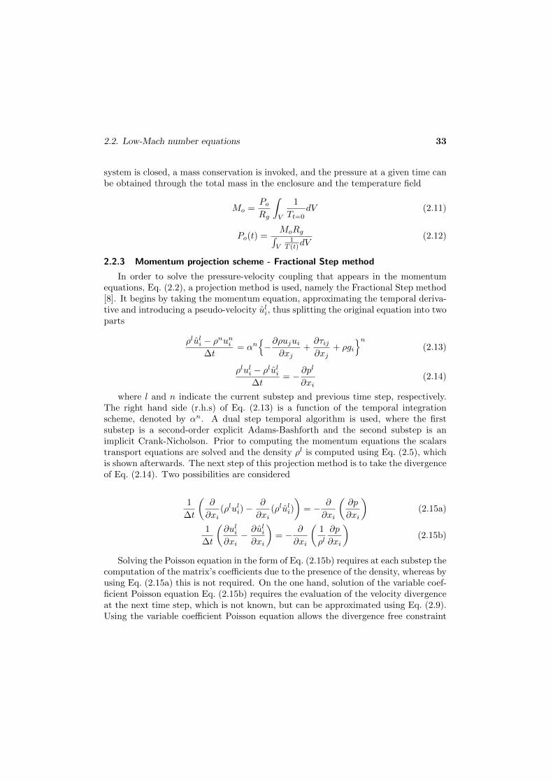
2.2. Low-Mach number equations 33
system is closed, a mass conservation is invoked, and the pressure at a given time canbe obtained through the total mass in the enclosure and the temperature field
Mo =PoRg
∫V
1
Tt=0dV (2.11)
Po(t) =MoRg∫V
1T (t)dV
(2.12)
2.2.3 Momentum projection scheme - Fractional Step method
In order to solve the pressure-velocity coupling that appears in the momentumequations, Eq. (2.2), a projection method is used, namely the Fractional Step method[8]. It begins by taking the momentum equation, approximating the temporal deriva-tive and introducing a pseudo-velocity uli, thus splitting the original equation into twoparts
ρluli − ρnuni∆t
= αn−∂ρujui
∂xj+∂τij∂xj
+ ρgi
n(2.13)
ρluli − ρluli∆t
= − ∂pl
∂xi(2.14)
where l and n indicate the current substep and previous time step, respectively.The right hand side (r.h.s) of Eq. (2.13) is a function of the temporal integrationscheme, denoted by αn. A dual step temporal algorithm is used, where the firstsubstep is a second-order explicit Adams-Bashforth and the second substep is animplicit Crank-Nicholson. Prior to computing the momentum equations the scalarstransport equations are solved and the density ρl is computed using Eq. (2.5), whichis shown afterwards. The next step of this projection method is to take the divergenceof Eq. (2.14). Two possibilities are considered
1
∆t
(∂
∂xi(ρluli)−
∂
∂xi(ρluli)
)= − ∂
∂xi
(∂p
∂xi
)(2.15a)
1
∆t
(∂uli∂xi− ∂uli∂xi
)= − ∂
∂xi
(1
ρl∂p
∂xi
)(2.15b)
Solving the Poisson equation in the form of Eq. (2.15b) requires at each substep thecomputation of the matrix’s coefficients due to the presence of the density, whereas byusing Eq. (2.15a) this is not required. On the one hand, solution of the variable coef-ficient Poisson equation Eq. (2.15b) requires the evaluation of the velocity divergenceat the next time step, which is not known, but can be approximated using Eq. (2.9).Using the variable coefficient Poisson equation allows the divergence free constraint

34Chapter 2. Numerical assessment of conservative unstructured discretisations for
Low-Mach flows
to be recovered in the limit of inviscid flows. On the other hand, when the constantcoefficient Poisson equation is considered, the mass divergence at the next time stepis an unknown, but it can be approximated using mass conservation Eq. (2.1). Thetemporal derivative of the density is then introduced into Eq. (2.15a). Even thoughthe advantages of the second formulation, Eq. (2.15b), the first one is preferred inthis work because of its lower computational effort at each substep. In both predictorand corrector substeps the pressure Poisson equation is solved using a Direct SchurDecomposition [25, 26].
Use of a constant coefficient Poisson equation requires the computation of themass divergence at the next substep ∇ · (ρu)l, which is not known. The continuityequation is then used to approximate it. This term has been reported to introducenumerical instabilities [9–11] and no closed form to approximate this time derivativehas been reported to be best suited.
In this work, the second-order backward approximation to the first derivative atthe l substep proposed by Nicoud [9] is used
∂ρ
∂t
∣∣∣∣l =
((∆tn + ∆tn−1)2 − (∆tn)2
)ρl − (∆tn + ∆tn−1)2ρn + (∆tn)2ρn−1
∆tn ∆tn−1 (∆tn + ∆tn−1)(2.16)
By using the continuity equation to approximate the mass divergence ∇ · (ρu)l,mass conservation is enforced. The gas state law Eq. (2.5) is used in its form at eachsubstep to compute the density. However, energy conservation is not satisfied as itcan be seen by the use of the non-conservative form of the energy equation, Eq. (2.3).As reported by Knikker [10], both constraints can only be met when an iterative timescheme is used, at the cost of a higher computational effort per iteration.
2.3 Unstructured discretisation
The discrete set of equations is obtained employing the finite-volume technique,where the governing equations Eq. (2.1)-(2.3) and Eq. (2.6) in differential form areintegrated giving a set of conservation equations to be solved at each control volume(CV).
The generic transport equation in integral form after applying Gauss theorem is∫V
∂ρφ
∂tdV = −
∫A
ρujnjφdA+
∫A
Γ∂φ
∂xj
∣∣∣∣∣f
njdA+
∫V
SdV
= −Cc +Dc + S · V
(2.17)
where φ represents any dependent variable (ui, Yk, T ) and C,D, S represent the con-vective, diffusive and extra terms, respectively. Approximating the surface integrals
2.3. Unstructured discretisation 35
as summation over cell faces, the discrete cell centred convective and diffusive termsbecome
Cc =∑f
φfρfui,fni,fAf (2.18a)
Dc =∑f
Γf (φnbcv − φcv)Afδf
(2.18b)
where φf represents an interpolation of φ at a cell face. In the diffusive term, thederivative of the variable at the face has been estimated using a centred approximationto the first derivative. The details of these interpolations will be discussed later. Thedistance δf for unstructured meshes is the distance between two nodes projected inthe normal direction to the face, δf = (si,fni,f ), where si,f is the vector from thecentroid of the control volume to the centroid of the neighbour control volume, as itcan be seen in Fig. 2.1.
Figure 2.1: Geometrical parameters used to define both collocated and staggeredformulations. Points P and F represent the cell centroids for collocated schemesand the cell circumcentres for staggered schemes.
Having defined the discrete form of the transport equations, in the following focusis placed on the spatial discretisation of the momentum equations in order to tacklethe pressure-velocity coupling. Two formulations for unstructured meshes are heredescribed, namely the collocated formulation detailed by Trias et al. [19] and Jofreet al. [20] and the staggered one of Perot [16].
The main difference between collocated and staggered formulations is the locationof the primary solution variables. Both collocated and staggered schemes place scalar

36Chapter 2. Numerical assessment of conservative unstructured discretisations for
Low-Mach flows
variables (ρ, p, h, T, Yk) at cell centres and the mass flow is placed at the cell faces.The velocity ui is stored at the cell centres in the collocated scheme and the massflux, ρu, at the face centres in the staggered scheme.
Collocated formulations are known to suffer from an odd-even decoupling of thepressure field due to pressure and velocity being placed at the same points, as shownby Patankar [27]. Additionally, it has also been shown that collocated formulationsdo not fully preserve kinetic energy. Morinishi et al. [28] showed that the error wasof O(∆tα∆x2
i ), with α depending on the temporal integration scheme. However,when dealing with complex geometries or when non-cartesian grids are considered,the collocated mesh scheme is usually preferred due to its simplicity, as opposedto staggered formulations, which require defining displaced meshes. Constructionof these displaced meshes is trivially performed for cartesian grids, but it is a morecomplex task for non-cartesian ones. Nonetheless, the method described by Perot [16]allows these displaced meshes to be built almost effortlessly. Staggered formulationspresent the advantage of not suffering from the pressure odd-even decoupling.
2.3.1 Collocated discretisation:
As described by Felten and Lund [15], collocated formulations suffer from twotypes of error. The first type is related to mass conservation, which also influenceskinetic energy conservation. The rationale is that the pressure field obtained from thePoisson equation Eq. (2.15), ensures mass conserving fluxes at the faces, but not forthe primary solution variables, which are located at the cell centres. This results ina pressure-velocity decoupling. In order to avoid it, a pressure correction to the cellcentred velocities is applied. Therefore, once the pressure equation Eq. (2.15) has beensolved, the cell centred velocities must be corrected using Eq. (2.14). Specifically, ifthe Poisson equation with constant coefficients is considered1, the cell centred velocitycorrection takes the form
uli,c = uli,c −∆t
ρlc
∂p
∂xi
∣∣∣∣lc
(2.19)
where the cell centred pressure gradient is evaluated using the Gauss theorem.The second type of error is related to the reconstruction of the mass flow at the
1An equivalent procedure is obtained in case the Poisson equation with variable coefficients isconsidered.

2.3. Unstructured discretisation 37
cells’ faces. On the predictor stage of the Fractional Step method2, once the pseudo-velocities uli have been computed using Eq. (2.13), the pseudo-mass flow has to beevaluated
ml= (ρui)
lfnifAf (2.20)
where (ρui)lf must be approximated. As shown by Felten and Lund [15], the
reconstruction of the variables at the faces is a critical issue. Therefore, in order tominimise errors in the conservation of the kinetic energy, the interpolation at the facesis performed by taking the average between neighbouring cells
ρui|lf =1
2(ρui|lcv + ρui|lnbcv) (2.21)
Once the velocity at cell centres is known, the mass flow at the cell faces’ isreconstructed accordingly
ml = (ρui)lfnifAf −∆t
∂p
∂xi
∣∣∣∣lf
(2.22)
where the face pressure gradient is approximated by a centred finite difference∂p∂xi|lf=
(plnbcv−plcv)
δfAf and the pseudo-velocity at the cell faces is obtained through
Eq. (2.19) and (2.21)
ρui|lf =1
2
((ρui|lcv + ∆t
∂p
∂xi
∣∣∣∣lcv
)+
(ρui|lnbcv + ∆t
∂p
∂xi
∣∣∣∣lnbcv
))(2.23)
The above equation is derived imposing mass conservation to the velocity fieldat the faces. As shown by Jofre et al.[20], by taking the divergence of Eq. (2.14),approximating the volume integrals by summation over the faces and requiring massconservation at an infinitesimal control volume at each face, Eq. (2.23) is obtained.The correction here presented reminds to the one presented by Rhie and Chow [29]based on a momentum-weighted interpolation strategy. Regarding the order of theerror in kinetic energy conservation, this scheme gives an error of O(∆t2∆xmi ), wherem = min(2, r) and r is the order of the interpolation of the velocities to the face.
2.3.2 Staggered discretisation:
As stated previously, staggered formulations place velocity and pressure at differ-ent grid locations. This methodology presents the advantage that inherently conservesmomentum, kinetic energy and circulation. Additionally, it does not present the odd-even decoupling found in collocated schemes. Thus, provided that the discrete oper-ators are conservative, this staggered scheme is fully conservative. These advantages
2Not to be confused with the predictor substep of the predictor-corrector time integration scheme.

38Chapter 2. Numerical assessment of conservative unstructured discretisations for
Low-Mach flows
come at the cost of requiring the construction of displaced meshes, which in struc-tured meshes are easily built but on unstructured meshes it is not a straightforwardtask.
The method here employed follows the formulation by Perot [16], who proposesa technique to construct a displaced control volume at each face and shows that theoverlapping of control volumes does not represent an issue. The construction of thestaggered cells is sketched in Fig. 2.1. The width of the displaced control volume isdefined as Wf = W cv
f +Wnbcvf where Wm
f is the distance from the face circumcentreto the “m” neighbour cell circumcentre (remember that nodes are located at the cellcentroid). The volume of the displaced control volume is then Vf = WfAf . Subindexs“cv” and “nbcv”, which refer to cells sharing the same face, are here maintained forconsistency with the collocated formulation. The described method assumes thatcells have a circumcentre, which is not required to be within a cell. However, highlydistorted grids can impact the accuracy of the method.
The staggered formulation uses the displaced mesh to integrate the face normalmass fluxes, ρu. Therefore, integrating3 Eq. (2.13), taken in the form of Eq. (2.17),over each displaced cell and taking the dot product with the face normal vector, thestaggered form of the fractional step is obtained, where the primary solution variableis the face normal mass flux
(ρu)lf − (ρu)nf∆t
Vf = αn−Ci,fni,f +Di,fni,f + ρfgini,fn (2.24)
where convective and diffusive terms have to be calculated at the faces. Notice thatthe integrated variable is an scalar value located at the face and in the face normaldirection. In the present formulation, convective and diffusive terms are interpolatedto the faces from the cell centred values using a weighted sum
Ci,f = W cvf
Ci,cvVcv
+Wnbcvf
Ci,nbcvVnbcv
(2.25a)
Di,f = W cvf
Di,cv
Vcv+Wnbcv
f
Di,nbcv
Vnbcv(2.25b)
where Ci,cv and Di,cv are calculated using Eq. (2.18). Analogously, for the pressurecorrection equation Eq. (2.14)
(ρu)|lf = (ρu)|lf −∆t(plnbcv − plcv)AfVf
(2.26)
3The derivation here presented deals with the momentum projection scheme with a constantcoefficient Poisson equation. Extension to the non-constant coefficient Poisson equation is straight-forward.

2.3. Unstructured discretisation 39
where, due to the method of construction of the displaced cells around the cells’ faces,the pressure gradient is computed as the pressure difference between the displacedcontrol volume faces. Thereafter, the procedure is akin to the one presented for thecollocated scheme. Taking the divergence of Eq. (2.26), a Poisson equation, Eq. (2.34),is obtained, where again the mass divergence at the next step is approximated throughthe continuity equation by the temporal derivative of the density Eq. (2.16). Once ithas been solved, the face mass fluxes are corrected by means of Eq. (2.26) withoutany further modifications.
Lastly, one critical aspect remains to be considered for Perot’s staggered formu-lation. The convective and diffusive operators have been approximated at the cellfaces using their corresponding values at the cell centres. However, in order to com-pute these values at the cell centres, the velocity field at those locations must becomputed. In this regard, two approaches are used in this work, the first order recon-struction (STAGG1) proposed by Perot [16], and a polynomial reconstruction method(STAGG2) proposed by Jofre et al.[20].
The first order reconstruction is based on Gauss’ divergence theorem applied tothe product of the mass flux ρui,c and the position ri at each cell∫
Vc
ρcui,c|ldV +
∫Vc
ri∂ρcuj,c|l
∂xjdV =
∑f
∫Af
(rj(ρuj |l)
)· nidA (2.27)
where ri = xi − x0,i represents the position with respect to the cell circumcentre.Then, assuming a constant mass field within the cell, thus making a first order ap-proximation within the cell and rendering the second term on the left hand side equalto zero, the cell centred velocity is computed through
uli,c =1
ρlcVc
∑f
ρfuli,fr
ci,fAf (2.28)
where rci,f = xfgi,f−xcci,c is the vector from the cell circumcentre xcci,f to the face centroid
xfgi,f .The second reconstruction method (STAGG2) uses a least square procedure to
obtain the cell centred velocities from the faces’ mass fluxes. To that end, the cellcentred velocity is approximated by a polynomial function around the cell centroid(uc(r) = a + bx + cy + dz) with the restriction that at the cell faces the computedmass fluxes have to be recovered
ρcui,c(r) ni,f = (ρui)|f (2.29)
Hence a linear system of equations is obtained where the coefficients (a,b, c,d) of thepolynomial are the unknowns. The resulting system is overdetermined, due to the

40Chapter 2. Numerical assessment of conservative unstructured discretisations for
Low-Mach flows
higher number of faces than unknowns. Therefore a least-squares method is used tosolve the system. As it can readily be seen, this second approach is computationallymore expensive than the STAGG1 method, mainly due to the need of solving a systemof equations for each cell.
2.3.3 Face interpolation schemes
As previously stated, when the convective and diffusive operators were discretised,there remained to be detailed the interpolations of the face centred values for theconvective term and the derivative at the faces for the diffusive term.
As shown by Verstappen and Veldman [18], in order to ensure good stabilityproperties of the numerical algorithm, even at high Reynolds numbers with coarsemeshes, it is necessary to preserve the properties of the differential operators in theirdiscrete counterparts. Therefore, the discrete convective operator is required to beskew symmetric, the negative conjugate transpose of the discrete gradient operatorto be exactly equal to the mass divergence operator and the diffusive terms to bestrictly dissipative, being the diffusive operator symmetric and positive definite. Theserequirements are mainly placed for the momentum equations, from which kineticenergy conservation is derived. Therefore, in the momentum equations cell face valuesrequired by the convective operator are interpolated using a second order SymmetryPreserving (SP) interpolation, which produces a skew symmetric discretisation
φf =1
2(φcv + φnbcv) (2.30)
Regarding the diffusive operator, as it has already been shown in Eq. (2.18), it isdiscretised by means of a two point centred approximation to the first derivative(CDS), thus obtaining a symmetric and positive definite matrix.
Concerning the transport equations for scalars, such as enthalpy, temperature ormass fractions, the above requirements of kinetic energy preservation do not apply.However the guidelines just presented for the construction of the discrete counterpartsof the differential operators are also applicable. Therefore, the discrete diffusive oper-ator is approximated in the scalars’ transport equations by means of the just detailedCDS scheme. With regard to the discretisation of the convective operator, additionalconsiderations have to be taken into account. When the local Peclet is high, centredapproximations to the derivatives were found to introduce oscillatory modes in theproblem resolution [27]. Therefore, upwinding-like interpolations were proposed toaddress this stability issue. The classical Upwind Difference Scheme (UDS), wherethe face value is approximated by the upwinding cell value, is known to be dissipa-tive and to introduce “false diffusion” effects, which are not desired in the currentframework. Higher order upwinding interpolations such as the Quadratic UpstreamInterpolation for Convective Kinematics (QUICK) [30] are able to deal with “falsediffusion” effects, while reducing their dissipative effect. As opposed to cartesian

2.3. Unstructured discretisation 41
meshes, where the upwind and downwind nodes can readily be selected, when dealingwith unstructured meshes several options are feasible as described by Segarra et al.[17]. In this work an extension to criterion C4 is used.
Criterion C4 generated new points on the face normal direction using only thenodal values and the gradient of the control volumes to which the face belonged,denoted in Fig. 2.2a as points C and D. In this work, instead of generating twopoints from the same nodal point, each point is the projection of a neighbouringcontrol volume node on the face normal direction, as shown in Fig. 2.2b. Then, theprojected variables’ values are obtained using their nodal value and the gradient attheir control volume. The advantage of the present method is that in case of using acartesian mesh, since the nodal points would already be on the face normal direction,the projected points would be the control volume nodes, thus recovering the originalQUICK scheme. On the other hand, using Criterion C4 two new points would stillbe generated from the same source point, therefore the final approximation would beof lower order.
(a) Criterion C4 from Segarra et al.[17]
(b) Present work.
Figure 2.2: Points for the QUICK scheme interpolations.
Having defined the upwind and downwind nodes, face values using the QUICKscheme [30], with Fig. 2.2b notation and considering non-equidistant placement of theprojected nodes, are computed
x =x− xU ′xD′ − xU ′
(2.31a)
φ =φ− φU ′φD′ − φU ′
(2.31b)

42Chapter 2. Numerical assessment of conservative unstructured discretisations for
Low-Mach flows
φf = xf +xf (xf − 1)
xC′(xC′ − 1)(φC′ − xC′) (2.31c)
where the overbar denotes non-dimensional values and values in the normal facedirection are obtained using the cell centred gradient
φC′ = φC +∇φ|C ·CC’ φD′ = φD +∇φ|D ·DD’ φU ′ = φU +∇φ|U ·UU’
For the QUICK scheme on unstructured meshes, this first interpolation or projec-tion diminishes its accuracy, and consequently its theoretical higher order propertiescan be lost. This aspect is discussed in Section 2.5.1. Nonetheless, false diffusioneffects are greatly diminished.
With the statements developed so far, coupled with the requirement in turbulentflows to use conservative schemes, in order to preserve kinetic energy, and as describedby Trias et al. [19] and Jofre et al. [20], showing the need for the convective operatorto be skew-symmetric and the diffusive operator to be symmetric and positive-definite,the Symmetry Preserving is used in the momentum equations. In the scalar transportequations both centred (SP, CDS) and upwinding schemes (UDS, QUICK) are used.In cases where the Peclet number is high, upwinding schemes are used, where theQUICK has been favoured over the UDS scheme due to its higher order properties.
2.3.4 Boundaries
Regarding values at boundaries of the computational domain, both collocated andstaggered formulations deal with them similarly. Dirichlet type conditions are imposedat face nodes. Neumann type conditions are applied analogously to the diffusive flux.Therefore, the flux at the face is computed using a one legged two point approximationto the first derivative. Concerning the displaced meshes in the staggered formulation,no displaced control volumes are created on the boundary faces. Similarly, in theevaluation of the convective operator, since values at the boundary faces are known,no interpolations such as Eq. (2.30) are needed.
2.4 Temporal Integration Algorithm
A variant of the predictor-corrector scheme shown by Najm et al.[7] is proposedhere to solve the set of equations Eq. (2.1)-(2.3) and Eq. (2.5). When chemicallyreacting flows are considered, Eq. (2.6) is also taken into account. The pressure-velocity coupling is solved using a fractional step projection method as described byNicoud [9], in which a constant coefficient Poisson results. This fractional stepping isdiscretised using both collocated [15] and staggered [16] formulations. In the predictorstep, a second-order Adams-Bashforth time integration scheme is used to calculatethe intermediate scalar and velocity fields. A pressure correction step ensures that thecontinuity equation, Eq. (2.1), is satisfied. The corrector step uses a Crank-Nicolson

2.4. Temporal Integration Algorithm 43
time integration scheme to advance the scalar fields. The velocity is reintegrated usingagain an Adams-Bashforth scheme, with the density at the next time step (n + 1).This corrector step also involves the resolution of a Poisson equation.
In explicit temporal algorithms, as shown by Knikker [10], the scalar transportequations must be expressed in non-conservative form because the density is com-puted afterwards, being itself a function of the previously computed scalars. Unlessan implicit approach is taken, both energy conservation Eq. (2.3) and gas state-lawEq. (2.5) cannot be simultaneously satisfied.
2.4.1 Temporal integration algorithm
In this subsection the explicit two-step temporal integration algorithm is described.Predictor-corrector schemes were proposed for low-Mach number flows due to thenumerical instabilities observed when a fully one step explicit time integration schemewas used [7].
Predictor1. Scalars are advanced using an Adams-Bashforth scheme
ρnφl − φn
∆t=
3
2
(ρn∂φ
∂t
∣∣∣∣n)− 1
2
(ρn−1 ∂φ
∂t
∣∣∣∣n−1)
(2.32)
where φ = Yk for the species equation and φ = h for the energy equation. InEq. (2.32), the first and second terms on the r.h.s are evaluated using Eq. (2.6)for the species and Eq. (2.3) for the energy transport, at time steps n and n−1.In these scalar transport equations no distinction is made between collocatedand staggered schemes as in both formulations scalar variables are stored at cellcentres.
2. Evaluate the thermodynamic pressure Po from Eq. (2.12), if it is not constant.
3. Evaluate the density ρl from the state equation Eq. (2.5), using the predictortemperature T l.
4. Pressure corrector step.
(a) Calculate the pseudo velocities using Eq. (2.13)
ρluli − ρnuni∆t
=3
2
(∂ρui∂t
∣∣∣∣n) − 1
2
(∂ρui∂t
∣∣∣∣n−1)
(2.33)
When using the collocated formulation, the temporal derivatives of thecell centred velocity in the above equation are computed using the discrete

44Chapter 2. Numerical assessment of conservative unstructured discretisations for
Low-Mach flows
version of Eq. (2.13) as detailed in Eq. (2.17). When dealing with thestaggered formulation, mass fluxes at the cell faces are integrated in timeand computed through Eq. (2.24).
(b) Solve the Poisson equation.
∂
∂xi
(∂pl
∂xi
)=
1
∆t
[∂
∂xi(ρluli)−
∂
∂xi(ρluli)
](2.34)
where the pseudo-mass flow, first term on the r.h.s, is obtained fromEq. (2.20) in the collocated scheme. This pseudo-mass flow is directlyobtained from the time integration, Eq. (2.24) and (2.33) in staggeredmeshes. The mass divergence at the next substep is approximated usingthe continuity equation Eq. (2.1)
∂
∂xi(ρluli) = −∂ρ
∂t
∣∣∣∣l(c) Calculate the predictor velocities
ρluli − ρluli∆t
= − ∂pl
∂xi(2.35)
This correction is applied to cell centred velocities in collocated schemes,while it is applied to face centred mass fluxes in staggered schemes.
(d) Final computations have to be performed for both formulations, as de-scribed in the previous section. In short, in the collocated scheme thefaces mass flow have to be computed using Eq. (2.22). Analogously, in thestaggered scheme the cell centred velocities have to be reconstructed fromthe face centred ones using either STAGG1 or STAGG2 reconstructionmethod.
CorrectorFor the sake of brevity, comments regarding staggered and collocated differences
have been omitted in this subsection. The reader is referred to the Predictor subsec-tion for differences between both spatial formulations within the temporal algorithm.
1. With the values computed at the Predictor step, the r.h.s. of Eq. (2.3) is usedto evaluate the time derivative of the predictor enthalpy (ρl−1 ∂h
∂t |l−1) and the
r.h.s. of Eq. (2.6) to evaluate the time derivative of the predictor mass fraction(ρl−1 ∂Yk
∂t |l−1). Then, the time derivative at the next time is evaluated using a
Crank-Nicholson scheme

2.5. Numerical Tests 45
ρl−1φn+1 − φn
∆t=
1
2
(ρn∂φ
∂t
∣∣∣∣n + ρl−1 ∂φ
∂t
∣∣∣∣l−1)
(2.36)
where φ = Yk for the species equation and φ = h for the energy equation.
2. Evaluate the thermodynamic pressure Po from Eq. (2.12), if it is not constant.
3. Using the ideal gas law Eq. (2.5), the density field at the next time step iscomputed.
4. Finally, the pressure corrector step to compute the velocity field.
(a) Calculate the pseudo velocities using Eq. (2.13)
ρn+1uli − ρnuni∆t
= r.h.s. Eq. (2.33) (2.37)
(b) Solve the Poisson equation.
∂
∂xi
(∂pn+1
∂xi
)=
1
∆t
[∂
∂xi(ρn+1uli)−
∂
∂xi(ρn+1un+1
i )
](2.38)
where, as in the predictor stage the momentum divergence ∇ · (ρn+1un+1)is replaced, using the continuity equation Eq. (2.1), by the density timederivative Eq. (2.16).
(c) Calculate the velocities at the next time step
ρn+1un+1i − ρn+1uli
∆t= −∂p
n+1
∂xi(2.39)
(d) In collocated schemes, the face mass flow mn+1f has to be computed using
Eq. (2.22). Analogously, in staggered schemes the cell centred velocitiesun+1i,c have to be reconstructed from the face centred mass fluxes using
using either STAGG1 or STAGG2 reconstruction method.
2.5 Numerical Tests
In the following the numerical schemes presented are tested in order to studythe effect of non-structured meshes. The general purpose unstructured and parallelobject-oriented CFD code TermoFluids [31] is used in this work. Three test cases arediscussed. Test Case 1 consists in a numerical reconstruction of a solenoidal field,

46Chapter 2. Numerical assessment of conservative unstructured discretisations for
Low-Mach flows
which is used to assess the accuracy of the interpolation schemes. Test Case 2 is adifferentially heated cavity under a large temperature difference, through which thespatial discretisation of the low Mach equations is analysed. Test Case 3 is a self-igniting turbulent jet flame, whereby the effect of the spatial discretisations on thetransient algorithm is evaluated.
2.5.1 Test Case 1 - Interpolation schemes accuracy
The accuracy of the presented interpolation schemes is studied by means of anexact sinusoidal function, Test Case 1. The reduction of the interpolations numericalerror with respect to the exact analytical value provides the order of accuracy. Thetarget function to be interpolated is a sinusoidal function
ψ =1
2πLsin(2πLx)cos(2πLy) (2.40)
This function is used twofold, as the function to be interpolated at the faces andas a stream function from which the velocity field is derived by taking the rotationalof the function ~u = ∇ x ψ
ux = −sin(2πLx)sin(2πLy)
uy = −cos(2πLx)cos(2πLy)
uz = 0
(2.41)
This velocity field is used by the upwinding schemes to determine the upwind anddownwind nodes. The numerical domain is a cube of length unit (L=1) in each di-mension. To carry out the grid refinement study, instead of creating several meshes,the length scale, or wavelength, of the sinusoidal function is modified. With thisstrategy, a single mesh of nCV volumes is generated and then the mesh is coarsenedby increasing the length scales of the function with respect to the mesh average spac-ing. Therefore, in order to quantify the amount of scales actually being capturedby the mesh two quantities have to be defined. In the first place, the average meshspacing is defined as Vavg = 1
nCV
∑c Vc, which allows defining an average mesh spac-
ing as ∆xavg = 3√Vavg. Secondly, the effective length of the domain is defined as
Leff = 1/L, where L is an integer value, which controls the sinusoidal wavelength.In consequence, the relative mesh size is ∆xavg/Leff = ∆xavgL.
In order to assess the influence of the unstructured meshing on the face interpo-lations, two meshes were generated: a structured one and an unstructured one. Bothmeshes have similar average mesh spacings and the relative mesh spacings rangedfrom 0 to 0.4. For each relative mesh size the values of the function Eq. (2.40) wereinterpolated at the faces using the analytical values at the cell centres. The error ε is

2.5. Numerical Tests 47
then computed as the root mean square (rms) between the numerical approximationsand the analytical values computed at the faces
ε =
√1
nF
∑f
ε2f (2.42)
where εf is the error in each face value and nF is the number of faces. The errorsof the interpolations along with their accuracy are plotted in Fig. 2.3. Four interpo-lation methods are here presented: the Symmetry Preserving (SP) scheme, which isequivalent to an average, the UDS, the QUICK and, for completion, a Central Differ-ence Scheme using Criterion I1a of Segarra et al.[17] (CDS2), which makes a linearinterpolation between neighbouring nodes and takes into account non-equal distancesbetween the face and the neighbouring nodes.
0
0.05
0.1
0.15
0.2
0.25
0.3
0.35
0.4
0 0.05 0.1 0.15 0.2 0.25 0.3 0.35 0.4
Normalized error
Relative mesh size
unstr SP
unstr QUICK
unstr UDS
unstr CDS2
a=0.47,m=1.31, unstr SP
a=1.32,m=1.78, unstr QUICK
a=0.73,m=0.98, unstr UDS
struct SP
struct QUICK
struct UDS
struct CDS2
a=0.84,m=1.91, struct SP
a=1.84,m=2.31, struct QUICK
a=0.84,m=0.97, struct UDS
Figure 2.3: Test Case 1 - Accuracy of the numerical interpolations in structured(‘struct’) and unstructured (‘unstr’) meshes. Dots represent the computed errorsand lines show the accuracy of each interpolation in the form ε = ahm, where hdenotes the mesh spacing and m indicates the order of accuracy.

48Chapter 2. Numerical assessment of conservative unstructured discretisations for
Low-Mach flows
A first aspect to be highlighted is that the order of accuracy of the differentmethods is the expected on structured meshes. On unstructured meshes, the orderdecreases for both the SP and the QUICK schemes. The UDS’ order of accuracyremains almost unchanged. However, the cause for the deterioration is different foreach scheme. On the one hand, in the QUICK scheme, as described previously, thegradients of the cell values are used to approximate the value on the normal directionto the face. This intermediate interpolation is a first order approximation, which isresponsible for the reduction of the interpolation order. On the other hand, centraldifference schemes, both SP and CDS2, mainly deteriorate due to non-orthogonaleffects. Additionally, comparing the SP with the CDS2 scheme, both schemes behavealmost identically on both structured and unstructured meshes, indicating that thenon-equal weights in the CDS are of minor importance in contrast to non-orthogonaleffects.
It should be noted that the UDS scheme on unstructured meshes presents lowererrors than on structured meshes. This may be attributable to the likely alignmentof the unstructured mesh with the solution. Nonetheless, in both cases the accuracyof the scheme is first order as expected.
Considering these results, it can be seen that the slight errors introduced using SPdiscretisations in the momentum equations, compared to CDS scheme, are compen-sated by the reported gain in numerical stability [15, 18] when using kinetic energypreserving formulations in turbulent flows. From these results, it can also be inferredthat low order approximations present in the construction of high order schemeson unstructured meshes causes a deterioration of the properties of those high orderschemes. Nonetheless, the accuracy order of the QUICK schemes is higher than theUDS and even SP scheme.
Finally, it should be noted that though the QUICK scheme presents a higher orderof accuracy, on coarse meshes, the SP produces a lower level of error. Nonetheless,as the mesh is refined the errors of the QUICK scheme become lower and at a fasterrate than the SP. Therefore, in scalar transport equations the QUICK scheme is agood alternative in cases where due to stability issues, centred approximations arenot viable.
2.5.2 Test Case 2 - Analysis of the spatial discretisations
The differentially heated square cavity, Test Case 2, benchmark case [21, 32] ofside L=1 under a large temperature difference (∆T = 720K) is used. The cavityleft wall is at a high temperature (Th) and the right wall is at a low temperature(Tc). These temperatures are related to the temperature difference by ε = Th−Tc
2T0.
Here a value of ε = 0.6 has been taken, in order to match the benchmark case. Thetemperature ratio defined between the highest temperature Th and the lowest Tc is4. As reported by Najm [7], for ratios higher than 2 at least a predictor-correctorscheme, as the one here proposed, is necessary.

2.5. Numerical Tests 49
The top and bottom walls are considered adiabatic. The fluid filling the cavity is airwith a constant Prandtl number (Pr = 0.71) and a constant specific heat capacity(cp = γRg/(γ−1) where Rg = 287 J/(kg K) and γ = 1.4). Its dynamic viscosity andthermal diffusivity follow Sutherland’s law
µ(T )
µref=
(T
Tref
)3/2Tref + 110.5
T + 110.5(2.43a)
κ(T ) =µ(T )cpPr
(2.43b)
where the reference temperature for this expression has been taken as Tref = 273Kand the reference viscosity is µref = 1.68·10−5kg/(m s). The ideal gas law Eq. (2.5) is
used to calculate the density. The Rayleigh number(Ra = Pr
gρ2o∆TL3
Toµ2o
)considered
here corresponds to the laminar regime (Ra = 106). With these parameters andthe reference conditions (Po0 = 101325Pa, T0 = 600K, and ρ0 = Po0/(RgT0)) theproblem is defined.
To study the accuracy of the described predictor-corrector scheme on unstructuredmeshes several uniform unstructured meshes were created, whose mesh spacings wereL/Np, where Np is the number of points at the boundaries. With this definition ofthe mesh spacing, equivalent structured uniform meshes are easily defined4. Uniformmeshes were chosen in order to minimise variations in mesh properties such as cells’aspect ratio, measuring the ratio between the smallest cell’s face area and its biggest,and orthogonality factor, measuring the angle between a face normal and the vectorjoining the neighbours cells centroids.
Fig. 2.4 shows the numerical errors of the thermodynamic pressure Po, where theerror is defined with respect to the reference case [32], shown in Table 2.1. It canbe seen that the convergence rate of the global algorithm is between first and secondorder.
The collocated scheme, using either SP or QUICK in the energy equation, and thestaggered scheme using STAGG2 reconstruction method with the QUICK show simi-lar results, being their convergence rate close to second order. The STAGG2 methodwith the SP shows first order accuracy, which indicates that interpolation errors inthe energy equation due to the SP affect the cell centred velocities reconstruction.The staggered scheme using the STAGG1 reconstruction method shows a lower con-vergence rate, which is of first order. This lower order of convergence for the STAGG1will be discussed in the following, along with convergence rate of the Nusselt numberat the wall. Comparing the curves for the SP and the QUICK schemes, it can be seen
4For example, if a uniform structured mesh were to be used to discretise the horizontal directionof the square cavity with Np = 64, the mesh spacing would be 1/64 = 0.0156

50Chapter 2. Numerical assessment of conservative unstructured discretisations for
Low-Mach flows
Discretisation Collocated Staggered (Stagg2) Ref. [32]Case Unstruct. Struct. Unstruct.
Scheme SP QUICK SP QUICK -Po/Po,0 0.9249 0.9237 0.9262 0.9250 0.9245Nuh 8.6864 8.7013 8.6742 8.6742 8.6866Nuc 8.6859 8.6461 8.6739 8.6358 8.6866
Nuh−Nuc0.5(Nuh+Nuc)
0.0058% 0.6358% 0.0030% 0.5948% 0%
Table 2.1: Results for the Differentially Heated Cavity with Ra = 106 using amesh spacing of 1/320.
that the errors on the coarse meshes are noticeably higher for the QUICK scheme.However, when finer meshes were used, the QUICK scheme delivered errors similar tothe SP scheme. As was mentioned in Sec. 2.3, momentum equations are solved usingSP, while different schemes are used for the scalar transport equations.
Fig. 2.5 shows the error for the Nusselt number at the hot wall with respect tothe reference case [32]. The evaluation of the heat fluxes is performed analogously tothe evaluation of the diffusive flux in the discrete transport equations, Eq. (2.18b).
As described for Fig. 2.4, similar trends are observed regarding the order of ac-curacy for both collocated and structured staggered schemes. The global behaviourof the algorithm is between first and second order, with the exception the staggeredscheme using STAGG1 reconstruction method
First-order accuracy for the local Nusselt number is expected due to the approxi-mation to the first derivative, where a two point one legged stencil is used. However,globally the Nusselt number is seen to behave between first and second order. Theinfluence of the different schemes, which were used for the convective term, is of minorimportance, causing small variations on the actual error.Considering the first-order accuracy for a local value, such as the Nusselt number atthe wall, and the almost second-order accuracy for a global value, such as the thermo-dynamic pressure and the average Nusselt number at the walls, serves to illustrate theincrease in accuracy from local approximations of the operators to the global scheme,due to error cancelling within the mesh [33].
Additionally, it must be highlighted that the results obtained with the staggeredformulation using the STAGG1 reconstruction method on unstructured meshes showan accuracy of order zero, regardless of the convective discretisation scheme. How-ever, if structured meshes are considered, the computed accuracy is between first andsecond order. The justification of this phenomenon may be attributed to the cellcentred velocities reconstruction. Comparing the results obtained with the STAGG1staggered formulation, unstructured against structured, it can be inferred that the or-

2.5. Numerical Tests 51
1e-05
0.0001
0.001
0.01
0.1
1
0.001 0.01
Error P0
Mesh spacing L/Np
Coll SPColl QUICKStagg1 SP
Stagg1 QUICKStagg2 SP
Stagg2 QUICK1st order2nd order
Figure 2.4: Test Case 2 - Numerical error for the thermodynamic pressure usingunstructured meshes. For comparison, short-dashed-dotted and long-dashed-dottedlines are plotted, showing first and second order convergence rates. Mesh spacingis expressed in terms of equivalent uniform structured mesh number of points, Np.
der of accuracy of the cell centred velocities reconstruction in the unstructured meshesbecomes null, whereas on the structured ones it is of first order. Thus, the errors inreconstructing the cell centred velocities affect the evaluation of the convective term,which in turn affect the magnitude of the diffusive term. Structured meshes do notsuffer from this deterioration of the solution due to their inherent geometric proper-ties. Still, it can be seen in Fig. 2.5 that results obtained using the STAGG1 methodconverge to a solution, indicating that the computed velocity fields on each meshare intrinsically coherent, although incorrect. Additional simulations were conductedwhere the second term on the right hand side of Eq. (2.27) was not assumed to be zero,to test the influence of this assumption. However, steady state results did not varybecause at the stationary state mass divergence is zero, since transient density varia-tions are null. Therefore, higher order approximations are required for the cell centred

52Chapter 2. Numerical assessment of conservative unstructured discretisations for
Low-Mach flows
1e-05
0.0001
0.001
0.01
0.1
1
0.001 0.01
Error Nuhw,avg
Mesh spacing L/Np
Coll SPColl QUICKStagg1 SP
Stagg1 QUICKStagg2 SP
Stagg2 QUICKStagg1 SP struct
1st order2nd order
Figure 2.5: Test Case 2 - Numerical error of the averaged Nusselt number atthe hot wall. For comparison, short-dashed-dotted and long-dashed-dotted linesare plotted, showing first and second order convergence rates, respectively. Meshspacing is expressed in terms of equivalent uniform structured mesh number ofpoints, Np.
velocities reconstruction, such as the STAGG2 reconstruction method, which is shownto provide accurate results. However, as previously stated, the STAGG2 method iscomputationally more demanding, which hinders its viability. Results for the finermesh are not reported for the STAGG2 method due to computational limitations.However it can be seen that the staggered method using the STAGG2 reconstructionshows a similar trend as the collocated method.
With respect to the cold wall, trends are similar as at the hot wall although minordiscrepancies are noticeable. The reason is that the boundary layer is thinner atthe cold wall than at the hot wall, therefore smaller grid spacings are required tocorrectly characterise the thermal boundary layer at the cold wall. However, in thiswork successive uniform meshes have been used.
Concerning the noticeable lower error for the mesh with equivalent spacing 1/320,it should be remarked that these small errors are caused by supraconvergence effects,which lower the errors globally, as described by Trias et al. [33]. It should be borne inmind that although uniformly spaced meshes were used, in unstructured meshes therecan be variations in the cells properties, such as aspect ratio, orthogonality, amongothers, which can cause deviations in the theoretical trends.
Due to the use of the non-conservative form of the energy equation, it was stated

2.5. Numerical Tests 53
that the algorithm would produce an error in the energy error. Its reduction asthe mesh is refined is shown in Fig. 2.6. On the one hand, it can be seen that theSymmetry-Preserving scheme is not capable of reducing this error. On the otherhand, the QUICK scheme is capable of reducing it. However, on coarser meshes, theSP scheme results in a lower error than the QUICK scheme, which is similar to thepreviously shown results.
0.0001
0.001
0.01
0.1
1
10
0.001 0.01
Mesh spacing L/Np
Energy equation error
Coll SPColl QUICKSTAGG1 SP
STAGG1 QUICK
STAGG2 SPSTAGG2 QUICK
1st order2nd order
Figure 2.6: Test Case 2 - Error in the energy equation. For comparison, short-dashed-dotted and long-dashed-dotted lines are plotted, showing first and secondorder convergence rates.
Finally, detailed results comparing the SP and QUICK schemes using a meshspacing of 1/320 are shown in Table 2.1 along with the reference results. For thestaggered formulation, only results using the STAGG2 reconstruction method arereported, because the computed values with STAGG1 reconstruction method werenot in accordance. It can be seen that the QUICK suffers a deterioration due to thelower order intermediate interpolations. Furthermore, the QUICK scheme deviatesfurther from the mean in the cold wall. This behaviour is attributable to the factthat the boundary layer is thinner in the cold wall.
2.5.3 Test Case 3 - Analysis of the transient behaviour
The experimental configuration by Markides and Mastorakos [23] is used to testthe transient behaviour of the proposed numerical algorithm. It consists of a fuel

54Chapter 2. Numerical assessment of conservative unstructured discretisations for
Low-Mach flows
jet with a preheated co-flowing air stream, as shown in Fig. 2.7. The co-flowing airis forced to pass through a perforated plate to promote turbulence. The perforatedplate (3.0mm holes and 44% blockage) is located 63mm upstream of the fuel nozzleto allow turbulence to develop. The fuel nozzle has a diameter of 2.25mm and is thinwalled (0.32mm). The main test section consists of a 500mm long and 25mm innerdiameter vacuum insulated quartz tube. The reference experiments were performedover a wide range of operating conditions and four regimes, namely ’No ignition’,’Random spots’, ’Flashback’, and ’Lifted flame’ were identified.
Figure 2.7: Autoignition experimental configuration (Test Case 3 ).
In the present work the ’Random spots’ regime is simulated, Test Case 3, whereautoignition kernels appear but are quenched and convected out of the domain beforethey can act as a flame anchoring point or cause flashback. The fuel is a mixture of H2
and N2 (YH2= 0.13, YN2
= 0.87) at 750K and the co-flow oxidizer is air (YO2= 0.233,
YN2= 0.767). For the ’Random spots’ regime, the oxidiser temperature is 950K.
Both fuel and air inlet velocities are 26m/s. The fuel jet Reynolds number is 330and the coflow Reynolds number is 5800. The simulation domain spanned from thefuel jet nozzle up to 135mm in the downstream direction. In order to reproduce theturbulence generated by the perforated plate, an auxiliary non-reactive simulation wasperformed in an annular mesh, recreating the physical domain upstream to the injectorlips. In this non-reacting simulation, the plate was placed inside the domain using theimmersed boundary technique. The solution of this non-reactive simulation was thenstored and afterwards loaded during the reactive CFD simulation. This method allowsa significant saving of computational resources during the numerical simulation, and

2.5. Numerical Tests 55
develops a realistic divergence-free velocity field, as opposed to synthetic turbulencegenerators based on digital filters. For the fuel jet, a laminar parabolic velocity profileis assumed.
Since the test case here considered is of turbulent nature, the set of transportequations Eq. (2.1)-(2.3), (2.5) and (2.6) previously presented have to be formulatedin the context of Large Eddy Simulations (LES) models using Favre-filtered quantitiesand closures for the subgrid turbulent fluxes have to be introduced. For the sake ofbrevity, the equations are not here rewritten, but it is just stated that the variablesare Favre-filtered quantities and that in the right hand side of the equations, thereappears an extra term representing the subgrid turbulent transport. Closure for themomentum turbulent stresses is preformed by means of the Wall-Adapting LocalEddy-viscosity (WALE) model [34]. The scalar subgrid turbulent fluxes are modelledusing a constant turbulent Schmidt number with value 0.4. The chemical sourceterm is treated explicitly, thus the filtered reaction terms are assumed to be equal tothe reaction rate computed using the filtered quantities ˜wk(Yk, T ) = wk(Yk, T ). Thedetailed chemical mechanism of Mueller et al. [35] is used, which involved 9 speciesand 21 reactions.
Numerical simulations were performed using a collocated discretisation on a 4 ·105
CV unstructured mesh. Mesh refinement was performed near the air-fuel shear layer.Since the temporal scheme is independent from the spatial discretisation, the presentcase is analysed using only the collocated formulation. The decision is justified by thebetter behaviour of the collocated scheme compared with the staggered scheme usingthe first order velocity reconstruction method (see Sec. 2.5.2). Additionally, as shownby Jofre et al. [20] in LES simulations of turbulent flows, the required meshes are fineenough to make the kinetic error of the collocated formulation imperceptible to thephysics of the problem. Furthermore, no significant differences are expected betweenstaggered formulation with the STAGG2 method and the collocated one, based onthe results of a turbulent flow by Jofre et al. [20]. Additionally, no mesh refinementwas performed since changes in the mesh would modify the effect of the LES model.
In the random spots case, the ignition length oscillates around a mean distancefrom the fuel inlet. This is caused by the appearance of random autoignition kernels,which are quenched and convected out of the domain. Several snapshots of the processare shown in Fig. 2.8, where it can be seen that the mixture ignites at different axiallocations.
Fig. 2.9 shows the evolution of autoignition lengths in time for the random spotsregime for different numerical schemes used in the scalar equations. The ignitionlength is determined using as criterion a rise of 1% in the initial co-flow tempera-ture [36]. Upwinding schemes, namely the UDS and QUICK schemes, show goodagreement with the experimental data. Furthermore, the QUICK is seen to repro-duce accurately the experimental data. Explicit treatment of chemical reactions is

56Chapter 2. Numerical assessment of conservative unstructured discretisations for
Low-Mach flows
Figure 2.8: Test Case 3 - Instantaneous snapshots of the temperature. Timescale is adjusted to the beginning of fuel injection (t = 0). The axial length of thecomputational domain is 135mm. Results computed using the UDS scheme.
shown to perform adequately for the current Reynolds numbers. Regarding the CDS2scheme, it features ignition spots at two different heights. One close to the fuel nozzleexit and another at a higher axial location, which is also shorter than the distancepredicted when using the UDS scheme. These upstream ignition kernels are a productof numerical diffusion caused by the numerical scheme and they do not achieve a tem-perature high enough to ignite a meaningful quantity of the mixture and stabilise theautoignition process at this short distance. The higher axial autoignition distancescaptured by the CDS2, which are similar to those of the upwinding schemes, showwhere the mixture is actually being completely burned. Comparing the QUICK andUDS schemes, the influence of the numerical diffusivity introduced by the UDS canbe seen by the shorter autoignition distances predicted by it.
2.6 Conclusions
In this chapter, both collocated and staggered spatial discretisations for unstruc-tured grids have been analysed in the context of low Mach flows. A new approach todefine the upwind and downwind nodes of the QUICK inteporlation scheme has been

2.6. Conclusions 57
0
10
20
30
40
50
60
70
0 2 4 6 8 10
CDS2 min
CDS2 mean
Exp. min
QUICK mean
Autoignition length [mm]
Time [ms]
Exp.UDS
CDS2QUICK
Exp. mean
UDS mean
UDS minQUICK min
Figure 2.9: Test case 3 - Autoignition distances for the random spots regime.Horizontal lines represent mean and minimum autoignition distances for each nu-merical scheme and the experimental data. For the latter only mean and minimumvalues are plotted.
presented. SP, UDS and QUICK discretisation schemes have been assessed in bothstructured and unstructured meshes. It has been shown that the QUICK schemedid not provide the expected order of accuracy on unstructured meshes due to inter-mediate interpolation errors. Therefore, concerning the interpolations in the scalar’sequations, low order schemes are best suited in coarse meshes. When finer meshesare used, it is worth switching to higher order schemes.
Regarding the spatial discretisations, collocated and staggered schemes have beendescribed to be used on unstructured meshes. Following Felten and Lund [15], inthe collocated scheme the cell faces mass fluxes are computed using an average, evenin unstructured grids. The aim is to minimise errors in the conservation of kineticenergy. Despite the use of constant coefficients for the computation of the cell facesmass fluxes, the numerical results showed good agreement with the reference data.Concerning the staggered discretisation, it has been shown that the cell centred veloc-ity reconstruction plays a central role in its correct behaviour. The original first-orderreconstruction method has been shown to perform correctly on structured meshes.However, when unstructured meshes were considered, a convergence of the resultscould be observed, albeit to a different solution than the reference one. The new

58 References
approach proposed by Jofre et al. [20], which has been extended to variable-densityflows, improved the behaviour of the scheme. However, the computational resourcesincreased considerably.
Both reacting and non-reacting test cases were carried out using a Symmetry-Preserving scheme for the cell face velocities interpolations. Overall, good agreementbetween the reference data and the presented results has been shown, despite usingconstant weights for the cell faces velocity interpolations, even in non-uniform grids.Nonetheless, the purpose of this schemes is to preserve kinetic energy.
A benchmark differentially heated cavity, Test Case 2, has been numerically stud-ied. In general, the numerical algorithm applied to solve this case showed almostsecond-order behaviour. However, as initially discussed, the algorithm presents an in-trinsic error in the energy conservation due to the temporal scheme. Since an explicittime integration is used, mass conservation and the ideal gas state law can be met atthe cost of using the energy equation in its non-conservative form.
In Test Case 3, the self-igniting turbulent case, it has been shown the effect ofnumerical diffusion on the auto-ignition location of a flame. The CDS2 scheme ex-hibited numerically caused ignition spots. Similarly, comparing the mean ignitiondistances between the UDS and QUICK schemes, the diffusive nature of the UDSscheme resulted in shorter distances than the QUICK. Nonetheless, good agreementusing both UDS and QUICK schemes was found with the experimental data.
References
[1] D.D. Gray and A. Giorgini. The validity of boussinesq approximation for liquidsand gases. International Journal Of Heat And Mass Transfer, 19:545–551, 1976.
[2] J. Vierendeels, J. Merci, and E. Dick. Numerical study of natural convective heattransfer with large temperature difference. International Journal of NumericalMethods for Heat and Fluid Flow, 11(4):329–341, 2001.
[3] T. Kloczko, C. Corre, and A. Beccantini. A matrix-free implicit method for flowsat all speeds. In Proc. ICCFD3 Conference, Toronto, Canada, 11–15 July, 2004.
[4] E. Becker and M. Braack. Solution of a stationary benchmark problem for naturalconvection with large temperature difference. International Journal Of ThermalSciences, 41:428–439, 2002.
[5] M. Darbandi and S.F. Hosseinizadeh. General pressure-correction strategy toinclude density variation in incompressible algorithms. Journal of Thermophysicsand Heat Transfer, 17(3):372–380, 2003.
[6] L. Shunn, F. Ham, and P. Moin. Verification of variable-density flow solvers usingmanufactured solutions. Journal of Computational Physics, 231:3801–3827, 2012.

References 59
[7] Habib N. Najm, Peter S. Wyckoff, and Omar M. Knio. A semi-implicit numericalscheme for reacting flow. Journal of Computational Physics, 143:381–402, 1998.
[8] J. Kim and P. Moin. Application of a fractional-step method to incompress-ible Navier–Stokes equations. Journal of Computational Physics, 59(2):308–323,1985.
[9] F. Nicoud. Conservative high-order finite difference schemes for low-mach numberflows. Journal of Computational Physics, 158:71–97, 2000.
[10] R. Knikker. A comparative study of high-order variable -property segregatedalgorithms for unsteady low mach number flows. International Journal for Nu-merical Methods in Fluids, 66:403–427, 2011.
[11] B. Lessani and M.V. Papalexandris. Time-accurate calculation of variable densityflows with strong temperature gradients and combustion. Journal of Computa-tional Physics, 212:218–246, 2006.
[12] M. Darbandi and S.F. Hosseinizadeh. Numerical simulation of thermobuoyantflow with large temperature variation. Journal of Thermophysics and Heat Trans-fer, 20(2):285–296, 2006.
[13] C.-D. Munz, S. Roller, R. Klein, and K.J. Geratz. The extension of incompressibleflow solvers to the weakly compressible regime. Computers and Fluids, 32:173–196, 2003.
[14] H. Reza Ebrahimi-Kebria1, M. Darbandi, and S.F. Hosseinizadeh. Numericalsimulation of low-mach-number laminar mixing and reacting flows using a dual-purpose pressure-based algorithm. Numerical Heat Transfer, Part B: Fundamen-tals, 59:495–514, 2011.
[15] F.N. Felten and T.S. Lund. Kinetic energy conservation issues associated with thecollocated mesh scheme for incompressible. Journal of Computational Physics,215:465–484, 2006.
[16] B. Perot. Conservation properties of unstructured staggered mesh schemes. Jour-nal of Computational Physics, 159:58–89, 2000.
[17] C.D. Perez-Segarra, C. Farre, J. Cadafalch, and A. Oliva. Analysis of different nu-merical schemes for the resolution of convection-diffusion equations using finite-volume methods on three-dimensional unstructured grids. Part I: discretizationschemes. Numerical Heat Transfer, Part B: Fundamentals, 49:4:351–375, 2006.
[18] R.W.C.P. Verstappen and A.E.P. Veldman. Symmetry-preserving discretizationof turbulent flow. Journal of Computational Physics, 187:343–368, 2003.

60 References
[19] F.X. Trias, O. Lehmkuhl, A. Oliva, C.D. Perez-Segarra, and R.W.C.P. Verstap-pen. Symmetry-preserving discretization of Navier-Stokes equations on collo-cated unstructured grids. Journal of Computational Physics, 258(1):246–267,2014.
[20] Ll. Jofre, O. Lehmkuhl, J. Ventosa, F. Xavier Trias, and A. Oliva. Conserva-tion properties of unstructured finite-volume mesh schemes for the Navier-Stokesequations. Numerical Heat Transfer, Part B: Fundamentals, 65(1):53–79, 2013.
[21] P. Le Quere, C. Weisman, H. Paillere, J. Vierendeels, E. Dick, E. Becker,M. Braack, and J. Locke. Modelling of natural convection flows with large tem-perature differences: a benchmark problem for low mach number solvers. part1. reference solutions. ESAIM: Mathematical Modelling and Numerical Analysis,39(3):609–616, 2005.
[22] J. Vierendeels, B. Merci, and E. Dick. Benchmark solutions for the naturalconvective heat transfer problem in a square cavity with large horizontal tem-perature differences. International Journal of Numerical Methods for Heat andFluid Flow, 13(8):1057–1078, 2003.
[23] C. Markides and E. Mastorakos. An experimental study of hydrogen autoignitionin a turbulent co-flow of heated air. Proceedings of the Combustion Institute,30:883–891, 2005.
[24] T. Poinsot and D. Veynante. Theoretical and Numerical Combustion. R.T.Edwards Inc., 2005.
[25] F.X. Trias, M. Soria, C.D. Perez Segarra, and A. Oliva. A direct schur-fourier decomposition for the efficient solution of high-order poisson equations onloosely coupled parallel computers. Numerical Linear Algebra with Applications,13(4):303–326, 2006.
[26] R. Borrell, O. Lehmkuhl, M. Soria, and A. Oliva. Schur complement methodsfor the solution of poisson equation with unstructured meshes. Proceedings ofthe Parallel CFD Conference, pages 1–8, 2007.
[27] S. V. Patankar. Numerical heat transfer and fluid flow. Hemisphere PublishingCorporation, 1980.
[28] Y. Morinishi and T.S. Lund. Fully conservative higher order finite differenceschemes for incompressible flow. Journal of Computational Physics, 143:90–124,1998.
[29] C.M. Rhie and W.L. Chow. A numerical study of the turbulent flow past anisolated airfoil with trailing edge separation. AIAA Journal, 21:1525, 1983.

References 61
[30] B.P. Leonard. A stable and accurate convective modelling procedure based onquadratic upstream interpolation. Computer Methods in Applied Mechanics andEngineering, 19:59–98, 1979.
[31] O. Lehmkuhl, C.D. Perez Segarra, R. Borrell, M. Soria, and A. Oliva. Ter-mofluids: A new parallel unstructured CFD code for the simulation of turbulentindustrial problems on low cost PC cluster. Proceedings of the Parallel CFDConference, pages 1–8, 2007.
[32] H. Paillere, P. Le Quere, C. Weisman, J. Vierendeels, E. Dick, M. Braack,F. Dabbene, A. Beccantini, E. Studer, T. Kloczko, C. Corre, M. Heuveline,V. Darbandi, and S.F. Hosseinizadeh. Modelling of natural convection flowswith large temperature differences: a benchmark problem for low mach numbersolvers. part 2. contributions to the june 2004 conference. ESAIM: MathematicalModelling and Numerical Analysis, 39(3):617–621, 2005.
[33] F.X. Trias, A. Gorobets, and A. Oliva. A simple approach to discretize theviscous term with spatially varying (eddy-)viscosity. Journal of ComputationalPhysics, 253:405–417, 2013.
[34] F. Nicoud and F. Ducros. Subgrid-scale stress modeling based on the squareof the velocity gradient tensor. Flow, Turbulence and combustion, 62:183–200,1999.
[35] M. A. Mueller, T. J. Kim, R. A. Yetter, and F. L. Dryer. Flow reactor studiesand kinetic modeling of the H2/O2 reaction. International Journal of ChemicalKinetics, 31:113–125, 1999.
[36] I. Stankovic and B. Merci. Analysis of auto-ignition of heated hydrogen–airmixtures with different detailed reaction mechanisms. Combustion Theory AndModelling, 15(3):409–436, 2011.

62 References

3
Flamelet modelling ofnonpremixed combustionphenomena
Abstract. In the present chapter the theoretical background of the flamelet model for
diffusion flames is presented. First, the flamelet equations are deduced by applying a co-
ordinate transformation, from physical space to a mixture fraction space, to the species
and energy transport equations. The transformation splits the combustion process into two
different steps: a flame structure problem and a transport problem. The former is char-
acterised by a set of reaction-diffusion equations which are transported and wrinkled by
the latter. The transport problem mainly involves the continuity and momentum equa-
tions in physical space. The applied transformation allows preserving in the formulation
differential diffusion effects. The flamelet model is described in its classical form and with
a recently proposed approach which allows a more general description of the flamelet sub-
space, the Flamelet/Progress-Variable (FPV) model. Algorithms for the solution of the set of
reaction-diffusion equations are presented. Both Gauss-Seidel and Newton-Raphson methods
are used to compute steady state solutions. An Implicit-Explicit Runge-Kutta-Chebyshev
(IMEX RKC) method is used to compute transient flamelets. In addition, the generation
of databases and its usage for Computational Fluid Dynamics (CFD) applications are also
described. Moreover, the method of presumed probability density functions (pdf ) is detailed
to account for turbulence-chemistry interactions. Alongside, the inclusion of radiation is also
discussed.
63

64 Chapter 3. Flamelet modelling of nonpremixed combustion phenomena
3.1 Introduction
In turbulent combustion, as stated in the introduction of this thesis, closure for thechemical reaction source terms is achieved by means of combustion models. There-fore, the present chapter aims at presenting the flamelet model and its variants. Theflamelet model offers a suitable approach to include detailed chemistry into Compu-tational Fluid Dynamics (CFD) simulations. The model here presented will be usedin the following chapters to model turbulent diffusion flames.
Numerical solution of combustion phenomena is computationally expensive be-cause its resolution requires solving for the transport of tens or hundreds of specieswhile taking into account hundreds or thousands of chemical reactions [1]. Further-more, these reactions are exothermic and induce large density variations in the flow.These chemical reactions usually take place in thin layers which in many cases aresmaller than the smallest flow scales, the Kolmogorov scale [2]. Moreover, the rangeof time-scales of these reactions spans from nanoseconds up to flow times. This largespan in (time-)scales introduces what in mathematical terms is denoted as stiffnessof a system of equations [3].
If chemical reactions are assumed to happen in thin layers within a flow, whichthe flow only strains and wrinkles, a scale separation may be introduced. Peters[2] proposed applying a coordinate transformation to the species and energy equationfrom physical space to a coordinate frame located at the flame front, with one directionin the flame normal and the other two in the flame plane. With Peter’s transformation,computation of a flame is split into solving the flame structure, defined by a reaction-diffusion process, and a transport process, which transports, strains and wrinkles theflame. A further assumption is required to define the flamelet regime: flow structuresdo not penetrate the inner flame region, where chemical reactions are taking place.Thus, the flame may be viewed as an ensemble of laminar flames embedded in locallylaminar regions within a turbulent flow. Alternatively, the split can be derived froma two-scale asymptotic expansion based on the described scale separation.
Hence, the split enables solving separately the flame structure and its transport.Furthermore, flamelet modelling allows computing the flame structure, denoted asflamelets, in a preprocessing stage and afterwards solving its transport within eitherlaminar or turbulent flows [2, 4, 5]. In order to link both problems, a proper set ofparameters is required to represent the flamelets. The classical model uses the mix-ture fraction and the scalar dissipation rate. However, the whole flamelet subspace,represented by an S-shaped curve, cannot be represented with only these two param-eters. Hence, Pierce and Moin [6] proposed changing the scalar dissipation rate for aprogress-variable as a parameter to fully represent the flamelet subspace.
Thanks to the scale separation, solution of the flame structure problem allowsflamelet databases to be created a priori. To this end, the flamelet equations inmixture fraction space are solved, in either their steady or unsteady form. Due to the

3.2. Flamelet model 65
stiffness of the reaction rate term, specific algorithms are applied to the solution ofthe flamelet equations, mostly being of the implicit form. Specifically, for the steadycase, iterative Gauss-Seidel and Newton-Raphson methods are presented. The lattershows good convergence speed if a good initial solution is available. Otherwise, themethod easily diverges. On the contrary, the former method shows slow convergence,since it requires small relaxation coefficients due to the stiffness of the chemical sourceterm. Nonetheless, it is not as sensible to initial solutions. For unsteady cases, anImplicit-Explicit Runge-Kutta-Chebyshev (IMEX RKC) method is presented [7]. Themethod combines an explicit treatment of diffusion terms and an implicit evaluationof the chemical reaction term. The advantage of a hybrid explicit-implicit schemeis that it only requires solving locally implicit systems of equations, as the diffusiveterm, which couples all the domain, is treated explicitly.
Regarding radiation modelling, since the flamelet equations are solved in mixturefraction space, radiation heat losses can only be described by models without spacedependence. Besides, it must also be taken into consideration the computational costof describing radiation heat transfer. Therefore, an Optically Thin Model (OTM) isused, which evaluates radiation heat as a fraction of the black body emissivity.
Since the flows of interest are mainly turbulent, which are described by turbulent orstochastic quantities, the flamelet databases have to be restated in terms of stochasticquantities. Specifically, in Large Eddy Simulations (LES) solution quantities arespace filtered variables. The filtering operation introduces a scale separation betweenresolved quantities and sub-grid quantities, which require modelling. The methodused here is the presumed probability density function (pdf ) approach [1, 5, 6, 8,9]. Therefore, turbulence-chemistry interactions are assumed a priori and describedthrough statistical distributions.
The chapter is organised as follows. First, the flamelet regime in the context ofdiffusion flames is detailed, followed by the description of the flamelet model. Theclassical flamelet model is first introduced and its limitations detailed. Afterwards,a change in parameters capable of solving these shortcomings is introduced. In bothcases, the regime and model are presented for laminar variables. Subsequently, nu-merical algorithms are presented to solve the flamelet equations in mixture fractionspace. Finally, in order to use the model for turbulent flames, where turbulent, or sta-tistically distributed, quantities are used, the model has to be restated as a functionof stochastic quantities.
3.2 Flamelet model
Combustion processes are described by the motion of a flame front within a gasmixture flow. The latter process is described by the Navier-Stokes equations, whilethe former encompasses both chemical reactions and heat and mass transport within

66 Chapter 3. Flamelet modelling of nonpremixed combustion phenomena
the flow. The set of equations describing this process is
∂ρ
∂t+∂ρuj∂xj
= 0 (3.1)
∂ρui∂t
+∂ρujui∂xj
= − ∂p
∂xi+∂τij∂xj
+ ρgi (i = 1, 2, 3) (3.2)
ρ∂Yk∂t
+ ρuj∂Yk∂xj
=∂
∂xj
(ρDk
∂Yk∂xj
)+
∂
∂xj
(ρYk
(Dk
Mw
∂Mw
∂xj− V cj
))+ wk (3.3)
ρ∂h
∂t+ ρuj
∂h
∂xj=dPodt− qR − ∂
∂xj
(−κ ∂T
∂xj−
N∑k=1
ρhk
(Dk
Mw
∂(MwYk)
∂xj− YkV cj
))(3.4)
where the Hirschfelder and Curtiss model for mass diffusion is used.The focus of the present analysis are diffusion flames, which are characterised by
placing fuel and oxidiser in different separated streams. Therefore, chemical reactionscannot take place until reactants are mixed in proper proportions. The reactantsdistribution can be described using a mixing tracker, namely the mixture fraction Z.Its classical definition is based on the work of Burke and Schumann [10], derived froma one-step description of the chemical reaction process.
νFF + νOO → νPP (3.5)
where νF , νO and νP are the molar stoichiometric coefficients of fuel, oxidant andproducts, respectively. Then, the reaction rate wk for each specie is
wF = −νFMw,FR (3.6)
wO = −νOMw,OR (3.7)
wP = νPMw,PR (3.8)
where R is the reaction progress-rate defined in Chapter 1. For this case, under theassumption of equal diffusivities, the transport equations of the three species reduceto,
ρ∂YF∂t
+ ρuj∂YF∂xj
=∂
∂xj
(ρD
∂YF∂xj
)+ wF
ρ∂YO∂t
+ ρuj∂YO∂xj
=∂
∂xj
(ρD
∂YO∂xj
)+ wO
ρ∂YP∂t
+ ρuj∂YP∂xj
=∂
∂xj
(ρD
∂YP∂xj
)+ wP
(3.9)

3.2. Flamelet model 67
Linear combination of the fuel and oxidiser species transport equations leads tothe following coupling function
ζ =YF
νFMw,F− YOνOMw,O
(3.10)
Normalising the coupling function yields the mixture fraction definition
Z =νYF − YO + YO,2νYF,1 + YO,2
(3.11a)
ν =νOMw,O
νFMw,F(3.11b)
where YF,1 is the fuel mass fraction at the fuel boundary and YO,2 is the oxidiser massfraction at the oxidiser boundary. In addition, the stoichiometric mixture fraction isdefined as the location where both fuel and oxidant are completely consumed, leadingto
Zst =YO,2
νYF,1 + YO,2=
1
1 + νYF,1YO,2
(3.12)
If more complex chemistry is to be considered, alternative definitions have to beused. For example, if all chemical elements are considered, the mixture fraction maybe computed using a local element balance [11, 12]
Z =2YC−YC,2Mw,C
+YH−YH,22Mw,H
− ZO−ZO,2Mw,O
2YC,1−YC,2Mw,C
+YH,1−YH,2
2Mw,H− YO,1−YO,2
Mw,O
(3.13)
Although comprehensive, calculation of the mixture fraction with this equationfrom experimental data is difficult since all participating species have to be accountedfor. The approach presented here relies on an assumption of equal diffusivities for allspecies. For light or heavy species the model does not correctly describe the mixingprocess. Hence, flame predictions deviate from experimental data.
In order to include differential diffusion, a different approach was proposed byPitsch and Peters [4], where the mixture fraction is directly defined as a conservedscalar in a two feed system
ρ∂Z
∂t+ ρuj
∂Z
∂xj=
∂
∂xj
(ρDZ
∂Z
∂xj
)(3.14)
where DZ is the mixture fraction diffusivity, which can be arbitrarily chosen. Forexample, a unity Lewis number may be taken, LeZ = κ/(ρDZcp) = 1. With themixture fraction defined through a transport equation, it no longer represents the

68 Chapter 3. Flamelet modelling of nonpremixed combustion phenomena
Figure 3.1: Flamelet local coordinates. Extracted from D. Carbonell’s thesis [5].
local composition. Furthermore, the computed stoichiometric mixture fraction valueZst is not equivalent to the one obtained from Eq. (3.11) or (3.13). However, sincethe resulting flamelet model is not dependent on the stoichiometric mixture fractionthis is not a critical aspect.
Thereafter, a coordinate system attached to the flame front, depicted in Fig. 3.1,described by the mixture fraction is defined, where variations are assumed to bemainly in the flame normal direction. Thus, variations in the flame-tangential planeare neglected [4, 5].
Applying the formal coordinate transformation rules, for the time coordinate ∂∂t =
∂∂τ + ∂Z
∂t∂∂Z and flame normal space coordinate ∂
∂x = ∂Z∂x
∂∂Z , to the species and energy
transport equations (Eq. (3.3) and (3.4)) results in

3.2. Flamelet model 69
ρ∂Yk∂τ
= wk +ρχZ
2
LeZLek
∂2Yk∂Z2
+ρχZ
2
LeZLek
YkMw
∂2Mw
∂Z2
− ρχZ2
N∑α=1
(LeZLeα
Yk∂2Yα∂Z2
+YkMw
YαLeZLeα
∂2Mw
∂Z2
)+
1
4
[2ρχZ
∂
∂Z
(LeZLek
)+
(LeZLek
− 1
)(∂ρχZ∂Z
+ ρχZLeZcpκ
∂
∂Z
(κ
cpLeZ
))]∂Yk∂Z
+1
4
[2ρχZ
YkMw
∂
∂Z
(LeZLek
)+
(LeZLek
)(∂
∂Z
(ρχZ
YkMw
)+ρχZLeZ
cpκ
∂
∂Z
(κ
cpLeZ
YkMw
))]∂Mw
∂Z
− 1
4
N∑α=1
[2ρχZYk
∂
∂Z
(LeZLeα
)+
(LeZLeα
)(∂ρχZYk∂Z
+ ρχZLeZcpκ
∂
∂Z
(κ
cpLeZYk
))]∂Yα∂Z
− 1
4
N∑α=1
[2ρχZ
YkYαMw
∂
∂Z
(LeZLeα
)+
(LeZLeα
)(∂
∂Z
(ρχZ
YkMw
Yα
)+ρχZLeZ
cpκ
∂
∂Z
(κ
cpLeZ
YkYαMw
))]∂Mw
∂Z(3.15a)
ρ∂T
∂τ=ρχZ
2LeZ
∂2T
∂Z2− 1
cpqR − 1
cp
N∑k=1
wkhk +ρχZ
2
LeZcp
∂cp∂Z
∂T
∂Z
+1
4
[2ρχZ
∂LeZ∂Z
+ (LeZ − 1)
(∂ρχZ∂Z
+ ρχZLeZcpκ
∂
∂Z
(κ
cpLeZ
))]∂T
∂Z
−N∑k=1
ρχZ2
LeZLek
(∂Yk∂Z
+YkMw
∂Mw
∂Z
)(1− cp,k
cp
)∂T
∂Z
(3.15b)
where χZ is the scalar dissipation rate, which introduces flow effects into flameletspace, and is defined as
χZ = 2DZ
(∂Z
∂xi
∂Z
∂xi
)(3.16)
If Fickian diffusion is assumed, and all diffusion coefficients are assumed equal, orequivalently all Lewis numbers equal to LeZ = Lek, the flamelet equations can bereduced

70 Chapter 3. Flamelet modelling of nonpremixed combustion phenomena
ρ∂Yk∂t
= wk +ρχZ
2
∂2Yk∂Z2
(3.17a)
ρ∂T
∂t=ρχZ
2
∂2T
∂Z2− 1
cpqR +
1
cp
N∑k=1
wkhk −ρχZ
2
(1
cp
∂cp∂Z
∂T
∂Z+
N∑k=1
∂Yk∂Z
(1− cp,k
cp
)∂T
∂Z
)(3.17b)
where gradients of the molar mass are neglected due to the Fickian approximation.Furthermore, if heat capacities are assumed constant, the flamelet equations basedon the Shvab-Zeldovich formulation are obtained
ρ∂Yk∂t
=ρχZ
2
∂2Yk∂Z2
+ wk (3.18a)
ρ∂T
∂t=ρχZ
2
∂2T
∂Z2− 1
cpqR − 1
cp
N∑k=1
wkhk (3.18b)
The flamelet equations defined in Eq. (3.15) can be solved once the scalar dissi-pation rate is set. Therefore, two possibilities arise. Either the flamelet equations aresolved alongside a CFD simulation, where the mixture fraction is obtained in physicalspace, usually denoted as the interactive strategy, or a functional form is assumed.The former approach involves computing the mixture fraction field through Eq. (3.14)and afterwards evaluating the scalar dissipation rate through Eq. (3.16). The latterapproach requires setting the conditional dependence of the scalar dissipation on themixture fraction.
The interactive strategy requires solving the flamelet equations Eq. (3.15), or theirFickian counterparts Eq. (3.17), during numerical simulations. If large chemical mech-anisms were to be used, this procedure requires large computational resources, sincethe flamelet equations would have to be solved at each control volume. Therefore,computational resources limited the applicability of the model. Nonetheless, by as-suming Fickian diffusion the complexity of the system of equations is reduced allowingthe inclusion of larger chemical mechanisms.
If flamelets are to be solved in a preprocessing stage and stored in flamelet li-braries, an alternative approach is required. Therefore, a functional form for thescalar dissipation rate has to be assumed. Based on an analogy between counter-flowflames and flames in the flamelet regime, Peters [2] modelled the scalar dissipationrate as
χZ(Z) =a∞π
Φexp(−2[erfc−1(2Z)]2) (3.19)
where a∞ is the nominal strain rate in a counter-flow configuration and Φ is a coef-ficient later introduced to account for variable density effects [4, 13]. The function

3.2. Flamelet model 71
erfc−1 is the inverse, not the reciprocal, of the complementary error function. Inter-estingly, Peters [2] also derived the same functional dependence of the scalar dissipa-tion rate on the mixture fraction from the analysis of unsteady mixing layers. As itwill be shown later, it is of interest to restate the functional form of the scalar withrespect to a characteristic scalar dissipation rate,
χZ(Z) = χstΦ
Φst
f(Z)
fst(Z)(3.20)
where f(Z) represents the exponential term in Eq. (3.19). With this approach, theshape of the curve is defined by f(Z) and its height is controlled by the scalar dissipa-tion rate at the stoichiometric mixture fraction, χst = χZ |Z = Zst, which becomesa measure of the strain rate a∞.
Alternative functional forms for the assumed scalar dissipation rate have beenproposed [14, 15] based on a a semi-infinite mixing layer, modelled by homogeneousboundary conditions on the fuel side
χZ(Z) = χstZ2 ln(Z)
Z2st ln(Zst)
(3.21)
Once the scalar dissipation rate is defined, the flamelet equations may be solved.In the following, the discussion is centred around the approach using an assumeddistribution for the scalar dissipation rate as it allows solving the flamelet equations ina preprocessing stage. The flamelet subspace can be represented through the solutionof the flamelet equations, Eq. (3.15) or Eq. (3.18). The set of flamelet equationsare solved in their steady state form for a range of stoichiometric scalar dissipationrates χst. Each one of the solutions consists of temperature and species profiles asa function of the mixture fraction Z. With these solutions, a representation of theflamelet subspace is obtained by plotting the temperature at stoichiometric mixturefraction Tst as a function of χst.
In Fig. 3.2 the range of solutions for two diffusion flames are shown. As it canbe seen, the curve representing steady state solutions takes the form of an inverted’S’. Hence, the curve is usually referred to as the S-shaped curve. Fig. 3.2a showsthe S-shaped curve for a CH4/H2 diffusion flame [16] and Fig. 3.2b is for a CH4
self-igniting flame [17].Flamelet solutions range from χst → 0 to χq, the latter representing the scalar
dissipation rate at which the flame is quenched. The limit of zero scalar dissipationrate represents an unstrained diffusion flame. However, the flamelet equations cannotreproduce this limit, because unstrained one dimensional diffusion flames becomechoked by their combustion products.
The upper branch, up to the quenching scalar dissipation rate χq, is denoted as thestable burning branch. The middle or unstable branch corresponds to transition states

72 Chapter 3. Flamelet modelling of nonpremixed combustion phenomena
0
400
800
1200
1600
2000
2400
0.1 1 10 100 1000
Tst [K]
χst [s-1]
Stable branch
Unstable branch
Mixing line
(a) Methane-hydrogen/air diffusion flame [16]computed using the GRI3.0 mechanism [18].Discontinuous lines indicate the χst forFig. 3.3
1000
1250
1500
1750
2000
2250
1 10 100 1000
Tst [K]
χst [s-1]
Stable branch
Unstable branch
Mixing line
(b) Self-igniting methane/air flame [17] com-puted using the GRI2.11 mechanism[18].
Figure 3.2: S-shaped curves for two different diffusion flames.
between igniting and quenching flamelets. The bottom branch corresponds to the puremixing line. These branches represent steady state solutions. Regions in between aretransient states described by the unsteady solution of the flamelet equations. Theregion enclosed between the stable and unstable branches and for χst < χq representsan igniting regime. On the contrary, extinguishing processes fall below the unstablebranch and for scalar dissipation rates higher than the extinction one. Nonetheless,Pitsch and Fedotov [19] showed that scalar dissipation rate fluctuations may causetransient flamelets to cross the middle branch. Therefore, the middle branch does notuniquely separate igniting and extinguishing flamelets.
As can be observed in Fig. 3.2b, the unstable branch extends down to a givenstoichiometric scalar dissipation rate which is denoted as the ignition scalar dissipationrate χI , takin a value of approximately of 70s−1. This is characteristic of self-ignitingflames where the flame ignites without external contributions. In the region χst < χIheat and mass diffusion are not able to counter the chemical reaction progress. Hence,after an initial delay time the mixture ignites. Flames with a preheated oxidant streamare an example of this case.
In Fig. 3.3 are shown temperature profiles at two χst corresponding to the verticallines in Fig. 3.2a.
3.2.1 Classical Flamelet
In order to use the flamelet model in CFD simulations, flamelet solutions have tobe compiled into a database. Furthermore, to retrieve data from this database, a set ofparameters has to be defined. Since flamelet equations are solved in mixture fraction

3.2. Flamelet model 73
500
1000
1500
2000
2500
0 0.2 0.4 0.6 0.8 1
T [K]
Z [-]
Stable solutionUnstable solution
Pure mixing solution
(a) χst = 0.1
500
1000
1500
2000
2500
0 0.2 0.4 0.6 0.8 1
T [K]
Z [-]
(b) χst = 10
Figure 3.3: Temperature distribution in mixture fraction space for a methane-hydrogen/air diffusion flame [16], corresponding to the vertical lines in Fig. 3.2a(χZ = 0.1 and 10).
space at several stoichiometric scalar dissipation rates, the natural representation ofthe flamelet library is using the mixture fraction Z and the stoichiometric scalardissipation rate χst, and, for unsteady cases, the flamelet time τ .
Beginning with steady cases, solution of the flamelet equations can be representedas an equation of state (EoS) of the form
φ = ξ(Z, χst) (3.22)
However, a database using only Z and χst can only uniquely represent one branchof the S-shaped curve. Therefore, to include burning solutions, the flamelet databaseonly includes the stable burning branch solutions and the extinguished mixing solu-tions for scalar dissipation rates past χq, as shown afterwards in Fig. 3.4b. Therefore,the steady model only includes a limited subset of the steady flamelet solutions, whichlimits the applicability of the model. In terms of flame physics, the steady modelprojects vertically all solutions in the flamelet space. For χst < χq the flamelet modelalways predicts an ignited flame and for higher χst the flame is always extinguished.
Contrarily to the steady model, the unsteady model can represent the differentstates in the flamelet subspace. However, in the unsteady form of the flamelet equa-tions a flamelet time-scale, τ , has to be considered. The time coordinate is a La-grangian time coordinate because the coordinate transformation applied to the speciesand energy transport equations, Eq. (3.3) and Eq. (3.4) respectively, is defined to beattached to the flame front at the stoichiometric surface. Therefore, this implies thatthe time derivative in Eq. (3.15) is to be evaluated at constant mixture fraction Z.Hence, the unsteady flamelet model requires the flamelet equations to be evaluatedwith the interactive strategy in order to compute the flamelet time. In jet-like flames,

74 Chapter 3. Flamelet modelling of nonpremixed combustion phenomena
flamelets are assumed to be introduced through the fuel nozzle and travel downstream[14, 15]. Hence, the flamelet time can be computed as follows
τ =
∫ x
0
1
u(x′)|Z = Zstdx′ (3.23)
where x represents the axial distance and u(x)|Z = Zst is the axial velocity condi-tioned on the stoichiometric mixture fraction. The numerical viability of the model isrestricted by the computation of the flamelet time, which is only feasible for certaingeometries, and the need of solving the flamelet equations coupled with the CFDsimulations.
Radiation heat transferThe models discussed so far do not include radiation heat losses, represented by
qR in the flamelet equations. On the one hand, if the unsteady flamelet model is used,since an interactive approach is required, any radiation model can be used to modelthe radiative heat transfer. Anyway, it must be borne in mind that the interactiveapproach is computationally demanding and a complex radiation calculation mayincrease these requirements even further. On the other hand, if the steady flameletapproach is considered, a limitation on the functional form of the radiation modelis placed. Due to the coordinate change, the flame structure is solved in a flamebased coordinate system. Therefore, radiation heat losses have to be either computedwithout spatial dependencies or a generic enthalpy loss introduced. In the latterapproach, once radiation heat losses are computed in physical space, they are relatedto this enthalpy loss. In the former approach, the medium is assumed opticallythin, meaning that the flame has an unimpeded view of the surroundings. In theOptically Thin Model (OTM) it is assumed that self-absorption is negligible comparedto emission [5, 20]. Thus, the radiation flux is modelled as a heat loss at each controlvolume, and evaluated as
qR = 4σ
(T 4
N∑k=1
(pkkPk)− T 4s
N∑k=1
(pkkIk)
)(3.24)
where σ is the Stefan-Boltzmann constant, pk is the partial pressure of the kth species,kPk and kIk are the Planck-mean and incident-mean absorption coefficients and Tsis the background temperature. Absorption coefficients obtained from RADCAL [21]are fitted to polynomials of the temperature. The radiant species considered in thiswork are CO2, H2O, CH4 and CO.
The steady flamelet model assumes that the chemical state relaxes infinitely fastto the steady state. This translates into mixtures reaching the chemical and thermalsteady state rapidly. However, radiation and NOx formation are slow processes whichare then inaccurately captured [5, 22, 23]. If a flamelet is identified with a fluid

3.2. Flamelet model 75
particle travelling throughout the flow domain, then it can be seen that if chemistryrelaxes rapidly to the steady state, slow processes such as radiation and NOx will beoverestimated. The rationale is that these fluid particles will remain in regions of hightemperatures during longer periods of time compared to the case where the flameletwas not assumed to be in its steady state.
Nonetheless, modifications to the steady model have been proposed to overcomethese limitations. Two methods, among others, have been most widely used. Onthe one hand, an enthalpy defect parameter has been proposed to be used as anadditional parameter [24–27]. Thus, a further dimension is introduced in the flameletdatabase. With this method successive steady flamelets are computed by settingdifferent levels of arbitrary heat losses. If the heat loss is defined independent ofthe mixture fraction, the temperature at the boundaries can decrease to unrealisticlow temperatures. Hence, with this approach either the mixture fraction domain islimited or the chemical composition of the boundaries changed [5, 23]. Alternatively,this limitation may be avoided if a variable heat loss in mixture fraction space is used.To this end, a radiation parameter [5, 22] is introduced, which relates the enthalpy ofa mixture at adiabatic conditions T ad, Y adk to a mixture with the same compositionbut cooled down to standard conditions Tu, Y adk .
On the other hand, if the enthalpy is computed during CFD simulations, withan appropriate radiation model, the temperature field can be reconstructed using theideal gas law and the species mass fractions retrieved from a steady flamelet database[22, 28]. Since the enthalpy is a nonlinear function of the temperature and species, thisapproach requires an iterative process, which evidently implies a higher computationalcost.
In both cases a further transport equation is to be solved during CFD simulationsin order to account for the enthalpy transport. Studies using either model have beenreported and shown to improve results compared to the base steady flamelet model[5, 22].
3.2.2 Flamelet/Progress-variable (FPV) model
In order to overcome the limitations of the classical flamelet model, Pierce andMoin [6] proposed changing the parameters used to define the flamelet library. Par-ticularly, changing χst as a parameter in favour of a progress-variable parameterΛ = c|Zst to represent steady flamelets, where c is the progress-variable. In this way,it is possible to fully characterise the S-shaped curve and consequently being able todescribe partially-extinguished or partially-ignited states. Therefore, this progress-variable parameter must be defined so it uniquely identifies each flamelet within thedatabase. The progress-variable is usually defined in terms of a linear, or weighted

76 Chapter 3. Flamelet modelling of nonpremixed combustion phenomena
linear, combination of species mass fractions
c =∑k
ωkYk (3.25)
In the literature several definitions have been proposed for the progress-variable, eitherusing different sets of species and/or weights or using the temperature. The range ofproposed definitions indicates the dependence of this parameter on the studied case:chemical mechanism, fuel composition and combustion mode [29]. Furthermore, inChapter 4 the influence of the diffusion model is studied.
Beginning again with the steady state solutions, with the newly introduced progress-variable parameter, the full S-shaped curve can be expressed as an EoS function
φ = ζ(Z,Λ) (3.26)
where Λ = c|Z = Zst is the progress-variable parameter. Although it is possibleto construct a transport equation for the progress-variable parameter, when appliedto turbulent flows it contains several difficult to model terms. Therefore, it is moresuitable to use the progress-variable itself as parameter. Since the progress-variablecan be retrieved from the database, Eq. (3.26), assuming that the relation betweenthe progress-variable parameter and the progress-variable is bijective
Λ = ζ−1(Z, c) (3.27)
the EoS for the steady Flamelet/Progress-Variable model (SFPV) can be expressedas
φ = ρ, wc, DZ , Yk, T, ... = zSFPV (Z, c) (3.28)
With this approach all points on the S-shaped curve are uniquely defined, allowingigniting or extinguishing flamelets to be represented.
Slow processes, such as nitric oxides formation or radiation, or self-ignition phe-nomena do not relax to the steady solution in fast time-scales as assumed by thesteady flamelet model. Therefore, it is important to retain the transient terms in theflamelet equations. However, as previously stated, the computation of the flamelettime introduced several restrictions to the flamelet model. Nonetheless, introducingthe progress-variable as a tracking quantity, the evolution of the mixture composi-tion at a given stoichiometric scalar dissipation rate can be traced, provided thatthe progress-variable uniquely defines the transient process. Therefore, the unsteadyFlamelet/Progress-Variable (UFPV) model can be viewed from two equivalent pointsof view. On the one hand, as an extension of the SFPV model where the scalardissipation rate allows including transient states [30, 31]. On the other hand, as avariable change with respect to the classical flamelet model, where the flamelet time is

3.2. Flamelet model 77
replaced by a progress-variable. The second point of view emphasises the requirementfor the progress-variable to be a monotonically varying magnitude.
Hence, the set of solutions of the unsteady model becomes a function of the mix-ture fraction Z, the progress-variable c and the stoichiometric scalar dissipation rateχst. Hence, the database for the unsteady flamelet can be computed in a preprocess-ing stage. The EoS for the unsteady Flamelet/Progress-Variable (UFPV) adds thestoichiometric scalar dissipation rate to the steady one
φ = ρ, wc, DZ , Yk, T, ... = zUFPVφ (Z, c, χst) (3.29)
Accessible flamelet subspaceThe change in parameters between the classical flamelet and the Flamelet/Progress-
Variable model results in significantly different flamelet subspaces being accessed.Using the mixture fraction and the progress-variable it is possible to represent thewhole S-shaped curve. However, as opposed to the classical flamelet, the FPV modelcannot account for solutions past the quenching scalar dissipation rate. Furthermore,there is a change in how the flamelet subspace is accessed. The SFPV model projectshorizontally flamelets transitioning from burning to extinction, or vice versa, shownin Fig. 3.4a. Oppositely, the classical flamelet performs a vertical projection, shownin Fig. 3.4b.
0
400
800
1200
1600
2000
2400
0.1 1 10 100 1000
Tst [K]
χst [s-1]
Stable branch
Unstable branch
Mixing line
(a) FPV model.
0
400
800
1200
1600
2000
2400
0.1 1 10 100 1000
Tst [K]
χst [s
-1]
(b) Classical flamelet.
Figure 3.4: Flamelet accessible subspace. S-shaped curves for a methane/air flame[16]. Flamelet solutions were computed using the GRI3 mechanism.
Progress-variable definitionAs stated, the progress-variable has to be defined unambiguously in order to
uniquely characterise the flamelet thermochemical state. The progress-variable isa magnitude also found in several models for premixed combustion. Therefore, in the

78 Chapter 3. Flamelet modelling of nonpremixed combustion phenomena
literature, several definitions can be found for different flames and configurations. Ingeneral, a linear summation of species is used, as indicated in Eq. (3.25). Addition-ally, a reduced temperature has also been used. This is indicative of the difficultyin finding a general definition for this parameter. Most definitions of the progress-variable involve the major combustion products mass fractions CO2, H2O, CO andH2. Pierce and Moin [6] defined it as a linear combination of CO2 and H2O, Vremanet al. [32] and Oijen and de Goey [33], in the context of premixed flames, included H2
into the definition and used as weights the inverse of the molar mass. Domingo et al.[34] also for premixed flames used a combination of only CO and CO2. Ihme et al.[23, 31] used the four major species, as well as analysing the effect of the definitionon its monotonicity and proposing an optimisation method for finding the coefficientsof each species, so that the bijective relation in Eq. (3.27) was met [29]. The methodshowed improvements over existing definitions. However, results still showed non-bijective regions. A dependence on the combustion mode, premixed or non-premixed,the chemical mechanism and considered fuel was also shown. In non-premixed flames,diffusion, or mixing, is the rate controlling mechanism of the flame. Usually a Fickianapproximation is made, which simplifies the computations. However, accounting fordifferential diffusion modifies the species distribution. Chapter 4 is partially focusedon this topic.
In this thesis, the progress-variable is defined as a linear summation of differentspecies mass fractions. Therefore, the transport equation to be computed during CFDsimulations is a linear summation of the transport equation of the different species
ρ∂c
∂t+ ρuj
∂c
∂xj=
∂
∂xj
(ρDc
∂c
∂xj
)+ wc (3.30)
where Dc is the progress-variable diffusivity, which is taken equal to the mixture frac-tion diffusivity, and wc is the progress-variable reaction rate defined similarly to theprogress-variable as a linear summation of species reaction rates. The transport equa-tion for the progress-variable is used in its Fickian form also when flamelet databasesaccounting for differential diffusion are used. This choice is be justified in Chapter 4.
Radiation FPVIf radiation heat losses are accounted for during the computation of the flamelet
equations, these solutions define a subspace within the S-shaped curve. In Fig. 3.5the radiation subspace is depicted by the dotted region, which represents the regionwhere radiation effects are significant. The computation of the solutions is describedin Sec. 3.3.1. In short, an OTM model is used to model radiation heat losses andtransient extinguishing flamelets are computed beginning from the steady adiabaticbranch. The radiation subspace spans between the adiabatic upper stable solutionand the “radiation” stable solution, which is the steady state solution with radiationaccounted for.

3.2. Flamelet model 79
0
400
800
1200
1600
2000
2400
0.1 1 10 100 1000
Tst [K]
χst [s-1]
Adiabatic Stable solutionRadiation Stable Solution
Radiative subspace
Figure 3.5: Flamelet accessible subspace with radiation heat losses denoted bythe region with crosses. S-shaped curves for a methane/air flame [16]. Flameletsolutions were computed using the GRI3 mechanism.
Analysing the radiation subspace, two significant aspects can be highlighted. Onthe one hand, the radiation subspace overlaps with the adiabatic transient solution,located between the stable upper branch and the unstable middle branch. On theother hand, radiation is known to be mainly significant at low scalar dissipationrates. Analysing the flamelet equations, using the Fickian transport equation for thetemperature Eq. (3.18b), it can be observed that this effect can be explained by thediffusion term having a more preponderant role at high χst.
This overlap between radiation and unsteady flamelet subspaces does not translateinto an equivalency between solutions, but it reflects a limitation of the model. Un-steady effects and radiation heat losses cannot be taken into account simultaneouslywith the current tabulated flamelet approach. If the interactive unsteady flameletsare used, as previously described, both effects could be included. However, this wouldlead to the aforementioned increase in computational load.
Concerning radiation heat losses, the steady FPV model does not present anydifference with respect to the classical steady model, since it deals only with theadiabatic solutions. Similar strategies to those used for the classical flamelet canbe employed in the FPV model. However, Ihme and Pitsch [23] proposed a newapproach to include radiation effects into flamelet models based on the FPV model.The approach introduced an additional parameter to measure the effect of radiationlosses, either the enthalpy itself or a heat loss parameter. Then, the radiation subspace

80 Chapter 3. Flamelet modelling of nonpremixed combustion phenomena
can be uniquely defined using the progress-variable c and the enthalpy h for eachmixture fraction Z. Hence, the dotted region in Fig. 3.5 is represented by the progress-variable and the enthalpy at Zst. The EoS for the radiation Flamelet/Progress-variable (RFPV) is
φ = ρ, wc, DZ , Yk, T, ... = zRFPVφ (Z, c, h) (3.31)
The new parameter, the enthalpy, has to be computed during CFD simulations.Therefore, a transport equation for the enthalpy is computed
ρ∂h
∂t+ ρuj
∂h
∂xj=
∂
∂xj
(ρDh
∂h
∂xj
)− qR (3.32)
where Dh is the thermal diffusivity, which is taken to be equal to the mixture fractiondiffusivity DZ .
This latter approach is applied in this thesis because it overcomes the limitations ofthe enthalpy defect model and it does not suffer from time-scales differences betweenfast chemistry and slow radiation. Therefore, the progress-variable together with theenthalpy become a tracer of the energy loss process.
Modelling Nitric Oxide (NOx) emissionsSimilar to radiation heat losses, nitric oxides (NOx) generation occurs in long time-scales which are not correctly captured when steady flamelet models are used. There-fore, Ihme and Pitsch [23] proposed a submodel specifically for NOx. It consists ofcomputing a transport equation for NO during CFD simulations and adjusting itsreaction rate to compensate for the timescale difference between flamelet models andNO formation. The transport equation is like the transport of any other species massfraction
ρ∂YNO∂t
+ ρuj∂YNO∂xj
=∂
∂xj
(ρDNO
∂YNO∂xj
)+ w∗NO (3.33)
where YNO, DNO, w∗NO are NO mass fraction, diffusivity and corrected reaction rate,
respectively. The latter is derived as follows. Assuming simple one-step reactions for
the production of NO, R1 + R2
kf
kb
NO + P , the reaction rate stored in the flamelet
database iswNO = w+
NO + w−NO (3.34)
where production and destruction are given by
w+NO =
Mw,NO
ρRFPVkf
(ρRFPV YR1
Mw,R1
)(ρRFPV YR2
Mw,R2
)(3.35a)
w−NO = −Y RFPVNO kb
(ρRFPV YPMw,P
)(3.35b)

3.3. Flamelet database 81
which shows a dependence of the destruction rate on the NO mass fraction. To removethis dependence, the computed NO mass fraction is used to correct the reaction ratethrough
w∗NO = w+NO +
YNOY RPFVNO
w−NO (3.36)
where YNO is calculated using Eq. (3.33) and Y RPFVNO is retrieved from the radiationflamelet database.
3.3 Flamelet database
Having defined the flamelet model, in the following the procedure to compute theflamelet database is discussed. The numerical discretisation of the flamelet equations,the resolution method to obtain steady state solutions and the temporal integrationmethod for the transient ones are described. Flamelets with radiation are describedafterwards, being computed as transient flamelets under radiation heat losses. It willthen be clear the incompatibility of transient and radiation flamelets because theirsubspaces overlaps.
3.3.1 Solution of the flamelet equations
A dedicated one dimensional finite differences code has been developed to solvethe set of equations Eq. (3.15), or alternatively their Fickian counterparts Eq. (3.17)or Eq. (3.18). Besides the chemical source term, which is computed using finite ratekinetics, the numerical discretisation of the differential equations requires specifyingthe numerical counterparts of first and second derivatives. Additionally, the chemicalcomposition is described by species present in large amounts, of the order of 10−1,and species in small concentrations O(10−6 − 10−9). Furthermore, steep gradientsfor both species and temperature gradients are present. Therefore, good numericalaccuracy is required. Hence, 4th order numerical approximations to the first andsecond derivatives are used. Moreover, the resulting profile is not evenly distributedand is usually located near the stoichiometric mixture fraction. Thus, using non-uniform meshes is essential to reduce the computational load. To this end, 4th ordernumerical approximations to the derivatives with variable coefficients are used, takinginto account non-equidistant distances between nodes.
The finite differences approximation to the d -th order derivative is constructedusing a linear summation of neighbour node values
hd
d!
∂dF (Z)
∂Zd+O(hd+p) =
i=imax∑i=imin
CiF (x+ ih) (3.37)
where i indicates the range of points required to define the Ci coefficients in order toachieve the desired error order (d + p) and h is the step between nodes. The set of

82 Chapter 3. Flamelet modelling of nonpremixed combustion phenomena
coefficients is not dependent on the actual function to be represented and they canbe computed in a pre-processing stage.
In order to construct the numerical approximations Taylor series expansion aroundeach mesh point are performed. The expansion is performed up to the desired orderof accuracy
F (Z ± h1) = F (Z)± h1∂F (Z)
∂Z+h2
1
2!
∂2F (Z)
∂Z2± h3
1
3!
∂3F
∂Z3+h4
1
4!
∂4F (Z)
∂Z4+O(h5)
F (Z ± (h1 + h2)) = F (Z)± (h1 + h2)∂F (Z)
∂Z+
(h1 + h2)2
2!
∂2F (Z)
∂Z2± (h1 + h2)3
3!
∂3F
∂Z3
+(h1 + h2)4
4!
∂4F (Z)
∂Z4+O(h5)
(3.38)
where h1 is the distance to the neighbour point and h2 is the distance between theneighbour point and a further located point. The only requirement placed on thedistances is that they be positive definite.
The discrete derivatives are expressed using a local formulation (see Fig. 3.6) ateach control point
∂dF (Z)
∂Zd
∣∣∣∣i
= awwF (Zi=ww) + awF (Zi=w) + apF (Zi=p) + aeF (Zi=e) + aeeF (Zi=ee)
(3.39)where p corresponds to the current point and ww,w, e, ee are west and east points,respectively.
Oxidant Fuel
Z=0 Z=1
ww w p e ee
h1h2
Figure 3.6: Mixture fraction space discretisation. The points used to create thediscrete derivatives are also shown.
Expressing Eq. (3.38) in the form of Eq. (3.37) with a different coefficient for eachconsidered point results in a system of equations which can be solved using a LUalgorithm. 5-point stencils are used to represent the derivatives. For a uniform mesh

3.3. Flamelet database 83
with h1 = h2, the 4th order centred approximation to first and second derivatives are
∂F (Z)
∂Z=−F (Z + 2h) + 8F (Z + h)− 8F (Z − h) + F (Z − 2h)
12h+O(h4)
∂2F (Z)
∂Z2=−F (Z + 2h) + 16F (Z + h)− 30F (Z) + 16F (Z − h)− F (Z − 2h)
12h+O(h4)
(3.40)
Boundary conditions are imposed as Dirichlet boundary conditions. At Z = 0 andZ = 1 oxidiser and fuel species and temperatures are set, respectively. Derivativesat points near the boundaries are computed using lower order approximations to thederivatives. Specifically, the first and last inner nodes are computed with second ordercentred approximations due to the reduced number of available points.
A numerical test comparing the numerical approximation against the analyticalevaluation of a function derivatives has been performed to ascertain the order ofaccuracy of the method. The target function was f(Z) = Z2 · exp(Z). Fig. 3.7 showsthe order of accuracy of the described numerical approximations to the derivative.Two sets of results for each derivative are shown, one with a constant step and asecond one with different steps between all 5 points of the stencil. When a constantstep is used, the accuracy is clearly 4th order for both first and 2nd derivatives.When variable stepping is introduced, first derivatives are also approximated with4th order accuracy, although the points are more sparsely located. However, thesecond derivative approximation shows a diminution in the order of accuracy, lyingbetween 3rd and 4th order. Nonetheless, it is expected that in usual applications, themethod will usually be of 4th order for the 2nd derivative because when meshes arecreated, it is common practice to produce as smooth as possible transitions betweennodes. It is even highly possible that meshes used are uniform in zones of interestwith small transitions between them. Therefore, it is expected that this decrease inaccuracy will have a small impact.
The resulting discrete set of reaction-diffusion equations are tightly coupled throughthe chemical reaction term and the summation terms involving the N species. Fur-thermore, the reaction term causes the resulting set of equations to be stiff due tothe large range of characteristic scales involved. The analysis of the reaction matrixreveals eigenvalues with dissimilar values, requiring specific numerical methods to en-sure stability of the method. If explicit methods were to be used, small time-stepswould be required in order to ensure that the process falls within the region of stabilityof the numerical method. Therefore, implicit methods are usually preferred.
Steady flameletThe computation of the steady state solutions, which define the S-shaped curve
previously described, requires evaluating a coupled system of equations defined by theN species equations plus the energy equation. The curve is composed by the solutions

84 Chapter 3. Flamelet modelling of nonpremixed combustion phenomena
10-15
10-10
10-5
100
105
1010
10-3
10-2
10-1
100
101
error %
average step
4rth order slope
(a) 1st derivative - constant step
10-14
10-12
10-10
10-8
10-6
10-4
10-2
100
102
104
106
108
10-3
10-2
10-1
100
101
error %
average step
4rth order slope3rd order slope
(b) 2nd derivative - constant step
10-15
10-10
10-5
100
105
1010
10-3
10-2
10-1
100
101
error %
average step
4rth order slope
(c) 1st derivative - variable step
10-15
10-10
10-5
100
105
1010
10-3
10-2
10-1
100
101
error %
average step
4rth order slope3rd order slope
(d) 2nd derivative - variable step
Figure 3.7: Comparison of numerical and analytical computation of first andsecond derivative of f(Z) = Z2 · exp(Z). Vertical axis shows the relative error andlines depict the order of accuracy. Results shown are evaluated at Z = 8.5.
of the flamelet equations at different stoichiometric scalar dissipation rates. Two so-lution procedures are applied to solve the set of equations. A Gauss-Seidel method, ormore generally a Successive Over-Relaxation (SOR) method, and a Newton-Rapshonmethod.
The former is an iterative method which computes new values from known onesin an orderly fashion and updating the variables as they are computed. The methodshows a slow convergence. However, it offers a simple approach to solve complex setsof equations. For the sake of simplicity, the flamelet equations in their Fickian form,Eq. (3.18), are taken. The equations are used in their steady state form and writtenin discrete form using Eq. (3.39)
− ρχZ2
(awwφww + awφw + apφp + aeφe + aeeφee
)= S (3.41)

3.3. Flamelet database 85
where φ represents either mass fractions Yk or temperature T and S represents theequation’s source terms and additional terms. The Gauss-Seidel algorithm is depictedin Alg. 1.
repeatCompute transport coefficients DZ , λ, cp, ...Evaluate the chemical reaction terms wk and the heat release rate wkhkfor k=0; k < N do
for i=0; i < Np doUsing Eq. (3.15a) (or Eq. (3.18a)) in their discrete form Eq. (3.41),compute ai and S using Y nk and Tn
endSolve a matrix equation for Y ∗k . A band diagonal solver is used.
endfor i=0; i < Np do
Using Eq. (3.15b) (or Eq. (3.18b)) in their discrete form Eq. (3.41),compute ai and S using Y nk and Tn
endSolve a matrix equation for T ∗. A band diagonal solver is used.φnew = φold + fr(φ
∗ − φold)until |φ
new−φoldφold
| < ε ;
Algorithm 1: Gauss Seidel - Successive Over-Relaxation (SOR) algorithms
The relaxation coefficient fr appearing in the algorithm can be adjusted duringthe solution process to speed-up convergence or to ensure stability. For the presentcase due to the highly nonlinear reaction rate term, the relaxation coefficient usuallytakes small values, causing the convergence of the process to be slow. Currently, itsvalue is constant and set at the beginning of the computations. The iterative processis carried out until a convergence criteria is met, usually specifying a relative variationε of the solution variables.
The second method, the Newton-Raphson method, requires also linearizing theequations. Furthermore, the calculation of the function derivative with respect to thesolution variables, the Jacobi matrix, is required. Ideally, this would be performedanalytically. However, in this case, as in many others, the derivatives have to benumerically evaluated, which introduces an additional layer of numerical errors tothe method. Although it shows quadratic convergence, the method is not guaranteedto converge. Usually, a good first approximation to the solution is required by themethod to converge fast or even to converge at all. The method applied to a univariate

86 Chapter 3. Flamelet modelling of nonpremixed combustion phenomena
function is expressed as
φn+1 = φn − gn(Z)(∂gn(Z)∂Z
) (3.42)
where g(Z) stands for the function whose root is to be found.Applying the Newton-Raphson to a set of N + 1 equations with “spatial” depen-
dence, discretised with Np points, results in a matrix equation
∣∣∣∣∣∣∣∣∣∣∣∣∣∣
Y0
...Yk...
YN−1
T
∣∣∣∣∣∣∣∣∣∣∣∣∣∣i
∗
=
∣∣∣∣∣∣∣∣∣∣∣∣∣∣
Y0
...Yk...
YN−1
T
∣∣∣∣∣∣∣∣∣∣∣∣∣∣i
n
− J−1
∣∣∣∣∣∣∣∣∣∣∣∣∣∣
EqY0
...EqYk
...EqYN−1
EqT
∣∣∣∣∣∣∣∣∣∣∣∣∣∣i
n
(3.43)
where EqYk and EqT have been used to represent the species and energy flameletequations, Eq. (3.15) or Eq. (3.18) and i represents the control point. The Jacobian ofthe Np points discrete set of equations is a matrix of Np× ((N +1)× (N +1)) entries.The matrix contains the derivatives of each equation with respect to all solutionvariables, Yk and T . The matrix is numerically evaluated due to the presence ofderivatives in Z-space and the presence of the reaction rate, for which it is difficult tocompute a general analytic derivative. A sub-entry of the global matrix is as follows
Jij =
∣∣∣∣∣∣∣∣∣∣∣∣∣∣
∂EqY0|i∂Y0|j ... ∂EqYk|i
∂Y0|j ... ∂EqYN−1|i∂Y0|j
∂EqT |i∂Y0|j
.... . .
...∂EqY0|i∂Yα|j
∂EqYk|i∂Yα|j
∂EqT |i∂Yα|j
.... . .
...∂EqY0|i∂T |j ... ∂EqYk|i
∂T |j ... ∂EqYN−1|i∂T |j
∂EqT |i∂T |j
∣∣∣∣∣∣∣∣∣∣∣∣∣∣(3.44)
where Ji,j represents the Jacobian at point i with respect to variables at point j.∂EqYk|i∂Yα|j represents the variation of species Yk equation evaluated at point i with
respect to a perturbation in species Yα at point j. The global algorithm is detailedin Alg. 2.

3.3. Flamelet database 87
repeatCompute transport coefficients DZ , λ, cp, ...Evaluate the chemical reaction terms wk and the heat release rate wkhkfor i=0; i < Np do
for j=jmin; j < jmax doCompute the matrix entry Jij as shown in Eq. (3.44) using Y nk andTn.
end
endSolve the global matrix equation Eq. (3.43)φnew = φold + fr(φ
∗ − φold)until |φ
new−φoldφold
| < ε ;
Algorithm 2: Newton-Raphson Algorithm
The matrix is mostly populated around the diagonal and up to a limited numberof neighbouring points, mostly set by the numerical discretisation of the derivatives.Therefore, the matrix is stored in sparse form and the solution of the matrix equationis performed by a sparse LU. Similar to the iterative algorithm, the relaxation coeffi-cient is set at the beginning of the computation and kept constant. Nonetheless, if theinitial guess is adequate, the relaxation coefficient for the Newton-Raphson methodcan be set to higher values than in the Gauss-Seidel algorithm.
Unsteady flameletUnsteady flamelets are evaluated at constant χst beginning from solutions on the
unstable steady branch of the S-shaped curve. Thus, to compute igniting solutions, asteady solution of the unstable branch is initially perturbed by slightly decreasing thestoichiometric scalar dissipation rate. With the perturbation, the flamelet enters theignition region, which is located between the upper stable branch and the unstablesteady branch. Hence, the flamelet transitions between both states. On the con-trary, to compute extinguishing flamelets, the stoichiometric scalar dissipation rate isslightly increased, which in turn increases heat diffusion, and the flamelet transitionsdecreasing the thermal state down to the pure mixing line.
A special case is found for self-igniting mixtures which do not feature unstablesteady solutions at low χst. The transient process begins from the pure mixing lineafter an initial time delay, which is characteristic of the mixture.
Solution of the transient flamelet equations is performed using an Implicit/ExplicitRunge-Kutta Scheme (IMEX RKC) [7, 35]. This method combines explicit evaluationof non-stiff methods with implicit solution of stiff terms. Specifically, diffusion termsare evaluated explicitly and the chemical reaction term is solved implicitly. Thealgorithm implements a family of second-order Runge-Kutta-Chebyshev methods.
88 Chapter 3. Flamelet modelling of nonpremixed combustion phenomena
Additionally, the scheme is self-starting and features a variable number of substeps.Furthermore, it selects a method that is both stable and efficient by dynamicallyadjusting the time-step and the number of stages per time-step. The s ≥ 2 substepsmethod with variable time-step τn and n denoting the current time-step is
Φ0 = φn
Φ1 = Φ0 + σ1τnFE,0 + σ1τnFI,1
Φr = (1− σr − υr)Φ0 + σrΦr−1 + υrΦr−2 + σrτnFE,r−1 + γrτnFE,0
+ [γr − (1− σr − υr)σ1]τnFI,0 − υrσ1τnFI,r−2 + σ1τnFI,r
φn+1 = Φs
(3.45)
for r = [2, s], where subindexs E and I denote the explicit and implicit evaluatedterms, respectively. The coefficients can all be analytically evaluated
σ1 = b1ω1
σr =2brω0
br−1, υr =
−brbr−2
, σr =2brω1
br−1, γr = −
(1− br−1Tr−1(ω0)
)σr
(3.46a)
b0 =1
4ω20
, b1 =1
ω0, br =
T ′′r (ω0)(T ′r(ω0)
)2 , r = 2..s
ω0 = 1 +ε
s2ω1 =
T ′s(ω0)
T ′′s (ω0)
(3.46b)
where ε = 2/13 is a coefficient to introduce some damping in the explicit part of thetemporal algorithm. The Tr terms are the Chebyshev polynomials of the first kindand degree r and T ′r and T ′′r its derivatives. For arguments ω0 > 1 they take the form
Tr(ω0) = cosh(r arccosh(ω0)
)= cosh
(r ln
(ω0 +
√ω2
0 − 1
))(3.47)
Alternatively, these coefficients, and their derivatives, can be computed throughChebyshev recursion
T0(x) = 1, T1(x) = x, Tr(x) = 2xTr−1(x)− Tr−2(x), 2 ≥ r ≥ sT ′0(x) = 0, T ′1(x) = 1, (1− x2)T ′r(x) = −rxTr(x) + rTr−1(x) (3.48)
T ′′0 (x) = 0, T ′′1 (x) = 0, T ′′r (x) = 2xT ′′r−1(x) + 4T ′r−1(x)− T ′′r−2(x)
At each substep an implicit equation has to be solved at each mesh point. Rear-ranging the terms of each substep, the equation to be solved has the same functionalform as in Backward Differentiation Schemes
Φr − σ1τnFI,r(Φr) = Vr (3.49)

3.3. Flamelet database 89
where Vr represents all explicit terms, and the implicit terms evaluated at previoussubsteps in Eq. (3.45). This equation is solved at each mesh point, uncoupled fromits neighbours. A Newton method is here used, which is akin to the one presented forthe steady case. The difference is that in the present case the matrix does not involvethe whole set of points but it is used at each control point independently.
The method offers a procedure to evaluate the time-step based on an analysis ofthe local truncation error. The time-step is set to meet the user-specified absoluteand relative tolerances. For the present case the absolute one is set to atol = 10−10
and the relative one to rtol = 10−5. The local error is computed at each control pointi out of Np control points as the Euclidean norm of the N+1 equations (N speciesand the temperature)
erri =
N+1∑k=1
(Estkn+1,i
atol + rtol ·max(φkn,i , φkn+1,i)
)(3.50)
where the error estimate for each equation is computed through(I − τnF ′I,n
)Estn+1 =
1
2τn(Fn+1 − Fn) + τnσ1(FI,n+1 − FI,n) (3.51)
The global error is then computed by taking the rms norm
||Estn+1|| =
√√√√ 1
Np
Np−1∑i=0
erri (3.52)
Then, if ||Estn+1|| ≤ 1 the current step is accepted and the next time step is computedthrough
τnew = min(10,max(0.1, fac)
)τn
fac = 0.8
(||Estn||1/2
||Estn+1||1/2τnτn−1
)1
||Estn+1||1/2(3.53)
Radiation flameletThe radiation flamelet subspace is computed using the transient algorithm pre-
sented previously. The main difference lays on the procedure. If transient igniting andextinguishing flamelets were previously computed, now only extinguishing flameletsare evaluated. Furthermore, the transient process starts from the upper stable burn-ing branch of the S-shaped curve. Then, extinguishing flamelets are computed due toradiation heat losses. Radiation is modelled using the Optically Thin Method (OTM).

90 Chapter 3. Flamelet modelling of nonpremixed combustion phenomena
3.3.2 Flamelet solutions
Steady FlameletsDifferent sets of solutions are obtained from the three procedures described in theprevious subsection. Solutions of the steady state flamelet equations define the S-shaped curve, such as the ones shown in Fig. 3.2 or Fig. 3.4. These curves representa collection of solutions computed at different χst. Results for a methane/hydrogenflamelet at two stoichiometric scalar dissipation rates are shown in Fig. 3.3.
Unsteady FlameletsFocusing on unsteady flamelets, the transient algorithm previously described allowscomputing the ignition or extinction process of a flamelet, also at a constant scalardissipation rate. Hence, as described, transient flamelet computations start with aslightly perturbed solution of the unstable branch. Fig. 3.8 shows the evolution at oneχst, depicting the change in shape of the temperature of a flamelet during an ignitionand extinction process. All these intermediate flamelets, between the unstable andstable branches, are represented in the S-shaped curve as points, parametrised bytheir stoichiometric temperature Tst and scalar dissipation rate χst.
Radiation FlameletsSimilar to the unsteady flamelets, radiation flamelets are computed through unsteadysimulations at constant χst. However, the initial solution for these cases is a flameletsolution located at the stable branch. Then, the process involves the decrease in thethermal state due to radiation heat losses. The radiation flamelet subspace is shownin Fig. 3.5 by the region with crosses. Fig. 3.9 shows the transient temperature andenthalpy decrease due to radiation heat losses at a constant χst.
3.4 Flamelets in turbulent flows
The flamelet model presented can readily be applied to laminar flames and toturbulent flames when performing Direct Numerical Simulations (DNS). However,due to the large computational requirements of DNS, Large Eddy Simulations (LES)or Reynolds-Averaged Navier Stokes (RANS) are typically used to model turbulentflames. Nevertheless, in LES or RANS models solution variables are spatially ortemporally filtered quantities, respectively. Therefore, the state relations detailedpreviously have to be restated in terms of statistical quantities. In stochastic methodsturbulent fluctuating quantities are described through their statistical distribution[2, 8], which can be defined as the probability p of finding a value φ < Φ
Fφ = p(φ < Φ) (3.54)
where Φ is the sample space associated with the random variable φ. The formerconsists of all possible realisations of φ. The probability density function (pdf ), being

3.4. Flamelets in turbulent flows 91
200
400
600
800
1000
1200
1400
1600
1800
2000
2200
0 0.2 0.4 0.6 0.8 1
T [K]
Z
Zst Mixing lineUnstable branch
IgnitionExtinction
Stable Branch
Figure 3.8: Transient flamelet in mixture fraction space for a methane/air dif-fusion flame [16], corresponding to the vertical lines in Fig. 3.2a at χst = 10.Differential diffusion was included during the computations. The transient processbegins at the unstable branch for both igniting and extinguishing processes. Thevertical line depicts the stoichiometric mixture fraction Zst for this flame.
the probability of finding φ between a certain interval Φ− < φ < Φ+, is defined as
Pφ(Φ) =dFφ(Φ)
dΦ(3.55)
Integration of the latter expression over all possible realisations, or equivalently statingthe certainty of an event, is ∫ +∞
−∞Pφ(Φ)dΦ = 1 (3.56)
which also serves as a normalising criteria for the pdf. The method just describedapplied to CFD cases results in a pdf with temporal and spatial dependence, Pφ(Φ)→Pφ(Φ;xi, t), indicating that the pdf is a function in Φ space at each location in spaceand time. In the following, for the sake of simplicity, no distinction is made betweenφ and Φ. Therefore, Pφ(Φ;xi, t) → Pφ(φ;xi, t). With the statistical description offluctuating quantities, different moments can be defined. Of main interest are the

92 Chapter 3. Flamelet modelling of nonpremixed combustion phenomena
200
400
600
800
1000
1200
1400
1600
1800
2000
2200
2400
0 0.2 0.4 0.6 0.8 1
T [K]
Z
Zst
Adiabatic Stable Branch
Radiative Stable Solution
Transient
(a) Temperature.
-1800
-1600
-1400
-1200
-1000
-800
-600
-400
-200
0
200
0 0.2 0.4 0.6 0.8 1
H [kJ/kg]
Z
Zst
Adiabatic Stable BranchRadiative Stable Solution
Transient
(b) Enthalpy.
Figure 3.9: Radiation flamelet in mixture fraction space for a methane/air dif-fusion flame [16], corresponding to crosses in Fig. 3.5 at χst = 0.1. Flameletscomputed with differential diffusion included. The transient process begins at thestable branch. The vertical line indicates the location of the stoichiometric mixturefraction Zst for this flame.
first moment or mean, and the second central moment or variance,
φ(xi, t) =
∫ +∞
−∞φPφ(φ;xi, t)dφ (3.57)
(φ(xi, t)− φ(xi, t)
)2= φ′′2 = φv =
∫ +∞
−∞
(φ− φ
)2Pφ(φ;xi, t)dφ (3.58)
The variance of a statistical distribution is related to the first φ and second φ2 mo-ments [36]
φv = φ2 − φ2(3.59)
Focusing on the Navier-Stokes equations, its description involves a coupled solutionof pressure and velocities. Hence, there is a correlation among them, which can bedescribed through a probability distribution. Specifically, the probability distributionis described through a joint probability density function, P (φ, ψ;xi, t). Hence, thepdf of φ, denoted as the marginal pdf of φ, is the probability of φ over all possiblerealisations of ψ
Pφ(Φ) =
∫ +∞
−∞P (φ, ψ)dψ (3.60)
Additionally, Baye’s theorem states that any joint pdf of two independent variablescan be written as the product of a conditional pdf of one variable and a marginal pdf

3.4. Flamelets in turbulent flows 93
of the otherP (φ, ψ;xi, t) = P (φ|ψ;xi, t)P (ψ;xi, t) (3.61)
Furthermore, if the variables are not correlated and can be considered statisticallyindependent, their joint pdf becomes the product of the marginal pdf s
P (φ, ψ;xi, t) = P (φ;xi, t)P (ψ;xi, t) (3.62)
Hence, the interest in previous sections in finding independent parameters for theflamelet database.
A special case of interest are flows with large density changes, where the densityappears in most of the terms of the transport equations. Thus, a further variable isintroduced in the correlations. In order to reduce the complexity of the filtered trans-port equations, a density weighted average is introduced, denoted as Favre average,and defined as
ρφ = ρφ (3.63)
which leads toρφψ = ρφψ = ρφψ + ρφ′ψ′ (3.64)
where φ′ and ψ′ are fluctuations. With this approach density fluctuations do notappear and the expression has the same structure as in incompressible flows φψ =φψ + φ′ψ′. However, it must be remembered that Favre filtered quantities are massaveraged quantities. Returning to the statistical representation of fluctuating quan-tities, the joint Favre pdf becomes
φ =
∫ +∞
−∞φP (φ)dφ (3.65)
where the statistical distribution P (φ) is now Favre weighted. The density weightedpdf can be related to the unweighted one [2]
ρP (φ) = ρP (φ) (3.66)
At this point, two paths can be taken. Either the pdf is computed at every pointthrough a balance equation or the shape of the pdf is presumed. The former approachis the focus of pdf transport models [8, 37]. The latter approach is usually used inmoments methods. Although the first represents a very general statistical descriptionof turbulent reacting flows, since it does not require closure for the chemical sourceterm, it is a computationally demanding model, which limits its applicability. Thereader is referred to [1, 8] and references therein for more details. In the following thediscussion is centred around the presumed pdf approach.

94 Chapter 3. Flamelet modelling of nonpremixed combustion phenomena
The EoS defined in the previous section for the different variants of the flameletmodel, Eq. (3.28), (3.29) and (3.31), can be expressed in terms of their pdf. Anythermochemical quantity, excepting the density, can be represented as
φ =
∫Z
∫Λ
∫Ξ
ζφ(Z,Λ,Ξ)P (Z,Λ,Ξ)dZdΛdΞ (3.67)
where Ξ has been used to represent either χst or H in the UFPV and RFPV models,respectively. In the SFPV model this dependence is dropped. Regarding the den-sity, since density weighting is being considered, the Favre average of ρ−1 has to becomputed
ρ−1 =
∫Z
∫Λ
∫Ξ
1
ζρ(Z,Λ,Ξ)P (Z,Λ,Ξ)dZdΛdΞ (3.68)
There is no general pdf function to describe the statistical distribution P (Z,Λ,Ξ)in the latter equation. However, applying Baye’s theorem, the pdf could be split intoa product of the marginal pdf of Z and a conditional pdf
P (Z,Λ,Ξ) = P (Z)P (Λ,Ξ|Z) (3.69)
Furthermore, under the assumption of statistical independence between the differentvariables conforming the pdf, certain presumed functions have been successfully used.Hence, the joint pdf becomes the product of the marginal pdf s
φ =
∫Z
∫Λ
∫Ξ
ζφ(Z,Λ,Ξ)P (Z)P (Λ)P (Ξ)dZdΛdΞ (3.70)
The discussion in preceding sections concerning the need of defining the differentparameters independently from each other is now evident. In the following, differentpdf used for the mixture fraction, the progress-variable, the stoichiometric scalardissipation rate and enthalpy are presented. Although the pdf has been stated usingthe progress-variable parameter, after the integration, a variable change is performedto restate the database as a function of the progress-variable. Similarly, since thescalar dissipation rate is defined using a functional form which depends on the mixturefraction, the use of the stoichiometric scalar dissipation rate removes this dependence.
Several authors have shown that the residual pdf of a conserved scalar can rea-sonably be approximated by a beta distribution [1, 2, 38]. The weighted pdf for themixture fraction is then the β − pdf
P (Z;xi, t) = β(Z;xi, t) =1
B(a, b)Za−1(1− Z)b−1 =
Γ(a+ b)
Γ(a) + Γ(b)Za−1(1− Z)b−1
(3.71)

3.4. Flamelets in turbulent flows 95
where B(a, b) is a normalising factor and Γ(x) is the gamma function, defined as,
B(a, b) =
∫ 1
0
Za−1(1− Z)b−1dZ
Γ(x) =
∫ ∞0
e−ttx−1dt
(3.72)
Using the definition of the Favre mean mixture fraction Z and Favre mixture fractionvariance Zv,
Z =
∫ 1
0
Z β(Z)dZ
Zv =
∫ 1
0
(Z − Z)2 β(Z)dZ
(3.73)
the two parameters a and b of the β − pdf are determined
a = Zγ ; b = (1− Z)γ
γ =Z(1− Z)
Zv− 1 ≥ 0
(3.74)
where the latter explicitly states the range of values that the variance can take Zv =[0, 0.25].
The main advantage of the β − pdf is its capacity on changing continuously fromone or two peak shapes to Gaussian shapes, as shown in Fig. 3.10. The β − pdftakes four characteristic shapes depending on the level of fluctuations and the meanvalue. Region I represents strong fluctuations occurring at any point of the domain.This region has two singularities at the boundaries. Oppositely, Region III representssituations of low fluctuations at any mixture fraction. Regions II and IV representsituations of strong fluctuations near Z=0 and Z=1, respectively. They present sin-gularities at their respective the boundaries.
In order to overcome the singularities near Z = 0 (pure oxidiser) or Z = 1 (purefuel) boundaries, Liu et al [38] proposed a numerical integration method to removethe function singularities at Z extremes

96 Chapter 3. Flamelet modelling of nonpremixed combustion phenomena
0 0.2 0.4 0.6 0.8 1
β-pdf
Z
Region I: a<1, b<1Region II: a<1, b>1Region III: a>1, b>1Region IV: a>1, b<1
Figure 3.10: Representative shapes of the β − pdf as a function of a and b.
∫ 1
0
φ(Z)Za−1(1− Z)b−1dZ =
ε∫0
φ(Z)Za−1(1− Z)b−1dZ+
1−ε∫ε
φ(Z)Za−1(1− Z)b−1dZ +
1∫1−ε
φ(Z)Za−1(1− Z)b−1dZ
≈ φoxεa
a+
∫ 1−ε
ε
φ(Z)Za−1(1− Z)b−1dZ + φfuεb
b(3.75)
where ε is a small parameter. Furthermore, in that study it was investigated the effectof applying the β − pdf to the unweighted pdf instead of the weighted pdf. It wasfound that applying the β− pdf to the mass-weighted pdf resulted in lower densities,which were in better agreement with a semi-analytical method. Furthermore, thestudy simulated a turbulent jet flame and the lower predicted densities resulted in ajet with a longer penetration into the flow compared to results when the β − pdf wasapplied to the unweighted pdf.
Regarding the other quantities, progress-variable, scalar dissipation rate and en-thalpy, usually a δ − pdf is employed, which implies that the flamelet state can be

3.4. Flamelets in turbulent flows 97
uniquely characterised by the filtered, or mean, value
P (Ξ;xi, t) = δ(Ξ = Ξ0) (3.76)
Thus, fluctuations at the subfilter level are neglected. Nonetheless, in the literaturedifferent presumed pdf have been proposed for the progress-variable and the scalardissipation rate. For the enthalpy, or alternatively the enthalpy loss, it has beenmainly modelled using a δ − pdf .
Regarding the progress-variable, it has been usually argued that a presumed pdfcannot be easily specified for several reasons [9]: i) its actual shape is multi-modal,ii) turbulence-chemistry interactions influence the shape of the pdf and iii) highermoment information is usually required. Therefore, the δ − pdf has been usuallychosen. Alternatives are (clipped) Gaussian functions, the beta distribution or theStatistically Most-Likely Distribution (SLMD) proposed by Ihme et al. [9]. Thesehave been applied to different flames with different degrees of success. Specifically,the SLMD has been reported to offer a more accurate representation of the complexpdf shape of the progress-variable once higher moments were accounted for. Fromanalysis of DNS data, it was reported that the SLMD improved marginally the resultscompared to the β − pdf . Thus, reinforcing the previous arguments. However, thepdf computed by the SLMD was in better agreement than the β− pdf . Furthermore,when higher moments were included the SLMD was in better agreement with thereference data.
Concerning the scalar dissipation rate, besides the δ − pdf [6], in the context ofthe classical flamelet a log normal distribution was also proposed [1, 39]. Nonetheless,in the present thesis the former approach is taken.
The scalar dissipation rate is computed during CFD simulations. However, thedatabase parameter is the stoichiometric scalar dissipation rate. Therefore, to relateboth quantities the application of the β − pdf to the conditional scalar dissipationrate Eq. (3.20) which results in
χZ = χst
∫ 1
0
f(Z)
f(Zst)β(Z)dZ (3.77)
Summarising, using the defined pdf, turbulent fluctuating quantities are obtainedthrough
φ =
∫Z
∫Λ
∫Ξ
ζφ(Z,Λ,Ξ)β(Z; Z, Zv)δ(Λ = Λ∗)δ(Ξ = Ξ∗)dZdΛdΞ (3.78)
where a β−pdf is used for the mixture fraction and δ−pdfs are presumed for the othervariables, either progress-variable, stoichiometric scalar dissipation rate or enthalpy.

98 Chapter 3. Flamelet modelling of nonpremixed combustion phenomena
Hence, the EoS of the different variants of the FPV model read, once the appropriatevariable changes have been applied,
φ = ρ, ˜wc, DZ , ... = zSFPVφ (Z, Zv, c) (3.79a)
φ = ρ, ˜wc, DZ , ... = zUFPVφ (Z, Zv, c, χst) (3.79b)
φ = ρ, ˜wc, DZ , ... = zRFPVφ (Z, Zv, c, h) (3.79c)
Therefore, in order to retrieve thermochemical quantities from the database the differ-ent parameters have to be computed during CFD simulations. Both filtered mixturefraction Z and filtered progress-variable c are directly obtained from their transportequations. Similarly, the enthalpy is computed from the energy transport equation.Two derived quantities remain, the mixture fraction variance and the (stoichiometric)scalar dissipation rate. Chapter 5 focuses on modelling these two quantities, whichcharacterise the mixing state at the subfilter level. Several models are presented andtheir effect in the prediction of turbulent diffusion flames analysed. Particularly, fourmodels are studied. First, a local equilibrium assumption model (LEA) [40, 41], whereproduction and destruction of variance at the subgrid level is assumed to cancel out.Second, a variance transport equation (VTE) [36, 42] and, third, a transport equation
for the second moment transport Z2 (STE) [43]. The last two models require closurefor the subfilter scalar dissipation rate, which is performed either using a turbulenttime-scale [36, 42, 44] or modelling the filtered squared mixture fraction gradient
|∇Z|2 [43].
3.4.1 Radiation and NOx in turbulent flows
A further issue to consider when using the radiation database and the NOx modelis the closure of the radiation-turbulence interactions and the filtering of the NO re-action rate, respectively. Regarding radiation, despite the theoretical and experimen-tal evidence of Turbulence-Radiation Interactions (TRI) found in many publications[28, 45–47], the common approach is to neglect this influence. The main reason is thecomputational cost required to account for the interactions. Therefore, in the currentthesis the filtered radiation heat losses are computed through the OTM model usingthe filtered temperature
˜qR ≈ 4σ
(T 4
N∑k=1
(pkkPk)− T 4s
N∑k=1
(pkkIk)
)(3.80)
which neglects cross-correlations between temperature, species partial pressures andradiative properties. The background temperature Ts has no spatial dependence.

3.5. Database for CFD 99
Analogously, the NOx reaction rate is filtered and only leading terms are kept
wNO = w+NO +
YNOY RPFVNO
w−NO ≈ w+NO +
YNO
Y RPFVNO
w−NO (3.81)
where w+NO and w−NO are integrated using Eq. (3.78).
3.5 Database for CFD
The previous sections were focused on the theoretical background of the flameletmodel and the generation of a database containing the solutions of the flamelet equa-tions in mixture fraction space. The set of parameters to be used has been shown tobe dependent on the target subspace to be represented. Additionally, the databaseand its parameters have been extended to describe stochastic processes, namely tur-bulent flows. With this framework, the flamelet model is readily applicable in CFDcases.
The model is used in two stages, a preprocessing one and during the actual CFDsimulations. In the former, the flamelet equations are previously solved. The processis outlined in Fig. 3.11. First, steady solutions are computed using either Gauss-Seidel or Newton-Raphson methods, Sec. 3.3.1. If the unsteady flamelet is considered,once the solutions defining the S-shaped curve are calculated, transient flamelets arecomputed using the IMEX RKC algorithm, as described in Sec. 3.3.1. Alternatively,if radiation heat losses are to be accounted for, transient flamelets beginning fromsteady stable burning flamelet solutions are computed, as described in Sec. 3.3.1.Then, if the case of interest is laminar, a database using deterministic, or laminar,parameters is generated. Either steady Eq. (3.28), unsteady Eq. (3.29) and radiationEq. (3.31) databases are created and loaded at the beginning of CFD simulations.Should the target problem be of turbulent nature, the previous databases have to beset as a function of stochastic parameters, as described in Sec. 3.4. A β − pdf is usedto describe the mixture fraction and δ − pdfs are applied to the other parameters.After the integration, Eq. (3.78), databases are stored for either steady Eq. (3.79a),unsteady Eq. (3.79b) or radiation Eq. (3.79c) flamelet calculations.
In order to build the databases, the different parameters must be discretised takinginto account its later use. During CFD simulations, in order to reduce the operationsand their complexity, linear interpolations are used. Therefore, it is important torefine in the regions of high gradients, which are mainly located near the stoichiometricmixture fraction. Analogously, the mixture fraction variance is refined close to its nullboundary, since high values of the variance result in lower gradients. Both progress-variable and enthalpy are mostly uniformly distributed since their profiles at differentmixture fractions varies greatly. Nonetheless, refinements can be made if common

100 Chapter 3. Flamelet modelling of nonpremixed combustion phenomena
Figure 3.11: Flamelet database creation.
trends are detected, such as solutions being concentrated around specific values ofthe progress-variable.
Another issue to consider is the limits of the discretisation. The mixture fraction isby definition bounded, ranging between 0 and 1. The mixture fraction variance is alsobounded. However, its upper value is variable, Zmaxv (Z) = Z(1− Z). Therefore, theunmixedness, or normalized variance, Zv(Z)/
(Zmaxv (Z)
)is used instead of the vari-
ance. The progress variable is only partially bounded. The lower bound correspondsto the pure mixing line solution. However, the upper value depends on the stableburning solution. Hence, a similar approach as for the mixture fraction variance is

3.5. Database for CFD 101
adopted, where instead of using a dimensional progress-variable, a non-dimensionalone is used. Similarly, the enthalpy discretisation is also expressed in non-dimensionalterms. The last parameter to consider is the scalar dissipation rate. Since flameletsare computed at constant χst, the straightforward discretisation is to use values equalto the computed flamelets. Hence, if five different transient flamelets are computed,those five χst are used as discretisation.
The chosen form for the database parameters is motivated by the need of minimis-ing the computational cost of data retrieval. Different decisions were taken duringthe definition of the database computational infrastructure. First, taking into accountthat the number of parameters Np grows with the complexity of the considered model,the first choice was to impose that each parameter would be uniquely discretised. Thisrestriction implies that only Np searches would be required. Otherwise, interpretingthe data search as a binary tree, as depicted in Fig. 3.12, the number of searches, ordata interpolations, grows as 2Np − 1.Hence, a one dimensional (1D) array requiresone search, a 2D table results in 3 searches, a 3D table involves 7 searches, etc.
The cost increase with the number of parameters easily becomes computationallyexpensive. Thus, the unique discretisation per parameter was chosen. However, asstated, each variable has difference ranges. For example, the mixture fraction variancemaximum value is a function of the mixture fraction. Therefore, two possibilities wereconsidered; either set the range for each variable to its maximum possible range oruse non-dimensional ranges.
The former approach required that some entries of the database to be empty. Fur-thermore, during the interpolations the actual range for each parameter would have tobe checked in order to perform the interpolations between valid points. For example,the mixture fraction variance at Z = 0.1 would span up to Zmaxv = 0.25, although itsmaximum value is Zmaxv (Z = 0.1) = 0.09. Nonetheless, this range limitation could beeasily enforced through computational code, where “non-physical” entries could bemade to point to the last “physical” entry. However, addition of subsequent parame-ters into the database and further interpolations become more complex. Furthermore,it implies that for a given number of points, not all of them would be used. For ex-ample, for small values of the mixture fraction, with corresponding small ranges ofthe mixture fraction variance, the number of used points would also be small.
Alternatively, use of non-dimensional parameters results in a database with welldefined parameter extremes and without any useless points. In addition, it avoids theissue of variable ranges for subsequent parameters. However, this approach does notfully overcome the problem of different ranges because for each secondary parameter,prior to performing any interpolation, the input parameter has to be made non-dimensional. This, in turn, introduces a further operation prior to the actual search.
The second approach has been preferred because it results in a higher databaseaccuracy compared to the first one, although it requires a small increase in operations.

102 Chapter 3. Flamelet modelling of nonpremixed combustion phenomena
(a) 3 parameters database. Parameters cor-responding to the Steady Turbulent FPV.
(b) 4 parameters database. Parameters cor-responding to the Unsteady Turbulent FPV.
Figure 3.12: Binary search tree for databases with two different number of pa-rameters. Solid lines indicate dimension dependence and dot-dashed lines indicateinterpolation operations. If the discretisation of each parameter is not unique, thenprior to the interpolation operation a search has to be performed, which increasesthe computational cost.
Alternative database set ups could also be considered. For example, since thedatabase is made up of several flamelet solutions, interpolation methods for scattereddata could be considered, such as radial basis functions [48, 49]. However, thesemethods require a matrix vector multiplication for each variable to be interpolated,involving a large number of points. Per contra, with the current approach, once thedatabase entry for a set of parameters has been found, the cost increase for retrievingan additional quantity is marginal.
Concerning the discretisation, and specifically in turbulent cases, the FPV variantwith the lowest dimensionality is the steady FPV model, which uses three parame-ters, the mixture fraction, its variance and the progress-variable. They are usuallydiscretised using 100x25x100 points, respectively, leading to a database with 2, 5 · 105
entries. This figure is to be multiplied by the number of variables to be stored. Re-garding the unsteady FPV variant, the database contains an additional parameter,

3.6. Concluding remarks 103
the stoichiometric scalar dissipation rate. Assuming that between 10 and 20 differenttransient flamelets are included, the number of entries increases to 2− 5 millions perstored variable. Concerning the radiation FPV, instead of using χst, the enthalpy isused. The number of points that would be required is similar to those of the progress-variable, resulting in a table of 100x25x100x100 entries. Hence, the number of entriesrises to about 25 million entries per stored variable, which easily exceeds the numberof control volumes of a LES mesh.
It can readily be seen that the tabulated approach reaches a computational limitin terms of available memory. The number of entries to be stored are the density,transport coefficients, such as viscosity, diffusivity, and the progress-variable reaction.Simplified transport coefficients can be computed during CFD simulations as a func-tion of the temperature in order to reduce the number of stored quantities. Whenmodels for NOx are included, both its mass fraction and the reaction rate need to bestored. In the studies presented in the following chapters both steady and unsteadyFPV variants are discretised using the stated number of points. However, when theradiation variant is used, the number of points is reduced to 75x25x75x65 points inZ,Zv, c and h directions.
The second stage of the flamelet model involves its usage during CFD simula-tions. Fig. 3.13 depicts the interaction between the CFD simulation and the flameletdatabase. Mixture fraction and progress-variable are computed through their respec-tive transport equations, Eq. (3.14) and Eq. (3.30). The mixture fraction variance iscomputed through specific models for it, as previously described. In LES, the scalardissipation rate is split into resolved and unresolved parts. Its resolved part requiresthe calculation of the square of the mixture fraction gradients, and its subgrid partrequires modelling. Once the scalar dissipation rate has been calculated, the stoi-chiometric scalar dissipation rate is computed by inverting Eq. (3.77). Lastly, theenthalpy is computed through its transport equation Eq. (3.32).
Once all parameters of the database are computed, it is accessed. Variables ofinterest are retrieved performing linear interpolations in each direction. The use ofnon-dimensional parameters is aimed at reducing the number of searches within thedatabase.
3.6 Concluding remarks
In this chapter a combustion model for diffusion flames in the flamelet regime hasbeen presented. First, it has been shown that the flamelet model introduces a split inthe combustion process. As a result, two independent but interconnected process re-sult. On the one hand, a reaction-diffusion problem which defines the flame structure.On the other hand, a transport problem which describes the motion of the flame. Thesplit is performed through a coordinate transformation from physical space to a mix-

104 Chapter 3. Flamelet modelling of nonpremixed combustion phenomena
Figure 3.13: Interaction between a CFD simulation and the flamelet database.
ture fraction space. In the transformation, the scalar dissipation rate appeared andintroduced flow effects from the transport problem into the flame structure problem.
Once the foundations of the flamelet model were detailed, focus was placed on therepresentation of the flame structure or flamelet subspace. To this end, the S-shapedcurve was used. First, the classical flamelet model has been presented. This modeluses three parameters to represent the flamelet subspace: the mixture fraction Z, thestoichiometric scalar dissipation rate χst and a time coordinate τ . The latter, since itis a Lagrangian coordinate, requires the flamelet equations to be solved interactivelyduring CFD simulations. Per contra, if a database is to be created, the flamelet

3.6. Concluding remarks 105
equations can be solved in their steady form and stored in a preprocessing stage.However, only using Z and χst as parameters results in representing a limited subsetof the S-shaped curve, the upper steady burning branch and the extinguished flameletsparts. Hence, the viability of the model is limited. Nonetheless, the unsteady variantcan represent the whole subspace, although it requires solving the flamelet equationsduring CFD simulations.
In order to overcome the limitations of the classical model, a variant of the classi-cal flamelet model has been discussed. The Flamelet/Progress-Variable (FPV) modelis capable of representing the whole flamelet subspace by using a different set of pa-rameters. The main change is the use of a progress-variable instead of the scalardissipation rate as a parameter. For steady cases, the S-shaped curve can be repre-sented through the mixture fraction and the progress-variable. Extension to unsteadyflamelets reintroduces the scalar dissipation rate as parameter. However, in this caseunsteady flamelets can be computed in a preprocessing stage and stored in a flameletdatabase, as opposed to the classical flamelet. Additionally, the definition of theprogress-variable for this model has been stated as a critical aspect. A specific studyis conducted in Chapter 4.
In the discussion of both classical and FPV flamelet models, radiation heat losseshave also been considered. It has been discussed that radiation occurs in largertime-scales than chemistry. Therefore, specific modelling is required. Additionally, ithas been shown that including radiation during the flamelet computations introducescertain limitations in the shape of the radiation model used. Different approacheshave been discussed, namely the enthalpy defect approach, the use of interactiveflamelets and the computation of radiation flamelets through extinguishing unsteadyflamelets. The latter approach is taken in this thesis. Similar to radiation heat losses,certain pollutant emissions occur in larger time-scales. Specifically, a model for NOxemissions has been presented.
Next, algorithms for the solution of the flamelet equations have been detailed.The numerical discretisation of the derivatives in the flamelet equations in mixturefraction space has been presented. A finite-differences approach is described whichuses 4th order approximations to first and second derivatives. Algorithms for eithersteady, unsteady and radiation flamelets are presented. An iterative Gauss-Seideland a Newton-Raphson algorithms have been used to compute steady state flameletsolutions. Due to the presence of highly nonlinear terms in the flamelet equationsand the stiffness of the reaction rate, convergence of the flamelet equations is slow. Ithas been stated that the iterative approach shows slower convergence rate comparedto the Newton-Raphson. However, the latter requires a good initial guess in order toproperly converge to a solution. Concerning transient flamelets, an Implicit-ExplicitRunge-Kutta-Chebyshev (IMEX RKC) method has been used. The method combinesexplicit evaluation of non-stiff terms with implicit evaluation of stiff terms, namely the

106 References
reaction rate. The procedure for computing igniting and extinguishing flamelets hasbeen described. Similarly, flamelets under radiation heat losses have been computedusing the transient method described for unsteady flamelets.
As a last step of the creation of flamelet databases, the extension of the modelto turbulent cases has been considered. Many cases of academic and industrial in-terest feature turbulent flows, which are then described using stochastic or randomquantities. Hence, the flamelet database has to be restated in terms of stochasticquantities. Furthermore, since the flows of interest feature noticeable density vari-ations, Favre averaging is introduced. The description of stochastic quantities isperformed through probability density functions. Two procedures are considered, ei-ther computing the pdf and performing the integration interactively or presumingthe shape of the statistical distribution. Although the former approach offers a gen-eral model, it is computationally expensive since it precludes the preprocessing of thedatabase. Hence, the latter approach is preferred. Several pdf shapes are discussedand the choice for each variable argued. The mixture fraction statistical distributionis assumed to follow a β − pdf , which is described by the mean and the variance.For the other quantities, progress-variable, stoichiometric scalar dissipation rate andenthalpy, a δ − pdf is taken, which is described only by the mean value.
Finally, the use of the model coupled with CFD simulations is described. Asummary of the process to create the laminar flamelet database is made, followedby the extension to turbulent cases. It is commented that several parameters arerestated in non-dimensional form in order to simplify the creation of the database.Furthermore, issues concerning the database size and storage in computer memory arediscussed. It is shown that the increase in dimensionality easily leads to excessivelylarge flamelet database, which require reducing the number of points per parameter.As a last step, the interaction between the flamelet database and a CFD simulationis detailed.
References
[1] T. Poinsot and D. Veynante. Theoretical and Numerical Combustion. R.T.Edwards Inc., 2005.
[2] N. Peters. Turbulent Combustion. Cambridge University Press, 2000.
[3] E. Hairer and G. Wanner. Solving Ordinary Differential Equations II. Stiff andDifferential-Algebraic Problems. Springer-Verlag Berlin-Heidelberg, 1996.
[4] H. Pitsch and N. Peters. A consistent flamelet formulation for non-premixed com-bustion considering differential diffusion effects. Combustion and Flame, 114:26–40, 1998.

References 107
[5] D. Carbonell. Numerical studies of diffusion flames. Special emphasis on flameletconcept and soot formation. PhD thesis, Polytechnic University of Catalonia,Terrassa, Spain, 2010.
[6] C.D Pierce and P. Moin. Progress-variable approach for large-eddy simulationof non-premixed turbulent combustion. Journal of Fluid Mechanics, 504:73–97,2004.
[7] L.F. Shampine, B.P. Sommeijer, and J.G. Verwer. IRKC: An IMEX solver for stiffdiffusion-reaction PDE’s. Journal of Computational and Applied Mathematics,196:485–497, 2006.
[8] S.B. Pope. Turbulent Flows. Cambridge University Press, 2000.
[9] M. Ihme and H. Pitsch. Prediction of extinction and reignition in nonpremixedturbulent flames using a flamelet/progress variable model 1. A priori study andpresumed PDF closure. Combustion and Flame, 155(1-2):70–89, 2008.
[10] S.P. Burke and E.W. Schumann. Diffusion flames. Industrial and EngineeringChemistry, 20(10):998–1004, 1928.
[11] R.W. Bilger, S.H. Starner, and R.J. Kee. On reduced mechanisms for methane-aircombustion in nonpremixed flames. Combustion and Flame, 80:135–149, 1990.
[12] R.S. Barlow and J.H. Franck. Effects of turbulence on species mass fractionsin methane/air flames. Proceedings of the Combustion Institute, 27:1087–1095,2000.
[13] J.S. Kim and F.A. Williams. Structures of flow and mixture-fraction fields forcounterflow diffusion flames with small stoichiometric mixture fractions. SIAMJournal On Applied Mathematics, 53:1551–1566, 1993.
[14] H. Pitsch, M. Chen, and N. Peters. Unsteady flamelet modeling of turbulenthydrogen-air diffusion flames. Twenty-Seventh Symposium (International) onCombustion, pages 1057–1064, 1998.
[15] H. Pitsch. Unsteady flamelet modelling of differential diffusion in turbulent jetdiffusion flames. Combustion and Flame, 123:358–374, 2000.
[16] W. Meier, R.S. Barlow, Y.-L. Chen, and J.-Y. Chen. Raman/Rayleigh/LIFmeasurements in a turbulent CH4/H2/N2 jet diffusion flame: Experimental tech-niques and turbulence-chemistry interaction. Combustion and Flame, 123:326–343, 2000.

108 References
[17] R. Cabra, J. Chen, R. Dibble, A. Karpetis, and R Barlow. Lifted methane–airjet flames in a vitiated coflow. Combustion and Flame, 143(4):491–506, 2005.
[18] C.T. Bowman, M. Frenklach, G. Smith, B. Gardiner, and et al.http://www.me.berkeley.edu/gri-mech/releases.html, 2012.
[19] H. Pitsch and S. Fedotov. Investigation of scalar dissipation rate fluctuationsin non-premixed turbulent combustion using a stochastic approach. CombustionTheory And Modelling, 5(1):41–57, 2001.
[20] R.S. Barlow, J.H. Karpetis A.N., Frank, and J.-Y. Chen. Scalar profiles andNO formation in laminar opposed-flow partially premixed methane/air flames.Combustion and Flame, 127(3):2102–2118, 2001.
[21] W.L. Grosshandler. RADCAL: A narrow-band model for radiation calculationsin a combustion environment. Technical Note 1402, NIST, 1993.
[22] P.J. Coelho and N. Peters. Unsteady modelling of a piloted methane/air jetflame based on the eulerian particle flamelet model. Combustion and Flame,124(3):444–465, 2001.
[23] H. Pitsch. Modeling of radiation and nitric oxide formation in turbulent non-premixed flames using a flamelet/progress variable formulation. Physics of Flu-ids, 20(5):055110, 2008.
[24] M Hossain, JC Jones, and W. Malalasekera. Modelling of a bluff-body non-premixed flame using a coupled radiation/flamelet combustion model. Flow,Turbulence and combustion, 67:217–234, 2001.
[25] K. W. Lee and D. H. Choi. Numerical study on high-temperature diluted aircombustion for the turbulent jet flame in crossflow using an unsteady flameletmodel. International Journal Of Heat And Mass Transfer, 52(25-26):5740–5750,2009.
[26] D. Carbonell, C D Perez-Segarra, P J Coelho, and A. Oliva. Flamelet mathe-matical models for non-premixed laminar combustion. Combustion and Flame,156:334–347, 2009.
[27] D. Carbonell, A. Oliva, and C.D. Perez-Segarra. Implementation of two-equationsoot flamelet models for laminar diffusion flames. Combustion and Flame,156(3):621–632, 2009.
[28] P. S. Cumber. Validation study of a turbulence radiation interaction model :Weak, intermediate and strong tri in jet flames. International Journal Of HeatAnd Mass Transfer, 79:1034–1047, 2014.

References 109
[29] M. Ihme, L. Shunn, and J. Zhang. Regularization of reaction progress variablefor application to flamelet-based combustion models. Journal of ComputationalPhysics, 231(23):7715–7721, 2012.
[30] H. Pitsch and M. Ihme. An unsteady flamelet/progress variable method forles of nonpremixed turbulent combustion. In Proceedings of the 43rd AerospaceSciences Meeting and Exhibit, 2005.
[31] M. Ihme and Y.C. See. Prediction of autoignition in a lifted methane/air flameusing an unsteady flamelet/progress variable model. Combustion and Flame,157(10):1850–1862, 2010.
[32] a. W. Vreman, J. a. Oijen, L. P. H. Goey, and R. J. M. Bastiaans. Subgridscale modeling in large-eddy simulation of turbulent combustion using premixedflamelet chemistry. Flow, Turbulence and combustion, 82(4):511–535, 2008.
[33] J. a. van Oijen and L. P. H. de Goey. Modelling of premixed counterflow flamesusing the flamelet-generated manifold method. Combustion Theory And Mod-elling, 6(3):463–478, 2002.
[34] P. Domingo, L. Vervisch, and D. Veynante. Large-eddy simulation of a liftedmethane jet flame in a vitiated coflow. Combustion and Flame, 152(3):415–432,2008.
[35] J.G. Verwer and B.P. Sommeijer. An implicit-explicit runge–kutta–chebyshevscheme for diffusion-reaction equations. SIAM Journal on Scientific Computing,25(5):1824–1835, 2004.
[36] C. Jimenez, F. Ducros, B. Cuenot, and B. Bedat. Subgrid scale variance and dis-sipation of a scalar field in large eddy simulations. Physics of Fluids, 13(6):1748,2001.
[37] C. Dopazo. A probabilistic approach to turbulent flame theory. Acta Astronau-tica, 3:853–878, 1976.
[38] L. Liu, H. Guo, G.J. Smallwood, O.L. Gulder, and M.D. Matovic. A robustand accurate algorithm of the β-pdf integration and its application to turbulentmethane-air diffusion combustion in a gas turbine combustor simulator. Inter-national Journal Of Thermal Sciences, 41:763–772, 2002.
[39] E. Effelsberg and N. Peters. Scalar dissipation rates in turbulent jets and jetdiffusion flames. Proceedings of the Combustion Institute, 22(1):693–700, 1989.
[40] C.D. Pierce and P. Moin. A dynamic model for subgrid-scale variance and dissi-pation rate of a conserved scalar. Physics of Fluids, 10:3041, 1998.

110 References
[41] G. Balarac, H. Pitsch, and V. Raman. Development of a dynamic model forthe subfilter scalar variance using the concept of optimal estimators. Physics ofFluids, 20:035114, 2008.
[42] M. Ihme and H. Pitsch. Prediction of extinction and reignition in nonpremixedturbulent flames using a flamelet/progress variable model 2. Application in LESof Sandia flames D and E. Combustion and Flame, 155(1-2):90–107, 2008.
[43] E. Knudsen, E.S. Richardson, E.M. Doran, N. Pitsch, and J.H. Chen. Modelingscalar dissipation and scalar variance in large eddy simulation: Algebraic andtransport equation closures. Physics of Fluids, 24:055103, 2012.
[44] C.M. Kaul, V. Raman, E. Knudsen, E.S. Richardson, and J.H. Chen. Largeeddy simulation of a lifted ethylene flame using a dynamic nonequilibrium modelfor subfilter scalar variance and dissipation rate. Proceedings of the CombustionInstitute, 34(1):1289–1297, 2013.
[45] P.J. Coelho, O.J. Teerling, and D. Roekaerts. Spectral radiative effects andturbulence/radiation interaction in a non-luminous turbulent jet diffusion flame.Combustion and Flame, 133:2075–2088, 2000.
[46] P.J. Coelho. Numerical simulation of the interaction between turbulence and ra-diation in reactive flows. Progress in Energy and Combustion Science, 33(4):311–383, 2007.
[47] R. S. Mehta, M. F. Modest, and D. C. Haworth. Radiation characteristics andturbulence–radiation interactions in sooting turbulent jet flames. CombustionTheory And Modelling, 14:105–124, 2010.
[48] D. Shepard. A two-dimensional interpolation function for irregularly-spaced data.In 23rd ACM national conference, pages 517–524, 1968.
[49] O. Estruch, O. Lehmkuhl, R. Borrell, C. D Perez Segarra, and A. Oliva. A parallelradial basis function interpolation method for unstructured dynamic meshes.Combustion and Flame, 80:44–54, 2013.

4
Differential diffusion effects inthe progress-variable definitionfor Flamelet/Progress-variablemodels for non-premixedflames
Parts of this chapter have been submitted to international conferences:J. Ventosa-Molina, O. Lehmkuhl, C.D. Perez-Segarra and A. Oliva. Towards a Di-
rect Numerical Simulation of a lifted CH4-air diffusion flame. In Proceedings of the 8thInternational Symposium on Turbulence, Heat and Mass Transfer, Sarajevo, Bosnia andHerzegovina, September 2015.
Abstract. The Flamelet/Progress-variable (FPV) model enables representing unambigu-ously the whole flame structure in composition space. However, one of its parameters, theprogress-variable, does not have a unique definition. Dependencies on combustion mode,fuel composition and chemical mechanism have been reported.
The effects of accounting for differential diffusion in the generation of the flameletdatabases are studied in the context of a FPV model. The influence of the diffusion modelin the accessible solution space and the extinction scalar dissipation rate is shown. TheS-shaped curve is used to represent the differences between diffusion models. FPV mod-els require the progress-variable to uniquely identify each flamelet included in the chemicaldatabase. Commonly used definitions for the progress-variable are considered and assessedagainst this criterion. It is shown that the use of the main combustion products CO, CO2, H2
and H2O is usually adequate. However, small regions remain where the progress-variablerequires a more complex definition, either by adding additional species or using weightedcombinations.
Two study cases are considered. A methane/hydrogen diffusion flame is first assessed,since hydrogen presents a markedly different Lewis number than 1. Differential diffusionis shown to have a significant effect on the maximum strain that the flame can withstand.An auto-igniting methane flame is then used to assess differential diffusion effects on the
111

112Chapter 4. Differential diffusion effects in the progress-variable definition for
Flamelet/Progress-variable models for non-premixed flames
progress-variable and auto-ignition delay times. Alongside, two detailed and commonly usedchemical mechanism are considered, the GRI2.11 and the GRI3.0.

4.1. Introduction 113
4.1 Introduction
Numerical resolution of combustion processes by means of Computational FluidDynamics (CFD) involve solving for momentum, energy, and species mass fractionstransport equations, alongside with the computation of chemical reactions that char-acterise the combustion process. Detailed evaluation of chemical reactions requiretaking into account tens or hundreds of species and similar number of chemical reac-tions. It can easily be seen that the computational requirements become prohibitivewith ease [1]. The literature is rich in models devised to reduce the computationaleffort, most of them limited to a particular combustion regime of interest. In thissense, in the context of diffusion flames, the flamelet regime is found in many indus-trial applications, and therefore the interest to develop accurate models to describeit.
In the flamelet regime, chemical reactions are assumed to take place in shorterlength scales than the characteristic flow scales. Furthermore, the flame is viewedas one dimensional, where changes to the flow mixture only take place in the flamenormal direction. Therefore, energy and mass transport may be rewritten in a flamenormal coordinate system, resulting in a reaction-diffusion set of equations [2, 3].These reaction-diffusion processes, or flamelets, are then convected by the flow, thuscharacterising the flamelet regime. The coordinate transformation introduces twoparameters to describe the flame, the mixture fraction Z and the stoichiometric scalardissipation rate χst. The former is a measure of the mixing process and the latterintroduces flow effects into the reaction-diffusion problem.
The full range of solutions of the flamelet equations describe the full flame sub-space: the stable burning solutions, the unstable equilibrium solutions and the puremixing between reactants, as well as transient states, ignition and extinction fromthe unstable solutions. However, using only Z and χst to characterise the flame isfound to be limiting, only the stable burning solution can be represented [4, 5]. Thus,transient effects such as ignition or extinction effects cannot be included. A changein the parameters used to describe the flame was proposed by Pierce and Moin [4],the Flamelet/Progress-variable (FPV) model, where the scalar dissipation rate is sub-stituted by a progress-variable. This change enables the full characterisation of theS-shaped curve, thus accounting for the stable burning branch, the unstable one andthe non-burning mixing one.
As opposed to the mixture fraction, which is uniquely defined by the coordinatetransformation, the progress-variable is an open parameter and must be properlydefined. Two main constraints are placed: it has to be independent of the mixturefraction and it has to uniquely represent the flame state for each mixture fraction.Several definitions have been proposed, such as using a reduced temperature [6] or acombination of several major species [7–9]. The range of proposed definitions indicatesthe dependency of this parameter on the studied case, chemical mechanism, fuel

114Chapter 4. Differential diffusion effects in the progress-variable definition for
Flamelet/Progress-variable models for non-premixed flames
composition and combustion mode [10].A common practice when computing flamelet solutions is to assume Fickian dif-
fusion, mainly due to the main species having similar Lewis numbers or becausemolecular diffusion was considered negligible compared to the turbulent transport.Regarding the latter, Hilber et al. [11] discussed the importance of retaining molec-ular diffusion terms even in turbulent flows. They also concluded that the diffusionmodel choice could have a similar impact as the choice of the chemical mechanism.In the following, it is shown that the diffusion model may introduce another casedependency to the progress-variable dependence. Additionally, when diffusion flamesare considered, the mixture is composed of different species at the inflow streams.Then, the mixture may present significantly different diffusion velocities at each end.Differential diffusion effects are mainly noticeable when the mixture of gases containsspecies which are markedly lighter or heavier than the average of the mixture. Itis then found that these substance are capable of moving along the domain fasteror slower than the mean [1, 3]. Therefore, the diffusion model used will influencethe distribution of species and the available pool of reactants at each position in thedomain. Furthermore, depending on their energetic capacity, heat distribution mayas well be affected. In the following it is shown that the consideration of differentialdiffusion affects the shape of S-shaped curve and the implications it entails to CFDsimulations.
Returning to the combustion model, another limitation encountered with the clas-sical flamelet model was of a computational nature. When using unsteady flameletsduring CFD simulations, the flamelet equations were required to be solved alongside.Inclusion of differential diffusion led to an increase in computational costs due to theextra terms compared to Fickian diffusion [3]. When the FPV model is used thisargument does not apply, since the flame database is compiled prior to numericalsimulations.
Two detailed chemical mechanisms are considered for the computations, the GRI2.11and GRI3.0. Both versions of the mechanism are taken into account due to their com-mon use when considering methane flames. Additionally, their predictions regardingNOx have been shown to differ considerably [12]. Therefore, it is of interest to assesswhether different definitions of the progress-variable are required.
Two turbulent diffusion flames are here studied. The first one is a simple jet witha Reynolds number of 15200, which uses a mixture of CH4/H2/N2 as fuel [13, 14].The significant quantity of H2, which has a Lewis number markedly different than 1,is the main cause for differential diffusion effects. The second case is a self-ignitingCH4/O2/N2 flame with a jet Reynolds number of about 24760, which was experimen-tally studied by Cabra et al. [15]. In this flame, the oxidant boundary is composed ofthe products of a premixed hydrogen-air combustion. It was reported that differen-tial diffusion effects are negligible in the present flame [15]. In the following it will be

4.2. Mathematical model 115
shown that, they are low in most part of the domain. However, the species evolutionin the induction region is greatly affected by the diffusion model. Nonetheless, oncethe mixture is ignited, no further significant effects are found.
The chapter is organised as follows. First, the flamelet mathematical model ispresented. Thereafter is presented the discussion about the two studied flames. Inboth cases, first are discussed the aspects regarding the generation of the databaseusing Fickian and differential diffusion models. Alongside are discussed the effect oftwo chemical mechanisms. The FPV model is discussed in all its variants: steady,unsteady and radiation. Afterwards, results in physical space are presented.
4.2 Mathematical model
Combustion phenomena in the low Mach regime are described by the Navier-Stokesequations in their low Mach limit
∂ρ
∂t+∂ρuj∂xj
= 0 (4.1)
∂ρui∂t
+∂ρujui∂xj
= − ∂p
∂xi+∂τij∂xj
+ ρgi (i = 1, 2, 3) (4.2)
where ρ is density of mixture, ui is a velocity component, p is the hydrodynamic
pressure and gi is a gravity component. The viscous stress tensor reads τij = µ(∂ui∂xj
+
∂uj∂xi− 2
3δij∂uk∂xk
), where µ is the dynamic viscosity. Scalars transport equations, namely
species mass fractions Yk and energy in its enthalpy form h, read
ρ∂Yk∂t
+ ρuj∂Yk∂xj
=∂
∂xj
(ρDk
∂Yk∂xj
)+
∂
∂xj
(ρYk
(Dk
Mw
∂Mw
∂xj− V cj
))+ wk (4.3a)
ρ∂h
∂t+ ρuj
∂h
∂xj=dPodt− 1
cpqR − ∂
∂xj
(−κ ∂T
∂xj−
N∑k=1
ρhk
(Dk
Mw
∂(MwYk)
∂xj− YkV cj
))(4.3b)
where Dk is the species mass diffusivity, κ is the thermal conductivity, Mw is the molarmass, Po is the thermodynamic pressure and qR is the radiant heat flux. Furthermore,the Hirschfelder and Curtiss approximation [1] with a correction velocity V cj to ensuremass conservation has been used
V cj =
N∑k=1
(Dk
∂Yk∂xj
+YkDk
W
∂W
∂xj
)(4.4)
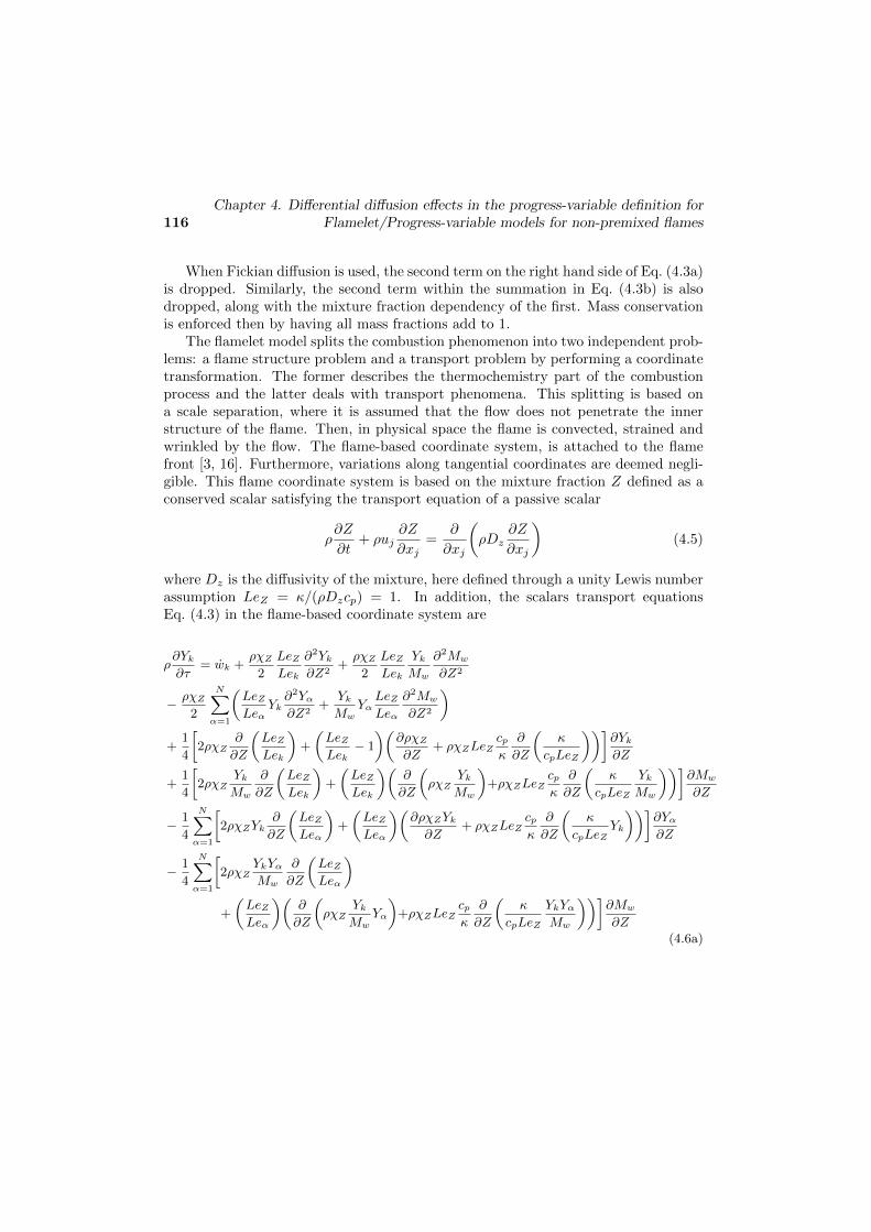
116Chapter 4. Differential diffusion effects in the progress-variable definition for
Flamelet/Progress-variable models for non-premixed flames
When Fickian diffusion is used, the second term on the right hand side of Eq. (4.3a)is dropped. Similarly, the second term within the summation in Eq. (4.3b) is alsodropped, along with the mixture fraction dependency of the first. Mass conservationis enforced then by having all mass fractions add to 1.
The flamelet model splits the combustion phenomenon into two independent prob-lems: a flame structure problem and a transport problem by performing a coordinatetransformation. The former describes the thermochemistry part of the combustionprocess and the latter deals with transport phenomena. This splitting is based ona scale separation, where it is assumed that the flow does not penetrate the innerstructure of the flame. Then, in physical space the flame is convected, strained andwrinkled by the flow. The flame-based coordinate system, is attached to the flamefront [3, 16]. Furthermore, variations along tangential coordinates are deemed negli-gible. This flame coordinate system is based on the mixture fraction Z defined as aconserved scalar satisfying the transport equation of a passive scalar
ρ∂Z
∂t+ ρuj
∂Z
∂xj=
∂
∂xj
(ρDz
∂Z
∂xj
)(4.5)
where Dz is the diffusivity of the mixture, here defined through a unity Lewis numberassumption LeZ = κ/(ρDzcp) = 1. In addition, the scalars transport equationsEq. (4.3) in the flame-based coordinate system are
ρ∂Yk∂τ
= wk +ρχZ
2
LeZLek
∂2Yk∂Z2
+ρχZ
2
LeZLek
YkMw
∂2Mw
∂Z2
− ρχZ2
N∑α=1
(LeZLeα
Yk∂2Yα∂Z2
+YkMw
YαLeZLeα
∂2Mw
∂Z2
)+
1
4
[2ρχZ
∂
∂Z
(LeZLek
)+
(LeZLek
− 1
)(∂ρχZ∂Z
+ ρχZLeZcpκ
∂
∂Z
(κ
cpLeZ
))]∂Yk∂Z
+1
4
[2ρχZ
YkMw
∂
∂Z
(LeZLek
)+
(LeZLek
)(∂
∂Z
(ρχZ
YkMw
)+ρχZLeZ
cpκ
∂
∂Z
(κ
cpLeZ
YkMw
))]∂Mw
∂Z
− 1
4
N∑α=1
[2ρχZYk
∂
∂Z
(LeZLeα
)+
(LeZLeα
)(∂ρχZYk∂Z
+ ρχZLeZcpκ
∂
∂Z
(κ
cpLeZYk
))]∂Yα∂Z
− 1
4
N∑α=1
[2ρχZ
YkYαMw
∂
∂Z
(LeZLeα
)+
(LeZLeα
)(∂
∂Z
(ρχZ
YkMw
Yα
)+ρχZLeZ
cpκ
∂
∂Z
(κ
cpLeZ
YkYαMw
))]∂Mw
∂Z(4.6a)

4.2. Mathematical model 117
ρ∂T
∂τ=ρχZ
2LeZ
∂2T
∂Z2− 1
cpqR − 1
cp
N∑k=1
wkhk +ρχZ
2
LeZcp
∂cp∂Z
∂T
∂Z
+1
4
[2ρχZ
∂Lez∂Z
+ (LeZ − 1)
(∂ρχZ∂Z
+ ρχZLeZcpκ
∂
∂Z
(κ
cpLeZ
))]∂T
∂Z
−N∑k=1
ρχZ2
LeZLek
(∂Yk∂Z
+YkMw
∂Mw
∂Z
)(1− cp,k
cp
)∂T
∂Z
(4.6b)
where χ is the scalar dissipation rate, which introduces flow effects into the flameletspace, and is defined afterwards. When Fickian diffusion is considered and equaldiffusivities are taken for all species Lei = LeZ , the flamelet equations reduce to
ρ∂Yk∂t
= wk +ρχZ
2
∂2Yk∂Z2
(4.7a)
ρ∂T
∂t=ρχZ
2
∂2T
∂Z2− 1
cpqR +
1
cp
N∑k=1
wkhk −ρχZ
2
(1
cp
∂cp∂Z
∂T
∂Z+
N∑k=1
∂Yk∂Z
(1− cp,k
cp
)∂T
∂Z
)(4.7b)
In contrast, the flamelet equations based on the Shvab-Zeldovich formulation, withequal diffusivities and using a coupling function based on, the fuel and oxidiser massfraction or a local element balance, results in
ρ∂Yk∂t
=ρχZ
2
∂2Yk∂Z2
+ wk (4.8a)
ρ∂T
∂t=ρχZ
2
∂2T
∂Z2− 1
cpqR − 1
cp
N∑k=1
wkhk (4.8b)
which is equivalent to Eq. (4.7) if all species heat capacities are equal and constant.In order to study the influence of differential diffusion, results from Eq. (4.6),
the differential diffusion model, and Eq. (4.8), the Fickian model, are compared.Moreover, the “extended” Fickian model, Eq. (4.7), is used to characterise changescaused by variable heat capacities.
The sets of equations Eq. (4.6), (4.7) or (4.8) are function of the mixture fractionand the scalar dissipation rate, which is a central element in the coordinate trans-formation as it represents flow effects in the flame structure problem. It is definedas
χZ = 2DZ
(∂Z
∂xi
∂Z
∂xi
)(4.9)
and has dimension of the inverse of time [1/s], usually regarded as a characteristicdiffusion time.

118Chapter 4. Differential diffusion effects in the progress-variable definition for
Flamelet/Progress-variable models for non-premixed flames
As the scalar dissipation rate is defined as a function of the mixture fraction,once the mixture fraction field in physical space is known, it can be computed. Thisapproach requires a coupled strategy to solve the flamelet equations, which in turnmeans that the flamelet equations have to be solved during CFD computations.
Alternatively, Peters [2] showed that diffusion flames in the flamelet regime may beviewed as counter-flow flames or unsteady mixing layers. From the analytic solutionand asymptotic analysis of those one-dimensional diffusion flames, an expression wasobtained [2, 16],
χZ(Z) =a∞π
Φexp(−2[erfc−1(2Z)]2
)= χst
Φ
Φst
f(Z)
fst(Z)(4.10)
where a∞ is the nominal strain rate in a counter-flow configuration or an inverse ofthe decaying time of an unsteady mixing layer. χst is the scalar dissipation rate atthe stoichiometric mixture fraction χst = χZ |Z = Zst. The function erfc−1 is theinverse of the complementary error function.
In the right hand side (r.h.s.) of Eq. (4.10), f(Z) represents the exponential term,and Φ is a coefficient which accounts for variable density effects [3, 17] and takes theform
Φ =3
4
(√ρ∞/ρ(Z) + 1)2
2√ρ∞/ρ(Z) + 1
(4.11)
where ρ∞ represents the density at the oxidiser side.The last form of Eq. (4.10) is motivated by the interest to express χZ as a function
of a parameter independent of the mixture fraction. Therefore, the scalar dissipationrate is related to its stoichiometric value, which ranges from χst → 0 to χq, the latterrepresenting the scalar dissipation rate at which the flame is quenched. The limit ofzero scalar dissipation rate represents an unstrained diffusion flame. However, theflamelet equations cannot reproduce this limit, because unstrained one dimensionaldiffusion flames become choked by their combustion products.Hence, solutions areusually obtained down to a numerical zero.
Taking advantage of this analogy, a functional form for the scalar dissipation rateis prescribed, which allows solving the flamelet equations in a preprocessing stage.
4.2.1 Flamelet/Progress-variable (FPV) model
The classical flamelet model requires solving the flamelet equations during CFDsimulations due to the presence of the temporal term. Furthermore, since the coor-dinate transformation is attached to the flame front, the temporal timescale τ is aLagrangian-like coordinate [18, 19], which requires the computation of a flamelet La-grangian time and consequently limited the model applicability to simple geometries.Additionally, use of large chemical mechanisms is limited by computational resources.Dropping the temporal dependency, thus considering the flamelet equations in their

4.2. Mathematical model 119
steady state, allows a database to be created in a preprocessing stage and accessingit during CFD simulations. In turn, this introduced an additional scale separation,a temporal one. Chemistry is then assumed to be faster than the characteristic flowtime, relaxing to its steady state in a sufficiently fast time-scale.
Solutions of the flamelet set of equations in their adiabatic steady form can beparametrised by means of the mixture fraction Z and the scalar dissipation rate atstoichiometric mixture fraction χst. Therefore, a two parameter representation ofthe flamelet space is obtained. Plotting the temperatures at stoichiometric mixturefraction Tst as a function of the stoichiometric scalar dissipation rate χst results in therepresentative S-shaped curve for diffusion flames. The reader is referred to Fig. 4.2in Sec. 4.3 and Fig. 4.14 in Sec. 4.4 for the curves of the two cases here studied.
A database of steady flamelets using solely Z and χst can only represent theupper branch of the S-shaped curve, which limits the applicability of the model. Thesteady model projects vertically all solutions under the stable burning branch to it.Therefore, mixing at χst < χq always led to an ignited mixture. The unsteady model,which is capable of representing all states, required solving the flamelet equationsinteractively during CFD simulations.
Pierce and Moin [4] proposed changing χst as a parameter in favour of a progress-variable c to represent steady flamelets. Hence, it would be possible to fully charac-terise the S-shaped curve and consequently being able to describe partially-extinguishedor partially-ignited states. Therefore, this progress-variable must uniquely identifyeach flamelet within the database. Its actual definition will be discussed once themodel and, requirements on the parameter, have been presented. As stated, its defi-nition is found to be case dependent [6–10].
As similarly done for the scalar dissipation rate, the parameter substituting thestoichiometric scalar dissipation rate is the progress-variable at the stoichiometricmixture fraction Λ = c|Zst. This definition is based on the same arguments forusing χst instead of χZ . With it, the three branches of the S-shaped curve can beuniquely characterised. However, use of Λ during CFD simulations has been shown tobe complex, as its transport equation for turbulent flows requires modelling complexunclosed terms. Hence, it is more convenient to use the progress-variable itself asa parameter. Therefore a bijective relation between Λ and c is required in order toproperly define the flamelet space
Λ = ζ−1(Z, c) (4.12)
In the steady Flamelet/Progress-variable (SFPV) model, all the precomputed ther-mochemical variables, including thermophysical quantities and reaction rates, arestored into a database, which is accessed during CFD simulations. The database isthen treated as an equation of state (EoS)
φ = ρ, wc, DZ , ... = zSFPVφ (Z, c) (4.13)

120Chapter 4. Differential diffusion effects in the progress-variable definition for
Flamelet/Progress-variable models for non-premixed flames
If transient terms are retained, in the classical flamelet model, the flamelet equa-tions would have to be solved during CFD simulations in order to account for thetime scale τ in the flamelet equations. With the parameter change, the transientevolution at each χst can be tracked using the progress-variable [5, 20]. Hence, theprogress-variable must be a monotonically varying magnitude. The set of solutionsof the unsteady model becomes a function of the mixture fraction Z, the progress-variable c and the stoichiometric scalar dissipation rate χst. Thus, the database forthe unsteady flamelet can be computed in a preprocessing stage. The EoS for the un-steady Flamelet/Progress-variable (UFPV) adds the stoichiometric scalar dissipationrate to the steady one
φ = ρ, wc, DZ , ... = zUFPVφ (Z, c, χst) (4.14)
Both steady and unsteady FPV databases are generated under the assumption ofadiabatic heat transfer, i.e. without radiative heat loses. Thermal radiation effectsare relevant at high temperatures, which translates into radiation playing a signifi-cant role near the stable burning branch of the S-shaped curve. However, radiationeffects, and similarly NO formation, are slow processes which are not well representedby steady flamelet models. It is assumed that flamelets relax to steady form in suf-ficiently short timescales. As proposed by Ihme and Pitsch [21], starting from theadiabatic steady state solution at the burning branch, transient flamelets at constantχst are computed, where the temperature of the mixture is decreased due to thermalradiation, modelled through an Optically Thin model (OTM) [16, 22]. The enthalpyat stoichiometric mixture fraction H = h|Zst is introduced as parameter, where h isthe total enthalpy, defined as the sum of chemical and sensible enthalpies. As donefor Λ, the enthalpy itself is used rather than the enthalpy parameter. Therefore, abijective relation between h and H is required. Solutions at different stoichiomet-ric scalar dissipation rates define the radiation subspace of the flamelet, which areparametrised as a function of the mixture fraction Z, the progress-variable c and thetotal enthalpy h. An example of the radiation flamelet space may be seen in Fig. 4.9of Sec. 4.3.4. Based on the EoS of the steady FPV plus the enthalpy, the EoS for theradiation Flamelet/Progress-variable (RFPV) is
φ = ρ, wc, DZ , ... = zRFPVφ (Z, c, h) (4.15)
Progress-variable definitionThe FPV model relies on a progress-variable which uniquely identifies each solu-
tion included into the database. Several restrictions are to be taken into account inits definition. Above all, the progress-variable should uniquely characterise the ther-mochemical state and its reaction rate should be non-negative, so that, the progress-variable evolves from an initial state to a final state. Additionally, the species used

4.2. Mathematical model 121
should evolve on comparable timescales and their mass fractions have comparablemagnitudes, in order to avoid the use of large weights.
The progress-variable has been usually defined as a summation of different speciesmass fractions, c =
∑k Yk. Several definitions may be found in the literature with
regard to the actual species considered in this definition. Usually a combination ofCO2, H2O, CO and H2 mass fractions is used. Likewise, the progress-variable maybe defined as a weighted summation c =
∑k ωkYk. Pierce and Moin [4] defined it as
a linear combination of CO2 and H2O, Vreman et al. [8] and Oijen and de Goey [23],in the context of premixed flames, included H2 into the definition and used as weightsthe inverse of the molar mass. Domingo et al. [9], also for premixed flames, used acombination of only CO and CO2. Ihme et al. [20, 21] used the four major species,as well as analysing the effect of the definition on its monotonicity and proposing anoptimisation method for finding the coefficients of each specie, so that the bijectiverelation in Eq. (4.12) was met [10]. The method showed improvements over exist-ing definitions. However, results still showed non-bijective regions. In addition, adependency on the combustion mode, premixed or non-premixed, the chemical mech-anism and considered fuel was shown. In non-premixed flames, diffusion, or mixing,is the rate controlling mechanism of the flame. Usually, a Fickian approximation ismade, which simplifies the computations. However, accounting for differential diffu-sion modifies the species distribution. Therefore, definitions suitable for the Fickianmodel may not be extrapolated to the differential diffusion model.
In this work, the definition of the progress-variable is restricted to two definitions,one considering only CO2 and H2O, denoted as CD1, cCD1 = YCO2
+ YH2O, and asecond one considering CO2, H2O, CO and H2, denoted CD2, cCD2 = YCO +YCO2
+YH2 + YH2O. It will be shown that in some cases it may be interesting to expand thisdefinition by introducing other species or using different weights. However, establish-ing the optimal values for the coefficients would require an optimisation procedurewhich exceeds the aim of the present work.
Since the progress-variable is taken as a summation of species mass fractions, thetransport equation to be computed in physical space is a linear summation of thetransport equation of the different species
ρ∂c
∂t+ ρuj
∂c
∂xj=
∂
∂xj
(ρDc
∂c
∂xj
)(4.16)
where Dc is the progress-variable diffusivity, which is taken equal to the mixturefraction diffusivity. The transport equation of the progress-variable is used in itsFickian form for two reasons.
First, and foremost, differential diffusion effects are important when differentspecies diffuse at different speeds [3, 24]. Since the progress-variable is defined asa combination of species, and most of them present low sensitivity to differential

122Chapter 4. Differential diffusion effects in the progress-variable definition for
Flamelet/Progress-variable models for non-premixed flames
diffusion, these effects become negligible compared to Fickian diffusion. That is, dif-fusion due to species gradients is the dominant term for the progress-variable. Fig. 4.1shows the different terms of Eq. (4.6a) in mixture fraction space for the CH4/H2/N2
diffusion flame. As it can be seen in Fig. 4.1a, differential diffusion terms, 5th and6th terms on r.h.s of Eq. (4.6a), play a significant role for H2. However, for specieswith Lewis number close to 1 the effect is much more limited, as shown for H2O inFig. 4.1b. Therefore, diffusion due to species mass fractions gradients, 2nd term, andthe reaction rate are the leading terms for the progress-variable, as shown in Fig. 4.1cand 4.1d.
-0.2
-0.15
-0.1
-0.05
0
0.05
0.1
0.15
0.2
0.25
0 0.1 0.2 0.3 0.4 0.5 0.6 0.7 0.8 0.9 1
Transport Term [kg/(m3s)]
Z
1st termReaction rate
3rd termDifferential diffusion
Correction Velocity
(a) H2
-1.5
-1
-0.5
0
0.5
1
1.5
0 0.1 0.2 0.3 0.4 0.5 0.6 0.7 0.8 0.9 1
Transport Term [kg/(m3s)]
Z
1st termReaction rate
3rd termDifferential diffusion
Correction Velocity
(b) H2O
-2
-1.5
-1
-0.5
0
0.5
1
1.5
2
0 0.1 0.2 0.3 0.4 0.5 0.6 0.7 0.8 0.9 1
Transport Term [kg/(m3s)]
Z
1st termReaction rate
3rd termDifferential diffusion
Correction Velocity
(c) cCD1 = YCO2+ YH2O
-1.5
-1
-0.5
0
0.5
1
1.5
0 0.1 0.2 0.3 0.4 0.5 0.6 0.7 0.8 0.9 1
Transport Term [kg/(m3s)]
Z
1st termReaction rate
3rd termDifferential diffusion
Correction Velocity
(d) cCD2 = YCO + YCO2+ YH2
+ YH2O
Figure 4.1: Transport terms in the r.h.s of Eq. (4.6a). Results correspond to thestable branch at χst = 1. The fuel is a mixture of H2 and CH4, corresponding tothe DLR flame [13, 14]. Diffusion due to mass fraction gradients are denoted as“1st term”, and due to molar mass gradients as ”3rd term”. Differential diffusionaccounts for the 5th and 6th terms. Correction Velocity includes the 4th, 7th and8th terms. Results were obtained using the GRI3.0 chemical mechanism.

4.2. Mathematical model 123
Second, the correction terms involve all species. Hence, the computational require-ments would considerably increase if the correction terms were included, because itwould entail retrieving all species from the flamelet database during CFD simulations.
4.2.2 Numerical method
Two numerical codes are used in this work. For the flamelet database generationa high order one dimensional code is used. CFD simulations are performed using thegeneral purpose unstructured and parallel object-oriented CFD code TermoFluids[25].
Flamelet databaseIn order to build the flamelet database, the set of equations Eq. (4.6), or alter-
natively their Fickian counterparts Eq. (4.7) or Eq. (4.8), are solved using a onedimensional finite differences code. First and second order derivatives are evaluatedusing 4th order centred approximations. Meshes are refined near the stoichiometricmixture fraction in order to correctly capture the reaction zone. Boundary conditionsare imposed as Dirichlet boundary conditions. At Z = 0 and Z = 1 oxidiser and fuelspecies and temperatures are set, respectively.
Solution of the flamelet equations in their steady form is performed by means ofa Newton Method. The resulting matrix system is solved by means of a sparse LUsolver. The resulting solutions define the S-shaped curve.
Transient solution of the flamelet equations, for both unsteady and radiation mod-els, are performed by means of an Implicit/Explicit Runge-Kutta Scheme (IMEXRKC) [26]. The stiff chemical reaction term is treated implicitly, whereas all diffu-sive terms are treated explicitly. The scheme allows for a variable time-step, whichbecomes a function of the allowed local truncation error at each step and the numberof iterations per step. The advantage of an hybrid explicit-implicit scheme is thatit only requires solving locally implicit systems of equations, as the diffusive term istreated explicitly. The implicit set of equations for the stiff chemical reaction term issolved using an sparse LU solver.
Due to the coordinate change, the flame structure is solved in a flame based coor-dinate system. Therefore, radiation heat losses have to be computed without spatialdependencies. Furthermore, the medium is assumed optically thin. The OpticallyThin model (OTM) assumes that self-absorption is negligible compared to emission[16, 22]. Therefore, each control volume has an unimpeded view of the surrounding,viewed as a black body. Thus, the radiation flux is modelled as control volume heatloss, and is evaluated as
qR = 4σ
(T 4
N∑k=1
(pkkPk)− T 4s
N∑k=1
(pkkIk)
)(4.17)
where σ is the Stefan-Boltzmann constant, pk is the partial pressure of the kth species,

124Chapter 4. Differential diffusion effects in the progress-variable definition for
Flamelet/Progress-variable models for non-premixed flames
kPk and kIk are the Planck-mean and incident-mean absorption coefficients and Tsis the background temperature. Absorption coefficients obtained from RADCAL [27]have been fitted to polynomials of the temperature. The radiant species consideredare CO2, H2O, CH4 and CO.
CFD simulationsThe set of equations Eq. (4.1), (4.2), (4.5) and (4.16) are solved using a finite
volume approach. Particularly, general 3D collocated meshes, either structured orunstructured are used. In order to preserve kinetic energy, a Symmetry-Preservingscheme [28] is used in the construction of the discrete convective term of the momen-tum equation. For the scalar convective terms, a SMART scheme is used [29]. Asecond order centred difference scheme is used to construct the discrete diffusive termfor all transported quantities. Temporal integration is performed using a linear multi-step method, as described in Chapter 2, with a second order Adams-Bashforth in thepredictor step and a Crank-Nicholson scheme in the corrector step. The pressure-velocity coupling is solved by means of a Fractional Step method.
Regarding boundary conditions, scalars are fixed at the inlet boundaries throughDirichlet conditions. In addition, the experimental fuel inflow, in both analysedflames, was reported to behave as a fully developed turbulent pipe flow. There-fore, a fully developed pipe flow is assumed for the turbulent fuel jet in the presentsimulations. Hence, a loosely coupled strategy has been carried out in order to re-produce the experimental inlet conditions. First, in a preprocessing stage a turbulentpipe flow, at the fuel inlet conditions, is simulated and stored. After, during CFDsimulations, at each time-step, velocities are retrieved. Neumann conditions are setfor the velocity at the exit plane.
4.3 Turbulent diffusion CH4/H2/N2 flame - DLR A flame
The first case of study is the CH4/H2/N2 jet flame referred as DLR Flame A[13, 14]. It consists of a Dj = 8mm wide jet with a thinned rim at the exit. The innerjet is composed of 33.2% H2, 22.1% CH4, and 44.7% N2 by volume and the outerjet is regular air with 20.1% O2. The cold jet exit bulk velocity is fixed to 42.15m/sresulting in a Reynolds number of 15, 200. The jet was mounted concentrically to thecoflow nozzle, which had a diameter of 140mm and provided air at 0.3m/s. Both fueland coflow air were at 300K. The stoichiometric mixture fraction is Zst = 0.167. Thepresent flame is stabilised by shear between fuel and oxidiser streams. Thus, propermodelling of the mixing process is critical. As there is a significant amount of hy-drogen in the fuel stream, it has been shown experimentally [13, 14] and numerically[30] that differential diffusion plays a significant role. Due to the presence of H2 insignificant proportions, this case will serve to assess how the progress-variable defi-nition is affected when differential diffusion is included. First, the flamelet database

4.3. Turbulent diffusion CH4/H2/N2 flame - DLR A flame 125
is analysed to assess the effect of the diffusion model and the chemical mechanism.Then, results of CFD simulations are presented.
4.3.1 Flamelet burning region - Fickian vs Differential
First the flamelet accessible subspace is analysed using the S-shaped curve. Whendifferential diffusion is accounted for, a twofold effect on the flamelet burning regionis shown in Fig. 4.2: it produces an increase in the temperatures of the stable branchof the curve and it increases the scalar dissipation rate at extinction χq. This temper-ature increase also translates into higher heat fluxes between burned and unburnedmixtures. Part of this increase is also attributable to gradients of the heat capacity.The reason for this influence is explained by the significant difference in heat capac-ities between fuel and oxidant species. Nonetheless, differential diffusion enables theflame to sustain higher scalar dissipation rates without extinguishing. In the unstablebranch it can be seen a convergence between both models between χst = 1 and 10.Afterwards, the curves diverge again. In any case, accounting for differential diffusionresults in the ignition region of the S-shaped beginning at lower temperatures. Thus,igniting flamelets are found at slightly lower temperatures. In this region, the effectof the heat capacity is limited when compared to its effect on the upper branch.
Comparing the two chemical mechanisms, GRI2.11 against GRI3.0, there is asmall effect in the accessible regions of the flame. For the GRI2.11, the extinctionscalar dissipation rate is marginally increased and temperatures at the stoichiometricmixture fraction are slightly decreased. Therefore, no significant differences betweenboth mechanisms with regard to the ignition and extinction of the flame for thisconfiguration is expected. Nonetheless, it is interesting to note that at the smallestχst of the stable branch, the effect of the chemical mechanisms is almost negligible,whereas close to χq the effect is small but noticeable. Along the unstable branch, asimilar effect is observed.
4.3.2 Progress-variable definition - steady
The FPV model assumes a bijective relation between the progress-variable atthe stoichiometric mixture fraction, Λ, and the progress-variable, c, at each mixturefraction. Consequently, the progress-variable must be a monotonic function, rangingbetween the extinguished state and the steady stable burning solution.
In Fig. 4.3 are shown the progress-variable values obtained from the steady flameletequations with differential diffusion at different stoichiometric scalar dissipation ratesas a function of the mixture fraction for the two definitions considered. It can beseen that the progress-variable parameter Λ is monotonic in all cases. Regardingthe considered definitions, it can be seen that neither CD1 nor CD2 result in abijective relation. Furthermore, CD1 shows overlapping regions around the stableand unstable regions. In the former, near Zst at low χst and for the latter at highmixture fraction regions CD2 improves the definition in both branches. At the stable

126Chapter 4. Differential diffusion effects in the progress-variable definition for
Flamelet/Progress-variable models for non-premixed flames
0
400
800
1200
1600
2000
2400
0.1 1 10 100 1000
Tst [K]
χst [s-1]
DD-GRI3.0
Fick-GRI3.0
Fick Ext-GRI3.0
Fick-GRI2.11
DD-GRI2.11
Figure 4.2: S-shaped curve for a CH4/H2/N2 diffusion jet flame. Curves withdifferential diffusion effects are denoted by DD.
branch is monotonic except at low χst. The smallest included χst is 0.1, and it hasbeen seen that up to χst = 0.2, CD2 definition is bijective, see the inset in Fig. 4.3b.
Concerning the chemical mechanism, there is a slight difference at the unstablebranch, where the GRI2.11 manifests a smaller overlapping than the GRI3.0. How-ever, at the stable branches when the GRI2.11 is used there is a slight overlapping atintermediate scalar dissipation rates χst = [1, 10]. On the contrary, the GRI3.0 doesnot manifest this behaviour.
If Fickian diffusion is used, shown in Fig. 4.4, and considering CD2 definition,Eq. (4.12) is bijective at the stable branch for both mechanisms. However, the unsta-ble branch is poorly represented, as there is a large overlapping of solutions at highmixture fraction values. CD1 definition results in a better description of the unstablebranch. Nonetheless, it is not monotonic. Furthermore, a marked non-monotonicregion is observed around the stable branch at the rich side of the flame. Consideringthe chemical mechanism, similar trends are observed in both cases.
The overlap at the unstable branch is found at small χst as the peak of theprogress-variable is displaced from values close to Zst to values closer to Z = 0.5,which is the point where the scalar dissipation peaks. Both diffusion models featuresimilar effects regarding the flamelets profiles.
Considering the extended Fickian flamelet equations, Eq. (4.7), for the speciesdistributions around the stable branch no significant differences with respect to thebaseline results are observed. Differences are found in the temperature profiles at

4.3. Turbulent diffusion CH4/H2/N2 flame - DLR A flame 127
0
0.05
0.1
0.15
0.2
0.25
0 0.2 0.4 0.6 0.8 1
c=YCO2+YH2O
Z
Zst
χst
χst
Stable Branchχq
Unstable BranchMixing line
0.185
0.19
0.195
0.2
0.12 0.15 0.18 0.21 0.24
(a) GRI3.0 CD1
0
0.05
0.1
0.15
0.2
0.25
0 0.2 0.4 0.6 0.8 1
c=YCO+YCO2
+YH2
+YH2O
Z
Zst
χst
χst
0.225
0.23
0.18 0.21 0.24
(b) GRI3.0 CD2
0
0.05
0.1
0.15
0.2
0.25
0 0.2 0.4 0.6 0.8 1
c=YCO2
+YH2O
Z
Zst
χst
χst
0.185
0.19
0.195
0.2
0.12 0.15 0.18 0.21 0.24
(c) GRI2.11 CD1
0
0.05
0.1
0.15
0.2
0.25
0 0.2 0.4 0.6 0.8 1
c=YCO+YCO2
+YH2
+YH2O
Z
Zst
χst
χst
0.225
0.23
0.18 0.21 0.24
(d) GRI2.11 CD2
Figure 4.3: Progress-variable definition for a steady laminar flamelet using differ-ential diffusion. Arrows indicate increasing χst. Note that the legend applies onlyto the big plot, the inset line-styles are set to distinguish between different curvesof the stable branch.
the unstable branch. For the base Fickian diffusion model, past the stoichiometricmixture fraction, the temperature profile is curved instead of a straight line due tothe presence of the heat capacity gradients. Regarding the “extended” one, it can beseen in Fig. 4.5 that the overlapping regions are greatly reduced. However, includingCO and H2, CD2 definition, causes overlapping regions to reappear. Therefore, theoverlap reduction seen in the differential diffusion model is basically due to heatcapacity gradients term in the flamelet equations.
Overall, there is a competing effect in the progress-variable definition when in-cluding H2 and CO. On the one hand, including them improves the mapping of theflamelet solutions around the upper branch. On the other hand, these species causethe opposite effect around the unstable branch. However, when differential diffusion

128Chapter 4. Differential diffusion effects in the progress-variable definition for
Flamelet/Progress-variable models for non-premixed flames
0
0.05
0.1
0.15
0.2
0.25
0 0.2 0.4 0.6 0.8 1
c=YCO2
+YH2O
Z
Zst
χst
χst
0.195
0.205
0.215
0.15 0.18 0.21 0.24
0.08
0.1
0.3 0.4 0.5
(a) GRI3.0 CD1
0
0.05
0.1
0.15
0.2
0.25
0 0.2 0.4 0.6 0.8 1
c=YCO+YCO2
+YH2
+YH2O
Z
Zst
χst
χst
0.225
0.23
0.235
0.18 0.21 0.24
(b) GRI3.0 CD2
0
0.05
0.1
0.15
0.2
0.25
0 0.2 0.4 0.6 0.8 1
c=YCO2+YH2O
Z
Zst
χst
χst
Stable Branchχq
Unstable BranchMixing line
0.18
0.20
0.22
0.18 0.21 0.24
0.08
0.1
0.3 0.4 0.5
(c) GRI2.11 CD1
0
0.05
0.1
0.15
0.2
0.25
0 0.2 0.4 0.6 0.8 1
c=YCO+YCO2
+YH2
+YH2O
Z
Zst
χst
χst
0.225
0.23
0.235
0.18 0.21 0.24
(d) GRI2.11 CD2
Figure 4.4: Progress-variable definition for a steady laminar flamelet using Fickiandiffusion. See comments of Fig. 4.3 for further details.
is considered, the overlapping is less pronounced. With CD2, a smoother evolutionof the progress-variable in the upper curve region is observed using Fickian diffusion.On the contrary, the differential diffusion model results into a more cramped flameletsolution, see insets in Fig. 4.3b, 4.3d, 4.4b and 4.4d. If each specie is analysed sep-arately, it is observed that CO2 curves overlap near the stable branch, whereas theH2O ones overlap near the unstable branch. H2 and CO feature complex evolution.It is then difficult to manually find an optimal definition for the progress-variable.A coefficient optimisation, which could include other minor species, such as the oneproposed by Ihme et al. [10] or similar, would be required to obtain a fully bijectiverelation. Nevertheless, CFD results to be presented in the following sections showthat CD2 with minor modifications is adequate for the current case. Alternativedefinitions using mainly major species, such as c = YCO + YCO2
, result also, for thepresent case, in Eq. (4.12) being non-monotonic.

4.3. Turbulent diffusion CH4/H2/N2 flame - DLR A flame 129
0
0.05
0.1
0.15
0.2
0.25
0 0.2 0.4 0.6 0.8 1
c=YCO2
+YH2O
Z
Zst
χst
χst
0.18
0.2
0.22
0.15 0.18 0.21 0.24
(a) GRI3.0 CD1
0
0.05
0.1
0.15
0.2
0.25
0 0.2 0.4 0.6 0.8 1
c=YCO+YCO2+YH2+YH2O
Z
Zst
χst
χst
Stable branchχq
Unstable branchMixing line
0.23
0.232
0.234
0.18 0.21 0.24
(b) GRI3.0 CD2
Figure 4.5: Progress-variable definition for a steady laminar flamelet using theextended Fickian diffusion. See comments of Fig. 4.3 for further details.
Fig. 4.3 and 4.4 also depict the difference in ignited regions seen in Fig. 4.2. Thedifferential diffusion model features a larger region of ignited solutions and conse-quently, larger ignited reaction rates. This will be shown to have direct consequencesduring CFD simulations. Additionally, at the unstable branch as χst is reduced, asubtle effect of the diffusion model can be seen in the figures. For both models, a χstreduction results in a lower value of the flamelet maximum progress-variable and adisplacement of this maximum towards Z = 0.5, where the maxima of the χ distri-bution is located. CD1 shows a similar trend for both diffusion models, where CO2
and H2O mass fractions are reduced. However, CD2 shows interesting differences.It can be seen that there is a local minimum for all cases. On the one hand, forflamelets with the GRI3.0 mechanism, the flamelet maximum does not change. Onthe other hand, the GRI2.11 shows a continuous decrease after going through a localmaximum. Thus, highlighting differences in H2 and CO predictions between chemi-cal mechanisms at intermediate temperatures. The just described phenomenon is notfully captured by the the S-shaped curve.
4.3.3 Progress-variable definition - unsteady
When the unsteady FPV model is considered, the scalar dissipation rate at sto-ichiometric mixture fraction is used as an additional parameter. Therefore, theprogress-variable follows the ignition/extinction process of the mixture at a constantχst. Hence, the monotonic evolution of the progress-variable is evaluated at each χstindependently.
For the unsteady flamelets with differential diffusion, no significant differences,regarding the monotonic growth of the progress-variable are observed between CD1or CD2. In both cases the progress-variable is non-monotonic as the ignition process

130Chapter 4. Differential diffusion effects in the progress-variable definition for
Flamelet/Progress-variable models for non-premixed flames
approaches the stable solution, as shown in Fig. 4.6 for CD2. However, if the massfraction of C2H2 is added to the summation, with a coefficient of 5, the resultingdefinition is monotonic, excepting for the lowest χst = 0.1. However, at χst = 0.5,the definition is bijective. It should be noted, that the resulting reaction rate ofthe progress-variable is not always positive. Near the stable solution, the reactionrate becomes slightly negative. The use of minor species with a large coefficient isrequired since major product species account for most of the mass fraction near thestable branch. Alternatively, a combination of the major product species, CO, CO2,H2 and H2O using a non-trivial set of coefficients could probably result in a uniquelymapping of the flamelet evolution at each χst. Nonetheless, the proposed approach,which is to add C2H2, is viable if the range of flamelets is limited to χst ≥ 0.5.
Concerning the chemical mechanisms, no noticeable differences regarding the mono-tonic growth of the progress-variable are observed between them. Therefore, onlyresults with the GRI3.0 are shown. As the stoichiometric scalar dissipation rate isincreased, lower overlapping is found.
Unsteady flamelets with Fickian diffusion are correctly described using CD1 def-inition for the progress-variable at all χst, as shown in Fig. 4.7. Addition of H2 andCO results in a non-monotonic evolution for χst ≤ 10, as it can be seen in Fig. 4.7aand Fig. 4.7b for CD2 definition. Addition of C2H2 has the same effect in correctingCD2 as in the differential diffusion case.
Comparing results from cases with differential and Fickian diffusion, it is foundthat the higher/lower mobility of light/heavy species results in a modified pool ofreactants during the transient ignition. This leads to a larger local production ofCO2 and H2O, which afterwards diffuses, causing the non-monotonic evolution as thepeak is reduced. On the other hand, with the Fickian diffusion model, created speciesdiffuse at enough speed so as not to build-up a large pool of products. Focusing on thecases at low χst, when Fickian diffusion is considered, ignition is seen to start aroundthe peak of the unstable branch and as the mixture reacts it diffuses heat and reactantssimultaneously up to the equilibrium values. However, when differential diffusion isaccounted for, a narrow reaction zone can be identified, which evolves the progress-variable locally. Then, after the reaction has been completed, it diffuses heat andproducts until the steady state solution is reached, namely the stable branch solution.Comparing the flamelet evolution at high scalar dissipation rates, Fig. 4.6d and 4.7d,it can be seen that they feature similar transitions. This indicates that diffusiondue to species gradients is dominant, thus concealing differential diffusion effects.Comparison of the ignited solutions at χst = 100, Fig. 4.6d and 4.7d, shows that forthe Fickian case the region of ignited solutions is narrower than in the differentialdiffusion case. The reason is that for this χst the Fickian flamelet is closer to theextinction scalar dissipation rate χq than the one with differential diffusion, depictedas the turning point in Fig. 4.2.

4.3. Turbulent diffusion CH4/H2/N2 flame - DLR A flame 131
0
0.05
0.1
0.15
0.2
0.25
0 0.2 0.4 0.6 0.8 1
c=YCO+YCO2
+YH2
+YH2O
Z
Zst
0.22
0.23
0.24
0.16 0.2 0.24 0.28
c=YCO+Y
CO2
+YH2
+YH2O+5*Y
C2H2
(a) χst = 0.1
0
0.05
0.1
0.15
0.2
0.25
0 0.2 0.4 0.6 0.8 1
c=YCO+YCO2
+YH2
+YH2O
Z
Zst
0.22
0.23
0.24
0.16 0.2 0.24 0.28
c=YCO+Y
CO2
+YH2
+YH2O+5*Y
C2H2
(b) χst = 1
0
0.05
0.1
0.15
0.2
0.25
0 0.2 0.4 0.6 0.8 1
c=YCO+YCO2+YH2+YH2O
Z
Zst Mixing lineUnstable branch
Ignition - reactionIgnition - difusion
Stable Branch
0.22
0.24
0.16 0.2 0.24 0.28
c=YCO+YCO2+YH2
+YH2O+5*YC2H2
(c) χst = 10
0
0.05
0.1
0.15
0.2
0.25
0 0.2 0.4 0.6 0.8 1
c=YCO+YCO2
+YH2
+YH2O
Z
Zst
0.2
0.22
0.24
0.16 0.2 0.24 0.28
c=YCO+Y
CO2
+YH2
+YH2O+5*Y
C2H2
(d) χst = 100
Figure 4.6: Progress-variable for unsteady laminar flamelets using differential dif-fusion. The extinction process is not shown as no overlapping of solutions is found.The inset plot shows the non-bijective region using a modified CD2 definition,where the mass fraction of C2H2 is taken into account.
Similarly, in the extinction process, between the unstable branch and the mixingline, which is not shown in the figures, a monotonic evolution of the progress-variableis obtained in all cases, Fickian or differential diffusion, using either CD1 or CD2.
Regarding the progress-variable evolution, a limited influence of the heat capacitygradients is observed. Fig. 4.8 shows the ignition at χst = 0.1 and 1, and it canreadily be seen that they show similar evolutions compared to Fig. 4.7. Therefore,differences between Fickian and differential diffusion models are not attributable toheat capacity gradients.
Compared to the steady FPV model, adding H2 and CO to the progress-variable inthe unsteady FPV model results in non-monotonic evolution near the stable branch ateach χst due to an overproduction of intermediate species. After reaching their peak

132Chapter 4. Differential diffusion effects in the progress-variable definition for
Flamelet/Progress-variable models for non-premixed flames
0
0.05
0.1
0.15
0.2
0.25
0 0.2 0.4 0.6 0.8 1
c=YCO2
+YH2O
Z
Zst
0.22
0.23
0.24
0.16 0.2 0.24 0.28
c=YCO+Y
CO2
+YH2
+YH2O
(a) χst = 0.1
0
0.05
0.1
0.15
0.2
0.25
0 0.2 0.4 0.6 0.8 1
c=YCO2
+YH2O
Z
Zst
0.22
0.23
0.24
0.16 0.2 0.24 0.28
c=YCO+Y
CO2
+YH2
+YH2O
(b) χst = 1
0
0.05
0.1
0.15
0.2
0.25
0 0.2 0.4 0.6 0.8 1
c=YCO2
+YH2O
Z
Zst
0.22
0.23
0.24
0.18 0.21 0.24 0.27
c=YCO+Y
CO2
+YH2
+YH2O
(c) χst = 10
0
0.02
0.04
0.06
0.08
0.1
0.12
0.14
0.16
0.18
0.2
0 0.2 0.4 0.6 0.8 1
c=YCO2+YH2O
Z
Zst
Unstable BranchIgnition
Stable Branch
(d) χst = 100
Figure 4.7: Progress-variable for unsteady laminar flamelets using Fickian dif-fusion. Vertical axis corresponds to CD1, whereas the inset shows the progress-variable around the curve peak using CD2.
value, they recombine into more stable molecules and/or diffuse away. Furthermore,when differential diffusion is taken into account, this peak is more pronounced, whichcan be related to the narrower ignition process observed.
4.3.4 Progress-variable definition - radiation
In order to consider radiation effects, a subset of the flamelet space is considered.The parameters of the database are the mixture fraction, the progress-variable and themixture enthalpy. However, in the following analysis, the definition of the progress-variable is studied independently from the enthalpy because the generation of theflamelet database is performed by means of unsteady flamelets with radiation atconstant χst. Besides, the enthalpy as a function of the mixture fraction is notshown since it is unambiguously defined and its evolution is monotonic. The enthalpy

4.3. Turbulent diffusion CH4/H2/N2 flame - DLR A flame 133
0
0.05
0.1
0.15
0.2
0.25
0 0.2 0.4 0.6 0.8 1
c=YCO2
+YH2O
Z
Zst
0.22
0.23
0.24
0.16 0.2 0.24 0.28
c=YCO+Y
CO2
+YH2
+YH2O
(a) χst = 0.1
0
0.05
0.1
0.15
0.2
0.25
0 0.2 0.4 0.6 0.8 1
c=YCO2
+YH2O
Z
Zst
0.22
0.23
0.15 0.18 0.21 0.24 0.27
c=YCO+Y
CO2
+YH2
+YH2O
(b) χst = 1
Figure 4.8: Progress-variable for unsteady laminar flamelets with extended Fick-ian diffusion model. See Fig. 4.7 for further explanation.
decreases as radiation heat losses increase.Beginning with the accessible burning region, Fig. 4.9 shows that at low χst, the
stable solutions considering radiation tend to similar temperatures at stoichiometricmixture fraction, regardless of the diffusion model. This suggests that when radiationplays a significant role, differences between Fickian and differential difusion becomeless pronounced, even though the adiabatic temperatures are significantly different.The extended Fickian model also follows this trend. Furthermore, as shown in Fig. 4.2,the main difference between the two variants of the Fickian diffusion model is foundat the stable burning branch. Therefore, as in the steady FPV model, part of thedifferences between diffusion models are accountable to gradients of the heat capacity.Regarding the chemical mechanism, the trends are similar for both chemical mech-anisms. Fig. 4.9 is obtained for the GRI3.0, but no significant differences are foundwhen the GRI2.11 is used. This is consistent with the similar behaviour between thetwo mechanism at the stable burning branch for this flame.
In Fig. 4.10 and 4.11 are shown the progress-variable profiles using differentialand Fickian diffusion, respectively. Results are shown for χst = 0.1. Similar trendsare observed at higher scalar dissipation rates. It should be noted that temperaturedecreases from the adiabatic solution to the “radiation” stable solution, which is theflamelet stable solution at a given χst with radiation considered.
First of all, a similar trend, regarding CD1 and CD2, is observed in both dif-ferential and Fickian diffusion models. On the one hand, when CD1 is used, theprogress-variable evolves increasing its value from the steady adiabatic solution tothe steady “radiation” solution, as it can be seen in Fig. 4.10a, 4.10c, 4.11a and 4.11c.On the other hand, using CD2, that is including CO and H2, causes the oppositebehaviour, the progress-variable evolves decreasing its value from the steady adia-

134Chapter 4. Differential diffusion effects in the progress-variable definition for
Flamelet/Progress-variable models for non-premixed flames
0
400
800
1200
1600
2000
2400
0.1 1 10 100 1000
Tst [K]
χst [s
-1]
Adiabatic Stable solution
Radiation Stable Solution
(a) Differential diffusion.
0
400
800
1200
1600
2000
2400
0.1 1 10 100 1000
Tst [K]
χst [s
-1]
Adiabatic Stable solution
Radiation Stable Solution
(b) Fickian diffusion.
Figure 4.9: S-shaped curve depicting the radiation flamelet subspace as the areabetween the adiabatic and ”radiation” curves. Results obtained using the GRI3.0mechanism.
batic solution to the steady “radiation” solution, shown in Fig. 4.10b, 4.10d, 4.11band 4.11d. Albeit this clear trends, no general conclusions can be drawn from it,because the four species feature complex evolutions, changing from increase to de-crease around the stoichiometric mixture fraction, and at some regions close to theoxidiser boundary, which can be inferred from the insets in Fig. 4.10 and 4.11. Fur-thermore, the change of each specie’s mass fraction is different. For example, H2O isthe dominant specie. However, its variation is small compared to CO2, which featuresa larger change (∆YCO2
> ∆YH2O), but its absolute mass fraction is lower than H2O(YH2O > YCO2). Therefore, CD1 mostly tracks H2O mass fraction with the variationsof CO2.
Considering CD1 definition with the differential diffusion model, it can be seenin Fig. 4.10 that it behaves monotonically at almost all mixture fractions. However,there is a small region where Eq. (4.12) is not bijective. Furthermore, addition of H2
and CO, CD2 variant, results in two non-bijective regions. Taking into account theprevious discussion regarding the behaviour of the different species composing CD2,a variant of this definition using different weights for each species has been foundto result in a monotonic evolution of the progress-variable. The new definition isc = 0.5YCO − YCO2
+ YH2+ YH2O and is shown in the inset at the top right corner
of Fig. 4.10b. A minor drawback is that the resulting reaction rate of the progress-variable is slightly negative around the uppermost curve for a small range of mixturefractions.
When Fickian diffusion is considered, use of CD1 results in a large non-bijectiveregion close to Zst. Opposite to the differential diffusion case, CD2 is almost bijective.However, there remains a small non-monotonic region at Z < Zst. The variant used

4.3. Turbulent diffusion CH4/H2/N2 flame - DLR A flame 135
0
0.05
0.1
0.15
0.2
0.25
0 0.2 0.4 0.6 0.8 1
c=YCO2+YH2O
Z
Zst
Adiabatic Stable Branch
Radiative Stable Solution
Transient
0.18
0.2
0.22
0.1 0.11 0.12
(a) χst = 0.1 with CD1 using GRI3.0.
0
0.05
0.1
0.15
0.2
0.25
0 0.2 0.4 0.6 0.8 1
c=YCO+YCO2
+YH2
+YH2O
Z
Zst
0.18
0.2
0.22
0.1 0.11 0.12
0.225
0.23
0.12 0.15 0.18
0.04
0.08
0.12
0.16
0.08 0.12 0.16 0.2
c=0.5YCO-Y
CO2
+YH2
+YH2O
(b) χst = 0.1 with CD2 using GRI3.0. Topright corner inset shows c = 0.5YCO−YCO2
+YH2 + YH2O
0
0.05
0.1
0.15
0.2
0.25
0 0.2 0.4 0.6 0.8 1
c=YCO+YCO2
+YH2
+YH2O
Z
Zst
0.18
0.2
0.22
0.1 0.11 0.12
0.04
0.08
0.12
0.16
0.05 0.1 0.15 0.2 0.25 0.3
c=0.5YCO-Y
CO2
+YH2
+YH2O
(c) χst = 0.1 with CD1 using GRI2.11. Topright corner inset shows c = 0.5YCO−YCO2 +YH2
+ YH2O
0
0.05
0.1
0.15
0.2
0.25
0 0.2 0.4 0.6 0.8 1
c=YCO+YCO2
+YH2
+YH2O
Z
Zst
0.18
0.2
0.22
0.1 0.11 0.12
0.225
0.23
0.12 0.15 0.18
(d) χst = 0.1 with CD2 using GRI2.11
Figure 4.10: Progress-variable for radiation flamelets with differential diffusion.
for the differential diffusion model, in which CO2 had a negative coefficient, does notcorrect the problem in flamelets using the Fickian diffusion model. The reason is againrelated to the evolution of CO2 and H2O, which present different trends when theFickian diffusion model is used. Addition of OH and C2H2 with adequate coefficientsto CD2, c = YCO + YCO2
+ YH2+ YH2O + 5YOH − 0.1YC2H2
, corrects the overlapping.However, similarly to the differential diffusion model, slightly negative reaction ratesat the uppermost curves are obtained.
Regarding the extended Fickian model no significant differences with respect tothe base Fickian model are observed concerning the progress-variable. CD1 showsthe overlapping region around Zst, which CD2 reduces, but does not fully resolve.The variant using OH and C2H2 fixes the overlapping, with the same issues about

136Chapter 4. Differential diffusion effects in the progress-variable definition for
Flamelet/Progress-variable models for non-premixed flames
the reaction rate.
0
0.05
0.1
0.15
0.2
0.25
0 0.2 0.4 0.6 0.8 1
c=YCO2
+YH2O
Z
Zst
Adiabatic Stable Branch
Radiative Stable Solution
Transient
0.2
0.21
0.22
0.15 0.18 0.21
(a) χst = 0.1 with CD1 using GRI3.0.
0
0.05
0.1
0.15
0.2
0.25
0 0.2 0.4 0.6 0.8 1
c=YCO+YCO2
+YH2
+YH2O
Z
Zst
0.2
0.21
0.22
0.23
0.24
0.14 0.16 0.18
0.18
0.2
0.22
0.24
0.14 0.16 0.18 0.2
c=YCO+Y
CO2
+YH2
+YH2O+5*Y
OH-0.1*Y
C2H2
(b) χst = 0.1 with CD2 using GRI3.0. Topright corner inset shows c = YCO + YCO2
+YH2 + YH2O + 5YOH − 0.1YC2H2
0
0.05
0.1
0.15
0.2
0.25
0 0.2 0.4 0.6 0.8 1
c=YCO2
+YH2O
Z
Zst
0.2
0.22
0.15 0.18
(c) χst = 0.1 with CD1 using GRI2.11.
0
0.05
0.1
0.15
0.2
0.25
0 0.2 0.4 0.6 0.8 1
c=YCO+YCO2
+YH2
+YH2O
Z
c=YCO+Y
CO2
+YH2
+YH2O+5*Y
OH-0.1*Y
C2H2
Zst
0.225
0.23
0.235
0.16 0.18 0.2
0.22
0.24
0.14 0.16 0.18 0.2
(d) χst = 0.1 with CD2 using GRI2.11. Bot-tom inset shows c = YCO + YCO2 + YH2 +YH2O + 5YOH − 0.1YC2H2
Figure 4.11: Progress-variable for radiation flamelets with Fickian diffusion.
In addition, no significant differences between chemical mechanisms have beenobserved concerning the monotonic growth of the progress-variable. Still, in Fig. 4.10and 4.11, when the GRI2.11 is used, both definitions of the progress-variable show alarger overlap compared to the GRI3.0. Nonetheless, both mechanisms show similarsensitivity to the diffusion model and progress-variable definition.
As a side note, the flamelet model with heat losses is usually used when slowprocesses, such as radiation or NO formation are of interest. Additionally, it hasbeen reported that the GRI3.0 NO predictions are higher than with the GRI2.11 [12].Comparing NO profiles from flamelets using either mechanism shows 20% differencein peak NO at low χst. However, as stated, no significant differences are observed for

4.3. Turbulent diffusion CH4/H2/N2 flame - DLR A flame 137
major species, which are used to define the progress-variable.
4.3.5 CFD analysis
Large Eddy Simulation (LES) have been performed in order to test the differencesbetween the databases created using Fickian and differential diffusion. The compu-tational domain is 75Dj in the axial direction, with a circular base of 11.5Dj and anupstream base of 31.5Dj . A structured mesh of around 1.9MCV has been used, con-sisting of 645x95x32 nodes in the axial, radial and azimuthal directions, respectively.The mesh has been stretched close to the central jet, where cell size is around 15-20times the Kolmogorov scale. Thus, ensuring that the subgrid scales (sgs) model wasworking in the inertial range. Turbulent fluxes have been modelled using an eddydiffusivity model with the turbulent viscosity evaluated using the WALE sgs model[31].
Up so far, the discussion was centred around the laminar database. However, inLES Favre filtered quantities are obtained from the CFD simulations. Therefore, it isnecessary to restate the database as a function of turbulent Favre-filtered variables.The statistical distributions of the variables used to create the flamelet database arepresumed, allowing to retain the preprocessing advantage of the method. Hence, themixture fraction statistical distribution is modelled using a β-pdf and a δ-pdf for theprogress-variable [4]. The resulting state relation for the SFPV model is then
φ =
∫∫ζφ(Z,Λ)P (Z,Λ)dZdc =
∫∫ζφ(Z,Λ)β(Z; Z, Zv)P (Λ−Λ)dZdΛ = z(Z, Zv, c)
(4.18)where Zv is the subfilter variance of the mixture fraction and a bijective relationbetween Λ and the progress-variable is assumed, as in Eq. (4.12). Evaluation ofsubgrid mixture fraction variance and subfilter scalar dissipation rate is performedthrough a scale similarity model [32], which assumes a local equilibrium betweenproduction and dissipation of the variance at the small scales. When the unsteadyor radiation databases are used, in Eq. (4.18), δ-pdfs are assumed for χst [5, 7] andfor the enthalpy at stoichiometric mixture fraction H = h|Zst [33]. For the latter, aswith the progress-variable, a bijective relation between H = h|Zst and h is assumed.Therefore, the database is parametrised as a function of the latter. For the simulationsincluding radiation heat losses, an OTM is used, computed using Eq. (4.17), as donein the flamelet calculations.
A database with 100x25x100 points in the Z, Zv, c directions was created. Forthe unsteady variant 13 different transient flamelets were considered. The radiationvariant, due to computational limitations, used 75x25x75x65 points in Z,Zv, c and hdirections.
Following the discussion in the previous section, the progress-variable is definedusing the most suitable definition for each flamelet model. The current flame has

138Chapter 4. Differential diffusion effects in the progress-variable definition for
Flamelet/Progress-variable models for non-premixed flames
been reported to be attached to the fuel nozzle and to feature low levels of extinctionand re-ignition. Furthermore, experimental conditional profiles [13] are seen to matchmostly the flamelet profiles of the burning branch. Therefore, for the SFPV, CD2definition is used, since it results in a better description of the stable burning branch.Besides, chemical reactions are mostly taking place at lean mixture fractions. Hence,the overlapping at high mixture fraction values and around the unstable branch shouldhave limited consequences. In order to create the database, in this particular region,the flamelet variables are replaced by a monotonic evolution between the adjacentbijective regions. Computations using the UFPV model use the modified variant ofCD2 with χst > 0.5. Similarly, simulations with the RFPV including differentialdiffusion use CD2 variant with a negative coefficient for CO2.
Instantaneous snapshots of the progress-variable are shown in Fig. 4.12 using thedifferent variants of the FPV model. The SFPV using either Fickian or extendedFickian diffusion models resulted in a flame lift-off and the flame stabilising at around30Dj , where jet velocities are low, as shown in Fig. 4.12a and Fig. 4.12b respectively.Since the Fickian case showed a large non-bijective region at the unstable branch, asimulation was run using CD1 to rule out the progress-variable definition as causefor the flame lift-off. Nonetheless, the flame did also lift-off. When the databaseconsidering differential diffusion was used, flame stabilisation was found closer to thefuel jet nozzle, Fig. 4.12c, and with a shape similar to those of the experiments. Thedifference in stabilisation distance, for the steady FPV model, between Fickian anddifferential diffusion models may be related to the differences in the S-shaped curve,Fig. 4.2. For the latter model, the ignition region begins at lower temperatures, thusthe flame reaches sooner the ignition region, where the reaction rate starts to grownon-linearly. Furthermore, when differential diffusion is considered, the stable branchis located at higher temperatures, which results in higher heat and mass fluxes oncethe mixture has reached the stable burning conditions. Nonetheless, using the SPFVmodel, in all cases the flame lifts-off, which is not in accordance with the experimentalresults. However, differential diffusion shows a significant effect in the stabilisation ofthe flame. Similarly, Chan et al. [34] also found that differential diffusion played asignificant role in the stability of the flame when studying a flame in a jet-in-cross-flow.
Current results using the UFPV model do not show a significant improvementregarding the stabilisation distance. The reason is that the region under the unstablebranch, and focusing on the reaction rate profiles, is similar between the unsteady andsteady FPV variants. Hence, it is not until the progress-variable has increased enough,up to the unstable branch, that differences between both variants are perceptible.This can be observed in Fig. 4.13, where differences between reaction rates profilesat different mixture fractions are shown. Furthermore, experimentally the flame isseen to be immediately ignited, thus it reaches the stable burning branch rapidly.Therefore, transient effects should be of secondary importance and thus, no significant

4.3. Turbulent diffusion CH4/H2/N2 flame - DLR A flame 139
(a) SFPV Fickian. (b) SFPV extendedFickian.
(c) SFPV DD. (d) UFPV DD. (e) Classicalflamelet DD.
Figure 4.12: Instantaneous snapshots of CFD results using different flamelet anddiffusion models. DD indicates differential diffusion. Black indicates the maximumprogress-variable and light-grey indicates a zero progress-variable. The domainshown has been clipped for plotting purposes. Dimensions have been made non-dimensional using the fuel nozzle diameter Dj .
differences would be expected between steady and unsteady models.An important aspect to consider is that the assumed pdf for the progress-variable
can limit the effectiveness of the model. A δ-pdf assumption implies that a particu-lar control volume can be characterised by a single flamelet. Plotting the progress-variable reaction rate against the progress-variable it can be seen that at lean mixturefraction values the SFPV database contains higher values of the reaction rate thanthe unsteady one. However, as the stoichiometric mixture fraction is approached, theunsteady database, at intermediate χst, contains higher reaction rates. In Fig. 4.13 itis shown the reaction rate as a function of the progress-variable for three mixture frac-

140Chapter 4. Differential diffusion effects in the progress-variable definition for
Flamelet/Progress-variable models for non-premixed flames
tions, between the oxidiser boundary and the stoichiometric mixture fraction. Closeto the fuel jet nozzle, little diffusion between fuel and oxidiser has taken place. Thusthe lean and rich side of the database are accessed, being the former region morechemically active. As it can be seen, at Z = 0.05, the database with the SPFV modelincludes higher reaction rates at smaller values of the progress-variable.
Nonetheless, for both steady and unsteady models, the δ-pdf implies that theprogress-variable fluctuations do not influence the retrieved reaction rate from thedatabase. It has been reported that the progress-variable features a complex bimodalprobability distribution [6, 35]. Pdfs such as the β-pdf [6] or the Statistically MostLikely Distributions (SLMD) [36] have been proposed to be used with different de-grees of success. As the reaction rate is a highly non-linear function, we presumethat accounting for the progress-variable fluctuations would lead to a correct char-acterisation of the flame stabilisation. The reason is that with a δ − pdf the flamestate is represented by the flamelet at the computed mean progress-variable value.If subgrid fluctuations are taken into account and focusing on the reaction rate, thisresults in flamelets at higher and lower mean progress-variable values to influence thecurrent state. Therefore, at low progress-variable values, accounting for the subgridvariance causes flamelets with higher reaction rates to increase the “laminar” value.Similarly, flamelets at high values of the progress-variable experience a decrease intheir reaction rate, since flamelets with lower reaction rates are also included. Sincethe observed phenomenon is that the flame lifts-off, we presume that not accountingfor this interactions at the subgrid level is the main reason for the difference betweenthe numerical computations and the experimental results.
From Fig. 4.13 it can also clearly be seen why with the Fickian database the flamestabilises at higher axial distances. The reaction rate at very lean mixture fractions,Fig. 4.13a, is almost non-existent, and it is not until the mixture reaches stoichiometricconditions and the progress-variable has increased sufficiently that the reaction ratetakes high enough values to sustain the combustion.
When the classical flamelet model is used, which only includes solutions at theupper stable branch and extinguished solutions for scalar dissipation rates higherthan χq, an attached flame to the fuel nozzle rim results. The rationale is thatthe classical flamelet projects the solution to the stable burning branch for χst <χq, because it only considers the stable burning subset of solutions of the flameletdatabase. Hence, the mixture becomes ignited once the scalar dissipation rate islower than the extinction one, without transient evolution. Besides, regarding thestabilisation no differences are observed between Fickian and differential diffusionbecause χst is higher than χq only in a small region close to the fuel nozzle rim.Then, as soon as χst(y) < χq the flame becomes ignited instantly, where y indicatesaxial location.
Similarly, when the radiation FPV model was used an attached flame to the fuel

4.3. Turbulent diffusion CH4/H2/N2 flame - DLR A flame 141
0
10
20
30
40
50
60
70
80
90
100
0 0.02 0.04 0.06 0.08 0.1
wc|Z [kg/m3s]
c
Steady DDSteady FickUnst DD - Xst=0.1Unst DD - Xst=1Unst DD - Xst=10Unst DD - Xst=100Unst Fick - Xst=10Unst Fick - Xst=100
(a) Z = 0.05 using GRI3.0.
0
10
20
30
40
50
60
70
80
90
100
0 0.02 0.04 0.06 0.08 0.1
wc|Z [kg/m3s]
c
(b) Z = 0.05 using GRI2.11.
0
50
100
150
200
250
300
350
0 0.04 0.08 0.12 0.16 0.2
wc|Z [kg/m3s]
c
(c) Z = 0.1 using GRI3.0.
0
100
200
300
400
500
600
700
800
0 0.05 0.1 0.15 0.2 0.25
wc|Z [kg/m3s]
c
(d) Zst using GRI3.0.
Figure 4.13: Progress-variable reaction rate as function of the progress-variableat different mixture fraction. DD stands for differential diffusion.
nozzle rim resulted. The rationale is that the RFPV model behaves similarly to theclassical steady flamelet model in this regard, because it also only considers the stableburning subset of solutions of the flamelet database. Evidently, since the the RFPVmodel includes more flamelet solutions for χst < χq, predicted temperatures andspecies concentrations will differ from the ones predicted by the classical flamelet.However, concerning flame stabilisation location both models are equivalent.
A further issue to consider for improving the stabilisation of the flame would bethe assumptions made regarding the closure of the subgrid terms, which exceeds thepurpose of the present chapter, but is studied in Chapter 5. Briefly, the currentapproach assumes an equilibrium between production and destruction of the mixturefraction variance at the subgrid level. Models not relying on this assumption canbe found in the literature, where the mixture fraction variance is either computedthrough its transport equation [7] or through its statistical definition [37]. The latter

142Chapter 4. Differential diffusion effects in the progress-variable definition for
Flamelet/Progress-variable models for non-premixed flames
approach requires a transport equation for the filtered squared mixture fraction Z2.In both cases, closure for the subgrid scalar dissipation rate is also required. Aboutthe progress-variable, it has already been discussed the limitations of the presentapproach.
Nonetheless, it can be clearly seen that including differential diffusion in theflamelet database not only does it affect the actual definition of one of the modelparameters, the progress-variable, but also plays an important role in the stabilisa-tion of the flame.
4.4 Turbulent auto-igniting diffusion CH4 flame - Cabra flame
The second case of study is a self-igniting flame, which uses methane as fuel, andwas experimentally studied by Cabra et al. [15] and Gordon [38]. It consists of a Dj =4.57mm wide jet, through which a mixture of methane and air at 320K issues with abulk velocity of 100m/s, resulting in a Reynolds number of 24760. The experimentwas devised to provide a definite composition of the hot products. Particularly, thecoflow composition is the result of a premixed hydrogen-air combustion. Table 4.1shows the detailed composition of both streams.
Recirculation of hot combustion products into either fuel or oxidizer streams isa technique that has been shown to reduce flame temperatures, and consequentlyreduce NOx formation, together with increased flame stability. Technical applicationsare found in Flameless and MILD combustion modes, and exhaust gas recirculation(EGR) in internal combustion engines. Similarly, in gas turbines, the oxidizer ispreheated due to the flow compression prior to reaching the combustion chamber.Due to the increased temperature, autoignition becomes a key characteristic, whichmust be properly described by the combustion model.
D[mm] V[m/s] T[K] XCH4XO2
XN2XH2O XOH XH2
Jet 4.57 100 320 0.3275 0.1452 0.5243 0.0029 - 0.0001Coflow 210 5.4 1350 0.0003 0.1193 0.728 0.1516 0.0002 0.0002
Table 4.1: CH4 lifted jet flame parameters.
Although both fuel and oxidiser streams are dominated by species with similarLewis numbers, it is shown that accounting for differential diffusion affects the poolof reactants during the induction period prior to the flame ignition. Usually, Fick-ian diffusion would be assumed, since the major species Lewis numbers are similar.However, in order to fully characterise the flame, differential diffusion is accountedfor.
As done in the previous flame, first the flamelet database is analysed and then

4.4. Turbulent auto-igniting diffusion CH4 flame - Cabra flame 143
CFD simulation results are presented.
4.4.1 S-shaped curve
Representation of the transient behaviour of the flame is critical in characterisingauto-igniting flames. Therefore, the steady FPV model is not adequate and is notconsidered for this case. Similarly, the radiation variant is also not suitable, as it onlyaccounts for the stable burning solution. Therefore, only the unsteady FPV modelis considered. Nonetheless, it is of interest to first analyse the accessible region ofburning solutions through the analysis of the S-shaped curve.
1000
1500
2000
2500
1 10 100 1000
Tst [K]
χst [s
-1]
DD-GRI3.0
Fick-GRI3.0
DD-G2.11
Fick-G2.11
FickExt-GRI3.0
Figure 4.14: CH4 self-igniting flame S-shaped curve. DD stands for differentialdiffusion.
Even though there are not species with Lewis number much different than 1 atthe boundaries of the current case, Fig. 4.14 shows a clear difference between Fickianand differential diffusion models regarding the extinction scalar dissipation rate χq.When Fickian diffusion is considered, the mixture remains ignited at higher χst.Including the gradients of the heat capacity only accounts for a small fraction ofthe difference. Then, inspecting the ignition scalar dissipation rate at stoichiometricmixture fraction χig, it can be seen that no significant differences are found regardingthe diffusion model. On the contrary, the chemical mechanism has a substantial effect.The GRI3.0 predicts auto-ignition at higher values of the scalar dissipation rate, whencompared to the GRI2.11. Additionally, taking a closer look at the mixing line, atscalar dissipation rates between χig and χq, it can be observed that the stoichiometrictemperatures are slightly different between both mixing models. However, taking into

144Chapter 4. Differential diffusion effects in the progress-variable definition for
Flamelet/Progress-variable models for non-premixed flames
account the extended Fickian diffusion, it can be concluded that the difference in thetemperature at the mixing line is caused by the gradients of the heat capacity. This isin contrast with the previous case, the DLR A flame, where no differences at the puremixing line were found. The probable cause for this effect is the large temperaturedifference between fuel and oxidiser streams.
The region where χst is lower than χig is the auto-ignition region, where themixture will self-ignite after a characteristic time delay, or auto-ignition time τig.Here it is taken as the time required for the mixture at Zst to reach a temperaturehalfway between the pure mixing temperature Tust and the stable burning temperatureT bst
τig = t|Tst = (Tust + T bst)/2 (4.19)
Fig. 4.15 shows the autoignition delay times at different χst for each pair of dif-fusion model, Fickian or differential, and chemical mechanism, GRI3.0 or GRI2.11.Since the chemical mechanism has a significant effect in the value of χig, the ignition
0
5
10
15
20
25
0.1 1 10 100 1000
τig [ms]
χst [s-1]
DD-GRI3.0DD-GRI2.11
Fick-GRI3.0Fick-GRI2.11
Figure 4.15: Autoignition delay times. Vertical lines represent the last self-igniting flamelet χst = χi for each chemical mechanism and diffusion model. DDstands for differential diffusion.
delays close to it also show this dependency. Still, the diffusion model plays a mi-nor role. Overall, not only does the GRI3.0 predict auto-ignition up to higher scalardissipation rates, but also the ignition delay is shorter. This may have importantconsequences regarding the prediction of auto-ignition lengths during computationsin physical space. If the database with the GRI3.0 is used, once the stoichiometricscalar dissipation rate diminishes to values equal or smaller than χig, the mixture will

4.4. Turbulent auto-igniting diffusion CH4 flame - Cabra flame 145
be ignited in a shorter time, compared to a database using the GRI2.11. The oppositeinterpretation is also valid, being that a database using the GRI2.11 will require afurther χst diminution and then a longer time to reach an ignited mixture.
Concerning the diffusion model, as χst nears to χig, past the minimum auto-ignition delay time, the differential diffusion model is seen to slightly increase τig.However, as χst is decreased the inverse effect can be seen. Furthermore, it can beseen that as the scalar dissipation is reduced the effect of the chemical mechanism isreduced and the diffusion model effect is more significant. Heat capacities gradients,included in the extended Fickian model, do not introduce significant variations withrespect to the base Fickian model, and therefore have been omitted from the figure. Atχst = 10 and using the GRI3.0 mechanism, using the Fickian diffusion model resultsin τig = 2.28ms, whereas with the extended one τig = 2.297ms. For completeness,the differential diffusion model resulted in τig = 2.111ms.
It is interesting to notice in Fig. 4.14 that near the ignition scalar dissipation rate,the chemical mechanism has a dominant effect, whereas close to the extinction scalardissipation rate and at small stoichiometric scalar dissipation rates, the diffusionmodel is more significant. This last point could be thought to be in contradictionwith results from Perfectly Stirred Reactors (PSR), where chemical mechanisms playa central role in predicting the combustion process, as there are no diffusion effects.The reason for this behaviour in the flamelet model can be related to the transitionof the reaction between the most reactive mixture fraction, being in this case aroundZMR ≈ 0.004 [15], and the stoichiometric mixture fraction. At any χst < χig themixture starts to react at ZMR and then it displaces towards Zst, around which themaximum burning temperature is found. This transition is controlled by the diffusionmodel.
If instead of plotting τig a new time definition is taken, such as an increase ina 2% of the temperature at ZMR, a monotonic increase for it with increasing χst isobserved, as depicted in Fig. 4.16. The rationale is that an increase in χst results in anincrease in diffusion which hinders the local reaction in favour of heat transfer. At themost reactive mixture fraction, where the onset of the chemical reaction is located,the role of the diffusion model is almost negligible and the chemical mechanism isdeterminant, as in PSRs. Therefore, at low mixture fraction values, where the onsetof the chemical reaction takes place, chemistry has a predominant effect. However, thereaction is mostly active around Zst. The transition between both states is controlledby diffusion. Hence, the prevalent role of the diffusion model at low χst depicted inFig. 4.15.
The just described process, the scalar dissipation rate prevalence over the chemicalmechanism at low χst, is similar to the one seen for the previous case, the DLR flameA. In the ignition process at low χst two phases could be identified, a local ignition withlittle diffusion effects and a diffusion controlled phase. The difference between both

146Chapter 4. Differential diffusion effects in the progress-variable definition for
Flamelet/Progress-variable models for non-premixed flames
0
5
10
15
20
25
0.1 1 10 100 1000
τ [ms]
χst [s
-1]
DD-GRI3.0
DD-GRI2.11
Fick-GRI3.0
Fick-GRI2.11
0.5
1
1.5
2
2.5
0.1 1 10
Figure 4.16: Time for a 2% temperature increase at Z = 0.004. Below χst = 1,although the time looks constant, the curve is monotonically growing. See Fig. 4.15for further details.
flames lies in the initial state. In the DLR A flame, ignition starts from the unstablebranch, whereas in the present self-igniting case, ignition starts from a “mixing” state.
4.4.2 Progress-variable definition
As stated previously, species with significantly different Lewis number at theboundaries are not present in this flame. Therefore, the main part of the progress-variable transient evolution is similar between Fickian and differential diffusion. Focusis placed at χst < χig, due to the importance of self-ignition in the present case. Then,two narrow regions require special attention i) the initial region (τ → 0) and ii) thetransient evolution close to the steady solution. Fig. 4.17 and 4.18 show the tran-sient evolution of the progress-variable and the main combustion products. In eachfigure insets depict the evolution of several species and progress-variable during theinduction region and close to the stable burning solution. The presented evolution isat χst = 10 and shows the temporal evolution of the flamelet at a constant mixturefraction, Z = Zst. No remarkable differences are observed between variants of theFickian model. Hence, as for the ignition delays, plots for the extended Fickian modelare omitted. Notice that H2 mass fraction is significantly lower than the other majorspecies when the reaction is close to completion. However, in the induction region, H2
mass fraction is present in higher amounts. Although, H2O is the dominant reactivespecie, H2 diffusion, and of other species, alter the reactants pool, as the chemistry

4.4. Turbulent auto-igniting diffusion CH4 flame - Cabra flame 147
in this stage is slow.In Fig. 4.17 and 4.18 it can also be seen the difference in auto-ignition delays
between chemical mechanisms. For the present scalar dissipation rate, χst = 10, theGRI3.0 predicts a 50% shorter ignition delay.
0
0.1
0.2
0.3
0.4
0.5
0.1 1 10
c
t[ms]
0.5CO2-CO+H
2O+H
2-2.5O
2+ct
CO2+CO+H
2O+H
2
H2O
CO2
CO
H2
1 10-6
1 10-3
0.0001 0.01 1
0.0836
0.084
0.0001 0.01 1
0.25
0.26
1 10
(a) GRI3.0
0
0.1
0.2
0.3
0.4
0.5
0.1 1 10
c
t[ms]
0.5CO2-CO+H
2O+H
2-2.5O
2+ct
CO2+CO+H
2O+H
2
H2O
CO2
CO
H2
1 10-6
1 10-3
0.0001 0.01 1
0.0836
0.084
0.0001 0.01 1
0.25
0.26
1 10
(b) GRI2.11
Figure 4.17: Auto-ignition evolution at Z = Zst with χst = 10, with Fickiandiffusion. Notice the different vertical scale for the bottom left inset.
0
0.1
0.2
0.3
0.4
0.5
0.1 1 10
c
t[ms]
0.5CO2-CO+H
2O+H
2-2.5O
2+ct
CO2+CO+H
2O+H
2
H2O
CO2
CO
H2
1 10-6
1 10-3
0.0001 0.01 1
0.0836
0.084
0.0001 0.01 1
0.25
0.26
1 10
(a) GRI3.0
0
0.1
0.2
0.3
0.4
0.5
0.1 1 10
c
t[ms]
0.5CO2-CO+H
2O+H
2-2.5O
2+ct
CO2+CO+H
2O+H
2
H2O
CO2
CO
H2
1 10-6
1 10-3
0.0001 0.01 1
0.0836
0.084
0.0001 0.01 1
0.25
0.26
1 10
(b) GRI2.11
Figure 4.18: Auto-ignition evolution at Z = Zst with χst = 10, with differentialdiffusion. Notice the different vertical scale for the bottom left inset.
During the induction period, H2O, which has the largest mass fraction of thespecies included in the progress-variable definition, experiences a distinct behaviourdepending on the diffusion model. On the one hand, for Fickian diffusion the massfraction increases monotonically. On the other hand, with the differential diffusion

148Chapter 4. Differential diffusion effects in the progress-variable definition for
Flamelet/Progress-variable models for non-premixed flames
model, initially its mass fraction slightly increases. Prior to ignition, a marked de-crease in H2O mass fraction is observed. The same phenomenon is observed for bothchemical mechanisms. Turning the attention to carbon compounds, there is a cleardifference in the initial production of CO2. The GRI3.0 mechanism predicts a similarrate of production for CO and CO2, whereas the GRI2.11 initially predicts CO pro-duction, followed subsequently by CO2. These differences at this stage do not showany further consequences close to the stable branch.
Regarding the diffusion model and the progress-variable definition, using the Fick-ian diffusion model, both CD1 and CD2, result in a monotonically increasing progress-variable at the induction region. However, close to the stable burning branch for smallχst, both definitions show small overlapping regions at mixture fractions slightly richerthan the stoichiometric one. When differential diffusion is considered, the H2O massfraction, which is dominant since it originates from the oxidant boundary, experiencesa non-monotonic evolution, as shown in Fig. 4.18. Since it is dominant and the othermajor species, such as H2, CO or CO2 have considerably lower mass fractions, it isrequired either not to include the H2O mass fraction in the progress-variable defi-nition or to include additional species, which at least initially present a monotonicgrowth (τ → 0).
Another issue to consider when adding species to the progress-variable definitionis the reaction rate of the progress-variable. When chemical databases are built usingPSRs, the reaction rate must be strictly positive (ωc > 0) at τ = 0. Otherwise, thereaction would not initially progress. For diffusion flamelets, such a requirement isnot usually stated, because diffusion can “transport” the ignition from one mixturefraction towards another. Nonetheless, in diffusion flamelets the reaction rate shouldnot be negative, since a requirement of monotonic evolution is enforced to the progress-variable.
Two regions require modifications of the proposed definitions: the induction regionwhen differential diffusion is accounted for and close to the burning branch for bothdiffusion models. For both cases, if minor species were to be used to correct thenon-bijective regions, usually large coefficients would be required in order to correctthe progress-variable. The issue that arises is that minor species are present in smallquantities, but their reaction rate may not be proportionally small. Hence, if largecoefficients are used, then the reaction rate of the progress-variable is greatly modified,with the possibility of becoming negative when a minor specie is destroyed.
Alternatively, and focusing on the induction region, O2 is seen to vary monotoni-cally at the beginning of the reaction. Consequently, O2 mass fraction, with a suitablecoefficient, results in a monotonic growth of the progress-variable, without affectingthe stable solution, since it is already mostly depleted. Therefore, a variant of CD2 isused, in which the progress-variable is a linear combination of species with different

4.4. Turbulent auto-igniting diffusion CH4 flame - Cabra flame 149
coefficients, with O2 as an additional specie
c = ηCO ·YCO + ηCO2·YCO2
+ ηH2·YH2
+ ηH2O ·YH2O + ηO2·YO2
+ constant (4.20)
Analysing several flamelets at different stoichiometric scalar dissipation rates, acoefficient of ηO2
= −2.5 · ηH2O has been found to be adequate to correct the non-bijective induction region. As stated, when Fickian diffusion is considered ηO2
= 0,as CD1 and CD2 are found to properly describe the initial transient process. ηH2O
and ηH2 are set to one.Regarding the region close to the stable burning branch, for the differential dif-
fusion model, CD1 and CD2 definitions resulted in a non-bijective function in leanregions. By setting the coefficient of CO and CO2 in Eq. (4.20) to ηCO2
= 0.5 andηCO = −1, a monotonic evolution results. However, at χst < 5, this combination doesnot result in a monotonic function and a small non-bijective region close to the burn-ing branch ensues. As for the Fickian diffusion model, using CD1 definition resultsin a non-monotonic evolution around the stoichiometric mixture fraction. CD2 im-proves the definition in general, showing fewer overlapping regions. However, at lowerχst and around Z ≈ 0.25, small regions of non-monotonic evolution are still present.Use of Eq. (4.20) with the proposed coefficients for differential diffusion, does notimprove the behaviour of the progress-variable when Fickian diffusion is considered.In general, a systematic approach to determine the coefficients would be required, aspreviously discussed.
Concerning the constant in Eq. (4.20), it has been added due to the negativecoefficient of the O2 mass fraction, which results in a negative progress-variable atthe boundaries. Either a constant value, and equal to the progress-variable at theboundary, or the O2 mass fraction distribution at τ = 0 may be used. Consequently,the progress-variable becomes a non-negative value.
A last remark regarding the temporal evolution of the flamelet, following thediscussion in the previous section, that can be observed in Fig. 4.19 is that the mixtureignites in very lean conditions and then it propagates to richer mixture fractions.The behaviour is similar for both Fickian and differential diffusion models. In bothcases the reaction starts at ZMR and transitions towards the stoichiometric mixturefraction, where it reaches the stable burning solution. Thereafter, a diffusion processoccurs where the rich part of the mixture reaches the stable solution.
Regarding other progress-variable definitions, a common definition for the progress-variable used when hydrocarbon fuels are considered is c = YCO + YCO2 . In thepresent case, although the fuel is basically methane, a high concentration of H2O atthe oxidiser boundary, makes it more suitable to include it in the definition in or-der to represent more accurately the induction region. In most cases, this definitiondoes not represent an improvement over the other two definitions. In other cases,as detailed, CO and CO2 exhibit non-monotonic evolution in some regions, which

150Chapter 4. Differential diffusion effects in the progress-variable definition for
Flamelet/Progress-variable models for non-premixed flames
0
0.05
0.1
0.15
0.2
0.25
0.3
0 0.2 0.4 0.6 0.8 1
c=YCO+YCO2+YH2+YH2O
Z
t
0.1
0.11
0.12
0 0.02 0.04
(a) Fickian diffusion
-0.5
-0.4
-0.3
-0.2
-0.1
0
0.1
0.2
0 0.2 0.4 0.6 0.8 1
c=-YCO+0.5 YCO2
+YH2
+YH2O-2.5 O2
Z
t
-0.25
-0.2
0 0.02 0.04
(b) Differential diffusion
Figure 4.19: Autoignition evolution at χst = 10. Different definition of theprogress-variable are used to ensure a monotonic evolution.
decreased the suitability of the function. Furthermore, in general the reaction ratefor this combination is null at τ = 0, making it unsuitable to represent auto-ignition.
As shown, at low χst with the presented definitions the function Eq. (4.18) is notbijective in some regions around the stable burning branch. Nonetheless, the definitionhas been found suitable to be used during CFD simulations. As detailed for the DLRflame, the small non-bijective regions are replaced by linear interpolations betweenadjacent regions.
4.4.3 CFD analysis
Direct Numerical Simulation (DNS) of a combustion process taking into accountdetailed finite rate chemistry is from a computational point of view extremely expen-sive. However, under the assumption of the flamelet regime the simulation is afford-able due to the scale splitting. Hence, the DNS approach applies to the description ofthe transport phenomena. Presumed conditional moments are a common approachto simulate turbulent combustion phenomena in Large Eddy Simulation (LES) andReynolds Averaged Navier-Stokes (RANS) models. Usually, chemical databases arebuilt in a preprocessing stage as a function of a limited set of variables, such as themixture fraction and a progress-variable. Specifically, for the current case flameletmodelling has been applied in the context of diffusion flamelets [20] and the flame pro-longation of intrinsic low-dimensional manifolds (FPI-ILDM), coupled with a PSR,[9]. In both cases, closure for both subgrid mixture fraction and progress-variablevariances as well as subgrid scalar dissipation rates were required. DNS simulationscan provide detailed data to improve those models.
The simulation algorithms and boundary conditions are similar to those described
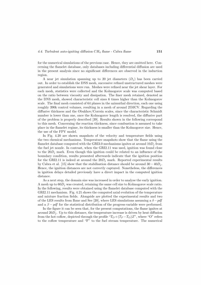
4.4. Turbulent auto-igniting diffusion CH4 flame - Cabra flame 151
for the numerical simulations of the previous case. Hence, they are omitted here. Con-cerning the flamelet database, only databases including differential diffusion are usedin the present analysis since no significant differences are observed in the inductionregion.
A near jet simulation spanning up to 20 jet diameters (Dj) has been carriedout. In order to establish the DNS mesh, successive refined unstructured meshes weregenerated and simulations were run. Meshes were refined near the jet shear layer. Foreach mesh, statistics were collected and the Kolmogorov scale was computed basedon the ratio between viscosity and dissipation. The finer mesh retained, denoted asthe DNS mesh, showed characteristic cell sizes 6 times higher than the Kolmogorovscale. The final mesh consisted of 64 planes in the azimuthal direction, each one usingroughly 390k control volumes, resulting in a mesh of around 25MCV. Regarding thediffusive thickness and the Obukhov/Corrsin scales, since the characteristic Schmidtnumber is lower than one, once the Kolmogorov length is resolved, the diffusive partof the problem is properly described [39]. Results shown in the following correspondto this mesh. Concerning the reaction thickness, since combustion is assumed to takeplace in the flamelet regime, its thickness is smaller than the Kolmogorov size. Hence,the use of the FPV model.
In Fig. 4.20 are shown snapshots of the velocity and temperature fields usingthe two chemical mechanisms. Temperature snapshots show that the flame using theflamelet database computed with the GRI3.0 mechanisms ignites at around 10Dj fromthe fuel jet nozzle. In contrast, when the GRI2.11 was used, ignition was found closeto the 20Dj mark. Even though this ignition could be related to an influence of theboundary condition, results presented afterwards indicate that the ignition positionfor the GRI2.11 is indeed at around the 20Dj mark. Reported experimental resultsby Cabra et al. [15] show that the stabilisation distance should be around 30− 40Dj .Hence, the ignition distances are not correctly captured. Nonetheless, the differencesin ignition delays detailed previously have a direct impact in the computed ignitiondistance.
As a next step, the domain size was increased in order to analyse the early ignition.A mesh up to 60Dj was created, retaining the same cell size to Kolmogorov scale ratio.In the following, results were obtained using the flamelet database computed with theGRI2.11 mechanism. Fig. 4.21 shows the computed axial evolution of the temperatureand mixture fraction fields. Alongside are plotted the experimental results and twoof the LES results from Ihme and See [20], where LES simulations assuming a δ−pdfand a β − pdf for the statistical distribution of the progress-variable were performed.
In the figure it can be seen that, for the present computations, the flame ignites ataround 20Dj . Up to this distance, the temperature increase is driven by heat diffusionfrom the hot coflow, depicted through the profile “TO+(TF−TO)Z”, where “O” refersto the coflow temperature and “F” to the fuel stream temperature. The numerical

152Chapter 4. Differential diffusion effects in the progress-variable definition for
Flamelet/Progress-variable models for non-premixed flames
(a) GRI3.0
(b) GRI2.11
Figure 4.20: Instantaneous snapshots of the near jet DNS simulation using theGRI3.0 and GRI2.11 detailed mechanism. The upper side of each picture shows thetemperature field in [K]. The lower side presents the velocity field in [m/s]. Axialand radial distances have been made non-dimensional using the fuel jet diameterDj .

4.4. Turbulent auto-igniting diffusion CH4 flame - Cabra flame 153
0
500
1000
1500
2000
2500
0 15 30 45 60 75
T[K]
y/D
Exp.Present workTO + (TF-TO)Z
0
200
400
600
0 15 30 45 60 75
Trms[K]
y/D
Ihme & See(2010) Cv δ-pdfIhme & See(2010) Cv β-pdf
0.2
0.4
0.6
0.8
1
0 15 30 45 60 75
Z
y/D
0
0.04
0.08
0.12
0 15 30 45 60 75
Zrms
y/D
Figure 4.21: Axial profiles of temperature (top) and mixture fraction (bottom).Experimental results from Cabra et al.[15] and LES results from hme and See [20]are also plotted. For the latter, two profiles are plotted corresponding to resultsobtained using different pdf for the progress-variable variance Cv.
simulation shows excellent agreement up to that point. Beyond, heat released fromcombustion enters into play and increases the temperature further. Compared toprevious LES results, the present results show a similar trend to those obtained whena δ−pdf was assumed for the progress-variable variance. Results from Domingo et al.[9] also showed a dependence on the modelling of the progress-variable variance. Thiscould indicate that the FPV model sets one flamelet in each control volume, whereinstead there should be more. However, no significant differences were observed whenresults from the present mesh were compared to previous results using a coarser mesh.
The experimental measurements of the velocity of Gordon [38] indicate that thefuel jet is self-similar. In Fig. 4.22, normalised velocity profiles at different axiallocations are shown together with a mean normalised experimental profile. Goodagreement is observed between numerical computations and experimental measure-ments.
In the UFPV model an important parameter is the stoichiometric scalar dissipationrate, which characterises the strain applied to the flamelet. In addition, the progress-variable acts as a tracker of the evolution of the chemical reaction, which can be relatedto a flamelet time-scale. Fig. 4.23 shows the axial evolution of these two quantitiescompared against LES results from Ihme and See [20]. It can be observed thatthe temporally and azimuthally averaged scalar dissipation rate conditioned on thestoichiometric mixture fraction is higher than the LES one. Regarding the lagrangian

154Chapter 4. Differential diffusion effects in the progress-variable definition for
Flamelet/Progress-variable models for non-premixed flames
0
0.2
0.4
0.6
0.8
1
1.2
0 0.5 1 1.5 2 2.5 3
(V - Vcoflow)/VO
r/r1/2
y/D=15y/D=20y/D=30y/D=40
Exp. mean
Figure 4.22: Normalised radial velocity profiles. Velocity is normalised usingthe excess velocity at the centreline VO = V (r = 0) − Vcoflow and the radialposition is normalised using the half radius r1/2, defined as the radial positionwhere (Vr − Vcoflow) = VO/2.
flamelet time, it is computed as
τ(y) =
∫ y
0
1
〈Vst(ζ)〉dζ (4.21)
where 〈Vst〉 = 〈V |Z = Zst〉 is the axial velocity conditioned on the stoichiometricmixture fraction. Present computations show a marked increase in its value whichimplies that at the stoichiometric mixture fraction surface the axial velocities arelower. Hence, flow residence times are higher in the present computations, whichcould account in part for the shorter ignition distance.
In Fig. 4.23b is also shown the evolution of the temperature conditioned on thestoichiometric mixture fraction. It can clearly be seen the transient evolution of theflamelets in composition space. Previously, when a suitable definition for the progress-variable was sought, it was stated that there were overlapping regions at low χst closeto the stable branch. Taking into account the axial evolution shown in the figure, itcan be seen that the influence of this non-bijective regions is limited.
4.5 Conclusions
The definition of the progress-variable has been shown to be sensitive to the caseconsidered as well as the diffusion mode. Common definitions have been considered,and it has been argued the convenience of increasing the number of considered speciesand/or the use of unequal weights among the species used to define the progress-variable. Minor species, which required large coefficients, have been shown to becapable of ensuring monotonically varying progress-variables. Improvements have

4.5. Conclusions 155
1e-05
0.0001
0.001
0.01
0.1
1
0 10 20 30 40 50 60 70 80 0
50
100
150
200
250
300
350
400
χst D/Vjet
τ Vjet/D
y/D
χstχst LES
τ
τ LES
(a) Non-dimensional axial evolution of sto-ichiometric scalar dissipation rate and la-grangian flamelet time
1000
1500
2000
2500
1 10 100 1000
Tst [K]
χst [s-1]
y/D=10
y/D=15
y/D=20
y/D=30
y/D=40y/D=50
S-shaped curve
(b) Axial evolution of the temperatureat Zst
Figure 4.23: Axial evolution of derived quantities. Results denoted by LES aretaken from Ihme and See [20].
been proposed for unsteady and radiation FPV model for two different flames, forcases using either Fickian or differential diffusion models. Lower success was hadfor the steady FPV. The presented alternatives were obtained manually and a moresystematic approach would lead to better definitions. An automated method, suchas the one presented by Ihme et al [10], could provide a suitable definition. Thepresented results provide an insight on the effect of different species in the progress-variable definition.
The definition of the progress-variable accounting for secondary equilibrium species,such as H2 and CO, may help in improving the monotonic growth at the stable branchof the S-shaped curve. However, at the unstable branch they may have the oppositeeffect, since the burned mixture is not close to its equilibrium values, specially at lowstoichiometric scalar dissipation rates. No fully monotonic definition has been foundfor the steady FPV model for the DLR FLame. CD2 has been argued to be betterfitted for the present case. The unsteady variant with the differential diffusion modelshowed overlapping regions near the stable burning solution at low and intermediateχst. These were the result of a narrower transient process compared to the Fickianone, which causes a build-up of reaction products. Regarding the FPV model withradiation, a complex evolution of the progress-variable has been found, which requiredadjusting several coefficients of the progress-variable definition in order to obtain bi-jective functions for both diffusion models. Different definitions were required foreach diffusion model. However, the reaction rates for these progress-variable defini-tions were not always positive. Overall, both diffusion model and combustion model,steady, unsteady or radiation, have a large impact on the progress-variable definitionto be used.

156 References
The stabilization mechanism for the DLR Flame A has been shown to be greatlydependent on the inclusion of differential diffusion effects, which increased the burningregion in the flamelet space compared to the Fickian one: increased stable tempera-tures, increased extinction scalar dissipation rate and reduced ignition temperatures.
Regarding the self-igniting case, namely the Cabra Flame, an unsteady Flamelet/Progress-Variable has been used to model it. Prior to the numerical simulationsin physical space, the flamelet database has been analysed considering the effectsof chemical mechanism and differential diffusion. It has been shown that of thetwo chemical mechanisms studied, the GRI3.0 shows a shorter ignition delay whencomputing flamelet solutions compared to the GRI2.11. Afterwards, it has beenshown that this shorter ignition delay manifests in a shorter ignition distance whennumerical simulations were carried out in physical space. Concerning the definitionof the progress-variable, it has been shown that differential diffusion is in generalnot a critical issue. However, during the induction phase, significant differences areobserved. In order to account for this different path, a new definition of the progress-variable is proposed. This new definition is mostly monotonic. However, at low χstthere remain non-monotonic regions, which are shown to have a limited effect on thesimulations since ignition takes place close to χi.
Concerning the DNS simulations, a deviation from the reported experimental ob-servations is observed. The flame ignites at shorter distances. However, good agree-ment in the non-reacting zones is observed. Since the flame ignites too early, nu-merical profiles deviate from the experimental ones at higher axial distances. It hasbeen shown that the present results show a similar trend as the LES results fromIhme and See [20] when a δ − pdf was used, which could indicate that the flameletdatabase is representing different states through one single flamelet. Concerning de-rived quantities, and specifically the stoichiometric scalar dissipation rate, a similartrend was observed compared to reported results from LES simulations. However, thelagrangian flamelet time showed higher values compared to LES results, indicatinglower velocities at the stoichiometric mixture fraction surface. Similarly, as reportedfrom experiments, the computed velocity profiles show that the flame is self similar.
References
[1] T. Poinsot and D. Veynante. Theoretical and Numerical Combustion. R.T.Edwards Inc., 2005.
[2] N. Peters. Turbulent Combustion. Cambridge University Press, 2000.
[3] H. Pitsch and N. Peters. A consistent flamelet formulation for non-premixed com-bustion considering differential diffusion effects. Combustion and Flame, 114:26–40, 1998.

References 157
[4] C.D Pierce and P. Moin. Progress-variable approach for large-eddy simulationof non-premixed turbulent combustion. Journal of Fluid Mechanics, 504:73–97,2004.
[5] H. Pitsch and M. Ihme. An unsteady flamelet/progress variable method forles of nonpremixed turbulent combustion. In Proceedings of the 43rd AerospaceSciences Meeting and Exhibit, 2005.
[6] M. Ihme, C.M. Cha, and H. Pitsch. Prediction of local extinction and re-ignitioneffects in non-premixed turbulent combustion using a flamelet/progress variableapproach. Combustion and Flame, 30(1):793–800, 2005.
[7] M. Ihme and H. Pitsch. Prediction of extinction and reignition in nonpremixedturbulent flames using a flamelet/progress variable model 2. Application in LESof Sandia flames D and E. Combustion and Flame, 155(1-2):90–107, 2008.
[8] a. W. Vreman, J. a. Oijen, L. P. H. Goey, and R. J. M. Bastiaans. Subgridscale modeling in large-eddy simulation of turbulent combustion using premixedflamelet chemistry. Flow, Turbulence and combustion, 82(4):511–535, 2008.
[9] P. Domingo, L. Vervisch, and D. Veynante. Large-eddy simulation of a liftedmethane jet flame in a vitiated coflow. Combustion and Flame, 152(3):415–432,2008.
[10] M. Ihme, L. Shunn, and J. Zhang. Regularization of reaction progress variablefor application to flamelet-based combustion models. Journal of ComputationalPhysics, 231(23):7715–7721, 2012.
[11] R. Hilbert, F. Tap, H. El-Rabii, and D. Thevenin. Impact of detailed chemistryand transport models on turbulent combustion simulations. Progress in Energyand Combustion Science, 30:61–117, 2004.
[12] K. W. Lee and D. H. Choi. Prediction of NO in turbulent diffusion flames usingeulerian particle flamelet model. Combustion Theory And Modelling, 12(5):905–927, 2008.
[13] W. Meier, R.S. Barlow, Y.-L. Chen, and J.-Y. Chen. Raman/Rayleigh/LIFmeasurements in a turbulent CH4/H2/N2 jet diffusion flame: Experimental tech-niques and turbulence-chemistry interaction. Combustion and Flame, 123:326–343, 2000.
[14] V. Bergmann, W. Meier, D. Wolff, and W. Stricker. Application of spontaneousRaman and Rayleigh scattering and 2D LIF for the characterization of a tur-bulent CH4/H2/N2 jet diffusion flame. Applied Physics B-Lasers And Optics,66:489–502, 1998.

158 References
[15] R. Cabra, J. Chen, R. Dibble, A. Karpetis, and R Barlow. Lifted methane–airjet flames in a vitiated coflow. Combustion and Flame, 143(4):491–506, 2005.
[16] D. Carbonell. Numerical studies of diffusion flames. Special emphasis on flameletconcept and soot formation. PhD thesis, Polytechnic University of Catalonia,Terrassa, Spain, 2010.
[17] J.S. Kim and F.A. Williams. Structures of flow and mixture-fraction fields forcounterflow diffusion flames with small stoichiometric mixture fractions. SIAMJournal On Applied Mathematics, 53:1551–1566, 1993.
[18] H. Pitsch, M. Chen, and N. Peters. Unsteady flamelet modeling of turbulenthydrogen-air diffusion flames. Twenty-Seventh Symposium (International) onCombustion, pages 1057–1064, 1998.
[19] H. Pitsch. Improved pollutant predictions in large-eddy simulations of turbu-lent non-premixed combustion by considering scalar dissipation rate fluctuations.Proceedings of the Combustion Institute, 29:1971–1978, 2002.
[20] M. Ihme and Y.C. See. Prediction of autoignition in a lifted methane/air flameusing an unsteady flamelet/progress variable model. Combustion and Flame,157(10):1850–1862, 2010.
[21] H. Pitsch. Modeling of radiation and nitric oxide formation in turbulent non-premixed flames using a flamelet/progress variable formulation. Physics of Flu-ids, 20(5):055110, 2008.
[22] R.S. Barlow, J.H. Karpetis A.N., Frank, and J.-Y. Chen. Scalar profiles andNO formation in laminar opposed-flow partially premixed methane/air flames.Combustion and Flame, 127(3):2102–2118, 2001.
[23] J. a. van Oijen and L. P. H. de Goey. Modelling of premixed counterflow flamesusing the flamelet-generated manifold method. Combustion Theory And Mod-elling, 6(3):463–478, 2002.
[24] E. Giacomazzi, F.R. Picchia, and N. Arcidiacono. A review of chemical diffusion:Criticism and limits of simplified methods for diffusion coefficient calculation.Combustion Theory And Modelling, 12:135–158, 2008.
[25] O. Lehmkuhl, C.D. Perez Segarra, R. Borrell, M. Soria, and A. Oliva. Ter-mofluids: A new parallel unstructured CFD code for the simulation of turbulentindustrial problems on low cost PC cluster. Proceedings of the Parallel CFDConference, pages 1–8, 2007.

References 159
[26] L.F. Shampine, B.P. Sommeijer, and J.G. Verwer. IRKC: An IMEX solver for stiffdiffusion-reaction PDE’s. Journal of Computational and Applied Mathematics,196:485–497, 2006.
[27] W.L. Grosshandler. RADCAL: A narrow-band model for radiation calculationsin a combustion environment. Technical Note 1402, NIST, 1993.
[28] R.W.C.P. Verstappen and A.E.P. Veldman. Symmetry-preserving discretizationof turbulent flow. Journal of Computational Physics, 187:343–368, 2003.
[29] M. S. Darwish and F. H. Moukalled. Normalized variable and space formulationmethodology for high-resolution schemes. Numerical Heat Transfer, Part B:Fundamentals, 26:76–96, 1994.
[30] H. Pitsch. Unsteady flamelet modelling of differential diffusion in turbulent jetdiffusion flames. Combustion and Flame, 123:358–374, 2000.
[31] F. Nicoud and F. Ducros. Subgrid-scale stress modeling based on the squareof the velocity gradient tensor. Flow, Turbulence and combustion, 62:183–200,1999.
[32] C.D. Pierce and P. Moin. A dynamic model for subgrid-scale variance and dissi-pation rate of a conserved scalar. Physics of Fluids, 10:3041, 1998.
[33] M. Ihme and H. Pitsch. Modeling of radiation and nitric oxide formation inturbulent nonpremixed flames using a flamelet/progress variable formulation.Numerical Heat Transfer, Part B: Fundamentals, 26:76–96, 1994.
[34] W. L. Chan, H. Kolla, J. H. Chen, and M. Ihme. Assessment of model as-sumptions and budget terms of the unsteady flamelet equations for a turbulentreacting jet-in-cross-flow. Combustion and Flame, 161(10):2601–2613, 2014.
[35] J. Michel, O. Colin, C. Angelberger, and D. Veynante. Using the tabulated dif-fusion flamelet model adf-pcm to simulate a lifted methane–air jet flame. Com-bustion and Flame, 156(7):1318–1331, 2009.
[36] M. Ihme and H. Pitsch. Prediction of extinction and reignition in nonpremixedturbulent flames using a flamelet/progress variable model 1. A priori study andpresumed PDF closure. Combustion and Flame, 155(1-2):70–89, 2008.
[37] E. Knudsen, E.S. Richardson, E.M. Doran, N. Pitsch, and J.H. Chen. Modelingscalar dissipation and scalar variance in large eddy simulation: Algebraic andtransport equation closures. Physics of Fluids, 24:055103, 2012.

160 References
[38] R.L. Gordon. A numerical and experimental investigation of autoignition. PhDthesis, University of Sidney, 2008.
[39] L. Vervisch and P. Poinsot. Direct numerical simulation of non-premixed turbu-lent flames. Annual Review of Fluid Mechanics, 30:655–691, 1998.

5
Large Eddy Simulation of ashear stabilised turbulentdiffusion flame using aFlamelet/Progress-Variablemodel.
Main contents of this chapter have been presented at international conferences::J. Ventosa, O. Lehmkuhl, C.D. Perez-Segarra, J. Muela, A. Oliva. Comparative study of
subfilter scalar dissipation rate and mixture fraction variance models. In Proceedings of the11th World Congress on Computational Mechanics (WCCM XI); 5th European Conferenceon Computational Mechanics (ECCM V); 6th European Conference on Computational FluidDynamics (ECFD VI) pp.5239 - 5248. Barcelona, Spain, July 2014.
J. Ventosa, O. Lehmkuhl, C.D. Perez-Segarra, A. Oliva. Assessment of subfilter scalardissipation rate and mixture fraction variance models . In Proceedings of the iTi Conference2014, Bertinoro, Italy, September 2014.
Abstract. A common approach to simulate diffusion flames with Large Eddy Simula-
tion (LES) models is to use a flamelet approach coupled with a probability density function
assumption, which require the characterisation of mixing at length scales shorter than the
mesh, which is described by the mixture fraction variance Zv and subgrid scalar dissipa-
tion rate χsgs. Four different models for evaluating them are assessed in the context of a
Flamelet/Progress-Variable (FPV) model. First, the Local Equilibrium model. Second, a
model using a transport equation for the variance. Lastly, two models using the variance
statistical definition Zv = Z2− Z2, together with either a transport equation for the squared
mixture fraction Z2 or a transport equation for the filtered squared mixture fraction gra-
dient |∇Z|2. The effect of the different models is assessed using a flame stabilised within
a shear layer. A simple turbulent jet CH4/H2/N2 diffusion flame is used due to its simple
flow and geometry configuration. Additionally, it is evidenced that correct characterisation
of subgrid mixing is critical in the description of the stabilisation mechanism. It is shown
161

162Chapter 5. Large Eddy Simulation of a shear stabilised turbulent diffusion flame
using a Flamelet/Progress-Variable model
that the model using a transport equation for the variance and the model using the variance
definition are not equivalent at the discrete level, even though they are equal at the contin-
uous level. Furthermore, the effect of the FPV model variant, steady, unsteady or radiation,
results in a different interaction with the mixing model. The subgrid mixing model is shown
to be critical for steady and unsteady models. The radiation model, which only contains a
subset of the flamelet space, overshadows the effect of subgrid mixing.

5.1. Introduction 163
5.1 Introduction
In non-premixed combustion, the flamelet regime has been widely studied since itis found in many technological designs. It is characterised by chemical reactions takingplace in thin laminar layers embedded within turbulent flow structures[1]. Therefore,the smallest eddies do not penetrate the reaction layer of the flame. Hence, through anappropriate coordinate transformation to a mixture fraction space [1] the combustionprocess may be split into a transport process and a diffusion-chemistry process. Theformer requires solving the Navier-Stokes equations, and the latter process reduces toa set of diffusion-reaction equations in mixture fraction space, where there appearsthe scalar dissipation rate. The latter introduces flow effects from physical space intothe flamelet equations.
The mixing process in diffusion flames is usually modelled through a passive scalar,the mixture fraction Z. In turbulent flows, due to the large span of spatial scalesinvolved, models are introduced to reduce the computational effort required. BothReynolds Averaged Navier-Stokes (RANS) and Large Eddy Simulation (LES) modelssplit the phenomenon of interest into a resolved and an unresolved part. Particularly,in LES the splitting is performed by means of a spatial filtering. A usual approachis to use the computational mesh as filter. Therefore, in LES the resolved mixturefraction describes mixing at the filter or grid level, and mixing at the subfilter levelis characterised by two interconnected quantities, the mixture fraction variance Zvand the subgrid scalar dissipation rate χsgs. The resolved mixture fraction is readilyavailable as solution of a transport equation. However both Zv and χsgs requiremodelling.
Solutions of the diffusion-reaction flamelet equations are laminar quantities andare parametrised as a function of laminar variables. Since the focus is on flames inturbulent flows, solution variables of the flamelet equations must be restated intoFavre averaged quantities. As turbulent quantities, they can be represented usingstatistical distributions, particularly through probability density functions (pdf ). Onthe one hand, transported probability density function methods were proposed inorder to compute these pdf [2]. However, with large chemical mechanisms and inconjunction with LES, the method becomes expensive. Furthermore, the diffusionprocess becomes an unclosed term and has to be modelled. On the other hand, modelsusing presumed pdf have been used successfully in many applications, even thoughthe statistical distribution of a given parameter had to be assumed beforehand.
Flamelet models used to simulate turbulent flames commonly rely on the β−pdf todescribe turbulence-chemistry interactions at the subfilter level. This pdf is definedas a function of the first moment, the mean, and the second central moment, thevariance. Consequently, mixing at the subgrid level is characterised by the mixturefraction variance. A further quantity of interest which appears in the modelling ofthe mixture fraction variance is the subgrid scalar dissipation rate.

164Chapter 5. Large Eddy Simulation of a shear stabilised turbulent diffusion flame
using a Flamelet/Progress-Variable model
The evaluation of the subgrid mixture fraction variance and the subfilter scalardissipation rate is a critical issue in combustion models using a presumed pdf ap-proach, such as Flamelet models and Conditional Moment Closure (CMC) models.In premixed flames with Presumed Conditional Moment (PCM) models, the varianceof the progress-variable represents a similar challenge. Both parameters model scalarmixing at the subgrid level, which in turn controls the combustion process. There-fore, accurate description of the subgrid mixing is critical as the Reynolds numberis increased. The first proposed models to evaluate both quantities were based ona local equilibrium hypothesis, where production and destruction of variance at thesubfilter level were assumed to cancel out. The proposed scale similarity model for themixture fraction variance [3], although being computationally efficient, was found toproduce erroneous estimations of the scalar mixing in technically relevant flow config-urations [4], thus being not suitable in many cases of industrial interest. In the past,several models have been proposed to account for deviations from local equilibrium.One option in order to take into account non-equilibrium effects is to construct atransport equation for the variance itself (VTE). Alternatively, being the variance an
statistical quantity, it can be computed through its definition, Zv = Z2− Z2. In turn,
this requires the computation of the second moment of the mixture fraction, Z2. Atransport equation is then usually employed (STE). Nonetheless, in both cases closurefor the subfilter dissipation rate is required. Algebraic expressions relating the sub-grid variance with the subfilter dissipation through a turbulent time-scale have beenproposed [4, 5]. Alternatively, closure for the scalar dissipation rate can also be per-formed solving a transport equation for the filtered squared gradient of the mixturefraction [6]. Each approach involves different equations using different closures. Fur-thermore, these two quantities, subgrid variance and subgrid scalar dissipation rate,are parameters of the flamelet database. Thus, differences in their predictions willimply different retrieved values from the flamelet database, and will lead to differentflame dynamics.
In the present work the DLR simple-jet [7, 8] is selected as study case because itsstabilisation mechanism is through the shear layer between fuel and oxidiser coflowstreams. Hence, mixing is a critical aspect to be modelled. Other stabilisation mech-anisms for turbulent flows at high Reynolds numbers are the use of pilot flames,recirculation and bluff-bodies, among others. However, since the focus of the presentstudy is the modelling of subgrid mixing these other mechanisms overshadow the roleof mixing.
The DLR simple-jet features a fuel jet sorrounded by a coflowing stream of oxidiser.The fuel is a mixture of CH4 and H2 diluted in N2. Hydrogen was added to the fuelin order to increase the burning rate and aid in the stabilisation [7]. Experimentallythis flame is attached to the fuel nozzle rim. The stabilisation mechanism for thisflame is then mostly due to diffusion through the shear layer between the two reactant

5.1. Introduction 165
streams. The case will serve to analyse the effect of several subgrid models on theflame predictions.
Due to its canonical geometry and configuration, this flame has been extensivelyused to validate several combustion models. Pitsch [9] used the classical unsteadyflamelet model to study differential diffusion effects in this flame. Emami and Eshgh-inejad Fard [10] used this flame to study a flamelet approach with Artificial NeuralNetworks. Lindsted and Ozarovsky [11] used a pdf model, Vogiatzaki [12] applieda Multiple Mapping Conditioning (MMC) model and Wang and Pope [13] tested aLES/pdf model coupled with a Flamelet/Progress-variable (FPV) model. Fairweatherand Woolley [14] used a first order CMC model to study several chemical mechanisms.Lee and Choi [15, 16] used an Eulerian Particle Flamelet model (EPFM) to study NOemissions. Ihme et al. [17, 18] performed a LES simulation using a Flamelet/Progress-Variable (FPV) model to study combustion generated noise.
Most of the aforementioned studies were conducted using Reynolds AveragedNavier-Stokes (RANS) models, where the turbulent viscosity is usually higher thanthe molecular one, or with PDF methods, where mixing itself requires closure. In LESthis is not the case, where molecular transport can play a significant role as turbulentand molecular diffusivities can be of the same order. Furthermore, in combustionphenomena molecular transport is enhanced due to the exothermicity of chemical re-actions [19]. Both Wang and Pope [13] and Ihme et al. [17] reported LES simulationsusing a FPV model, where a single flamelet was used in the former and only thesteady burning solutions were included in the latter [18].
The aim of this chapter is to evaluate several subgrid mixing models in the contextof a diffusion flame. Three variants of the Flamelet/Progress-Variable model are used:steady, unsteady and including radiation. The described models for subgrid varianceand subgrid scalar dissipation rate are used and their effect in predicted profiles andflame stabilisation compared. Thus, the study focuses on different implementationsof the subgrid mixing closure and their effect on the flame predictions. It is shownthat incorrect capture of subgrid mixing results in flame lift-off, even though exper-imentally an attached flame was reported. Furthermore, the thermal effects of theflame on the shear layer are discussed.
The chapter is organized as follows: first, the mathematical formulation for theLES model, the combustion model and subgrid closures are presented. The experi-mental case and computational domain are then described. Afterwards, results usingthe different FPV variants and subgrid closures are presented.

166Chapter 5. Large Eddy Simulation of a shear stabilised turbulent diffusion flame
using a Flamelet/Progress-Variable model
5.2 Mathematical model
5.2.1 LES model
Large Eddy Simulation describes the motion of the large scales of the flow, whereasthe small scales are modelled. Scale splitting is performed by means of a low-passfilter,
ρφ =
∫Ω
ρφG(x, ξ)dξ (5.1)
In grid based, implicit filtering the filter kernel G(x, ξ) becomes a top-hat filter withsize ∆ = (hi)
1/3, where hi is the mesh spacing in the i -direction. Additionally,for variable density flows, the filtered quantities are density weighted, or Favre fil-tered. Favre filtered quantities can be related to Reynolds filtered quantities throughρφ = ρφ. Therefore, applying the filtering operation to the low-Mach Navier-stokesequations, the equation of mass and momentum conservation become
∂ρ
∂t+∂ρuj∂xj
= 0 (5.2)
∂ρui∂t
+∂ρuj ui∂xj
= − ∂p
∂xi+
∂
∂xj
((µ+ µt)σij
)+ ρgi (5.3)
where ρ, p and ui represent the filtered density, the filtered dynamic pressure and theFavre filtered velocity, respectively. The diffusive fluxes, including the rate of strain
and the deviatoric part, are σij =
(∂ui∂xj
+∂uj∂xi− 2
3δij∂uk∂xk
). Turbulent subgrid fluxes
have been modelled through an eddy-diffusivity assumption, where the turbulentsubgrid viscosity µt is closed by means of the Wall-Adapting Local Eddy diffusivity(WALE) model [20] in the context of a Variational Multiscale Model [21]. The choiceof subgrid turbulence model is discussed along with the model for the subgrid scalarturbulent diffusivity in Sec. 5.4.1.
Thermochemical properties, such as the density and molecular diffusivities, areprovided by the combustion model, and are discussed in the following.
5.2.2 Flamelet/Progress-Variable (FPV) model
In the flamelet regime, chemically active layers are thinner than the size of theKolmogorov scale. Therefore, it is justified to assume that turbulent eddies do notpenetrate the reaction zone. Thus, the flame can be considered to exist in a quasi-laminar flow field within those eddies [1]. Consequently, the flame can be consideredas an ensemble of laminar flames surrounded by turbulent structures, capable only ofwrinkling and straining the flame.
Hence, defining a new coordinate system described by the mixture fraction andapplying a coordinate transformation to the species and energy equations, as describedby Pitsch and Peters [22], the flamelet equations are obtained

5.2. Mathematical model 167
ρ∂φ
∂t= ρ
χZ2
∂2φ
∂Z2+ Sφ (5.4)
where φ denotes species mass fractions and temperature, Sφ includes the equation’s
source term and other additional terms and χZ = 2Dz
(∂Z∂xi
∂Z∂xi
)is the scalar dissi-
pation rate. The latter introduces flow effects from the transport process into thediffusion-chemistry process.
The scalar dissipation rate dependence on the mixture fraction distribution inphysical space precludes solving the flamelet equations in a preprocessing stage.Nonetheless, through an analogy between diffusion flames in the flamelet regime andcounterflow flames [1], the scalar dissipation rate can be described through an ana-lytical expression in mixture fraction space
χZ(Z) = χstf(Z)
f(Zst)(5.5)
f(Z) = exp(−2[erfc−1(2Z)]2) (5.6)
where erfc−1 is the inverse of the complementary error function. Furthermore, thisexpression was also derived from the analysis of unsteady mixing layers [1].
Flamelet modelling of diffusion flames offers a dimensionality reduction by map-ping the multicomponent diffusion-reaction process, the flame problem, into a limitedset of transported scalars. Solutions of one-dimensional flamelets in their steady stateform can be expressed as a state relation
φ = ξφ(Z, χst) (5.7)
where χst is the scalar dissipation rate at the stoichiometric mixture fraction. Plottingthe stoichiometric temperature as a function of the stoichiometric scalar dissipationrate the S-shaped curve is obtained, Fig.5.1.
The upper branch of this curve represents the stable burning state, the middleone the unstable burning solution and the lower one the extinguished state or puremixing. The turning point between the upper and lower branch corresponds to thequenching scalar dissipation χq. Although with Eq. (5.4) all solutions of the S-shapedcurve can be obtained by setting Z and χst, Eq. (5.7) does not offer a unique rep-resentation of the curve. Hence, only one branch can be represented. Applicationsof the flamelet model typically represents only the stable burning branch and thestable non-burning solution for χst > χq. This shortcoming of flamelet models canbe overcome introducing a new flamelet parameter Λ = c|Zst, as proposed by Pierceand Moin [23], where the progress-variable c is usually defined as the summation of

168Chapter 5. Large Eddy Simulation of a shear stabilised turbulent diffusion flame
using a Flamelet/Progress-Variable model
0
400
800
1200
1600
2000
2400
0.1 1 10 100 1000
Tst [K]
χst [s-1]
Stable BranchUnstable Branch
Radiation subspaceRadiation Stable Solution
Mixing line
Figure 5.1: S-shaped curve for the DLR Flame. Dotted region represents theradiation accessible flamelet subspace.
several species mass fractions. Using this parameter the full S-shape curve can beuniquely represented by a state relation
φ = ζφ(Z,Λ) (5.8)
Therefore, the FPV combustion model uses a unique set of parameters to representall possible flame states, defined by a mixture fraction Z and a flamelet parameterΛ. Therefore, once Z and Λ are computed, Eq. (5.8) can be used to retrieve anyflamelet solution. It is possible to solve a transport equation for Λ. However, it ismore convenient to solve a transport equation for the progress-variable itself, becausein turbulent flames the transport equation for Λ contains several terms which aredifficult to model. Since the progress-variable can be recovered using the state relationEq. 5.8, the flamelet parameter Λ can be expressed as a function of the progress-variable, Λ = ζ−1
c (Z, c). This implies that there exists a bijective relation betweenthe progress-variable and the progress-variable parameter. Introducing it in Eq. 5.8,a state relation can be defined relating the flamelet scalars to Z and c (for steadycases)
φ = zφ(Z, c) (5.9)
For LES simulations, this state relation must be recast for Favre-filtered quantities.

5.2. Mathematical model 169
Then, turbulent quantities are expressed through statistical distributions
φ =
∫ ∫ζφ(Z,Λ)P (Z,Λ)dZdΛ (5.10)
where P (Z,Λ) denotes the Favre joint pdf of Z and Λ. Assuming that the flameletparameter Λ is statistically independent with respect to the mixture fraction Z, thenthe joint pdf is reduced to its marginal pdf, P (Z,Λ) = P (Z)P (Λ). The marginal pdfof the mixture fraction is modelled using a β-pdf [24]. Additionally, the marginal pdfof Λ is assumed to be described by a δ-pdf function [23, 25]. Therefore,
P (Z,Λ) = β(Z; Z, Zv)δ(Λ− Λ∗) (5.11)
The β − pdf introduces the mixture fraction variance Zv as a parameter of the staterelation.
With the definition of the pdf to model turbulent effects on the laminar flameletlibrary, a turbulent flamelet library can be constructed. Recasting the turbulentflamelet library as performed previously for the laminar case, all thermochemicalvariables from the steady state solution of the flamelet equations can be stated as afunction of three parameters, Z, c and Zv
φ = ζφ(Z, Zv, Λ)→ φ = zφ(Z, Zv, c) (5.12)
In order to retrieve the data from the database, the Favre filtered mixture fraction Z,its subfilter variance Zv and progress variable c are computed in physical space. Bothmixture fraction and progress-variable are transported quantities in physical space
ρ∂Z
∂t+ ρuj
∂Z
∂xj=
∂
∂xj
(ρ(DZ +DZ,t
) ∂Z∂xj
)(5.13)
ρ∂c
∂t+ ρuj
∂c
∂xj=
∂
∂xj
(ρ(Dc +Dc,t
) ∂c∂xj
)+ ˜wc (5.14)
where DZ and Dc are the mixture fraction and progress-variable molecular diffusivi-ties, respectively. Analogously, DZ,t and Dc,t are the turbulent diffusivities, which arecomputed using a constant Schmidt number Sct = 0.4. The progress-variable reactionrate ˜wc is defined as the summation of the reaction rates of the species defining theprogress-variable. The mixture fraction variance is not readily available and requiresmodelling. Several closures are discussed in the following section.
Extensions of the steady FPV model have been published to include either thetransient term of the flamelet equations or to account for heat losses due to radiation.On the one hand, Pitsch and Ihme [25] introduced χst as an additional parameter to

170Chapter 5. Large Eddy Simulation of a shear stabilised turbulent diffusion flame
using a Flamelet/Progress-Variable model
account for unsteady effects. On the other hand, Ihme and Pitsch [26] used the en-thalpy to account for radiation heat losses. Following a similar procedure as describedfor the steady database, solutions of the flamelets equations can be expressed as stateequations. The thermochemical database accessed during numerical simulations foreach variant reads
φ = zSFPVφ (Z, Zv, c) (5.15a)
φ = zUFPVφ (Z, Zv, c, χst) (5.15b)
φ = zRFPVφ (Z, Zv, c, h) (5.15c)
where φ represents the different variables retrieved from the flamelet database, suchas the density ρ, the progress-variable reaction rate ˜wc, the molecular mixture fractiondiffusivity DZ , etc.
The steady FPV (SFPV) model represents the curve defined by the stable burning,unstable burning and non-burning branches, depicted in Fig. 5.1. The unsteady FPV(UFPV) model is able to represent all states in the flamelet subspace, including steadysolutions and the transient solutions between them. For the radiation FPV (RFPV),the radiation subspace is depicted in the figure by the dotted region, which representsthe region where radiation effects are significant. The reader is referred to references[23, 25, 26] for details on the generation of the databases.
A last aspect to define is the form of the progress-variable. It is a tracking quantitywhich, together with the mixture fraction, must uniquely define the thermochemicalstate. It is usually defined as a linear summation, or in some cases a weighted summa-tion, of several species. In the present case, a linear combination of CO, CO2, H2 andH2O is used when steady FPV database is employed, c = YCO +YCO2 +YH2 +YH2O,as suggested by Ihme [17]. A slightly modified definition is taken when the unsteadyFPV database is used, c = YCO +YCO2
+YH2 +YH2O + 5YC2H2. The GRI 3.0 mecha-
nism [27] is used to generate the chemical database. Differential diffusion effects havebeen considered in the solution of the flamelet equations.
Subgrid ClosuresThe variance, or second central moment, which is required to retrieve solutions
from the FPV database, is defined in terms of a probability density function [28]
Zv = Z2 − Z2 (5.16)
where Zv denotes the subfilter mixture fraction variance. To compute it, there aretwo possibilities. Either a transport equation for the variance itself [28] is used (VTE)
ρ∂Zv∂t
+ ρu∂Zv∂xi
=∂
∂xi
(ρ(DZ +Dt,Z)
∂Zv∂xi
)+ 2ρ(DZ +Dt,Z)
∂Z
∂xi
∂Z
∂xi− ρχZ (5.17)

5.2. Mathematical model 171
or a transport equation for the second moment of the mixture fraction Z2 (STE) [6]
ρ∂Z2
∂t+ ρu
∂Z2
∂xi=
∂
∂xi
(ρ(DZ +Dt,Z)
∂Z2
∂xi
)− ρχZ (5.18)
A further parameter is here introduced to characterise the mixing state, the filteredscalar dissipation rate χZ . In both cases closure for the scalar dissipation rate isrequired
χZ = 2DZ∂Z
∂xi
∂Z
∂xi= 2DZ
∂Z
∂xi
∂Z
∂xi+ χZ,sgs (5.19)
where χZ,sgs = 2DZ
(∂Z∂xi
∂Z∂xi− ∂Z
∂xi∂Z∂xi
)is the subfilter dissipation rate.
Even though the VTE and STE models are equivalent at the continuous levelthrough Eq. (5.16), Kemenov et al. [29] and Kaul et al. [30] showed that they are notexactly equivalent at the discrete level. For example, the effect of the squared gradient
is opposite between the two models. In the STE model 2DZ∂Z∂xi
∂Z∂xi
is a dissipation
term and in the VTE model 2Dt,Z∂Z∂xi
∂Z∂xi
is a production term. Therefore, numericalerrors in the computation of the gradient or differences in the mixture fraction fieldwill have a different impact in each model.
In order to close the model for Zv, closure for χsgs is required. In Eq. (5.17), ifproduction and destruction of the mixture fraction variance at the small scales areassumed to be in equilibrium [3, 31], denoted as the Local Equilibrium Assumption(LEA), the scalar dissipation rate becomes
χZ = 2(DZ +Dt,Z)∂Z
∂xi
∂Z
∂xi(5.20)
However, with the LEA the mixture fraction variance requires a model as Eq. (5.17)with this assumption is just the transport equation of a passive scalar. Hence, a scalesimilarity model [3] for the mixture fraction variance may be used
ρZv = Cvar∆2ρ|∇Z| (5.21)
where Cvar is here calculated using the Leonard term Expansion Dynamic model(LED) [32]. Within the dynamic evaluation, a top-hat test filter with filter size∆ = 2∆ is used.
If non-equilibrium effects are to be considered, Eq. (5.20) cannot be used. Thus,alternative closures for the subfilter dissipation rate have to be used. Models usingeither an algebraic closure or a transport equation for the filtered gradient of themixture fraction have been proposed. On the one hand, the subgrid variance can be

172Chapter 5. Large Eddy Simulation of a shear stabilised turbulent diffusion flame
using a Flamelet/Progress-Variable model
related to the subfilter dissipation rate through a turbulent mixing time-scale [4, 5],the algebraic approach,
χZ,sgs =CZτZv = CZ
νt∆2
Zv (5.22)
1
τ=εsgsksgs
≈ νt∆2
(5.23)
where τ is a turbulent (mixing) time-scale, ksgs and εsgs are the subgrid turbulentkinetic energy and dissipation, respectively. The turbulent viscosity νt is used tomodel the latter. The model constant is of the form CZ = Cχ,Z(Cε/Cu), whereCχ,Z = 2 is a constant relating mechanical and scalar time-scales and (Cε/Cu) = 2 isrelated to the energy spectra [5]. Nevertheless, the effect of the constant is afterwardsinvestigated. In the context of RANS models, a similar functional relation betweenχsgs and Zv was proposed. The time-scale is related to the ratio of kinetic energyand kinetic energy dissipation and the constant takes a value of 2 [1].
On the other hand, closure for the scalar dissipation rate χZ can be achieved by
constructing a transport equation for the filtered squared gradient |∇Z|2 [6], heredenoted as SDR-TE. Evaluation of the SDR-TE requires modelling several unclosedterms and the evaluation of computationally expensive terms.
D
Dt
(ρ|∇Z|2
)=
∂
∂xi
(ρ(DZ +Dt,Z)
∂ |∇Z|2∂xi
)− 2ρ
(∂ui∂xj
∂Z
∂xi
∂Z
∂xj
)− 2ρDZ
(∂2Z
∂xi∂xj
)− 2
ρ
∂ρ
∂xi
∂Z
∂xi
(∂
∂xj
(ρDZ
∂Z
∂xj
))+ 2
∂ρDZ
∂xi
∂Z
∂xi
(∂2Z
∂x2j
)+ 2
∂Z
∂xi
∂Z
∂xj
(∂2ρDZ
∂xi∂xj
)+ Cprdρ
32νt∆2
(|∇Z|2 − |∇Z|2
)− 12Cvarρ
DZ
Zv
(|∇Z|2 − |∇Z|2
)2
(5.24)
where Cprd = 1 is a model constant and Cvar is dynamically evaluated using the LEDmodel, as performed for the equilibrium model Eq. (5.21).
Summarizing, the four closures used in the following are listed in Table 5.1

5.3. Turbulent diffusion CH4/H2/N2 flame - DLR A flame 173
Zv χsgsEquilibrium Model Eq. (5.21) Eq. (5.20)VTE Eq. (5.17) Eq. (5.22)STE Eq. (5.16), Eq. (5.18) Eq. (5.22)SDR-TE Eq. (5.16), Eq. (5.18) Eq. (5.24)
Table 5.1: List of subgrid mixing closures and the equations involved in eachmodel.
5.2.3 Numerical method
The set of equations for the conservation of mass Eq. (5.2), momentum (Eq. (5.3))and transport of the mixture fraction (Eq. (5.13)) and progress-variable (Eq. (5.14))are solved using a finite-volume approach. Particularly, 3D collocated meshes, ei-ther structured or unstructured. In order to preserve kinetic energy, a Symmetry-Preserving scheme [33] is used in the construction of the discrete convective term ofthe momentum equation. For the scalar convective terms, a SMART scheme is used[34]. A second order centred difference scheme is used to construct the discrete dif-fusive term for all transported quantities. Temporal integration is performed usinga linear multi-step method, as described in Chapter 2, with a second order Adams-Bashforth scheme in the predictor step and a Crank-Nicholson scheme in the correctorstep. The pressure-velocity coupling is solved through a Fractional Step method. ThePoisson equation is solved by means of FFT-based Poisson Solver by Borrell et al.[35], due to the use of an axysimmetric mesh with one circulating direction, as de-scribed in the next section.Numerical computations are performed using the general purpose unstructured andparallel object-oriented CFD code TermoFluids [36].
5.3 Turbulent diffusion CH4/H2/N2 flame - DLR A flame
The case of study is the axisymmetric jet flame denoted as DLR Flame A [7, 8],which was a standard flame used in the third “International Workshop on Measure-ment and Computation of Turbulent Nonpremixed Flames” (TNF Workshop) [37]. Itconsists of a D = 8mm wide fuel jet with a thinned rim at the exit. The inner fuel jetis composed of 33.2% H2, 22.1% CH4, and 44.7% N2 by volume and the outer jet isregular air with 20.1% O2. The fuel jet exit bulk velocity is fixed to Vb = 42.15m/s,resulting in a Reynolds number of Reb = 15, 200. The jet was mounted concen-trically to the coflow nozzle, which had a diameter of 140mm and provided air at0.3m/s. Both fuel and coflow air were at 300K. The stoichiometric mixture fractionis Zst = 0.167.

174Chapter 5. Large Eddy Simulation of a shear stabilised turbulent diffusion flame
using a Flamelet/Progress-Variable model
Regarding the computational mesh, two grids have been used, a fine and a coarseone. The former is a structured collocated mesh concentrated near the central jetwith 95x645x32 control volumes (CV) in the radial, axial and azimuthal directionsrespectively. Mesh sizes were compared against the Kolmogorov scale for this case,and ratios ranging between 15 and 20 were found in the regions of interest, thusensuring that the analysis was performed in the inertial range. The coarse meshwas an unstructured mesh which featured around 250 kCV, using 16 planes in theazimuthal direction. Unless otherwise stated, reported results correspond to the finermesh.
Inflow conditions for the fuel jet are taken from a fully developed turbulent pipeflow simulated in a preprocessing stage with Reb, Vb and D at the jet inflow temper-ature.
5.4 Results and discussion
The current flame, as reported experimentally, shows low levels of extinction andreignition and is attached to the flame nozzle rim indicating that the flame is rapidlyignited. Therefore, mainly the steady FPV is used. The unsteady and radiationvariants serve to assess the effect of the model choice on the subgrid quantities.
The flamelet database is discretised using 100x25x100 points for the mixture frac-tion, its variance and the progress-variable, respectively. For the unsteady variant 13different transient flamelets were considered. The radiation variant, due to computa-tional limitations, used 75x25x75x65 points in Z,Zv, c and h directions.
Differential diffusion effects are taken into account when building the flameletdatabase. For the present case, accounting for differential diffusion effects resultsin a significant increase in the extinction stoichiometric scalar dissipation rate χq, asshown in Chapter 4. Since no stabilisation mechanism is used, use of Fickian diffusionresults in the flame lifting-off and stabilising downstream of the fuel nozzle. Whenradiation heat losses are included, an Optically Thin Model (OTM) is used [38, 39].
5.4.1 Turbulent fluxes closure
First, the turbulent eddy diffusivity model used is assessed. Closures for theReynolds stress tensor have been extensively studied [40, 41] and new models are stillnowadays being postulated [20, 42]. Regarding the unresolved fluxes for the scalars,such as the temperature or the mixture fraction, usually a turbulent Prandtl, Schmidtor Lewis number is assumed. These non-dimensional numbers are either constantor dynamically computed in a similar way as the Dynamic Eddy Viscosity model(DEV) [41, 43]. Thus, there is wide range of closure combinations. Three differenteddy viscosity models for the Reynolds stress tensor are tested: The Dynamic EddyViscosity (DEV) [41], which is based on a strain invariant, the Wall-Adapting LocalEddy-viscosity (WALE) [20], which is based on strain and rotational invariants, and

5.4. Results and discussion 175
the QR [42], based on two strain invariants.When µt is computed using a Smagorinsky type eddy viscosity model with a dy-
namic evaluation of the scalar constant, originally developed for the energy equation,model consistency between momentum and scalars closures is ensured. Use of eddyviscosity models relying on different invariants, as in the WALE and QR models, re-sults in an inconsistency among models, leading to excessive diffusion, as shown inFig. 5.2, where the radial profiles of the mixture fraction and axial velocity at an axialdistance located at 5 nozzle diameters from the fuel jet nozzle (y/D = 5) are shown.Results were computed using the coarse mesh. On the one hand, the dynamic modelapplied to all variables (sgs4 ) shows the best agreement with the experimental data.On the other hand, combinations of the WALE or QR models with either a Schmidtnumber dynamically evaluated (sgs1, sgs6 ) or constant (sgs3, sgs7 ) showed higherdeviations at the curve tail. Both QR and WALE models coupled with a dynamicallyevaluated mixture fraction diffusivity show a widened profile. The dynamic model isnot applied to the progress-variable when the WALE is used because it was unstable.Either a constant Schmidt (sgs2 ) is used or the mixture fraction turbulent diffusivityis taken (Dc,t = DZ,t) (sgs1 ). We believe that the dynamic model applied to annon-conserved variable, namely the progress-variable, may be inadequate. If a con-stant turbulent Schmidt number is used, the WALE model shows a similar behaviouras the dynamic model applied to both the viscosity and diffusivity. Hence, modelconsistency appears to be important in order to properly evaluate turbulent fluxesand limit the effect of the diffusivity introduced by the turbulence model.
0
0.1
0.2
0.3
0.4
0.5
0.6
0.7
0.8
0.9
1
0 0.5 1 1.5 2 2.5
⟨Z~⟩
x/D
(a) Mixture fraction < Z >
0
10
20
30
40
50
60
0 0.5 1 1.5 2 2.5
⟨V~⟩ [m/s]
x/D
Experimental(sgs1) WALE µ - Dynamic Dt,Z = Dt,c
(sgs2) WALE µ - Dynamic Dt,Z - Sct Dt,c(sgs3) WALE µ - Sct Dt,Z , Dt,c
(sgs4) DEV µ - Dt,Z - Dt,c(sgs5) DEV µ - Dt,Z = Dt,c
(sgs6) QR µ - Dynamic Dt,Z = Dt,c(sgs7) QR µ - Sct Dt,Z , Dt,c
(b) Axial velocity < V >
Figure 5.2: Time-averaged distributions at y/D = 5 using different combinationsof subgrid closures for the unresolved turbulent fluxes. The equal sign in the key(= Dt,c) indicates that the progress-variable turbulent diffusivity is taken equal tothe corresponding one of the mixture fraction. Results correspond the coarse mesh.

176Chapter 5. Large Eddy Simulation of a shear stabilised turbulent diffusion flame
using a Flamelet/Progress-Variable model
Given the just described behaviour, the WALE model with a constant turbulentSchmidt number has been chosen in order to minimize the computational costs, sincethe WALE model does not require an explicit filtering operation.
5.4.2 Flame stabilisation
The first aspect to analyse is the stabilisation of the flame. Fig. 5.3 shows snap-shots of the instantaneous progress-variable using the fine mesh. For each variantof the flamelet model, two different subgrid closures are shown, the equilibrium andSDR-TE ones. It can clearly be seen that neither steady nor unsteady models featurean attached flame. Per contra, the radiation variant does indeed attach to the fuelnozzle rim.
The improvement in the flame stabilisation obtained using the flamelet with radi-ation is not due to radiation per se. Instead, the range of included solutions into theflamelet database is the main reason. The RFPV only includes solutions close to theburning branch. Analogously, when simulations using the classical steady flameletwere run, a similar behaviour is observed, because the classical steady flamelet modelonly includes solutions located at the stable burning branch of the S-shaped curve andextinguished solutions for χst > χq [18]. Consequently, all states under the radiationsubspace, as in the classical steady flamelet for χst > χq, are projected vertically inthe S-shaped curve representation, which results in an always ignited flame. Further-more, since the parameters used for the RFPV only consider ignited solutions and nosolution past χq is included, the model cannot account for extinction events. Hence,the described projection in flamelet subspace overshadows the effect of the subgridmixing model in the flame stabilisation.
Regarding the unsteady model, it is observed that it behaves similarly to thesteady model. It is suspected that the lack of improvement of the unsteady modelis twofold. First, experiments reported an attached flame and low local extinction.Therefore, the numerical simulation should rapidly be accessing solutions close to thestable burning branch. Second, the region under the unstable branch that is storedin the FPV database does not greatly differ between steady and unsteady solutions,as the reaction rate goes rapidly to zero. The essential difference between steadyand unsteady models with the radiation model is the available subspace of flameletssolutions. It is suspected that the subgrid progress-variable fluctuations, which areneglected in the present study since a δ − pdf is used, may play a similar role asthe mixture fraction subgrid fluctuations, characterised through the mixture fractionvariance. Comparing between closures for the subgrid mixing, it is observed that thestabilisation distance is dependent on the chosen model. Further details are presentedafterwards. Similar conclusions are drawn from the other subgrid closures. Therefore,subgrid mixing modelling is a key element.
Previous studies using the DLR flame A did not report such modelling difficulties.Reported simulations using LES with flamelet modelling used a limited number of

5.4. Results and discussion 177
flamelet solutions, one flamelet in the study of Wang and Pope [13] and only theupper steady branch solutions by Ihme [18]. In the latter a similar behaviour to theone here encountered, flame lift-off, is reported. Several studies can be found in theliterature in the context of RANS simulations: an Eulerian Particle Flamelet model[14], pdf models [11] and MMC [12]. Hence, stabilisation was either shadowed througha limited combustion subspace or through turbulence modelling.
In the next section, focus is placed on the subgrid modelling of the mixture fractionvariance. A δ − pdf is retained for the progress-variable in order to limit the numberof model closures combinations. At the end, based on the results obtained for themixture fraction variance, a discussion regarding the progress-variance fluctuations ispresented.
(a) SFPVEquil.
(b) SFPVSDR-TE.
(c) UFPVEquil.
(d) UFPVSDR-TE.
(e) RFPVEquil.
(f) RFPVSDR-TE.
Figure 5.3: Snapshot of the instantaneous progress-variable.
Before proceeding to the analysis of the different subgrid models, the effect of theflame lift-off on the fuel jet is shown. In Fig. 5.4 are shown radial profiles of themixture fraction and axial velocity at y/D = 5 using the different variants of theFPV model and the four subgrid mixing closures. Radial profiles for two quantitiesare shown, the resolved mixture fraction 〈Z〉, its resolved root mean square (rms)〈Z ′〉 = (〈Z2〉−〈Z〉)1/2, and the resolved axial velocity 〈V 〉 and its turbulent intensity〈V ′〉 = (〈V 2〉 − 〈V 〉)1/2. Temporal averaging is denoted by 〈·〉. Profiles are comparedagainst experimental data [7, 8].
Due to the flame lift-off, there is a region between the fuel inlet and the flamebase where the shear layer between reactant streams is not affected by the flame.It can be seen that at y/D = 5 both core jet mixture fraction and core velocity

178Chapter 5. Large Eddy Simulation of a shear stabilised turbulent diffusion flame
using a Flamelet/Progress-Variable model
0
0.2
0.4
0.6
0.8
1
⟨Z~⟩
SFPV
UFPV
RFPV
Exp.
Equil.
SDR-TE
0
0.05
0.1
0.15
0 0.5 1 1.5 2
⟨Z~’
⟩
r/D
0 0.5 1 1.5 2
r/D
0 0.5 1 1.5 2
r/D
VTE
STE
(a) Mixture fraction
0
0.2
0.4
0.6
0.8
1
1.2
⟨V~⟩/Vb
SFPV
UFPV
RFPV
Exp.
Equil.
SDR-TE
0
0.05
0.1
0.15
0.2
0 0.5 1 1.5 2
⟨V~’
⟩/Vb
r/D
0 0.5 1 1.5 2
r/D
0 0.5 1 1.5 2
r/D
VTE
STE
(b) Axial velocity
Figure 5.4: Radial profiles at y/D = 5. Results obtained using the steady (SFPV),unsteady (UFPV) and radiation (RFPV) variants of the Flamelet/Progress-Variable model. Dots show data from the reported experiments [7, 8].

5.4. Results and discussion 179
are noticeable lower than the experimental ones for the steady and unsteady FPVvariants. As reported by Clemens and Paul [44], the strong density gradients inducedby flames cause a shear layer thickness reduction, which results in the jet potentialcore extending over longer distances. Therefore, since in the simulation the jet isnot surrounded by the flame, the jet experiences higher shear and the core velocityand scalars are reduced. Profiles obtained using the radiation variant show goodagreement with the experimental data. The subgrid mixing model accounts for smalldifferences in this regard. As it can be seen, both steady and unsteady FPV modelspredict larger fluctuations than the experimental ones.
Fig. 5.5 shows the snapshots of the instantaneous mixture fraction and densityusing the three variants of the FPV model. Comparing the figures, the effect of theflame is clearly noticeable. As described, the flame interface reduces the turbulentfluctuations at the shear layer, and extends the potential core.
(a) SFPV (b) UFPV (c) RFPV
Figure 5.5: Snapshots of the density (left) and mixture fraction (right) near jetfields using the steady, unsteady and radiation FPV models. Subgrid mixing ismodelled using the equilibrium model. Distances are made non-dimensional usingthe jet diameter Dj .
5.4.3 Effect of the subgrid mixing closures
Since the reported levels of local extinction are low for the flame at Re=15800[7, 8], and in order to include most of the S-shaped solutions, but still limit the effectof the flame lift-off, a slightly modified steady FPV approach is used in the follow-ing. The mixing line solution of the SFPV model is taken out from the database.The result is that extinguishing flamelets are projected towards the lowest flameletsolution included into the database. During numerical computations, two main quan-tities of extinguishing/extinguished flamelets are affected, the reaction rate of theprogress-variable and densities. On the one hand, the effect on the reaction rate isnot significant, since at the lowest included flamelet the reaction rate is almost zero.

180Chapter 5. Large Eddy Simulation of a shear stabilised turbulent diffusion flame
using a Flamelet/Progress-Variable model
On the other hand, the density change is significant, as there is a 300-400K temper-ature difference between the pure mixing flamelet and the included flamelet with thesmallest χst at the unstable branch. This density decrease is the aimed effect whenthe pure mixing solution is not included. It will result in an interface between reac-tant streams. This interface will mimic the effect of thermal expansion and dilatationproduced by the flame as if it was stabilised at the fuel nozzle rim. Consequently,turbulent fluctuations are reduced. Results using the radiation variant are presentedalongside the modified SFPV ones in order to assess the effect of the subgrid closureswhen the flame is attached to the nozzle rim. In this case, the reactant streams arefully separated by the flame, and there is a strong density gradient at the shear layerbetween streams.
Effect on the resolved fields.First are presented the time-averaged LES quantities computed using the four
subgrid closures listed in Table 5.1. Radial profiles using the modified SFPV flameletdatabase at four axial locations, y/D = 5, 10, 20 and 40 are shown in Fig. 5.6. Resultsfor the STE and VTE models are shown using νt and DZ,t as time-scales. In Fig. 5.7the corresponding results using the radiation variant of the FPV model are presented.
In general, good agreement is seen for all models. The modification in the SFPVdatabase shows a dramatic improvement over the results in Fig. 5.4. Focusing onthe mixture fraction, it can be seen that the mean experimental profiles are correctlycaptured using both variants of the FPV model. Minor differences are observed atthe tail of the curve. Regarding mixture fraction fluctuations, at y/D = 5 close tothe axis, all mixing models result in an over-prediction of the rms with the modifiedSPFV . Differently, the RPFV model results in a better description of the fluctuations.Again, the difference is attributable to the flame lift-off. The differences caused bythe time-scale in the VTE and STE models are discussed afterwards. Nonetheless,the STE model is seen to deviate significantly from the experimental results.
Considering the velocities, similar trends to the mixture fraction are observed.The modified SFPV model predicts higher fluctuations and a reduced core jet velocitycompared to the RFPV model. In general, once the flame is attached, the subgridmixing model shows a lower effect on the converged statistics. Since the flame causesa laminaritzation of the shear layer, fluctuations are less pronounced.
Radial profiles of the progress-variable using the modified SPFV model, presentedin Fig. 5.8, reveal significant differences between the different models. Close to thejet nozzle, the mixing models play a substantial role in the correct description of theflame. Furthermore, the equilibrium model exhibits an almost linear distribution,indicating that the mixture is not ignited and a mixing process is taking place up tothis axial location. At intermediate locations, at y/D = 10 and 20, most models showgood agreement with the reference data. Besides the differences due to the time-scalesin VTE and STE models, minor differences can be observed close to the jet centre and

5.4. Results and discussion 181
0
0.2
0.4
0.6
0.8
1
⟨Z~⟩
y/D = 5
y/D = 10
y/D = 20
Exp.
Equil.
SDR-TE
y/D = 40
VTE
VTEDZ,tSTE
STEDZ,t
0
0.05
0.1
0.15
0 0.5 1 1.5 2
⟨Z~’
⟩
r/D
0 1 2 3
r/D
0 2 4
r/D
0 2 4 6
r/D
(a) Mixture fraction
0
0.2
0.4
0.6
0.8
1
1.2
⟨V~⟩/Vb
y/D = 5
y/D = 10
y/D = 20
Exp.
Equil.
SDR-TE
y/D = 40
VTE
VTEDZ,tSTE
STEDZ,t
0
0.05
0.1
0.15
0.2
0 0.5 1 1.5 2
⟨V~’
⟩/Vb
r/D
0 1 2 3
r/D
0 2 4
r/D
0 2 4 6
r/D
(b) Axial velocity
Figure 5.6: Radial profiles at four axial locations. Results obtained using themodified steady FPV model. Dots show data from the reported experiments [7, 8].VTE and STE models are shown using two magnitudes for the time-scale, theturbulent viscosity and the turbulent mixture fraction diffusivity DZ,t.

182Chapter 5. Large Eddy Simulation of a shear stabilised turbulent diffusion flame
using a Flamelet/Progress-Variable model
0
0.2
0.4
0.6
0.8
1
⟨Z~⟩
y/D = 5
y/D = 10
y/D = 20
Exp.
Equil.
SDR-TE
y/D = 40
VTE
STEDZ,t
0
0.05
0.1
0.15
0 0.5 1 1.5 2
⟨Z~’
⟩
r/D
0 1 2 3
r/D
0 2 4
r/D
0 2 4 6
r/D
(a) Mixture fraction
0
0.2
0.4
0.6
0.8
1
1.2
⟨V~⟩/Vb
y/D = 5
y/D = 10
y/D = 20
Exp.
Equil.
SDR-TE
y/D = 40
VTE
STEDZ,t
0
0.05
0.1
0.15
0.2
0 0.5 1 1.5 2
⟨V~’
⟩/Vb
r/D
0 1 2 3
r/D
0 2 4
r/D
0 2 4 6
r/D
(b) Axial velocity
Figure 5.7: Radial profiles at four axial locations. Results obtained using theradiation FPV model. Dots show data from the reported experiments [7, 8].
at the curve tail, past the flame front. Further downstream, reaction end products(CO/CO2/H2/H2O) are overestimated. Nonetheless, trends are in general correctly

5.4. Results and discussion 183
captured.
0
0.05
0.1
0.15
0.2
0.25
0.3
0 0.5 1 1.5 2
⟨c~⟩
y/D = 5
0 1 2 3
y/D = 10
0 2 4
y/D = 20
Exp.Equil.SDR-TE
0 2 4 6
y/D = 40
VTEVTEDZ,t
STESTEDZ,t
Figure 5.8: Radial distributions of the progress-variable using the modified steadyFPV model, defined as a linear summation of CO, CO2, H2 and H2O. See Fig. 5.6for further explanation.
Regarding the radiation variant, better agreement is found for the progress vari-able, shown in Fig. 5.9, as expected from the previous discussion. Interestingly, closeto the fuel nozzle, although the shape of the profiles is correctly captured, the peakvalue is not. Further downstream, at y/D = 20 much better agreement is found.Furthermore, at y/D = 40 the over-prediction of the main combustion products pre-dicted by the steady model is greatly reduced with the inclusion of radiation. Hence,radiation is significant at downstream axial locations. Still, differences due to thesubgrid model are noticeable. For example, the equilibrium model shows a broadenedprofile of combustion products.
Turbulent time-scale in VTE and STE modelsThe choice of time-scale for both VTE and STE models in Eq. (5.22), or change inthe model constant, has a significant effect. This constant is directly related to thedestruction of variance at the subgrid level in Eq. (5.17). The STE model does notdirectly take into account production and destruction of variance at the subgrid level,
but in Eq. (5.18) χsgs and 2DZ∂Z∂xi
∂Z∂xi
are two dissipation terms. Therefore, takinginto account the results in Fig. 5.8, it may be inferred that the STE model predictsa higher production of subgrid variance and thus the need for a higher constant inthe dissipation term. In the VTE, χsgs is also a dissipation source term. However,
it has a competing effect with 2DZ,t∂Z∂xi
∂Z∂xi
, which is a production term. Therefore,

184Chapter 5. Large Eddy Simulation of a shear stabilised turbulent diffusion flame
using a Flamelet/Progress-Variable model
0
0.05
0.1
0.15
0.2
0.25
0.3
0 0.5 1 1.5 2
⟨c~⟩
y/D = 5
0 1 2 3
y/D = 10
0 2 4
y/D = 20
Exp.Equil.SDR-TE
0 2 4 6
y/D = 40
VTESTEDZ,t
Figure 5.9: Radial distributions of the progress-variable using the radiation FPVmodel, defined as a linear summation of CO, CO2, H2 and H2O. See Fig. 5.7 forfurther explanation.
differences in the mixture fraction gradients can lead to different effects of the χsgsclosure in each subgrid mixing model. For example, it can be seen in Fig. 5.8 thatthe VTE with νt overestimates the progress-variable at y/D = 20 and 40 while theSTE underestimates it. When the time-scale is changed, the profiles match betterthe experimental data. A downward correction for the VTE is observed whereasan upward correction for the STE is seen. However, focusing on the radial profilesat y/D = 5, it is observed that the VTE model seems to favour a lower value ofthe constant, whereas the STE model profiles matches better the experimental onesif a higher value is taken. Therefore, for the VTE model a dynamic evaluation ofthe constant would be required, as proposed by [4]. The STE shows a unique trendregarding the constant.
Since in the present study a constant turbulent Schmidt number has been used,this shift may be seen as an increase of the constant used in the algebraic relationCZ . The value of this constant (CZ) was obtained from analysis of the turbulentspectra and LES filter widths [5]. Furthermore, in the context of RANS simulations avalue of two has been usually used [1]. However, higher values for this constant havealso been reported [45] when the STE model was used, which is consistent with thepresent findings.
Results using the RPFV model also showed the described trends, albeit not soclear as in the SFPV model. Therefore, the time-scale discussion is omitted from theRFPV cases.

5.4. Results and discussion 185
Stabilisation distanceThe incorrect capture of the progress-variable profiles near the jet nozzle is directly
related to the location of the chemically reactive zones. Fig. 5.10 shows the bothazimuthal and time averaged progress-variable reaction rate, 〈wc〉, where it can beseen that for all the considered models the flame lifts-off and stabilises at a certaindistance from the nozzle jet. Only results using the modified SPFV are shown, sincethe RFPV resulted in all cases in an attached flame. This lift-off is not observedexperimentally. Concerning the effect of the different subgrid mixing models, theEquilibrium model predicts the largest stabilisation distance. In contrast, modelsaccounting for subgrid production and destruction predict shorter distances. TheVTE and SDR-TE models show the shortest distances. The VTE predicts a thin andelongated reaction zone, whereas the SDR-TE results in a more compact and thickerreaction zone.
(a) Equilibrium (b) VTE (c) VTE (DZ,t) (d) STE (e) STE(DZ,t)
(f) SDR-TE
Figure 5.10: Azimuthal and time-averaged progress-variable reaction rate, 〈wc〉in [kg/m3]. VTE and STE models computed using νt as time-scale. The white linemarks the Zst iso-contour.
A close inspection at the reaction rate distribution for the STE model, it canbee noticed a misalignment between the reaction rate and the stoichiometric mixturefraction, leaning towards the rich side of the flame. If the turbulent time-scale ismade proportional to the turbulent mixture fraction diffusivity Dt,Z , instead of theturbulent diffusivity νt, this misalignment decreases. Oppositely, for the VTE model,the increase in the time-scale results in the reaction zone of the flame being locatedat higher axial distances.

186Chapter 5. Large Eddy Simulation of a shear stabilised turbulent diffusion flame
using a Flamelet/Progress-Variable model
Despite the flame being detached from the nozzle flow, once the flame is ignitedthe profiles obtained match closely the experimental ones. At y/D = 5 in Fig. 5.8the value of the computed progress-variable is lower than the experimental ones.However, at y/D = 10, the numerical profiles closely match the experimental ones.Furthermore, at y/D = 40, there is an overshoot in the numerical profiles with respectto the experimental ones, which is reduced once radiation is accounted for.
Comparing the results of the modified steady FPV model and the “full” one, usingfor example Fig. 5.10a, Fig. 5.10f, Fig. 5.3a and Fig. 5.3b, it can be seen that thestabilisation distance is only slightly modified by the change in flamelet database.However, the predictions of the velocity and scalars profiles are noticeable improved.As stated, the reason for the minor differences in the progress-variable is that atthe lowest included flamelet solution, the reaction rates are almost insignificant. In-specting the velocity profiles at y/D = 5 with the modified steady and the radiationFPV models, it can be seen that the peak velocity is still better predicted by thelatter model, which evidences the effect of the flame on the shear layer and turbulentfluctuations.
Subgrid scalar dissipation rate and mixture fraction varianceIn order to understand the effect of the subgrid models in the stabilisation distance,
the mixture fraction variance and subgrid scalar dissipation rate are analysed, as theprogress-variable increase is directly dependent to the reaction rate, which in turndepends on Zv. It is in the near field of the jet that subgrid effects are higher. Thustheir effect on the resolved quantities is more noticeable. The averaged conditionalmixture fraction variance 〈Zv〉|〈Z〉 at y/D = 5 is shown in Fig. 5.11a. Surprisingly,Zv profiles are rather similar between the Equilibrium model and both variants ofthe VTE model. The difference in ignition length is explained by the difference inmagnitude and the differences in radial distribution. In Fig. 5.6, the resolved rmsare not significantly different, but the subgrid part is consistently and significantlyhigher for the Equilibrium model than for the VTE between the nozzle and y/D = 5.Therefore, the VTE involves lower subgrid mixing at each control volume, which inturn results in a higher reaction rate for mixture fractions close the stoichiometric one,as depicted in Fig. 5.11b. Thus, the lower reaction rate values for the Equilibriummodel, due to the higher predicted subgrid mixing, result in a larger stabilisationdistance.
Comparing the subgrid variance predicted by the VTE and STE models, it canbe seen that predicted variances with the latter are significantly higher. Kemenovand Pope [29] also reported a similar behaviour when comparing the subgrid variancepredictions in a piloted diffusion flame. It was reported that differences in Zv could becaused by differences in the gradient field. It is here also argued that these differencescan also arise from numerical sources. On the one hand, the mixture fraction gradientcalculation plays a different role in each model as previously explained. On the other

5.4. Results and discussion 187
hand, in Eq. (5.16), numerical errors from computing the square of the resolvedmixture fraction and the subtraction of two similar values can introduce undesirednumerical effects. Besides, regarding the increase in the time-scale the the oppositeeffect between the STE and VTE models can be observed in Fig. 5.11a. In the VTEmodel, using DZ,t results in an increase of Zv and for the STE results in a decrease.
0
0.005
0.01
0.015
0.02
0.025
0 0.2 0.4 0.6 0.8 1
0
0.02
0.04
0.06
0.08
0.1
0.12
⟨Zv⟩
⟨Z~
⟩
Zst
(a) 〈Zv〉|Z. Right axis corresponds to STE curves
0
5
10
15
20
25
0 0.02 0.04 0.06 0.08 0.1 0.12
⟨w~c⟩
⟨Zv⟩
(b) 〈wc〉|Zv
0
5
10
15
20
25
0 0.1 0.2 0.3 0.4 0.5 0.6 0.7 0.8 0.9 1
⟨w~c⟩
⟨Z~
⟩
Zst
Equil.
VTE
VTEDZ,tSTE
STEDZ,tSDR-TE
(c) 〈wc〉|Z
Figure 5.11: Conditional 〈Zv〉 and 〈wc〉 at y/D = 5 for the modified steady FPVmodel.
Considering the SDR-TE model, it can be seen that it predicts intermediate valuesof Zv, between those of VTE and STE models. Fig. 5.11b shows the progress-variablereaction rate as a function of the mixture fraction variance, depicting the differencein magnitude due to the variance. The displacement of the reaction rate peak ex-perienced by the STE model, shown in Fig. 5.11c, from the stoichiometric mixture

188Chapter 5. Large Eddy Simulation of a shear stabilised turbulent diffusion flame
using a Flamelet/Progress-Variable model
fraction to higher mixture fractions may be attributed to the predicted high variance.The same effect may be argued for the deviation seen in Fig. 5.10. Regarding thedeviation of the reaction rate location for the STE model, it may be argued that evenhigher values for the constant could be used because i) the change in time-scale onlypartially corrected the deviation of the reaction rate from the stoichiometric mixturefraction, ii) the SDR-TE model, with lower levels of subgrid variance, showed an im-proved flame location. Therefore, an increase of the constant could decrease the levelsof subgrid variance while improving the flame location.
The former discussion may be extended to axial distances closer to the fuel nozzle.Therefore, to correctly characterise the stabilisation of the present flame it is necessaryto accurately represent mixing at the subgrid level.
Although not directly related to the steady or radiation flamelet databases, thescalar dissipation rate affects indirectly most of the models, with the exception of theEquilibrium model. Fig. 5.12 shows the conditional scalar dissipation rate and itsresolved and subgrid parts at y/D = 5.
In Fig. 5.12a, conditional scalar dissipation rates are shown alongside analyticalprofiles of the scalar dissipation rate in mixture fraction space. For each mixing model,a curve corresponding to the stoichiometric scalar dissipation rate, using Eq. (5.5) isplotted. Additionally, analytical profiles following a scalar dissipation rate functionaldependence on Z based on a one dimensional mixing layer are shown [9, 46]
χ = χstZ2 ln(Z)
Z2st ln(Zst)
(5.25)
In Fig. 5.12 these curves are denoted as “(ln)”. Most of the models show goodagreement with the functional form of Eq. (5.5). However, the STE model showsa better agreement with Eq. (5.25). Furthermore, the displacement of the peak inFig. 5.12c is due to the subgrid part as the resolved part, shown in Fig. 5.12b, showsa profile centred around Z = 0.5, similar to the profiles obtained using Eq. (5.5).At higher axial locations, as the resolved part dominates over the subgrid part, χZprofiles match better those computed using Eq. (5.5). Besides, χsgs corresponding toboth variants of the VTE model, can be seen to be smaller than for the STE, which isconsistent with the small values of the variance presented, since these two quantitiesare related through Eq. (5.22), and χsgs is a dissipation term in Eq. (5.17).
The χZ profile with the SDR-TE model shows a strange turn close to the fuelmixture fraction boundary in Fig. 5.12a, which corresponds to the axial axis aroundwhich the mesh is extruded. Some grid properties, such as the aspect ratio of thecontrol volumes located near the axis, are noticeably different to those surroundingthem. Therefore, computation of gradients may be affected. As the SDR-TE modelrequires computing several gradients and second derivatives, as well as multiplicationsamong them, numerical errors may arise in this region. However, the effect is limited,

5.4. Results and discussion 189
0
10
20
30
40
50
60
70
80
90
100
0 0.2 0.4 0.6 0.8 1
⟨χ~⟩
⟨Z~
⟩
Zst
χst 35
χst 22 (ln)
χst 20
χst 15 (ln)
χst 15
χst 10
(a) 〈χ〉
0
5
10
15
20
25
30
35
40
0 0.2 0.4 0.6 0.8 1
⟨χ~⟩res
⟨Z~
⟩
Zst
Equil.
VTEVTEDZ,tSTESTEDZ,tSDR-TE
(b) 〈χ〉res
0
10
20
30
40
50
60
70
80
0 0.2 0.4 0.6 0.8 1
⟨χ~sgs⟩
⟨Z~
⟩
Zst
(c) 〈χsgs〉
Figure 5.12: Conditional Scalar dissipation rate at y/D = 5 for the modifiedsteady FPV model. Lines with points labeled as χst show the analytically scalardissipation rate distribution using Eq. (5.5) and Eq. (5.25). The latter is labelledas ln. Each χst curve line-style matches the line-style of a scalar dissipation ratemodel. Thus, indicating the χst at y/D = 5 for each model.
as the profiles for the solution variables (Z, c, V ) are in general in good agreementwith the reference data. Nonetheless, it may be seen from Fig. 5.12c that the strangebehaviour is caused by the subgrid part of the scalar dissipation rate.
It has been shown that the mixture fraction variance for the STE was higher thanthe VTE, and that it could be related to the computed gradients. The conditional dis-tribution of the scalar dissipation rate shown in Fig. 5.12 also depicts higher gradientsfor the STE than for the VTE.

190Chapter 5. Large Eddy Simulation of a shear stabilised turbulent diffusion flame
using a Flamelet/Progress-Variable model
Considering the time-scale for VTE and STE models, in Fig. 5.12 it can also beseen the opposite effect of increasing the time-scale, or alternatively the constant. Forthe STE it implies an increase in the scalar dissipation rate, whereas for the VTEit results in a decrease. Furthermore, using DZ,t as time-scale results in a similarresolved scalar dissipation rate for both STE and VTE. However, the subgrid part isstill different.
In general, regarding the predicted scalar dissipation rate, differences between thesubgrid part of the scalar dissipation rate are more pronounced than their resolvedcounterpart. Given the stabilisation distances for each mixing model, there appearsto be a correlation between the shortest predicted distance and the magnitude ofthe scalar dissipation rate, which would indicate that the SDR-TE model would be inbetter agreement with the experimental results, while the other models underestimatethe scalar dissipation rate.
The mixture fraction variances obtained using the radiation FPV are shown inFig. 5.13. The most notable difference is the reduction in the variance predicted bythe STE model. With the RPFV, and thus an attached flame, the thermal expansioninduced by the flame results in lower fluctuations. Oppositely, the SDR-TE modelpredicts slightly higher Zv. It is interesting to note that STE and SDR-TE converge tosimilar predicted subgrid variances. Both VTE and Equilibrium models do not showsignificant changes, which may be caused by the low values of Zv already predicted.Regarding the reaction rate, shown in Fig. 5.13b, it can be seen that the reduction inZv results in a correction of the misalignment in the STE model. For the Equilibriummodel, since the flame is ignited from the nozzle jet rim, the progress-variable isalready higher at this axial distance which leads to higher reaction rates.
0
0.01
0.02
0.03
0.04
0.05
0.06
0 0.2 0.4 0.6 0.8 1
⟨Zv⟩
⟨Z~
⟩
Zst
(a) 〈Zv〉|Z.
0
5
10
15
20
25
0 0.1 0.2 0.3 0.4 0.5 0.6 0.7 0.8 0.9 1
⟨w~c⟩
⟨Z~
⟩
Zst
Equil.
VTE
STEDZ,tSDR-TE
(b) 〈wc〉|Z
Figure 5.13: Conditional 〈Zv〉 and 〈wc〉 at y/D = 5 for the radiation FPV model.
Concerning the scalar dissipation rate, shown in Fig. 5.14, it can be observed that

5.4. Results and discussion 191
subgrid mixing models tend to two different solutions. The difference is exclusivelycaused by the subgrid part. It is worth noting that STE and VTE predictions alsodiffer regarding the subgrid scalar dissipation rate. Although STE and VTE are equalat the continuous level, at the discrete level subgrid magnitudes diverge. Nonetheless,primary magnitudes, such as the mixture fraction, the velocities and even the resolvedpart of the scalar dissipation rate do not show this difference. Regarding the subgridscalar dissipation rate, again it can be observed that for the SDR-TE model andthe STE, their conditional distributions are in better agreement with the logarithmicdistribution of χZ(Z) Eq. (5.25). On the other hand, VTE and Equilibrium modelsare in better agreement with Eq. (5.5).
0
20
40
60
80
100
120
140
0 0.2 0.4 0.6 0.8 1
⟨χ~⟩
⟨Z~
⟩
Zst
χst 35 (ln)
χst 50
χst 26
χst 24
(a) 〈χ〉
0
10
20
30
40
50
60
0 0.2 0.4 0.6 0.8 1
⟨χ~⟩res
⟨Z~
⟩
Zst
Equil.
VTE
STEDZ,tSDR-TE
(b) 〈χ〉res
0
10
20
30
40
50
60
70
80
90
100
0 0.2 0.4 0.6 0.8 1
⟨χ~sgs⟩
⟨Z~
⟩
Zst
(c) 〈χsgs〉
Figure 5.14: Conditional Scalar dissipation rate at y/D = 5 for the radiationFPV model. See Fig. 5.12 for further details.

192Chapter 5. Large Eddy Simulation of a shear stabilised turbulent diffusion flame
using a Flamelet/Progress-Variable model
Progress-variable fluctuationsThe previous discussion was centred around the modelling of subgrid mixing
through models for the mixture fraction variance and subgrid scalar dissipation rate.The choice of a δ − pdf for the progress-variable meant that only effects of its meanvalue were considered, and its fluctuations were overlooked. The δ − pdf has been acommon approach in several studies where good agreement with the reference datawas reported [4, 6, 17, 23]. However, there are several factors which point towardsthe need of including the fluctuacions of the progress-variable in order to correctlydescribe the flame stabilisation.
First, results using a coarse mesh resulted in an attached flame. The use of aδ − pdf implies that a single flamelet is used to represent the flame state in a controlvolume. This could indicate that in the coarse mesh, the database is accessed atflamelets at higher progress-variable values, which in turn resulted in higher reactionrates.
Second, resolved progress-variable rms at y/D = 5, shown in Fig. 5.15, are of thesame order of the mixture fraction ones, although slightly lower in magnitude. Giventhe noticeable effect of the subgrid mixture fraction variance modelling, it is expectedthat fluctuations of the progress-variable would also have a role in the stabilisation.Furthermore, it can be seen in the figure that neither of the models describe correctlythe resolved rms. Interestingly, the rms predicted by the SPFV model are of the sameorder as the experimental ones, even though the flame lift-off and the reduction of thepotential region of the jet. For the modified SFPV and the RFPV variants a reductionof the predicted rms can be observed, which can be related to the effects caused bythe presence of the flame. Furthermore, the progress-variable was underestimated,which could account for the reduced rms values. In general the shape of the rms arecorrectly captured. However, the Equilibrium model mostly results in a single peakcurve. The other models do show a dual peak.
Third, as previously stated, the radiation FPV model projects vertically the solu-tions under the unstable branch of the S-shaped curve towards the upper branch. Theresulting rapid ignition and attachment, which is similar to the experiments, pointstowards the presence of burning flamelets near the flame nozzle, which influence thenot ignited ones. The δ− pdf cannot account for this effect as it only considers meanvalues.
With these arguments, if a statistical distribution for the progress-variable wasused, each control volume would be represented by more than one single flameletsolution. Then, fluctuations of the progress-variable would broaden the number offlamelets used to represent the state of a single control volume, which could probablylead to higher reaction rates at lower values of the progress-variable. In the literature,either β − pdf or a Statistically Most Likely Distribution (SMLD) [47] have beenproposed and used with different degrees of success.

5.5. Conclusions 193
0
0.025
0.05
0.075
0.1
0 0.5 1 1.5 2
⟨c~’
⟩
r/D
SFPV
0 0.5 1 1.5 2
r/D
Modified SFPV
VTE
STEDZ,t
0 0.5 1 1.5 2
r/D
RFPV
Exp.
Equil.
SDR-TE
Figure 5.15: Radial distributions at y/D = 5 of the resolved progress-variablerms using the steady (SFPV), the Modified SFPV and radiation (RFPV) models.Experimental rms are linear summation of CO, CO2, H2 and H2O.
5.5 Conclusions
The effect of subgrid mixing in the stabilisation of a CH4/H2/N2 jet flame hasbeen studied using a Flamelet/Progress-Variable model. The studied flame does notfeature any auxiliary method to aid its stabilisation. Therefore, diffusion, or mixing,process has been shown to be key in its stabilisation.
Assumed pdf s are used in the FPV model to represent statistical distributionsof the solution quantities. The subgrid mixture fraction variance is a parameter ofthe pdf and has to be modelled during numerical simulations. Similarly, the subgridscalar dissipation rate also has to be closed as it indirectly affects the subgrid variance.Four subgrid models have been presented in order to describe the subgrid mixturefraction variance and subgrid scalar dissipation rate: i) an equilibrium model, ii) avariance transport model (VTE), iii) a second moment transport model (STE) and iv)a model using a transport equation for the filtered squared mixture fraction gradient(SDR-TE).
A flame lift-off resulted when the FPV model in its steady and unsteady form wereused. Only the radiation variant resulted in an attached flame. For this model, it hasbeen argued that the reason for the flame attachment was not due to the inclusion ofradiation in the computations, rather the limited flamelet subspace considered for thiscase. Nonetheless, it served to show that a limited combustion model may overshadowsubgrid diffusion effects. Since the radiation model only contained solutions close to

194Chapter 5. Large Eddy Simulation of a shear stabilised turbulent diffusion flame
using a Flamelet/Progress-Variable model
the burning branch, and could not describe extinction phenomena, it resulted in anattached flame. In this case, the diffusion model played a secondary role.Comparing the solutions between lifted-off and attached flames, the effect of thedensity change produced by the flame has been shown. A laminaritzation of theshear layer is caused by the heat release of the flame. When the flame has lifted-off,fluctuations at the shear layer were higher which resulted in a reduction of the fueljet potential core.
In order to consider most of the flamelet subspace while limiting the effect of theflame lift-off, a modified steady FPV model has been used. In it, the pure mixingsolution of the flamelet solutions was removed. Thus, in flamelet space, solutionsunder the unstable branch of the S-shaped curve were projected to the flamelet solu-tion with the lowest included scalar dissipation rate. Nonetheless, the effect of thismodification had little effect in the stabilisation distances while it greatly improvedthe model predictions for the core jet.
The subgrid models have been shown to be the key element in describing theflame stabilisation location. The Equilibrium model, which assumed a productionand destruction equilibrium of the variance at the subgrid level, predicted the longestdistances. Regarding the other three models, they improved the predictions notice-ably. The SDR-TE model showed the best agreement with the experimental data.However, the model requires the computation of several computationally costly terms,which reduces its viability and is more prone to numerical errors, as observed in thecomputation of the scalar dissipation rate close to the jet axis. VTE and STE mod-els offer a compromise between computational cost and accuracy, compared to theEquilibrium model. Although, both STE and VTE models are equivalent at thecontinuous level, it has been shown that predictions between both models differ. Fur-thermore, the STE model showed a significant deviation of the reaction rate from thestoichiometric mixture fraction, which was not found in the other models. The modelconstant had an important effect in improving the results. When a larger constantwas used, results for the STE improved while the VTE showed a mixed behaviour,improving at some points and deteriorating at others. Besides, the conditional scalardissipation rate predicted by the STE model showed a different shape than the VTE.The difference is mainly due to the subgrid part.
Results with the radiation FPV showed lower sensitivity to the diffusion model.Nonetheless, at higher axial locations, the Equilibrium model resulted in a slightlywider radial profile of the progress-variable, indicating a wider flame. Besides, com-paring the results of the adiabatic and radiation simulations, at y/D = 40 it is foundthat radiation is important as the adiabatic computations predict too much combus-tion end products (CO/CO2/H2/H2O).
Finally, it has been argued that an extended pdf for the progress-variable shouldbe used in order to correctly predict the mixing and ignition processes near the fuel

References 195
jet nozzle. Other common approaches found in the literature are a β − pdf or aStatistically Most Likely Distribution (SMLD), which will be studied in the future.
In closing, the VTE with νt and STE with DZ,t models offer a good approach inincluding non-equilibrium effects. On the other hand, the Equilibrium model showedlimited success. Oppositely, the SDR-TE model showed good agreement in general,although minor discrepancies were found when the RFPV model was used. Nonethe-less, the computational costs make its possible applications limited to canonical cases.The STE model subgrid predictions were in fairly agreement with the ones from theSDR-TE model. However, the resolved quantities showed noticeable deviations fromthe experimental data. Therefore, the VTE shows the best compromise betweenaccuracy and computational cost.
References
[1] N. Peters. Turbulent Combustion. Cambridge University Press, 2000.
[2] S.B. Pope. Pdf methods for turbulence reactive flows. Progress in Energy andCombustion Science, 11:119–192, 1985.
[3] C.D. Pierce and P. Moin. A dynamic model for subgrid-scale variance and dissi-pation rate of a conserved scalar. Physics of Fluids, 10:3041, 1998.
[4] C.M. Kaul, V. Raman, E. Knudsen, E.S. Richardson, and J.H. Chen. Largeeddy simulation of a lifted ethylene flame using a dynamic nonequilibrium modelfor subfilter scalar variance and dissipation rate. Proceedings of the CombustionInstitute, 34(1):1289–1297, 2013.
[5] M. Ihme and H. Pitsch. Prediction of extinction and reignition in nonpremixedturbulent flames using a flamelet/progress variable model 2. Application in LESof Sandia flames D and E. Combustion and Flame, 155(1-2):90–107, 2008.
[6] E. Knudsen, E.S. Richardson, E.M. Doran, N. Pitsch, and J.H. Chen. Modelingscalar dissipation and scalar variance in large eddy simulation: Algebraic andtransport equation closures. Physics of Fluids, 24:055103, 2012.
[7] W. Meier, R.S. Barlow, Y.-L. Chen, and J.-Y. Chen. Raman/Rayleigh/LIFmeasurements in a turbulent CH4/H2/N2 jet diffusion flame: Experimental tech-niques and turbulence-chemistry interaction. Combustion and Flame, 123:326–343, 2000.
[8] V. Bergmann, W. Meier, D. Wolff, and W. Stricker. Application of spontaneousRaman and Rayleigh scattering and 2D LIF for the characterization of a tur-bulent CH4/H2/N2 jet diffusion flame. Applied Physics B-Lasers And Optics,66:489–502, 1998.

196 References
[9] H. Pitsch. Unsteady flamelet modelling of differential diffusion in turbulent jetdiffusion flames. Combustion and Flame, 123:358–374, 2000.
[10] M.D. Emami and A. Eshghinejad Fard. Laminar flamelet modeling of a tur-bulent CH4/H2/N2 jet diffusion flame using artificial neural networks. AppliedMathematical Modelling, 36(5):2082–2093, 2012.
[11] R.P. Lindstedt and H.C. Ozarovsky. Joint scalar transported pdf modeling ofnonpiloted turbulent diffusion flames. Combustion and Flame, 143:471–490, 2005.
[12] K. Vogiatzaki, A. Kronenburg, M.J. Cleary, and J.H. Kent. Multiple mappingconditioning of turbulent jet diffusion flames. Proceedings of the CombustionInstitute, 32(2):1679–1685, 2009.
[13] H. Wang and S.B. Pope. Large eddy simulation/probability density functionmodeling of a turbulent CH4/H2/N2 jet flame. Proceedings of the CombustionInstitute, 33:1319–1330, 2011.
[14] M. Fairweather and R.M. Woolley. First-order conditional moment closure mod-eling of turbulent, nonpremixed methane flames. Combustion and Flame, 138:3–19, 2004.
[15] K. W. Lee and D. H. Choi. Prediction of NO in turbulent diffusion flames usingeulerian particle flamelet model. Combustion Theory And Modelling, 12(5):905–927, 2008.
[16] K. W. Lee and D. H. Choi. Analysis of NO formation in high temperaturediluted air combustion in a coaxial jet flame using an unsteady flamelet model.International Journal Of Heat And Mass Transfer, 52(5-6):1412–1420, 2009.
[17] M. Ihme, H. Pitsch, and D. Bodony. Radiation of noise in turbulent non-premixedflames. Proceedings of the Combustion Institute, 32(1):1545–1553, 2009.
[18] M. Ihme. Pollutant formation and noise emission in turbulent non-premixedflames. PhD thesis, Standford University, Stanford, United States of America,2007.
[19] A. Kemenov, K and S.B. Pope. Molecular diffusion effects in les of a pilotedmethane–air flame. Combustion and Flame, 158(2):240–254, 2011.
[20] F. Nicoud and F. Ducros. Subgrid-scale stress modeling based on the squareof the velocity gradient tensor. Flow, Turbulence and combustion, 62:183–200,1999.
References 197
[21] O. Lehmkuhl. Numerical resolution of turbulent flows on complex geometries.PhD thesis, Polytechnic University of Catalonia, Terrassa, Spain, 2012.
[22] H. Pitsch and N. Peters. A consistent flamelet formulation for non-premixed com-bustion considering differential diffusion effects. Combustion and Flame, 114:26–40, 1998.
[23] C.D Pierce and P. Moin. Progress-variable approach for large-eddy simulationof non-premixed turbulent combustion. Journal of Fluid Mechanics, 504:73–97,2004.
[24] C. Wall, B.J. Boersma, and P. Moin. An evaluation of the assumed beta prob-ability density function subgrid-scale model for large eddy simulation of non-premixed, turbulent combustion with heat release. Physics of Fluids, 12:2522,2000.
[25] H. Pitsch and M. Ihme. An unsteady flamelet/progress variable method forles of nonpremixed turbulent combustion. In Proceedings of the 43rd AerospaceSciences Meeting and Exhibit, 2005.
[26] H. Pitsch. Modeling of radiation and nitric oxide formation in turbulent non-premixed flames using a flamelet/progress variable formulation. Physics of Flu-ids, 20(5):055110, 2008.
[27] C.T. Bowman, M. Frenklach, G. Smith, B. Gardiner, and et al.http://www.me.berkeley.edu/gri-mech/releases.html, 2012.
[28] C. Jimenez, F. Ducros, B. Cuenot, and B. Bedat. Subgrid scale variance and dis-sipation of a scalar field in large eddy simulations. Physics of Fluids, 13(6):1748,2001.
[29] A. Kemenov, K, H. Wang, and S.B. Pope. Modelling effects of subgrid-scalemixture fraction variance in les of a piloted diffusion flame. Combustion TheoryAnd Modelling, 16(4):611–638, 2012.
[30] C.M. Kaul, V. Raman, Balarac G., and Pitsch H. Numerical errors in the com-putation of subfilter scalar variance in large eddy simulations. Physics of Fluids,21:055102, 2009.
[31] G. Balarac, H. Pitsch, and V. Raman. Modeling of the subfilter scalar dissipationrate using the concept of optimal estimators. Physics of Fluids, 20:091701, 2008.
[32] G. Balarac, H. Pitsch, and V. Raman. Development of a dynamic model forthe subfilter scalar variance using the concept of optimal estimators. Physics ofFluids, 20:035114, 2008.
198 References
[33] R.W.C.P. Verstappen and A.E.P. Veldman. Symmetry-preserving discretizationof turbulent flow. Journal of Computational Physics, 187:343–368, 2003.
[34] M. S. Darwish and F. H. Moukalled. Normalized variable and space formulationmethodology for high-resolution schemes. Numerical Heat Transfer, Part B:Fundamentals, 26:76–96, 1994.
[35] R. Borrell, O. Lehmkuhl, F.X. Trias, G. Oyarzun, and A. Oliva. FFT-basedpoisson solver for large scale numerical simulations of incompressible flows. InProceedings of the 23rd Parallel Computational Fluid Dynamics, 2011.
[36] O. Lehmkuhl, C.D. Perez Segarra, R. Borrell, M. Soria, and A. Oliva. Ter-mofluids: A new parallel unstructured CFD code for the simulation of turbulentindustrial problems on low cost PC cluster. Proceedings of the Parallel CFDConference, pages 1–8, 2007.
[37] http://www.sandia.gov/TNF/DataArch/DLRflames.html, 2012.
[38] R.S. Barlow, J.H. Karpetis A.N., Frank, and J.-Y. Chen. Scalar profiles andNO formation in laminar opposed-flow partially premixed methane/air flames.Combustion and Flame, 127(3):2102–2118, 2001.
[39] D. Carbonell. Numerical studies of diffusion flames. Special emphasis on flameletconcept and soot formation. PhD thesis, Polytechnic University of Catalonia,Terrassa, Spain, 2010.
[40] P. Sagaut. Large Eddy Simulation for Incompressible Flows. An Introduction.Springer-Verlag, 1980.
[41] M. Germano, U. Piomelli, P. Moin, and W. Cabot. A dynamic subgrid-scaleeddy viscosity model. Physics of Fluids, 3(7):1760–1765, 1991.
[42] R. Verstappen. When does eddy viscosity damp subfilter scales sufficiently?In Quality and Reliability of Large-Eddy Simulations II, volume 16 of ErcoftacSeries, volume 16, pages 421–430. M.V. Salvetti, B. Geurts, J. Meyers, and P.Sagaut, editors, 2010.
[43] P. Moin, W. Squires, W. Cabot, and S. Lee. A dynamic subgrid-scale modelfor compressible turbulence and scalar transport. Physics of Fluids, 3(11):2746–2757, 1991.
[44] N.T. Clemens and P.H. Paul. Effects of heat release on the near field flow struc-ture of hydrogen jet diffusion flames. Combustion and Flame, 102(3):271–284,1995.

References 199
[45] M. Mueller and H. Pitsch. Les model for sooting turbulent nonpremixed flames.Combustion and Flame, 159(6):2166–2180, 2012.
[46] H. Pitsch, M. Chen, and N. Peters. Unsteady flamelet modeling of turbulenthydrogen-air diffusion flames. Twenty-Seventh Symposium (International) onCombustion, pages 1057–1064, 1998.
[47] M. Ihme and H. Pitsch. Prediction of extinction and reignition in nonpremixedturbulent flames using a flamelet/progress variable model 1. A priori study andpresumed PDF closure. Combustion and Flame, 155(1-2):70–89, 2008.

200 References

6
Conclusions
The work developed in this thesis aimed at developing methods and techniquesfor the simulation of combustion phenomena using Computational Fluid Dynamics(CFD). Specifically, the main target has been turbulent diffusion jet flames in theflamelet regime. Therefore, the different aspects required to perform the simulation ofsuch flames have been described . Although each chapter contains its own conclusionssection, a brief review is here presented for the sake of completeness.
In first place, in Chapter 1 the basic equations which describe chemically reactingflows are introduced. A basic description of chemical kinetics is given. Transportterms and coefficients for multicomponent flows are introduced. Subsequently, com-bustion regimes are defined, premixed and non-premixed. Then, an introductionto turbulent reacting flows is performed. It is argued that Large Eddy Simulation(LES) offers a good approach due to its transient nature. Additionally, modellingchallenges are stated. In LES the large scales of the flow are solved, whereas thesmall ones are modelled. Since chemical reactions occur at the molecular level, animportant modelling effort is required. Due to the non-linearity of the chemical re-action term it is argued that direct closure is not viable [1]. Different combustionmodels are presented and discussed. Among them, the Eddy Dissipation Concept,the Conditional Moment Closure, the transported Probability Density Function andthe flamelet model are mainly discussed. The latter is argued to be suitable for manydesigns of industrial and academic interest. Hence, it has been the focus of the thepresent thesis.
The remainder chapters deal with different methods required to perform simu-lations of turbulent diffusion flames. Briefly, in Chapter 2 is presented a temporalintegration scheme and spatial discretisation schemes suitable for variable densityflows. In Chapter 3 a combustion model, specifically a flamelet model, is presented.The model is described in its laminar and turbulent forms. Then, in Chapter 4 theparameters of the combustion model are analysed. Finally, in Chapter 5 differentmodels to describe mixing at the subgrid level are studied. In the following are sum-marised the main findings of each chapter.
201

202 Chapter 6. Conclusions
Chapter 2 presents a transient algorithm for variable density flows. Focus isplaced on the use of unstructured meshes. Different discretisation schemes are studied.Specifically, a first order upwind scheme, a second order centred scheme and a highorder upwind scheme, namely the QUICK scheme. For the latter, a new approachis presented to define upwind and downwind nodes on unstructured meshes. In thechapter it is shown that due to the use of unstructured meshes, the accuracy of highorder schemes is reduced. Additionally, the symmetry-preserving scheme is used forthe convective term in the momentum equations. This scheme was developed in thecontext of incompressible flows and the reason for using it is justified by its propertyof preserving kinetic energy at the discrete level [2]. In the chapter it is shown thatthis scheme is also suitable to be applied to variable density flows in the low Machregime.
Moreover, the study considered two different types of spatial variable arrengementapplied to unstructured meshes: collocated and staggered schemes. It is describedthat the collocated scheme places all variables at the cell centres, whereas the stag-gered scheme uses displaced meshes where velocities are evaluated, leaving the pres-sure located at the cell centres. The shift of the velocities results in the staggeredscheme not suffering from the odd-even decoupling found in collocated schemes. Inthe collocated scheme, following Felten and Lund [3] a velocity interpolation is appliedto minimises the errors in the conservation of kinetic energy, plus a mass correction toavert the odd-even decoupling. Concerning the staggered discretisation, the formula-tion by Perot [4] is applied. The cell centred velocity reconstruction, which is a criticalaspect of this formulation, is analysed. It is found that the first-order reconstructionmethod performs correctly on structured meshes. When unstructured meshes areconsidered, a convergence of the results could be observed. However discrepancieswith the reference results was observed. A new approach developed by Jofre et al.[5], here extended to variable density flows, showed better behaviour, even thoughwith a higher computational cost.
The described temporal algorithm and spatial schemes are used to study twodifferent cases: a non-reacting and a reacting case. The former case consists of adifferentially heated cavity under a large temperature difference. The test served tostudy the different spatial schemes described. The latter case, the chemically reactingone, is a transient auto-igniting case which served to study the transient behaviourof the temporal algorithm. The effect of the different interpolation schemes on theauto-ignition length is evaluated.
Once a suitable algorithm for variable density flows in either laminar or turbu-lent regime is set, a suitable combustion model for laminar and turbulent flames isdescribed in Chapter 3. The flamelet model introduces a split in the combustion pro-cess, resulting in a reaction-diffusion problem, which defines the flame structure, and
203
a transport problem, which describes the flame motion in a flow. Through this split,the flame structure may be preprocessed and stored in a flamelet library to be usedduring CFD simulations. In the chapter it is argued that the classical flamelet, whichuses the mixture fraction and the stoichiometric scalar dissipation rate as parameters,cannot fully represent the whole flamelet subspace unless an interactive strategy isadopted. However, if the latter approach is taken, then the flamelet model cannot befully preprocessed. Thus, the computational load during CFD simulations increases.Then, the Flamelet/Progress-Variable (FPV) model developed by Pierce and Moin[6] is presented, which is capable of unambiguously representing the flamelet subspacewhile still computing all flamelet solutions in a preprocessing stage. The two main pa-rameters used are the mixture fraction, which is a measure of the mixing process, andthe progress-variable, which represents the reaction progress. Different variants of theFPV model are presented: steady, unsteady and including radiation, each one usinga different set of parameters to represent a different subset of the flamelet subspace.Furthermore, it is shown that including radiation heat losses precludes accounting forignition and extinction events due to the accessible flamelet subspace.
In the chapter, algorithms are presented to solve the flamelet equations in mix-ture fraction space. It is argued that high order numerical schemes are required inorder to efficiently obtain accurate solutions. Furthermore, numerical algorithms forthe solution of the steady flamelet equations have been presented, namely a Gauss-Seidel and a Newton-Raphson. Concerning transient flamelets, an Implicit-ExplicitRunge-Kutta-Chebyshev (IMEX RKC) method [7] is used. The method combinesexplicit evaluation of non-stiff terms with implicit evaluation of stiff terms, namelythe reaction rate. The procedure for computing igniting and extinguishing flameletsis described. Similarly, flamelets under radiation heat losses are computed using thetransient method described for unsteady flamelets.
The last part of the chapter is concerned with the extension of the flamelet modelto turbulent cases. Solution variables in turbulent CFD cases of variable density flowsare Favre filtered. Hence, the flamelet database has to be restated into Favre filteredquantities. Probability density functions (pdf ) are introduced to describe the inter-action between chemistry and turbulence. It is argued that the general approach ofcomputing the pdf during CFD simulations is computationally demanding. There-fore, the approach taken here is to presume the shape of the statistical distributions.Several pdf shapes are discussed and the choice for each variable argued. The mixturefraction statistical distribution is assumed to follow a β − pdf , which is described bythe mean and the variance. For the other quantities, progress-variable, stoichiometricscalar dissipation rate and enthalpy, a δ−pdf is taken, which is described only by themean value.
Lastly, the flamelet database generation process and its subsequent interactionwith the CFD code is detailed.

204 Chapter 6. Conclusions
The flamelet databases introduced in Chapter 3 use a set of parameters to retrievedata. Hence, each parameter must be properly defined. The mixture fraction andthe scalar dissipation rate have unambiguous definitions. However, the progress-variable is an open parameter. Dependencies on combustion regime, premixed ornon-premixed, chemical mechanism and fuel composition have been reported in theliterature [8]. In Chapter 4 it is evidenced a further dependency on the diffusionmodel. It is shown that definitions which are found suitable when Fickian diffusionis assumed are not always suitable when differential diffusion is accounted for. In thestudy, two representative definitions for the progress-variable are analysed. Besides,in the chapter it is also illustrated that the flamelet subspace of ignited solutions isaffected when differential diffusion is taken into account. Two diffusion flames arestudied, one having a fuel mixture of methane and hydrogen and a second one beinga self-igniting methane flame issuing into a vitiated coflow.
Concerning the methane/hydrogen flame, namely the DLR flame A [9, 10], it hasbeen shown that accounting for differential diffusion causes a significant modificationof the ignited flamelet subspace, leading to the flame being able to withstand higherstrain. Furthermore, ignited flamelets are found at lower temperatures. It is shownthat the two definitions considered featured non-bijective regions which made thesedefinitions unsuitable as parameters for the flamelet databases. Using additionalspecies and modified weights suitable definitions are proposed which minimise theoverlapping regions. Although, non-bijective regions still remained, it has been arguedthat their effect on the solution is limited. Furthermore, it has been evidenced thatthe progress-variable definition is dependent on the considered FPV variant. Suitabledefinitions have been found for each variant.
Regarding the self-igniting case [11], it has been argued that differential diffusionplays a minor role. However, in the induction phase the reaction paths differ depend-ing on the considered diffusion model. Additionally, significant differences betweentwo detailed chemical mechanisms are found. The GRI3.0 is shown to result in shorterignition delay times, compared to the GRI2.11, which cause shorter flame stabilisationdistances during CFD simulations. Numerical simulations in physical space showed adivergence between current simulations and experimental measurements. Comparingcurrent numerical results with numerical results from the literature [12] revealed thatcurrent results had lower velocities at the stoichiometric mixture fraction surface.This difference in velocities surrounding the fuel jet may account for the ignition dis-tance differences. Nonetheless, profiles in non-reacting regions show good agreementwith experimental data.Overall, in Chapter 4, it has been shown that both diffusion model and combustionmodel, steady, unsteady or radiation, have a large impact on the progress-variabledefinition to be used.

205
In Chapter 5 the study is focused on the modelling of subgrid mixing. The FPVmodel is generally used in conjunction with assumed pdf s to represent the interactionof turbulence and chemistry. Commonly used pdf s are defined through the firstmoment, the mean, and the second central moment (the variance). The former isdirectly computed during CFD simulations. However, the mixture fraction variance,which represents mixing at the subgrid level, has to be modelled. Similarly, thesubgrid scalar dissipation rate also has to be closed as it indirectly affects the subgridvariance. Hence, four subgrid models are studied in order to describe the subgridmixture fraction variance and subgrid scalar dissipation rate: i) an equilibrium model,ii) a variance transport model (VTE), iii) a second moment transport model (STE)and iv) a model using a transport equation for the filtered squared mixture fractiongradient (SDR-TE).
Regarding the FPV variant, it is found that both steady and unsteady variantsfeature a lifted flame, even though the flame is experimentally attached to the fuel jetnozzle. When the classical flamelet and radiation variants are considered, an attachedflame is observed. The rationale is that both only consider solutions close to the stableburning branch for scalar dissipation rates lower than the extinction one. Thus, theflamelet model forces the flame stabilisation. If a minor modification to the steadyFPV model is applied, the effect of the subgrid model can be evidenced. The differ-ent subgrid models considered have been shown to be a key element in describing theflame stabilisation location. The Equilibrium model, which assumed an equilibriumbetween production and destruction of the variance at the subgrid level, predicted thelongest distance. Results improve noticeably when the other models are used. TheSDR-TE model shows the best agreement with the experimental data. However, themodel requires evaluating several computationally expensive terms, which reducesits viability and is more prone to numerical errors. VTE and STE models offer acompromise between computational cost and accuracy. Additionally, it is shown thatalthough these two models are equivalent at the continuous level, numerical predic-tions between both models differ. Furthermore, the STE model showed a significantdeviation of the reaction rate from the stoichiometric mixture fraction, which wasnot found in the other models. The model constant value, used in the subgrid scalardissipation rate, has an important effect in improving the results. When a larger con-stant is used, results for the STE improve while the VTE shows a mixed behaviour,improving at some points and deteriorating at others.
Besides, the conditional scalar dissipation rate predicted by the STE model showsa different shape than the VTE. It is shown that the difference is mainly due to thesubgrid part.Considering the results obtained it is argued that the VTE model using the subgridviscosity offered a good compromise between accuracy and computational cost.

206 Chapter 6. Conclusions
Overall the work presented in this thesis has covered the aspects required forsolving turbulent diffusion flames: i) a numerical algorithm for spatial and temporaldiscretisation of transport equations have been described and studied; ii) a combus-tion model, in most of its variants, has been presented and used to study differentflames. Regarding the combustion model, studies have been centred on the parameterscontrolling the database of flame solutions and on models describing the interactionbetween turbulence and chemistry.
Future Work
The work developed in this thesis can be regarded as a first step into the simulationof combustion processes using LES methods at the Centre Tecnologic de Transferenciade Calor (CTTC). The model presented has been tested against canonical flameconfigurations. Nonetheless, the implementation is suitable to be used in studiesof more complex configurations. Some limitations of the model have been alreadypointed out in the thesis. Additionally, there are areas where the present work couldbe expanded.
A first aspect is to complete the current state of the unsteady Flamelet/Progress-Variable model by introducing the variance of the progress-variable [12, 13]. Theresults of this thesis also suggest that including the fluctuations of the progress-variable in the flamelet database may correct the flame lift-off observed in the DLRflame A simulations. Furthermore, accounting for the variance of the progress-variablehas been reported to be important for self-igniting cases.
An issue that arose during the development of the flamelet model with radiationand the unsteady one is memory usage, specifically RAM. As new parameters areadded the flamelet database grows significantly. In Chapter 3 it is stated that thesize of the radiation flamelet database had to use fewer points in order to fit intoRAM. Analogously, if the progress-variable variance is to be added to the unsteadyFPV model, thus having a five parameter database, the number of database points willincrease considerably unless the number of entries per parameter is reduced. An alter-native strategy would be to load a single instance of the flamelet database in a sharedmemory pool, instead of having each processing unit its own copy of the database,so that several processing units share one single database. Similarly, strategies wherethe database is selectively loaded could also be considered [14]. However, this wouldrequire active load and unload of memory during simulations. Furthermore, it couldhappen that some processing units required most of the database. Hence, the memorylimit could still be reached if still only by one processing unit. Another strategy couldbe to use polynomial functions to represent the flamelet subspace and to store thecoefficients in the database instead of the actual values [15, 16].

207
Another aspect to consider is the combustion regime. The present work has beencentred around diffusion flames. Premixed flames, where reactants are already mixedwhen they reach the combustion chamber, have the potential of reducing pollutantemissions and increasing the combustion efficiency [1]. However, there are safetyissues to be considered when operating in the premixed regime. Since reactants arealready mixed prior to the combustion chamber, an uncontrolled temperature increasebefore reaching the combustion may start the chemical reaction. Advanced simulationtechniques which are becoming increasingly accurate and reliable allow to explorenew configurations where before there was too much uncertainty. On the one hand,models for premixed flames using a transport equation for a progress-variable, similarto the one presented in this thesis, such as the Presumed Conditional Model (PCM)[13, 17] together with a flamelet database generated using freely propagating flamesor burner stabilised flames [18] are a natural extension. On the other hand, modelswhere the flame surface position is advected, usually referred as G equation [19], couldalso be of interest due to the expertise at the CTTC in similar methods applied tomultiphase flows [20]. A further step is to couple such a premixed flamelet modelwith the currently developed diffusion flamelet model in order to simulate flames inthe partially-premixed regime [21]. Partially premixed flames are of interest becausethey present characteristics of both regimes, which can be used to the advantage ofthe designer. Then, in order to access the flamelet database corresponding to theactual burning regime, it is important to properly identify it during simulations. TheBurning Index (BI) or Flame Index (FI) is commonly used in this regard, measuringthe alignment of reactants. If they are aligned combustion is taking place in thepremixed regime. Otherwise, combustion is happening in the diffusion regime.
An important aspect in combustion are pollutant emissions. In the present thesisa model for NOx has been introduced, but no account for soot has been taken. In theliterature different models may be encountered. Additionally, previous works in theCTTC used a soot model in a flamelet model [22]. The study was limited to laminarcases. Starting from here, soot would have to be introduced into the flamelet codeand a proper pdf would have to be defined to account for the interaction betweenturbulence and soot [23]. Since soot is composed by a large set of particles formedthrough pyrolysis, specific models are required to model their transport.
Related to pollutants is the modelling of radiation. In the current thesis, radiationhas been deemed as a secondary effect and as such a reduced model, namely anOptically Thin Model (OTM), has been used. The shortcomings of this model are wellknown and it is acknowledged that more complex models are required. However, thecomputational requirements of radiation hinder this evolution. Nonetheless, as statedin the Introduction, several works regarding radiation have been published by theCTTC group [24–26], where the Radiatiave Transfer Equation (RTE) is solved. Hence,by using advanced radiation models the turbulence radiation interactions (TRI) could

208 References
be accounted for.Additionally, using a similar approach as the one used for radiation flamelet, a
flamelet model which could account for heat losses in general, such as wall heat losses,could be developed. In confined flames heat losses to walls is a critical issue due tothe high temperatures.
References
[1] T. Poinsot and D. Veynante. Theoretical and Numerical Combustion. R.T.Edwards Inc., 2005.
[2] R.W.C.P. Verstappen and A.E.P. Veldman. Symmetry-preserving discretizationof turbulent flow. Journal of Computational Physics, 187:343–368, 2003.
[3] F.N. Felten and T.S. Lund. Kinetic energy conservation issues associated with thecollocated mesh scheme for incompressible. Journal of Computational Physics,215:465–484, 2006.
[4] B. Perot. Conservation properties of unstructured staggered mesh schemes. Jour-nal of Computational Physics, 159:58–89, 2000.
[5] Ll. Jofre, O. Lehmkuhl, J. Ventosa, F. Xavier Trias, and A. Oliva. Conserva-tion properties of unstructured finite-volume mesh schemes for the Navier-Stokesequations. Numerical Heat Transfer, Part B: Fundamentals, 65(1):53–79, 2013.
[6] C.D Pierce and P. Moin. Progress-variable approach for large-eddy simulationof non-premixed turbulent combustion. Journal of Fluid Mechanics, 504:73–97,2004.
[7] L.F. Shampine, B.P. Sommeijer, and J.G. Verwer. IRKC: An IMEX solver for stiffdiffusion-reaction PDE’s. Journal of Computational and Applied Mathematics,196:485–497, 2006.
[8] M. Ihme, L. Shunn, and J. Zhang. Regularization of reaction progress variablefor application to flamelet-based combustion models. Journal of ComputationalPhysics, 231(23):7715–7721, 2012.
[9] W. Meier, R.S. Barlow, Y.-L. Chen, and J.-Y. Chen. Raman/Rayleigh/LIFmeasurements in a turbulent CH4/H2/N2 jet diffusion flame: Experimental tech-niques and turbulence-chemistry interaction. Combustion and Flame, 123:326–343, 2000.

References 209
[10] V. Bergmann, W. Meier, D. Wolff, and W. Stricker. Application of spontaneousRaman and Rayleigh scattering and 2D LIF for the characterization of a tur-bulent CH4/H2/N2 jet diffusion flame. Applied Physics B-Lasers And Optics,66:489–502, 1998.
[11] R. Cabra, J. Chen, R. Dibble, A. Karpetis, and R Barlow. Lifted methane–airjet flames in a vitiated coflow. Combustion and Flame, 143(4):491–506, 2005.
[12] M. Ihme and Y.C. See. Prediction of autoignition in a lifted methane/air flameusing an unsteady flamelet/progress variable model. Combustion and Flame,157(10):1850–1862, 2010.
[13] P. Domingo, L. Vervisch, and D. Veynante. Large-eddy simulation of a liftedmethane jet flame in a vitiated coflow. Combustion and Flame, 152(3):415–432,2008.
[14] S. Weise, D. Messig, B. Meyer, and C. Hasse. An abstraction layer for efficientmemory management of tabulated chemistry and flamelet solutions. CombustionTheory And Modelling, 17:411–430, 2013.
[15] D. Veynante, B. Fiorina, P. Domingo, and L. Vervisch. Using self-similar proper-ties of turbulent premixed flames to downsize chemical table. Combustion TheoryAnd Modelling, 12(6):1055–1088, 2008.
[16] G. Ribert, O. Gicquel, N. Darabiha, and D. Veynante. Tabulation of complexchemistry based on self-similar behavior of laminar premixed flames. Combustionand Flame, 146(4):649–664, 2006.
[17] J. Galpin and C. Angelberger. Large-eddy simulation of h2–air auto-ignitionusing tabulated detailed chemistry. Journal of Turbulence, 9(13):1–21, 2008.
[18] B. Fiorina, R. Baron, O. Gicquel, D. Thevenin, and S. Carpentier. Modelling non-adiabatic partially premixed flames using flame-prolongation of ildm. CombustionTheory And Modelling, 7(3):449–470, 2003.
[19] N. Peters. Turbulent Combustion. Cambridge University Press, 2000.
[20] N. Balcazar. Numerical Simulation of Multiphase Flows: Level-Set Techniques.PhD thesis, Polytechnic University of Catalonia, Terrassa, Spain, 2006.
[21] E. Knudsen and H. Pitsch. Capabilities and limitations of multi-regime flameletcombustion models. Combustion and Flame, 159:242–264, 2012.
[22] D. Carbonell. Numerical studies of diffusion flames. Special emphasis on flameletconcept and soot formation. PhD thesis, Polytechnic University of Catalonia,Terrassa, Spain, 2010.

210 References
[23] M. Mueller and H. Pitsch. Les model for sooting turbulent nonpremixed flames.Combustion and Flame, 159(6):2166–2180, 2012.
[24] G. Colomer. Numerical methods for radiative heat transfer. PhD thesis, Poly-technic University of Catalonia, Terrassa, Spain, 2006.
[25] G. Colomer, F.X. Trias, R. Borrell, and I. Rodriguez. Parallel algorithms for sntransport sweeps on unstructured meshes. Journal of Computational Physics,232(1):118–135, 2013.
[26] R. Capdevila, O. Lehmkuhl, O. Colomer, and C.D. Perez-Segarra. Study ofturbulent natural convection in a tall differentially heated cavity filled with eithernon-participating, participating grey and participating semigrey media. Journalof Physics: Conference Series, 395(1):012155, 2013.

Appendix A
Projection method in theFractional Step for Low Machalgorithms
In Chapter 2 a Fractional Step method is described to solve the pressure-velocitycoupling in the Navier-Stokes equations. The Fractional Step method relies on aprojection to solve this coupling. In incompressible flows, the velocity is projectedto a divergence free space due to the incompressible constraint. In variable densityflows in the low Mach regime there are two possibilities. On the one hand, in themomentum projection method, the mass flux (ρu) is projected, which results in aconstant coefficient Poisson equation of the form
1
∆t
(∂
∂xi(ρui)−
∂
∂xi(ρui)
)= − ∂
∂xi
(∂p
∂xi
)(A.1)
where u is the pseudo-velocity. On the other hand, the velocity projection methodprojects the velocity (u) and results in a variable coefficient Poisson equation
1
∆t
(∂ui∂xi− ∂ui∂xi
)= − ∂
∂xi
(1
ρ
∂p
∂xi
)(A.2)
The former approach, the momentum projection, requires evaluating mass diver-gence at the next step, which is unknown. Nonetheless, using the continuity equation,mass divergence is computed through the temporal derivative of the density. In thelatter approach, the velocity projection, the velocity divergence has to be computed.As shown in Chapter 2, when variable density flows are considered, specifically in thelow Mach regime, the velocity divergence is constrained by heat and mass transfer.If, for the sake of brevity, a flow at constant pressure composed of a single substanceand only under thermal gradients is considered, the velocity divergence is
∂ui∂xi
=R
cpPo
[− ∂
∂xj
(κ∂T
∂xj
)](A.3)
211

212Appendix A. Projection method in the Fractional Step for Low Mach algorithms
where R, cp, Po, κ and T are the ideal gas constant, the heat capacity, the thermo-dynamic pressure, the heat conductivity and the temperature, respectively. Hence,Eq. (A.3) can be used to compute the velocity divergence when the velocity projectionmethod is considered.
Analysis of the velocity divergence constraint reveals that in the limit of inviscidflows, which also includes flows at high Reynolds numbers, low Mach algorithmsbehave in general similarly to incompressible ones.
Still, the actual projection chosen for the Poisson equation introduces a difference.Of the two projection methods, the velocity projection collapses to the incompressiblelimit for inviscid flows, since the velocity divergence goes to zero and the Poissonequation takes the same form as in incompressible cases. Contrarily, the momentumprojection does not directly enforce the incompressible limit. Hence, algorithms witha velocity projection do converge to the incompressible limit, whereas momentumprojection ones do not.
Consequently, in regions where negligible heat and mass transfer occurs, a lowMach flow should behave similarly to an incompressible one. Velocity projectionmethods ensure this convergence, whereas the momentum projection algorithms donot explicitly enforce the incompressible limit. “Only” mass conservation is imposed.Thus, a null mass divergence can be achieved through a non-null velocity divergencebalanced out through density gradients. In velocity projection methods, in temporallyconstant density regions, the null velocity divergence condition implies null densitygradients.
However, for numerical simulations, velocity projection algorithms require com-puting energy and mass transport in order to evaluate the velocity divergence. Thisdoes not represent a great issue in cases where energy and mass are directly solved.However, for cases where surrogate scalars are used, i.e. a mas fraction and a progress-variable for diffusion flamelets as presented in this thesis, this approach requires solv-ing for additional equations. Hence, the method becomes expensive compared to mo-mentum projection algorithms, where only the density derivative is required, which isa straightforward computation, even though certain stability issues arise, as detailedin Chapter 2. Furthermore, the latter Poisson equation has constant coefficients, thusallowing for preprocessing the matrix.
Summarising, velocity projection methods are an interesting approach in caseswhere heat and mass transport are directly solved and iterative solvers are used, suchas the Conjugate-Gradient (CG). On the other hand, when surrogate scalars are usedor solvers which require preprocessing the matrix of the Poisson equation, momentumprojection algorithms offer a computational advantage.

Appendix B
A note on softwaredevelopment
All studies performed in the framework of the present thesis have made use ofnumerical methods implemented into computational software libraries. As statedthroughout the thesis, most simulations have been performed using the TermoFluids[1] parallel and object-oriented code as a base CFD code. All methods used in thethesis have been implemented on top of this base code. Hence, different librariesand sublibraries have been developed. Besides the functions and routines requiredfor solving the different transport equations, three main software libraries have beendeveloped, among others. First, a finite differences code for the solution of the flameletequations, as described in Chapter 3. The second one is related to the evaluation ofthermophysical properties. Third, a sublibrary for the evaluation of convective anddiffusive operators. A brief summary of the latter two is presented in the following.
An important library required for multicomponent and variable density flows is alibrary for evaluating these properties. Hence, together with Dr. Lluis Jofre, a libraryfor computing the properties of mixtures and substances was developed. This libraryfeatures a hierarchic design, going from a global element such as a Mixture down to themathematical expression which defines a thermodynamic property. Hence, the mostglobal element is a Mixture, which is basically a combination of several Substances.One substance can be abstracted as a collection of different Properties, i.e. viscosity,heat capacity, etc. Furthermore, each property is defined through a mathematicalexpression which enables its computation, termed here as Calculate.
The library also sets a unified interface to input external parameters and to re-trieve substance data. Furthermore, several standard methods are already defined tohandle typical mixtures and substances. Nonetheless, the library is flexible enough toallow full customization of the internal structure of each abstraction level. With thisdesign, all sorts of physical substances and mixtures can be represented. Addition-ally, since the present thesis focused on chemically reacting flows, functions for theevaluation of chemical kinetics have also been implemented.
213

214 References
In any CFD code one of the core elements is the evaluation of convective anddiffusive terms, as all transport equations contain at least one of them. These aretwo terms which are evaluated for each considered equation and at each time-step.Therefore, fast routines are required for efficient computations. Besides, not alwaysthe same numerical scheme for the convective or diffusive term of each transportequation is used. Hence, flexible functions are required to allow selecting differentnumerical schemes depending on the specific needs. Combining both criteria is acomplex process, as increasing the generality of a code is usually equivalent to reducedperformance due to increased overhead.
Evaluation of convective and diffusive terms require using geometrical informationand flow information, basically the transported quantity, thermophysic propertiesand mass fluxes. The devised solution, developed with the help of Mr. Aleix Baez,makes use of C++ capabilities of object-oriented programming and inheritance. Adiamond inheritance structure is implemented in order to handle the combination ofdifferent numerical schemes. At the top is placed a virtual class which defines theinterface of the class. Then, it branches into two families of subclasses: the familydefining the convective operator, here denoted as CEq, and the family for the diffusiveoperator, denoted as DEq. It is at this level where geometrical data related to theoperators is stored. Furthermore, geometrical data is stored in compact form in orderto minimise memory usage and to have all necessary information placed close togetherin memory. Additionally, these classes can also be used to either evaluate a convectiveor diffusive term. Finally, Equations classes, which basically represent a combinationof a convective and diffusive term, can be constructed by inheriting from both a CEqand a DEq, without having to rewrite a routine for the storage of the geometrical data.The bottom of the diamond structure represents the common use of this sublibraryas in general transport equations have both convective and diffusive terms.
References
[1] O. Lehmkuhl, C.D. Perez Segarra, R. Borrell, M. Soria, and A. Oliva. Termofluids:A new parallel unstructured CFD code for the simulation of turbulent industrialproblems on low cost PC cluster. Proceedings of the Parallel CFD Conference,pages 1–8, 2007.

Appendix C
Main publications in thecontext of this thesis
International Journal Papers:
• J. Ventosa-Molina, J. Chiva, O. Lehmkuhl, J. Muela, C.D. Perez-Segarra, A.Oliva. Numerical assessment of conservative unstructured discretisations forLow-Mach flows. Submitted to Journal of Computational Physics, 2015.
International Conference Papers:
• J. Ventosa, J. Chiva, O. Lehmkuhl, C.D. Perez-Segarra. Modelization of theLow-Mach Navier Stokes equations in unstructured meshes. In Proceedings ofthe 7th International Conference on Computational Heat and Mass TransferICCHMT 2011, pp. 1-8., Istanbul, Turkey, July 2011.
• J. Rigola, O. Lehmkuhl, J. Ventosa, C.D. Perez-Segarra, A. Oliva. Numericalsimulation of the turbulent fluid flow through valves based on low mach models.In Proceedings of the 2012 Compressor/Refrigeration & Air Conditioning/ HighPerformance Buildings Conferences pp. 1375 (1-8), Purdue 2012.
• J. Ventosa, J. Chiva, O. Lehmkuhl, C.D. Perez-Segarra, A. Oliva. Low MachNavier-Stokes equations on unstructured meshes. In Proceedings of the Con-ference on Modelling Fluid Flow CMFF’12: the 15th event of InternationalConference Series on Fluid Flow Technologies, pp. 979 - 986, Budapest 2012.
• L. Jofre, O. Lehmkuhl, J. Ventosa, A. Oliva. Conservation properties andaccuracy of unstructured mesh schemes for the Navier Stokes equations. InProceedings of the 7th International Symposium on Turbulence, Heat and MassTransfer, pp. 1 - 12, ISBN 978-1-56700-301-7 Begell House, Palermo, Italy,2012.
215

216 Appendix C. Main publications in the context of this thesis
• J. Muela, O. Lehmkuhl, J. Ventosa, A. Oliva. Study of the autoignition ofa hydrogen jet in a turbulent co-flow of heated air using LES modelling. InProceedings of the 6th European Combustion Meeting, Lund, Sweden, 2013.
• J. Ventosa, O. Lehmkuhl, C.D. Perez-Segarra, A. Oliva. Large eddy simulationof a turbulent jet diffusion flame using the Flamelet-Progress Variable model.In Proceedings of the 6th European Combustion Meeting, Lund, Sweden, 2013.
• J. Muela, J. Ventosa, O. Lehmkuhl, A. Oliva. Large eddy simulation of hydrogenautoignition in a preheated turbulent co-flow. In Proceedings of the EigthMediterranean Combustion Symposium, Cesme, Turkey, 2013.
• J. Muela, J. Ventosa, O. Lehmkuhl, C.D. Perez-Segarra, A. Oliva. Large eddysimulation of a turbulent jet diffusion flame using unstructured meshes. InProceedings of the Eigth Mediterranean Combustion Symposium, 2013.
• J. Ventosa, O. Lehmkuhl, C.D. Perez-Segarra, J. Muela, A. Oliva. Comparativestudy of subfilter scalar dissipation rate and mixture fraction variance mod-els. In Proceedings of the 11th World Congress on Computational Mechanics(WCCM XI); 5th European Conference on Computational Mechanics (ECCMV); 6th European Conference on Computational Fluid Dynamics (ECFD VI),pp. 5239-5248, Barcelona, Spain, 2014.
• J. Ventosa, O. Lehmkuhl, C.D. Perez-Segarra, A. Oliva. Assessment of subfilterscalar dissipation rate and mixture fraction variance models. In Proceedings ofthe iTi Conference 2014 Bertinoro, Italy, September 2014.
• J. Ventosa-Molina, O. Lehmkuhl, C.D. Perez-Segarra and A. Oliva. Towards aDirect Numerical Simulation of a lifted CH4-air diffusion flame. In Proceedingsof the 8th International Symposium on Turbulence, Heat and Mass Transfer,Sarajevo, Bosnia and Herzegovina, September 2015.