Turbulent rapid mixing in direct filtrationby Scott Lee Trusler

A thesis submitted in partial fulfillment of the requirements for the degree of Master of Science in CivilEngineeringMontana State University© Copyright by Scott Lee Trusler (1983)

Abstract:The fundamental physical processes which occur in the initial mixing step of coagulation are not fullyunderstood at this time. This work focuses on initial mixing within a direct filtration treatment scheme,in order to gain some insight into the nature of the mixing process. A direct filtration pilot plantincorporating a variable speed, baffled tank mixer was operated with various mixing intensities duringthe investigation. Filtrate quality and filter head-loss data from the pilot plant were used to establish theeffectiveness of a given mixing condition. Also, mixing within a hydraulic jump was similarlyinvestigated in order to compare hydraulic mixing to mechanical (stirred baffled tank or backmixreactor) mixing.

An idealized mixing model, which was based on the interaction of the coagulant carrying turbulentmicroscales with colloid particles, was proposed. The results of the pilot plant studies indicate that acolloid-microscale size correlation similar to the correlation proposed by the mixing model may exist.

Also, a method_was proposed for calculating the mean velocity gradient (G-value) of a hydraulic jumpoccurring on a sloping channel. The usefulness of this calculation method was confirmed in this study.

Finally, the pilot plant data collected during this investigation indicated that the hydraulic jump wascomparable to the baffled tank for initial rapid mixing (based on similar velocity gradients). However,the inflexibility of the hydraulic jump, in regard to variable degrees of mixing, was also evident. 

TURBULENT RAPID MIXINGIN DIRECT FILTRATION

byScott Lee Trusler

A thesis submitted in partial fulfillment of the requirements for the degree

ofMaster of Science -

inCivil Engineering

MONTANA STATE UNIVERSITY Bozeman, Montana

May 1983

MAIN LIB.

N 3*7%T fPtI (06op. Si

APPROVAL

of a thesis submitted by

Scott Lee Trusler

This thesis has been read by each member of the thesis committee and has been found to be satisfactory regarding content, English usage, format, citations, bibliographic style, and consistency, and is ready for submission to the college of Graduate Studies.

Date________________ ^ ____________Chairperson, Graduate Committee

Approved for the Major Department

Date^1A £ ___________

Head, Major Department

Approved for the College of Graduate Studies

~Z Wt'ZDate Graduate Dean

iii

STATEMENT OF PERMISSION TO USE

In presenting this thesis in partial fulfillment of the requirements for a master's degree at Montana State University, I agree that the Library shall make it avail­able' to borrowers under the rules of the Library. Brief quotations from this thesis are allowable without special permission, provided that accurate acknowledgment of the source is made.

Permission for extensive quotation from or reproduction of this thesis may be granted by my major professor, or in his absence, by the director of Libraries when, in the opinion of either, the proposed use of the material is for scholarly purposes. Any copying or use of the material in this thesis for financial gain shall not be allowed without my written permission.

Signature

iv

ACKNOWLEDGEMENTS

I wish to express my appreciation to Dr. A. Amirtharajah for his guidance, assistance and encouragement.,' throughout this investigation.

Also, I wish to thank Mary Mullen, for her assistance during the collection of data, Mrs. Bonnie Recktenwald, who typed this thesis and my family, for their encouragement.

Finally, I am grateful for the support provided by the Engineering Experiment Station at Montana State University and the National Science Foundation/State of Montana MONTS Project, grant No. ISP-8011449.

I

V

TABLE OF CONTENTS

PageLIST OF FIGURES . ................... viiLIST OF T A B L E S ......... .. . .............. . . . . ixNOMENCLATURE ............................. XABSTRACT ...................... . . . . ' ........... xii.

1. I N T R O D U C T I O N ...................... ................ I2. OBJECTIVES .............................. . . . . . 33. PREVIOUS RELATED STUDIES ......................... 4

Turbulent Initial Mixing ....................... 4Mixing in baffled tanks ................ 5Mixing in hydraulic jumps ......... . . . . 8

Mixing in Water Treatment ................ 10Initial mixing studies ............. 10Turbulent flocculation . . . . . .......... 13

Filtration Analysis . . . . . . . . ......... 144. IDEALIZED MIXING MODEL ............................ 165. EXPERIMENTAL W O R K ......................... . . . . . 22

Plan .................. 22Direct Filtration Pilot Plant ................ 22

Baffled tank reactor . . . . . . . . . . . 27 ̂ " -

Details of flume ................ 29Dual media f i l t e r .................. .. . \ . 31

V .

viTABLE OF CONTENTS— Continued

PageFilter Performance Data ....................... 34Dye Trace S t u d i e s ...................... 37

6. RESULTS AND DISCUSSION ............................ 38Calculated Mixing Parameters .................. 38

Velocity gradients . . ..................... 38Hydraulic residence times .................. 40

Filtration Results ........... 44Filter response to baffled tank mixing . . 44Filtrability numbers for baffled

tank mixing .................. 52Electrophoretic Mobility D a t a ........... .. . 56Hydraulic Mixer Comparisons ................... 5.7

7. CONCLUSIONS........... 63■

R E F E R E N C E S .................................. 65APPENDIX - Sample Calculations ......... . . . . 68

Page

vi i

LIST OF FIGURES

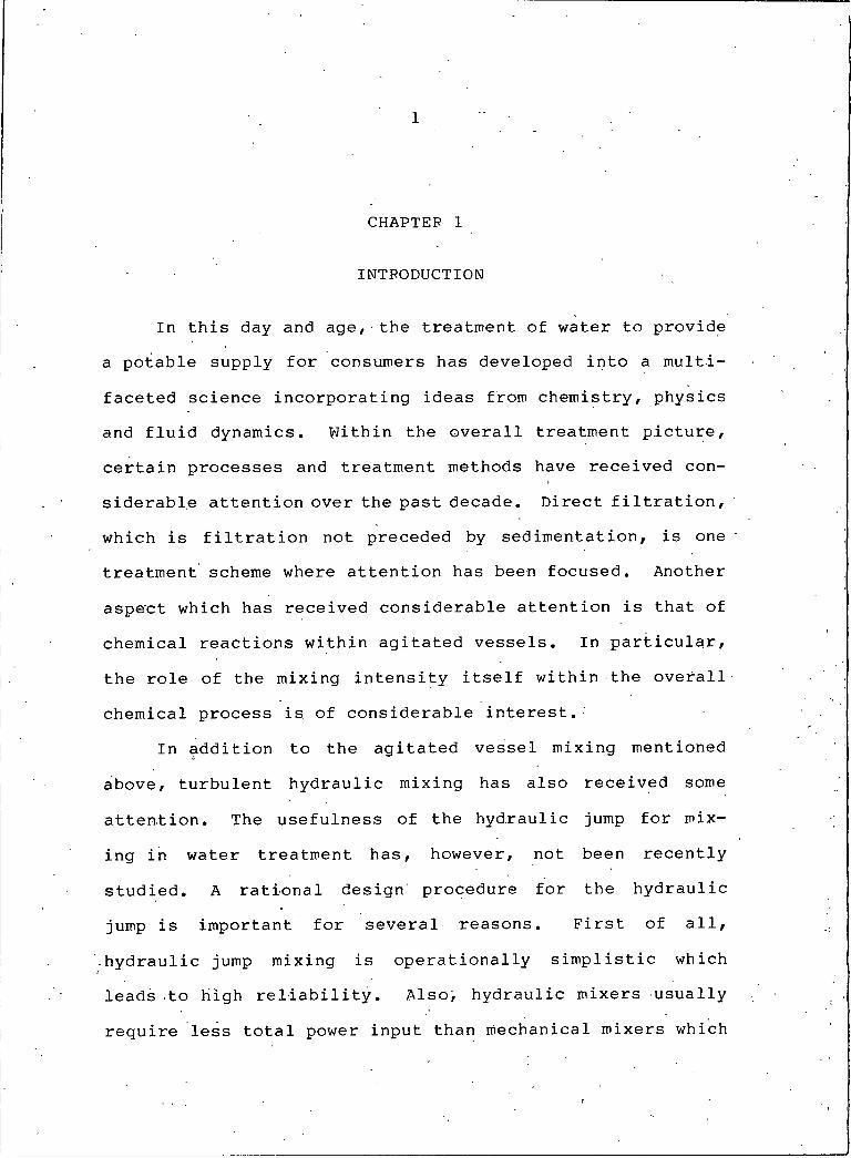
1. Power Dissipation Zones in a Stirred Tank(Cutter [5] ) ................ .. * ......... 7

2. Design and Operation Diagram for AlumT r e a t m e n t ....................................... 12

3. Idealized Colloid-Microscale InteractionVisualization ............... 17

4. Schematic Diagram-of Direct FiltrationPilot Plant ..................................... 23

5. Size Distributions for Turbidity Particles . . . 266. Details of Baffled Tank Reactor and Disc-

Turbine I m p e l l e r .............................. 287. Details of Hydraulic Jump F l u m e ......... .. . . 308. Details of Dual Media F i l t e r .................... 329. Residence Time Distributions for the

Baffled Tank R e a c t o r ......................... 4110. Residence Time Distributions for Two

Hydraulic J u m p s ................................ 4311. Typical Filter Data for Baffled Tank

Mixing with Alum Treatment ■ ’(n = 700 RPM) ................... . ............ .. 45

12. Typical Filter Data for Hydraulic JumpMixing with Ferric Chloride Treatment(Slope = 2.0 in/ft) ................ .. ... . . 46

13. Rate of Headless and Average EffluentTurbidity for Baffled Tank Mixingwith Alum Treatment .............. 48

14. Rate of Headloss and Effluent Turbidity.for Baffled Tank Mixing with FerricChloride Treatment ............ . . . . . . . 49

viiiLIST OF FIGURES— Continued

Page15. Rates of Headless and Average Effluent

Turbidity for Baffled Tank Mixingwith Ferric Chloride Treatment. .............. 51

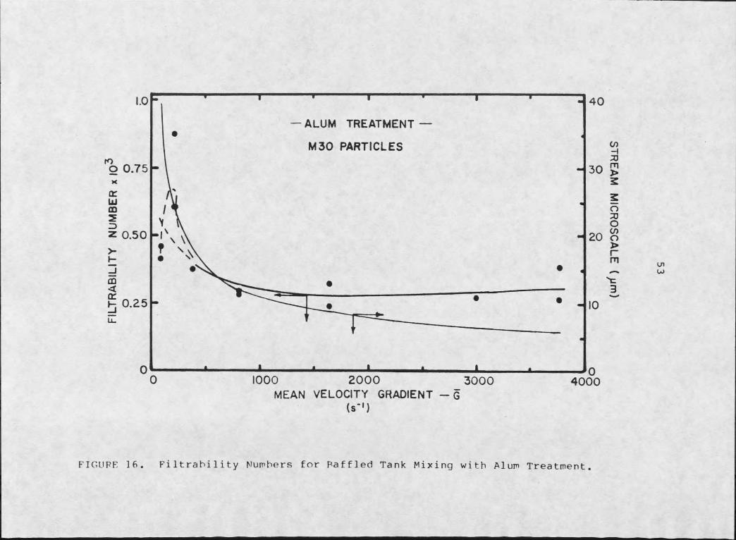
.16. Filtrability Numbers for Baffled TankMixing with Alum T r e a t m e n t .................. . 53

17. Filtrability Numbers for Baffled TankMixing with Ferric Chloride Treatment ;. . . . 54

18. Filtrability Numbers for Baffled TankMixing with Ferric Chloride Treatment . . . . 55

19. Rates of Headless for Hydraulic Jumpand Open Channel Mixing with FerricChloride Treatment ......................... * 59

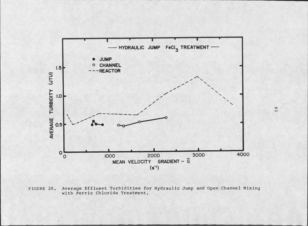
20. Average Effluent Turbidities for HydraulicJump and Open Channel Mixing withFerric Chloride Treatment .................... 61

21. Filtrabiiity Numbers for Hydraulic Jumjiand Open Channel Mixing with FerricChloride Treatment .............. ........... 62

22. Hydraulic Jump Length, L, for Jumps inSloping C h a n n e l s .............. .̂.............. 70

ix

LIST OF TABLES

< Page1. Water Analysis of Feed Water for Direct

Filtration Pilot Plant ....................... 242. Size Characteristics of Filter Media ........... 333. List of Pilot Plant Runs Including

Coagulant Dosages and pH Conditions ......... .364. Calculated Velocity Gradients for Baffled

Tank Mixer ................................ .. . 395. Calculated Velocity Gradients for Hydraulic

Mixers . * .................................... 406,. Mean Hydraulic Residence Times for Baffled

Tank Mixer ..................................... 427. Electrophoretic Mobility Data for Treatment

of M30 and SB325 Colloids . . . . . . . . 58

X

C

CoEijiF

FlGHip .

NoN

■ P

Po 0

ReTVV r

aId

gnnI , n2 ri r r2

NOMENCLATURE

Average effluent turbidity - TU Filter influent turbidity - TU Channel flow energy - ft Filtrability numberUpstream Froude number for hydraulic jumpAverage velocity gradient - s~lTotal filter headless at time T - inNumber; of particle collisionsNumber of colloid-microscale interactionsAverage power dissipated - ft*Ib/sPower numberFlow rate - cfsImpeller Reynolds numberFilter run length - hrPower dissipation volume - ft^Filtration rate - in/hr Colloid diameterImpeller diameter - ft; Water depth in flume-ft Acceleration of gravity - ft/s^Impeller speed - rev./s Colloid number counts Colloid radii -

xi

tu, v,X, y,Y2znE

Y yV

PB

NOMENCLATURE— Continued

Theoretical mixing time - V/0 - s w Respective velocity components z Respective coordinate directions

Water depth downstream of jump - ft Channel elevation - ft MicroscalePower dissipation per unit mass. - ft^/s^ Specific weight of water - Ib/ft^Fluid viscosity - lb•s/ft^Fluid kinematic viscosity - ft^/s Fluid density - slugs/ft3

SFlume slope angle

xi i

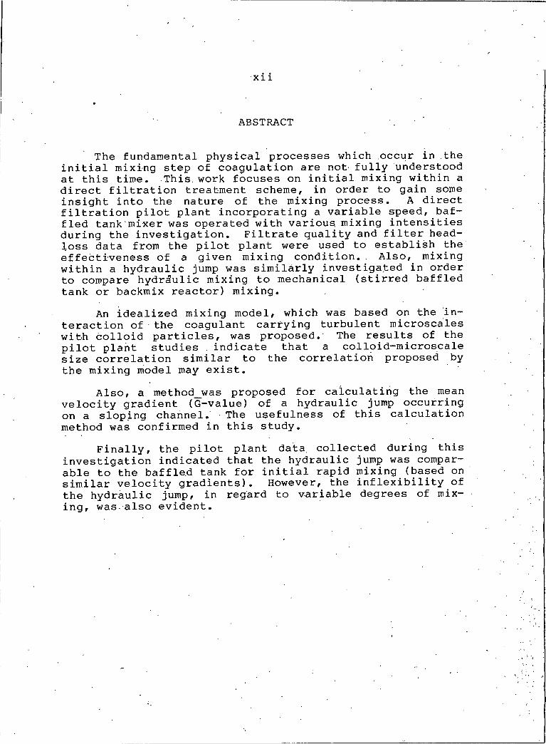
ABSTRACT

The fundamental physical processes which occur in the initial mixing step of coagulation are not fully understood at this time. This, work focuses on initial mixing within a direct filtration treatment scheme, in order to gain some insight into the nature of the mixing process. A direct filtration pilot plant incorporating a variable speed, baf­fled tank mixer was operated with various mixing intensities during the investigation. Filtrate quality and filter head- loss data from the pilot plant were used to establish the effectiveness of a given mixing condition. . Also, mixing within a hydraulic jump was similarly investigated in order to compare hydraulic mixing to mechanical (stirred baffled tank or backmix reactor) mixing.

An idealized mixing model, which was based on the in­teraction of the coagulant carrying turbulent microscales with colloid particles, was proposed. The results of the pilot plant studies . indicate that a colloid-microscale size correlation similar to the correlation proposed by the mixing model may exist.

Also, a method_was proposed for calculating the mean velocity gradient (G-value) of a hydraulic jump occurring on a sloping channel. The usefulness of this calculation method was confirmed in this study.

Finally, the pilot plant data, collected during this investigation indicated that the hydraulic jump was compar­able to the baffled tank for initial rapid mixing (based on similar velocity gradients). However, the inflexibility of the hydraulic jump, in regard to variable degrees of mix­ing, was also evident.

I

CHAPTER I

INTRODUCTION

In this day and age, the treatment of water to provide a potable supply for consumers has developed into a multi­faceted science incorporating ideas from chemistry, physics and fluid dynamics. Within the overall treatment picture, certain processes and treatment methods have received con­siderable attention over the past decade. Direct filtration, which is filtration not preceded by sedimentation, is one treatment scheme where attention has been focused. Another aspect which has received considerable attention is that of chemical reactions within agitated vessels. In particular, the role of the mixing intensity itself within the overall chemical process is of considerable interest.

In addition to the agitated vessel mixing mentioned above, turbulent hydraulic mixing has also received some attention. The usefulness of the hydraulic jump for mix­ing in water treatment has, however, not been recently studied. A rational design procedure for the hydraulic jump is important for several reasons. First of all, hydraulic jump mixing is operationally simplistic which leads to high reliability. Also, hydraulic mixers usually require less total power input than mechanical mixers which

2further enhance their operational attractiveness. The rea­son for the lower power requirements are two fold. First, the power dissipation volumes for hydraulic mixers are usu­ally much smaller than the volumes for mechanical mixers. Secondly, hydraulic mixers lack the frictional inefficien­cies common to motor driven mixers. There is no doubt that hydraulic mixing has its, share of drawbacks as well. The primary disadvantage with the hydraulic jump being the in­ability to change, the mixing intensity to accomodate varia­tions in the influent %ater quality.

The present study focused on initial mixing within a direct filtration treatment scheme. Both mechanical (stir­red baffled tank) and hydraulic (hydraulic jump) mixing were investigated. The importance of this study was based on the need for a better understanding of the initial mixing step of coagulation. This better understanding will, no doubt, lead to more efficient use of the employed in water treatment mixing operations.

energy

3

CHAPTER 2

OBJECTIVES

The overall objective of this study was to investigate the initial mixing step of coagulation and to gain some in­sight into the fundamental nature of the mixing process. The following were the specific objectives:

1. To study the initial mixing step of coagulation in a stirred baffled tank reactor in order to determine the role of mixing intensity in destabilization by charge neutralization using a direct filtration pilot plant.

2. To attempt to relate the results of the mixing study to the microscale of turbulence.

3. To propose a methodology for design of hydraulic jump mixers.

4. To compare hydraulic jump mixing with baffled tank (backmix) reactor mixing.

4

CHAPTER 3

PREVIOUS RELATED STUDIES

The theoretical studies which are related to this work can be divided into three categories. First ,, there is the material which deals with turbulence and mixing in general. Second, are the studies which have focused on mixing in the water treatment field. Both flocculation and initial mixing studies are of importance here. Finally, some aspects re­garding filtration analysis will be presented.

TURBULENT INITIAL MIXINGAs defined by Hinze [1] , turbulence is a flow condition

characterized by irregular motion in which various parameters vary in time and space. Hinze also points out that within the random variations, statistically distinct averages are obtainable. The concepts underlying turbulence, such as fluctuating velocities and turbulent intensities, are fully

z-' .developed in the literature [I, 2] and will not be discussed here. Of more concern to the present study, are the funda­mentals of energy dissipation, within a turbulent flow.

In any given turbulent flow it can be shown that regions of high velocity correlation exist. In a somewhat rough approximation, these regions where all the fluid exhibits

5

a similar velocity can he interpreted as eddies or vortices. Kolmogorof £ [3,4] was the first to rationalize turbulence from an eddy or length scale viewpoint by defining an in­tegral length scale and a microscale. The integral scale is related to large eddies which carry energy and the micro­scale is the eddy size at which energy dissipation by viscous friction begins. Kolmogoroff noted that these small eddies (microscale) would have to be in a state of equilibrium and their size would be a function of the energy input and the fluid viscosity. By dimensional analysis Kolmogoroff quantified the microscale as

n = (I)

where H is the microscale, V is the kinematic viscosity of the fluid and e is the power dissipated per unit mass.Since mixing is usually interpreted as being a function of power dissipation, it is the turbulent microscale which is of particular importance here.

Mixing in Baffled TanksSeveral ideas in regard to mixing in baffled tanks are

important to this investigation. First'there are the results of Cutter [5] which illustrate the nonuniformity of power dissipation within a baffled tank. Cutter found three distinct regions of power dissipation to exist within a

6baffled tank. He labeled the regions as the tip zone, the impeller stream zone and the bulk zone. Figure I illus­trates the three zones and the approximate power dissipa­tion within each zone, in relation to the mean dissipation. More recently, Okamoto, Nishikawa and Hashimoto [6] have con­firmed the existence of the impeller stream and bulk zones of a baffled tank as described by Cutter.

Long before Cutter's work. Camp and Stein [7] formulated the velocity gradient, or G—value, as a design parameter for determining the power requirements of a mixer. Camp and Stein utilized laminar fluid shear concepts to derive the

velocity gradient as

G = 0.5 (2 )

where G is the average velocity gradient, P is the power dis­sipated within volume V and U is the fluid viscosity. Camp and Stein also generalized the velocity gradient expression for turbulent flows by defining the root mean square (RMS) velocity gradient as

G 3v. 2 3x' + (3)

where u, v and w are the velocities in the x, y and z direc­tions respectively. Equation (2) thus represents an average value within a turbulent field.

ZONE OF MAXIMUM TURBULENCE

IMPELLER ZONE

TOTAL VOLUME = V= V, ♦ V3 Pm3 ^ ° - 25P

AVERAGE POWER DISSIPATION = P V3 ^ ° - 9V

FIGURE I. Power Dissipation Zones in a Stirred Tank (Cutter [5]).

8

Another parameter which is important in tank mixing is the dimensionless power number, P0 . Leentvaar and Ywema [8] explain the power number concept in detail and show the quantified expression as

where P is again the average power dissipated, p is the den­sity of the fluid, n is the impeller speed and d is the impeller diameter. For a given reactor^impeller configura­tion, the power number remains constant beyond a certain Reynolds number Re (̂ssIO4 for cylindrical baffled tanks) where

and all symbols are as previously defined. Thus, once the power number of a given reactor is known, power inputs and corresponding G-values can be computed for various impellers and rotation speeds.

Mixing in Hydraulic JumpsAt present, mixing in hydraulic jumps is somewhat less

well defined than mixing in baffled tanks. Chow [9] presents all the tools necessary to formulate a possible design ra­tionale. The hydraulic jump can be defined as the mechanism by which an open channel flow transforms from supercritical

— — I — 3 “5 P = Pp n d o (4)

Re- (5)

9

to subcritical flow.. Looking at the mixing capabilities of the jump from, a G-value standpoint, necessitates that the power dissipated within a specific volume be related to the jump characteristics.

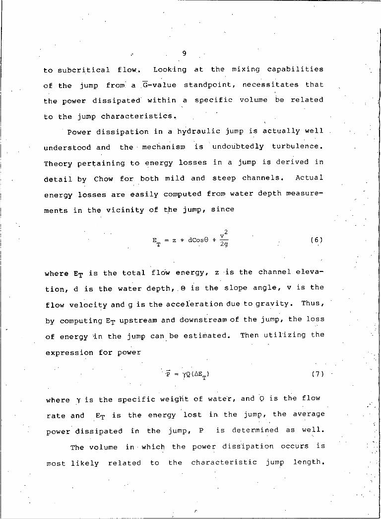
Power dissipation in a hydraulic jump is actually well understood and the mechanism is undoubtedly turbulence. Theory pertaining to energy losses in a jump is derived in detail by Chow for both mild and steep channels. Actual energy losses are easily computed from water depth measure­ments in the vicinity of the jump, since

2E = z + dCosG + — ( 6)T 2g

where E? is the total flow energy, z is the channel eleva­tion, d is the water depth,.6 is the slope angle, v is the flow velocity and g is the acceleration due to gravity. Thus, by computing Et upstream and downstream of the jump, the loss of energy in the jump can be estimated. Then utilizing the

expression for power

''-P = YQ(AEt) (7)

where y is the specific weight of water, and 0 is the flow rate and Et is the energy lost in. the jump, the average power dissipated in the jump, P is determined as well.

The volume in which the power dissipation occurs is most likely related to the characteristic jump length.

r

10

Chow illustrates that the jump ■ length L is a function'of the available flow energy (upstream Froude number and chan­nel slope) and presents empirical data which can be used to estimate the length of a jump which occurs in a sloping chan­nel. The actual power dissipation can then be assumed to occur in the fluid volume contained in the jump length L . Since the power and dissipation volume are known, a G-value for the jump can be computed.MIXING IN WATER TREATMENT

Mixing studies within the water treatment field are numerous, however, only a few studies are relevant here. These relevant investigations may be split into- those which have dealt with initial rapid mixing directly and those which have dealt with flocculation.

Initial Mixing StudiesWilson [10] attempted to define optimum rapid mixing by

studying the flocculation efficiencies resulting from two different mixing methods. The actual optimization was based on a floe strength model where optimum mixing was de­fined as the condition which produced the strongest floes within the flocculator. Wilson employed a baffled tank reactor and.a tubular reactor in his studies and concluded that uniform, instantaneous, plug-flow mixing was the opti­mum condition based on floe strength.

J

11

Sometime later, Stenquist and Kaufman [11] completed a series of continuous flow experiments in which they com­pared a flash mixer (backmix) to a. multiple orifice grid mixer (pipe flow). Their results produced no conclusive evidence that backmixing was inherently inferior to plug- flow mixing for alum treatment-, when flocculation effic­iency was used as the gauge. ■ Even though Stenquist and Kaufman's conclusions seem to contradict those• of Wilson, the results of both studies may have been more a function of alum coagulation chemistry than of mixing itself. The actual effects of alum dosage in relation to mixing are dis­cussed below.

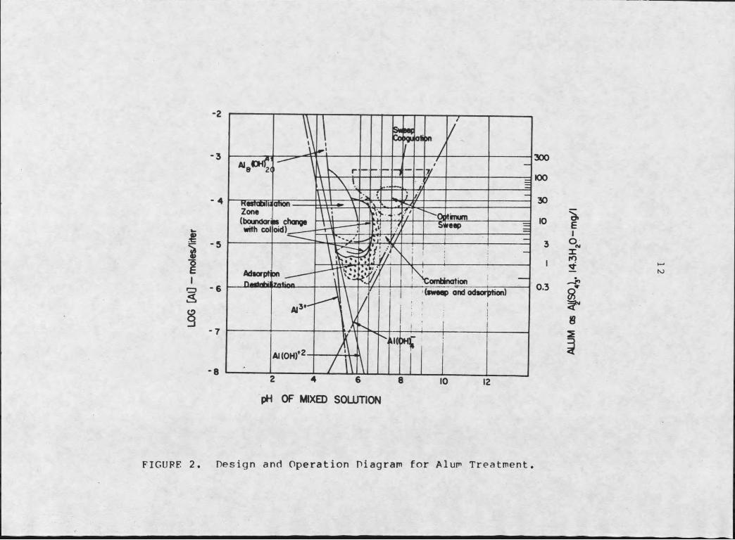
Amirtharajah and Mills [12] developed the design diagram for alum treatment as shown in Figure 2. The diagram is based on thermodynamic principles and delineates the region of solid phase aluminum hydroxide as a function of pH. Also shown on the diagram are regions where specific coagulation mechanisms predominate. Amirtharajah and Mills then applied the diagram to rapid mixing by performing jar tests with various degrees (G-values) of rapid mixing. They concluded that intense, short duration mixing was. essential if adsorp­tion-destabilization was the primary mechanism of coagul­ation. They also found that when sweep coagulation was the predominant mechanism, mixing effects were minimal. It is important to note, that Wilson and Stenquist both operated

Co Kju afi>n

Zone (boundori with col

Adsorption

pH OF MIXED SOLUTION

IOO30IO3I

0.3

300

FIGURE 2 Design and Operation Diagram for Alum Treatment

ALJUM

os Aj(SO4)s. l4.3H20-mg/l

13

their mixers in the sweep zone during their investigations. Amirtharajah [13] also suggested that a fundamental size relationship between the turbulent microscale and the par­ticles which were to be destablized may exist.

Only one investigation of the hydraulic jump's effec­tiveness as an initial mixer has been reported. . Levy and Ellms [14] conducted full scale alum treatment studies utilizing a hydraulic jump for rapid mixing. They concluded that the hydraulic jump was a very effective means for mixing coagulants. For the energy expended. Levy and Ellms concluded that the jump produced mixing of great rapid­ity and thoroughness.

Turbulent FlocculationOf primary importance to this investigation are particle

collision theories which were first, introduced by von Smolu- chowski [15] . He derived the collision theories for laminar shear but the original formulations have now been generalized for turbulent flow conditions. Saffman and Turner [16] uti­lized Smoluchowski's ideas to predict.the collision of fain droplets in a turbulent cloud. They quantified the number of collisions, N0 , as

' .3 Sire 0.5 .Np = nln2(rl + r 2 (l5^'

(8)

14where and ng are respective drop number counts, rj and r2 are respective drop radii, and all other symbols are as pre­viously defined. Spielman [17] has also pointed out that Saffman and Turner's Equation (8) is applicable to turbulent flocculation. Most recently, Adler [18] has incorporated Smoluchowski's ideas into, a general particle collision theory which incorporates hydrodynamic effects as well as electric field, double layer and Van der Waals' forces. He subdivides coagulation into homocoagulation and heterocoagu­lation, where homo^ refers to coagulation of equal-sized particles and hetero- refers to coagulation of unequal­sized particles. Adler concluded that homocoagulation is almost always better, at least within the chemical and physical constraints of his develdment. Considering, all the above studies, von Smoluchowski's ideas, and their extension to turbulent flow, seem to be far reaching and may thus be applicable to the rapid mixing process.

FILTRATION ANALYSISSince this study is not an investigation of filtration

fundamentals per se, the only literature of interest is that which deals with analysis of filtration data. The overall response of a filter to the depostion of mass within the media is a function of both headless and effluent quality. Several researchers have attempted to define the response of a filter to mass loading by combining headless and efflu­

15

ent quality data into a single filtrability index [19, 20, 21, 22, 23]. Recently, Janssens, Adam and Buekens [24] did a statistical analysis on various filtrability indexes uti­lizing direct filtration pilot plant data as a base. They were interested in determining which index would be the best tool for filter response analysis. They concluded that the Filtrability Number, proposed by Iyes [21] , was the most useful. The expression for the Filtrability Number F , is given by

F VV r

(9)

where T is the filter run length defined by effluent quality degradation, Ht is the total headloss at time T , C is the average filter effluent turbidity through time T , C0 is the filter influent turbidity and V is the filtration rate. Consistent units make F a dimensionless parameter. Close inspection of the arrangement of the individual parameters in the' expression for F , leads to the. conclusion that when F is minimized, an optimum filtration condition exists.

16

CHAPTER 4

IDEALIZED MIXING MODEL

The first step in developing an idealized mixing model involved a visualizatiori process whereby the micro­scopic aspects underlying mixing could be postulated., Since mixing is most often associated with power dissipation, in­teractions between colloid particles in suspension and the turbulent microscale can be rationalized as being of primary importance. . The visualization was confined to a homogeneous turbulent field consisting of eddies whose size could. be represented by the microscale formulation (I). Also, the development was restricted to the adsorption-destabilization process where a uniform particle suspension was to be treated with a,chemical coagulant. Furthermore, the micro­scale eddies in the field were assumed to be responsible for the transport of the coagulant hydrolysis species, which are most likely in incipient form.

Turning to the visualization. Figure 3 illustrates two simplistic particle-microscale interaction possibilities. Case I represents a condition where the microscale is much larger than the colloids and thus, the particles are imbed­ded within the eddy. Particles in the eddy will experience a laminar like shear field and are also exposed to the coagu-

MIC

RO

SC

ALE

\

CO

LLO

ID D

IA.

a

IDEALIZEDMICROSCALE-COLLOID

INTERACTION

© COLLOID

COAGULANT

CASE 2

t) I r 2I - ^

O

POWER DISSIPATION

FIGURE 3. Idealized Colloid-Microscale Interaction Visualization

18

Iant. Under the conditions of Case I, the efficiency of the rapid mix (based on destabilization) would seem to be con­trolled by the coating, mechanisms which cause the coagulant to be adsorbed onto the colloid. The exact nature of the coating mechanisms is presently not fully understood.

As more power is made available to the system, a tran­sition is made to smaller and smaller eddies. Finally, the condition exists where the microscale and colloids are equal in size and this condition is shown as Case 2 in Figure 3. The Case 2 condition is such that the particles and eddies can be considered as separate entities and in order for the colloids to be exposed to the coagulant, a collision of sorts must occur. Thus, the efficiency of mixing in the Case 2 situation may be controlled by a collision or inter­action phenomenon.

In looking more closely at the transition zone between Case I and Case 2, Amirtharajah [25] has proposed the fol­lowing colloid-microscale interaction theory. The basis of the idea was that for colloid destabilization to occur, the colloid particles must be coated with the positively charged aluminum hydroxide solid phase species which are in- cipiently formed in the fluid. These species have to be transported by the fluid eddies so that they will interact with the colloid particles.

19Starting with Saffman and Turner's Equation (8), which

is applicable for the condition where the turbulent micro­scale is larger than the particles and with some minor re­arrangement.

N = Icn1Ii2 Ca1 + n)3 (̂ ) (10)

I

where N is the number of colloid-microscale interactions, k is a constant, ai is the colloid diameter, n is the micro­scale, v is the fluid kinematic viscosity, e is the power dissipation per unit mass and ni and t\2 are the colloid and microscale number counts respectively. Within a given mixer, the number count of colloids can be considered con­stant. Furthermore, in this first approximation model, the number count of microscale eddies is assumed constant, even though there is little doubt that as the size of the microscale is reduced, the number count of eddies will in­crease within the mixing ' volume. With the above assump­tions, Equation (10) is reduced to the form

N = k1 (a1 + n)3(^)°*5 (ID

20

Rearranging the microscale expression, Equation (I), in the form

e =

and substituting into Equation (11) yields

(12)

N = R1Vta1 n)3'(i)2 (13)

The fluid viscosity is assumed to be independent of q and is, therefore, incorporated into the constant yielding

3,1.2N = R2 (a1 + n) (̂ ) (14)

as the proposed mixing theory expression.In order to identify the extreme points of the mixing

theory, Equation (14) was expanded and differentiated with respect to n giving

dNdn 4 - > 2 (15)

21

Setting Equation (15) equal to zero leads to

ai T aI 22 (-^) 3 + 3 " I = 0 (16)

and a real root of (a]/n) = 0.5. Taking the second deriva­tive of Equation 14,

and substituting = 0 . 5 n gives a positive value forEquation (17) for all n indicating a minimum for Equation 14. Thus, when the microscale is twice the colloid size a minimum number of colloid—microscale interactions should

occur.Although the above derivation is not complete or rig­

orous, as a first approximation, it provides some interest­ing insights into the initial mixing process.

3 - 4 2 - 36k2 (ajn + a^n ) (17)

22

CHAPTER 5

EXPERIMENTAL WORK

PLANThe experimental portion of this study consisted pri­

marily of measuring the response of a dual media filter to various methods of rapid mixing the coagulant. Both mechan­ical and hydraulic mixing were utilized during the investi­gation. A baffled tank reactor served as the mechanical mixer and hydraulic mixing was provided by a flume apparatus. Mixing within the flume was produced by either turbulent open-channel flow or a hydraulic jump.

The sensitivity of a dual media filter to small changes in the characteristics of its influent suspension is well known [26] . Thus, the filter makes an ideal gauge for measur­ing the effectiveness of the rapid mix.

DIRECT FILTRATION PILOT PLANTA direct filtration pilot plant was constructed in order

to study the initial mixing step of coagulation. Figure 4 illustrates the pilot plant flow scheme. A constant flow of 2.0 gpm (8 gpm/ft2 filtration rate) was maintained through all pilot plant runs. Both hot and cold, tap water were used to insure constant temperature conditions. A Powers Foto-

A. THERMAL BLENDING VALVEB. 20 MICRON FILTERC. RAW WATER PREPARATIOND. BUFFER FEEDE. TURBIDITY FEEDF. COAGULANT FEEDG. RAPID MIXERH. DUAL MEDIA FILTER

0 - PUMP 0 FLOW METER

h c

BACKWASH

WASTE

FIGURE 4 Schematic Diagram of Direct Filtration Pilot Plant

24guard Model 440-1500 thermostatic blending valve mixed the hot and cold streams to provide the constant temperature feed water. The temperature of the feed water was 80°F for all plant runs. A chemical analysis of the feed water was performed during the investigation and the results are listed in Table I.Table I. Water Analysis of Feed Water for Direct Filtration

Pilot Plant.

PARAMETER QUANTITY

Total Hardness 105 mg/1 as CaCOgTotal Alkalinity 80 mg/1 as CaCOgTotal Dissolved Solids 150 mg/1Turbidity 0j5 to 1.0 TUPH 7,4 - 7.7

-2SO4 8.0 mg/1— 3PO4 <0.2 mg/1

None of the analysis results are particularly significant except for the sulfate concentration of 8.0 mg/1. Sulfate concentrations of 8.0 mg/1 and up have been shown to have a considerable impact on the effectiveness of alum when it is , used as a coagulant. It is believed that the sulfate anion neutralizes the charge on the aluminum hydroxide solid phase . which greatly reduces its destabilization potential [27] .

The remainder of the raw water preparation was carried out in a 20 gallon continuously stirred tank. The raw.water tank was fed continuously with the constant temperature.feed water as well as a turbidity slurry and pH buffer solution.

25

Hydrochloric acid (Baker Reagent, 37% HCl), at a concentra­tion of 30 milliliters acid per liter of water, was used for the buffer solution. Feeding the buffer into the raw water tank provided a near constant raw water pH through all plant runs.

A suspension of Min-U-Sil (Si0 2 ) was used for the tur­bidity slurry. Two different particle size distributions were used in the experimental work and Figure 5 illustrates the distributions. . It is important to note that distribu­tions by weight as well as distributions by particle num­bers are shown in Figure, 5. The weight distributions were obtained by standard hydrometer tests. (ASTM D422) . An Omnimet Image Analyzer (IA) by Buehler (Bausch & Lomb) was employed to provide the number count distributions. The IA consists of a microscope which is coupled to a visual monitor. The lA's electronics scan for shading differentiation (par­ticles against background) and then count the particles which are greater than a specified size.

Samples for"the IA were diluted samples of the turbidity slurry. The IA samples were analyzed in suspension form be^ cause drying the samples caused particles to agglomerate which led to erroneous results.

The Min-U-Sil material itself is a product of the Pen­nsylvania Glass Sand Corporation (PGS). Min-U-Sil 30 (M30), the coarsest grind manufactured by PGS, served as one of

PER

CEN

TAG

E FI

NER

26

A SB325 A• M 30 o

A o % BY WEIGHT Ae % BY NUMBER

PARTICLE SIZE (;jm )

FICUPE 5. Size Distributions for Turbidity Particles.

27the particle distributions. The other distribution, SB325, was obtained from Berkeley 325 which is the, feed stock for the M30 grinding mills.. A sedimentation process, outlined below, was employed to produce the SB325 from the Berkeley 325 material.

Suspensions of 50 grams per liter of Berkeley 325 were prepared in 5 gallon buckets and allowed to sit for one hour. The particles which settled in this time period were col­lected and dried resulting in the SB325 distribution. This sedimentation process was developed based on the ASTM D422 hydrometer test and was designed to remove a major fraction of the particles smaller than 5 micrometers.

From.the raw water tank, the water proceeded to the rapid mix unit where either alum (AlgfSO^j^'lGHgO) or ferric chloride (FeCl3 was introduced to destabilize the sus­pension, by charge neutralization. After rapid mixing, the destabilized suspension passed directly into the dual media filter. The details of each of the- rapid mix units, as well as the details of the filter, are described below.

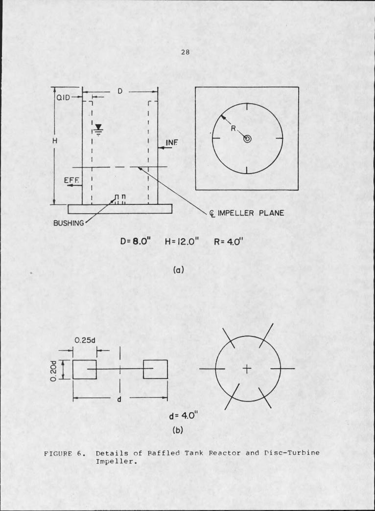
Baffled Tank ReactorBased on the designs of other research [5, 6 , 8 ] and

scale up considerations, the baffled tank reactor was con­structed as shown in Figure 6.. Also shown in Figure 6 are the details of the discturbine impeller which was used for mixing in the baffled tank. Both the tank and the

POZ O

28

IMPELLER PLANEBUSHING

D= 8 .0 H= 12.0 R= 4.0

(a)

FIGURE 6 . Details of Baffled Tank Reactor and Disc-Turbine Impeller.

/

29impeller were constructed of plexiglas.

A constant water depth of 8.0 inches was maintained in the reactor during all pilot plant runs. The influent to the reactor was fed 6.0 inches above the reactor bottom and the effluent was drawn off 2.0 inches above the bottom. This reactor configuration forces all the flow to pass through the impeller plane center line which was 4.0 inches above the bottom. The coagulant was fed into the reactor system on the impeller plane center line at a point 0.25 inches from the blade tips. A Bodine NHS-54 variable speed motor was used to drive the impeller.

Details of FlumeAs a comparison for the baffled tank, a hydraulic mix­

ing device which incorporated a narrow flume and a hydraulic jump was constructed. Figure 7 illustrates the flume con­figuration and all important dimensions. Various channel slopes could be attained by adjusting the position of a sliding block on the aluminum base. Slopes of 1.5, 2.0,2.5 and 3.5 inches per foot were utilized in the experiments. These slopes produced highly turbulent, supercritical flow conditions within the channel. By inserting a barrier in the channel, which essentially acted as a sluice gate, a hydraulic jump could be produced.

FIGUPF 7. Details of Hydraulic Jump Flume.

31The flume-jump apparatus was placed in exactly the same

location as the.baffled tank within the overall plant scheme.. Raw water entered the channel via a stilling basin filled with stones to disperse the flow. Once the water passed in-

v *to the channel section it was destabilized by the addition of the coagulant. When a hydraulic jump was being used, the coagulant feed point was approximately 1.5 inches upstream of the jump toe. During plant runs where the channel flow alone provided the mixing, the coagulant feed point was mid­way along the channel length. It should be noted, that the flume was used to treat the M30 suspension only. Finally, the destabilized suspension passed directly into the filter rise tube as shown in Figure 7. - . .

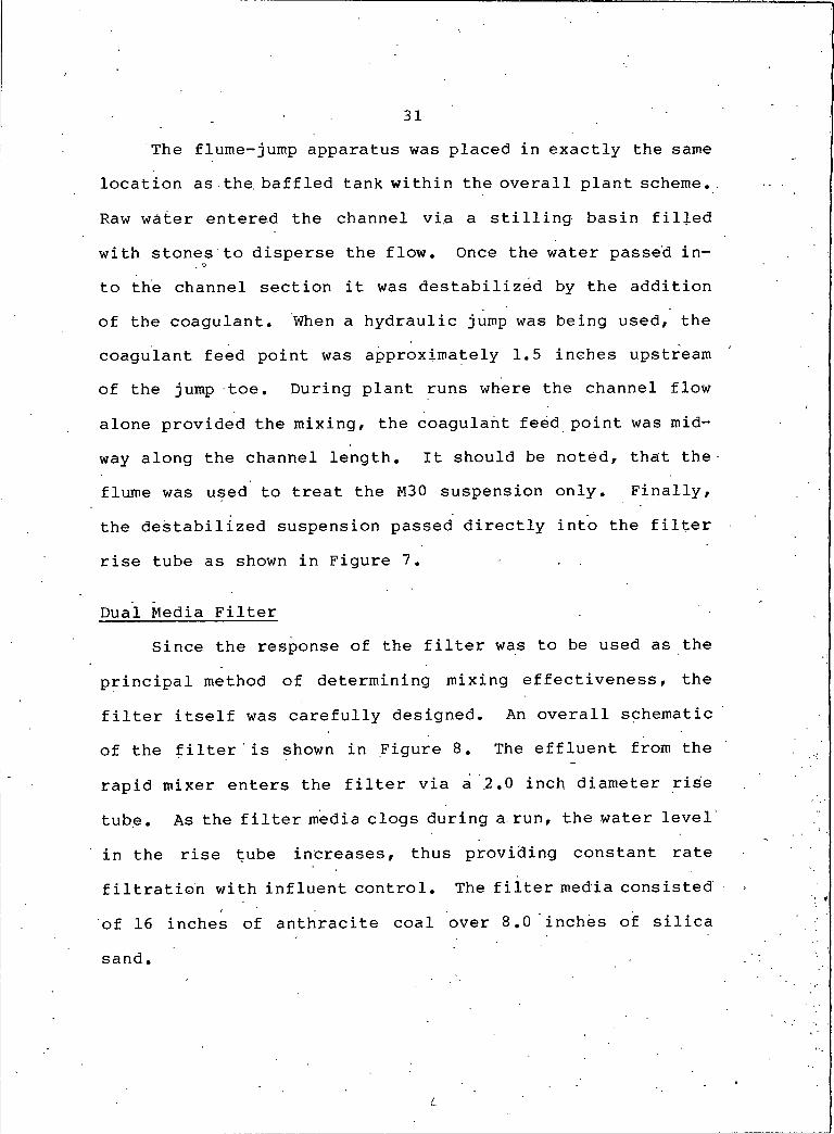
Dual Media FilterSince the response of the filter was to be used as the

principal method of determining mixing effectiveness, the filter itself was carefully designed. An overall schematic of the filter is shown in Figure 8 . The effluent from the rapid mixer enters the filter via a 2.0 inch diameter rise tube. As the filter media clogs during a. run, the water level in the rise tube increases, thus providing constant rate filtration with influent control. The filter media consisted of 16 inches of anthracite coal over 8.0 inches of silica sand.

L

32

INFLUENT

RISE TUBE

BACKWASH

FILTER BOX

LEVELS

COAL -

• SAND

I I I I IMANOMETER

BOARDDRIP SAMPLES

ORIFICE PLATE - BACKWASH EFFLUENTUNDERDRAIN

FIGURE 8 Details of Dual Media Filter

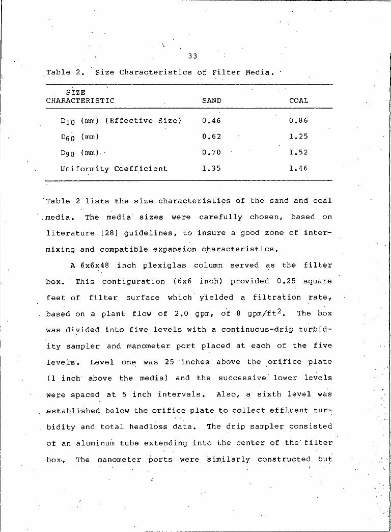
33Table 2 . Size Characteristics of Filter Media.

SIZECHARACTERISTIC SAND COAL

D 10 (mm) (Effective Size) 0.46 0.8 6

d6 0 (mm) 0.62 1.25

d90 (mm) ■ 0.70 1.52Uniformity Coefficient 1.35 1.46

Table 2 lists the size characteristics of the sand and coal media. The media sizes were carefully chosen, based on literature [28] guidelines, to insure a good zone of inter­mixing and compatible expansion characteristics.

A 6x6x48 inch plexiglas column served as the filter box. This configuration (6x6 inch) provided 0.25 square feet of filter surface which yielded a filtration rate, based on a plant flow of 2.0 gpm, of 8 gpm/ft^. The box was divided into five levels with a continuous-drip turbid­ity sampler and manometer port placed at each of the five levels. Level one was 25 inches above the orifice plate (I inch above the media) and the successive lower levels were spaced at 5 inch intervals. Also, a sixth level was established below the orifice plate to collect effluent tur­bidity and total headless data. The drip sampler consisted of an aluminum tube extending into the center of the filter box. The manometer ports were, similarly constructed but

.

34only projected 0.5 inches into the media. A plexiglas plate with twenty five 0.25 inch diameter holes was used for the orifice plate. The function of the orifice plate was to sup-

VIport the media (in addition to a nylon mesh) and to provide

even filtration. Also, the orifice plate provided even dis­persion of the backwash water during cleaning.

Cleaning of the filter was systematically performed by using both air scour and water backwash. Air was blown intp the submerged filter media through each of the drip samplers. The necessity for air scour was established after water wash­ing alone proved to be ineffective in breaking up the chunks of material which were sheared off the media.x After the air flow was stopped, the filter was washed with water for an ex­tended period of time.. The washing flow rate employed was sufficient to provide a fifty percent expansion of the bed.

FILTER PERFORMANCE DATATo insure the stability of the pilot plant and to

determine the filter response, various physical and chemical parameters were recorded at half hour intervals throughout each run. Measurements of pH were made on the raw water and filter effluent (level 6 ) in order to maintain constant chemistry within the flow system. An Altex digital pH meter from Beckman Instruments was used for all the pH measure­ments. Also, the raw water turbidity was monitored to insure constant mass loading of the rapid mixer and filter.

35Filter response to the various rapid mix conditions was

established by recording the turbidity of the water from each of the drip samplers. In addition to the turbidity data, headless data was obtained by monitoring the total available head at each level in the filter.

The electrophoretic mobility of the particles after de- stabilization (level I) was also monitored as a secondary parameter. A G.K. Turner Zeta Meter was employed to measure the mobility of the particles. The mobility measurement pro­cedure consisted of recording the. average mobility of ten particles found in each of the samples collected at half hour intervals. The ten particles were randomly selected to reflect the range of mobilities and particle sizes that were seen in the sample.

A list of all the pilot plant runs, including coagulant dosages and pH conditions can be found in Table 3. The total number ■ of plant runs where . coagulant was used was thirty-eight. An additional run without coagulant was also made in order to establish the filter's baseline removal efficiency. All the pilot plant runs were between three and five hours in length.

36Table 3. List of Pilot Plant Runs Including Coagulant

Dosages and pH Conditions.

COAGULANT - VELOCITY NUMBERDOSAGE/ MIXER GRADIENT-G OFCOLLOID (s-1 ) RUNS

75 2Alum- Baffled 210 2

8 mg/1 @ pH 6.9 38 5 ITank 810 2

M30 1640 23000 I3800 2

75 2Ferric Chloride Baffled ' 210 I8 mg/1 @ pH 6.2 810 I

Tank 1640 IM30 2290 2

3000 I ,3800 , 2

Ferric Chloride Baffled 210 28 mg/1 @ pH 6.3 810 2

Tank 1640 2SB325 3000 I

3800 I

Ferric Chloride Hydraulic 705 I8 mg/1 @ pH 6.2 690 I

Jump 680 IM30 870 I

Ferric Chloride Open 1080 I8 mg/1 @.pH 6.2 1360 I

Channel 1700 IM30 2300 I

Alum Dosage = 8 mg/1 as Al2 (SO4)3-14.3H20Ferric Chloride Dosage = 8 mg/1 as FeCl3 *6H20

37DYE TRACE STUDIES

In order to determine the macroscopic mixing character­istic of both the baffled tank and the hydraulic jump, stan­dard dye trace studies were performed. By utilizing fIuor- ometric techniques and common analysis procedures explained by Weber [29], a fairly good representation of the residence time distribution (RTD) for the given mixer was obtained. Weber also explains a numerical integration procedure which yields the centroid of the RTD. By definition, the centroid of the rector RTD is the mean hydraulic residence time (MHRT) for the reactor. Furthermore, Weber illustrates a theoret­ical RTD calculation for a complete mix reactor.

Rhodamine WT , a nonreactive fluorescent dye, was used in the tracer studies. During the tracer studies, the dye was introduced into the mixers as a pulse, via the coagu­lant feed conduits. Samples were collected from the mixer effluent after the dye was injected and analyzed on a G.K. Turner Fluorometer. The fluorometer detected Rhodamine' WT at concentrations as low as 0.0001 mg/1. The data from the fluorometer was later plotted and statistically analyzed as a described by Weber [29], to establish the mean hydraulic residence time for the given mixer.

38

CHAPTER 6

RESULTS AND DISCUSSION

The results of this investigation fall into three major categories. First> there is the calculated mixing parameters for the various mixers. Secondly, the pilot plant data and filtration results are considered. Finally, the hydraulic and mechanical mixer comparisons are made.

CALCULATED MIXING PARAMETERSThe parameters which were chosen to describe the mixing

in the baffled tank and hydraulic jump were mean hydraulic residence time (MHRT) and the average mixer, velocity gradient (G) . For comparison purposes, Gt values have also been cal­culated. the value of t used was V/Q for the reactor. In regard to the hydraulic jump, t was assumed equal to the MHRT for the given jump. The methods for calculating the MHRTs and G-values were outlined in the. Previous Related Studies section and the following paragraphs focus on the results of the above mentioned calculations.

Velocity GradientsPower dissipation within the baffled tank can be calcu­

lated by using the power number Equation (4) once the reac­tor power number is known. Leentvaar [8 ] reported that the

I

power number for a cylindrical baffled tank, with a disc impeller, was 5.0. It is important to note that power losses computed using the power number expression represent average losses within the entire tank volume. Thus, by using the power number losses in the expression for G, Equation (2) , an average velocity gradient for the baffled tank can be found. Table 4 lists the results of the power loss, G-value and Gt-value calculations for the baffled tank.

39

Table 4. Calculated Velocity Gradients for Baffled Tank.

IMPELLERRPM

POWERDISSIPATION (ft'lbs/s)

VELOCITY GRADIENT-G

(s-1 ) 'Gt

50 0 .0.2 , 75 3,900100 0.18 210 10,900150 0.62 385 20,000250 2.74 810 42,100400 11.21 1640 85,300500 21.90 • 2290 119,100600 37.84 3000 156,000700 60.09 3800 197,600

G-values and Gt values for the hydraulic jump and openchannel, for various channel slopes , are shown in Table 5.A sample calculation of the power loss and the G-valuefor the jump can be found in the Appendix. It should be noted here that the open channel G-value for the 3.5 inches per foot slope, may be in error. The reason for the error is related to the extreme curvature of the water surface in the flume at this large slope. Since the flume was only

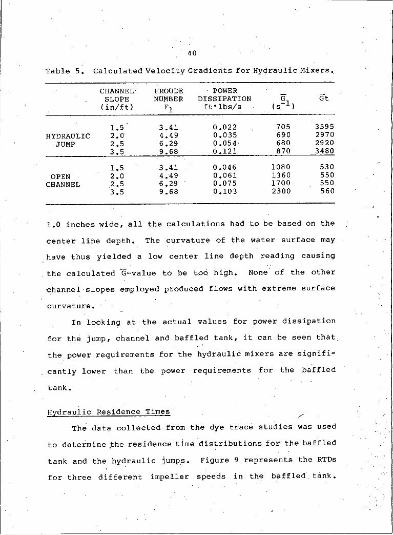
40Table 5. Calculated Velocity Gradients for Hydraulic Mixers.

CHANNEL FROUDE POWER -SLOPE NUMBER DISSIPATION G, Gt(in/ft) F1 ft•Ibs/s (s-1 )

■ 1.5 3.41 0.022 705 3595HYDRAULIC 2.0 4.49 0.035 690 2970

JUMP 2.5 6 .29 0.054 680 29203.5 9.68 0.121 870 34801.5 3.41 . 0.046 1080 530

OPEN 2.0 4.‘4 9 0.061 1360 550CHANNEL .2.5 6.29 0.075 1700 550

3.5 9.68 0.103 2300 560

1.0 inches wide, all the calculations had to be based on the center line depth. The curvature of the water surface may have thus yielded a low center line depth reading causing the calculated *G-value to be too high. None of the other channel slopes employed produced flows with extreme surface curvature. '

In looking at the actual values for power dissipation for the jump, channel and baffled tank, it can be seen that the power requirements for the hydraulic mixers are signifi­cantly lower than the power requirements for the baffled tank.

Hydraulic Residence Times . .The data collected from the dye trace studies was used

to determine the residence time distributions for the baffled tank and the hydraulic jumps. Figure 9 represents the RTDs for three different impeller speeds in the baffled, tank.

O &

4

AA N= 50 RPM

\ A O N = 100 RPM\

X/ >

O N = 700 RPM— — — THEORETICAL

B x

O 50 ' 100 150TIME (SEC)

FIGURE 9. Residence Time Distributions for the Baffled Tank ReactorD P

O

42

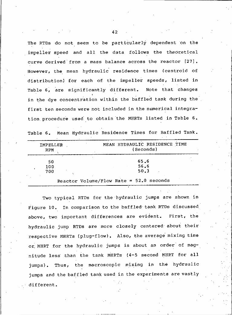
The RTDs do not seem to be particularly dependent on the impeller speed and all the data follows the theoretical curve derived from a mass balance across the reactor [27] . However, the mean hydraulic residence times (centroid of distribution) for each of the impeller speeds, listed in Table 6 , are significantly different. Note that changes

Iin the dye concentration within the baffled tank during the first ten seconds were not included in the numerical integra­tion. procedure used to obtain the MHRTs listed in Table 6 .

Table 6 . Mean Hydraulic Residence Times for Baffled Tank.

IMPELLER . RPM \

MEAN HYDRAULIC RESIDENCE TIME (Seconds)

50 65.6100 56.6700 \ 50.3

Reactor Volume/Flow Rate = 52.0 seconds

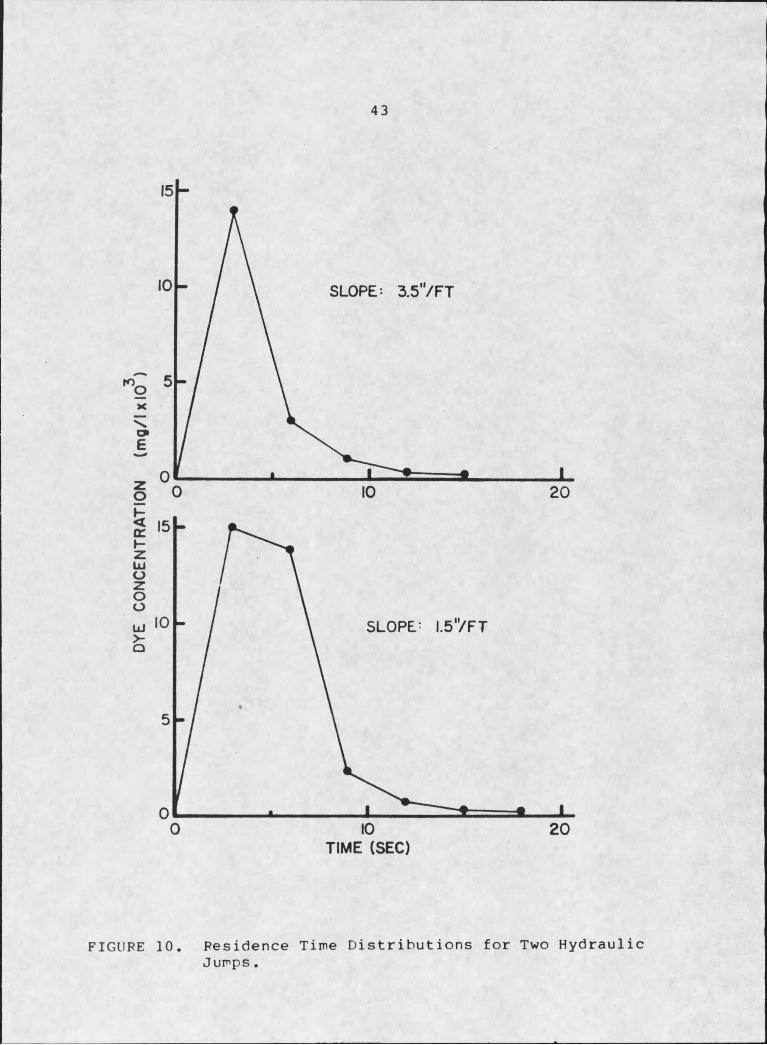
Two typical RTDs for the hydraulic jumps are shown in Figure 10. In comparison to the baffled tank RTDs discussed above, two important differences are evident. First, the hydraulic jump RTDs are more closely centered about their respective MHRTs (plug-flow). Also, the average mixing time or, MHRT for the hydraulic jumps is about an order of mag­nitude less than the tank MHRTs (4-5 second MHRT for all jumps). Thus, the macroscopic mixing in the hydraulic jumps and the baffled tank used in the experiments are vastly

different.

DYE

CO

NC

ENTR

ATI

ON

(m

g/l

xIO

)

43

SLOPE- I.57FT

O IO 20TIME (SEC)

FIGURE 10. Residence Time Distributions for Two Hydraulic Jumps.

44FILTRATION RESULTS

As outlined in the Experimental Work section, the raw filter data consisted of various turbidity and headless readings. The turbidity data will be referenced directly by v the level (1-6) from which the sample was taken. Head-. loss data on the other hand, is coded by referring to the levels through which the loss occurred. For example, the headless in the uppermost layer of coal would be Hl-2 and the total headless would be Hl-6 (see Figure 8 ).

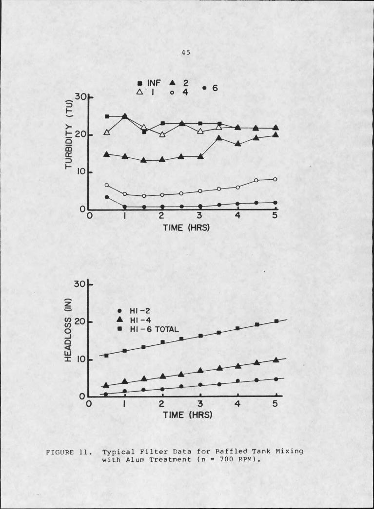
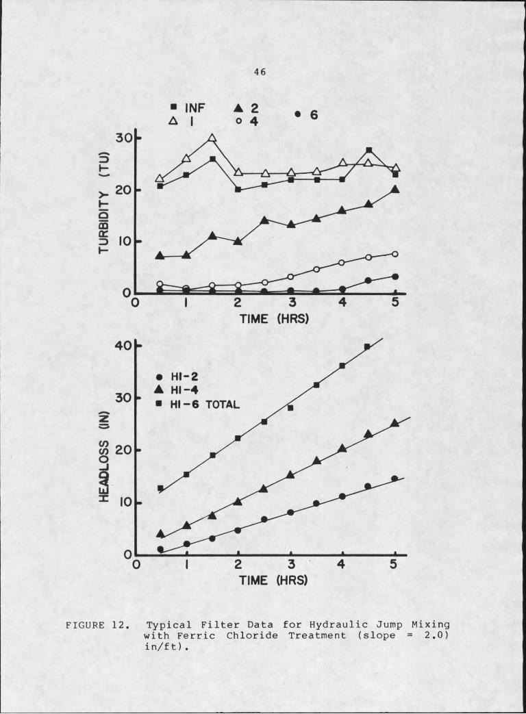
Two typical examples of raw filter data are shown in Figures 11 and 12. The top graph in each figure, shows the turbidity removal as a function of time and the lower graph illustrates the corresponding headlosses. Note that the headless lines are very linear, which is characteristic of a stable well designed filter system with good depth removal. A single plant run was also made in which no coagulant was added. This no treatment run was performed in order to establish a base for the other plant runs. The results of the no coagulant run showed that the filter would not re­move any of the nondestabilized material. This also led to a zero headless buildup.

Filter Response to Baffled Tank MixingAs a first attempt to define the effectiveness of vari­

ous mixing conditions for. the baffled tank, the rate of head- loss buildup and average effluent turbidity for each run was

HEA

DLO

SS

(IN)

TUR

BID

ITY

(T

U)

45

■ INF ▲ 2

TIME (HRS)

• HI - 2 A HI - 4 ■ HI - 6 TOTAL

TIME (HRS)

FIGURE 11. Typical Filter Data for Baffled Tank Mixing with Alum Treatment (n = 700 PPM).

HEA

DLO

SS

(IN)

TUR

BID

ITY

(T

U)

46

■ INF A 2A l o 4 • 6

TIME (HRS)

• H I-2 A H I-4 ■ H I- 6 TOTAL

TIME (HRS)

FIGURE 12. Typical Filter Data for Hydraulic Jump Mixing with Ferric Chloride Treatment (slope = 2.0)in/ft) .

47 'calculated and compared. The rate of headless is simply the slope of the linear headless lines which were illustrated in Figures 11 and 12. Rates of headloss were calculated for various plant, runs by performing linear regressions on the headloss data. Average effluent turbidity is defined here­in as the average of all the effluent turbidity readings up to and including a specified, breakthrough turbidity (C). The breakthrough turbidity was used to determine the run length, T , and was set at 1.5 TU for M30 suspensions and 1.0 TU for SB3 25 suspensions. In other words, when the effluent turbidity of a given plant run reached the appropriate break­through turbidity value, the run was terminated.

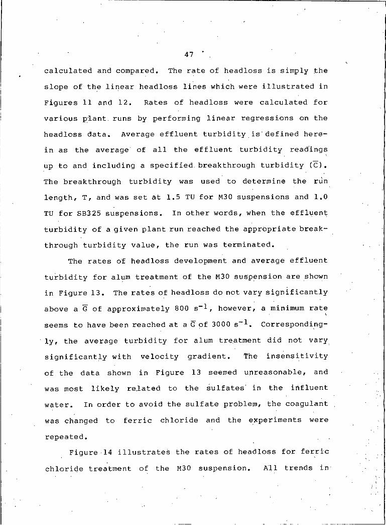
The rates of headloss development and average effluent turbidity for alum treatment of the M30 suspension are shown in Figure 13. The rates of headloss do not vary significantly above a G of approximately 800 s- 1 , however, a minimum rate seems to have been reached at a G of 3000 s- -*-. Corresponding­ly, the average turbidity for alum treatment did not vary significantly with velocity gradient. The insensitivity of the data shown in Figure 13 seemed unreasonable, and was most likely related to the sulfates in the influent water. In order to avoid the sulfate problem, the coagulant was changed to ferric chloride and the experiments were repeated.

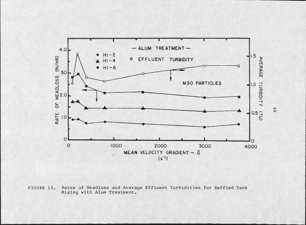
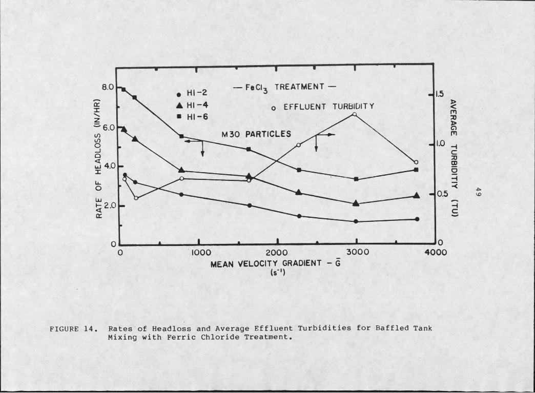
Figure 14 illustrates the rates of headloss for ferric chloride treatment of the M30 suspension. All trends in

RATE

O

F H

EAD

LOSS

(IN

/HR

)

FIGURE

— ALUM TREATMENT —• H I - 2

o EFFLUENT TURBIDITYA H I - 4■ H I - 6

M 30 PARTICLES

IOOO 2000 3000 4 0 0 0MEAN VELOCITY GRADIENT - G

( s ' )

13. Rates of Headloss and Average Effluent Turbidities for Baffled TankMixing with Alum Treatment.

AVER

AG

E TU

RB

IDITY

(TU

)

FIGURE

— FeCU TREATMENT —

▲ H I - 4 EFFLUENT TURBIDITY

M 30 PARTICLES

UJ 4.0

b 2.0

3 0 0 0 4 0 0 01000 2000MEAN VELOCITY GRADIENT - G

( s ' )

14. Rates of Headloss and Average Effluent Turbidities for Baffled TankMixing with Ferric Chloride Treatment.

AVER

AG

E TU

RB

IDITIY

(TU

)

50Figure 14 are similar to the trends for alum treatment; how­ever, note the 100% change in the rate of headless and near 300% change in the average turbidity over the G-value range shown. As a result of the increased sensitivity of the ferric chloride system, no further alum treatment experiments were performed.

The SB325 suspension was also treated with ferric chloride and the resulting headless rates and corresponding turbidities are shown in Figure 15. Once again, the rate of headless changes significantly over the velocity grandient range employed, with high G-values producing lower rates of headless. The average ' effluent turbidities are somewhat less sensitive to changes in mixing for the SB325 suspension in comparison to turbidities for the M30 suspension. The lower sensitivity was actually expected, since on a mass basis (mg/1 ), a finer distribution of colloids will produce higher turbidities (light scattering) than a coarser distri­bution.

It was evident from. Figures 13 through 15, that no clear cut optimum condition could be identified because the head- loss and turbidity data opposed each other. Thus, it became necessary to combine headless and turbidity data into a single filtrability index in order to pinpoint possible optimum mixing conditions. Also, correlations between the turbulent microscale and the colloid distributions could

RA

TE

OF

HEA

DLO

SS (

IN/H

R)

FIGURE

— FeCI3 TREATMENT —

SB 325 PARTICLES

▲ EFFLUENT TURBIDITY■ H I - 6

iO 2000MEAN VELOCITY GRADIENT - G

3 0 0 0 4 0 0 0

(s-')

15. Rates of Headless and Average Effluent Turbidities for Raffled TankMixing with Ferric Chloride Treatment.

AVER

AG

E TU

RB

IDITY

(TU

)

probably not be identified unless a single parameter was used to describe the filter response.

Filtrability Numbers for Baffled Tank MixingFiltrability numbers for various plant runs were calcu­

lated using Equation (9) and plotted against average reactor velocity gradients. .The filtrability numbers obtained are shown in Figures 16 through 18. - Also plotted in Figures 16 through 18 are the turbulent microscales for the impeller stream zone (see Appendix). Figure 16 is for alum treatment of the M30. suspension and the expected insensitivity is evident. Figures 17 and 18, on the other hand, illustrate once again that the ferric chloride system provides much more information in regard to the filter's response to vari­ous degrees of mixing. Since larger filtrability numbers are indicative of poorer filtration conditions, Figures 17 and 18 seem to indicate that relative minimum filtration conditions exist for both the M30 and the SB325 distribu­tions.

Looking back at the grain size distributions for M3Q and SB325, shown in Figure 5, it can be seen that the mean particle size for M30 and SB325 distributions (number count) is approximately 3.0 pm and 6.0 pm respectively. According to the mixing interaction model developed herein, minimum interactions (filtration conditions) should exist when the turbulent microscales are twice the colloid size. Thus,

— ALUM TREATMENT —

M 30 PARTICLES

O 0.75

z 0 .50

H 0 .25

D 2000MEAN VELOCITY GRADIENT - G

3 0 0 0 4 0 00

(s*')

FIGUPF 16. Filtrahility Numbers for Baffled Tank Mixing with Alum Treatment

STREA

M

MIC

RO

SCA

LE (>jm

)

— FeCI, TREATMENT —

M 30 PARTICLES

3 0 .5 0

< 0 .25

2000 3 0 00 4 0 0 0MEAN VELOCITY GRADIENT - G

( s ' )

FIGURF 17. FiltrahiIity Nunhers for Raffled Tank Mixing with Ferric Chloride Treatment.

STREA

M

MIC

RO

SCA

LE (/jm

)

ILTR

AB

ILIT

Y N

UM

BER

xIO

FIGURE

----- FeCI3 TREATMENT -

SB 325 PARTICLES

3 0 0 0 4 0 0 0D 2000MEAN VELOCITY GRADIENT - G

18. Filtrability Numbers for Baffled Tank Mixing with Ferric Chloride Treatment.

STREA

M

MIC

RO

SCA

LE (/jm

)

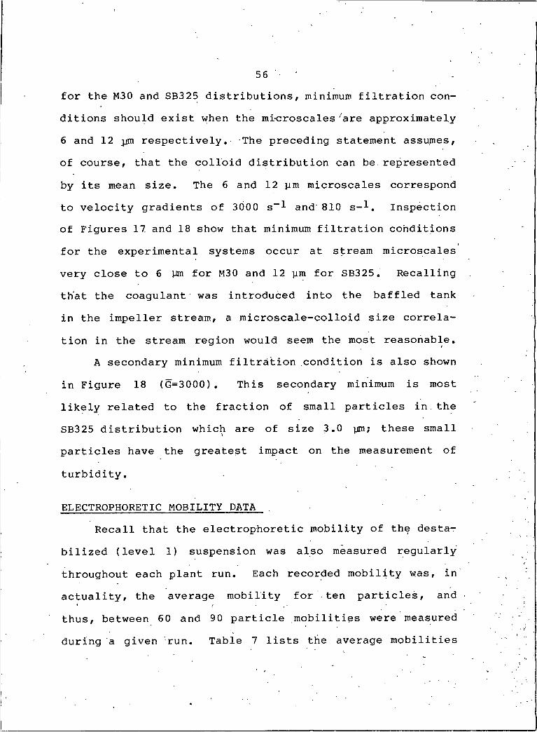
56for the M30 and SB325 distributions, minimum filtration con­ditions should exist when the microscales zare approximately 6 and 12 pm respectively. The preceding statement assumes, of course, that the colloid distribution can be represented by its mean size. The 6 and 12 pm microscales correspond to velocity gradients of 3000 s- -*- and 810 s--*-. Inspection of Figures 17 and 18 show that minimum filtration conditions for the experimental systems occur at stream microscales very close to 6 pm for M30 and 12 pm for SB325. Recalling that the coagulant was introduced into the baffled tank in the impeller stream, a microscale-colloid size correla­tion in the stream region would seem the most reasonable.

A secondary minimum filtration condition is also shown in Figure 18 (G=3000). This secondary minimum is most likely related to the fraction of small particles in the SB325 distribution which are of size 3.0 pm; these small particles have the greatest impact on the measurement of turbidity.

ELECTROPHORETIC MOBILITY DATA .Recall that the electrophoretic mobility of the desta­

bilized (level I) suspension was also measured regularly throughout each plant run. Each recorded mobility was, in actuality, the average mobility for ten particles, and thus, between 60 and 90 particle mobilities were measured during a given run. Table 7 lists the average mobilities

57

obtained from the various mixing conditions employed to treat the M30 and SB325 suspensions. It can be seen from Table 7 that the highest mobilities occur at, or very close to, the microscale-colIoid size correlation points discussed in the previous section. Although the mobility data seems somewhat scattered, any conclusion which is drawn from the mobility measurements is supported by the large number of samples which make up the average values. In fact, statistical analysis of the mobility data yielded

O95% confidence intervals which were so small, that the intervals could be considered insignificant. Thus, boththe mobility data and filtrability numbers seem to sug­gest the existence of a size correlation between the tur­bulent microscale and the mean size of the colloid distri­bution.

HYDRAULIC MIXER COMPARISONSComparing hydraulic mixing to baffled tank mixing was

handled by utilizing the velocity gradient concept. Within the context of this investigation, comparing mixers from a G-value standpoint answered two related questions. First,' the comparisons gave some insight into whether the proposed method for calculating G-values for hydraulic jumps was reasonable. Secondly, comparisons based on G established the jumps mixing effectiveness in relation to the effectiveness

l ' .of the baffled tank. It should be noted here that a similar

58Table 7. Electrophoretic Mobility Data for Treatment

of M30 and SB325 Colloids'

VELOCITY ELECTROPHORETIC*CONDITIONS GRADIENT MOBILITY

(s-1 ) MEAN + 95% C.I.(lim* cm/volt • s)

75 0.90 + 0.02Alum Treatment 210 1.01 + 0.04of M30 Particles 385 1.00 + 0.02

810 0.94 + 0.021640 0.98 + 0.013000 1.15 + 0.033800 ' 1.16 + 0.04

75 1.22 + 0.02Ferric Chloride 210 1.21 + 0.02Treatment of 810 1.09 + 0.01M30 Particles 1640 1.19 + 0.03

2290 1.27 + 0.023000. 1.31 + 0.033800 1.11 + 0.03 ’

210 1.60 + 0.03Ferric Chloride 810 1.52 + 0.04Treatment of 1640 1.70 + 0.02SB325 Particles 3000 1.55 + 0.04

3800 1.44 + 0.03

*Non destabilized particle mobility = 2.2 ym*cm/volt*s

G-value for the jump and tank does not imply a similar Gt value. In fact, for a given G (600—900 S-M the Gt values for the hydraulic jump are an order of magnitude smaller than than the Gt values for the baffled tank.

The rates of headloss of both hydraulic mixers (jump and channel) are shown in Figure 19. The data in Figure 19 indicates that the rates of headloss produced in the filter

-HYDRAULIC JUMP FeCL TREATMENT -

H I- 4JUMPH I- 6

o H I-2 CHANNEL A HI - 4

D H I - 6

3 0 00 40002000MEAN VELOCITY GRADIENT - G

(•-')

FIGURE 19. Rates of Headloss for Hydraulic Jump and Open Channel Mixing with FerricChloride Treatment.

60

for both the jump and the channel are higher than the rates which resulted ,from baffled tank mixing. At first glance, Figure 19 might suggest that the G-values for the jump, were tod large since the hydraulic and mechanical data would align if the jump G-values were less. However, the velocity gra­dient calculation for open channel mixing is well defined, yet the channel data as well, does not align with the baffled tank data.

From a turbidity standpoint, Figure 20 indicates that the hydraulic mixers produced a slightly higher quality effluent than the baffled tank. Thus, the increased head- loss depicted in Figure 19 was understandable.

Combining the headless and turbidity data to form,cor­responding filtrability numbers leads to the comparison il­lustrated in Figure 21. The filtrability data tends to sup­port the G-value calculation method since the baffled tank arid jump data are in good agreement. Furthermore, Figure 21. indicates that the hydraulic jump and open channel are equal­ly as effective as the baffled tank in regard to rapid mixingof chemical coagulants. Once again, it should be noted that

\the actual power dissipations in the hydraulic mixers were .. significantly less than the power dissipations for the baf- fled tank.

AVE

RA

GE

TUR

BID

ITY

(J

TU)

FIGURE

HYDRAULIC JUMP FeCL TREATMENT

• JUMP o CHANNEL --REACTOR

4 0 0 03000O 2000MEAN VELOCITY GRADIENT - G

(#*')

20. Average Effluent Turbidities for Hydraulic Jump and Open Channel Mixingwith Ferric Chloride Treatment.

— HYDRAULIC JUMP FeCl3 TREATMENT —

r O 0.75

CEUJCD23

• JUMP 0 CHANNEL

— — REACTOR

0.50>tCD<CEb 0 .25

/ XZ \Z \Z \

/ \/ \

/ \/ \Z \ZZ \

/

' V -

IOOO 2000 _ 3000MEAN VELOCITY GRADIENT - G

( s ' )

4000

FIGURE 21. Filtrability Numbers for Hydraulic Jump and Open Channel Mixing withFerric Chloride Treatment.

63

CHAPTER I

CONCLUSIONS

Based on the results of this study, the following con­clusions can be. drawn:

1. A size correlation between the turbulent microscale and the colloid distribution seemed to exist for the rapid mixing process of coagulation. The existence of this correlation was supported by pilot plant fil­tration data as well as particle electrophoretic mo­bility data.

2. The microscale-colloid interaction model proposed here­in may provide some insight into the size correlation mentioned above. The mixing model may not actually define the physical nature of the rapid mixing process, however, the model seems to predict the minimum inter­action condition for the mixer used in this study I

3. In regard to optimum mixing conditions, the data col­lected indicates that the size of the colloid suspension being treated must be considered before optimum condi­tions can be defined. The filtr.ability data indicated that average velocity gradients from 700 to 1500 s- l or, possibly gradients above 4000 s~", were best for the

64

particle suspension used in this study.

4. Use of the hydraulic jump design procedure developed here resulted in G-values which were reasonable and functionally correct. Although the procedure developed here was for jumps occurring in sloping channels, a similar methodology could be developed for jumps occur­ring downstream of a critical flow flume.

5. In the average velocity gradient range of 600 to 900s- 1 , the mixing effectiveness of the hydraulic jump was found to be equal to that of the baffled tank. Furthermore, because of the difference in the size of the power dissipation volumes of the jump and the tank, significantly less power was required to produce the above G-values in the hydraulic jump. '

6 . The inflexibility of a hydraulic jump as a mixer was also very apparent. In spite of the attempts made in this study to produce jumps of variable velocity gradient, all the jumps fell within a narrow G-value range. It is this inflexibility that will continue to limit the use of the hydraulic jump in mixing operations.

65

REFERENCES

1. Hinze, J .0. Turbulence. 2nd ed. New YorkzMcGrawHill, 1975.

2. Bradshaw,?. An Introduction to Turbulence and itsMeasurement. New York:Pergamon Press, 1971.

3. Kolmogoroff, A.N. "The Local Structure of Turbulencein Incompressable Viscous Fluid for Very Large Reynolds•Numbers." C.R, Acad. Science U.R.S.S.31

. (1941) : 518.)4. Kolmogoroff, A.N. "On Degeneration of Isotropic Tur­

bulence in an Incompressible Viscous Liquid." C.R. Acad. Science U.R.S.S. 31 (1941):5 38 .

5. Cutter, Louis, A. "Flow and Turbulence in a StirredTank." American Institute of Chemical Engineers Journal 12 (January, 1966) :35-4 5,

6 . Okomoto, Y., Nishikawa, M . and Hashim.oto, K . "EnergyDissipation Rate Distribution and its Effects on Liquid-Liquid Dispersion and Solid-Liquid Mass Transfer." International Chemical Engineering 21 (January 1981):88-94.

7. Camp, T.R. and Stein, P.C. "Velocity Gradients andInternal Work in Fluid Motion." Journal of the Boston Society of Civil Engineers 30 (1943):219-237 .

8 . Leentvaar, J. and Ywema, T.S.J. "Some DimensionlessParameters of Impeller Power in Coagulation-Floc­culation. " Water Research 14 (1.980 ): 135-140 .

9. Chow, V.T. Open Channel Hydraulics. New YorkzMcGrawHill, 1953.

10. Wilson, G .E . "Initial Mixing and Turbulent Floccula­tion" Ph.D. dissertation. University of Cali­fornia, 1972

11. Stenquist, R.J. and Kaufman, W.J. Initial Mixing inCoagulation Processes. U.S. Environmental Pro­tection Agency, EPA-R2-72-053, (1972).

66

12. Amirtharajahf A. and Mills, K.M. "Rapid-Mix Designfor Mechanisms of Alum Coagulation." Journal of the American Water Works Association 74 (April 1982): 210-216.

13. Amirtharajah, A. "Initial Mixing." American Water WorksAssociation, Seminar Proceedings, Coagulation and Filtration: Back to the Basics. St. Louis, MO, 1981.

14. Levy, A.G . and Films, J.W. "The Hydraulic Jump as aMixing Device." Journal of the American Water Works Association 17 (January 1927):1-23.

15. Smoluchowski, M . Physical Chemistry 92 (1917):129.16. Saffman, P.G. and Turner, J.S. "On the Collision of

Drops in Turbulent Clouds." Journal of Fluid Me­chanics 16 (1956):16-30.

17. Spielman, L .A . "Hydrodynamic Aspects of Flocculation"The Scientific Basis of Flocculation (K.J. Ives, editor) Netherlands:Sijthoff and Noordhoff, 1978.

18. Adler, P.M. "Hetrocoagulation in Shear Flow." Journalof Colloid and Interface Science, 83 (September 1981):106-115.

19. Garnet, M.B. and Rademacher, J.M. . "Measuring FilterPerformance." Water Works Engineering 112 (1959): 117-149.

20. CleasbyrJ.L. "Approches to a Filtrability Index fqrGranular Filters." Journal of the American Water Works Association 61 (August 1969):372-381.

21. Ives, K.J. "A New Concept on Filtrability." ' Prog'.Water Technology 10-' (1978) : 123-137.

22. Bisker, C.D. and Young, J.C. "Two-Stage Filtration ofSecondary Effluent." Journal of the Water Pollu­tion Control Federation 69 (February 1977).:319- 351.

23. Lekkas, T.D. "A Modified Filtrability Index for Gran­ular Bed Water Filters." Filtration and Separa­tion 18 (May/June 1981): 214-216.

67

24. • Janssens, J.G., Adam, C . and Buekens, A. "StatisticalAnalysis of Variables Affecting Direct-Filtration" European Federation of Chemical Engineers, Pro­ceedings of the International Symposium on Water Filtration. Antwerp, Belgium:1982.

25. Amirtharajah, A., Personal communication. May 1982.26. Baumann, E .R . Chapter 2 "Granular-Media Deep-Bed

Filtration" Water Treatment Plant Design (R .L .' Sanks, editor) Ann ArbortAnn Arbor Science Pub­

lishers, 1978 .27. Letterman, R.D. and Vanderbrook, S.G. "Effect of

Solution Chemistry on Coagulation with Hydro­lyzed Al(III)!Significance of Sulfate Ion and pH." Water Research 17 (1983): 195-204.

28. Amirtharajah, A. Chapter 28 "Design of Granular-Media Filter Units." Water Treatment Plant De­sign (R.L. Sanks, editor) Ann ArbortAnn Arbor Science Publishers, 1978.

29. Weber, W.J. Physicochemical Process for Water QualityControl. New YorktWiley and Sons, 1972.

«

)

(

68

APPENDIX

SAMPLE CALCULATIONS

i

69Hydraulic jump velocity gradient.

Measurements of depth and elevation within the flume led to the following data for the 1.5 inches per foot slope.

, Ef = 0.078 ft' -y = 0.128 ft"F1 = 3.42 S = sin 6 = 0.124

The power dissipated in the jump can then be found using Equation (7) where

Y = 62.2 Ibs/ft-3 (80°F) 0 = 2.0 gpm = 4.46xl0_3cfs

P = Y Q(Et )

Using F1 , y and S in Figure 22 yields a jump 2

length:L = 0.461 ft

Thus, the dissipation volume, V, is approximated by a triangular wedge of 1.0 inch width or

V = 1/2 Ly 2 (0.0 8 3) ft3

Finally, substitution into equation (2) where y = 1.799x10-3 lb* s/ft3

G = 705 s-1The above G-value being an approximation of the velocity gradient for. the hydraulic jump generated on the 1.5 inches per foot slope.

70

S = 0.25

IOFROUDE **- - F 1

FIGURE 22. Hydraulic Jump Length, L, for Jumps in Sloping Channels.

71

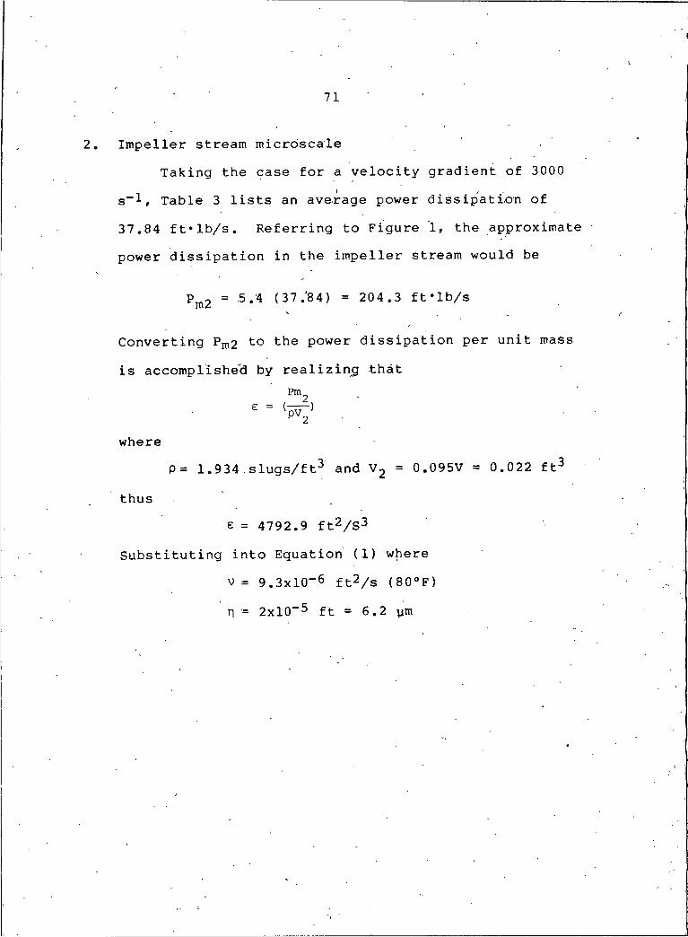
2. Impeller stream microscaleTaking the case for a velocity gradient of 3000

s~l, Table 3 lists an average power dissipation of 37.84 ft'lb/s. Referring to Figure I, the approximate power dissipation in the impeller stream would be

Pm2 = 5.4 (37.84) = 204.3 ft'lb/s

Converting Pm 2 to the power dissipation per unit mass is accomplished by realizing that

whereP= 1.934 .slugs/ft"* and V 2 = 0.095V = 0.022 ft^

thuse = 4792.9 ft2/S3

S u b s t i t u t i n g i n t o E q u a t i o n (I) w h e r e

V = 9.3x10-6 ft2/s (80°F) n = 2x10-5 ft = 6.2 ym

3 1762 00163740

N 378 T776 cop. 2

/ MfTERUBRARY

/(/5#/776