On the equation of turbulent filtration in one- dimensional porous media

Analw. Theo?. Merho& & Appkorrom. k-01 LO. No II. pp. 1303-1325. 1986 0362~546.X 86 33 00 - 00 Prmted m Great B~CNI Pergamon Journals Ltd.

ON THE EQUATION OF TURBULENT FILTRATION IN ONE- DIMENSIONAL POROUS MEDIA

JUAN R. ESTEBAN* and JUAN L. VXZQUEZ’ Divisi6n de Matem6ticas. Universidad AutClnoma de .Madrid, 28049 Madrid, Spain

(Receioed 27 May 1983; receioed for publicarion 21 October 1985)

Key words andphrases: Doubly-nonlinear diffusion equation, turbulent flows in porous media. bounded velocity, finite propagation.

INTRODUCTION AND RESULTS

LET US consider the one-dimensional, turbulent, polytropic flow of a gas in a porous medium. According to Leibenson [20] this flow can be mathematically described by the following equations that relate the density Y, the pressure P and the velocity V of the gas at every point x and time t. First, a polytropic equation of state

P = cy”. (0.1)

Second, the continuity equation

kY, + (YV), = 0. (0.2)

Finally the flux under turbulent conditions is given by

:/v= -MQ,rIQi,/p-r. (0.3)

where the coefficients c, k, M are positive physical constants, the exponents n, p satisfy n 2 1, 4 == p s 1 and @ is related to P by

@ = pk+ 1)/n. (0.4)

Combining the above equations we obtain:

(0.5)

Scaling out the constants in (0.5) we arrive at the nonlinear diffusion equation

(E)

where m = n + 1. The physical considerations imply that u is nonnegative and m 3 2. Never- theless from the mathematical point of view this second condition is irrelevant and we are interested in dealing with all positive m and p. Here we shall study the occurrence of finite velocity of propagation for the solutions of (E). As we shall see later it is necessary in this respect to assume that mp > 1. This condition was first pointed out by Barenblatt [2].

* Both authors partially supported by CAICYT 280583.

1303

1304 J. R. ESTEBAN and J. L. VAZQ~EZ

In this paper we consider the Cauchy problem

(P) 40, x> = uo(x); XER 1

where m and p are positive constants such that mp > 1 and u0 E LL(W) and is nonnegative a.e.

Following the above application we say that u is the density, P = urn-’ is the pressure and the velocity is given by

v= -u,ju,jp-1, (0.6)

with

mP ” = ~ Um-(l/P) - mp _-

mp - 1 mp - 1 p(mp - l).‘ip(m - I))

(0.7)

The equation can be written in the form

u, = (D(u, u,)u,) x.

where the diffusion coefficient

D(u, u,) = mPuP(m-‘) /u,lP-’ = (m - ~)uIu,~P-~

shows that (E) is of parabolic type at the points (t, x) where u(t, x) # 0 and u,(r. X) # 0 but can be either degenerate or singular, according to the values of m and p, if either ~(t, x) = 0 or u,(t, x) = 0.

In the case of laminar filtration, p = 1 (cf. [20]), we obtain the equation

ut = (u”),, I

usually known as the porous media equation if m > 1, or the fast diffusion equation if 0 < m < 1. If m = 1 we have the linear heat equation. All of them have been widely studied in the literature, cf. [l, 21, 22, 261.

The case m = 1, p # 1 appears for instance in the study of non-Newtonian fluids. cf. [13] and its references.

The general case m # 1, p # 1 has been studied by several authors. Those contributions related to our work will be commented upon later.

*We next state our main results. First, using the dissipative character of the operator

in the space f.‘(R) of the Lebesgue-integrable functions in --x < x < +x, we show the existence and uniqueness of a strong solution of(P):

THEOREM 1. Under the stated assumptions on uo, m and p there exists a unique function

u E C([O, =); L’(R)) r-l L”([6, =) x W) /f’6>0

On the equation of turbulent filtration in one-dimensional porous media 1305

satisfying:

(a) u(O,x) = Us a.e. x;

(b) a.e. t > 0 Urn(f, .) E w’.X(lR);

Moreover,

I II t, x ,~“,) ‘f ( )? (?,) 1.2 ; Y are the solutions corresponding to initial data Us, co(x) then for every

j+‘ [~(t, x) - ic(t, x)1+ dr s j+x [uO(x) - fi,(x)]+ dr. (0.8) --x -2

In particular, llo s fro a.e. implies that

u(t, x) S qt, X) a.e. x (0.9)

for all t 2 0.

(e) Smoothing ejfecr. For every r > 0, x E R we have

]@, ,r)] < C(m, p)t-L’(“(“+‘))lll(O(ljP+l)i(p(m+l)) (0.10)

and the best constant C(m,p) > 0 corresponds to Barenblatt’s solutions [2] (see the explicit values in (1.36)).

(f) If ~1~ E L’(R) n L”(R), then for every t > 0, x E W

k(‘? XII =s I/4. (0.11)

The construction of a solution of (P) is done for every ~1~ E L’(R) and positive m, p. In proving that u is a strong solution if u. 2 0 and mp # 1 we use results of Benilan [3, 41. For the smoothing effect we follow [24].

Our main result consists in showing that the velocity V(t, x) associated with this solution is a bounded function of x and t for t 2 t > 0 even if the initial velocity function is unbounded, From this property the Holder continuity of the solutions follows.

THEOREM 2. If ~(f, x) is the strong solution of (P) with u. E L*(R) n L”(W), llo 5 0 a.e. m,p > 0, mp > 1, and if V(t,x), o(t, x) are as in (0.6), (0.7) then

(a) for every t > 0, x E W

]V(t,x)] = ]/J&X)]P G Ct-PI(P+I)IIUOJI~mP-l)‘(p+l) (0.12)

for some constant C = C(m,p) > 0.

(b) In every strip S, = [t, xc> x R u is Holder continuous in t and x with exponents y/(y + 1) and y respectively,

1306 J. R. ESTEBAS and J. L. VAZQL-EZ

and coefficient C = C(s. m,p, jlu&). Note that, because of (O.lO), there is no real loss of generality in assuming that u0 is bounded. When p = 1 this result was proved by Aronson [l]. The corresponding result for m = 1 was

subsequently proved by Herrero and one of the authors [13]. A related result for general p and m was obtained by Kalashnikov [14]; for continuous. nonnegative and bounded initial data u0 such that u~-(‘!P) is Lipschitz-continuous (i.e. the initial velocity is bounded) a generalized solution having bounded velocity is constructed in [14], using the fact that by the maximum principle the bound for the velocity is preserved in time. The uniqueness question for this class of solutions remains open.

The condition mp > 1 is necessary. Actually, in one of the first mathematical contributions to this problem, Barenblatt [2] constructed a class of explicit self-similar solutions corresponding to initial data a Dirac mass. These solutions have bounded velocity and compact support in x for every t > 0 if and only if mp > 1. In our case mp > 1 these solutions read

where

iS(r, x; M) = t- li(p(m-i)){C _ k( , m p)(i,+-! (P~m-l)))(P+l)iP}P:“(mp-‘)) (0.13)

k(m,p) = myi: i)ip(m’+ 1))“”

and C is computed in terms of M from the equation

i

+ X IM = Z(f, x; M) dX for any t > 0. (0.14)

--z

The importance of the Barenblatt solutions lies on the fact that they will seme as a model for the propagation and asymptotics of all the nonnegative solutions of (P) with u,) E L’(R), in particular if u0 has compact support. In the case p = 1 many results in this direction have been proved, cf. [12, 16, 221. If m = 1, cf. [13].

In particular the velocity for the solutions (0.13) is given by the simple formula

x

V(r, x; M) =

i

P(m + l)t if js G r(t),

(0.15)

0 otherwise,

where

r(t) = c(m,p)M (mp-l)l(p(m+l)lfl.(p(mtl)) (0.16)

(Observe that 1x1 < r(t) is the region where G(t,x; M) > 0.) Combining the smoothing effect (0.10) in the interval (0, t/2) with the velocity estimate in (t/2, t) we obtain

COROLLARY 1. Let mp > 1. For every 1(0 E L’(R), u0 2 0 we have

]v(f,x)] s Cf-(p(m+l)-l)l(p(m+l)) /]L~O]]~-‘)~(p(m+‘))

for some C = (m,p) > 0.

(0.17)


This is precisely the result that follows for V(r, x; M) from (0.15). (0.16). In other respects, since the function V(r, x; M) is discontinuous in jxl = r(r). the regularity

u E C’! with respect to x in theorem 2 is sharp. The property of bounded velocity implies that the support of the solution propagates with

finite speed. It gives rise to the appearance of curves, called inferfaces or free boundaries, that separate the regions where u(r, x) > 0 and where rt(t, x) is zero. This fact and its consequences are well known in cases p = 1 or m = 1. We devote the last section of this paper to show how the above results can be used to prove that the interfaces are Lipschitz-continuous, nondecreasing curves (theorem 4).

Other results about propagation properties of the solutions of equation (E) can be found in [15] which also contains references to related literature.

The rest of the paper is organized as follows: In Section 1 ae prove theorem 1. Section 2 deals with the solution of a Cauchy-Neumann problem necessary as an approximation for the proof of theorem 2, which is done in Section 3. In Section 4 we study the interfaces.

SECTION 1

This section is devoted to the proof of theorem 1. In a first step we use the nonlinear semigroup theory to construct a generalized solution of the evolution problem

(1.l.a)

LL(O,X) = uo(.u) E L’(W). (1.l.b)

This solution, usually called mild solution, satisfies u E C([O, x); L’(W)). u(O) = 1~~. In step 2 we show that this solution is in fact a strong solution of (1.1) and in particular

satisfies (b) and (c). The uniqueness, (d) and (f) are treated in step 3. Finally, in step 4 we prove the smoothing

effect.

Step 1. If we have a (possibly multivalued and nonlinear) operator A in a Banach space X with domain D(A) C X the semigroup generation theorem (cf. [lo, 111) says that we can construct a solution u E C([O, T]; X), T > 0, of the abstract evolution problem

K, -+ A(u) = 0

U(0) = Ug I (1.2)

if ug E D(A), the closure of D(A) in X, and A satisfies:

(i) For every U, fi E D(A) and every A > 0

I/U - fi]lx s ]](u + ,lAu) - (fi + /lAri)llx (1.3)

where 1). jIx is the norm in X. We say then that A is accretiue and also that -A is dissipatioe.

(ii) Range condition. Range (I + J.A) = X for every (or equivalently for some) J. > 0.

An accretive (resp. dissipative operator satisfying the range condition (ii) is called m- accretive (resp. m-dissipative).

1308 J. R. ESTEBAN and J. L. V.AZQCEZ

To obtain the solution of (1.2) we have to associate to every finite partition

a={r,=O<t,<...<t,~T}

of the interval [0, T] an approximate solution 11“ of (1.2) by means of discretization in time: u“ is a step function of the form

uO(r) = up ift, <t< tk+l (1.4)

and the {u:}~ are defined recursively by the implicit scheme

u; = 110 ( (l.S.a)

u;+, - Ll;

fk+l - tk

+ A(u$+~) = 0. (1.5.b)

Then the solution u is obtained as the uniform limit (in C([O, T]; X)) of the family {[IO(~)} as the diameter of u tends to 0. The unique function thus obtained is usually called the mild solution of (1.2) and the maps {S, : [lo - u(t)}, form a continuous semigroup of contractions in X, cf. the survey paper [ll] for other results.

Problem (1.1) can be cast in the form (1.2) by delinin, 0 the nonlinear operator A in X = L’(R) by

A(rl) = _ -t(%k$!&“), (1.6)

where G(r) = r/$“-I, in the domain

D(A) = {U E L’(R) : @(IL) E W’~x(W), A(u) E L’(Iw)}. (1.7)

The fact that A is m-accretive in L’(R) is a consequence of the following result: let us write u + A(u) = f in the form

-(u’Iu’Ip-1)’ +‘p(u) =f (1.8)

with u = G(u) and P(I) = 4-l(r) = ~lrj(~‘~)-l. We have:

PROPOSITION 1.1. For every fE L’(R) there exists a unique u E W’*x(W) such that u = p(u) E D(A) and (1.8) holds a.e. Also u(x) and u’(x)--, 0 as /xl+ x.

IffE L”(R) then 14 E L”(W) and a.e. in iR

-Ilf-II= s 4x> s IlfflL~ (1.9)

Moreover if D is the solution of (1.8) corresponding to another second member f and ic = /3(G) we have

IKU - @+lll c llw--ml f (1.10)

where s+ = max(0, s}, s- = max(0, -3).

Remarks. (1) (1.10) implies at the same time that A is accretive and that the maximum principle holds, i.e. iffGfa.e. then u s fi and u s 0 a.e. Property (1.9) is usually called T-accreriuity of A in L’(R). This concept generalizes in an obvious way to other spaces [Lp(W), 1 Sp S X, cf. [18].


(2) We shall prove the proposition in the more general situation where C#J = p-r is any strictly increasing continuous function R ---, W such that Q(O) = 0 (in fact we could even consider discontinuous 4’s as in [5] where @ is a maximal monotone graph in ‘R).

(3) In case p = 1 this proposition is theorem 4.1 in [j]. Actually our proof consists in following basically their argument and using results of [18] to deal with the nonlinear principal term.

Proof of proposirion 1.1. It is well-known, cf. [13]. that the p-Laplacian operator B(u) = -(u’lu’]P-‘)’ with domain

D(B) = {Ld E L’(R) : u’ E C(R), B(u) E L1(R)}

is m-accretive in L’(R) and T-accretive in L”(R). Using theorem III. 1.1 of [18]. we deduce that /I + B is m-accretive in L’(R) and T-accretive in L”(R) with domain D(B) n {u E L’(W) : /3(u) E L’(R)}. Therefore, for every E > 0 we obtain a solution u, E D(p + B) of

EU, + ,D(o,) - (o:]o:]q’ = f. (1.11)

Now for fixed E > 0 we have (u;]r~:]P-~)’ = EU, + p(u,) -f E L’(R), therefore the function u:]u:]p-’ is continuous and admits a limit as x-+ m and as x--, -2. If, say, the limit as x+ x is not 0 then it is easy to see that Ju,J ---, = as x - = contradicting the fact that p(u,) E L’(W). Hence

ijmlz u:]u:]p-i = 0. (1.12)

From this and p(u,) E L’(W) it follows also that

lim u,(x) = 0. lxl*x

(1.13)

Now we can multiply (1.11) by a smooth approximation of the sign0 function. sign&r) = sign(r) if r # 0, =0 if r = 0, to obtain by standard integration by parts

+CIli + llP(uc>ll~ s jixfsienO(u,) s llfllly (1.14) --x

hence ]]/3(u,)]i, s Ilflll. Integrating (u:]u:/P-‘)’ between --r; and x and using (l.ll), (1.12), (1.14) gives

IuXx)P s 2llflL. (1.15) On the other hand if we set j(r) = JLp(s)dr then j(u,)’ = /3(u,)u: E L’(R). As before the

limits of j(u&)) as x --, x and x + --x exist and they are 0 since p(u,) E L’(Z). Finally integrating j(u,)’ = p(u,)u: gives

Ili(~,)llx G II4 lIP(UE s 21~llfll’p+1)‘p. (1.16)

Now by the assumptions on /?, j(r) + = as ]r] --, =, therefore (1.16) implies that {u,}, is a bounded family in L”(W) and, by (1.15), in W’-x(W).

Now let E--* 0 in (1.11). Then u, -+ u uniformly on compacts, hence p(u,) ---* B(u) in the same way; EU,+ 0 uniformly on R. We see then that u E W1.x(R), /3(u) E L’(X). u satisfies (1.8) and the estimates (1.15), (1.16) and ]]p(u)]ll G ]]fl]i. To prove that u, u’-+ 0 as .r/ + x: we can repeat the above argument.

1310 J. R. ESTEBAS and J. L. VAZQUEZ

The proof of (1.10) follows a standard argument: we substract the equations for u and 6, multiply by a smooth approximation of (sign,,(u - 6)) +, integrate in Fa and use the accretivity of B in L’(R):

I += (B(u) - B(fi))(sign,(o - 0))’ dr 2 0. (1.17)

-?z

PROPOSITION 1.2. D(A) is dense in L’(W).

Proof. It is enough to prove that D(A) 3 L’(L’Q) n L”(Iw). Since A is m-accretive in ,5,‘(Oa) (proposition 1.1) for given f E L t(W) n Lz( W) and A > 0 there exists a unique ~1~ E D(A) satisfying

-A(U;]U;]P-‘)’ + K;, =f, ui = @(KA). (1.18)

we want A + 0. the of [6,

j’ (K-f) (1.19) -z --r

uniformly in R. Finally since A]u~(x)]~ s 2]]f]] I (cf. (1.15)) (p assing to a subsequence) we have

AllPu' A + w in Lx-weak*. (1.20)

Necessarily w = 0. (1.19) and (1.20) imply that 0 = ,:,(K -f>, hence u =f a.e.

Remark. The above results are valid under the assumption 0 < m, 0 < p with no restriction on the sign off or II.

Step 2. Here we prove that the mild solution obtained in the previous step is a strong solution

of (1.1) if mp > 1 and u. 2 0. By this we mean that 14(t) is absolutely continuous from [0, m) into I,‘@), and for a.e. t > 0 u is differentiable into L’(W), u(f) E D(A) and (1.1) holds.

By [ll, regularity theorem (iii)], it suffices to show that a.e. in (0, m) K is differentiable into L’(R). This can be done using the ideas of [3, 41 as follows.

PROPOSITION 1.3. Let K be the mild solution of (1.1) with u. E L’(W) n L”(R), u. 3 0 a.e. and mp > 1. Then u is differentiable into L’(R), a.e. in (0, z).

Moreover TV, E L"(0, 3~; L’(W)) and

fb‘rll I c & lb~ll~ , (v - l)tu, 2 -u a.e.

and we have

t](K (m+1)‘2),]Z dx dt < cjlKOll;=;

(1.21)

(1.22)


(1.23)

ifO<m<l.

Remarks. (1) As we will see independently in step 4, there is no restriction in assuming 110 E L”(W).

(2) Proposition 1.3 is also valid in case 0 < mp < 1 with similar proof. This is not true if mp= 1.

Proof ofproposition 1.3. (i) We first give a proof of (1.22) following the formal calculations of [3]. We take partitions of fixed step E > 0 in the scheme (1.5). Hence rk = k& for every k = 1,2, . . Then (1.4), (1.5) read

u,(r) = u; if k& s t < (k + l)~, (1.24d)

uo’ = 110,

u; - A(u&) = 0; k= 1.2.. . .

E 1

> (1.24b)

Since 11 ,, 2 0, by (1.10) we have u,(r) 2 0. We set u,(t, x) = n,(f. x)” and

WE(f, x) = f (Il,(f, X)(m+1)/2 - U,(f - &,X)(m+r)!?}.

Then elementary inequalities give

(1.25)

(1.26)

Using (1.23) we replace the last factor by -A(u;). Since u,(t), ~,(t - E) E D(A) if 2~ < t we can integrate by parts and get

’ I_ ax ax I

~ k&‘1’, j+x [ i”“;yp+’ -I

Now we define the functions

5;,(t) = [;k _ 2) iftC2E

& if (k - 1)~ s t < k&,

- dr. (1.27)

k=3,4,...

1312 J. R. ESTEBAN and J. L. V.AZQKEZ

bfultiplication of (1.27) by cE(r) and integration in t give, for n = 2.3, .

nE

i j CE(f) +X lw,12 drdt = i jkE

-x k=3 [k-1)E

cE(f) j+X jw,ll drdr --x

On the other hand, if 13 E, we have again u,(~.x) - I(,([ - E,X) = -&A(~,(f.x)). hence multiplying by u,(t. x) and integrating by parts we get:

+x {u,(t - E. ,K)~~’ - u,(t, x)“‘+‘} dv

and then II- 1

TX au,(kE.x) p-l &

=i I ax I&)~+~ du.

k=2 --r

Therefore, letting n -+ x we have obtained that

io+x I +x m+l +=

CE(f) I

LQ(x)m+’ dx. --x

Iw,(r, ,~)I? dx dt =s qp + 1) _-x (1.28)

In the case 0 < m < 1 we can obtain by a similar line of argument the estimate

see the details in [4] where the case of a bounded domain is treated. In the limit as E+ 0 we obtain (1.22), (1.23). (ii) Now we use the fact that A is an homogeneous m-accretive operator, i.e. A(l.rc) =

,i”‘pA(~) for every A > 0, u E D(A), to deduce from [7] that

t += u(t + h, x) - ~(t, x)’ I I h -cc

(1.30)

for h > 0. In case 0 < m < 1 this means, together with (1.23) that tj~,j E L”(0, “; L’(X)) and u is a.e. differentiable into L’(R) (see [8, Appendix]). In case 1 G m it follows from (1.22) and [3, lemma 41, that the function u(t, x) = t~(f~p-‘, X) satisfies

u E W;c’(O, =; L;,,(W)


for every r, 1 6 r < 1 + (l/m). Then (1.30) implies again that rju,j E L”(0, X; L’(g)) and u is a.e. differentiable into L’( $3).

The second part of (1.21) is now a consequence of [7].

Step 3. We can prove property (d) of the theorem 1 in a standard way by multiplying the equation by a suitable approximation of sign<(u” - rim) and integrating by parts. But the result can be also derived as a consequence of its elliptic counterpart (1.10). In fact it is easy to see that the mild solutions satisfy (d) because of (1.10) and the discretization process. Now the solutions of theorem 1 being strong (properties (a)-(c)), they are mild (cf. [9]). Property (f) follows in a similar way.

Step 4. Smoorhing effect. We show the following result. valid for m,p > 0, u. E L’(2).

PROPOSITION 1.4. Let u be the mild solution of (1.1) with llr, E L’(R). Then for every t > 0 u(t, x) is a bounded function of x and

(1.31)

where C = C(m,p) is a positive constant. The best constant C(m,p) is attained by the Barenblatt solution [2].

Proof of proposition 1.4. It is based on a comparison result that uses the technique of Schwartz symmetrization as follows: For any function fE L’(W), n 2 1, we define the symmetric decreasing rearrangement off as the function f’ such that

f”(x) = inf{s : meas{/f(x)] > 5) s CJX]“}, (1.32)

where C, = &‘/T(l + (n/2)) is the measure of the unit ball. f” is nonnegative. radially symmetric and integrable.

Now we consider the problem (1.1) with data u. and ri, E L’(W) such that:

(1) I&, is radially symmetric and decreasing; (2) for every r > 0 we have

(1.33)

Then if U, Li are the respective solutions of (1.1) we have:

(1’) for every t > 0, ti(t, . ) is radially symmetric and decreasing; (2’) for every t > 0 and r > 0 we have

i U*(t, x) dx s

i ic(r, x) dx (1.34)

ix’<r IX/ST

where ~*(t, x) means the rearrangement with respect to x variable with t fixed. In particular (1.34) implies that

LP(t, 0) = sup]u(t, x)] s il(t, 0) = sup cqt, x). (1.35) x I

The results (1’) and (2’) are proved in [24] in the case p = 1 (but in dimensions n 2 1) and the proof applies to our case without changes. In case p # 1, m = 1, see [25].

1311 J. R. ESTEBAN and J. L. V.AZQCEZ

We now want to compare the solution u with the Barenblatt solution 17(r, x: ,Cf) = ri to obtain (1.31). This poses the problem that 1T(O, X; iU) = ,CIS(x) is not an integrable function. Therefore we proceed as follows.

Let first u be a solution with 110 E L’(A) n L=(A). Then fi(t. X) = ti(r + 7. I; .CI). -If. T > 0 is a strong solution of (l.l)-as can be easily checked-such that il, satisfies (1). (3) above if r

is small enough and M = E + /lrlO//r with E > 0, E+ 0 as t-+ 0. Therefore (1.35) implies that

~n(t,x)l s Lqt + t, 0, AZ) = C(m,p):WP-” (p(m+‘))(f + r)-l (Hrn-‘)’

S C(m, p);LI (PTl) (p(m-l))t-l,(p(m-l)).

Letting t+ 0 we obtain (1.31). For general LL the result follows by approximation (use theorem l(d)). Computation of the constant C(m,p) in the Barenblatt solutions gives the explicit values

case mp > 1

(p+ lV(p(m+ 1))

(1.36a)

case 0 < mp < 1

C(m,p) =[,(,‘_ l)(p+)P+‘(~(~ ~~))p]“iP’m+‘ll

(p+l)l(p(m+l))

(1.36b)

case mp = 1

C(p) = (p’p-‘)l(p+‘))/{2r(p/(p + l))},

where T denotes the Euler gamma function.

SECTION 2

This section deals with the solution of the Cauchy-Neumann problem

a a - ur - x v g Q(u) ! ) forO<x<l, O<r,

1 u(O,x) = 4l(x) forO<x< 1,

v(kf$(~(l,x))) =0 forx=O, x=1, O<r, i

(2.1)


where

$ : W - W is a strictly increasing. continuous function, 0 = G(O), (2.2)

t+ : R -+ W is continuous. nondecreasing, 0 = ~(0) and !1_” iv(r)1 = x. (2.3)

Although a much more exhaustive treatment of (2.1) is possible. we will restrict our attention just to the facts we will need in the proof of theorem 2. As in the case of the Cauchy problem, the semigroup generation theorem provides the mild solution of (2.1): the arguments being analogous to the ones used in the proof of proposition 1.1, they rely on the following two facts.

(i) The m-accretivity in L’(0, 1) and T-accretivity in L”(0. 1) of the operator

with domain

D(A) = [Ld E L’(O, 1) : q(u) E wyo, 1). q-$@(U)) E W$i(O. 1)).

(ii) Theorem 111.1.1 in [18].

In Section 3 the point of interest on (2.1) will be the continuous dependence on I+U of the mild solutions of (2.1). For llo E L’(0. 1) fixed and for given y, y,, (n = 1.2. . . .) satisfying (2.3) we consider

the mild solution of

Ll,l E C([O, T]; L’(O.1))

u n.l =;Y”(-$(LL)): O<X<l, O<t

LL,(O, x) = u,(x): o<x< 1, I

Yn (A 4(Lln(f. -4) = 0; x=0, x=1, 0 < t, J

and u the mild solution of (2.1). We have the following result

PROPOSTION 2.1. Let v, I/J,, satisfy (2.3) and

v,, - r~ uniformly on compact subsets of R.

I Y, (4 -+ r as 14 + x uniformly in n.

Then

U, --, u in C([O, T]; L’(0, l)), T> 0.

(2.4)

(2.5)

(24

(2.7)

1316 J. R. ESTEB.AS and J. L. V.AZQLEZ

Proof of proposition 2.1. We set

and for every

n= 1,2,. . . An = - ; vjl, c ) g @(u>

From the perturbation theorem of nonlinear semigroup theory (cf. [ll]), (2.7) follows if A,-+ A as m-accretive operators (i.e. in the resolvent sense). Thus for any givenfE L1(O, l), if IL, E D(A,) solves u,, + A(u,) = f and u E D(A) solves u + A(u) =fwe have to prove that u,- u in L'(0, 1).

Setting p = p-i, U, = p(u,), u = p(u); this means that if

and if

a.e. in (0, 1)

0, E W’,‘(O, l), w,(uA) E Wb,‘(O, l), P(u,) E L’(O, 1) I

(2.8)

P(u) - $ v(u’) =f a.e. in (0, 1) (2.9)

u E Wi.‘(O, l), 7#(u’) E Wh’(O, l), P(u) E L’(O, l), J

we have to prove that

P(rJ!I) ---, P(u) in L’(0, l), asn-+x. (2.10)

Now it follows from (2.8) that ]/p(u,,)]]i G ]]f]]i and ]]r/~,,(uA)]]~ G 2]]f]/i. From (2.6) we get that ]]uA]], G C < = for some C > 0 which is independent of n. To prove that {u,}, is a bounded

sequence in L”(0, 1) we may argue as follows: if {u,} were not uniformly bounded then

]]u~]], G C would imply that for every k = 1,2, . . . we could find nk such that k s u.,(x)l for

all 0 c x c 1, and this contradicts ]]p(u,)]]r =Z ]]f]],. Therefore {u,} is bounded in IV’~“(O. 1) and (passing to a subsequence) u, ---, u uniformly on [0, 11, and likewise p(u,,) --+ p(u). The fact that u and p(u) satisfy (2.9) follows easily as in proposition 1.1.

SECTION 3

In this section we prove theorem 2. In order to estimate ]u,(t,x)], the basic tool will be

Bernstein’s method applied to the equation satisfied by u. Formally this equation reads

u, = (rnp - l)u]u,]p-iv, + ]u,]p+i. (3.1)

Nevertheless, because of the degeneracy of this equation when u = 0 or when I,, = 0, we cannot work directly with the solutions of (3.1). We will obtain smooth approsimations of u(t, x) by taking strictly positive, smooth initial data and by smoothing the nonlinear function r/~(s) = s]s~J’-’ which acts on (u~)~. Thus Bernstein’s method is applied to the smooth solutions


of these approximate problems, and this is carried out not for the Cauchy problem but for the Cauchy-Neumann problem, because the main lemma (lemma 3.3) deals with functions uO(x) 2 6 > 0 that would not be integrable in the whole line. Finally, we use the continuous dependence result proved in proposition 2.1 to recuperate the strong solution obtained in theorem 1.

These difficulties can be considerably circumvented if p = 1, cf. [I], or if m = 1, cf. [13], because we can work directly on the positive solutions of (3.1). For p = 1 these solutions are classical. For m = 1 we can use the fact that the operator B(u) = -(u’]u’IP-‘)’ is m-accretive in every space P(W), 1 S p < x, to prove first that they are classical except where u, = 0.

We begin with the construction of the smooth approximations ~~(5) of the nonlinearity t/~(s) = s~s]P-~, where p > 0.

LEMMA 3.1. For every E > 0 there exists a Cx(R) function qE(r) satisfying:

l&,(r) = v(r) = rlrlp-’ if c S ]r(;

There exists Cr (p), Cz (p) > 0 such that for Irl S E : C,(p)EP-* C v;(r) S C&)Ep-‘.

(3.2)

(3.3)

Proof. Consider the following cut-off function

p(r) = i

Ce'P[+2)

0

with a constant C > 0 such that Jp(r)dr = 1. Now let

<0(r) = @[l -i/E;2 P(1 +

if Iri < 1

if /r/ 5 1

i (s - 9) dq

and

We can define WE(r) E Cx(W) as v,(r) = A&(r) + cl(r)+ if 0 G r, WE(r) = - vE( -r) if r < 0. If I. = A(p) > 0 is suitably chosen when vE satisfies (3.2), (3.3).

LEMMA 3.2. Let r+, E C;(-R, R), u. L 0 and let E, 6, R be positive constants. The Cauchy-

Neumann problem in Qr,a = (0, T] x (-R, R): 3

a UC = G vc O<t, IX/CR,

u(0, x) = 6 + uo(x); 1x1 s R, (3.4)

+$I, *R)) =O; Ott

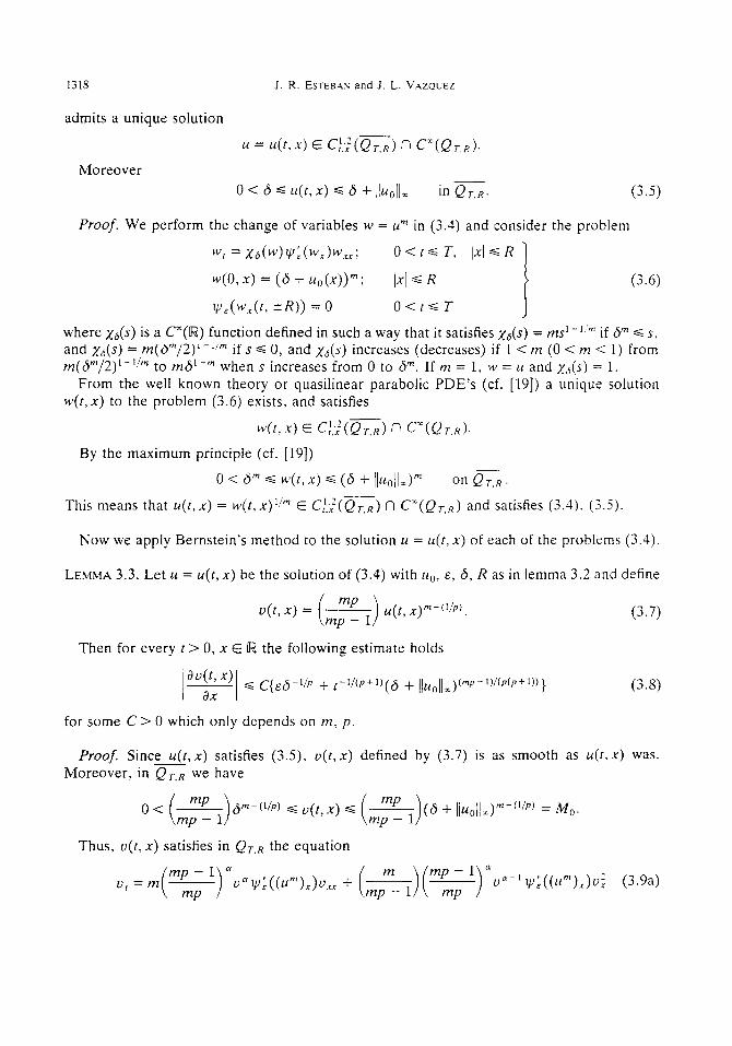
1318 J. R. ESTEBAS and J. L. V.AZQUEZ

admits a unique solution

u = ~(t,,r) E C,iYQ,.,, n CX(Qr.~).

Moreover

Proof. We perform the change of variables w = llrn m (3.4) and consider the problem

wr = %6(~)w:(wr)~,; O< to T, Ix/ s R

w(0, x) = (6 + u&))“; 1x1 c R

1

(3.6)

~jl~(\vx(r. -R)) = 0 O<tsT

where x6(s) is a CX(R) function defined in such a way that it satisfies x6(s) = rns’-I’“’ if 6” G s, and x6(s) = rn(~Y/_))‘-‘~~ if s G 0, and x6(s) increases (decreases) if 1 < m (0 < m < 1) from @m/2)‘+ to ma’-“’ when s increases from 0 to 6”. If m = 1, w = 11 and x6(s) = 1.

From the well known theory or quasilinear parabolic PDE’s (cf. [19]) a unique solution w(t,x) to the problem (3.6) exists, and satisfies

w(t,x) E ~:;‘(QT.R) II Cx(Qr.~).

By the maximum principle (cf. [19])

0 < 6” s w(t, x) G (6 + ]jUal],)m on QT.R. This means that u(r,x) = w(t,x) Urn E C::“(G) n CX(Qr,R) and satisfies (3.4). (3.5). .

Now we apply Bernstein’s method to the solution u = u(t, x) of each of the problems (3.4).

LEMMA 3.3. Let u = u(t, x) be the solution of (3.4) with u”, E, 6, R as in lemma 3.2 and define

mP u(t, x) = ~ ( i u(t, x) m-U/p) mp - 1

Then for every t > 0, x E Iw the following estimate holds

au(r, x> 1 i s C{&i/P + t-MP+U((j + IJu”llr)(mp-‘)i(p(p+‘))} 8X

(3.7)

(3.8)

for some C > 0 which only depends on m, p.

Proof. Since u(t, x) satisfies (3..5), u(t,x) defined by (3.7) is as smooth as n(r. X) was. Moreover, in Qr,R we have

o< -_!E!L ( ) mp - 1 Bm-(‘/p) 6 /J(t, x) =s ( ) = (6 + lluollf)“-(“p) = M,,.

mp - 1

Thus, u(t, x) satisfies in Qr,R the equation

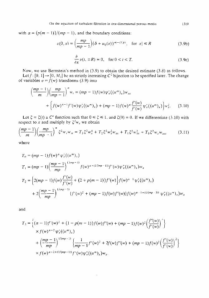
On the equstlon of turbulent filtration in one-dimensional porous media 1319

with 1y = (;3(m - l))/(mp - l), and the boundary conditions:

u(0. x) = (6 + ~,,(,~))~-(ip), for l,rj s R (3.9b)

$ u(t, rR) = 0, forO<r<T. (3.9c)

Now, we use Bernstein’s method in (3.9) to obtain the desired estimate (3.8) as follows. Let f: [0, l] + [0, MO] b e an strictly increasing C’ bijection to be specified later. The change

of variables u =f(~) transforms (3.9) into

(C)($!J wr = (“P - I)f(~,)v,;((U”‘).r)W,.~

+ f(w)“-If’(W)~CI:.((L(“),~) + (mp - l)f(W)“f”(w) I f’o V:(W).&. (3.10)

Let c = c(t) a c” function such that 0 S c G 1, and c(O) = 0. If we differentiate (3.10) with respect to x and multiply by c%v, we obtain

(e)(s)” [‘~,w,~ = TjC’wi + TrfZ~z~,,,r + T,~?w,,~ + To<?w.,~,, (3.11)

where

To = - l)f(w)“v-‘;((~~“)r)

f(w) n+(“(mp-‘))f’(W)1CI’:((Um).~)W,

T2 = f”(w)

2(mp - l)f (w) f ,(w) - + (2 + p(m - l))f ‘(w)}f(w)a-l vi((L~“)~)

+2 mp _ 1 b+v-l)

i 1 mp {f’(w)’ + (mp - l)f(w)f”(w)}f(w)R.-‘t(l’(m~-‘)) yI;((llm),c)bv,

and

(N - l)f’(w)’ + (1 + p( m - l))f(w)f”(w) + (mp - l)f(w)‘(;$$)‘}

x f (WY V,:((~~“).r)

+ (m;; l)‘i’mp-” [ &f ‘(WY + 2f (w)f”(w) + ( mp - l)f(w)?(;z

xf(w) ~-2+(ev Wf ‘(w)~u’;((LqJw,.

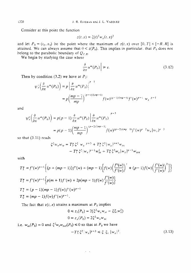
120 J. R. ESTEB.AN and J. L. V.AZQLEZ

Consider at this point the function

Z(f.X) = qf)GV,(f, x)’

and let PO = (to, x0) be the point where the maximum of z(t. x) over [0, 7-1 x [-R. R] is attained. We can always assume that 0 < z(P,). This implies in particular, that P,, does not belong to the parabolic boundary of Or,,.

We begin by studying the case where

i a (G u”(P,) z= E. (3.12)

Then by condition (3.2) we have at P,:

mp - 1

i ) (p- IhYv- II

= P- mP

f(,)(P-l)i(WlI f’(w)qw,JP-

and

I$,($ u”‘(P,)) = p(p - 1) $ Urn(PO) 1 $P(zJ()) iy+

mp - 1 (P-NV-l)

=p(p-l) ~ i 1 mP

f(W)(p-3)!(mp-l)f’(W)P-2W,I,~,~~-i

so that (3.11) reads

<‘LV, WC1 = Tj” i? / it*., 1 Pi-j + T; i” 1 IV, lP+‘w,,

+ TT ;2/w,Ip-1 w:.r + T,* C’w, 1 wx ip - ’ wx,

with

TT = f’(~>~-~ ((P + (mp - W”(w) + (mp - 1) [f W( ;$$$) ’ + (P- W(W) (;$$) *I} T,C = f’(w)J’-‘[p(m + l)f’(w) + 2p(mp - l)f(w) iz]

T,’ = (p - l)(mp - l)f(w)f’(w)P-I

T,* = (mp - l)f(w)f’(w)P-‘.

The fact that z(t, x) attains a maximum at PO implies

0 s ZAP,) = 2(i;QVk + RM)

0 = z,(P,) = 2<zw,w,

i.e. w,,.(P,) = 0 and <“w,w,,, (P,) G 0 so that at PO we have

-T;;‘jwXlpf3 =S <jfl~Iwx~‘. (3.13)

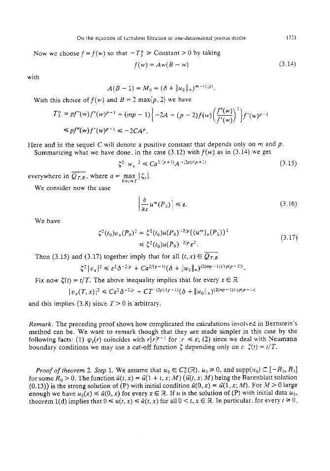
On the equation of turbulent filtration in one-dimensional porous media

Now we choose f = f(w) so that - TT 2 Constant > 0 by taking

f(w) = ‘-tW(B - w)

with

A(B - 1) = M0 = (6 + ~~u&)~+~).

With this choice of f(w) and B = 2 max{p, 2) we have

T; =~f”(w)f’(w)~-’ + (mp - l)[ -2A + (p - 2)~(w)&$j’}~‘(w)p-i

1331

(3.14)

Here and in the sequel C will denote a positive constant that depends only on m and p. Summarizing what we have done, in the case (3.12) with f(w) as in (3.14) we get

?l 1 I.3 12 < CO’ (p+t)A-(2p)/(p+I) 5 I”YrI (3.15)

everywhere in Q T_R, where a = max O<t<T

We consider now the case

&I.

$P(P,) s E.

We have

Then (3.15) and (3.17) together imply that for all (t,~) E QT.R

f21U,12 s $a-?‘P + c,NP+y~ + Ij.,Ilx)(2(mP-l))!(P(P+l)).

Fix now f(r) = r/T. The above inequality implies that for every x E W

/ u,(T, -# < @d-l.P + C‘--(lP)i(P+l)(d + Il~~ll~)(2(mP-l))j(P(P-~J)

and this implies (3.8) since T > 0 is arbitrary.

(3.16)

(3.17)

Remark. The preceding proof shows how complicated the calculations involved in Bernstein’s method can be. We want to remark though that they are made simpler in this case by the following facts: (1) t&,(r) coincides with r/rip-’ for Irj =s E; (2) since we deal with Neumann boundary conditions we may use a cut-off function < depending only on r: c(r) = r/T.

Proof of theorem 2. Step 1. We assume that u. E C;(W), u. 3 0, and supp(uo) C [-Ro, Ro] for some R. > 0. The function ti(t, x) = U(l + t, X; M) (c?(t, x; M) being the Barenblatt solution (0.13)) is the strong solution of (P) with initial condition Li(0, x) = U(1, x; M). For .M > 0 large enough we have uo(x) < a(O, x) for every x E R. If u is the solution of (P) with initial data ~0, theorem l(d) implies that 0 G u(t, x) < G(t, x) for all 0 < t, x E W. In particular. for every t 2 0.

1322 J. R. ESTEBAX and J. L. V.AZQL-EZ

u(f, x) is compactly supported in x. Moreover, given T > 0 we can use the formula for the free boundaries in (0.16) to choose R, > 0 such that supp(rc) is contained in Q = [0, T] x i--R,, R,). In this way K is at the same time the strong (and hence the mild) solution of the Cauchy- Neumann problem

for 0 < t =s T. i.ri < R,

(3.15) Ll(0, x) = Llo(x), for 1x1 < RT

ty iu”(t,?R,) !

=O, forO<t<T

where v(r) = rlriP_‘.

Now for every 0 < 6, E G 1 we consider the solution u,Jt,x) of (3.4) with R = RT. If u~,~ is given by

then lemma 3.3 implies that (3.8) holds for u,,+ Now we set E = a”, u,,~ = u, and (3.8) reads

$ u,(t,x) < c{E’-(“(“P” + t-MP+lyEl!m + IIUoljr)(mP-l):p(p-l)l}, (3.19)

Therefore, rlE(f, x) is x-Holder continuous on [-RT3 RT] with exponent

,=min[l,&]

and coefficient independent on E, 0 < E G 1. Proposition 2.1 and the fact that 14,(0, x) + uo(x) in L’(-RT, R,) as E+ 0 imply that in the

limit u = lim K,, 0 s u(t, x) s jl uOjlr, ~.~(t, x) satisfies the estimate (0.12) and for every- r 2 r > 0 u(t, x) is Holder continuous in x with exponent y and coefficient C,.

Step 2. For general u0 E L’(P?) II L”(!lX), and ug 3 0 we take a sequence u,)., E C;(Z). Us),,, 3 0,

in R ll~~,~L s II4 and ~0.~ - ug in L’([w) as n--f x. For every n the strong solution u,(t, x) of (1.l.a) with initial data Us,,, satisfies 0 < u,(t, x) s 11 urJllx and the estimate of u,,,~ is independent of n.

Since by (0.8) ~4, --, u in C( [0, T]; L’(R))-the solution of (P) with initial data rt,,--the same results hold for 14. In particular u is Holder continuous in x with exponent y.

Step 3. We know that for fixed r > 0 and for every t 2 t; x, y E 2

Iu(t,x) - u(t,y)I 6 Clx -yI?

holds for some C = C(t, mp - 1, IIu,/[~) > 0. We use this fact and the estimate for zli (1.21) to obtain Holder continuity in t. Let (t,,, x0), (tl, x0) be fixed, x0 E R t, > to 2 r > 0. b’e set 6 = ju(t,, x0) - u(to,xo)I, for every x E R we have

6 G 2CIx -xoIy + /14(to,x) - u(t,,x)I


therefore 6

holds for every x E I = {y E W : ly - x01 s (6/2C)“‘}. Then we have

= u,(t, x) dt du

and this means

6 = ]u(t,,xO) - u(to,xO)] S Clt, - roI”(‘+*)

for some C = C(t, m, p, uO) > 0. Then theorem 2(b) holds for u.

Remark. If the initial data has bounded velocity i.e. if

mP oo= ~ i 1 m-Cl/p) mp- 1

UO

satisfies I u; / s K then we can apply the maximum principle instead of Bernstein’s technique in the equation satisfied by u, in the approximate problems (3.4) (this equation can be obtained by differentiating (3.9) with respect to x). In that way the following result is obtained:

THEOREM 3. Under the above conditions we have

/U,(r,X)I +&. (3.20)

This result has been proved by Kalashnikov [14] for the class of weak solutions that he constructs.

SECTION 4

In this section we show how the previous results can be applied to estimate the propagation

properties of the solutions. We consider initial data u. E L’(R), u. 2 0 a.e. and such that

a = ess sup{x E iw : 0 < cco(x)} < +=. (4.1)

Without loss of generality we may assume that a = 0. The fact that the velocity V(r, x) is bounded for all t > 0 implies the existence of a finite right-hand interface defined by

c(r) = sup{x E R : 0 < cc(r, x)}, f(0) = 0. (4.3)

Of course, if supp u. is compact, then supp u(t, . ) is compact and a left-hand interface appears. Its properties are entirely analogous.

We prove the following precise result.

1321 J. R. ESTEBAS and J. L. VAZQUEZ

THEOREM 4. Let u&). ~(t, x), j-(r) as above. Then c(r) is finite for every t 2 0 and c(t) is a nondecreasing, Lipschitz-continuous function [0, x) -+ W which satisfies

for every t 2 0 g(t) < COII.(P(m-I)) Ijl(“Ij(Imp-l) Mm+‘)) (4.3)

and

a.e. t > 0 i”‘(t) s C,t-(P( m+ I)- I). (p(m+ I)) 1/110 [l’l” - ‘b(p(m+ ‘1)

where Co, Ci are positive constants depending on m, p.

(4.4)

Remarks. (1) This result is known both in the porous medium case p = 1, [17,23], and in the case m = 1, cf. [13]. Both consider solutions compactly supported in x. We give the full argument for completeness.

(2) C, is the constant of corollary 1.

Proof of fheorem 4. It follows from (1.21) that the function f--, tm*-i~(t, x) is nondecreasing. In particular, if u(to,x) > 0 and r 2 to > 0, then u(r, X) > 0. Therefore c(r) is nondecreasing. This monotonicity implies that the limit A = ,lirn+ c(t) exists.

To prove that i(t) is finite and (4.3), (4.43 we compare u(t,x) with a family of special solutions of (E) having constant velocity. They are given by

mp _ 1 PhP-l)

U,(f,X) = -

i 1 mP c l.‘bP - 1) [ct - #(mp - 1). (4.5)

First we assume that u. satisfies (4.1) and u. E L’(R) fl L”(R), cl0 2 0. Then for every f > 0, .Y E w

0 S u(t, X) S l/U0 /IX. (4.6)

We compare u(t, X) and fi(t,x) = u,(t, x - x0) in (0 < t < =, 0 <x < x}. Fixing c > 0, choosing x0 such that ]Iuo]ll = Li(0, 0) an d using (4.6). it follows by the maximum principle that

0 S u(t, x) S qt, X) for all t > 0, x E R (4.7)

so that

5‘(t) G x0 + ct = mp c 1 - c-‘/p Ilu,Il!yp) + cr. mp - 1

(4.8)

In particular c(r) < + 2 for every t > 0. Now for every r > 0 fixed we minimize (4.8) with respect to c to get

f(t) < K~MP+U ~Iuo~~~~p-l)l(~+l)

with K = K(m,p) > 0. From this and the smoothing effect (0.10) we obtain (4.3) for every u. E L’(R) as above. Then (4.3) and u E C( [0, x); L’(R)) imply A = 0, i.e. c(t) is continuous at t= 0.

Now we fix to > 0 and set x0 = S;(to), and c = 11 V(to, . )~~z. Next we choose a E 2 such that ]]u~]]~ = u,(O, a - x0) and compare u(t,x) and ti(t, x) = u,(t - ro, x -x0) in {LO < t < r,


a < x < 2) as above to obtain that

c(t) S Qfo) + c(t - to), for all t 3 to > 0.

Finally we let f--, t,,+ to get the Lipschitz-continuity and use (0.17) to obtain (4.1).

REFERENCES

1. ARONSON D. G., Regularity properties of Rows through porous media. SIAMI. appi. Marh. 17.461-467 (1969). 2. BARENBLA~~ G. I., On self-similar motions of compressible fluids in porous media, Prikl. .bfar. .bfek. 16, 679-698

(1952). (In Russian.) 3. BENILAN PH., A strong regularity Lp for solution of the porous media equation, Confriburions to Nonlinear PDE

(Edited by C. BARDOS et a[), Pitman Research Notes No. 86 (1983). 4. BENILAN PH, Sur un probleme d’evolution non monotone dans L’(Q). Publ. Math. Fuc. SC. Besan~on. No. 2

(1976). 5. BENILAN PH., BREZIS H. & CRANDALL M. G., A semilinear equation in L’(w”) Annali Scu. norm. sup. Piss 4,

523-555 (1975). 6. BENILAN PH. & CRANDALL M. G., The continuous dependence on @of the solutions of u, = AQ(u), Indiana Uniu.

Math. /. 30, 161-177 (1981). 7. BENILAN PH. & CRANDALL M. G., Regularizing effects of homogeneous evolution equations. Conaibutions fo

Analysis and Geomerry, supplement to Am. J. Math. (Edited by D. S. CLARK, C. PECELLI and R. SACKSTEDER), pp. 23-29, Baltimore (1981).

8. BREZIS H., Operateurs Maximaux Monotones er Semigroupes de Contraction dans les Espaces de Hilbert, North Holland, Amsterdam (1973).

9. BREZIS H. & PAZY A., Accretive sets and differential equations in Banach spaces, Israel /. Marh. 8, 367-383 (1970.

10. CRANDALL M. G. & LIGGET~ T. M., Generation of semi-groups of nonlinear transformations on general Banach spaces, Am. /. Math. 93, 265-293 (1971).

11. EVANS L. C., Application of nonlinear semigroup theory to certain partial differential equations, Nonlinear Euoiurion Equations (Edited by M. G. CRANDALL), Academic Press. New York (1978).

12. FRIEDMANN A. & KAHIN S., The asymptotic behaviour of a gas in an n-dimensional porous medium, Trans. Am. much. Sot. 262, 551-563 (1980).

13. HERRERO M. A. & VAZQUEZ J. L., On the propagation properties of a nonlinear degenerate parabolic equation, Communs P. D. E. 7, 1381-1402 (1982).

14. KALASHNIKOV A. S., On a nonlinear equation appearing in the theory of non-stationary filtration, Trud. Semin. I.G. Petrooski 4, 137-146 (1978). (In Russian.)

15. KALASHNIKOV A. S., On the propagation of perturbations in the first boundary value problem of a doubly- nonlinear degenerate parabolic equation, Trud. Semin. I. G. Perrouski. Vol. 8, pp. 128-131, (1982). (In Russian.)

16. KAMENO,MOSTSKAYA (KAMIN) SH., The asymptotic behaviour of the solution of the filtration equation, Israel 1. Marh. 14, 76-87 (1973).

17. KNERR B. F., The porous medium equation in one dimension, Trans. Am. mnrh. sot. 234. 381-415 (1977). 18. LZ. C. H., Etude de la classe des operateurs m-accrttifs de f,‘(Q) et accretifs dans L=(D). 3rd cycle thesis, Univ.

Paris VI, (1977). 19. LADY~ENSKMA 0. A., SOLONNIKOV V. A. & URAL’CEVA N. N., Linear an quasilinear equations of parabolic

type, Trunsl. Math. Monogr., American Mathematical Society, Providence, RI (1968). 20. LEIBENSON L. S., General problem of the movement of a compressible fluid in a porous medium, Izu. Akad.

Nauk SSSR, Geography and Geophysics. IX, 7-10 (1945). (In Russian.) 21. PELETIER L. A., The porous media equation, Applications of Nonlinear Analysis in the Physical Sciences (Edited

by H. A,MANN er nl.), pp. 229-241, Pitman, London, (1981). 22. VAZQUEZ J. L., Asymptotic behaviour and propagation properties of the one-dimensional fioa of gas in a porous

medium, Trans. Am. marh. Sot. 277, 507-527 (1983). 23. VAZQUEZ J. L., The interface of one-dimensional flows in porous media, Trans. Am. marh. Sot. 285, 717-737

(1984). 24. VAZQUEZ J. L., Symetrisation pour u, = A+(u) et applications, C.R. hebd. seanc. Acad. Sci. Paris 295, 71-71

(1982). 25. VAZQUEZ J. L., Symmetrization in nonlinear parabolic equations, Porruguiiae Math. 41. 339-3-16 (1982). 26. WIDDER D. V., The Hem Equation, Academic Press, New York (1975).

On the equation of turbulent filtration in one- dimensional porous media

Documents

Transcript of On the equation of turbulent filtration in one- dimensional porous media