arX

iv:m

ath/

0105

228v

1 [

mat

h.A

P] 2

8 M

ay 2

001

FILTRATION LAW FOR POLYMER FLOW THROUGH POROUS MEDIA

Alain Bourgeat Olivier GipoulouxFaculte des sciences et techniques, Universite de St-Etienne

23 Rue Dr Paul Michelon, 42 023 St-Etienne Cedex 2, France

Eduard Marusic-PalokaDepartment of Mathematics, University of Zagreb,

Bijenicka 30, 10000 Zagreb, Croatia

1

Abstract. In this paper we study the filtration laws for the polymeric flow in a porous medium. We use

the quasi-Newtonian models with share dependent viscosity obeying the power-law and the Carreau’s law. Using

the method of homogenization in [5] the coupled micro-macro homogenized law, governing the quasi-newtonian

flow in a periodic model of a porous medium, was found. We decouple that law separating the micro from the

macro scale. We write the macroscopic filtration law in the form of non-linear Darcy’s law and we prove that the

obtained law is well posed. We give the analytical as well as the numerical study of our model.

1 Introduction

It is well-known that the viscosity of a polymer melt or a polymer solution significantly changes with theshare rate (see e.g. [1]). Therefore the Newtonian model, characterized by a constant viscosity, is not areasonable choice for modelling the polymeric flow. The simplest way to overcome that difficulty is touse the notion of quasi-Newtonian flow, i.e. to modify the Newton’s model by using the variable viscositythat depends on the share-rate according to some empirical law. In this paper, in order to describe thepolymer flow, we use the share dependent viscosities obeying the power-law

η(e(u)) = µ|e(u)|r−2e(u) , 1 < r < 2 , µ > 0 (1)

or the Carreau’s law

η(e(u)) = (η0 − η∞)(1 + λ|e(u)|2)r/2−1 + η∞ , 1 < r < 2 , η0 > η∞ ≥ 0 , λ > 0 , (2)

where

e(u) =1

2(∇u + ∇ut) the rate-of-strain tensor ,

|e(u)| = (

n∑

i,j=1

|e(u)ij |2)1/2 − the share rate ,

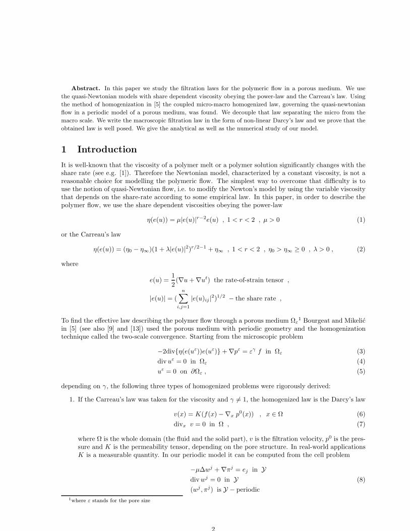
To find the effective law describing the polymer flow through a porous medium Ωε1 Bourgeat and Mikelic

in [5] (see also [9] and [13]) used the porous medium with periodic geometry and the homogenizationtechnique called the two-scale convergence. Starting from the microscopic problem

−2divη(e(uε))e(uε) + ∇pε = εγ f in Ωε (3)

div uε = 0 in Ωε (4)

uε = 0 on ∂Ωε , (5)

depending on γ, the following three types of homogenized problems were rigorously derived:

1. If the Carreau’s law was taken for the viscosity and γ 6= 1, the homogenized law is the Darcy’s law

v(x) = K(f(x) −∇x p0(x)) , x ∈ Ω (6)

divx v = 0 in Ω , (7)

where Ω is the whole domain (the fluid and the solid part), v is the filtration velocity, p0 is the pres-sure and K is the permeability tensor, depending on the pore structure. In real-world applicationsK is a measurable quantity. In our periodic model it can be computed from the cell problem

−µ∆wj + ∇πj = ej in Ydiv wj = 0 in Y (8)

(wj , πj) is Y − periodic

1where ε stands for the pore size

2

by

Kij =

∫

Y

wij = µ

∫

Y

∇wi∇wj , (9)

where Y ⊂]0, 1[n is the fluid part of the unit cell (the period) Y =]0, 1[n and S is the boundary ofits solid part A = Y \Y of Y . The viscosity µ is equal to η0, in case γ < 1 and to η∞ if γ > 1 andη∞ > 0. Defining

u0(x, y) =

n∑

i=1

wi(y)∂p0

∂xi(x) , p1(x, y) =

n∑

i=1

πi(y)∂p0

∂xi(x) ,

the above filtration law (6) and the cell problem (8) can be written in the coupled form

−µ ∆y u0 + ∇yp1 = f(x) −∇xp0(x) in Ω × Y (10)

divyu0 = 0 in Ω × Y (11)

(u0, p1) is Y − periodic in y (12)

divx

(∫

Y

u0 dy

)

= 0 in Ω (13)

u0 = 0 on Ω × S (14)

n ·(∫

Y

u0 dy

)

= 0 on ∂Ω . (15)

Two functions u0 and p1 are, in fact, first oscillating terms in the asymptotic expansion for thevelocity and for the pressure, respectively.

2. If the viscosity obeys the Carreau’s law with γ = 1, the homogenized law is the coupled Carreau’slaw

−divyηc(ey(u0))ey(u0) + ∇yp1 = f(x) −∇xp0(x) in Ω × Ydivyu0 = 0 in Ω × Y (16)

(u0, p1) is Y − periodic in y

divx

(∫

Y

u0 dy

)

= 0 in Ω

u0 = 0 on Ω × S

n ·(∫

Y

u0 dy

)

= 0 on ∂Ω ,

ηc(ξ) = (η0 − η∞)(1 + λ|ξ|2)r/2−1 + η∞ . (17)

Here p0 is the pressure and

v =

∫

Y

u0(x, y) dy

is the filtration velocity. Functions u0(x, y) and p1(x, y) are oscillating in y and, in analogy withthe linear case, can be seen as the first oscillating terms in the asymptotic expansion of the flow.

3. In case of power-law, the homogenized law is the coupled power-law

−divyηp(ey(u0))ey(u0) + ∇yp1 = f(x) −∇xp0(x) in Ω × Ydivyu0 = 0 in Ω × Y(u0, p1) is Y − periodic in y (18)

divx

(∫

Y

u0 dy

)

= 0 in Ω

3

u0 = 0 on Ω × S

n ·(∫

Y

u0 dy

)

= 0 on ∂Ω ,

ηp(ξ) = µ|ξ|r−2ξ . (19)

In case 1 two scales are separated and the filtration law is completely macroscopic. All the microscopicinformation are contained in the permeability tensor K, which can be measured in applications. In cases2 and 3 the situation is different and two scales are still coupled. Even if, mathematically speaking, thoseresults solve the homogenization problem for such fluids, to get a physically relevant result one needs todecouple the problems and to find the filtration laws in the usual macroscopic form

v = U(f −∇xp0) (20)

where

v(x) =

∫

Y

u0(x, y) dy .

Using the idea from [3], [4] and [12] to decouple the homogenized problems we define the auxiliary problem

−divyηα(ey(wξ))ey(wξ) + ∇yπξ = ξ in Y (21)

divywξ = 0 in Y (22)

(wξ, πξ) is Y − periodic (23)

wξ = 0 on S , α = c, p . (24)

With (wξ, πξ) we define the permeability function U : Rn → Rn by

U(ξ) =

∫

Y

wξ(y) dy , (25)

and we obtain formally the filtration law (20). From the definition we can obviously conclude that thefunction U is odd, i.e. that

U(−ξ) = −U(ξ) .

From (18) we also getdiv v = 0 in Ω , v · n = 0 on ∂Ω . (26)

To show that (18) and (20)-(26) are equivalent, we prove in sections 2 and 4 that U is monotone andcoercive, consequently, that (20)-(26) is well posed.We also perform the qualitative analysis of the permeability function U . In case of coupled Carreau’slaw, we find its Taylor’s expansion.

2 The Carreau’s coupled homogenized problem

In this section we use the notation η for the Carreau’s viscosity ηc, i.e. we omit the index c. We beginthis section with statement of the main results

3 Statement of the main result

To prove that our formal separation of the coupled problem is meaningful we have to prove that ourmacroscopic problem has a unique solution.

4

Theorem 1 Let U : Rn → Rn be defined by (25). Then the macroscopic problem

div U(f −∇p0) = 0 in Ω (27)

n · U(f −∇p0) = 0 on ∂Ω (28)

has a unique (up to a constant) solution p0 ∈ W 1,r′

(Ω), for any f ∈ Lr′

(Ω)n.

In order to approximate the permeability function U in vicinity of 0 we compute its Taylor’s expansion.First two terms can be written in the form

U(ξ) = Kξ +1

2(η0 − η∞)λ(2 − r)

n∑

m,j,k,ℓ=1

Hℓmjk ξjξkξℓ em + O(|ξ|5) , (29)

where K is the classical Darcy’s permeability and the coefficients Hℓmjk are defined by (55). S uch

approximate filtration law, given by the polynomial permeability

V(ξ) = Kξ +1

2(η0 − η∞)λ(2 − r)

n∑

m,j,k,ℓ=1

Hℓmjk ξjξkξℓ em

is still well posed:

Theorem 2 Let f ∈ L4(Ω)n . The problem

div V(f −∇q0) = 0 in Ω (30)

n · V(f −∇q0) = 0 on ∂Ω (31)

has a unique (up to a constant) solution q0 ∈ W 1,4(Ω).

3.1 Taylor’s expansion of the permeability function

We want to find the Taylor’s expansion for U in vicinity of 0. Since the function is odd all the derivativesof a pair order DαU(0) , |α| = 2m , m ∈ N are equal to 0. Deriving (21) with respect to ξj we find

Theorem 3 Let K be the Darcy’s permeability tensor computed from the local problem

−η0∆wj + ∇πj = ej in Ydiv wj = 0 in Y (32)

(wj , πj) is Y − periodic

by

Kij =

∫

Y

wij = η0

∫

Y

∇wi∇wj . (33)

Then∇ξU(0) = K (34)

To prove that we proceed as in [3], [4] or [12]. We begin by recalling the result from [14]:

Lemma 1 There exist a constant cr1 > 0 such that :

cr1

|e(v − u)|2Lr(Y)

1 + |e(u)|2−rLr(Y) + |e(v)|2−r

Lr(Y)

≤∫

Y

[η(e(u))e(u) − η(e(v))e(v)] e(u − v) (35)

for anyu, v ∈ W = φ ∈ W 1,r(Y)n ; div φ = 0 , φ is Y − periodic , φ = 0 on S .

5

Lemma 2 Let (wξ, πξ) ∈ W × L2(Y) be defined by (21)-(24). Then

|e(wξ)|Lr(Y) ≤ 2Cr

cr1

|Y|1− 1

r |ξ| , (36)

for any ξ such that

|ξ| <cr1

2Cr|Y|1− 1

r

,

where Cr is the Poincare-Korn’s constant in W (i.e. such that |φ|Lr(Y) ≤ Cr|e(φ)|Lr(Y) ∀ φ ∈ W ).

Proof. Multiplying (21) by wξ and integrating over Y we obtain

ξ ·∫

Y

wξ =

∫

Y

η(e(wξ))e(wξ) ≥ cr1

|e(wξ)|2Lr(Y)

1 + |e(wξ)|2−rLr(Y)

.

Now (35) gives

cr1|e(wξ)|Lr(Y) ≤ Cr|Y|1− 1

r (1 + |e(wξ)|2−rLr(Y)) |ξ| .

If |e(wξ)|Lr(Y) < 1 then (36) obviously holds. On the other hand, supposing that |e(wξ)|Lr(Y) > 1, implies

cr1|e(wξ)|Lr(Y) ≤ 2Cr|Y|1− 1

r |e(wξ)|2−rLr(Y) |ξ|

and

|e(wξ)|r−1Lr(Y) ≤ 2

Cr

cr1

|Y|1− 1

r |ξ|

which contradicts the assumption that

|ξ| <cr1

2Cr|Y|1− 1

r

. ♣

Proof of theorem 3. To prove the claim we only need to show that, as |h| → 0

|wh − W (h)|W = o(|h|) , W (h) =

n∑

i=1

hi wi (37)

because

|U(h) − K h| = |∫

Y

[wh − W (h)]| ≤ C|wh − W (h)|W . (38)

In fact we shall prove that|U(h) − K h| = O(|h|3) (39)

which implies, not only that ∇U(0) = K, but also that ∇2U(0) = 0 (which we knew before because U isan odd function). Using the standard regularity result (see e.g. [6]) for the problem (32) we see that

|W (h)|H3(Y) ≤n∑

i=1

|h| |wi|H3(Y) ≤ C |h| . (40)

and therefore|W (h)|C1(Y) ≤ C |h| . (41)

Functions W (h) and Π(h) =∑n

i=1 hi πi satisfy the system

−divηe[W (h)]e[W (h)] + ∇Π(h) = h + Rh (42)

div W (h) = 0 (43)

(W (h), Π(h)) is Y − periodic , W (h) = 0 on S , (44)

6

whereRh = div(η0 − η∞)[(1 + λ|e[W (h)]|2)r/2 −1 − 1]e[W (h)] .

An easy computation leads to

(1 + λt2)r/2−1 − 1 = (r/2 − 1)t2∫ λ

0

(1 + τt2)r/2−2dτ ≤ Ct2 .

For 1 < r < 2 we get using (41)

∫

Y

Rh φ ≤ C|φ|W 1,r(Y)| |e[W (h)]|3L3r′ (Y)

≤ C|h|3|φ|W 1,r(Y) . (45)

Subtracting (21) from (42), multiplying by W (h) − wh and integrating over Y we obtain

J =

∫

Y

ηe[W (h)]e[W (h)] − ηe(wh)e(wh) e(W (h) − wh) =

=

∫

Y

Rh(W (h) − wh) ≤ C|h|3|W (h) − wh|W .

An application of lemma 1 gives

J ≥ cr1

|W (h) − wh|2W1 + C|h| . ♣

As we have seen the second derivative in ξ = 0 is 0. Third can be computed from the auxiliary problem

−η0∆wℓjk + ∇πℓjk = (46)

= (η0 − η∞)(r − 2)λdive(wk) · e(wj) e(wℓ) + (47)

+e(wk) · e(wℓ) e(wj) + e(wℓ) · e(wj) e(wk) in Y (48)

div wijk = 0 in Y (49)

(wijk , πijk) is Y − periodic (50)

by∂3U(0)

∂ξℓ∂ξj∂ξk=

∫

Y

wℓjk .

Since

∂3U(0)m

∂ξℓ∂ξj∂ξk= η0

∫

Y

∇wℓjk∇wm = (51)

= (η0 − η∞)(2 − r)λ

∫

Y

e(wk) · e(wj) e(wℓ) · e(wm) + (52)

+e(wk) · e(wℓ) e(wj) · e(wm) + e(wℓ) · e(wj) e(wk) · e(wm) = (53)

= (η0 − η∞)(2 − r)λ(Hℓmjk + Hjm

ℓk + Hkmℓj ) , (54)

where

Hℓmjk = Hmℓ

jk = Hℓmkj = Hjk

ℓm =

∫

Y

e(wk) · e(wj) e(wℓ) · e(wm) . (55)

This gives the expansion for U in the form

U(ξ) = Kξ +1

2(η0 − η∞)λ(2 − r)

n∑

m,j,k,ℓ=1

Hℓmjk ξjξkξℓ em + O(|ξ|5) . (56)

7

Proposition 1 Let Hℓmjk be defined by (55). Then (56) holds.

Proof. We use the same idea as in the proof of theorem 3. We define

V (h) =

n∑

i+1

wihi +1

2

n∑

i,j,k=1

wijkhihjhk

Q(h) =

n∑

i+1

πihi +1

2

n∑

i,j,k=1

πijkhihjhk .

Now

−divηr(e[V (h))]e(V (h)) + ∇Q(h) =

= h − (η0 − η∞)div[1 + λ|e(V (h))|2)r/2−1 − 1]e[V (h)] +

+λ

2(r − 2)(η0 − η∞)div

n∑

i,j,m=1

e(wi) · e(wj) e(wm) hihjhm .

It only remains to estimate

J = (η0 − η∞)div[1 + λ|e(V (h))|2)r/2−1 − 1]e[V (h)] +

+λ

2(r − 2)(η0 − η∞)div

n∑

i,j,m=1

e(wi) · e(wj) e(wm) hihjhm .

A simple Taylor’s formula gives

(1 + λ|ξ|2)r/2−1 − 1 =1

2λ|ξ|2 + O(λ2|ξ|4) .

After recalling that e(wi) ∈ C(Y)n×n , e(wijk) ∈ C(Y)n×n, we get for any y ∈ Y

(η0 − η∞)div[1 + λ|e(V (h))|2)r/2−1 − 1]e[V (h)] =

=λ

2(r − 2)(η0 − η∞)div

n∑

i,j,m=1

e(wi) · e(wj) e(wm) hihjhm + O(|h|4) .

Arguing as in the proof of theorem 3, we get the claim. ♣

Remark 1 It can be seen from the definition that Hiijj > 0 , Hℓk

ℓk > 0. Furthermore, for

Z(h) =

n∑

i,j,k,ℓ=1

Hiℓjkhjhkhi eℓ =

∫

Y

|n∑

k=1

e(wk)hk|2n∑

i=1

e(wi)hi

n∑

ℓ=1

e(wℓ) eℓ

we have

Z(h) · h =

∫

Y

|n∑

k=1

e(wk)hk|2 > 0 .

To compute further order terms we proceed in the same way and we get another auxiliary problem

−η0∆wijkℓp + ∇πijkℓp = (57)

= (η0 − η∞)λ(r − 2)div (58)

e(wi) · e(wj)e(wkℓm) + e(wk) · e(wi)e(wjℓm) + e(wi) · e(wℓ)e(wjkm) + (59)

e(wi) · e(wp)e(wjkℓ) + e(wj) · e(wk)e(wiℓm) + e(wj) · e(wℓ)e(wikm) + (60)

e(wj) · e(wp)e(wikℓ) + e(wk) · e(wℓ)e(wijm) + e(wk) · e(wp)e(wijℓ) + (61)

8

e(wℓ) · e(wp)e(wijk) + (62)

(e(wjkℓ) · e(wi) + e(wikℓ) · e(wj) + e(wijℓ) · e(wk) + e(wijk) · e(wℓ))e(wp) + (63)

(e(wjkm) · e(wi) + e(wikm) · e(wj) + e(wijm) · e(wk) + e(wijk) · e(wp))e(wℓ) + (64)

(e(wjℓm) · e(wi) + e(wiℓm) · e(wj) + e(wijm) · e(wℓ) + e(wijℓ) · e(wp))e(wk) + (65)

(e(wkℓm) · e(wi) + e(wiℓm) · e(wk) + e(wikm) · e(wℓ) + e(wikℓ) · e(wp))e(wj) + (66)

(e(wkℓm) · e(wj) + e(wjℓm) · e(wk) + e(wjkm) · e(wℓ) + e(wjkℓ) · e(wp))e(wi) + (67)

λ(r − 4) (68)

e(wℓ) · e(wk)e(wj) · e(wi) + e(wℓ) · e(wj)e(wk) · e(wi) + e(wℓ) · e(wi)e(wk) · e(wj)e(wp) + (69)

e(wp) · e(wk)e(wj) · e(wi) + e(wp) · e(wj)e(wk) · e(wi) + e(wp) · e(wi)e(wk) · e(wj)e(wℓ) +(70)

e(wp) · e(wℓ)e(wj) · e(wi) + e(wp) · e(wj)e(wℓ) · e(wi) + e(wp) · e(wi)e(wℓ) · e(wj)e(wk) + (71)

e(wp) · e(wℓ)e(wk) · e(wi) + e(wp) · e(wk)e(wℓ) · e(wi) + e(wp) · e(wi)e(wℓ) · e(wk)e(wj) +(72)

e(wp) · e(wℓ)e(wk) · e(wj) + e(wp) · e(wk)e(wℓ) · e(wj) + e(wp) · e(wj)e(wℓ) · e(wk)e(wi)(73)

div wijkℓp = 0 in Y (74)

(wijkℓp, πijkℓp) is Y − periodic . (75)

Now∂5U(0)

∂ξi∂ξj∂ξk∂ξℓ∂ξp=

∫

Y

wijkℓp

and we get an expansion in the form

U(ξ) = Kξ +1

2(η0 − η∞)λ(2 − r)

n∑

i,j,k,ℓ,m=1

Hℓmjk ξjξkξℓ em +

+1

2(η0 − η∞)λ(2 − r)

n∑

j,k,ℓ,m,p,q=1

Hmpqjkℓ ξjξkξℓξmξp eq + O(|ξ|7)

where

Hmpqjkℓ =

∫

Y

e(wj) · e(wk) e(wℓmp) · e(wq) + λ(r − 4)

2e(wj) · e(wk) e(wℓ) · e(wm) e(wp) · e(wq) .

This computation can be proceeded.

9

3.2 Proofs of existence theorems

To prove the theorem 3 we first prove the following lemma that gives coercivity and boundness of thedifferential operator

A(φ) = −divU(f −∇φ) .

Lemma 3 There exist constants M, C, c > 0 such that

U(ξ) · ξ ≥ c|ξ|r′

for any |ξ| > M (76)

|U(ξ)| ≤ C|ξ|r′−1 for any ξ ∈ Rn . (77)

Proof. The upper bound is easy to prove, since we have, due to (35)

cr1

|e(wξ)|Lr(Y)

|e(wξ)|2−rLr(Y) + 1

≤ C|ξ| .

To prove the lower bound (76) we define vξ = |ξ|1−r′

wξ and qξ = |ξ|−1 ξ. Those functions satisfy thesystem

−divyηξ(ey(vξ))ey(vξ) + ∇yqξ =ξ

|ξ| in Y (78)

divyvξ = 0 in Y (79)

(vξ, qξ) is Y − periodic (80)

vξ = 0 on S , (81)

whereηξ(τ) = (η0 − η∞)(|ξ|2(1−r′) + λ|τ |2)r/2 −1 + η∞|ξ|−r′

.

Applying again (35) we obtain|e(vξ)|Lr(Y)

|ξ|2(1−r′)(2−r) + |e(vξ)|Lr(Y)

≤ C

so that we can extract a subsequence ξn such that |ξn| → ∞ , |ξn|−1 ξn → ξ∞ , |ξ∞| = 1 and

vξn v∞ weakly in W as n → ∞ .

Using the Minty’s lemma we get that v∞ satisfies the system

−(η0 − η∞)λr/2 −1 divy|ey(v∞))|r−2ey(v∞) + ∇yq∞ = ξ∞ in Ydivyv∞ = 0 in Y(v∞, q∞) is Y − periodic

v∞ = 0 on S ,

For any ξ∞, such that |ξ∞| = 1, we can define a continuous function

I(ξ∞) =

∫

Y

v∞ 6= 0 .

Furthermore

I(ξ∞) · ξ∞ =

∫

Y

(η0 − η∞) λr/2 −1 |e(v∞)|r .

and there existsc∞ = inf

|τ |=1I(τ) · τ > 0 .

10

Two functionals

Φξ(v) =

∫

Y

ηξ(e(v)) |e(v)|2

Φ∞(v) =

∫

Y

(η0 − η∞) λr/2 −1 |e(v)|r

are obviously convex and, due to the Lebesgues dominated convergence theorem,

Φξ(vξ) − Φ∞(vξ) → 0 as |ξ| → ∞ .

Since Φ∞ is weak lower semicontinuous in W , we obtain

lim|ξ|→∞

inf Φξ(vξ) = lim|ξ|→∞

infΦ∞(vξ) + [Φξ(vξ) − Φ∞(vξ)] ≥ Φ∞(v∞) ≥ c∞ > 0 .

ButΦξ(vξ) = |ξ|−r′ U(ξ) · ξ

which proves the claim. ♣Proof of theorem 3. Lemma 3.2 implies coercivity and boundness of the operator A : W 1,r′

(Ω)/R →(W 1,r′

(Ω))′ . Its strict monotonicity follows from inequality

[U(ξ) − U(τ)] · (ξ − τ) =

∫

Y

ηc(e(wξ))e(wξ) − ηc(wτ ))] · (wξ − wτ )

≥ cr1

|e(wξ − wτ )|2Lr(Y)

|e(wξ)|2−rLr(Y) + |e(wτ )|2−r

Lr(Y) + 1.

Now the classical Browder-Minty’s theorem proves the existence of the solution, i.e. the surjecivity ofour operator. As it is strictly monotone, it is also injective, i.e. the solution is unique. ♣

If we approximate U by taking only first two terms in its Taylor’s series, i.e., if we consider

V(ξ) = Kξ +1

2(η0 − η∞)λ(2 − r)

n∑

m,j,k,ℓ=1

Hℓmjk ξjξkξℓ em

instead of U , we get the problem (30)-(31).For such approximation of the filtration law we have theorem 2, from the beginning of this section. Weare now able to prove it.Proof of theorem 2. We define the formal differential operator

B(ϕ) = divV(f −∇ϕ) .

Since V is a polynomial of order 3, it satisfies the estimate

|V(ξ)| ≤ C (|ξ| + |ξ|3) .

Consequently B : W 1,4(Ω)/R → (W 1,4(Ω)/R)′ is a bounded operator. Moreover

|B(ϕ)|(W 1,4(Ω)/R)′ ≤ C |f −∇ϕ|3L4(Ω) .

Next we prove the coercivity. Let

E(ξ) =n∑

i=1

e(wi) ξi .

Then, for any ξ ∈ Rn,

V(ξ) · ξ =

∫

Y

( η0 |E(ξ)|2 + (η0 − η∞) λ(1 − r/2)|E(ξ)|4 ) .

11

The functions

G(ξ) =

∫

Y

|E(ξ)|2 , H(ξ) =

∫

Y

|E(ξ)|4

are continuous and strictly positive for ξ 6= 0. Therefore there exist

κ1 = inf|ξ|=1

G(ξ) , κ2 = inf|ξ|=1

H(ξ) .

But thanV(ξ) · ξ ≥ κ1 |ξ|2 + (η0 − η∞) λ (1 − r/2) κ |ξ|4 ,

implying the coercivity of B on W 1,4(Ω)/R. It remains to prove the monotonicity of B. Then the resultwill follow from the classical Browder-Minty’s theorem.For any ξ, τ ∈ Rn the derivative DV(ξ) satisfies

DV(ξ) τ · τ = Kτ · τ +1

2λ(2 − r)(η0 − η∞)

∫

Y

[(E(ξ) · E(τ))2 +

+E(ξ)2 E(τ)2] > Kτ · τ ≥ k0|τ |2 .

The above inequality proves that the equation (30) is uniformly elliptic , i.e. that the operator B ismonotone. ♣

The approximation V of the permeability function is valid either for small |ξ| or for small λ. For large λand |ξ|, the Carreau’s auxiliary problem (21)-(24), with ηc, is close to the power-law auxiliary problem(21)-(24), with ηp and µ = (η0 − η∞)λr/2−1. We study the power-law auxiliary problem in the nextsection.We refer to section 6.3 for numerical computation of the permeability function U and its approximationV and their comparison for sufficiently small |ξ|.

4 The power-law coupled homogenized problem

In this section we also start with statement of its main results and we adopt the notation η for thepower-law viscosity ηp.

5 Statement of the main result

From (21)-(25) we get by substitution that the permeability function is homogeneous in the sense that

U(λ ξ) = |λ|r′−2 λU(ξ) , λ ∈ R . (82)

implyingm|ξ|r′−1 ≤ |U(ξ)| ≤ M |ξ|r′−1 (83)

withm = inf

|ξ|=1|U(ξ)| , M = sup

|ξ|=1

|U(ξ)| .

Now, as in the previous chapter, (83) and (88) imply that:

Theorem 4 For any f ∈ Lr′

(Ω)n the macroscopic problem

divU(f −∇p0) = 0 in Ω (84)

n · U(f −∇p0) = 0 on ∂Ω (85)

has a unique (up to a constant) solution p0 ∈ W 1,r′

(Ω).

12

The standard engineering model (see e.g. [2], [15]) suggests that the permeability function U can bewritten in the form

U(ξ)i = |(K ξ)i|r′−2 (K ξ)i , i = 1, . . . , n , (86)

where K is a permeability tensor.To check that conjecture we define the conjugated function G by

G(ξ)i = |U(ξ)i|r−2 U(ξ)i ,

such thatU(ξ)i = |G(ξ)i|r

′−2 G(ξ)i .

Now, if the conjecture (86) is true, the function G is linear. Homogeneity (82) of U implies that G ishomogeneous with order 1, i.e. that

G(λ ξ) = λG(ξ) , λ ∈ R .

Function homogeneous with order 1 is linear if and only if it is differentiable for ξ = 0.Function G is differentiable for any ξ 6= 0, but, in general, not for ξ = 0. That means that the conjecture(86) is, in general, false. In case of unidirectional flow it is differentiable and, therefore, linear. Incase of a porous medium consisting of a net of narrow channels, G allows an asymptotic expansion inpowers of the thickness of the channels, with the first term being a linear function. Numerical examplesshow that G is linear (or differentiable for ξ = 0) in case of periodic porous medium with the solid partbeing an array of rectangular obstacles (i.e. with the fluid part being a net of perpendicular channels).On the other hand, in case of spherical or elliptical obstacle, the function G is not linear and conjecture(86) does not hold.

5.1 Study of the permeability function

We next recall the result from [14], that will be used in the sequel:

Lemma 4 There exist a constant cr1 > 0 such that :

cr1

|e(v − u)|2Lr(Y)

|e(u)|2−rLr(Y) + |e(v)|2−r

Lr(Y)

≤∫

Y

[η(e(u))e(u) − η(e(v))e(v)] e(u − v) (87)

for anyu, v ∈ W = φ ∈ W 1,r(Y)n ; div φ = 0 , φ is Y − periodic , φ = 0 on S .

It implies that, for ξ, τ ∈ Rn, ξ 6= τ ,

[U(ξ) − U(τ)] · (ξ − τ) ≥ cr1

|e(wξ − wτ )|2Lr(Y)

|e(wξ)|2−rLr(Y) + |e(wτ )|2−r

Lr(Y)

> 0 . (88)

Before we continue we give two simple examples mentioned in the introduction of this section.

Example 1 As it was noticed in [5], [13], [9], if the flow is unidirectional, e.g. in the direction e1, thenU(ξ) = J (ξ1) e1, with

J (ξ1) = |ξ1|r′−2 ξ1 .

This result corresponds to the usual models that can be found in the engineering literature (see e.g. [15],[7]).

13

Example 2 In case of a porous medium consisting of a network of thin pipes we can find the asymptoticform of our function U and, again, it corresponds to the usual engineering model from [7] and [15].Suppose that n = 2 and that Y = Yδ consists of two narrow perpendicular channels

P 1δ =]0, 1[ × ] − δ/2, δ/2 [ , P 2

δ = ] − δ/2, δ/2 [ × ]0, 1[ ,

with thickness δ. We consider our auxiliary problem in such unit cell Yδ = P 1δ ∪ P 2

δ

−divyηp(ey(wδξ ))ey(wδ

ξ) + ∇yπδξ = ξ in Yδ (89)

divywδξ = 0 in Yδ (90)

(wξ, πξ) is Yδ − periodic (91)

wξ = 0 on Sδ , (92)

where Sδ = ∂(P 1δ ∪ P 2

δ ). We study the limit as δ → 0. The similar problem was considered in [11] forthe Newtonian fluid and an explicit formula for the permeability was found. We are going to do the samething with our nonlinear permeability function Uδ(ξ) =

∫

Y wδξ . As in [11], we seek an approximation of

(wδξ , πδ

ξ) in the form

w(δ) = δr′

θ(y2/δ) |ξ1|r′−2ξ1 e1 in P δ

1

θ(y1/δ) |ξ2|r′−2ξ2 e2 in P δ

2

, π(δ) =

y2 ξ2 in P δ1

y1 ξ1 in P δ2

where

θ(z) =2

r′ µ

(√2

µ

)r′−2

[ (1/2)r′ − |z|r′

] .

In each P iδ we have the Poincare-Korn’s inequality

|wδξ − w(δ)|Lr(P i

δ) ≤ Cδ|e(wδ

ξ − w(δ))|Lr(P iδ)

and the trace inequality

|wδξ − w(δ)|Lr(Σi

δ) ≤ C δ1/r′ |e(wδ

ξ − w(δ))|Lr(P iδ) ,

whereΣ1

δ = ∂P 1δ ∩ P 2

δ , Σ2δ = ∂P 2

δ ∩ P 1δ .

By a direct computation we obtain

µ

∫

P iδ

|e(wδξ)|r−2e(wδ

ξ) − |e(w(δ))|r−2e(w(δ))e(wδξ − w(δ)) =

=

∫

Σiδ

π(δ)n − µ|e(w(δ))|r−2e(w(δ))n (wδξ − w(δ)) .

We use (87) to estimate from below the left-hand side and the above inequalities to estimate from abovethe right-hand side. It leads to the estimate

|δ−(1+r′) Uδ(ξ) − 〈θ〉 J (ξ) | ≤ C δ1/r ,

where

〈θ〉 =

∫ 1/2

−1/2

θ(s)ds =2

(r′ + 1)µ(√

2/µ)r′−2 ,

andJ (ξ) = (|ξ1|r

′−2ξ1, |ξ2|r′−2ξ2) .

14

Therefore

Uδ(ξ)i = δr′+1 2

(r′ + 1)µ(√

2/µ)r′−2 |ξi|r′−2 ξi + O(δr′+1+1/r) , i = 1, 2

i.e.Uδ(ξ) ≈ CδJ(ξ) .

We are now tempted to believe that the permeability function can be written in the form (86).First of all, we can not hope to have K that depends only on the geometry of the porous medium, as inthe linear case, because in two above examples it depends on the flow index r.We know that this conjecture is true in case of unidirectional flow and, up to some order of approximation,for a network of narrow channels.

To verify whether (86) is true or not, we define the conjugated permeability function

G(ξ)i = |U(ξ)i|r−2U(ξ)i , i = 1, . . . , n .

As r−2 < 0 and U(0) = 0 , G(0) is not correctly defined by the above formula. However, since U satisfies(82), and (83)we have

m|ξ| ≤ |G(ξ)| ≤ M |ξ| .

Therefore we define G in ξ = 0 by G(0) = 0 and we get the function G ∈ C(R)n . Function G is obviouslyhomogeneous

G(λ ξ) = λG(ξ) .

we refer to the section 6.4 where a numerical example shows that in case of bundle of perpendicular,not necessarily narrow, channels G is differentiable and linear, i.e. that (86) can be expected to holdin rectangular geometry. That can be explained by the fact that we have n unidirectional flows with,almost, no interaction between them. In fact, example 2 proves that the interaction between two flowsexists, but it has some lower order.As it was noticed in [13] the function U is differentiable for any ξ 6= 0. We are, therefore, in situationvery close to (86). Moreover

∂U(ξ)i

∂ξj=

∫

Y

[wjξ(y)]i dy , (93)

where

−µ divy(r − 2)|ey(wξ)|r−4 [e(wξ) · e(wjξ)] ey(wξ) + (94)

+|ey(wξ)|r−2ey(wjξ) + ∇yπj

ξ = ej in Y (95)

divywjξ = 0 in Y

(wjξ , π

jξ) is Y − periodic

wjξ = 0 on S . (96)

Since this problem is linear it is easy to prove the following result:

Proposition 2 For ξ 6= 0 the problem (95)-(96) has a unique solution wiξ ∈ Vξ, where

Vξ = φ ∈ W 1,r# (Y)n ; |e(wξ)|

r2−1e(φ) ∈ L2(Ω) , div φ = 0

andW 1,r

# (Ω) = φ ∈ W 1,r(Y) ; wjξ is Y − periodic , wj

ξ = 0 on S .

Furthermore wjξ satisfies the a priori estimate

|e(wjξ)|Lr(Y) ≤ C |e(wξ)|2−r

Lr(Y) . (97)

15

Proof. We first notice that the definition of Vξ has a sense since, due to the (21), e(wξ) 6= 0 (a.e) in Y.Now Vξ is the Banach space equipped by the norm

|φ|Vξ= |e(φ)|Lr(Y) + | |e(wξ)|

r2−1e(φ)|L2(Y) .

The operator T : Vξ → V ′ξ , defined by

T φ = −µ divy(r − 2)|ey(wξ)|r−4 [e(wξ) · e(φ)] ey(wξ) + |ey(wξ)|r−2ey(φ)

is coercive since, using the Holder’s inequality, we get

〈Tφ|φ〉 ≥ (r − 1)

∫

Y

|e(wξ)|r−2 |e(φ)|2

≥ r − 1

2| |e(wξ)|

r2−1e(φ)|2L2(Ω) + (|e(wξ)|Lr(Y))

(r−2)|e(φ)|2Lr(Y) .

Now T ∈ L(Vξ, V′ξ ) is linear and coercive. Therefore it is bijective. The estimate (97) follows from

〈T wjξ |w

jξ〉 ≥ (r − 1)(|e(wξ)|Lr(Y))

(r−2)|e(wjξ)|2Lr(Y) . ♣

Lemma 5 The matrix ∇ξ U(ξ) , ξ 6= 0 is symmetric.

Proof. Multiplying (95) by wjξ and integrating over Y we obtain

∂Uj

∂ξi(ξ) =

∫

Y

(r − 2)|ey(wξ)|r−4 [e(wξ) · e(wiξ)] [ey(wξ) · ey(wj

ξ)] +

+|ey(wξ)|r−2ey(wjξ) · ey(wi

ξ) =∂Ui

∂ξj(ξ) . ♣

Now U is differentiable, its derivative is defined by (95)-(96) in any point ξ ∈ Rn except for ξ = 0 and itis symmetric. Consequently G is differentiable for any ξ 6= 0 with

∂Gj

∂ξi(ξ) = (r − 1)|U(ξ)j |r

′−2 ∂Uj

∂ξi(ξ) . (98)

Due to the estimate|U(ξ) − U(0)|

|ξ| ≤ M |ξ|r′−2

we see that ∇ξ U(0) = 0. It is, therefore, not possible to linearize U in vicinity of ξ = 0, as we didin the Carreau’s case. Once again we have the problem with ∇ξ G for ξ = 0, since (98) becomes anundetermined expression of the form 0

0 . But, we obviously have

|∇ξ G(ξ)| ≤ C ,

so that G ∈ C0,1(Rn).Unfortunately, this is as far as we go with (86). The two numerical examples found in section 6.4 showthat, in general, G is nonlinear. That, of course, means that it is not differentiable for ξ = 0, which canalso be seen from those numerical computations.

6 Numerical Experiments

To illustrate the various theoretical results of this article, we performe in this section numerical compu-tations. After a short description of the numerical schemes used to solve the linear and nonlinear Stokesproblem, we describe the different pores geometries considered. The following section (6.3) is devoted tothe numerical experiment in case of Careau’s viscosity, and finally the last section (6.4) is concerning thepower-law viscosity.

16

6.1 Numerical methods used

We have to compute the solution of the nonlinear Stokes system (21–24) and for the case of the Carreau lawviscosity, the solution of linear Stokes problems. Two difficulties have to be solved: the incompressibilitycondition and the nonlinearity in case of nonlinear viscosity law. An Augmented Lagrangian algorithm isused to satisfy the incompressibility condition div u = 0. We use a finite element method to discretize theStokes problems: a P

2 is used for the velocity field, and a P1 discontinuous element is used for the pressurefield. Those elements are known to give good results with Augmented Lagrangian algorithm. Finnaly,the nonlinearities caused by the viscosity law are solved by a Newton Raphson procedure. We refer to [8]for the description of the global algorithm. The porous cells are discretized by a mesh containing 1000triangles.

6.2 The Porous media considered

We consider three models of porous media to make numerical experiments: Each of them are characterizedby the solid inclusion in the periodic unitary cell. As shown in figure (1), we consider three geometries ofthe inclusion: a cylindrical inclusion, a square inclusion, and finally, an ellipsoidal inclusion which givesan anisotropic porous medium. In the following, we refer to GEOM1 for the prous medium with circularinclusion, GEOM2 for this one with square inclusion and finally, GEOM3 for the last porous mediumwith ellipsoidal inclusion.

Figure 1: Periodic unitary cell: GEOM1 on the left, GEOM2 in the middle and finally GEOM3 onthe right of the figure.

6.3 Numerical Simulations for Carreau’s viscosity law

In this section, we propose to solve (21–24) for a sampling of external force ξ and its Taylor’s expansionaround the origin when viscosity is governed by a Carreau’s law. At first, we describe parameters ofthe Carreau law and the numerical experiments procedure. In applications (see e.g. [1]) η∞ is eithervery small compared to η0 (polymer solutions) or even equal to zero (polymer melts). For this reason,neglect η∞ and consider a simplified Carreau law viscosity with η∞ = 0. We chose arbitrarely η0 = 1and consider two values of λ: λ1 = 1 and λ2 = 100 to take into account the different comportment for aviscosity law: one near a constant law, and the other one far of the constant case. Finally, we consider aflow index r = 1.5:

η(e(u)) = (1 + λi|e(u)|2)−.25 with λ1 = 1. or λ2 = 100.

Because theoretical results are given for small ξ, we consider at first, the solution of the nonlinear problem(21–24) for |ξ| ≤ 1. Numerical solution are performed for a sampling ξij of ξ defined by:

ξij = t(i

ncos

jπ

4m,

i

nsin

jπ

4m), 1 ≤ i ≤ n = 5, 0 ≤ j ≤ m = 8

extended by symmetry for m < j < 4m . For each value of ξij we compute the gap ∆1ij (resp.∆3

ij , ∆5ij)

between the solution Uij of (21–24) and the Taylor’s expansion of order 1 (resp 3, 5) where ∆kij are defined

17

by:

∆1ij =

[

2∑

k=1

(Uij − Kξij)2k

]1

2[

2∑

k=1

U2k

]− 1

2

, (99)

∆3ij =

2∑

k=1

Uij − Kξij − 1

2λ(r − 2)

2∑

ℓ,m,n,p=1

Hnpℓmξij

ℓ ξijmξij

n ep

2

k

1

2[

2∑

k=1

U2k

]− 1

2

(100)

∆5ij =

2∑

k=1

Uij − Kξij − 1

2λ(r − 2)

2∑

ℓ,m,n,p=1

Hnpℓmξij

ℓ ξijmξij

n ep

+

2∑

ℓ,m,n,p,q,r=1

Hpqrℓmnξij

ℓ ξijmξij

n ξijp ξij

q er

2

k

1

2[

2∑

k=1

U2k

]− 1

2

(101)

On figure (2) we plot different ∆kij for k = 1, 2, 3 for λ2 = 100 and for the first two geometries GEOM1

and GEOM2. Concerning the first geometry, one may see that we need the third term in the Taylor’sexpansion to obtain good results. But, in the case of big square inclusion (GEOM2), for this range of|ξ|, the global filtration law is very close to the Darcy’s law: there is no real gap between Darcy’s lawand the Taylor’s expansion of any of three orders. To underline those comportments, we have drawn on

∆1

∆3

∆5

-1-0.5

00.5

1 -1

-0.5

0

0.5

1

00.050.1

0.150.2

0.250.3

∆1

∆3

∆5

-1-0.5

00.5

1 -1

-0.5

0

0.5

1

0

0.02

0.04

0.06

0.08

0.1

Figure 2: Gap between U and its Taylor’s expansions of order 1, 3 and 5 for GEOM1 on the left, andfor GEOM2 on the right (for λ2 = 100).

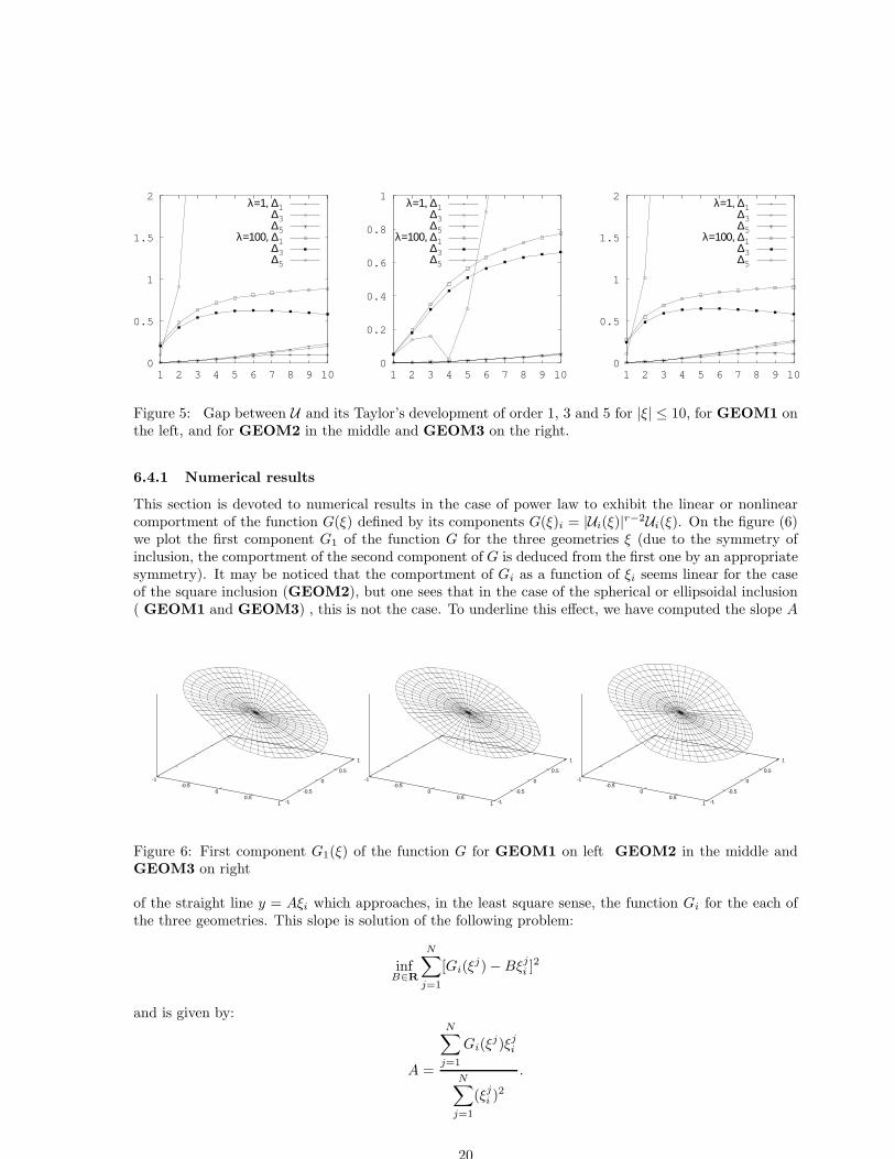
figures (3-4) the same quantities (eq. (99–101)) for a fixed direction of ξ and for length 0 ≤ |ξ| ≤ 1. Letconsider first figure (3) concerning GEOM1. In the case of λ1 = 1 one may see that for the range ofconsidered ξ, the filtration law is very close to Darcy’s law: the relatives errors, independently of order, aresmaller than 1%. But in the case of λ2 = 100, one needs the fifth approximation to obtain error smallerthan 1%. Secondly, when considering figure (4) concerning GEOM2, one may see that independentlyof the value of λ, the behaviour of U remains almost linear: for λ1 = 1 error is smaller than 0.8% andfor λ1 = 100 error is smaller than 8%. To close this numerical study of theoretical results concerningCarreau’s viscosity, we have computed solution of (21–24) and the different gaps (eq. (99–101)) for |ξ|larger than 1, to obtain numerical limit of validity of the Taylor’s expansion, for the three geometriesbut only for one fixed direction of ξ: 6 (e1, ξ) = 60. Those results are plotted on figure 5. One may seethat for the three geometries, Taylor’s expansions give good results for λ1 = 1 for the considered rangeof ξ, but in the case of larger parameter λ2 = 100 one loses precision of the Taylor’s expansion. Moreprecisely, the best results are for the third order Taylor’s expansion, but the fifth order expansion gives

18

0.004

0.005

0.006

0.007

0.008

0.009

0.01

0.20.30.40.50.60.70.80.9 1

∆1

∆3

∆5

0

0.05

0.1

0.15

0.2

0.25

0.3

0.20.30.40.50.60.70.80.9 1

∆1

∆3

∆5

Figure 3: Gap between U and its Taylor’s expansion for GEOM1:|ξ| ≤ 1, (e1, ξ) = 45, λ = 1 on theleft, λ = 100 on the right.

0.004

0.005

0.006

0.007

0.008

0.009

0.01

0.20.30.40.50.60.70.80.9 1

∆1

∆3

∆5

0

0.02

0.04

0.06

0.08

0.1

0.20.30.40.50.60.70.80.9 1

∆1

∆3

∆5

Figure 4: Gap between U and its Taylor’s expansion for GEOM2:|ξ| ≤ 1, (e1, ξ) = 45, λ = 1 on theleft, λ = 100 on the right.

very bad results ( the rest of the Taylor expansion of order 7 becomes non negligible). This suggests thatfor large |ξ| and λ the Taylor’s series diverge.

6.4 Numerical simulation for Power viscosity law

In this section, we propose to solve (21–24) for a sampling of ξ when viscosity is governed by a Powerlaw to illustrate the theoretical results of section 4. At first, we describe parameters of the Power lawand the numerical experiments procedure. Due to the homogeneity property of the power law viscosity,we just consider a viscositiy law with λ = 1. We chose arbitrarely a flow index r = 1.5 :

η(e(u)) = |e(u)|−.5

For the same reason of homogeneity, we consider only the solution of the nonlinear problem (21–24) for|ξ| = 1. Numerical solution are performed for a sampling ξj of ξ defined by:

ξj = t(cosjπ

4m, sin

jπ

4m), 0 ≤ j ≤ m = 8 (102)

and any extended by symmetry as in the Carreau’s case. In two following sections, we will numericallyshow the different behaviour of the filtration law depending on the geometry of porous medium.

19

0

0.5

1

1.5

2

1 2 3 4 5 6 7 8 9 10

λ=1, ∆1

∆3

∆5

λ=100, ∆1

∆3

∆5

0

0.2

0.4

0.6

0.8

1

1 2 3 4 5 6 7 8 9 10

λ=1, ∆1

∆3

∆5

λ=100, ∆1

∆3

∆5

0

0.5

1

1.5

2

1 2 3 4 5 6 7 8 9 10

λ=1, ∆1

∆3

∆5

λ=100, ∆1

∆3

∆5

Figure 5: Gap between U and its Taylor’s development of order 1, 3 and 5 for |ξ| ≤ 10, for GEOM1 onthe left, and for GEOM2 in the middle and GEOM3 on the right.

6.4.1 Numerical results

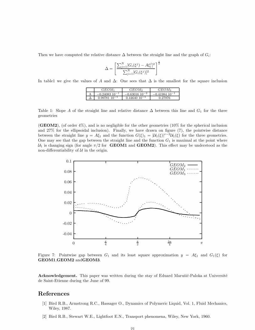
This section is devoted to numerical results in the case of power law to exhibit the linear or nonlinearcomportment of the function G(ξ) defined by its components G(ξ)i = |Ui(ξ)|r−2Ui(ξ). On the figure (6)we plot the first component G1 of the function G for the three geometries ξ (due to the symmetry ofinclusion, the comportment of the second component of G is deduced from the first one by an appropriatesymmetry). It may be noticed that the comportment of Gi as a function of ξi seems linear for the caseof the square inclusion (GEOM2), but one sees that in the case of the spherical or ellipsoidal inclusion( GEOM1 and GEOM3) , this is not the case. To underline this effect, we have computed the slope A

-1-0.5

00.5

1 -1

-0.5

0

0.5

1

-1-0.5

00.5

1 -1

-0.5

0

0.5

1

-1-0.5

00.5

1 -1

-0.5

0

0.5

1

Figure 6: First component G1(ξ) of the function G for GEOM1 on left GEOM2 in the middle andGEOM3 on right

of the straight line y = Aξi which approaches, in the least square sense, the function Gi for the each ofthe three geometries. This slope is solution of the following problem:

infB∈R

N∑

j=1

[Gi(ξj) − Bξj

i ]2

and is given by:

A =

N∑

j=1

Gi(ξj)ξj

i

N∑

j=1

(ξji )

2

.

20

Then we have computed the relative distance ∆ between the straight line and the graph of Gi:

∆ =

[

∑Nj=1[Gi(ξ

j) − Aξji ]

2

∑Nj=1[Gi(ξj)]2

]1

2

In table1 we give the values of A and ∆: One sees that ∆ is the smallest for the square inclusion

GEOM1 GEOM2 GEOM3

A −0.24083 10−1−0.63016 10−2

−0.41984 10−1

∆ 0.99781 10−1 0.44640 10−1 0.27976

Table 1: Slope A of the straight line and relative distance ∆ between this line and G1 for the threegeometries

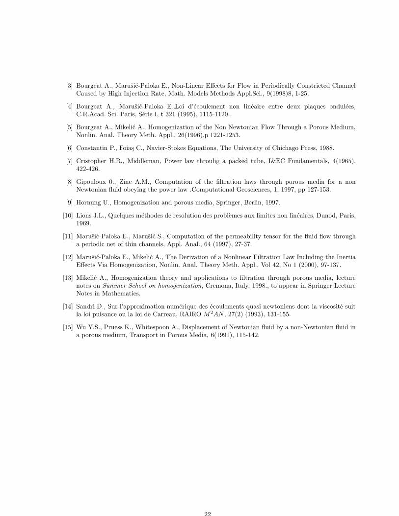
(GEOM2), (of order 4%), and is no negligible for the other geometries (10% for the spherical inclusionand 27% for the ellipsoidal inclusion). Finally, we have drawn on figure (7), the pointwise distancebetween the straight line y = Aξ1 and the function G(ξ)1 = |U1(ξ)|r−2U1(ξ) for the three geometries.One may see that the gap between the straight line and the function G1 is maximal at the point whereU1 is changing sign (for angle π/2 for GEOM1 and GEOM2). This effect may be understood as thenon-differentiability of U in the origin.

-0.04

-0.02

0

0.02

0.04

0.06

0.08

0.1

0π4

π2

3π4

π

GEOM2GEOM1GEOM3

Figure 7: Pointwise gap between G1 and its least square approximation y = Aξ1 and G1(ξ) forGEOM1,GEOM2 andGEOM3.

Acknowledgement. This paper was written during the stay of Eduard Marusic-Paloka at Universitede Saint-Etienne during the June of 99.

References

[1] Bird R.B., Armstrong R.C., Hassager O., Dynamics of Polymeric Liquid, Vol. 1, Fluid Mechanics,Wiley, 1987.

[2] Bird R.B., Stewart W.E., Lightfoot E.N., Transport phenomena, Wiley, New York, 1960.

21

[3] Bourgeat A., Marusic-Paloka E., Non-Linear Effects for Flow in Periodically Constricted ChannelCaused by High Injection Rate, Math. Models Methods Appl.Sci., 9(1998)8, 1-25.

[4] Bourgeat A., Marusic-Paloka E.,Loi d’ecoulement non lineaire entre deux plaques ondulees,C.R.Acad. Sci. Paris, Serie I, t 321 (1995), 1115-1120.

[5] Bourgeat A., Mikelic A., Homogenization of the Non Newtonian Flow Through a Porous Medium,Nonlin. Anal. Theory Meth. Appl., 26(1996),p 1221-1253.

[6] Constantin P., Foias C., Navier-Stokes Equations, The University of Chichago Press, 1988.

[7] Cristopher H.R., Middleman, Power law throuhg a packed tube, I&EC Fundamentals, 4(1965),422-426.

[8] Gipouloux 0., Zine A.M., Computation of the filtration laws through porous media for a nonNewtonian fluid obeying the power law .Computational Geosciences, 1, 1997, pp 127-153.

[9] Hornung U., Homogenization and porous media, Springer, Berlin, 1997.

[10] Lions J.L., Quelques methodes de resolution des problemes aux limites non lineaires, Dunod, Paris,1969.

[11] Marusic-Paloka E., Marusic S., Computation of the permeability tensor for the fluid flow througha periodic net of thin channels, Appl. Anal., 64 (1997), 27-37.

[12] Marusic-Paloka E., Mikelic A., The Derivation of a Nonlinear Filtration Law Including the InertiaEffects Via Homogenization, Nonlin. Anal. Theory Meth. Appl., Vol 42, No 1 (2000), 97-137.

[13] Mikelic A., Homogenization theory and applications to filtration through porous media, lecturenotes on Summer School on homogenization, Cremona, Italy, 1998., to appear in Springer LectureNotes in Mathematics.

[14] Sandri D., Sur l’approximation numerique des ecoulements quasi-newtoniens dont la viscosite suitla loi puisance ou la loi de Carreau, RAIRO M2AN , 27(2) (1993), 131-155.

[15] Wu Y.S., Pruess K., Whitespoon A., Displacement of Newtonian fluid by a non-Newtonian fluid ina porous medium, Transport in Porous Media, 6(1991), 115-142.

22