Turbulent mixing and chemical reaction in baffled ... - CORE

New Jersey Institute of TechnologyDigital Commons @ NJIT

Dissertations Theses and Dissertations

Summer 2000

Turbulent mixing and chemical reaction in baffledstirred tank reactors : a comparison betweenexperiments and a novel micromixing-basedcomputational fluid dynamics modelOtute AkitiNew Jersey Institute of Technology

Follow this and additional works at: https://digitalcommons.njit.edu/dissertations

Part of the Chemical Engineering Commons

This Dissertation is brought to you for free and open access by the Theses and Dissertations at Digital Commons @ NJIT. It has been accepted forinclusion in Dissertations by an authorized administrator of Digital Commons @ NJIT. For more information, please [email protected].

Recommended CitationAkiti, Otute, "Turbulent mixing and chemical reaction in baffled stirred tank reactors : a comparison between experiments and a novelmicromixing-based computational fluid dynamics model" (2000). Dissertations. 420.https://digitalcommons.njit.edu/dissertations/420

https://digitalcommons.njit.edu?utm_source=digitalcommons.njit.edu%2Fdissertations%2F420&utm_medium=PDF&utm_campaign=PDFCoverPages

https://digitalcommons.njit.edu/dissertations?utm_source=digitalcommons.njit.edu%2Fdissertations%2F420&utm_medium=PDF&utm_campaign=PDFCoverPages

https://digitalcommons.njit.edu/etd?utm_source=digitalcommons.njit.edu%2Fdissertations%2F420&utm_medium=PDF&utm_campaign=PDFCoverPages

https://digitalcommons.njit.edu/dissertations?utm_source=digitalcommons.njit.edu%2Fdissertations%2F420&utm_medium=PDF&utm_campaign=PDFCoverPages

http://network.bepress.com/hgg/discipline/240?utm_source=digitalcommons.njit.edu%2Fdissertations%2F420&utm_medium=PDF&utm_campaign=PDFCoverPages

https://digitalcommons.njit.edu/dissertations/420?utm_source=digitalcommons.njit.edu%2Fdissertations%2F420&utm_medium=PDF&utm_campaign=PDFCoverPages

mailto:[email protected]

Copyright Warning & Restrictions

The copyright law of the United States (Title 17, United States Code) governs the making of photocopies or other

reproductions of copyrighted material.

Under certain conditions specified in the law, libraries and archives are authorized to furnish a photocopy or other

reproduction. One of these specified conditions is that the photocopy or reproduction is not to be “used for any

purpose other than private study, scholarship, or research.” If a, user makes a request for, or later uses, a photocopy or reproduction for purposes in excess of “fair use” that user

may be liable for copyright infringement,

This institution reserves the right to refuse to accept a copying order if, in its judgment, fulfillment of the order

would involve violation of copyright law.

Please Note: The author retains the copyright while the New Jersey Institute of Technology reserves the right to

distribute this thesis or dissertation

Printing note: If you do not wish to print this page, then select “Pages from: first page # to: last page #” on the print dialog screen

The Van Houten library has removed some of the personal information and all signatures from the approval page and biographical sketches of theses and dissertations in order to protect the identity of NJIT graduates and faculty.

ABSTRACT

TURBULENT MIXING AND CHEMICAL REACTION IN BAFFLED STIRRED TANKREACTORS: A COMPARISON BETWEEN EXPERIMENTS AND A NOVELMICROMIXING-BASED COMPUTATIONAL FLUID DYNAMICS MODEL

byOtute Akiti

The optimization of reaction processes to maximize the yield of a desired product while

minimizing the formation of undesired by-products is one of the most important steps in

process development for drug manufacturing or fine chemical production. In many situ-

ations the kinetics of product formation can be quite complex and involve a number of

intermediate steps as well as parallel and serial reactions. This renders the systems sensi-

tive to the operating conditions. Often, upon scale-up, a decrease in the yield of the desired

product is experienced, while more undesired by-products are produced. A large number of

interrelated variables influence the outcome of a process, and furthermore, most systems of

process interest take place under turbulent conditions. Present methods for process design

are inadequate because they involve the use of lumped parameters which fail to capture

essential flow details and the rapid changes in the local concentration of reactants.

In recent years Computational Fluid Dynamics (CFD) has been successfully used to

model the fluid dynamics of complex vessels (such as agitated reactors) and to predict

the velocity distribution in turbulent systems such as mixers and reactors. In this work

a novel approach based on the use of CFD coupled with micromixing models was used

to predict the behavior of a multiple, competitive reaction system in cylindrical stirred

tank reactors fitted with a variety of agitators. In particular, the following fast parallel

competing reactions scheme (Bourne and Yu 1994) was modeled, and the results compared

with original experimental data:

The reactor was operated in semi-batch mode, with the limiting reagent (A) being slowly

added to the contents of the reactor in which the other reagents (B and C) were already

dissolved. The final yield of the undesired product (S) was experimentally measured. The

flow field in the reactor was simulated using the Reynolds Stress (RSM) turbulence model.

The full impeller geometry was incorporated in the CFD simulation using the Multiple

Reference Frames (MRF) model. The reaction zone was modeled in a Lagrangian way

using a multi-phase Volume of Fluid (VOF) model (Hirt and Nichols 1981). The interaction

of turbulence and reaction was accounted for by means of the engulfment-based models

for micro-mixing (Baldyga and Bourne 1989a; Baldyga and Bourne 1989b; Baldyga et al . .

1997).

The agreement between experimental velocity distribution data and the results of the

simulations was generally good. The micro-mixing models, in conjunction with CFD,

predicted a final yield in close agreement with the experimental data, demonstrating that

the proposed approach can be successfully used to model turbulent reactive systems without

the need for experimental input.


byOtute Akiti

A DissertationSubmitted to the Faculty of

New Jersey Institute of Technologyin Partial Fulfillment of the Requirements for the Degree of

Doctor of Philosophy in Chemical Engineering

Department of Chemical Engineering, Chemistry, and Environmental Science

August 2000

APPROVAL PAGE


Otute Akiti

Dr. Piero M. Armenante, Dissertation Director DateProfessor of Chemical Engineering, NJIT

Dr. Cordon Lewandowski, Committee Member DateDistinguished Professor of Chemical Engineering, NJIT

Dr. Robert Barat, Committee Member DateAssociate Professor of Chemical Engineering, NJIT

Dr. ;Norman Loney, Committee Member DateAssociate Professor of Chemical Engineering, NJIT

Dr. Pushpendra Singh, Committee Member DateAssistant Professor of Mechanical Engineering, NJIT

BIOGRAPHICAL SKETCH

Author: Otute Akiti

Degree: Doctor of Philosophy in Chemical Engineering

Date: August 2000

Undergraduate and Graduate Education:

• Doctor of Philosophy in Chemical Engineering,New Jersey Institute of Technology, Newark, New Jersey, 2000

• Master of Science in Chemical Engineering,Northeastern University, Boston, Massachusetts, 1995

• Bachelor of Science in Chemical Engineering,University of California at Berkeley, Berkeley, California, 1993

Major: Chemical Engineering

Presentations and Publications:

Otute Akiti and Piero M. Armenante, "A Computational and Experimental Study of Mixingand Chemical Reaction in a Stirred Tank Reactor Equipped with a Down-pumpingHydrofoil Impeller using a Micro-Mixing-Based CFD Model." Proceedings of the10th European Conference on Mixing, Delft, The Netherlands, July 2-5,2000.

Otute Akiti and Piero M. Armenante, "Mixing and Reaction in a Baffled Stirred Tank Re-actor: A study of the Effects of Varying Viscosity on Mixing Sensitive ReactionsUsing a Novel Micro-Mixing Based CFD Model." Annual Meeting of the AmericanInstitute of Chemical Engineers, Dallas Texas, November 1999.

Otute Akiti and Piero M. Armenante, "A Computational and Experimental Study of Mixingand Reaction in Stirred Tank Reactors using a Novel Micro-Mixing-Based Model"Annual Meeting of the American Institute of Chemical Engineers, Dallas Texas,November 1999.

Otute Akiti and Piero M. Armenante, "Mixing and Reaction in a Baffled Stirred Tank Re-actor. Comparison Between Experiments and a Novel Micromixing Based CFDModel" 17th Biennial North American Mixing Conference, Banff, Alberta, Canada,August 15-20 1999.

iv

Akiti et al, "Multiphasic or 'Pulsatile' Controlled Release System for the Delivery of Vac-cines", in Human Biomaterials Applications, Humana Press Inc., 1996.

To my family

vi

ACKNOWLEDGMENT

I would like to take this opportunity to say a few words of thanks to those who supported

me and were instrumental in bringing this work to fruition.

I would firstly of like to thank my advisor, Professor Armenante, for his guidance and

support during this project. He was not just a good advisor, but also a good teacher and I

have benefitted tremendously from his excellent advice over the course of my studies here

at NJIT.

I would also like express my sincere thanks to Dr. Gordon Lewandowski, Dr. Norman

Loney, Dr. Robert Barat and Dr. Pushpendra Singh for serving as Committee Members.

A special thanks goes to Clint Brockway for his invaluable assistance with analytical

laboratory equipment, and also to Larisa Krishtopa who filled in his big shoes after his

departure. I would also like to thank Yogesh Gandhi in the chemical stockroom for his

support. I would also like to thank Cindy Wos and Peggy Schel for their kind assistance

with administrative work in the department.

I would like to thank Dr. Lanre Oshinowo, Dr. Liz Marshall and the rest of the Fluent

support team for their technical assistance with using the Fluent CFD code.

This work was supported in part by a grant from the Emission Reduction Research

Center at NJIT, and in particular the research institutes of the Schering Plough Corporation

and the Bristol-Myers Squibb Corporation. Their support is gratefully acknowledged.

A special thanks to my friends here at NJIT, and the rest of the gang, who have con-

tributed to making my experience as a student a most enjoyable one.

I would like to thank my parents, my brother and my sister for their patience and sup-

port.

To all the above, and anyone who I may have missed, thank you.

vii

TABLE OF CONTENTS

Chapter Page

1 INTRODUCTION 11.1 Mixing in Industry and Research 11.2 Mixing and Chemical Reaction 2

1.2.1 The Mechanically Agitated Vessel 21.2.2 The Influence of Mixing on Chemical Reactions 2

1.3 Objective 11

2 THEORETICAL BACKGROUND 142.1 Mixing Sensitive Reaction System 142.2 Turbulent Reacting Flows 15

2.2.1 Overview 152.2.2 Literature Review 17

2.3 Micromixing Models 202.3.1 The Standard Engulfment Model 222.3.2 The Modified Engulfment Model 25

2.4 Remarks 26

3 NUMERICAL SIMULATION 273.1 Modeling the Turbulent Flow Field 27

3.1.1 Conservation Equations 273.1.2 Conservation Equations for Turbulent Flows 28

3.2 Boundary Conditions 313.2.1 Boundary Conditions at Walls and Surfaces 313.2.2 Boundary Conditions for the Agitator 313.2.3 Grid Generation 34

3.3 Determining the Power Imparted to the System 353.3.1 Power Number Correlation for the Rushton Turbine 373.3.2 Power Number Correlation for the Chemineer High Efficiency Im-

peller (HE-3) 383.3.3 Power Number Correlation for the 6 Blade Pitched-Blade Turbine 383.3.4 Evaluation of the Impeller Reynolds Number 38

3.4 Evaluation of Mixing Time 383.4.1 Mixing Time for the Rushton Turbine 383.4.2 Mixing Time for the Chemineer High Efficiency Impeller 393.4.3 Mixing Time for the 6 Blade Pitched Blade Turbine 39

3.5 A Novel Model Simulating Turbulent Reacting Flows 393.5.1 Model Formulation 40

3.6 Numerical Solution of the Micromixing Model Equations 45

viii

TABLE OF CONTENTS(Continued)

Chapter Page

3.6.1 Standard Engulfment Model 453.6.2 Modified Engulfment Model Equations 46

4 EXPERIMENTAL APPARATUS AND METHOD 474.1 Experimental Measurement of the Turbulent Flow Field 47

4.1.1 Experimental LDV Setup 474.1.2 Measurements Provided by LDV 51

4.2 Experimental Investigation of Power Draw 534.3 Experimental Investigation of Micro-mixing 55

5 RESULTS AND DISCUSSION 645.1 Reproducibility of Experimental Data 655.2 Effect of Feed Discretization of the Yield 65

5.2.1 Remarks 685.3 Results for Systems Al, A2, A3

Rushton Turbine: Impeller off Bottom Clearance C = T/3 705.3.1 System Configuration 705.3.2 Comparison of LDV Data with FLUENT CFD Simulations for

System Al 735.3.3 Comparison of LDV Data with FLUENT CFD Simulations for

System A2 795.3.4 Power Consumption 835.3.5 Comparison of Predicted Product Yields for System Al with Ex-

periment 835.3.6 Comparison of Predicted Product Yields for System A2 with Ex-

periment 885.3.7 Comparison of Predicted Product Yields for System A3 with Ex-

periment 905.3.8 Remarks 92

5.4 Results for Systems B1 and B2Pitched Blade Turbine: Impeller off Bottom Clearance C = T/3 965.4.1 System Configuration 965.4.2 Comparison of LDV Data with CFD Simulations for System B1 . 995.4.3 Comparison of LDV Data with CFD Simulations for System B2 . 1055.4.4 Remarks 1095.4.5 Power Consumption 1095.4.6 Comparison of Predicted Product Yields in Aqueous Medium with

the Model 1095.4.7 Comparison of Predicted Product Yields in Viscous Medium with

the Model 1145.4.8 Comparison of System B1 and System B2 123

ix

TABLE OF CONTENTS(Continued)

Chapter Page

5.4.9 Remarks 1235.5 Results for System C

Chemineer High Efficiency Impeller (HE-3): Impeller off Bottom Clear-ance C = T/3 1255.5.1 System Configuration 1255.5.2 Comparison of LDV Data with FLUENT CFD Simulations 1285.5.3 Power Consumption 1345.5.4 Remarks 1345.5.5 Comparison of Predicted Product Yields with the Model 1345.5.6 Remarks 139

5.6 Results for System DRushton Turbine: Impeller off Bottom Clearance C = T/2 1415.6.1 System Configuration 1415.6.2 Comparison of LDV Data with FLUENT CFD Simulations 1415.6.3 Remarks 1495.6.4 Power Consumption 1495.6.5 Comparison of Predicted Product Yields with the Model 1495.6.6 Effect of Impeller Off-bottom Clearance 153

6 CONCLUSION 157

APPENDIX A FORTRAN CODE USED IN THE EVALUATION OF THE MI-CROMIXING MODEL EQUATIONS 162A.1 Runge-Kutta Solver 162A.2 Driver Module 163A.3 Solver Module 167

REFERENCES 176

LIST OF TABLES

Table Page

1.1 Overview of the impellers used 91.2 Summary of systems under investigation 10

3.1 Summary of Grids Used 36

4.1 Summary of feed point locations 594.2 Feed Point Locations used for Each System 60

5.1 Power and mixing time results for systems A 1 and A2 845.2 Power and mixing time characteristics for Systems B1 and B2 1105.3 Power and mixing time results for System C 1355.4 Power and mixing time characteristics for System D 150

xi

LIST OF FIGURES

Figure Page

1.1 Typical arrangement for a mechanically agitated vessel 31.2 Reaction in a perfectly mixed environment 51.3 Reaction in a completely segregated environment 51.4 Outline of research work 13

2.1 A simplified depiction of turbulence in a mechanically agitated system. . 202.2 Principal stages of micromixing 222.3 Schematic representation of the E-Model 24

3.1 Illustration of the MRF model 333.2 Outline of Proposed Model 42

4.1 Details of impellers used 484.2 Laser Doppler Velocimetry fringe model 494.3 Laser Doppler Velocimetry apparatus 504.4 Position of the mixing vessel with respect to the laser assembly to measure

all the velocity components. 524.5 Experimental apparatus for the measurement of power draw. 544.6 Experimental apparatus for the investigation of fast competitive parallel

reactions. 564.7 Feed point locations 584.8 Schematic representation of how t, varies with feed time 60

5.1 Effect of feed discretization on yield: System D, 100rpm 665.2 Effect of feed discretization on yield: System D, 300rpm 665.3 Effect of feed discretization on yield: System B 1, 100 rpm 675.4 Effect of feed discretization on yield: System Bl, 400 rpm 675.5 Effect of feed discretization on yield: System C, 400 rpm 685.6 Effect of feed discretization on yield: System C, 400 rpm 695.7 Stirred tank equipped with a Rushton turbine at an impeller clearance of

T/3: Locations where LDV data was taken. 715.8 Stirred tank equipped with a Rushton turbine at an impeller clearance of

T/3: Outline grid 725.9 Stirred tank equipped with a Rushton turbine at an impeller clearance of

T/3: Outline grid showing mesh details. 725.10 Stirred tank equipped with a Rushton turbine at an impeller clearance of

T/3: Average velocity profile. 745.11 Stirred tank equipped with a Rushton turbine at an impeller clearance of

T/3: Comparison of experimental axial velocity data with CFD simulation 75

xii

LIST OF FIGURES(Continued)

Figure Page

5.12 Stirred tank equipped with a Rushton turbine at an impeller clearance ofT/3: Comparison of experimental radial velocity data with CFD simulation. 76

5.13 Stirred Tank equipped with a Rushton turbine at an impeller clearance ofT/3: Comparison of experimental tangential velocity data with CFD simu-lation. 77

5.14 Stirred Tank Equipped with a Rushton Turbine at an Impeller Clearanceof T/3: Comparison of Experimental Turbulent Kinetic Energy Data withCFD Simulation. 78

5.15 Stirred Tank Equipped with a Rushton turbine at an impeller clearance ofT/3: Comparison of experimental axial velocity data with CFD simulationin viscous medium 79

5.16 Stirred tank equipped with a Rushton turbine at an impeller clearance ofT/3: Comparison of experimental radial velocity data with CFD simulationin viscous medium 80

5.17 Stirred tank equipped with a Rushton turbine at an impeller clearance ofT/3: Comparison of experimental tangential velocity data with CFD simu-lation in viscous medium. 81

5.18 Stirred Tank equipped with a Rushton turbine at an impeller clearance ofT/3: Comparison of experimental turbulent kinetic energy data with CFDsimulation in viscous medium. 82

5.19 Reaction profile for system Al at 100rpm. Feed location Fs. 855.20 Reaction profile for System Al at 300rpm. Feed location Fs. 865.21 Reaction zone trajectory. System Al, feed near liquid surface at 200rpm. . 875.22 Variation of product yield with agitation speed for System Al. Feed loca-

tion Fs. 885.23 Reaction time for System A2 at 100rpm. Feed location Fs. 905.24 Reaction time for System A2 at 300rpm. Feed location Fs. 915.25 Variation of product yield with agitation speed for System A2. Feed loca-

tion Fs. 925.26 Variation of product yield with feed time for System A3 935.27 Reaction profile for System A2 at 100rpm. Feed location Fs. 935.28 Reaction profile for System A3 at 300rpm. Feed location Fs. 945.29 Variation of Product Yield with Agitation Speed for System A3. Feed Lo-

cation Fs. 955.30 Stirred tank equipped with a pitched blade turbine at an impeller clearance

of T/3: Locations where LDV data was taken 975.31 Stirred tank equipped with a pitched blade turbine at an impeller clearance

of T/3: Outline grid. 985.32 Stirred tank equipped with a pitched blade turbine at an impeller clearance

of T/3: Outline grid showing mesh details 98


Figure Page

5.33 Stirred tank equipped with a pitched blade turbine at an impeller clearanceof T/3: Velocity profile 100

5.34 Stirred tank equipped with a pitched blade turbine at an impeller clearanceof T/3: Comparison of experimental axial velocity data with CFD simulation.101

5.35 Stirred tank equipped with a pitched blade turbine at an impeller clearanceof T/3: Comparison of experimental radial velocity data with CFD simulation.102

5.36 Stirred tank equipped with a pitched blade turbine at an impeller clearanceof T/3: Comparison of experimental tangential velocity data with CFD sim-ulation. 103

5.37 Stirred Tank Equipped with a Pitched Blade Turbine at an Impeller Clear-ance of T/3: Comparison of Experimental Turbulent Kinetic Energy Datawith CFD Simulation. 104

5.38 Stirred tank equipped with a pitched blade turbine at an impeller clearanceof T/3: Comparison of experimental axial velocity data with CFD simula-tion in viscous medium. 105

5.39 Stirred tank equipped with a pitched blade turbine at an impeller clearanceof T/3: Comparison of experimental radial velocity data with CFD simula-tion in viscous medium. 106

5.40 Stirred tank equipped with a pitched blade turbine at an impeller clearanceof T/3: Comparison of experimental tangential velocity data with CFD sim-ulation in viscous medium 107

5.41 Stirred tank equipped with a pitched blade turbine at an impeller clear-ance of T/3: Comparison of experimental turbulent kinetic energy data withCFD simulation in viscous medium. 108

5.42 Variation of Product Yield with Feed Time for System Bl. Feed Location Fs.1115.43 Reaction time for system B1 at 100rpm. Feed location Fs. 1125.44 Reaction time for system B1 at 100rpm. Feed location Fi. 1125.45 Reaction time for system B1 at 400rpm. Feed location Fs. 1135.46 Reaction time for system B1 at 400rpm. Feed location Fi. 1135.47 Reaction zone trajectory. System B 1, feed near surface, 400rpm 1155.48 Reaction zone trajectory. System B 1, feed above impeller, 400rpm 1165.49 Variation of Product Yield with Agitation Speed for System B 1. Feed Lo-

cation Fs. 1175.50 Variation of Product Yield with Agitation Speed for System Bl. Feed Lo-

cation Fs2. 1185.51 Variation of Product Yield with Agitation Speed for System B 1. Feed Lo-

cation Fi. 1185.52 Variation of Product Yield with Feed Time for System B2 1195.53 Reaction time for system B2 at 100rpm. Feed location Fs. 1195.54 Reaction time for system B2 at 100rpm. Feed location Fi 1205.55 Reaction time for system B2 at 400rpm. Feed location Fs. 120

xiv


Figure Page

5.56 Reaction time for system B2 at 400rpm. Feed location Fi 1215.57 Variation of Product Yield with Agitation Speed for System B2. Feed Lo-

cation Fs 1225.58 Variation of Product Yield with Agitation Speed for System B2. Feed Lo-

cation Fs. 1235.59 Comparison of System B1 and System B2: Feed location Fs 1245.60 Stirred tank equipped with a Chemineer High Efficiency impeller at a clear-

ance of T/3: Locations where LDV data was taken. 1265.61 Stirred Tank Equipped with a Chemineer High Efficiency Impeller at an

impeller clearance of T/3: Outline grid. 1275.62 Stirred tank equipped with a Chemineer High Efficiency impeller at an

impeller clearance of T/3: Outline grid showing mesh details. 1275.63 Stirred Tank Equipped with a Chemineer High Efficiency Impeller at an

impeller clearance of T/3: Velocity profile. 1295.64 Stirred Tank equipped with a Chemineer High Efficiency impeller at an

impeller clearance of T/3: Comparison of experimental axial velocity datawith CFD simulation 130

5.65 Stirred tank equipped with a Chemineer High Efficiency impeller at animpeller clearance of T/3: Comparison of experimental radial velocity datawith CFD simulation 131

5.66 Stirred tank equipped with a Chemineer High Efficiency impeller at animpeller clearance of T/3: Comparison of experimental tangential velocitydata with CFD simulation. 132

5.67 Stirred Tank Equipped with a Chemineer High Efficiency Impeller at anImpeller Clearance of T/3: Comparison of Experimental Turbulent KineticEnergy Data with CFD Simulation. 133

5.68 Variation of Product Yield with Feed Time for the HE-3 1365.69 Reaction profile for system C at 100rpm. Feed location Fs. 1375.70 Reaction profile for system C at 100rpm. Feed location Fi. 1375.71 Reaction time for system C at 400rpm. Feed location Fs. 1385.72 Reaction time for system C at 400rpm. Feed location Fi. 1385.73 Variation of by-product yield with agitation speed for the HE-3. Feed loca-

tion Fs 1395.74 Variation of by-product yield with agitation speed for the HE-3. Feed loca-

tion Fi. 1405.75 Stirred tank equipped with a Rushton turbine at an impeller clearance of

T/2: Locations where LDV data was taken. 1425.76 Stirred tank equipped with a Rushton turbine at an impeller clearance of

T/2: Outline grid 1435.77 Stirred Tank equipped with a Rushton turbine at an impeller clearance of

T/2: Outline grid showing mesh details. 143

xv


Figure Page

5.78 Stirred tank equipped with a Rushton turbine at an impeller clearance ofT/2: Velocity profile. 144

5.79 Stirred tank equipped with a Rushton turbine at an impeller clearance ofT/2: Comparison of experimental axial velocity data with CFD simulation 145

5.80 Stirred tank equipped with a Rushton turbine at an impeller Clearance ofT/2: Comparison of experimental radial velocity data with CFD simulation. 146

5.81 Stirred tank equipped with a Rushton turbine at an impeller clearance ofT/2: Comparison of experimental tangential velocity data with CFD simu-lation. 147

5.82 Stirred tank equipped with a Rushton turbine at an impeller clearance ofT/2: Comparison of experimental turbulent kinetic energy data with CFDsimulation. 148

5.83 Variation of product yield with feed time for System D 1515.84 Reaction profile for System D at 100rpm. Feed location Fs 1525.85 Reaction profile for System D at 100rpm. Feed location Fi 1525.86 Reaction profile for System D at 300rpm. Feed location Fs 1535.87 Variation of product yield with feed time for System D at 300rpm. Feed

location Fi. 1545.88 Variation of product yield with agitation speed for System D. Feed Location

Fs 1545.89 Variation of product yield with agitation speed for System D. Feed location

Fi 1555.90 Variation of product yield with agitation speed for System D. Feed location

Fd 1555.91 Effect of increasing the impeller off-bottom clearance: Comparing System

A3 and System D 156

xvi

NOMENCLATURE

Symbol Variable Units

A Impeller blade angle radiansC Impeller clearance off vessel bottom mCi Concentration of species i moles IndC i Average concentration of speciesi moles /m3

CZ Fluctuating concentration of species i moles I m3

D Impeller Diameter mDk Mass diffusivity of species k Tn2 1 s

E Engulfment rate 1/sFi External force N (N ewtons)H Liquid height m

Jk,i Mass flux of species k kgm2 IsN Impeller speed rev/sNpo Impeller power number —P Pressure Pa(Pascals)Po Power dissipated by impeller WattsR Vessel Radius mRi Reaction source term —Sc Schmidt number —T Tank diameter M

Utip Impeller tip velocity m/sU Degree of Mixing —✓ Vessel Volume m,3Vet Engulfment volume m,3V, Initial dispersed phase volume m,3Xs Yield of species S —Cp Specific heat J I mol • kgknKinetic rate constant for reaction n m3 I mol • snb Number of Impeller Blades —t Time sui Velocity vector m/sui Average velocity vector m/s74 Fluctuating velocity vector m/su, Axial velocity m/sv, Radial velocity m/swv Tangential velocity m/sxi Cartesian coordinate components mZ Vessel liquid height m,z Axial location in vessel m

xvii

NOMENCLATURE

Greek Symbols Variable (Continued) Units

k Kronecker delta —

E Turbulent energy dissipation rate m2/s3

E• 'kz3 Alternating unit tensor --lc Turbulent kinetic energy n2/s2

,u, Molecular viscosity Pa • s

Pt Turbulent viscosity Pa • slief f Effective viscosity (fi t + ii,) Pa • sv Kinematic viscosity M2/sq5 Mass fraction of species k —

Pk Mass density kg /T113

Pk Mass density of phase k kg/m3a Number of times feed is discretized —

Omix Mixing time s

T Torque N (Newtons)Q Rotating speed of reference frame rad/sw Impeller speed rad/s

xviii

CHAPTER 1

INTRODUCTION

1.1 Mixing in Industry and Research

Mixing processes are part of the infrastructure of the Chemical Process Industries (CPI).

Mixing operations are encountered in industries such as: specialty chemicals, biotechnol-

ogy, pharmaceutical, environmental (wastewater treatment), petroleum and polymer indus-

tries, to name a few, and serve to bring together the various process streams into contact

to achieve desired objectives. These objectives include: the acceleration of heat transfer as

a means of controlling temperature, the blending of liquids (homogenization), separation

processes (e.g. solvent extraction), crystallization, and chemical reactions. Consequently,

practically every plant contains a mixing process of some sort (Hamby et al. 1985).

As a result of their importance, mixing operations have been the subject of considerable

study, and significant literature exists on the subject with the aim of furnishing design

principles for many situations of industrial significance.

Economic losses that are incurred as a result of poor mixing are significant. In the

United States alone, the output value from the chemical process industries is estimated at

$750 billion (Tatterson et al. 1991). It is estimated that mixing related problems account for

losses anywhere from 0.5 % to 3 % of that total. This translates into $1 billion—$20 billion

in losses each year. In industries such as the pharmaceutical industry where the products

require expensive reagents, are produced in relatively small quantities, and must meet ex-

ceptionally high purity standards, the losses are even more spectacular and may represent

up 10 % of the turnover (Tatterson et al. 1991; Leng 1991; Smith 1990).

Despite their importance, mixing processes are still not well understood. This work fo-

cuses on addressing the problems that arise when mixing operations influence the outcome

of chemical reactions.

1

2

1.2 Mixing and Chemical Reaction

1.2.1 The Mechanically Agitated Vessel

Because mixing operations cover a diverse spectrum of industries and applications, the

equipment used for the purpose of mixing are equally diverse and include: mechanically

agitated vessels, jet mixers, static mixers, extruders and mills.

This work focuses on the mechanically agitated tank, or stirred tank. The agitated

vessel or stirred tank is widely used in the chemical process industries to effect mixing,

especially where there is a need to maintain constant temperature and composition. The

mechanical agitated vessel is typically a cylindrical vessel filled to some depth with the

liquid of interest. The base of the tank may be flat, conical or spherical depending on

the application. Baffles are included to prevent vortexing behavior when working with

low viscosity liquids. The impeller is the device used to induce mixing. One more more

impellers may be used. The impeller is generally mounted on a shaft which is driven by a

motor. Heat transfer is effected by means of an external jacket or an internal cooling coil,

or both. A schematic of a typical stirred tank is shown in Figure 1.1.

1.2.2 The Influence of Mixing on Chemical Reactions

This work focuses on mixing operations in batch stirred tank reactors (BSTR) with slow

feed addition where reactions that are characterized as being "fast" and "complex", are

taking place. In the BSTR one or several feed streams to the vessel are present while no

exit streams are present. The BSTR is commonly encountered in industrial practice, and

in particular the pharmaceutical industry. Such a reactor allows the control of temperature

and helps prevent "runaway" reactions.

A "fast" reaction system, in the context of this work, refers to a system where the

reaction time is on the order of magnitude, or shorter, than the time it would take to ho-

mogenize the contents of the mixing tank (blending time). This has important implications

Figure 1.1: Typical arrangement for a mechanically agitated vessel.

4

when "complex" reactions are involved.

A "complex" reaction system in this context is one where several interrelated reactions

are taking place. An example of a complex reaction system would be a parallel competing

reaction system of the following type:

where k 1 k2 and reactant A may react via two possible pathways.

Such a reaction scheme is commonly encountered in practice where a main reaction

is taking place and unwanted side reactions are taking place alongside it. The unwanted

side reactions may use up valuable reactants, produce species that reduce the purity of the

desired product, or produce species that necessitate additional downstream processing steps

in order to meet product specifications. This reduces the overall efficiency of the process.

When the reactions occurring are "fast", the reactants will be consumed before the

contents of the mixing vessel are homogenized. In the example shown by Equations 1.1

and 1.2, this means that different amounts of Products P and S will be produced depending

on the local environment Reactant A experiences. The manner in which this occurs is best

illustrated by considering two extreme possibilities: the the perfectly mixed system and the

the completely segregated system.

In a perfectly mixed system, with an initial equimolar mixture of reactants A, B and

C, reactant A will "see" reactants B and C equally, and the final product distribution will

depend solely on the kinetics. Because the first reaction is much faster than the second,

k 1 k2, it will take place preferentially and little or no S product will form (Figure 1.2).

In a completely segregated system, where reactants B and C are segregated, and equal

amounts of all the reactants are present initially, the reactions take place independently of

each other such that reactant A sees both reactants B and C equally, and equal amounts of

products P and S form (Figure 1.3).

Figure 1.2: Reaction in a perfectly mixed environment

5

Figure 1.3: Reaction in a completely segregated environment

In a real system, where "fast" reactions are taking place, the system is neither in a

state of complete mixedness nor is it in a state of complete segregation, and intermediate

degrees of mixing are observed. This means that the kinetics as well as the hydrodynamics

will dictate the final product distribution.

Most mixing problems occur in the scale-up stage because the prevailing hydrody-

namics in large vessels is different from those in smaller ones where the processes are

developed. Mixing times in small vessels are typically small, and often smaller than the

characteristic reaction times; this means that reactions are more likely to take place in a

homogeneous environment. Mixing times in large vessels (such as industrial reactors) are

typically large. The mixing time in a 10,000 gallon reactor can easily exceed 10 minutes

(Coy 1996). This means that reactions in an industrial reactor are likely to take place in an

inhomogeneous environment when "fast" reactions are involved. Undesired by-products

caused by mixing-sensitive reactions are more likely to be formed in large vessels than in

small vessels even if the same reactions are considered. Over-designing rarely leads to a

6

better process. Successful prediction of the final product distribution upon scale-up will

depend on a good understanding of the hydrodynamics and its influence on the kinetics.

For a long time, the approach used to analyze complex mixing systems was based on

measurement and dimensional analysis. This involved the use of parameters such as: the

Power Number, which is a measure of the power consumed by an impeller; the Impeller

Reynolds Number which provides an indication of the level of turbulence in a reactor, and

so on. While these parameters are useful, they describe an average, or overall reactor

performance which, in many cases, masks inhomogeneities and gradients (concentrations,

mixing intensity, temperature) that are important in determining the efficiency of a process.

The lumping process wipes out the inhomogeneities and consequently leads to an erroneous

estimation of the final product distribution. The inadequacy of using lumped parameters to

designing systems when fast complex reactions were taking place was clearly demonstrated

by Bourne and Yu (Bourne and Yu 1991).

In order to avoid the limitations of lumped parameter models, distributed parameter

models based on actual system hydrodynamics must be used. This requires a more accu-

rate knowledge of the local properties within the flow field of the reaction vessel. This

involves gathering a huge amount of information that, in practice, cannot be obtained from

experimentation. The only viable means of obtaining the necessary information is through

numerical computation. In this work computational Fluid Dynamics (CFD) was employed

for that purpose.

Computational Fluid Dynamics is an approach that involves the numerical solution of

the the equations of motion (mass, momentum and energy) in a flow geometry of interest.

These equations, together with subsidiary equations pertinent to the problem at hand, com-

prise a flexible and powerful tool. Examples of subsidiary equations that can be used in

conjunction with CFD are:

• Equations for turbulence quantities

• Equations describing chemical species present in the flow

7

• Equations describing the dynamics of solid species, gas bubbles or other liquids dis-

persed in the flow domain

Computational Fluid Dynamics (CFD) has been successfully applied to model fluid flow

in a variety of systems including stirred tanks (Ranade and Joshi 1990b; Ranade and Joshi

1989b; Brucato et al. 1998; Kresta and Wood 1991; Armenante and Chou 1994; Armenante

et al. 1994).

The application of CFD to studying turbulent flow in batch stirred tank reactors where

chemical reactions are taking place is not straightforward and the literature on the subject

is sparse. In fact, CFD codes are unable to predict the product distribution in reactive

flows exhibiting "fast" and "complex" chemistry. This is a result of the fact that CFD

provides information about the local bulk fluid flow or macromixing, based on user defined

boundary conditions. Chemical reaction is a molecular level process and takes place on the

microscale which CFD does not resolve.

Micromixing models (Baldyga and Bourne 1989a; Baldyga and Bourne 1989b; Baldyga

and Bourne 1984b; Baldyga and Bourne 1984a; Baldyga and Bourne 1984c; Bakker and

van den Akker 1994; Bakker and van den Akker 1996) have been developed for purpose of

modeling the effect of mixing on chemical reactions at the molecular level. Micromixing

models do not contain any information about the bulk flow — the macromixing. A satis-

factory means of linking information about the fluid dynamics to the kinetics to predict the

outcome of complex reactive mixing systems is lacking in the literature.

Most work involving the computational modeling of mixing and chemical reaction,

in stirred tanks, is based on a network of zones formulation (David et al. 1992; Bourne

and Yu 1994; Wang and Mann 1992; Baldyga and Bourne 1988). Because this method

requires experimentally derived correlations to describe the fluid flow, it is inadequate for

investigating scale-up issues on novel systems. Work on modeling fast complex reaction

systems using CFD was recently presented (Bakker and van den Akker 1994; Bakker and

van den Akker 1996). The results reported were most encouraging. This method was,

8

however, unable to adequately predict the final product selectivities in all parts of the flow

domain.

In this work, the final product yield of fast parallel competing reactions was studied for

a variety of stirred tank configurations, all operated in semi-batch mode. A detailed de-

scription of the apparatus and method is presented in Chapter 4. An introductory overview

is presented here.

A baffled stirred tank reactor was chosen for the study. The tank used was a flat bot-

tomed cylindrical vessel having a diameter of 0.29 meters. The tank was filled with liquid

up to a level equal to the vessel diameter. Four baffles of width one tenth of the tank di-

ameter were equally spaced around the periphery of the tank. The impeller clearance, C,

defined as the distance between the bottom of the tank and the center line of the impeller

blades, was varied in some experiments. A variety of agitators were used. Different agi-

tators produce different circulation patterns and different distributions of turbulent energy

and dissipation for the same tank geometry. In this work the impellers used were:

• A radial flow impeller: Rushton Turbine

• An axial flow impeller: 6 Blade Pitched Blade Turbine (PBT) with the blades inclined

at 45° to the horizontal

• A fluid foil impeller: The Chemineer High Efficiency Impeller (HE-3)

The three impellers used cover the majority of impeller types used in industrial practice

for the agitation of low viscosity liquid systems. Schematic representations of the three

impellers are presented in Table 1.1.

The mode of operation for the reactor system was semi-batch mode with the limiting

reagent being slowly fed into the previously dissolved contents of the reaction vessel.

A summary of all the systems used for this work are presented in Table 1.2.

Studies were performed in both viscous and aqueous media in order to ascertain the

effects of fluid viscosity of the complex chemistry. All simulation work was validated

Table 1.1: Overview of the impellers used

9

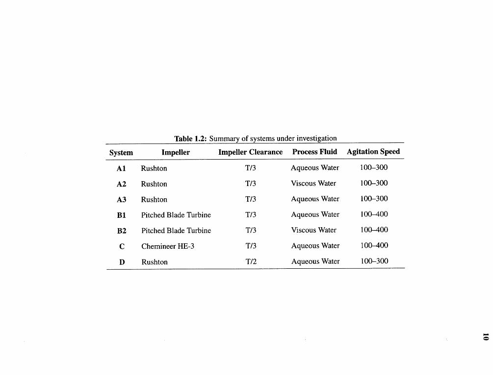
Table 1.2: Summary of systems under investigation

1 1

using original experimental data.

1.3 Objective

The overall objective of the present work was to develop a novel means of simulating

mixing and chemical reaction in batch stirred tank reactors by using existing models for

macromixing and micromixing as building blocks. A novel means of linking the various

building blocks of the problem is introduced so as to provide a general purpose tool that

can be used to predict the product distribution of fast complex reactions in BSTRs. All the

numerical tools used in this work were validated using original experimental data.

The issues that need to be tackled when modeling mixing and chemical reaction in

stirred tanks may be summarized as follows:

• An adequate description of the fluid flow in the geometry or interest

• An adequate description of the influence of turbulence on chemical reactions

• An adequate means of linking the description of the fluid flow with a mixing-sensitive

reaction model that accounts for molecular level phenomena to ultimately yield a

model that can be used to predict the course of fast complex reaction in stirred tanks.

The approach taken in this work to model the effects of mixing on complex reactions

systems in this work may be be outlined as follows:

• CFD was used to obtain a quantitative description of the flow in stirred tanks.

• A micromixing model was selected to predict the influence of mixing on chemical

reactions at the molecular level.

• A novel method to link macromixing and micromixing was used to successfully pre-

dict the product distribution of complex reaction systems.

12

• Original experimental work was conducted to collect data on the local fluid velocity

distribution for all the systems studied. The collected data was used to validate the

numerical predictions.

• Original experimental work was also conducted to determine the yield of complex

parallel reactions under different operating conditions. These experimental results

were used to validate the numerical predictions.

An outline of the work is summarized in Figure 1.4.

The critical step in the process is the coupling between information furnished by CFD

and the information supplied by the micromixing models. The means for doing this is not

generally agreed upon in the open literature and models that accomplish the task satisfac-

torily for stirred tank reactors are lacking. Therefore specific the objective of this work

is to develop a new model that successfully couples CFD with micromixing models to

furnish a new tool that can be used for the design of BSTRs in which fast complex

reactions are taking place.

Figure 1.4: Outline of research work

CHAPTER 2

THEORETICAL BACKGROUND

2.1 Mixing Sensitive Reaction System

A parallel competitive reaction system that is sensitive to mixing effects (Baldyga and

Bourne 1989b; Bourne and Yu 1991; Bourne and Yu 1994) was used to investigate the

effect of mixing on chemical reactions. The reaction system is represented by Equation 2.1

and Equation 2.2. The first reaction (Equation 2.1) is an acid base neutralization reac-

tion between hydrochloric acid (HCl) and sodium hydroxide (NaOH). The second reaction

(Equation 2.2), involves the hydrolysis of an ester, ethyl-chloroacetate (C H2ClCO2C2H5).

The rate constant k 1 , for the first, faster, reaction is given by:

while the rate constant k2, for the second, slower (but still relatively fast) reaction, is given

by the following Arrhenius rate expression (Bourne and Yu 1991):

This set of reactions is the well known Bourne reaction system # 4 (Baldyga and Bourne

1989b; Fox 1992; Bourne and Yu 1994). It is a well studied and characterized fast parallel

competing reaction system. In this reaction scheme, component B, hydrochloric acid, and

component C, ethyl-chloroacetate, compete for component A, sodium hydroxide. It is a

well studied system because it is representative of reactions systems that are encountered in

chemical reaction engineering practice where in addition to the primary reaction of interest,

another competing reaction may also take place.

For this particular reaction set, the yield, Xs, of forming component S (undesired by-

product) per mole of A (limiting reagent) fed to the system is of interest. The yield, Xs,

14

15

is defined as the moles of undesired by product S produced per mole of limiting reagent A

fed to the system. It is expressed as follows in terms of the reaction products:

This yield varies depending on the system hydrodynamics as is explained below.

When the mixing is perfect (no segregation exists), the final yield Xs , is dictated solely

by the kinetics and is given by:

For the above systems of equations, Xs is practically zero because k 1 >> k2 .

When the segregation is intense (the reactions take place independently of each other),

the yield becomes independent of the kinetics and is given by:

In the case where equal quantities of A, B and C are reacted, Xs = 0.5. Intermediate

degrees of mixing yields results between these two extremes and a means of evaluating the

state of mixing on the reaction kinetics is necessary.

2.2 Turbulent Reacting Flows

2.2.1 Overview

The process of turbulent mixing is extremely complex, largely because it involves a wide

range of time and length scales. Mixing is initiated at the macroscale level and proceeds

in a cascade like manner down to the microscale level. The macroscale level is important

because it is the source of the mixing process. Chemical reactions, however, can only take

place when the reacting species come into contact at the molecular level, the microscale

level (Fox 1996; Baldyga and Pohorecki 1998; Bourne 1993; Villermaux and Falk 1996;

16

Bourne and Baldyga 1999). These scales and all those in between must be accounted for

when modeling turbulent reacting flows.

For applications of chemical engineering interest, it is impossible to include a detailed

description of all relevant turbulence scales into a CFD code, in particular those scales that

take place at the sub-grid or molecular level, because the computational grid used for CFD

calculations does not, and cannot extend down to such a fine scale. A computational grid

used to describe a real physical system that contains a grid fine enough to resolve molecular

scale phenomena would require computer resources that are well beyond the capacity of

current computers. Furthermore, even with the present pace of computer development, this

will not be possible in the foreseeable future.

Thus molecular level phenomena such as micromixing, molecular diffusion, and chem-

ical reaction, must be modeled. The process of modeling can introduce significant simplifi-

cations into the physical description of the flow. In order to formulate acceptable algorithms

for reacting flows, one must first understand and properly address the complex interactions

between turbulence, molecular diffusion and chemical kinetics. At the very least, the fol-

lowing steps must be considered:

• Modeling the turbulence field in sufficient detail to resolve the rate controlling steps

of turbulent mixing

• Modeling of the molecular diffusion and chemical reaction steps to predict the local

reaction rate.

The specific importance of the modeling steps strongly depends on the type of flow under

consideration. In this work, we are interested in single-phase, constant density flows with

constant viscosity and equal mass diffusivities. Also, we are interested in mechanically

agitated systems or stirred tanks.

17

2.2.2 Literature Review

A number of approaches have been developed to tackle the issue of turbulent reacting flows.

The form taken by these models reflects the scientific field from which they were developed

and the type of reacting flow system of interest. The problem has been studied actively for

the last thirty years or so, unfortunately, in three major scientific areas that have largely

ignored each other (Villermaux and Falk 1996). These are namely the areas of combustion,

fluid mechanics and chemical reaction engineering. Fortunately, this trend is now changing.

However, the established literature strongly reflects the previous state of affairs.

The most straightforward means of tackling the problem of turbulent reacting flows

is to employ direct numerical simulation (DNS). This involves solving all pertinent equa-

tions directly without approximation or modeling. As mentioned earlier, this approach

is not possible with complex real systems because of limitations of computer resources.

Nonetheless for simple systems, DNS has proven to be a useful tool for gaining insights

into the turbulent reacting process (Chakrabarti and Hill 1997).

Stemming from the discipline of fluid mechanics are models based on the Reynolds

averaging approach. This approach is best illustrated by considering the following: For an

irreversible second order reaction of the form:

The following transport equation for component j results:

Applying the Reynolds decomposition procedure (Denn 1980; Bird et al. 1960; Rodi 1984)

for the concentration and the velocity yields:

The terms from Equation 2.8 are then inserted into Equation 2.7 to yield:

18

In Equation 2.9 the turbulent transport term

and must be modeled.

An infinite set of moments of the type

can result from the Reynolds averaging procedure. The occurrence of these moments de-

pends on the number of species involved in the reactions, the number of reactions and the

phases within which these reactions are taking place. Also, except in the simplest of flows,

these terms cannot be neglected, for they represent behavior of the reacting species at sub-

grid or molecular levels. Since chemical reactions can only occur when species come into

contact at these levels, these terms are of prime importance when dealing with turbulent

reacting flows involving complex chemistry.

First order closures were, historically, the first approach used to tackle the problem.

This approach involves directly modeling the unclosed terms. The most common of these

involves the use of Toor's hypothesis (Baldyga and Pohorecki 1998; Dutta and Tarbell

1989), which stipulates that the scalar covariance terms depend only on the hydrodynamics

and not the kinetics. A number of models based on this approach are available in the

literature. These have been shown to work well for simple reaction systems, while proving

to be less adequate for systems involving complex chemistry (Dutta and Tarbell 1989;

Wang and Tarbell 1993).

Second order closure models (Fox 1996) stem from fluid mechanics formulations and

address some of the limitations of the first order closure models by developing transport

equations for the nonlinear covariance terms. This in turn yields higher order unclosed

terms which must be modeled. The Turbulent Mixer Model (Baldyga 1994; Baldyga 1989)

and the Spectral Relaxation Model (Fox 1995) are notable examples of this method. This

approach yields a relatively large number of equations that must solved and has limited

their application to systems involving complex chemistry in tubular reactors that are con-

veniently modeled in two dimensions (2D) (Fox 1992; Pipino and Fox 1994; Kruis and

19

Falk 1996; Baldyga and Henczka 1997; Baldyga 1989; Baldyga 1994). Three dimensional

(3D) problems, while theoretically feasible, are numerically intractable.

Micromixing models tackle the issue of turbulent reacting flows from a different angle.

These models were developed primarily by chemical reaction engineers in recognition of

the fact that the characteristic length and time scales present in the turbulent flow field

are extremely important for predicting the yields in chemical reactors. The micromixing

formulation has distinct advantages over the moment method approach:

1. Chemical reactions are treated exactly without modeling.

2. They require minimal computational resources.

3. Turbulent scale information is included in the model.

As a result of these advantages, micromixing models have elicited considerable interest in

the chemical reaction literature. They are, however, not without their disadvantages:

1. The velocity and turbulence fields are not included in the model.

2. The coupling between the micromixing time scales and the turbulence time scales is

not generally agreed upon, and is the subject of active research.

Several micromixing models have been presented in the literature and have been em-

ployed with limited success for the modeling of turbulent reacting flows in stirred tank

reactors. These include the Interaction by Exchange with the Mean (IEM) model (Aubry

and Villermaux 1975; David and Villermaux 1975; Villermaux and Falk 1996), the Cylin-

drical Vortex Stretching Model (Bakker and van den Akker 1994; Bakker and van den

Akker 1996), the General Micromixing Models (GMM) (Villermaux and Falk 1994), and

the Engulfment Models (Baldyga and Bourne 1984b; Baldyga and Bourne 1984a; Baldyga

and Bourne 1984c; Baldyga and Bourne 1989a; Baldyga and Bourne 1989b; Baldyga et al ..

1997). The Engulfment models are the most widely used because of their theoretical rigor

20

and ease of numerical implementation. The engulfment models form the foundation of this

work and will be discussed in more detail in the following section.

The present research tackles the issue of modeling the influence of mixing on chemical

reactions by developing a novel methodology based on CFD, and a new means of coupling

the turbulent flow field with the micromixing process to yield a model that can be used

to investigate turbulent reacting flows involving fast parallel competing reactions in stirred

tank reactors.

2.3 Micromixing Models

The process of mixing is brought about by the onset of turbulence (Hinze 1975). The

mixing process is initiated at the macroscale and proceeds down in a cascade-like manner

to the microscale where chemical reactions can take place. In a mechanically agitated

system for example, energy is imparted into the flow field by the impeller at the macroscale,

and cascades down to the microscale. This is depicted schematically in Figure 2.1. In

Figure 2.1: A simplified depiction of turbulence in a mechanically agitated system.

Figure 2.1, the turbulent cascade is shown to start on the scale of the agitator, d, proceed

down to the Kolmogorov scale, AB, and ultimately down to the Batchelor scale, AB.

21

The Kolmogorov scale is given by the following expression (Fox 1996; Hinze 1975):

The Batchelor scale is given by the following expression (Fox 1996; Hinze 1975):

In the process energy imparted by the agitator into the fluid, transfers with no loss until it

reaches the Batchelor scale where it is ultimately dissipated by the action of viscous forces.

From turbulence theory (Hinze 1975; Rodi 1984), two important parameters are readily

identified. These are namely: the turbulent kinetic energy, k e , and the rate of dissipation

of turbulent kinetic energy, e. These two parameters serve to characterize the state of

turbulence, and are important in the development of micromixing models. The turbulent

kinetic energy, ke , tells us how much energy is contained in the turbulent eddies initially.

The rate of dissipation of ke , ε, tells us how fast the energy contained in the eddies is

dissipated at the microscopic level by viscous forces.

Though the process of turbulent mixing is extremely complex and a wide range of

length and time scales exist between the macroscale and microscale, simpler stages in the

mixing process can be identified (Bourne and Baldyga 1999):

• The inertial convective stage: Initially, different fluid elements are dispersed among

each other. This takes place on a macroscopic scale.

• The viscous convective stage: Fluid elements stretch, deform and engulf each other.

This takes place at a scale below the Batchelor scale.

• The viscous diffusive stage: The fluid elements become thin enough such that diffu-

sion dominates and species are allowed to react, thereby eliminating concentration

gradients.

These stages are represented schematically in Figure 2.2. Time constants can be identified

22

Figure 2.2: Principal stages of micromixing

for each stage in the cascade (Baldyga and Bourne 1984b; Baldyga and Bourne 1984a;

Baldyga and Bourne 1984c; Villermaux and Falk 1996):

• Inertial convective range:

• The viscous convective range (engulfment):

• The viscous—diffusive subrange:

One or more of these mechanisms is usually found to be rate limiting, and hence controls

the rate of mixing. Micromixing models and in particular, the engulfment family of mi-

cromixing models (Baldyga and Bourne 1984b; Baldyga and Bourne 1984a; Baldyga and

Bourne 1984c; Baldyga and Bourne 1989a; Baldyga and Bourne 1989b; Baldyga et al.

1997) make use of this concept. They are discussed next.

2.3.1 The Standard Engulfment Model

The formulation of the engulfment models begins with an examination of the key physical

processes that contribute to mixing on the molecular scale using information from fluid

23

mechanics. A mathematical model is then constructed from the information

From an analysis of the concentration spectrum, it was determined that (Baldyga and

Bourne 1984b; Baldyga and Bourne 1984a; Baldyga and Bourne 1984c):

• Micromixing which proceeds by molecular diffusion, does not occur in the inertial-

convective range.

• Mixing by molecular diffusion dominates in the viscous subrange.

• The viscous subrange is insensitive to diffusion when k kK (1/AB ), while when

k ti kB (1/AB ), diffusion is more important.

where kK and kB denote the Kolmogorov and Batchelor wave numbers respectively.

The key phenomena that govern the micromixing process are discussed next.

Deformation

Fluid deformation begins in the viscous convective subrange, where the fluid is deformed

through the action of shear and elongation. The rate at which this process occurs is given

by (Baldyga and Bourne 1984a; Baldyga and Bourne 1984d):

Vorticity (Engulfment)

Vorticity corresponds to the engulfment part of the model. This phenomenon refers to the

curling and rotating of the velocity vector. Fluid deformation causes vortices to stretch and

vorticity and kinetic energy to be transported from larger to smaller eddies. The nature

of these energetically active, small scale motions in the fluid influence the regions where

micromixing occurs.

24

Diffusion

Finally the fluid elements are small and thin enough such that molecular diffusion can take

place. This occurs at scales below the Batchelor scale (viscous-diffusive subrange).

Implementation of the E Model

For aqueous systems where Sc < 4000, the engulfment step of the cascade is the rate

limiting step (Baldyga and Bourne 1989a). This led to the development of the Engulfment

Model (E-Model) (Baldyga and Bourne 1989a; Baldyga and Bourne 1989b).

The E-Model is based on the fact that mixing in the viscous convective subrange is

rate limiting. Thus the E-Model visualizes a segregated reaction zone in a completely

macromixed environment where the rate of transfer of bulk fluid into the reaction zone is

characterized by the engulfment rate. Since chemical species react only when in contact at

the molecular level, the engulfment rate controls the kinetics.

Figure 2.3: Schematic representation of the E-Model

25

The equations which comprise the E-Model, follow from a species mass balance be-

tween the segregated reacting zone and the macro-mixed bulk.

A mass balance on a substance i in the local environment of the growing eddy yields:

The volume of the reacting zone of fluid grows according to the following:

Introducing Equation 2.14 into Equation 2.13 yields:

The parameter, E, is the rate of engulfment and is evaluated as follows (Baldyga and

Bourne 1989a):

It depends on the state of turbulence through the parameter 6 and the the fluid properties

through the kinematic viscosity, v.

2.3.2 The Modified Engulfment Model

A modification of the original E-Model was recently proposed where mixing in the inertial

convective range of the turbulent spectrum was also accounted for (Baldyga et al. 1997)..

Mixing in this range is more commonly referred to as mesomixing, an intermediate stage

of mixing between macromixing and micromixing by engulfment.

In this model, the rate of growth of micromixed volume is given by the following ex-

pression:

26

where VB is the volume of fluid undergoing micromixing and VB = Vo when t = 0.

The parameter Ts represents the time constant for mesomixing.

The substitution of Equation 2.17 into the E-Model formulation, yields the following

expression for species CZ undergoing micromixing:

The primary difference between this model and the E-Model is the presence of two time

scales. These are namely, the mesomixing time scale, Ts and the engulfment time scale E.

One of the objectives of this work is the assessment of whether or not the inclusion of the

second time scale (Ts) is important to modeling turbulent reactive systems in stirred tanks.

The time constant for mesomixing is taken to be the scalar mixing rate k/E.

2.4 Remarks

It possible to model the effect of mixing on chemical reactions without the need to ap-

proximate the reaction terms using micromixing models. This is the strength of using this

approach. Unfortunately, micromixing models contain no information about the bulk flow

of the system of interest which is necessary to fully describe and model the effects of mix-

ing on chemical reactions in stirred tanks. In this work, the turbulent flow field will be

obtained numerically using CFD.

CHAPTER 3

NUMERICAL SIMULATION

3.1 Modeling the Turbulent Flow Field

Numerical simulation of the flow field in stirred tanks was obtained using a general purpose,

commercially available CFD package, FLUENT v4.5. The code numerically integrates the

equations for transport over a user specified geometry and boundary conditions to provide

a quantitative description of the flow field.

The flow phenomena encountered in the stirred tank are turbulent. Appropriate models

to describe turbulent flow must be incorporated in the the simulation. The equations that

will be solved are presented next.

3.1.1 Conservation Equations

The mass conservation equation, often termed the continuity equation, is represented as

follows for incompressible flow (Bird et al. 1960; Denn 1980).

The conservation of momentum in a non-accelerating reference frame for flow is given

by the following equation (Bird et al. 1960; Denn 1980):

The term Fi denotes external forces acting on the system and is zero if no such forces

are present. The expression is the stress tensor which represents the action of shear

stresses on the fluid. It has the following expression:

For an incompressible fluid with constant viscosity, the stress tensor is simplified as

27

28

follows:

where au, is the molecular viscosity.

The conservation of species Φk is described by the following equation:

where Φk denotes the mass fraction of species k and Sk is the source term. The mass

diffusivity is expressed as follows for the isothermal case:

3.1.2 Conservation Equations for Turbulent Flows

The equations of transport presented earlier are completely general. They form a closed set

that describe the details of transport, including turbulent flow (Navier-Stokes Equations).

The need for an alternative formulation for turbulent flows arises from the fact that turbu-

lent flows contain apparently random and chaotic phenomena that are present at very small

scales that need to be resolved. A computational grid sufficiently fine to resolve these scales

for the system of interest demands far more resources than are possible with current com-

puters. Should these phenomena not be resolved, the features and effects of the turbulent

flow will not be captured (Hinze 1975; Fox 1996).

The Reynolds averaging technique is the most common approach employed for de-

veloping transport equations for turbulent flow. The technique consists of separating the

instantaneous value of the velocity u i , the pressure P, and the scalar quantity Φi , into a

mean and a fluctuating quantity as follows:

When these are substituted into the conservation equations and time averaging is ap-

plied, a new set of conservation equations results:

29

Continuity:

Momentum:

Species:

The equations thus derived are exact since no assumptions have been made in deriving

them. However, they no longer form a closed set since there is no information about the

fluctuating terms, pu'i.u'j, also known as Reynolds stresses, and u' i Φ. These terms need to be

modeled. The number of closure approximations to this set of equations is vast and serves

as a testimony to the challenge that the problem presents (Rodi 1984). In this work, the

Reynolds' Stress Model (RSM) will be used. The RSM while more computationally de-

manding than other available models, has been shown to consistently yield superior results

(Brucato et al. 1998).

The Reynolds Stress (RSM) Model

In the RSM model, conservation equations for the individual stresses u' iu'j in Equation 3.9

are solved. This method yields unclosed terms of a higher order that need to be modeled.

The implementation of the RSM model in FLUENT is as follows:

is the stress production rate

30

a source/sink due to the pressure/strain correlation

is the viscous dissipation

Rij is the rotational term

Sid and Did are curvature terms which arise when the equations are written

in cylindrical coordinates.

The production term is computed without modeling assumptions as:

The pressure/strain term is modeled as:

where P = 2 Pii and C3 and C4 are empirical constants with values of 1.8 and 0.6 respec-

tively. The dissipation term is approximated by the isotropic dissipation rate E:

The dissipation rate, E, is determined by solving the following equations:

Gk is the rate of production of turbulent kinetic energy:

and Gb is the generation of turbulence due to buoyancy:

where

31

The rotational terms are given by:

Further details of the RSM turbulence are presented in the literature (Rodi 1984).

3.2 Boundary Conditions

3.2.1 Boundary Conditions at Walls and Surfaces

Prior to solving the CFD model equations, appropriate boundary conditions must be im-

posed on the system.

The boundary conditions at the vessel walls, baffles, horizontal bottom, and shaft for

all systems were those derived assuming no-slip. This implied that the shear stress near the

solid surfaces is specified using wall functions, and that equilibrium between the genera-

tion and dissipation of turbulence energy is assumed (Rodi 1984; Fluent Inc. 1992). Wall

functions are necessary because near the wall there is a transition from turbulent flow to

laminar flow. The equations being solved are valid only in the turbulent regime. Thus in

this transition zone and at the wall an alternate formulation is necessary.

The boundary conditions at the liquid surface was of the the zero-gradient, zero-flux

type, which is equivalent to a frictionless impenetrable wall. The common symmetry

boundary conditions are assumed at the symmetry axis for all systems (Ranade and Joshi

1990b).

3.2.2 Boundary Conditions for the Agitator

The most common method of applying boundary conditions for the agitator involves the

use of time averaged, experimentally derived inputs as boundary conditions for the impeller

region of the agitated vessel. This method has been employed extensively in the open

literature for the simulation of fluid flow in stirred tanks (Ranade and Joshi 1990b; Kresta

32

and Wood 1991; Armenante et al. 1994; Armenante and Chou 1994; Armenante et al.

1997; Ranade and Joshi 1989b). While this method has been found to yield good overall

results for the flow field, it fails to capture many features of the flow structure in the vicinity

of the impeller. This has an adverse influence on the velocities predicted in the rest of the

vessel.

Experimental observations have shown that there exists a strong inherent periodic un-

steadiness due to the relative motion between the rotating impeller blades and the fixed

baffles. These unsteady phenomena can be accommodated into the CFD model only if

the model does not rely on the assumption of steady flow in the impeller region and the

calculations are carried out in a time dependent manner.

The most accurate way of doing is this is to employ a fully time dependent CFD simu-

lation. This is computationally extremely expensive in terms of memory use and computa-

tional time. In a time dependent simulation, small time steps are employed and convergence

must be established at each time step before proceeding to the next one. The process is re-

peated until what is termed a time dependent steady state is achieved (Coy 1996; Harvey III

and Rogers 1996).

A less expensive means of carrying out the calculations has been developed to over-

come the limitations of using the steady state boundary conditions approach, while per-

mitted the transient features of the agitator to be retained. This approach is termed the

Multiple Reference Frames (MRF) approach (Luo et al. 1994). In the MRF formulation,

the computational grid is divided into two or more sections, with some sections associ-

ated with a rotating reference frame and others associated with a stationary reference frame

(Figure 3.1). Thus in simulating flow phenomena in a stirred tank, the part of the grid

associated with the impeller is cast into a rotating frame of reference. The conservation

equations are thus transformed into a rotating reference frame and the flow is computed in

a steady state manner. The rest of the computational domain is stationary. At the interface

between the two computational regions that are placed in two different frames of reference,

Figure 3.1: Illustration of the MRF model.

the two solutions are matched locally via appropriate transformations from one frame to

another. This is tantamount to assuming steady flow conditions at the interface, a fact that

has been verified using full unsteady state computations (Luo et al. 1994). For example,

suppose computational cell P is placed on rotating frame 1, and its neighboring cell N in

on rotating frame 2, then the velocities in cell N have to be converted to the same rotating

frame as cell P in order to carry out the computations for cell P. This is necessary in order

to facilitate the implicit coupling across the interface. The general velocity relationship for

cells in two different frames of reference is given by:

The motivation for carrying out a simulation in this manner is that an unsteady state

simulation can be carried out in a steady state manner. This translates into considerable

savings in computer resources. The MRF formulation also allows for the inclusion of

the complete impeller geometry into the computation, thereby permitting a more realistic

simulation. More importantly, transient features of the turbulent flow are preserved. This

leads to a better prediction of turbulence.

34

3.2.3 Grid Generation

The conservation equations for mass, momentum, species, and turbulence quantities are

solved using a control volume technique (Finlayson 1980; Griebel et al. 1998; Fluent Inc.

1992). The control volume technique involves the following:

• The computational domain is divided into discrete control volumes by means of a

grid.

• The conservation equations are integrated on the individual control volumes to con-

struct algebraic equations for the unknowns.

• The solution of the discretized conservation equations using algebraic techniques.

The numerical solution of differential equations can only be performed algebraically. The

control volume technique is a means of converting differential equations to algebraic ones.

The control volume technique employed in FLUENT consists of integrating the differential

equations about each control volume to yield finite difference equations that consume each

quantity on a control volume basis. The type of grid used in discretizing the equations is

referred to a non-staggered grid. This means that the same grid and control volumes are

used for integrating all the equations and variables of interest. The values of these variables

are stored at the center of each control volume.

The computational grid necessary for the simulations was generated using MIXSIM

v1.5, a grid generation package for stirred tanks that is part of the FLUENT software suite.

The full 360° geometry of the stirred tank was used.

In order to obtain better predictions of turbulence, further modifications of the grid

generated by MIXSIM was necessary. In particular, the impeller region was further refined

in order to better capture the flow phenomena occurring there. It was also necessary to

refine the parts of the grid where there was impinging flow. For the axial flow impellers,

this was area close to the tank bottom, while for the radial flow impellers, this was the area

close to the tank walls.

35

In the case of the Rushton impeller and the Pitched Blade Turbine, 20 grid lines were

used to define the impeller region. For the Rushton impeller, the grid density in the vicinity

of the tank wall was doubled by inserting five grid lines in that region. In the case of the

Pitched Blade Turbine, the same procedure was applied to the base of the stirred tank. In

the case of the Chemineer HE-3, the overall grid density was increased from the MIXSIM

default of 40 cells per tank diameter to 60 cells per tank diameter. The impeller region was

left unmodified because this particular impeller features complex geometric characteristics

and was described using custom specifications furnished from the manufacturer (Chemi-

neer Inc, Dayton, OH, USA). Modifications to the impeller region could alter the geometry

of the impeller and lead to erroneous results.

For the axial flow impellers (PBT, HE-3), the MRF portion of the grid spanned the

height of the computational grid, whereas for the radial flow impellers (Rushton turbine),

the MRF zone did not span the entire height of the grid, rather it spanned a height of 0.25D

to 0.5D, where D is the impeller diameter. This was done in order to best capture the strong

radial flow characteristics of the impeller.

The grid information employed for this work are summarized in Table 3.1.

3.3 Determining the Power Imparted to the System

The power delivered by each impeller to the system was computed by the CFD code by

summing the cross product of the radius vector and the force vector at all nodes on the

impeller surface. The radius vector originates on the shaft axis. The forces on the impeller

include both shear forces and normal forces. Shear forces are computed from tangential

velocity gradients at the surface, and the normal forces are computed from the surface

pressure and cell area. The resulting torque is directed along the shaft axis.

The power imparted to the system by the impeller was then computed using the follow-

Table 3.1: Summary of Grids Used

37

It has been shown through experimental data that the power consumption of an impeller,

Po, is proportional to the cube of the rotational speed of the impeller, the fifth power of the

impeller diameter, and the density of the fluid. The following relationship has been found

to hold:

Solving for Npo yields the following expression:

This quantity is referred to as the power number. The power number for a wide range of

system configurations is available in the open literature, mostly in the form of correlations.

This allows the determination of the power imparted to the system by the impeller to be

readily calculated.

The computed values for the power number and power draw were compared with the re-

sults from experiments conducted in the Mixing Laboratory in the department of Chemical

Engineering, Chemistry and Environmental Science at the New Jersey Institute of Technol-

ogy, and also with published correlations. The correlations used are summarized next:

3.3.1 Power Number Correlation for the Rushton Turbine

The correlation for Npo is given by the following expression (Gray et al. 1982):

38

3.3.2 Power Number Correlation for the Chemineer High Efficiency Impeller (HE-

3)

No correlations are available in the literature for this impeller. However, studies have shown

that in the turbulent regime, where Npo is constant, and for the configuration used in this

work, Npo = 0.282 (Myers et al. 1994).

3.3.3 Power Number Correlation for the 6 Blade Pitched-Blade Turbine

The correlation for Npo is given by the following expression (Rewaltker et al. 1990):

3.3.4 Evaluation of the Impeller Reynolds Number

The impeller Reynolds number for stirred tanks is given as follows:

Equation 3.26 was used to compute the Reynolds number for all the systems under study.

3.4 Evaluation of Mixing Time

The mixing times for the systems studied were computed using published correlations.

The mixing time for the purposes of this work is defined as the time taken to achieve 99 %

uniformity as defined next.

3.4.1 Mixing Time for the Rushton Turbine

For the Rushton turbine, the mixing time correlation was taken from (Fasano and Penney

1991) and is given as follows:

39

where:

U = Degree of Mixing (0.99) = 99% uniformity

For a 6 bladed radial disk, a = 1.06 and b = 2.17.

3.4.2 Mixing Time for the Chemineer High Efficiency Impeller

The mixing time correlation for the HE-3 was taken from from (Fasano et al. 1994) and is

given by Equation 3.27.

For the HE-3 impeller, a = 0.272 and b = 1.67.

3.4.3 Mixing Time for the 6 Blade Pitched Blade Turbine

The mixing time correlation is taken from (Ranade et al. 1991).

3.5 A Novel Model Simulating Turbulent Reacting Flows

It has been shown in the literature that it is possible to describe the turbulent flow within

an agitated vessel using CFD. It has also been shown in the literature that using micromix-

ing models, it is possible to simulate without approximation, the influence of mixing on

chemical reactions at the microscopic level. Missing from the picture is a means of link-

ing the information furnished by CFD at the macroscopic level, with that furnished by the

40

micromixing models to result in a model that can be used to simulate and investigate the

effects of mixing on chemical reactions in agitated tanks.

For such a model to be useful, it must be general enough such that no adjustable pa-

rameters are required and it must be numerically tractable, especially for turbulent flows

in three dimensions. It must also require modest computational effort. There are presently

no models in the open literature that satisfactorily meet these requirements. The present

contribution addresses the issue.

3.5.1 Model Formulation

Visualization studies have shown that for semi-batch reactors with slow feed addition and

fast complex chemistry, material fed into the reactor (the reaction zone) moves away from

the feed point as the reactions takes place. This is a result of bulk motion or the macro-

mixing aspect of the system. Also, it has been established that in the micromixing con-

trolled regime, the reactions are practically complete before the reaction zone becomes

fully dispersed throughout the tank volume (Bourne et al. 1995).

As the reaction zone moves through the tank volume, it experiences varying levels of

turbulence intensity by virtue of the bulk motion. Since the reactions under consideration

are sensitive to the turbulence intensity by virtue of the dissipation rate E and the turbulent

kinetic energy k, this bulk motion must be accounted for.

Therefore based on the known information about the ongoing phenomena in a BSTR,

a novel model was developed for modeling the effect of turbulence on chemical reactions

exhibiting complex chemistry in baffled stirred tanks with single slow feed addition.

In this work a novel approach is presented, whereby a multiphase model is used to

represent the reacting fluid element as a separate and distinct phase. The model is outlined

next and the details involved follow.

The slow feed addition to a batch reactor is a continuous process. For numerical pur-

poses, this process must be expressed in discretized manner. This was accomplished as

41

follows:

• The total amount of feed material is divided (discretized) into several a parts. Each

part a, is added to the reactor in sequence until the total feed has been fed into the

system.

• Thus for a total feed volume Q, the part fed to the reactor at a time would be q, where

The value of a was chosen here to be sufficiently large so that the final

results of the numerical simulation are independent of the value of a.

• Each a part is introduced into the reactor and allowed to react completely. During

the computation process, the reaction zone was treated as a segregated environment

surrounded by perfectly mixed bulk fluid. Thus, only the conditions within the re-

action zone changed over time, while the bulk conditions remained static. Once the

limiting reagent was consumed, the concentrations of all the species in the entire re-

actor, including the reaction zone, were updated via a mass balance. The next a part

of the feed was then added to the reactor.

• The procedure is repeated until all the feed is exhausted.

• For the purposes of this work a value of a = 50 was used since higher values of

sigma did not affect the final result.

A schematic representation of the approach is shown in Figure 3.2. The model is imple-

mented as follows:

1. CFD is used to obtained a time averaged description of the turbulent flow field. It is

assumed that the introduction of feed material does not influence the flow field. Since

the feed volume introduced into the system is a small fraction of the tank volume,

this is a reasonable assumption.

2. The feed material that is introduced into the tank is represented in a novel way by

means of a multiphase model. Thus the reaction zone is represented as a separate and

Figure 3.2: Outline of Proposed Model

43

distinct phase within the computational domain. Its properties can thus be specified

independently of the bulk phase properties.

3. The feed material is then allowed to travel through the computational domain until

dispersed. As it does so, it experiences varying levels of turbulence intensity by virtue

of its position. The turbulence parameters k and E are thus recorded as functions of

time and position.

4. The time dependent history information is then used in conjunction with a micromix-

ing model to evaluate the final product distribution of the reaction set.

The multiphase model which comprises an integral part of the novel approach is the

VOF model. Its details are outlined next.

The VOF Free Surface Model

The Volume of Fluid (VOF) model (Hirt and Nichols 1981) is a multi-phase model designed

for two or more fluids. It is optimized for the case where the interface between the fluids

is of interest, but may be used for general multi-phase modeling. It is chosen for this work

because of its simplicity and modest computational requirements.

The VOF model is implemented by solving a continuity equation for the volume frac-

tion of the phases in the computational domain:

Where the variable Φk denotes the volume fraction of phase k. The source term, S Φk,

can be constructed to simulate mass transfer between the phases. In this work, it was set

equal to zero.

The properties in the transport equations are determined by the presence of component

phases at each point in the computational domain. For a two phase system, with the phases

44

represented by the subscripts 1 and 2, the following approximation is used:

In general, for an N-phase system, the volume fraction averaged mass density (p) is

expressed as:

All other properties are computed in this manner, except for the specific heat, which is

fraction averaged:

A single momentum equation is solved throughout the computational domain, and the

resulting velocity field is shared among the phases. The momentum equation is dependent

on the volume fraction of each kt h phase through the properties p and µ.

Equation 3.33 states that the dispersed phase moves with the bulk fluid with the fluid prop-

erties at each location being determined by the amount of each phase that is present.

Defining the reaction zone as a separate phase merely serves to distinguish it from the

bulk phase and to keep track of its location as a function of time. Thus the shared fields

approximation is suitable for our purposes.

The VOF model is used to track the path of the reaction zone as it moves within the

vessel. At each position in time, the value of the rate of dissipation of turbulent kinetic

energy, E, which is needed to compute the engulfment parameter, E, is computed by taking

the volume fraction average over all the cells occupied by the reacting fluid. Thus at any

position in time, the value of s is computed as follows:

45

where Vj is the volume of a given cell occupied by the dispersed phase. It is computed

where V is the volume of the cell in question, because the

volume element may occupy one or several cells in the computational domain.

The time history of the turbulent kinetic energy is computed in a similar fashion.

A look-up table consisting of E and k as a function of time is created. This look-up

table was then be used in integrating the micromixing model equations.

3.6 Numerical Solution of the Micromixing Model Equations

3.6.1 Standard Engulfment Model

Using the formulation of the E-Model the reaction set can be expressed as follows for the

three reacting species:

This apparently harmless looking set of differential equations is virtually impossible to

solve with even the most rigorous collocation methods. This is because the k 1 term is

so large that it introduces significant stiffness into the equation set. This problem is cir-

cumvented by applying a transformation to eliminate the k 1 term. This transformation is

referred to as the W-Z transformation (Baldyga and Bourne 1984c).

Since the first reaction is extremely fast (nearly instantaneous), the species A and B

cannot coexist. Use of this is made when applying the a transformation (Baldyga and

Bourne 1984c) to eliminate the k 1 term. Using this formulation new variables are defined:

46

Where | u | denotes the absolute value of u.

Equations 3.36 and 3.37 are then added to yield:

The equations that need to be solved are now Equations 3.41 and 3.37 in conjunction

with Equation 3.39. These are readily solved using the method of Runge-Kutta (Finlayson

1980) and the time dependent, volume averaged values of E obtained from the CFD sim-

ulation. The details of the specific Runge-Kutta code used for this work are presented in

Appendix A.

The computational procedure involves integrating the E-Model equations until the lim-

iting reagent is consumed. During this integration, the reaction zone was treated as a com-

pletely segregated zone. Thus the concentrations in the bulk of the tank, are treated as

being constant. Only the concentrations within the reaction zone changes. Once the limit-

ing reagent is completely consumed, the concentration of species in the entire tank (both the

reaction zone and the bulk) are then updated by a mass balance, and the process repeated

until all the feed had been added to the tank and reacted.

3.6.2 Modified Engulfment Model Equations

The procedure employed for solving the modified E-model equations are identical to those

employed in solving the E-model equations. Applying the W-Z transformation results in

the following set of equations:

These equations are also readily solved using the method of Runge-Kutta.

CHAPTER 4

EXPERIMENTAL APPARATUS AND METHOD

4.1 Experimental Measurement of the Turbulent Flow Field

The computed velocity flow field and turbulence levels were experimentally verified using

Laser Doppler Velocimetry (LDV). The laser Doppler Velocimeter is a widely accepted

tool for fluid dynamic investigations in gases and liquids, as well as for moving surfaces.

It has been used for more than three decades. Its non-intrusive principle, directional sen-

sitivity, and high level of accuracy make it suitable for applications with reversing flow,

chemical reactions, high temperature media, or rotating machinery, where physical sensors

are difficult or impossible to use.

The principal advantage of using LDV to measure flow phenomena is that it is non

intrusive so that the measurements are taken without disturbing the flow field in any way.

Furthermore, the instrumentation has a very high spatial resolution, which enables the mea-

surements to be made at very precise locations, due to the small measurement volume. The

measurements are independent of temperature and the type of medium.

Measurements were taken for all the systems studied. The systems configuration is

presented in Figure 4.6. The impeller details are presented in Figure 4.1.

4.1.1 Experimental LDV Setup

The LDV apparatus in the mixing laboratory of the department of Chemical Engineering,

Chemistry and Environmental Science at NJIT (Figure 4.3), is a Dantec 55X series system

(Dantec Measurement Technology USA, Mahwah, N.J. USA). It consists of a 750 mW

Argon-Ion laser (Dantec Measurement Technology USA, Mahwah, N.J. USA) which pro-

duces a single multicolored laser beam. The laser beam is directed through an optical filter

which filters out all the component colors except for green (wavelength 510 nm). The re-

sulting laser beam is the passed through an optical train system where it is split into two.

47

Figure 4.1: Details of impellers used

48

49

One of the split beams is passed through a Bragg cell. The Bragg cell is used to shift

the frequency of the laser beam passing through it by 40 MHz. The use of the Bragg cell

permits the distinction between positive and negative velocity measurements (TSI 1979).

The two beams are then passed through a beam expander system and then through a

transmitting lens and focused at a single point 330 mm from the transmitting lens. This

distance is equal to the focal length of the transmitting lens.

Figure 4.2: Laser Doppler Velocimetry fringe model

The beams form a fringe pattern at the point of intersection. The spacing of the fringes is

a function of the frequency of the laser beam and the angle of the intersecting beams, which

are known a priori. When a particle traverses the fringe pattern, it produces scattered light

with a frequency that is equal to the velocity of the particle divided by the fringe spacing.

The scattered light from the tank, is captured by a photo-detector which reads the fre-

quency of the incoming light. The frequency is converted to a voltage reading and ulti-

mately to a velocity reading.

The receiver and data acquisition system are capable of taking hundreds of measure-

ments in the same location, in a very short period of time. In this work, the system was

configured such that 5000 measurements were sampled in period of 60 seconds or less. The

precise time taken to sample the data is a variable quantity which depends on the data rate,

the number of viable signals that reach the photo-detectors per second. It was thus possible

Figure 4.3: Laser Doppler Velocimetry apparatus

51

to measure not only the mean velocity component, but also the fluctuating component. The

fluctuating components of the three dimensional velocity field were used to determine the

turbulence intensity.

A clear Plexiglas cylindrical vessel was used for collecting the data. The diameter of

the vessel was 0.29 meters and it was filled with water up to a height equal to its diameter.

The use of clear Plexiglas enables the laser beams to enter the tank and the reflected light to

reach the photo-detectors. Agitation was effected by a 1/8 HP motor (Model No. 455479,

G. K. Heller Corp., Floral park, NY, USA) which was controlled by an external controller

(Series H Motor Controller, G.K. Heller Corp, Floral park, NY, USA).

The cylindrical vessel was immersed in a clear Plexiglas square tank which was filled

with water. The material used in making both tanks and the water have equal refraction

indices. The use of the square tank eliminated optical distortion which would occur if the

laser beams were to hit the curved surface of the cylindrical vessel directly.

The fluid within the tank was seeded with a small amount of neutrally buoyant 1.5 µm

silver coated particles (T.S.I. Inc., Minneapolis, MN, USA). The particles were selected

such that they follow the fluid flow patterns very closely.

Measurement in all regions of the tank was achieved by mounting the tank on a traverse

system that could be moved in the x-y-z directions.

Because the LDV apparatus used was a 1D system, it was capable of measuring only

one of the three velocity components at a time. The measurement of all three components

was achieved by orienting the beam crossing in such a manner that the measurement in the

desired direction could be made. This is summarized in Figure 4.4.

4.1.2 Measurements Provided by LDV

The LDV system provides the following measurements: u, v, w, u', v', w'. These parame-

ters serve to characterize the mean flow in a flow domain as well as the level of turbulence

in that flow domain.

Figure 4.4: Position of the mixing vessel with respect to the laser assembly to measure all the velocity components.

53

The turbulent kinetic energy which arises in the turbulence model equations is evaluated

in from the fluctuating velocity components as (Rodi 1984):

4.2 Experimental Investigation of Power Draw

The power draw by the agitator was experimentally measured for each system investigated.

A diagram of the apparatus is shown in Figure 4.5. The system was agitated by a 0.78 HP

variable-speed motor (G. K. Heller Corp., Floral park, NY) with a maximum agitation

speed of 1800 rpm. The rotational speed was measured with a digital tachometer connected

to a photoelectric sensor (Cole-Parmer, Chicago, IL, USA), accurate to within +1 rpm.

The tank consisted of an open flat-bottomed, cylindrical Plexiglas vessel, with four baffles

evenly spaced around the periphery of the tank. The geometric characteristics of the tank

are given in Figure 4.5. The impellers used and their geometric characteristics are given in

Figure 4.1.

The shaft was a hollow aluminum tube fitted with strain gauges (Measurements Group

Co. Raleigh, NC, USA, part No. CEA-06-187UV-350) mounted above the impeller. The

gauges were electrically connected to a signal conditioner and an amplifier system (2120A

system, (Measurements Group Co. Raleigh, NC) via a slip ring assembly (Airflyte Elec-

tronics Co., Bayonne, NJ, Part No. CAY 1030-12-2) so that the torque and hence the power

dissipated by the impeller could be experimentally determined. The data was collected

and analyzed using a data acquisition system (Labtech Notebook) running on an Intel 486

personal computer. The value of each experimental variable was calculated by taking the

average of 10 readings within a one second sampling time over a period of 60 seconds. The

reproducibility of the experiments was within +5 % on average.

The power draw was calculated using Equation 3.20. The system configuration is de-

picted in Figure 4.5.

Figure 4.5: Experimental apparatus for the measurement of power draw.

55

4.3 Experimental Investigation of Micro-mixing

The apparatus used in studying the fast competitive parallel reactions is shown in Fig-

ure 4.6. Agitation was provided by 1/8 HP variable-speed motor (Model No. 455479, G.

K. Heller Corp., Floral park, NY, USA) with a maximum agitation speed of 2000 rpm.

The rotational speed was measured with a digital tachometer connected to a photoelectric

pick-up sensor (Cole-Parmer, Chicago, IL, USA), accurate to within +1 rpm. The tank

consisted of a 19 liter, flat bottomed, baffled cylindrical Plexiglas mixing vessel measuring

0.29m in diameter with four baffles equally spaced around the periphery of the vessel. The

tank was filled with liquid to a height equal to the tank diameter. The tank was fitted with

the impeller of choice depending on the system under investigation. The impellers used

and their characteristics are presented in Table 1.1. The impeller details are presented in

Figure 4.1.

The mixing tank was first charged with two reagents: hydrochloric acid and ethyl

chloroacetate and, mixed until homogeneous. The limiting reagent, sodium hydroxide,

was then fed to the tank in a controlled manner (slowly). A variable speed pump (Master-

flex Model No. 7525-30, Cole Parmer, Chicago, IL, USA) was used to control the feed rate

of the limiting reagent, sodium hydroxide. A flexible plastic tube (Tygon part No. 6408-64,

Cole-Parmer, Chicago, IL, USA) connected to a glass tube of outer diameter 4.5 mm and

inner diameter 3 mm, which was used to ultimately deliver the feed material to the tank.

The sodium hydroxide, was introduced at a much higher concentration than the other

two reactants. The total number of moles of all three reactants was, however, equal.

A number of different feed points were investigated. These are shown in Figure 4.7.

The impeller agitation speed was varied between 100 rpm and 400 rpm, depending on the

system.

Details of the exact locations of these feed points are presented in Table 4.1.

The time taken to feed all the feed material (limiting reagent) into the reaction vessels

was a variable quantity which depended on the system in question. The details are furnished

Figure 4.6: Experimental apparatus for the investigation of fast competitive parallel reactions.

57

in Chapter 5 where detailed results are presented. The actual locations used for each

system studied are summarized in Table 4.2.

Published experimental data were used in evaluating Systems A 1 and A2. For all the

other systems, original experimental data were used.

In the present work, the initial concentrations of hydrochloric acid and ethyl chloroac-

etate in the tank was 18 moles/m3 . The initial concentration of sodium hydroxide was

900 moles/m3 and was contained within a volume that was 1/50 the tank volume.

The yield is expressed in terms of component C, ethyl chloroacetate, consumed as fol-

lows:

or in terms of S, ethanol, formed:

where:

Vo the initial volume of material in the tank

VA° the volume of A (the limiting reagent) added to the tank

Coo and C A0 denote the initial concentrations of C and A respectively

Cc denotes the concentration of C, ethyl chloroacetate, at the end of the reaction

Cs denotes the concentration of S, ethanol, at the end of the reaction

In semi-batch mode where all conditions (e.g. temperature, stirrer speed, solution vol-

umes and concentrations) are held constant, except for the feed time of the limiting reagent,

Xs is found to vary with the feed time as shown in Figure 4.8 (Baldyga and Bourne 1992).

For sufficiently slow feed addition in excess of a critical feed time tc , Xs is found to

be independent of the feed rate, and is dependent upon micromixing. When the feed time

Figure 4.7: Feed point locations

Table 4.1: Summary of feed point locations

Table 4.2: Feed Point Locations used for Each System

60

Figure 4.8: Schematic representation of how to varies with feed time

61

is shorter than the critical value tc , it is observed that Xs increases with increasing feed

rate and macroscale inhomogeneity plays a role in determining Xs. All experiments in

this work were carried out in the micromixing controlled regime. The critical feed time tc ,

is not a precise quantity (Baldyga and Bourne 1992; Bourne et al. 1995; Bourne and Yu

1994) and was determined experimentally for each system under investigation.

Ideally, t, should be determined for each set of experimental conditions (feed position,

agitation speed, fluid type etc.). This is not realistic. The method employed in this work

was to determine the value for t, under the "worst" set of experimental conditions for a

particular system. This would be the longest value of t, possible. This ensured that all

subsequent reactions took place in the micromixing controlled regime. The "worst" set of

experimental conditions corresponds to conditions where turbulence intensity is lowest —

that is for feed at the lowest agitation speed with a feed position near the liquid surface.

A typical experimental run consisted of the following steps:

1. Measured volumes of concentrated hydrochloric acid and ethyl chloroacetate were

added to the empty reaction vessel.

2. The vessel was then filled up to the desired volume with water to achieve the desired

initial concentrations.

3. The sodium hydroxide feed vessel was charged with a highly concentrated solution

of sodium hydroxide. Water was added to bring the volume and concentration to the

desired initial volume and concentration.

4. The reaction vessel was thoroughly agitated in order to dissolve completely and ho-

mogenize the vessel contents. It took about 5 minutes to completely dissolve the

ethyl chloroacetate at ambient conditions.

5. The feed tube was placed at the desired location.

62

6. A sample of the reaction vessel contents was taken and analyzed by gas chromatog-

raphy in order to ascertain exactly the initial conditions of the reactor.

7. The agitation rate of the impeller was adjusted to the desired speed.

8. The pump was started and the sodium hydroxide solution fed at the desired feed rate

to the reaction vessel contents until the reactions were complete (sodium hydroxide

was consumed).

9. A sample of the reactor contents was taken and analyzed by gas chromatography for

the final product distribution.

The product yield, Xs, can be simultaneously determined by measuring the concen-

tration of ethyl chloroacetate, Cc, after the reaction is complete, or the concentration of

ethanol, Cs, in the product mixture, or the concentration of hydrochloric acid, CB, after

the reactions are complete. In practice, CB, cannot be determined by back titration because

alkaline hydrolysis of ethyl chloroacetate also occurs during the titration. However, Cc

and Cs can readily be determined by gas chromatography.

In this work an HP 5890 Series II gas chromatograph equipped with an FID detector

was used (Hewlett Packard, Avondale, PA, USA). A packed column (Alltech 1 % AT

on 60/80 graphpac packing in a C-5000 stainless steel casing, Alltech Associates, Deerfield,

IL, USA) was used for the analysis of both Cc and Cs in final the product solution.

Calibration standards for the GC analysis of ethanol and the ethyl chloroacetate, were

prepared and run prior to gathering each experimental set of data, or on a weekly basis —

whichever was first.

The influence of fluid viscosity of the product yield of the reaction set was also investi-

gated. Hydroxy-ethyl-cellulose (HEC) was used to alter the viscosity of water. Chemically,

HEC contains ether linkages and hydroxyl groups in the side chains as well as in the cellu-

lose backbone. It was chosen for use in the work for the following reasons (Bourne et al.

1995):

63

• Under the conditions used in this work, it does not react.

• Only small quantities are required in order to alter the viscosity of water ( < 1%

weight by volume).

• The viscosity of solutions containing HEC remains relatively constant over a wide

range of pH values.

• Under the dilute conditions used in this work, HEC solutions remain Newtonian and

exhibit no elasticity or pseudo-plasticity.

For the purposes of this work, a solutions containing 0.25% by weight of HEC in water

were used. This had the effect of increasing the water viscosity eight fold to 8.3mPa • s

at ambient conditions. The viscosity of the solutions was measured using a Canon-Fenske

viscometer.

CHAPTER 5

RESULTS AND DISCUSSION

For each system used in this work, CFD simulations were carried out in order to obtain the

time averaged turbulent fluid velocity profile. The predicted velocity profile was verified

experimentally using LDV. Once the velocity profile was computed, it was used for sim-

ulating the effect of turbulent mixing on chemical reactions. The details of the reactions

used are presented in Section 4.3, and the manner whereby the simulations were used to

simulate the effect of mixing on chemical reactions is detailed in Section 3.5.

In each of the following sections, the results for each system studied are presented.

In each section, the details of the CFD setup are presented, followed by the results of

simulating the flow field using CFD, as well as the comparison of CFD results with the

experimentally obtained LDV data. All the LDV data presented are original experimental

LDV data. These results are followed by the results obtained by using the novel model

which combines CFD and micromixing models to predict the product yields of fast complex

reactions. The predicted data are compared with the experimental data.

It is common practice to present standardized local values of mean and fluctuating ve-

locities by relating their original values to the impeller tip speed, πND. The velocities in

all the figures used in this work are presented by dividing the actual velocity value by the

impeller tip velocity. The turbulent kinetic energy is also presented in dimensionless form

by dividing the actual value by the square of the impeller tip velocity. The sign conventions

used are as follows:

• The positive axial flow is taken to be flow upwards from the base of the tank to the

liquid surface

• The positive radial flow, is flow that moves away from the impeller shaft towards the

tank wall

• The clockwise direction is taken to be the positive circumferential direction

64

65

5.1 Reproducibility of Experimental Data

In the flow measurements, the axial velocities were determined within an average stan-

dard deviation of ± 11.7 %, the radial velocities within +13.7 %, the tangential velocities

within +8.9 %, and the turbulent kinetic energy to within +19.31 %. In all the ensuing

plots presented, error bars indicating the standard deviation of repeated measurements are

presented.

In the micromixing experiments, the final selectivities were determined to within an

average of +4.5 %. On all the graphs presented, error bars indicating the standard deviation

of repeated experiments are shown.

In the power measurement experiments, the average error was ±3.5 %.

5.2 Effect of Feed Discretization of the Yield

It was explained earlier (Chapter 3), that in order to simulate the continuous process of

slow feed addition numerically, a discretization procedure was necessary. In this work, the

total feed material was discretized 50 times with each discretized aliquot fed to the tank in

sequence until all the feed material was consumed. A value of 50 for the number of times

the feed was discretized was sufficient. This will be shown on the following plots. Plots

are shown for systems using the three types of impellers employed for this work. A plot is

presented for data taken at the lowest agitation speed as well as the highest agitation speed

for each system. On each plot data is presented for feed near the liquid surface as well as

for feed closer to the impeller.

Figure 5.1 and Figure 5.2 show data for System D which is a Rushton based system.

The system details are summarized in Table 1.2 and in Figure 4.6. The characteristics of

the Rushton impeller are presented in Figure 4.1. In both plots its is seen that for the range

of agitation speeds and feed locations under study in this work, the feed discretization value

of 50 was adequate. Figure 5.3 and Figure 5.4 show data for System B1 which is a PBT

Figure 5.1: Effect of feed discretization on yield: System D, 100rpm

66

Figure 5.2: Effect of feed discretization on yield: System D, 300rpm

67

based system. The system details are summarized in Table 1.2 and in Figure 4.6. The

characteristics of the PBT are presented in Figure 4.1. Once again its is seen that for the

range of agitation speeds and feed locations under study in this work, the feed discretization

value of 50 was adequate.

Figure 5.3: Effect of feed discretization on yield: System Bl, 100 rpm

Figure 5.4: Effect of feed discretization on yield: System B 1, 400 rpm

68

Figure 5.5 and Figure 5.6 show data for System C which is an HE-3 based system.

The system details are summarized in Table 1.2 and in Figure 4.6. The characteristics of

the HE-3 impeller are presented in Figure 4.1. Once again its is seen that for the range of

agitation speeds and feed locations under study in this work, the feed discretization value

of 50 was adequate.

Figure 5.5: Effect of feed discretization on yield: System C, 400 rpm

5.2.1 Remarks

It is seen that for the wide range of configurations studied, the value of 50 for the the feed

discretization a, is more than adequate.

Figure 5.6: Effect of feed discretization on yield: System C, 400 rpm

70

5.3 Results for Systems Al, A2, A3

Rushton Turbine: Impeller off Bottom Clearance C = T/3

Systems Al, A2 and A3 consist of identical baffled cylindrical vessels fitted with a Rushton

turbine. The difference between Systems A 1 and A2 lies in the fact that in system A2, a

viscous medium was used, while only water was used in system Al. System A3 is identical

to System Al in configuration. The difference between System Al and System A3 lies in

the fact that the reactant concentrations used for the kinetic studies are lower for System

A3. The system details are summarized in Table 1.2 and in Figure 4.6.

5.3.1 System Configuration

Prior to carrying out simulations involving the influence of mixing and turbulence on fast

parallel competitive reactions, the flow field was simulated using CFD and the simulation

results verified using LDV. The system configuration and the axial locations in the vessel

where the velocity profile was sampled using LDV are shown in Figure 5.7.

The tank geometries used for the CFD simulations are presented in Figures 5.8 — 5.9.

In Figure 5.9, a cross-section of the tank showing the mesh details is shown. The mesh

around the impeller is extremely fine as described in Chapter 3. This is necessary since

strong gradients of velocity and turbulence exist. A fine grid is necessary to capture as

much of the detail as possible, since the impeller generates the flow that prevails throughout

the computational domain. It was also necessary to use a fine mesh at the tank wall because

the fluid flow from the radial impeller impinges at the tank wall and creates a secondary

source of turbulent flow there. The manner whereby this was done is also described in

Chapter 3.

In Figure 5.8 and Figure 5.9 a region around the impeller is outlined. This is the MRF

zone, the part of the computational domain which is solved in a rotating frame of reference.

Figure 5.10 shows a snapshot of the velocity profile for a simulation carried out at 300

Figure 5.7: Stirred tank equipped with a Rushton turbine at an impeller clearance of T/3: Locations where LDV data was taken.

72

Figure 5.8: Stirred tank equipped with a Rushton turbine at an impeller clearance of T/3:Outline grid.

Figure 5.9: Stirred tank equipped with a Rushton turbine at an impeller clearance of T/3:Outline grid showing mesh details.

73

rpm. The velocity vectors shown are the resultant velocity vector for the axial, radial and

tangential directions. The velocity profile shown is typical of what one would expect from

a radial disk impeller. A turbulent jet is generated from the impeller and impinges on the

tank wall. Four main circulation loops are evident. Two above the impeller mid-plane and

two below it. Thus from a qualitative perspective, the simulation captures the main features

of the turbulent flow generated by the Rushton turbine.

5.3.2 Comparison of LDV Data with FLUENT CFD Simulations for System Al

The LDV data was taken on a system with an impeller agitation speed of 200rpm. The

CFD data presented here are for simulations carried out at 200rpm. The data are presented

in dimensionless form as described earlier. The Rushton impeller produced four main

circulation loops as shown in Figure 5.10. Near the tank wall and above the impeller

the axial velocities are positive as the fluid is moving up. Near the shaft and above the

impeller, the axial velocities are negative as the fluid returns to the impeller. These trends

are reflected by the data, in particular in the region just above the impeller. Near the top of

the tank, the flow is more horizontal and "quiet". This trend has been observed by other

investigators of similar systems (Ranade and Joshi 1990a; Ranade and Joshi 1990b).

Below the impeller, the trend is reversed, but the main features of flow are the same.

The simulation captures all these features adequately.

In the major part of the vessel, the radial velocities are very small as has been noted in

the literature (Ranade and Joshi 1990a). Near the top of the tank and near the bottom, the

radial velocities are negative indicating a recirculating flow to the the center of the tank.

Near the impeller, the radial velocities are positive, indicating a discharge flow from the

impeller region to the tank wall. Some negative radial velocities are also present in this

region due to the presence of small recirculation loops.

The tangential velocities are high in the vicinity of the impeller stream due to the rota-

tion of the impeller while in the general bulk, these velocities are small.

Figure 5.10: Stirred tank equipped with a Rushton turbine at an impeller clearance of T/3: Average velocity profile.

Figure 5.11: Stirred tank equipped with a Rushton turbine at an impeller clearance of T/3:Comparison of experimental axial velocity data with CFD simulation.

75

76

Figure 5.12: Stirred tank equipped with a Rushton turbine at an impeller clearance of T/3:Comparison of experimental radial velocity data with CFD simulation.

Figure 5.13: Stirred Tank equipped with a Rushton turbine at an impeller clearance of T/3:Comparison of experimental tangential velocity data with CFD simulation.

77

78

The profiles of turbulent kinetic energy is for the most part uniform. The CFD model

has the tendency to under-predict the turbulence. The CFD model captures the main fea-

Figure 5.14: Stirred Tank Equipped with a Rushton Turbine at an Impeller Clearance ofT/3: Comparison of Experimental Turbulent Kinetic Energy Data with CFD Simulation.

tures of the turbulent velocity field generated by the Rushton impeller well. Numerical

discrepancies exist, but the results are nonetheless very encouraging. .

79

5.3.3 Comparison of LDV Data with FLUENT CFD Simulations for System A2

In this section, the results of performing the simulation in a viscous medium which was

prepared as described in Chapter 4 are presented.

The data presented here exhibit the same trends as for System A 1. The data are pre-

sented next, followed by an overall discussion of the data.

Figure 5.15: Stirred Tank Equipped with a Rushton turbine at an impeller clearance of T/3:Comparison of experimental axial velocity data with CFD simulation in viscous medium.

The same trends observed for the aqueous medium are observed for the viscous medium

as well. The turbulence, though still under predicted, is better predicted for the viscous

Figure 5.16: Stirred tank equipped with a Rushton turbine at an impeller clearance of T/3:Comparison of experimental radial velocity data with CFD simulation in viscous medium.

80

81

Figure 5.17: Stirred tank equipped with a Rushton turbine at an impeller clearance ofT/3: Comparison of experimental tangential velocity data with CFD simulation in viscousmedium.

82

Figure 5.18: Stirred Tank equipped with a Rushton turbine at an impeller clearance of T/3:Comparison of experimental turbulent kinetic energy data with CFD simulation in viscousmedium.

83

medium than for the aqueous medium, in particular in the bulk region of the tank above the

impeller. The three velocity components yield similar velocity profiles as for the aqueous

system.

5.3.4 Power Consumption

Table 5.1 shows how the computed power consumption of the system compares with exper-

imentally measure power and published correlations. It is evident that the experimentally

obtained values are in close agreement with those obtained from published correlations

while, the computed power is under-predicted.

•

5.3.5 Comparison of Predicted Product Yields for System Al with Experiment

In this section, the predicted yields for the parallel competing reaction set detailed in Sec-

tion 4.3 are compared with the experimentally obtained results from the Literature (Bourne

and Yu 1994; Bourne et al. 1995). The feed location simulated was location Fs (near the

liquid surface) as outlined in Figure 4.7. Results obtained using both the standard E-Model

as well as the modified E-Model are presented.

The first series of graphs (Figures 5.19— 5.20) show the concentration profile of the

limiting reagent, sodium hydroxide, as a function of time. The final reaction time is the

time taken for 99.99 % of the sodium hydroxide to be consumed. The graphs are presented

for simulations at the lowest agitation speed (100 rpm), and at the highest agitation speed

used for this system (300 rpm). The complete set of results are presented in Table 5.1.

It is clear that the two versions of the E-Model yield different reaction profiles for the

limiting reagent. The two-parameter E-Model predicts initially, a longer time history pro-

file the the standard E-Model. This can be explained from the fact that the two-parameter

E-Model includes information about the initial break up of the reaction zone prior to en-

gulfment. This initial break up of material is commonly referred to as mesomixing in the

Table 5.1: Power and mixing time results for systems A 1 and A2

85

literature (Baldyga et al. 1997). The standard E-Model only considers the engulfment step.

The initial longer time history means that the initial break up of the reaction zone influences

the kinetics and it is important because the reactions under study are sensitive to the time

history of their environment.

The computed reaction times are much smaller than the time taken to homogenize the

tank contents. A comparison of the mixing times with the reaction times is presented in

Table 5.1. This shows that the reactions are occurring under inhomogeneous conditions.

The reaction times are observed to be faster at high agitation speeds than at lower ones

indicating that the role of micromixing diminishes with increasing agitation speed. This is

consistent with the established theory. At the limit where the tank contents can be homog-

enized very quickly, a perfectly mixed reactor would result (CSTR) and micromixing will

be unimportant. The first reaction, which is nearly instantaneous, will dominate, and the

reaction time would be very small. This is but a hypothetical limit and is not realized in

engineering practice for fast competitive reactions exhibiting complex chemistry.

Figure 5.19: Reaction profile for system A 1 at 100rpm. Feed location Fs.

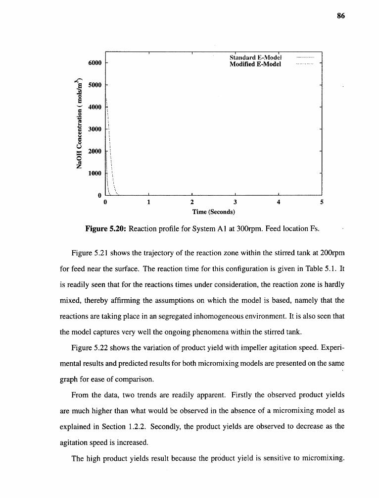
86

Figure 5.20: Reaction profile for System A 1 at 300rpm. Feed location Fs.

Figure 5.21 shows the trajectory of the reaction zone within the stirred tank at 200rpm

for feed near the surface. The reaction time for this configuration is given in Table 5.1. It

is readily seen that for the reactions times under consideration, the reaction zone is hardly

mixed, thereby affirming the assumptions on which the model is based, namely that the

reactions are taking place in an segregated inhomogeneous environment. It is also seen that

the model captures very well the ongoing phenomena within the stirred tank.

Figure 5.22 shows the variation of product yield with impeller agitation speed. Experi-

mental results and predicted results for both micromixing models are presented on the same

graph for ease of comparison.

From the data, two trends are readily apparent. Firstly the observed product yields

are much higher than what would be observed in the absence of a micromixing model as

explained in Section 1.2.2. Secondly, the product yields are observed to decrease as the

agitation speed is increased.

The high product yields result because the product yield is sensitive to micromixing.

Figure 5.21: Reaction zone trajectory. System Al, feed near liquid surface at 200rpm.

88

Fine scale fluid deformation (mesomixing and engulfment) are rate limiting and hence the

side reaction progresses to a greater extent than it would in a perfectly mixed system.

As the agitation speed is increased, the system approaches that of a perfectly mixed

system, and the role of micromixing diminishes. The observed product yields are still

relatively high in comparison to that of a perfectly mixed system.

The simulation predicts results in good agreement with the experimental data from the

literature. The simulation results from both micromixing models over predicts the final

selectivities somewhat, and this is a result of the fact that turbulence is over predicted for

this particular system.

Figure 5.22: Variation of product yield with agitation speed for System A 1. Feed locationFs.

5.3.6 Comparison of Predicted Product Yields for System A2 with Experiment

The results for System A2 are presented next. The trends observed for system Al are

observed for System A2 also. There are, however, differences that occur as a result of the

89

difference in viscosities.

In general, provided the flow remains turbulent, the change in viscosity has little influ-

ence on the bulk blending time (Bourne et al. 1995). Viscosity does, however, influence the

fine scale structure of the fluid. Since the fine scale structure controls the rate of micromix-

ing and hence controls the kinetics, it is expected that the viscosity will influence the yield

of the fast competitive reaction system used in this work. The engulfment parameter which

depends on the kinematic viscosity will be different for this system and hence different

results are to be expected.

The flow regime in stirred tank tanks is considered turbulent when the Reynolds number

exceeds a value of 1 x 10 4 . For Reynolds numbers in the range of 2000 to 1 x 10 4 , the flow

is considered to be transitional. Also, in the turbulent regime, the power number is constant

(Dickey and Fenic 1976) while lower in the transitional regime. The results presented in

Table 5.1 reflect this. The power number obtained for the viscous system are slightly lower

than those obtained for the aqueous system. However, it has been shown that even at the

lowest Reynolds numbers employed in this work, for this particular system, excellent fluid

turn over is obtained in the entire vessel (Bourne et al. 1995). Thus it seems certain that

fully developed turbulence is present for this system.

The reaction time history plots for this system exhibit the same trends as for System Al

(Figure 5.23 and Figure 5.24). The reaction times are, however, longer than for System A2

than for System Al under the same conditions. This is a result of the increase in viscosity.

An increase in viscosity slows the engulfment process i.e. the engulfment parameter is

decreased, as viscous forces are more prominent. Since engulfment strongly influences

the kinetics, the overall reaction time is longer. This is further evidence that micromixing

controls the kinetics.

Although the modified E-Model produces a different reaction profile than the standard

E-Model, the overall reaction times predicted by the two models do not differ significantly.

This indicates that, as the fluid viscosity is increased, the engulfment stage of micromixing,

90

the stage which results from the action of viscous forces, is more dominant.

Shown next is a plot showing the variation of product yield with impeller agitation

speed (Figure 5.25) The trends observed for System Al are observed here too. By-product

•formation decreases with increasing agitation speed.

Figure 5.23: Reaction time for System A2 at 100rpm. Feed location Fs.

5.3.7 Comparison of Predicted Product Yields for System A3 with Experiment

In this section results for System A3 are presented. System A3 is identical to system A 1 in

its configuration except that lower initial concentrations of reactants were used. This was

done in order to remain consistent with the results presented in later sections.

For the experimental phase of the work, the minimum feed time necessary for mi-

cromixing to be rate controlling was determined experimentally. The manner in which this

is done and the reasons why it was necessary are detailed in Section 4.3.

For this system, it was determined that a feed time of = 35 minutes (Figure 5.26) was

91

•Figure 5.24: Reaction time for System A2 at 300rpm. Feed location Fs.

sufficient to ensure that micromixing was dominant. This was the feed time used for all the

experimental runs.

As is evidenced here, except for the fact the the use of lower feed concentrations results

in faster reaction times and lower yields, all the trends observed in Section 5.3.2 are ob-

served here also. The reaction is faster at higher agitations speeds than at lower ones and

the inclusion of mesomixing parameter into the model results in the prediction of a slower

rate of reaction than when only the standard E-Model is considered.

The yield is observed to decrease with increasing agitation speed as expected and ob-

served earlier. The modified E-Model is observed to provide a better prediction of the

product yield than the standard E-Model. Both results are, however, most encouraging.

92

Figure 5.25: Variation of product yield with agitation speed for System A2. Feed locationFs.

5.3.8 Remarks

Mixing and chemical reaction were successfully simulated for the systems which consist

of a baffled cylindrical stirred tank fitted with a Rushton turbine at an impeller off bottom

clearance of one third the liquid height. System A2 differs from system A l in that a high

viscosity medium was used. System A3 differs from system Al in that lower initial reactant

concentrations were used.

The turbulence generated by this impeller was in general under-predicted. This led

an over-prediction of the reaction product yields. The prediction of turbulence was slightly

better for the viscous medium than for the aqueous medium. Nonetheless, the model serves

to provide insights into the micromixing process and the main trends of the process are also

captured. Reaction is slower at lower agitations speeds and the by-product yields higher,

indicating that the role of micromixing is more important when macromixing is slower.

The increase in fluid viscosity was observed to slow down the rate of micromixing and

Figure 5.26: Variation of product yield with feed time for System A3

Figure 5.27: Reaction profile for System A2 at 100rpm. Feed location Fs.

94

Figure 5.28: Reaction profile for System A3 at 300rpm. Feed location Fs.

hence increase the by-product yields. Thus in more viscous media, micromixing effects are

more important than in aqueous media.

The under-prediction of turbulence for the Rushton impeller could be attributed to mi-

cro instabilities (trailing vortices) present in the impeller region. These micro-instabilities

are an important source for the turbulence generated by this impeller. Because these insta-

bilities are transient in nature and occur at very small scales, it is very difficult to capture

them in a computational grid. This consequently leads to an under prediction of the turbu-

lence generated by the impeller. The Rushton turbine has been observed to generate two

such instabilities per blade (Zhou and Kresta 1996). The use of the MRF model which is

an steady state approximation of a transient process may fail to capture these phenomena in

sufficient detail. It is possible that only a fully time dependent computation in conjunction

with a turbulence model that can capture these phenomena will improve the prediction of

turbulence. A grid sufficiently small to capture their presence would not be feasible.

Despite its limitation, the CFD model has served to provide insights into the turbulent

Figure 5.29: Variation of Product Yield with Agitation Speed for System A3. Feed Loca-tion Fs.

mixing process.

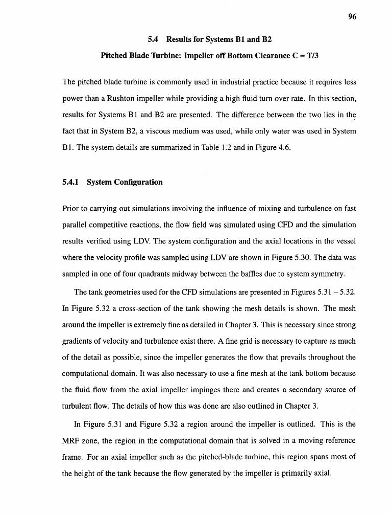
96

5.4 Results for Systems B1 and B2

Pitched Blade Turbine: Impeller off Bottom Clearance C = T/3

The pitched blade turbine is commonly used in industrial practice because it requires less

power than a Rushton impeller while providing a high fluid turn over rate. In this section,

results for Systems B1 and B2 are presented. The difference between the two lies in the

fact that in System B2, a viscous medium was used, while only water was used in System

B 1. The system details are summarized in Table 1.2 and in Figure 4.6.





where the velocity profile was sampled using LDV are shown in Figure 5.30. The data was

sampled in one of four quadrants midway between the baffles due to system symmetry.

The tank geometries used for the CFD simulations are presented in Figures 5.31 — 5.32.

In Figure 5.32 a cross-section of the tank showing the mesh details is shown. The mesh

around the impeller is extremely fine as detailed in Chapter 3. This is necessary since strong

gradients of velocity and turbulence exist there. A fine grid is necessary to capture as much

of the detail as possible, since the impeller generates the flow that prevails throughout the

computational domain. It was also necessary to use a fine mesh at the tank bottom because

the fluid flow from the axial impeller impinges there and creates a secondary source of

turbulent flow. The details of how this was done are also outlined in Chapter 3.

In Figure 5.31 and Figure 5.32 a region around the impeller is outlined. This is the

MRF zone, the region in the computational domain that is solved in a moving reference

frame. For an axial impeller such as the pitched-blade turbine, this region spans most of

the height of the tank because the flow generated by the impeller is primarily axial.

Figure 5.30: Stirred tank equipped with a pitched blade turbine at an impeller clearance of T/3: Locations where LDV data was taken.

98

Figure 5.31: Stirred tank equipped with a pitched blade turbine at an impeller clearance ofT/3: Outline grid.

Figure 5.32: Stirred tank equipped with a pitched blade turbine at an impeller clearance ofT/3: Outline grid showing mesh details.

99

Figure 5.33 shows a snapshot of the velocity profile for a simulation carried out at 300

rpm. The velocity vectors shown are the resultant velocity vectors for the axial, radial and

tangential directions. The velocity profile shown is typical of what one would expect from

an axial flow impeller. A turbulent jet is generated from the impeller and impinges on the

tank base. Two main circulation loops are evident. One on each side of the impeller. Thus

from a qualitative perspective, the simulation captures the main features of the turbulent

flow generated by the pitched-blade impeller.

5.4.2 Comparison of LDV Data with CFD Simulations for System B1

LDV data was taken on a system with an impeller agitation speed of 300rpm. The CFD

data presented here is for simulations carried out at 300rpm.

The pitched blade impeller produces two main circulation loops as shown in Fig-

ure 5.33. Near the tank wall along the entire length of the vessel axial velocities are positive

as the fluid is moving up. Near the shaft and above and below the impeller, the axial

velocities are negative as the fluid returns to the impeller and is pumped away towards the

tank base. These trends are reflected by the data, in particular in the region just above the

impeller. Near the top of the tank, the flow is more horizontal and "quiet". This trend has

been observed by other investigators of similar systems (Ranade and Joshi 1989b; Ranade

and Joshi 1989a).

Below the impeller, near the middle of the tank, positive velocities are observed indi-

cating the presence of a small recirculation loop there. This feature has also been reported

in the literature (Ranade and Joshi 1989b; Ranade and Joshi 1989a) and is characteristic of

similarly configured agitation systems.

Because the flow produced by the pitched-blade turbine is primarily axial in nature,

the radial components of the velocity are expected to be low. This is evidenced by the

simulation and verified by experiment as Figure 5.35 shows.

In the vicinity of the impeller region, the radial velocities are higher indicating that

Figure 5.33: Stirred tank equipped with a pitched blade turbine at an impeller clearance of T/3: Velocity profile.

Figure 5.34: Stirred tank equipped with a pitched blade turbine at an impeller clearance ofT/3: Comparison of experimental axial velocity data with CFD simulation.

102

the impeller imparts a some radial motion to the flow. In the rest of the vessel, the radial

velocity profiles are flat.

Figure 5.35: Stirred tank equipped with a pitched blade turbine at an impeller clearance ofT/3: Comparison of experimental radial velocity data with CFD simulation.

In the case of the tangential velocity (Figure 5.36), the results show that near the im-

peller shaft and along the height of the tank, swirling motion is evident. This swirling

motion dies out near the tank walls. The agreement between the predicted values and the

experimentally obtained ones is satisfactory.

Near the top of the vessel the profiles of turbulent kinetic energy are flat. Closer to the

103

Figure 5.36: Stirred tank equipped with a pitched blade turbine at an impeller clearance ofT/3: Comparison of experimental tangential velocity data with CFD simulation.

104

impeller, higher values are observed. The agreement between the experimental values and

the predicted values is satisfactory.

Figure 5.37: Stirred Tank Equipped with a Pitched Blade Turbine at an Impeller Clearanceof T/3: Comparison of Experimental Turbulent Kinetic Energy Data with CFD Simulation..

The CFD model captures the main features of the turbulent velocity field generated by

the pitched-blade impeller. Numerical discrepancies exist, but the results are satisfactory

overall.

105

5.4.3 Comparison of LDV Data with CFD Simulations for System B2

In this section, the results of performing the simulation in a viscous medium are presented.

The viscosity of the medium was 8.3 x 10 -3Pa • s and the manner whereby this was done

is presented in Chapter 4.

Figure 5.38: Stirred tank equipped with a pitched blade turbine at an impeller clearanceof T/3: Comparison of experimental axial velocity data with CFD simulation in viscousmedium.

106

Figure 5.39: Stirred tank equipped with a pitched blade turbine at an impeller clearanceof T/3: Comparison of experimental radial velocity data with CFD simulation in viscousmedium.

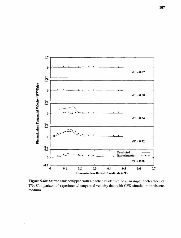
107

Figure 5.40: Stirred tank equipped with a pitched blade turbine at an impeller clearance ofT/3: Comparison of experimental tangential velocity data with CFD simulation in viscousmedium.

108

Figure 5.41: Stirred tank equipped with a pitched blade turbine at an impeller clearanceof T/3: Comparison of experimental turbulent kinetic energy data with CFD simulation inviscous medium.

109

5.4.4 Remarks

The same trends observed for the aqueous medium are observed for the viscous medium as

well. The CFD model is able to furnish without experimental input, a quantitative descrip-

tion of the turbulent flow field.


Table 5.2 shows how the computed power consumption of the system compares with ex-

perimentally measured power, as well as that computed using published correlations. It

is evident that the experimentally obtained values are in good agreement with those ob-

tained from published correlations. The computed power using CFD is also close to the

experimentally observed values, as well as the published correlations.

5.4.6 Comparison of Predicted Product Yields in Aqueous Medium with the Model


tion 4.3 are compared with the experimentally obtained results. The feed locations sim-

ulated are locations Fs and Fs2 (near the liquid surface) and Fi (in the impeller suction

stream) as outlined in Figure 4.7. Results obtained using both the standard E-Model as

well as the modified E-Model are presented on each plot.

Before proceeding with the experimental phase of the study, it was necessary to ex-

perimentally determine the minimum feed time necessary for micromixing to be rate con-

trolling as explained in Section 4.3. The results of this study are presented in Figure 5.42.

After ti 50-60 minutes, the product yield was observed to be independent of the feed rate,

thus the feed time employed for all subsequent simulations was taken to be 60 minutes.

In the following series of graphs (Figures 5.43 — 5.46) the concentration profile of

the limiting reagent, sodium hydroxide, is shown as a function of time. The graphs are

presented for a feed location near the liquid surface (Fs) and for one in the vicinity of the

Table 5.2: Power and mixing time characteristics for Systems B1 and B2

Figure 5.42: Variation of Product Yield with Feed Time for System B 1. Feed Location Fs..

impeller (Fi), and for both micromixing models at the lowest agitation speed (100 rpm),

and at the highest agitation speed used for this system (400 rpm).

Once again, it is evident that the two versions of the E-Model yield different time his-

tories for the limiting reagent. The two-parameter E-Model consistently predicts a slower

initial time history profile the the standard E-Model. As discussed earlier, this can be ex-

plained from the fact that the two-parameter E-Model includes information about the initial

breakup of the reaction zone prior to engulfment (mesomixing).

These reaction times are much smaller than the time taken to homogenize the tank con-

tents. A comparison of the mixing times with the reaction times is presented in Table 5.2.


as expected.

Figure 5.43: Reaction time for system B1 at 100rpm. Feed location Fs.

Figure 5.44: Reaction time for system B1 at 100rpm. Feed location Fi.


113


114

A comparison of the reaction zone trajectories shown in Figures 5.47 and 5.48, show

that for the short reaction times under consideration, the reaction zone mostly retains its

integrity. This means that the manner in which the model is used to account for the effects

of mixing on the kinetics is adequate — the reactions are taking place in a segregated zone

that is only a small part of the entire reactor volume.

The next series of plots (Figure 5.49 – Figure 5.51) show how the model performs at

predicting the final product yields for the reaction system.

In all cases, the trends observed for System A 1 and System A2, are observed here. The

by-product yield decreases with increasing agitation rate. When the feed is introduced in

the vicinity of the impeller, less by-product is formed than when the feed is introduced near

the liquid surface. The role of turbulence is thus important in determining the outcome of

the reactions.

Feed locations Fs (Figure 5.49) and Fs2 (Figure 5.50) yield similar results indicating

that near the liquid surface, the level of turbulence is similar irrespective of the radial po-

sition. In both cases, the by-product yields are over predicted. A reflection of the fact that

the turbulence was under predicted in the CFD simulation. The results are however most

encouraging. In particular, it is evident that the modified E-Model does a better job of

predicting the final product yield that the standard E-Model.

For feed location Fi (Figure 5.51, the model largely under predicts the final product

yields, and the two micromixing models yield similar results. The results are nonetheless

very encouraging.

5.4.7 Comparison of Predicted Product Yields in Viscous Medium with the Model

The results for System B2 are presented next. Experiments and simulations were carried

out for feed location Fs. The trends observed for System B1 are observed for System B2

also. There are, however, differences that occur as a result of the difference in viscosities.

It was first necessary to determine the minimum feed time necessary to ensure that

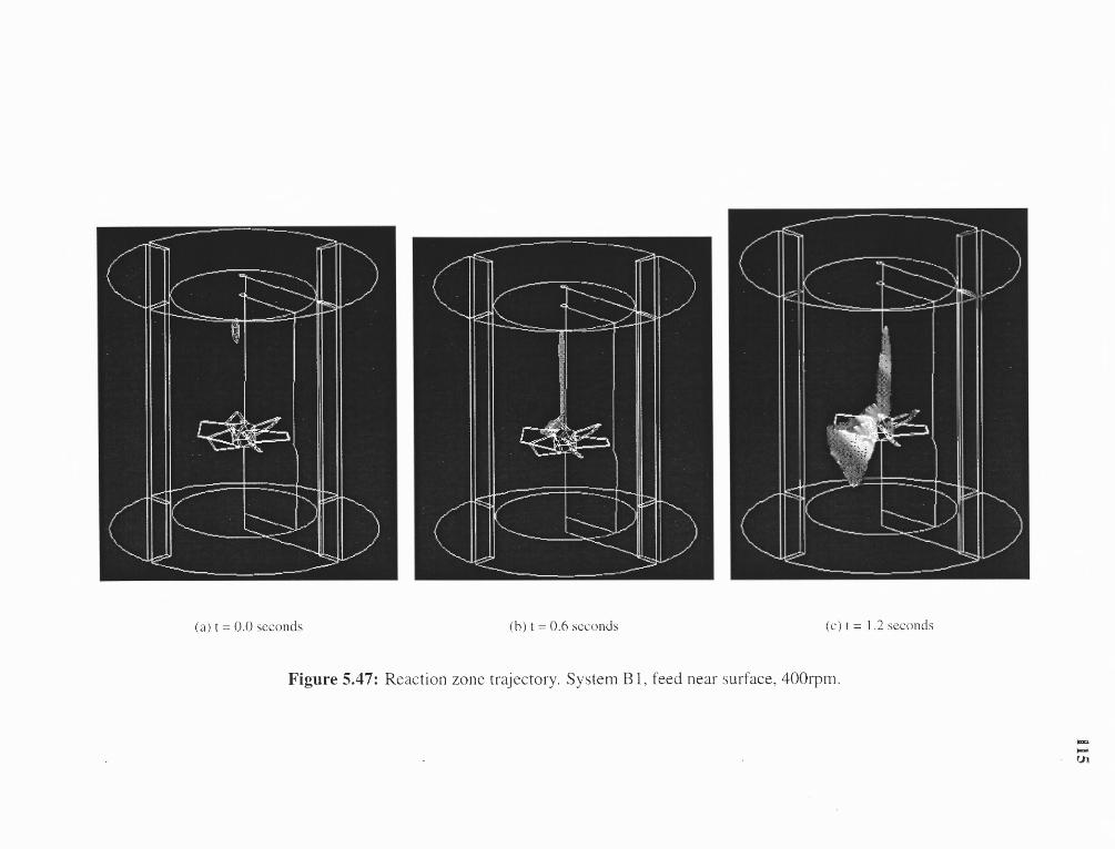
Figure 5.47: Reaction zone trajectory. System B 1, feed near surface, 400rpm.

Figure 5.48: Reaction zone trajectory. System B 1, feed above impeller, 400rpm.

Figure 5.49: Variation of Product Yield with Agitation Speed for System B 1. Feed Loca-tion Fs.

micromixing was the dominant mode of mixing. The results are presented in Figure 5.52.

From these result a feed time of 60 minutes was used in all the experimental runs.

The data presented in Table 5.2 show that the power number for this system is largely

constant and similar to that obtained for System B 1. Using this fact and the arguments

made earlier for System A2, we can assume that the flow for this system is turbulent.

The reaction time history plots (Figures 5.53 — 5.56) for this system exhibit the same

trends as for System Al, A2 and Bl. The complete set of results are presented in Table 5.2.

The reaction times are longer for system B2 than for System B 1. This results from the

increase in viscosity which slows down the engulfment process, i.e. the engulfment param-

eter is decreased. Since engulfment strongly influences the kinetics, the overall reaction

time is longer.

Figure 5.50: Variation of Product Yield with Agitation Speed for System B 1. Feed Loca-tion Fs2.

Figure 5.51: Variation of Product Yield with Agitation Speed for System B 1. Feed Loca-

tion Fi.

Figure 5.52: Variation of Product Yield with Feed Time for System B2



120


122

Shown next are plots showing the variation of the by-product yield with impeller ag-

itation speed (Figures 5.57 — 5.58). The by-product yield was observed to decrease with

increasing agitation speed. The model reasonably predicts the final product distributions.

Both version of the E-Model yield very similar results. This could be explained by the

fact that in the more viscous medium, the engulfment process is slower, and hence rate de-

termining for the micromixing process. Thus mesomixing, even if it were present, would

occur on a time scale much faster than mixing by engulfment and consequently would not

influence the final product distribution significantly.

Figure 5.57: Variation of Product Yield with Agitation Speed for System B2. Feed Loca-tion Fs.

Increasing the fluid viscosity has the effect of increasing the yield of by-product. This

result is consistent with established theory. Increasing the fluid viscosity results in a de-

crease in the rate of engulfment at the molecular level. This means that at microscopic scale

local inhomogeneities persist for a longer time thereby permitting the slower side reaction

to take place for a longer time before new material from the surrounding bulk is introduced.

123

Figure 5.58: Variation of Product Yield with Agitation Speed for System B2. Feed Loca-tion Fs.

The result is a higher rate of by-product formation.

5.4.8 Comparison of System B1 and System B2

The product yields observed for System B2 (viscous medium) were observed to be higher

that for System B1 (aqueous medium) when the same conditions and feed point were con-

sidered. In Figure 5.59, the results for feed location Fs (near the liquid surface) are super-

imposed for ease of comparison.

5.4.9 Remarks

The model was successfully used to predict the effect of mixing on the by-product yield for

the reaction system under study. It is evident that increasing the fluid viscosity significantly

impacts the kinetics and hence the formation of by-products.

Figure 5.59: Comparison of System B1 and System B2: Feed location Fs.

124

125

5.5 Results for System C

Chemineer High Efficiency Impeller (HE-3): Impeller off Bottom Clearance C = T/3

The Chemineer High Efficiency impeller (HE-3) is a hydrofoil impeller. Hydrofoil im-

pellers are popular for low viscosity applications because of their low power requirements

and high pumping capacities. In this section, results are presented for a system fitted with

a Chemineer HE-3 impeller. The system is configured as described in Table 1.2 and in

Figure 4.6.



parallel competitive reactions, the flow field was simulated using CFD, and the simulation


where the velocity profile was sampled using LDV are shown in Figure 5.60. Data was

sampled in each of four quadrants and averaged. This was done because the combination

of the three impeller blades and the four baffles on the tank results in a system that is non

symmetrical, thus there was no repeating cyclic geometry to exploit.

The tank geometry used for the CFD simulations are presented in Figures 5.61 — 5.62.

In Figure 5.62 a cross-section of the tank showing the mesh details is shown. A fine grid as

described in Chapter 3 was used as this was necessary to capture as much of the flow detail

as possible.

In Figure 5.61 and Figure 5.62 a region around the impeller is outlined. This is the

MRF zone. The region in the computational domain that is solved in a moving reference

frame. For a axial impeller such as the HE-3, this region does spans most of the height of

the tank because the flow generated by the impeller is primarily axial.

Figure 5.63 shows a snapshot of the velocity profile for a simulation carried out at

300 rpm. The velocity vectors shown are the resultant velocity vectors for the axial, radial

Figure 5.60: Stirred tank equipped with a Chemineer High Efficiency impeller at a clearance of T/3: Locations where LDV data wastaken.

127

Figure 5.61: Stirred Tank Equipped with a Chemineer High Efficiency Impeller at an im-peller clearance of T/3: Outline grid.

Figure 5.62: Stirred tank equipped with a Chemineer High Efficiency impeller at an im-peller clearance of T/3: Outline grid showing mesh details.

128

and tangential directions. The velocity profile shown is typical of what one would expect

from an axial flow impeller. A turbulent jet is generated from the impeller and impinges

on the tank base. Two main circulation loops are evident. One on each side of the im-

peller. Thus from a qualitative perspective, the simulation captures the main features of the

turbulent flow generated by the HE-3.

5.5.2 Comparison of LDV Data with FLUENT CFD Simulations

The LDV data was taken on a system with an impeller agitation speed of 330rpm and

compared with data from the numerical simulation.

The HE-3, like the PBT, produces two main circulation loops as shown in Figure 5.63.

Near the tank wall along the entire length of the vessel axial velocities are positive as the

fluid is moving up. Near the shaft and above and below the impeller, the axial velocities

are negative as the fluid returns to the impeller and is pumped away towards the tank base.

These trends are reflected by the data. Near the top of the tank, the flow is more hori-

zontal and "quiet". This trend has been observed by other investigators of similar systems

(Jaworski et al. 1996).

Because the flow produced by the HE-3 is primarily axial in nature, the radial com-

ponents of the velocity are expected to be low. This is evidenced by the simulation and

verified by experiment as Figure 5.65 shows.

The results show that near the impeller shaft and along the height of the tank, swirling

motion is evident. This swirling motion dies out near the tank walls. The tangential com-

ponent is still small in magnitude in comparison to the axial component of the velocity.

The agreement between the predicted values and the experimentally derived ones is good.

Near the top of the vessel the profiles of turbulent kinetic energy are flat. Closer to the

impeller, higher values are observed. The agreement between the experimental values and

the predicted values is satisfactory.

Figure 5.63: Stirred Tank Equipped with a Chemineer High Efficiency Impeller at an impeller clearance of T/3: Velocity profile.

Figure 5.64: Stirred Tank equipped with a Chemineer High Efficiency impeller at an im-peller clearance of T/3: Comparison of experimental axial velocity data with CFD simula-tion.

131

Figure 5.65: Stirred tank equipped with a Chemineer High Efficiency impeller at an im-peller clearance of T/3: Comparison of experimental radial velocity data with CFD simu-lation.

132

Figure 5.66: Stirred tank equipped with a Chemineer High Efficiency impeller at an im-peller clearance of T/3: Comparison of experimental tangential velocity data with CFDsimulation.

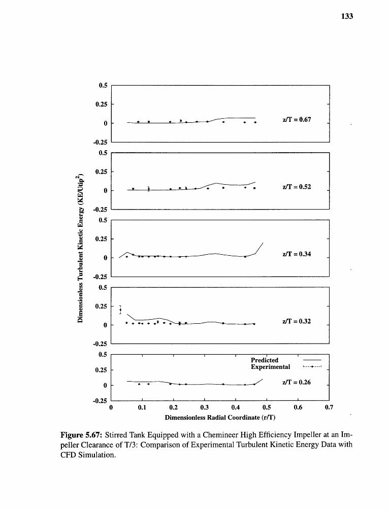
133

Figure 5.67: Stirred Tank Equipped with a Chemineer High Efficiency Impeller at an Im-peller Clearance of T/3: Comparison of Experimental Turbulent Kinetic Energy Data withCFD Simulation.

134


Table 5.5.3 shows how the computed power consumption of the system compares with

experimentally measured power values presented in the literature. It is evident that the

experimentally obtained values are in close agreement with those obtained from published

correlations. The computed power using CFD is also close to the experimentally observed

values, as well as the published correlations. In Table 5.5.3, some of the experimental data

are annotated with an asterisk. These are data points that could not be accurately sampled

because the signal produced by the strain gauges was extremely low for the system used.

These data points should thus be regarded with the understanding that they may not be

altogether accurate.

5.5.4 Remarks

The CFD model captures the main features of the turbulent velocity field generated by the

HE-3. Numerical discrepancies exist, but the results are overall satisfactory.

5.5.5 Comparison of Predicted Product Yields with the Model

In this section results are presented to show how well the model is able to predict the final

by-product distribution for System C.

The first step in the experimental investigation of the influence of mixing on the reaction

kinetics, was the determination of the minimum feed time to ensure that micromixing was

rate controlling. The results of this study are presented in Figure 5.68. From the results,

it was determined that a feed time of at least 90 minutes was necessary to ensure that the

reactions were conducted in a micromixing controlled regime. Thus a feed time of 90

minutes was used for all the experimental runs.

In the following series of graphs (Figures 5.69 — 5.72) the concentration profile of

the limiting reagent, sodium hydroxide, is shown as a function of time. The graphs are

Table 5.3: Power and mixing time results for System C

Figure 5.68: Variation of Product Yield with Feed Time for the HE-3

presented for a feed location near the liquid surface (Fs) and for one in the vicinity of the

impeller (Fi), and for both micromixing models at the lowest agitation speed (100 rpm),

and at the highest agitation speed used for this system (400 rpm). The complete set of

results are presented in Table 5.5.3.

It is evident that the two versions of the E-Model yield different time histories for the

limiting reagent. The two-parameter E-Model consistently predicts a longer time history

profile the the standard E-Model. As discussed earlier, this can be explained from the

fact that the two-parameter E-Model includes information about the initial breakup of the

reaction zone prior to engulfment (mesomixing).

The incorporation of mesomixing into the model results in a longer overall reaction

time. These reaction times are however much smaller than the time taken to homogenize

the tank contents. A comparison of the mixing times with the reaction times is presented

in Table 5.5.3.

The reaction times are observed to be faster at higher agitation speeds than at lower ones

as expected. In comparison to System B 1, the time taken to deplete the limiting reagent is

Figure 5.69: Reaction profile for system C at 100rpm. Feed location Fs.

137

Figure 5.70: Reaction profile for system C at 100rpm. Feed location Fi.

Figure 5.71: Reaction time for system C at 400rpm. Feed location Fs.

138

Figure 5.72: Reaction time for system C at 400rpm. Feed location Fi.

139

The next series of plots (Figure 5.73 and Figure 5.74) show how well the model per-

forms at predicting the final product yields for the reaction system.

In both cases, the trends observed earlier, are observed here. The by-product yield

decreases with increasing agitation rate. When the feed is introduced in the vicinity of the

impeller less by-product is formed than when the feed is introduced near the liquid surface.

It is evident here that the modified E-Model does a better job of predicting the final

product yield that the standard E-Model, in particular for the feed point Fs.

Figure 5.73: Variation of by-product yield with agitation speed for the HE-3. Feed locationFs

5.5.6 Remarks

The model was successfully used to predict the effect of mixing on the by-product yield for

the reaction system under study.

Figure 5.74: Variation of by-product yield with agitation speed for the HE-3. Feed locationFi.

141

5.6 Results for System D

Rushton Turbine: Impeller off Bottom Clearance C = T/2

Systems D consists of a baffled cylindrical vessel fitted with a Rushton turbine, such as

Systems A 1, A2. The difference between System D and the others lies in the fact that in

system D, the impeller was placed at an impeller off bottom clearance of T/2 rather than

T/3. The system details are summarized in Table 1.2 and in Figure 4.6.





where the velocity profile was sampled using LDV are shown in Figure 5.75.

The tank geometry used for the CFD simulations are presented in Figures 5.76 — 5.77.

In Figure 5.77 a cross-section of the tank showing the mesh details is shown. The mesh

around the impeller is extremely fine so as to capture as much of the flow detail as possible.

It was also necessary to use a fine mesh at the tank wall because the fluid flow from the

radial impeller impinges at the tank wall and creates a secondary source of turbulent flow

there. The manner whereby this was done is outlined in Chapter 3.

5.6.2 Comparison of LDV Data with FLUENT CFD Simulations

LDV data was taken on a system with an impeller agitation speed of 300rpm. The CFD

data presented here is for simulations carried out at 300rpm. As shown earlier, the Rushton

impeller produces four main circulation loops as shown in Figure 5.78. The axial velocity

results are presented in Figure 5.79. For this particular configuration, the loops are equal

due to the system symmetry. Near the tank wall and above the impeller the axial velocities

are positive as the fluid is moving up. Near the shaft and above the impeller, the axial

Figure 5.75: Stiffed tank equipped with a Rushton turbine at an impeller clearance of T/2: Locations where LDV data was taken.

143

Figure 5.76: Stirred tank equipped with a Rushton turbine at an impeller clearance of T/2:Outline grid.

Figure 5.77: Stirred Tank equipped with a Rushton turbine at an impeller clearance of 172 .:Outline grid showing mesh details.

Figure 5.78: Stirred tank equipped with a Rushton turbine at an impeller clearance of T/2: Velocity profile.

145

velocities are negative as the fluid returns to the impeller. These trends are reflected by the

data, in particular in the region just above the impeller. Below the impeller, the trend is

reversed, but the main features of flow are the same.

Figure 5.79: Stirred tank equipped with a Rushton turbine at an impeller clearance of T/2:Comparison of experimental axial velocity data with CFD simulation.

The radial velocity results are presented in Figure 5.80. In the upper portion of the

vessel, the radial velocities are negative, indicating a return of fluid from the tank walls to

the center of the tank as is shown in Figure 5.78.

The tangential velocity results are presented in Figure 5.81. The tangential velocities

are high in the vicinity of the impeller stream due to the rotation of the impeller while in

the general bulk, these velocities are small.

In regions far from the impeller, the predicted profiles of the turbulent kinetic energy

are generally good. The overall results are quite good.

146

Figure 5.80: Stirred tank equipped with a Rushton turbine at an impeller Clearance of T/2:Comparison of experimental radial velocity data with CFD simulation.

147

Figure 5.81: Stirred tank equipped with a Rushton turbine at an impeller clearance of T/2:Comparison of experimental tangential velocity data with CFD simulation.

148

Figure 5.82: Stirred tank equipped with a Rushton turbine at an impeller clearance of T/2:Comparison of experimental turbulent kinetic energy data with CFD simulation.

149

5.6.3 Remarks

The CFD model captures the main features of the turbulent velocity field generated by the

Rushton impeller. While numerical discrepancies exist, the overall agreement between the

LDV data and the CFD model is good.


Table 5.4 shows how the computed power consumption of the system compares with exper-

imentally measure power and published correlations. It is evident that the experimentally

obtained values are in close agreement with those obtained from published correlations

while the computed power is under-predicted.

5.6.5 Comparison of Predicted Product Yields with the Model


tion 4.3 are compared with the experimentally obtained results from our laboratory. The

feed locations simulated are locations Fs (near the liquid surface), location Fi (in the im-

peller suction stream), and location Fd (the impeller discharge stream) as outlined in Fig-

ure 4.7. Results obtained using both the standard E-Model as well as the modified E-Model

are presented on each graph.

As with all systems investigated, it was necessary to determine the minimum feed time

required to establish a system where micromixing was rate controlling. The results of the

study are presented in Figure 5.83. It is seen that a feed time of 20 minutes is sufficient to

ensure that micromixing is rate controlling.

The following series of plots (Figures 5.84— 5.87) show the concentration profile of the

limiting reagent, sodium hydroxide, as a function of time. The graphs are presented for

feed locations Fs and Fi, and for both micromixing models at the lowest agitation speed

(100 rpm), and at the highest agitation speed used for this system (300 rpm). The complete

Table 5.4: Power and mixing time characteristics for System D

Figure 5.83: Variation of product yield with feed time for System D

set of data is presented in Table 5.4.

Again, it is evident that the two versions of the E-Model yield different time histories

for the limiting reagent. The overall reaction time predicted by both models are similar and

much smaller than the mixing time for this vessel.


indicating that the role of micromixing diminishes with increasing agitation speed. This is

consistent with the trends observed for the other systems studied.

The predicted selectivities follow the previously observed trends: by-product formation

decreases with increasing agitation rate and feeding material in the vicinity of the impeller

results in lower by-product yields also.

The amount of by-product formation for all three locations are similar. With less by-

product being formed in the impeller discharge stream than at the other two points in the

system, indicating the higher level of turbulence that prevails there.

Figure 5.84: Reaction profile for System D at 100rpm. Feed location Fs.

152

Figure 5.85: Reaction profile for System D at 100rpm. Feed location Fi.

153

Figure 5.86: Reaction profile for System D at 300rpm. Feed location Fs.

5.6.6 Effect of Impeller Off-bottom Clearance

As mentioned earlier, raising the the impeller off-bottom clearance for the Rushton-based

systems had the effect of lowering the amount of undesired by-product that was formed.

Results for System A3 are presented with results for System D, for feed location Fs, in

Figure 5.91 for ease of comparison.

The difference between the predicted data is greater than the difference between the ex-

perimental data. Nonetheless, it is evident that increasing the impeller off-bottom clearance

impacts the yield of the undesired by-product.

154

Figure 5.87: Variation of product yield with feed time for System D at 300rpm. Feedlocation Fi.

Figure 5.88: Variation of product yield with agitation speed for System D. Feed Location

Fs.

155

Figure 5.89: Variation of product yield with agitation speed for System D. Feed locationFi.

Figure 5.90: Variation of product yield with agitation speed for System D. Feed location

Fd.

156

Figure 5.91: Effect of increasing the impeller off-bottom clearance: Comparing SystemA3 and System D

CHAPTER 6

CONCLUSION

In this work two state of the art technologies, Laser Doppler Velocimetry (LDV) and Com-

putational Fluid Dynamics (CFD), were used to investigate the effect of turbulent mixing

fast parallel competing reactions in baffled stirred tanks. A commercially available CFD

package (FLUENT) was used to predict the three dimensional velocity profile and profiles

of turbulent kinetic energy and local energy dissipation rates, as well as power consumption

within the mechanically agitated vessels. The Reynolds Stress Model (RSM) was used to

account for turbulence effects in the flow field and the Multiple Reference Frames (MRF)

model was used to simulate the motion of the agitator. A novel model that combined CFD,

and micromixing models was developed and used to investigate the effect of mixing on

chemical reactions for a variety of systems.

There were two components to the experimental phase of this work. The first compo-

nent involved carrying out the reaction scheme in the mixing laboratory in the department

of Chemical Engineering, Chemistry and Environmental Science at the New Jersey Insti-

tute of Technology, under a variety of conditions. This involved varying the following

parameters:

• The agitator: Three different impellers were used used in this study. These were

namely the Rushton turbine, the 6 Bladed Pitched Blade turbine (6 PBT) and the

Chemineer High Efficiency impeller (HE-3). The three impellers cover the range of

mixers used in industrial practice for low viscosity blending applications.

• The agitation speed: For each impeller studied, the agitation rate was varied in order

to determine its effect on the yield of the reactions.

• The feed point location: The location in the vessel where the feed was introduced

was varied to study what effects this would have on the yield.

• The fluid viscosity: The viscosity of the fluid was varied for two of the systems,

157

158

namely the Rushton equipped system and the 6 PBT equipped system.

• The impeller off bottom clearance: The impeller off bottom clearance was varied

for the Rushton equipped systems.

The experimental data served not only to validate the novel approach developed in this

work, but also to study how turbulent mixing for complex reactions systems is influenced

by the reactor setup. In so doing the general applicability and flexibility of the new model

were also established.

The second component of the experimental work involved the use of the LDV apparatus

to experimentally measure the three dimensional velocity profile of the flow field within the

agitated vessels along with the fluctuating components of these velocities. The fluctuating

components of the velocity were used to determine the turbulent kinetic energy of the flow

within the vessels. This experimental work served primarily to validate the predictions

furnished by the CFD model.

The micromixing effects were accounted for using Engulfment based models. The stan-

dard E-Model and a variant which accounted for mesomixing as well as micromixing by

engulfment were used. The reactant fed to the system was simulated using the Volume of

Fluid (VOF) multiphase model. The micromixing model, VOF model, and the informa-

tion furnished by CFD were then coupled in a novel way to yield a novel model that can be

used to predict the yield of reaction systems exhibiting complex chemistry in baffled stirred

tanks.

The main results for the baffled cylindrical vessel fitted with a Rushton turbine can be

summarized as follows:

• While the three dimensional velocity profile was well predicted, turbulence and

power were under predicted. This had the effect of over predicting the product yields.

• The model was able to successfully capture the effect of varying the agitation speed,

fluid viscosity and impeller off bottom clearance on the reaction system.

159

• Increasing the agitation speed of the impeller resulted in a decrease of the level of

by-product formation.

• Increasing the viscosity of the fluid had the effect of increasing amount of by-product

formation. The observed phenomena highlight the importance of micromixing in

determining the outcome of parallel competitive reactions in turbulent environments.

• When the impeller off bottom clearance was increased, a drop in by-product forma-

tion was observed for feed material introduced near the liquid surface indicating an

increase in the turbulence level for that region.

The main results for the baffled cylindrical vessel fitted with a 6 bladed pitched blade

turbine can be summarized as follows:

• The three dimensional velocity profile was well predicted, as well as the turbulence

and power.

• Again, the model was able to successfully capture the effect of varying the agitation

speed, fluid viscosity on the levels of by-product formation.


by-product formation as for the Rushton based systems.

• Increasing the viscosity of the fluid had the effect of increasing amount of by-product

formation.

The main results for the baffled cylindrical vessel fitted with a Chemineer High Effi-

ciency impeller can be summarized as follows:

• The three dimensional velocity profiles were well predicted, as well as the turbulent

kinetic energy and power delivered to the system by the impeller.

• Again, the model was able to successfully capture the effect of varying the agitation

speed on the levels of by-product formation.

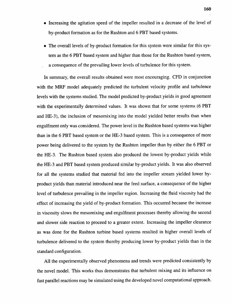
160


by-product formation as for the Rushton and 6 PBT based systems.

• The overall levels of by-product formation for this system were similar for this sys-

tem as the 6 PBT based system and higher than those for the Rushton based system,

a consequence of the prevailing lower levels of turbulence for this system.

In summary, the overall results obtained were most encouraging. CFD in conjunction

with the MRF model adequately predicted the turbulent velocity profile and turbulence

levels with the systems studied. The model predicted by-product yields in good agreement

with the experimentally determined values. It was shown that for some systems (6 PBT

and HE-3), the inclusion of mesomixing into the model yielded better results than when

engulfment only was considered. The power level in the Rushton based systems was higher

than in the 6 PBT based system or the HE-3 based system. This is a consequence of more

power being delivered to the system by the Rushton impeller than by either the 6 PBT or

the HE-3. The Rushton based system also produced the lowest by-product yields while

the HE-3 and PBT based system produced similar by-product yields. It was also observed

for all the systems studied that material fed into the impeller stream yielded lower by-

product yields than material introduced near the feed surface, a consequence of the higher

level of turbulence prevailing in the impeller region. Increasing the fluid viscosity had the

effect of increasing the yield of by-product formation. This occurred because the increase

in viscosity slows the mesomixing and engulfment processes thereby allowing the second

and slower side reaction to proceed to a greater extent. Increasing the impeller clearance

as was done for the Rushton turbine based systems resulted in higher overall levels of

turbulence delivered to the system thereby producing lower by-product yields than in the

standard configuration.

All the experimentally observed phenomena and trends were predicted consistently by

the novel model. This works thus demonstrates that turbulent mixing and its influence on

fast parallel reactions may be simulated using the developed novel computational approach.

161

The approach is completely general requiring no adjustable parameters and is therefore

applicable to a wide variety of systems.

APPENDIX A

FORTRAN CODE USED IN THE EVALUATION OF THE MICROMIXING

MODEL EQUATIONS

A.1 Runge-Kutta Solver

The Runge-Kutta code used in solving the model equations was obtained from an online

numerical library, Netlib. Pertinent information are as follows:

RKSUITE Release 1.0 November 1991written by

R.W. Brankin (*), I. Gladwell(**), and L.F. Shampine (**)

(*) Numerical Algorithms Group Ltd.

Wilkinson HouseJordan Hill RoadOxford OX2 8DRU.K.email: [email protected]

[email protected] phone: + 44 865 511245International fax: + 44 865 310139

(**) Department of MathematicsSouthern Methodist UniversityDallas, Texas 75275U.S.A.email: [email protected]. phone: (214) 692-2542U.S. fax: (214) 692-4138

RKSUITE is a suite of codes based on Runge-Kutta methods for the numericalsolution of the initial value problem for a first order system of ordinarydifferential equations. It is the result of decades of research anddevelopment of such methods and software by the authors. It supersedessome very widely used codes written by the authors and their coauthors,namely, the RKF45 code that is available in several books and its descendantDDERKF in the SLATEC library, and DO2PAF and the associated codes in the NAGFortran library.

162

163

RKSUITE is being made available free of charge to the scientificcommunity as a public service. It is expected that anyone making asubstantial use of the software will acknowledge this use and inparticular, give a proper citation in any publication resulting fromits use. A suitable reference is:

R.W. Brankin, I. Gladwell, and L.F. Shampine, RKSUITE: a suite ofRunge-Kutta codes for the initial value problem for ODEs, Softreport92-S1, Department of Mathematics, Southern Methodist University,Dallas, Texas, U.S.A, 1992.

A.2 Driver Module

The driver module was written to read in the initial conditions and system parameters, these

include initial concentrations and the amount of feed discretization. The driver module was

also responsible for performing the necessary mass balances and updating the boundary

conditions.

program emodel 'driver

implicit real (a-h,o-z)

c cc Simulation of micromixing in stirred tankc Choice of Model used is as follows:c cc 1. Original E-Model (R 14)c 2. Modified E-Model (R10)cc cc The W-Z Transformation was used so that it was possible to solve the cc problem with a Runge-Kutta Scheme and NOT collocationc this file emodel'driver' voff goes with emodel ' solve' vof.fc and rksuite.fc cc -Otute 25 Jan 1999c c

c c

c my variable declarationsc c

c---nsize denotes the max number of I slicesc---ncomp denotes the max number of species

integer ncomp,nrow,ncol,ntimesparameter(ncomp=7,nrow=500,ncol=3)

c real conc(1:ncomp),avgconc(1:ncomp)real edata(1:nrow,1:ncol)real avgdiss,avgkin

c status is used to determine whther the soln process isc running smoothly or not. if not, then the process is terminatedc and answers up to that point are printed out.

status = 0step = 1

c read in the file conating the epsilon and ke values from FLUENTopen(10,file='vof'fs.data')kount = 0write(*,*) 'Reading Data'do 93 krow = 1,nrow

read(10,1020,end=94) (edata(krow,kcol), kcol=1,ncol)write(*,1020) (edata(krow,kcol), kcol=1,ncol)

93 continue94 continue

c back one step from the EOF markerkount = kount - 1

c first time will be used as time zerotime0 = edata(1,1)

cc USER INPUTSc

c Model to be used:c 1 -i, Standard E Modelc 2 Modified E Model

nmodel = 1c parameters to sendc va,vb,average dissipation rate,concentrationsc Tank Bulk Volume

vb = 0.019e0vbl = vb

c Volume Added to the Tankvatot = vb/50.0e0

164

c number of parts feed is discretized into -i, sigmasigma = 50.0e0ntimes = NINT(sigma)

c volume of first partval = vatot/sigma

c initial concentrationsCAo = 900.0e0CBo = 0.00e0CCo = 0.00e0

c initial average concentrations - zone 1CAavg = 0.0d0CBavg = 18.0e0CCavg = 18.0e0

c put the above concentrations into arraysconc(1) = CAoconc(2) = CBoconc(3) = CCoavgconc(1) = CAavgavgconc(2) = CBavgavgconc(3) = CCavg

c loop sigma times until all the feed has been addedopen(12,file=' ca . profile • start.data')open(13,file.' ca . profile 'end.data')do 401 nfeed = 1,ntimes

nstep = 2nstepl = nstep - 1va = val

c...parameters wantedc...new concentrations, new va,new vbc loop until all the feed has been consumed503 continue

tstart = edata(nstep1,1)tend = edata(nstep,1)tstart = tstart - time°tend = tend - time°avgdiss = edata(nstep,2)avgkin = edata(nstep,3)print*,'nstep',nstepprint*,'tstare,tstartprint*,'tend',tend

call rkmixer(va,vb,avgdiss,avgkin,conc,avgconc,tstart,tend,nmodel)

print 1505print 3005,conc(1),conc(2),conc(3)

c update concentrations in entire tank

165

nstep = nstep + 1nstepl= nstep - 1if (nfeed .eq. 1) then

write (12,1030) tend,conc(1),conc(2),conc(3)elseif (nfeed .eq. ntimes) then

write (13,1030) tend,conc(1),conc(2),conc(3)endifif (conc(1) .gt. 0.0e0) goto 503

do 402 nspec = 1,3avgconc(nspec) = (avgconc(nspec)*vb+conc(nspec)*va)/(va+vb)

402 continuec Echo Results to Screen

print*,'vafinal ',vavb = vb + vava = 0.0e0conc(1) = CAoconc(2) = CBoconc(3) = CCo

401 continueprint*,'The final Concentrations in the Bulk Are: 'print 1500print 3000,avgconc(1),avgconc(2),avgconc(3)print*,'The Final Volumes Are'print*,'VA',vaprint*,'VB',vbprint*,' Computing the selectivity'xs = (CCavg*vb1-avgconc(3)*(vb))/(CAo*vatot)print*,'Xs',xsclose(10)close(12)close(13)

1500 Format(6x,6x,'CAavg',12x,'CBavg',12x,'CCavg')3000 Format(9x,lx,3(E14.6,3x))1505 Format(6x,6x,'CA',12x,'CB',12x,'CC')3005 Format(9x,lx,3(E14.6,3x))1020 format(lx,e15.6,2x,e15.6,2x,e15.6)1030 format(1 x,4(E 14.6,2x))

end

166

167

A.3 Solver Module

The solver module interfaced directly with the Runge-Kutta solver. It takes the necessary

parameters from the driver module passes them on to the Runge-Kutta code. The solutiorth

are then returned to the driver module for updating. It also contains the equations that need

to be solved.

subroutine rkmixer(avol,bvol,avgdiss,avgkin,conc,& avgconc,t1,t2,nmodel)

c cc This subroutine solves two verions of the emodel cc cc nmodel = 1 -i, Conventional E-Model R14 cc nmodel = 2 -i, Modified Emodel R10 cc c

•c The W-Z Transformation was used so that it was possible to solve the cc problem with a Runge-Kutta Scheme and NOT collocation cc this file emodel'solve'vof.f goes with emodel'driver'voff cc and rksuite.f cc cc -Otute 25 Jan 1999 cc c

C NOTES: Typically problems are solved for a number of tolerances, initialC conditions, intervals, parameter values, ... . A prudent personC would make at least one run with global error assessment as aC spot check on the reliability of the results. Variant lb showsC how to do this.CC For TOL in this range, METHOD = 2 is generally the most efficientC choice. Indeed, for this specific problem and tolerance (and aC specific computer, precision, compiler, ... ), the results foundC in tmpl 1 .out show that the cost with METHOD = 2 is 109 calls toC the subroutine F, with METHOD = 1 it is 292 calls, and withC METHOD = 3 it is 105 calls. At relaxed tolerances, METHOD = 1 isC generally the most efficient choice, and at stringent tolerances,C METHOD = 3 is generally the most efficient.CC In typical use of UT, the cost is scarcely affected by theC number of answers, but when a "large" number of answers isC required, this is not true of METHOD = 3. In such a situation

168

C its cost is proportional to the number of answers.CC Working storage must be provided in the array WORK(*) of lengthC LENWRK. Because storage is no problem with only NEQ = 2C equations, LENWRK is taken here to be 32*NEQ, enough to handleC all three methods with and without global error assessment.CC .. Parameters .. •c Make changes NEQ,METHOD

implicit double precision (a-h,o-z)

INTEGER NEQ, LENWRK, METHOD,ncompPARAMETER (NEQ=3,LENWRK=64*NEQ,METHOD=3,ncomp=7)

cC .. Local Scalars ..

DOUBLE PRECISION HNEXT, HSTART, T, TEND,& TLAST, TOL, TSTART, TWANT, WASTE

•INTEGER L, NOUT, STPCST, STPSOK, TOTF, UFLAGLOGICAL ERRASS, MESAGE

C .. Local Arrays ..DOUBLE PRECISION THRES(NEQ), WORK(LENWRK), Y(NEQ), YMAX(NEQ),& YP(NEQ), YSTART(NEQ)

c MY VARIABLES ARE DECLARED FROM HERE ON

c imported real variablesreal conc(1:ncomp),avgconc(1:ncomp),. time,avgdiss,avgkin

real avol,bvol,tl,t2

c parameters needed to solve the eqns. these will be declared inc a common block

double precision dengulf,corrsin,dkvall,dkval2double precision kviscdouble precision x,xb,kedouble precision CAo,CBo,CCodouble precision CAbar,CBbar,CCbar

c common /oparams/dengulf,corssin,dkvall,dkval2,vaocommon /oavgs/ uavg,CCbar

C .. External Subroutines ..EXTERNAL F 1,F2, SETUP, STAT, UT

C .. Executable Statements ..

c Make changes: TSTART,YSTART(NEQ),TLAST,TEND.

C C Set the initial conditions. Note that TEND is taken well pastC the last output point, TLAST. When this is possible, and itC usually is, it is good practice. .C

print*,'entering rkmixerl subroutine to solve eqns'

c volumeova = DBLE(avol)ovb = DBLE(bvol)vao = ovaovtot = ova + ovb

print*,'VA',avolprint*,'VB',bvol

c initial concentrations - micro mixed phaseCAo = DBLE(conc(1))CBo = DBLE(conc(2))CCo = DBLE(conc(3))

print*,'concentrations updated'

c initial average concentrations - bulk zoneCAbar = DBLE(avgconc(1))CBbar = DBLE(avgconc(2))CCbar = DBLE(avgconc(3))

print*,' average concentrations updated'c

print*,' Initial Concentrations Before Solving'print 1000print 2000,CAo,CBo,CCoprint*,'Average Concentrations Before Solving'print 1500print 3000,CAbar,CBbar,CCbar

169

c stopc

viscosity = 9.0d-4density = 1.0d3pi = 3.14159265359diss = DBLE(avgdiss)ke = DBLE(avgkin)kvisc = viscosity/density

c diffusivitydiff = ld-9

c lifetime of a vortexalpha = 12.0d0*(kvisc/diss)**0.5

c alpha = 1d-5x = alpha

c ENGULFMENT RATEc dengulf = 0.058d0*(diss/kvisc)**0.5

dengulf = DLOG(2.0d0)/alphadengulf2=dengulf

c CORSSIN TIME CONSTANTschmidt = viscosity/(density*diff)

c tms = 5.74*(ke/diss) +c . (1.0/2.0)*(kvisc/diss)**(1.0/2.0)*DLOG(schmidt)

tms = 0.5d0*(ke/diss)c A = 2.0d0c D = 0.1d0c rlambda = D/10.0d0c tms = A*(rlambda**2/diss)**(1.0d0/3.0d0)

corssin = 1/tmsc

xb=0dkvall = 1.0d5dkval2 = 0.020d0dtemp = 273.15d0 + 23.0d0dR = 8.314dkval2 = 2.0d5*dexp(-3.891d4/(dR*dtemp))print*,'Parameters are as follows:'print*,'viscosity: ',viscosityprint*,'density: ',densityprint*,'dissipation: ',dissprint*,'ke',keprint*,'schmidt',schmidtprint*,' kl: ',dkvallprint*,'k2: ',dkval2print*,'kinematic viscosity',kviscprint*,'Vortex Lifetime: ',alpha

170

print*,'E: ',dengulf2print*,'corssin',corssin

c transform the variables - micro mixed phaseuavg = CAbar - CBbaruo = CAo - CBoCCbar = CCbar * 1.0d0

c boundary conditionsc TSTART = 0

YSTART(1) = uoYSTART(2) = CCo

c and then the volumesYSTART(3) = ovaYSTART(4) = ovbTSTART = DBLE(t1)TEND = 2*DBLE(t2)TWANT = DBLE(t2)

C C Initialize output.Cc print out the initial conditions

print 9010print 9030,TSTARTprint 9040,TWANTprint 9070print 9020

C C C Set error control parameters.C

TOL = 5.0D-5DO 20 L = 1, NEQ

THRES(L) = 1.0D-1020 CONTINUE

CC Call the setup routine. Because messages are requested, MESAGE = .TRUE.,C there is no need later to test values of flags and print out explanations.C In this variant no error assessment is done, so ERRASS is set .FALSE..C By setting HSTART to zero, the code is told to find a starting (initial)C step size automatically .C

MESAGE = .TRUE.ERRASS = .FALSE.HSTART = ZERO

C

171

172

c results are obtained here. where twant is the point at which a soln .c is wanted

if (nmodel .eq. 1) thenprint*,'calling setup routine for R14'

CALL SETUP(NEQ,TSTART,YSTART,TEND,TOL,THRES,METHOD,'Usual Task'& ,ERRASS,HSTART,WORK,LENWRK,MESAGE)

print*,'calling ut routine for R14'CALL UT(F1,TWANT,T,Y,YP,YMAX,WORK,UFLAG)

else if (nmodel .eq. 2) thenprint*,'calling setup routine for R10'

CALL SETUP(NEQ,TSTART,YSTART,TEND,TOL,THRES,METHOD,'Usual Task'& ,ERRASS,HSTART,WORK,LENWRK,MESAGE)

print*,'calling ut routine for R10'CALL UT(F2,TWANT,T,Y,YP,YMAX,WORK,UFLAG)

endifC

IF (UFLAG.GT.2) GO TO 60C Success. T = TWANT. Output computed and true solution components.c print solutions after first transforming the variables back toc concentrations

u= Y(1)CC = Y(2)ova = Y(3)

c ovb = Y(4)ovb = ovtot - ovaCA = (DABS(u)+u)/2CB = (DABS(u)-u)/2

c print 1000print 2000,CA,CB,CC

avol = REAL(ova)bvol = REAL(ovb)

c update the concentrations

conc(1) = REAL(CA)conc(2) = REAL(CB)conc(3) = REAL(CC)

c stop

C The integration is complete or has failed in a way reported in aC message to the standard output channel.60 CONTINUE

CC YMAX(L) is the largest magnitude computed for the solution componentC Y(L) in the course of the integration from TSTART to the last T. ItC is used to decide whether THRES(L) is reasonable and to select a newC THRES(L) if it is not.C

print 9070print *

c WRITE (*,'(A/)') ' YMAX(L) 'c DO 80L = 1, NEQc WRITE (*,' (13X,1PE8.2)') YMAX(L)c 80 CONTINUECC The subroutine STAT is used to obtain some information about the progressC of the integration. TOTF is the total number of calls to F made so farC in the integration; it is a machine-independent measure of work. At presentC the integration is finished, so the value printed out refers to the overallC cost of the integration.C

print 9070

c stop

CALL STAT(TOTF,STPCST,WASTE,STPSOK,HNEXT)WRITE (*,' (/A,1PE10.2,0P/A,I10/A,I10/A,F10.2/A,I10)')& ' The integration reached TNOW,& ' The cost of the integration in calls to F was', TOTF,& ' The number of calls to F per step is ', STPCST,& ' The fraction of failed steps was ', WASTE,& ' The number of accepted steps was STPSOK

c print line to signal end of resultsprint 9070

c format statements for displaying results9010 format(lx,32(' ),' Results' ,31(' ))9020 format(lx,'Initial Conditions')9030 format(lx,'Start Time = ',f10.4)9040 format(lx,'End Time = ',f 10.4)

173

9050 format(lx, ' Results' )9060 format(lx,5x,'Y' ,I2, ' = ' ,f10.4)9070 format(1x,70('-' ))

1000 Format(lx,6x,'CA',15x,'CB',15x,'CC')1500 Format(6x,6x,'CAavg',12x,'CBavg',12x,'CCavg')1505 Format(6x,6x,'CAb',14x,'CBb',14x,'CCb')2000 Format(1x,1x,3(D14.6,3x))3000 Format(9x,1x,3(D14.6,3x))

RETURNEND

CSUBROUTINE F1(T,Y,YP)implicit double precision(a-h,o-z)

C .. Scalar Arguments ..DOUBLE PRECISION TDOUBLE PRECISION dengulf,corrsin,dkvall,dkval2,vaoDOUBLE PRECISION uavg,CCavg

C .. Array Arguments ..DOUBLE PRECISION y(*), YP(*)

C .. Executable Statements ..common /oparams/dengulf,corrsin,dkvall,dkval2,vaocommon /oavgs/ uavg,CCbar

c print*, 'corrsin',corrsinc print*,'dengulf',dengulfc print*,'dkval2',dkval2

corrsin = corrsin* 1.0d0dengulf = dengulf* 1.0d0dkval2 = dkval2 *1.0d0uavg = uavg* 1.0d0CCbar = CCbar* 1.0d0ca = ( DABS(Y(1))+Y(1) )/2.0cc = Y(2)YP(1) = (dengulf)*(uavg - Y(1)) - dkval2*ca*ccYP(2) = (dengulf)*(CCbar - Y(2)) - dkval2*ca*ccYP(3) = (dengulf)*Y(3)RETURNEND

CSUBROUTINE F2(T,Y,YP)implicit double precision(a-h,o-z)

C .. Scalar Arguments ..

174

DOUBLE PRECISION TDOUBLE PRECISION dengulf,corrsin,dkval 1,dkval2,vaoDOUBLE PRECISION uavg,CCavg

C .. Array Arguments ..DOUBLE PRECISION Y(*), YP(*)

C .. Executable Statements ..common /oparams/dengulf,corssin,dkvall,dkval2,vaocommon /oavgs/ uavg,CCavgfactor = (1 - (Y(3)*DEXP(- T*corssin)/vao))ca = ( DABS(Y(1))+Y(1) )/2cc = Y(2)YP(1) = dengulf*factor*(uavg - Y(1)) - dkval2*ca*ccYP(2) = dengulf*factor*(CCavg - Y(2)) - dkval2*ca*ccYP(3) = dengulf*factor*Y(3)RETURNEND

C

175

REFERENCES

Armenante, P. M. and C. Chou. "Experimental LDV Measurements and Numerical CFDDetermination of the Fluid Velocity Distribution in an Unbaffled Vessel." AICHESymposium Series 90 (1994): 33-40.

Armenante, P. M., C. Chou, and R. R. Hemrajani. "Comparison of Experimental andNumerical Fluid Velocity Distribution Profiles in an Unbaffled Mixing Vessel Pro-vided with a Pitched-Blade Turbine." Institution of Chemical Engineers SymposiumSeries 136. Cambridge, England: Institution of Chemical Engineers, September 1994,349-356.

Armenante, P. M., C. Luo, C. Chou, I. Fort, and Jaroslav Medek. "Velocity Profilesin a Closed, Unbaffled Vessel: Comparison Between Experimental LDV Data andNumerical CFD Predictions." Chemical Engineering Science 52 (1997): 3483-3492.

Aubry, C. and J. Villermaux. "Representation du Mélange Imparfait de Deux Courants deReactifs dans un Réacteur Agité Continu." Chemical Engineering Science 30 (1975):1309-1313.

Bakker, R. A. and H. E. A. van den Akker. "A Computational Study of Chemical Reactorson the Basis of Micromixing Models." Transactions of the Institution of ChemicalEngineers 72 (November 1994): 733.

Bakker, R. A. and H. E. A. van den Akker. "A Lagrangian Description of Micromixing in aStirred Tank Reactor Using 1D-micromixing Models in a CFD Flow Field." ChemicalEngineering Science 51 (1996): 2643-2648.

Baldyga, J. "Turbulent Mixer Model with Application to Homogeneous, InstantaneousChemical Reactions." Chemical Engineering Science 44 (1989): 1175-1182.

Baldyga, J. "A Closure Model for Homogeneous Chemical Reactions." Chemical Engi-neering Science 49 (1994): 1985-2003.

Baldyga, J. and J. R. Bourne. "A Fluid Mechanical Approach to Turbulent Mixing andChemical Reaction - Part II: Micromixing in the Light of Turbulent Theory." ChemicalEngineering Communications 28 (1984): 243-258.

Baldyga, J. and J. R. Bourne. "A Fluid Mechanical Approach to Turbulent Mixing andChemical Reaction: Part I Inadequacies of Available Methods." Chemical Engineer-ing Communications 28 (1984): 231-241.

Baldyga, J. and J. R. Bourne. "A Fluid Mechanical Approach to Turbulent Mixing andChemical Reaction: Part III Computational and Experimental Results for the NewMicromixing Model." Chemical Engineering Communications 28 (1984): 259-281.

Baldyga, J. and J. R. Bourne. "Mixing and Fast Chemical Reaction — VIII: Initial De-formation of Material Elements in Isotropic, Homogeneous Turbulence." ChemicalEngineering Science 39 (1984): 329-334.

Baldyga, J. and J. R. Bourne. "Calculation of Micromixing in Inhomogeneous StirredTank Reactors." Chemical Engineering Research Design 66 (January 1988): 33-38.

176

177

Baldyga, J. and J. R. Bourne. "Simplification of Micromixing Calculations I, Derivationand Application of New Model." The Chemical Engineering Journal 42 (1989): 83-92.

Baldyga, J. and J. R. Bourne. "Simplification of Micromixing Calculations II. New Ap-plications." The Chemical Engineering Journal 42 (1989): 93-101.

Baldyga, J. and J. R. Bourne. "Interaction Between Mixing on Various Scales Scales inStirred Tank Reactors." Chemical Engineering Science 47 (1992): 1839-1848.

Baldyga, J., J. R. Bourne, and S. J. Hearn. "Interaction between chemical reactions andmixing on various scales." Chemical Engineering Science 52 (1997): 457-466.

Baldyga, J. and M. Henczka. "Turbulence Mixing and Parallel Chemical Reactions ina Pipe: Application of a Closure Model." MIXING IX: Recent Advances in Mixing.Paris, France: Technique et Documentation-Lavoisier, 1997,341-348.

Baldyga, J. and R. Pohorecki. "Turbulent micromixing in chemical reactors." The Chem-ical Engineering Journal 58 (1998): 183-195.

Bird, R. B., W. E. Stewart, and E. N. Lightfoot. Transport Phenomena. USA: John Wileyand Sons, 1960.

Bourne, J. R. and J. Baldyga. Turbulent Mixing and Chemical Reactions. England: JohnWiley and Sons, 1999.

Bourne, J. R. and S. Yu. "An Experimental Study of Micromixing Using Two ParallelReactions." 7th European Congress on Mixing. Brugge-Belgium: Royal FlemishSociety of Engineers, September 1991,67-75.

Bourne, J. R. and S. Yu. "Investigation of Micromixing in Stirred Tank Reactors UsingParallel Reactions." Industrial and Engineering Chemistry Research 33 (1994): 41-55.

Bourne, J.R. "What Does the Modeling of Reactive Flows ask of CFD." Revue deL'institut Francais du Petrole 48 (Novembre—D'ecembre 1993).

Bourne, J.R., R.V. Gholap, and V.B. Rewatkar. "The influence of viscosity on the productdistribution of fast parallel reactions." The Chemical Engineering Journal 58 (1995):15-20.

Brucato, A., M. Ciofalo, F. Grisafi, and G. Micale. "Numerical prediction of flow fields inbaffled stirred vessels: A comparison of alternative modeling approaches." ChemicalEngineering Science 53 (1998): 3653-3684.

Chakrabarti, M. and J. C. Hill. "First-Order Closure for Series Parallel Reaction in Simu-lated Homogeneous Turbulence." AIChE Journal 43 (1997): 902-912.

Coy, D. "Computer Simulation Helps Design Laboratory Equipment that AccuratelyModels Production Plant." Simulation 67 (1996): 206-208.

David, R., H. Muhr, and J. Villermaux. "The Yield of consecutive-competitive reactionin a double semi-batch reactor: comparison between experiments and a multi zonemixing model." Chemical Engineering Science 47 (1992): 2841-2846.

178

David, R. and J. Villermaux. "Micromixing Effect on Complex Reactions in a CSTR."Chemical Engineering Science 30 (1975): 1309-1313.

Denn, M. M. Process Fluid Mechanics. Englewood Cliffs, NJ. USA: Prentice-Hall, 1980.

Dickey, D. S. and J. G. Fenic. "Dimensional Analysis for Fluid Agitation Systems."Chemical Engineering (January 1976): 7-13.

Dutta, A. and J. M. Tarbell. "Closure Models for Turbulent Reacting Flows." AIChEJournal 35 (December 1989): 2013-2027.

Fasano, J. B., A. Bakker, and W. R. Penney. "Advanced impeller geometry boosts liquidagitation." Chemical Engineering (August 1994).

Fasano, J. B. and W. R. Penney. "Avoid Blending Mix-Ups." Chemical EngineeringProgress 87 (October 1991): 56-63.

Finlayson, B. A. Nonlinear Analysis in Chemical Engineering. New York, USA:McGraw-Hill Inc., 1980.

Fox, R. 0. "Computation of Turbulent Reactive Flows: First-PrinciplesMacro/Micromixing Models Using Probability Density Function Methods." Chem-ical Engineering Science 47 (1992): 2853-2858.

Fox, R. 0. "The Spectral Relaxation Model of the Scalar Dissipation Rate in Homoge-neous Turbulence." Physics of Fluids 7 (May 1995): 1082-1094.

Fox, R. 0. "Computational Methods for Turbulent Reacting Flows in the Chemical Pro-cess industry." Revue de L'institut Francais du Pétrole 51 (Mars—Avril 1996): 215-243.

Gray, D. J., R.E. Treybal, and S. M. Barnett. "Mixing of Single and Two Phase Systems.:Power Consumption of Impellers." AIChE Journal 28 (March 1982): 195-198.

Griebel, M., T. Dornseifer, and T. Neunhoeffer. Numerical Simulation in Fluid Dynamics.Philadelphia, USA: SIAM, 1998.

Hamby, H., M. F. Edwards, and A. W. Nienow. Mixing in the Process Industries. U.K.:Butterworths, 1985.

Hinze, J. 0. Turbulence. Second edition. USA: Mc Graw Hill, 1975.

Hirt, C. W. and B. D. Nichols. "Volume of Fluid (VOF) Method for the Dynamics of FreeBoundaries." Journal of Computational Physics 39 (1981): 201-225.

Jaworski, J., A. W. Nienow, and K. N. Dyster. "An LDA Study of the Turbulent FlowField in a Baffled Vessel Agitated by an Axial, Down-pumping Hydrofoil Impeller."The Canadian Journal of Chemical Engineering 74 (February 1996): 3-15.

Kresta, S. M. and P. E. Wood. "Prediction of the Three-Dimensional Turbulent Flow inStirred Tanks." AIChE Journal 37 (1991).

Kruis, F.E. and L. Falk. "Mixing and Reaction in a Tubular Jet Reactor: A comparisonof Experiments with a Model based on a prescribed PDF." Chemical Engineering

Science 51 (1996): 2439-2448.

179

Leng, D. L. "Succeed at Scale Up." Chemical Engineering Progress 6 (June 1991):23-31.

Luo, J. Y., R. I. Issa, and A. D. Gosman. "Prediction of Impeller Induced Flows in Mix-ing Vessels Using Multiple Frames of Reference." Institution of Chemical EngineersSymposium Series No.136. Cambridge, England: Institution of Chemical Engineers,1994,549-556.

Fluent Inc. Fluent v4.3 Manual. Fluent Inc., Lebanon, New Hampshire, 4.3 edition, 1992.

Harvey III, A. D. and S.E. Rogers. "Steady and Unsteady Computation of Impeller-StirredReactors." AIChE Journal 42 (October 1996): 2701-2712.

Myers, K., J. B. Fasano, and R. R. Corpstein. "The influence of solid properties on thejust suspended agitation requirements of pitched-blade and high-efficiency impellers."The Canadian Journal of Chemical Engineering 72 (August 1994): 745-748.

Pipino, M. and R. 0. Fox. "Reactive Mixing in a Tubular Jet Reactor: A Comparison ofPDF Simulations with Experimental Data." Chemical Engineering Science 49 (1994):5229-5241.

Ranade, V.V., J.R. Bourne, and J.B. Joshi. "Prediction of the Three-Dimensional Turbu-lent Flow in Stirred Tanks." AIChE Journal 37 (March 1991): 448.

Ranade, V.V. and J.B. Joshi. "Flow Generated by Pitched Blade Turbines I: Measure-ments Using Laser Doppler Anemometer." Chemical Engineering Communications81 (1989): 197-224.

Ranade, V.V. and J.B. Joshi. "Flow Generated by Pitched Blade Turbines II: SimulationUsing the k-e Model." Chemical Engineering Communications 81 (1989): 225-248.

Ranade, V.V. and J.B. Joshi. "Flow Generated By a Disk Turbine: Part I Experimental."Transactions of IChemE 68 (1990): 19.

Ranade, V.V. and J.B. Joshi. "Flow Generated By a Disk Turbine: Part II MathematicalModeling and Comparison with Experimental Data." Transactions of IChemE 68(January 1990): 34.

Rewaltker, V. B., R. Rao, and J. B. Joshi. "Power dissipation in mechnical agitated contac-tors using a pitched blade turbine impeller." Chemical Engineering Communications88 (1990): 69-90.

Rodi, W. Turbulence Models and Their Applications in Hydraulics - A State of the Art Re-view. Second edition. Delft, The Netherlands: International Association for HydraulicResearch, February 1984.

Smith, J. M. "Industrial Needs for Mixing Research." Transaction of the Institution ofChemical Engineers 68 (January 1990): 3-6.

Tatterson, G. B., R. S. Brodkey, and R.V. Calabrese. "Move mixing technology into the21st Century." Chemical Engineering Progress 6 (June 1991): 45-48.

TSI. Technical Bulletin 25a: Laser Doppler Velocimeter Techniques. Technical report,TSI Incorporated, 1979.

180

Villermaux, J. and L. Falk. "A Generalized Mixing Model for Initial Contacting of Reac-tive Fluids." Chemical Engineering Science 49 (1994): 5127-5140.

Villermaux, J. and L. Falk. "Recent Advances in Modeling Micromixing and ChemicalReactions." Revue de l'Institut Francais du Pétrole 51 (Mars—Avril 1996).

Wang, D. M. and J. M. Tarbell. "Closure Models for Turbulent Reacting Flows with aNon-Homogeneous Concentration Field." Chemical Engineering Science 48 (1993):3907-3920.

Wang, Y. D. and R. Mann. "Partial Segregation in Stirred Batch Reactors: Effect of Scale-up on the Yield of a Pair of Competing Reactions." Transactions of IChemE 70 (May1992): 282-290.

Zhou, G. and S.M. Kresta. "Distribution of Energy Between Convective and TurbulentFlow for Three Frequently Used Impellers." Transactions of IChemE 74 (1996).

Turbulent mixing and chemical reaction in baffled ... - CORE

Documents

Transcript of Turbulent mixing and chemical reaction in baffled ... - CORE