arX

iv:h

ep-p

h/96

0727

9v2

26

Feb

1997

IMSc-96/06/18

Atmospheric neutrinos with three flavor mixing

Mohan Narayan, G. Rajasekaran

Institute of Mathematical Sciences, Madras 600 113, India.

S. Uma Sankar

Department of Physics, I.I.T., Powai, Bombay 400 076, India.

(February 1, 2008)

Abstract

We analyze the atmospheric neutrino data in the context of three flavor

neutrino oscillations taking account of the matter effects in the earth. With

the hierarchy among the vacuum mass eigenvalues µ23 ≫ µ2

2 ≥ µ21, the solution

of the atmospheric neutrino problem depends on δ31 = µ23−µ2

1 and the 13 and

23 mixing angles φ and ψ. Whereas the sub-GeV atmospheric neutrino data

imposes only a lower limit on δ31 > 10−3 eV 2, the zenith angle dependent

suppression observed in the multi-GeV data limits δ31 from above also. The

allowed regions of the parameter space are strongly constrained by the multi-

GeV data. Combined with our earlier solution to the solar neutrino problem

which depends on δ21 = µ22 − µ2

1 and the 12 and 13 mixing angles ω and φ,

we have obtained the ranges of values of the five neutrino parameters which

solve both the solar and the atmospheric neutrino problems simultaneously.

1

I. INTRODUCTION

In recent years, deep underground detectors have been measuring the flux of neutrinos

produced in the atmosphere. (Unless explicitly stated, we call neutrinos and anti-neutrinos

collectively as neutrinos). These neutrinos are produced from the decays of π± and K±

mesons which, in turn, are produced by cosmic ray interactions with the atmosphere. One

expects the number of muon neutrinos to be twice the number of electron neutrinos. The

predictions of detailed Monte Carlo calculations confirm that the ratio of the flux of muon

neutrinos Φνµto the flux of electron neutrinos Φνe

is about 2 [1,2]. The predicted neutrino

fluxes from different calculations differ significantly from each other (by as much as 30%),

but the predictions for the ratio of the fluxes Φνµ/Φνe

are in good agreement with each

other. The large water Cerenkov detectors Kamiokande and IMB [3] have measured this

ratio and have found it to be about half of what is predicted [4]. The experimental results

are presented in the form of a double ratio

R =

(

Nνµ

Nνe

)

obs(

Nνµ

Nνe

)

MC

=robs

rMC

. (1)

Kamiokande collaboration have presented their results for neutrinos with energy less

than 1.33 GeV (sub-GeV data) [5] and for neutrinos with energy greater then 1.33 GeV

(multi-GeV data) [6]. For the sub-GeV data, R = 0.60+0.07−0.06 ± 0.05 and for the multi-GeV

data, after averaging over the zenith angle, R = 0.57+0.08−0.07 ± 0.07. The value of R has no

significant zenith angle dependence for the sub-GeV data. However, for the multi-GeV data,

R is smaller for large values of zenith angle (upward going neutrinos) and is larger for small

values of zenith angle (downward going neutrinos). Kamiokande have analyzed their data

assuming that the smaller observed value of R is caused by neutrino oscillations. They have

done two independent analyses, one assuming two flavor oscillations between νµ ↔ νe and

the other assuming two flavor oscillations between νµ ↔ ντ . For both the cases, they obtain

a mass-squared difference δm2 ∼ 10−2eV 2 and a mixing angle nearly 450. Since the upward

going neutrinos travel large distances inside the earth before entering the detector, matter

2

effects may be important for these, especially at higher energies [7,8]. Therefore one must

take matter effects into consideration while analyzing νµ ↔ νe oscillations.

Atmospheric neutrino problem was analyzed in the three flavor neutrino oscillation frame-

work previously. In Ref. [9] the sub-GeV data were analyzed under the assumption that one

of the mass differences is much smaller than the other. The matter effects due to the passage

of neutrinos through the earth were included and the allowed values of neutrino parameters

were obtained. Various other authors have analyzed, in the context of three flavor oscilla-

tions, accelerator and reactor data in conjunction with the sub-GeV atmospheric data [10]

or the multi-GeV data with zenith angle dependence included [11]. However, in both these

cases the earth matter effects were not taken into account.

Several authors have attempted a simultaneous solution of the solar and atmospheric

neutrino problems in three flavor oscillation scenarios. The solution in Ref. [12] assumes

maximal mixing between all the three flavors and derives the constraints on the mass differ-

ences. The solution thus obtained restricts the mass difference to be very small (∼ 10−10 eV 2)

and is somewhat fine-tuned. Other solutions have assumed the mass hierarchy that was con-

sidered in Ref. [9] and obtained the allowed regions in the neutrino parameter space [13–16].

However, all these analyses were based on the sub-GeV atmospheric neutrino data. The

multi-GeV data and its zenith angle dependence were not included. In a recent analysis of

the multi-GeV data earth matter effects and the zenith angle dependence were taken into

account [17]. However, this analysis considered the atmospheirc neutrino problem only.

In this paper, we analyze the Kamiokande multi-GeV data in the framework of three

flavor neutrino oscillations. The solar neutrino data and the sub-GeV data of Kamiokande

were analyzed earlier in the same framework [16]. We only assume that, of the two mass

differences in the problem, the smaller one is chosen to solve the solar neutrino problem and

the larger one will be relevant for the atmospheric neutrino problem. We do not, apriori,

make any assumption about the form of the mixing matrix. Our starting point is the same

as that in Ref. [9]. We include the matter effects due to the passage of neutrinos through the

earth. We take the allowed values of neutrino parameters from our earlier work as inputs.

3

The zenith angle dependent suppression of multi-GeV data places strong further constraints

on the parameter space allowed by the solar neutrino problem and the sub-GeV atmospheric

neutrino data. In section II, we define our theoretical framework and derive the oscillation

probabilities. In section III, we describe the comparison of the theoretical predictions with

the Kamiokande data and determine the allowed regions of the neutrino parameters. In

section IV we discuss our results and present our conclusions. A brief discussion of the

recent LSND result [18] is also included.

II. THEORY

Here we describe the three flavor neutrino mixing and calculate the probability for a

neutrino produced as να to be detected as νβ, where α and β are flavor indices. The flavor

eigenstates are related to the mass eigenstates by

νe

νµ

ντ

= Uv

νv1

νv2

νv3

(2)

where the superscript ‘v’ denotes vacuum. The unitary matrix Uv can be parametrized as

Uv = U23(ψ) × Uphase × U13(φ) × U12(ω), (3)

where U ij(θij) is the two flavor mixing matrix between the ith and jth mass eignestates with

the mixing angle θij . For simplicity, we neglect the CP violation and set Uphase = I.

In the mass basis the mass-squared matrix is diagonal and can be taken to be

M2

0 =

µ21 0 0

0 µ22 0

0 0 µ23

= µ2

1I +

0 0 0

0 δ21 0

0 0 δ31

, (4)

where δ21 = µ22 −µ2

1 and δ31 = µ23 −µ2

1. Without loss of generality we can take µ3 > µ2 > µ1

so that both δ21 and δ31 are positive. For extreme relativistic neutrinos, the oscillation

probability depends only on the mass-squared differences so we ignore the first term µ21I.

4

In the flavor basis, the mass-squared matrix is non-diagonal and is given by

M2

v = UvM2

0 (Uv)† . (5)

For the propagation of neutrinos through the earth, we need to take the matter effects into

account. The charged current scattering between electrons and νe induces an effective mass-

squared term for νe which is of the form A = 2√

2GFNeE, where Ne is the number density

of electrons and E is the neutrino energy [19]. This term is present only for the e−e element

in the flavor basis so the mass-squared matrix including the matter effects is

M2

m = M2

v +

A 0 0

0 0 0

0 0 0

. (6)

M2m is a hermitian matirx and can be diagonalized by unitary matrix Um, which relates the

flavor eigenstates to matter dependent mass eigenstates

νe

νµ

ντ

= Um

νm1

νm2

νm3

(7)

where the superscript ‘m’ stands for matter. We denote the matter dependent mass eigen-

values as m1, m2 and m3. The matter dependent mixing matrix Um can be parametrized in

terms of three mixing angles in a manner similar to that of Uv as given in eq.(3). The mat-

ter dependent mass eigenvalues and mixing angles can be obtained, in terms of the vacuum

parameters and A, by solving the eigenvalue problem of M2m in eq.(6)

The distance scales and the energy scales in the solar neutrino problem and the atmo-

spheric neutrino problem are very different. Therefore, one needs two distinct mass scales

to solve the solar and the atmospheric neutrino problems simultaneously. To satisfy the

constraints from all the three solar neutrino experiments, one must choose δ21 ∼ 10−5 eV 2,

which is roughly the matter term A for the solar neutrinos due to their passage through the

sun. As we will shortly see, the sub-GeV atmospheric neutrino data impose a constraint

5

δ31 ≥ 10−3 eV 2. Hence δ31 ≫ δ21. If δ21 ∼ 10−5 eV 2, the oscillation length corresponding

to it, even for the minimum of the atmospheric neutrino energies, is of the order of the di-

ameter of the earth. In the expression for the oscillation probability, δ21 can be set to zero.

Therefore the oscillations are dependent on only one mass difference δ31 in the atmospheric

neutrino problem.

In the approximation of neglecting δ21, it is straightforward to show that the oscillation

probability is independent of the mixing angle ω. Including matter effects does not alter this

conclusion. Note, however, that neglecting δ21 does not reduce the problem to an effective

two flavor mixing. The three flavor nature of the problem is reflected by the fact that the

oscillation probability is a function of the mass difference δ31 and two mixing angles φ and

ψ. In the case of an effective two flavor mixing, the oscillation probability is dependent on

one mixing angle only. When the matter effects are included the mixing angle ψ remains

unaffected but the angle φ becomes matter dependent [9],

tan 2φm =δ31 sin 2φ

δ31 cos 2φ−A. (8)

The mass eigenvalue of νm1 remains 0 (actually it is of the order of δ21 which we are neglecting

here). The other two matter dependent mass eigenvalues are given by

m2

2 =1

2

[

(δ31 + A) −√

(δ31 cos 2φ−A)2 + (δ31 sin 2φ)2]

(9)

m2

3 =1

2

[

(δ31 + A) +√

(δ31 cos 2φ− A)2 + (δ31 sin 2φ)2

]

(10)

Equations (8), (9) and (10) are valid for neutrinos. For anti-neutrinos, we get a similar set

of formulae with A replaced by −A.

The neutrinos produced in the atmosphere enter the earth after travelling through the

atmosphere for about 20 Km and finally reach the detector after travelling through the

earth. The distance travelled through the earth is a function of the zenith angle. For the

five bins considered by Kamiokande [6], the average values of the cosine of the zenith angle

are −0.8, −0.4, 0.0, 0.4, 0.8 and the average distances travelled through the earth are 10210,

5137, 832, 34, 6 Km respectively [12].

6

A neutrino of flavor α, produced in the atmosphere at time t = 0, propagates through

the atmosphere as a linear combination of the vacuum mass eigenstates. If the neutrino

enters earth at time t = t1, its state vector at that time can be written as

|Ψα(t1)〉 =∑

i

Uvαiexp

(

−iµ2i t1

2E

)

|νvi 〉. (11)

Reexpressing the vacuum mass eigenstates in terms of flavor states, we have

|Ψα(t1)〉 =∑

i

Uvαiexp

(

−iµ2i t1

2E

)

∑

λ

Uv∗λi |νλ〉. (12)

After entering the earth, the neutrino propagates as a linear combination of the matter

dependent mass eigenstates. We take the earth to be a slab of constant density. At the time

of detection t = td, the state vector takes the form

|Ψα(td)〉 =∑

i

Uvαiexp

(

−iµ2i t1

2E

)

∑

λ

Uv∗λi

∑

j

Umλjexp

(

−im2j (td − t1)

2E

)

|νmj 〉. (13)

Hence the amplitude for the neutrino produced as flavor α at t = 0 to be detected as a

neutrino of flavor β at time td is given by

〈νβ|Ψα(td)〉 =∑

i

∑

λ

∑

j

UvαiU

v∗λi U

mλjU

m∗βj exp

(

−iµ2i t1

2E

)

exp

(

−im2j (td − t1)

2E

)

. (14)

The probability of oscillation Pαβ is given by the modulus square of the above amplitude.

If td − t1 is set equal to zero (that is if the total time of travel is equal to the time of

travel through the atmosphere) then the expression in eq.(14) reduces to the simple vacuum

oscillation amplitude. The same is true if the matter effects are ignored; i.e. if Um = Uv

and mi = µi.

For bins 1, 2 and 3, the distance travelled in earth is much larger than the distance

travelled in the atmosphere. Therefore t1 is much smaller than td for these bins and can be

neglected. Neglecting t1, simplifies the expressions for oscillation probability and we obtain

the expressions derived earlier in Ref. [9]. However, for bins 4 and 5, the distance of travel in

atmosphere is comparable to that in earth. Therefore t1 is of the same of order of magnitude

as td and can not be neglected. Keeping t1 6= 0 in eq.(14) properly takes into account the

non-adiabaticity in the abrupt change in density when the neutrino enters earth.

7

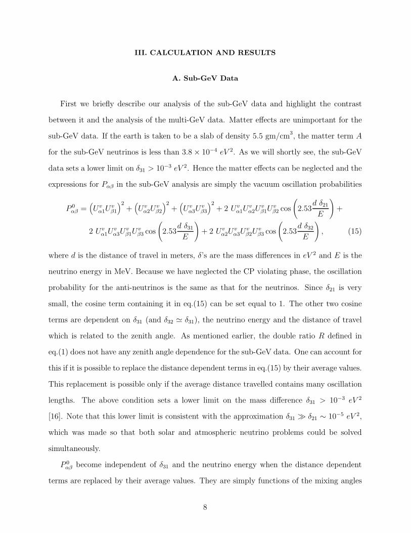
III. CALCULATION AND RESULTS

A. Sub-GeV Data

First we briefly describe our analysis of the sub-GeV data and highlight the contrast

between it and the analysis of the multi-GeV data. Matter effects are unimportant for the

sub-GeV data. If the earth is taken to be a slab of density 5.5 gm/cm3, the matter term A

for the sub-GeV neutrinos is less than 3.8 × 10−4 eV 2. As we will shortly see, the sub-GeV

data sets a lower limit on δ31 > 10−3 eV 2. Hence the matter effects can be neglected and the

expressions for Pαβ in the sub-GeV analysis are simply the vacuum oscillation probabilities

P 0

αβ =(

Uvα1U

vβ1

)2

+(

Uvα2U

vβ2

)2

+(

Uvα3U

vβ3

)2

+ 2 Uvα1U

vα2U

vβ1U

vβ2 cos

(

2.53d δ21E

)

+

2 Uvα1U

vα3U

vβ1U

vβ3 cos

(

2.53d δ31E

)

+ 2 Uvα2U

vα3U

vβ2U

vβ3 cos

(

2.53d δ32E

)

, (15)

where d is the distance of travel in meters, δ’s are the mass differences in eV 2 and E is the

neutrino energy in MeV. Because we have neglected the CP violating phase, the oscillation

probability for the anti-neutrinos is the same as that for the neutrinos. Since δ21 is very

small, the cosine term containing it in eq.(15) can be set equal to 1. The other two cosine

terms are dependent on δ31 (and δ32 ≃ δ31), the neutrino energy and the distance of travel

which is related to the zenith angle. As mentioned earlier, the double ratio R defined in

eq.(1) does not have any zenith angle dependence for the sub-GeV data. One can account for

this if it is possible to replace the distance dependent terms in eq.(15) by their average values.

This replacement is possible only if the average distance travelled contains many oscillation

lengths. The above condition sets a lower limit on the mass difference δ31 > 10−3 eV 2

[16]. Note that this lower limit is consistent with the approximation δ31 ≫ δ21 ∼ 10−5 eV 2,

which was made so that both solar and atmospheric neutrino problems could be solved

simultaneously.

P 0αβ become independent of δ31 and the neutrino energy when the distance dependent

terms are replaced by their average values. They are simply functions of the mixing angles

8

φ and ψ alone. In this approximation, the expression for the double ratio R can be written

as [16]

R =P 0

µµ + 1

rMCP 0

eµ

P 0ee + rMCP 0

µe

, (16)

where rMC is the Monte Carlo expectation of the ratio of number µ-like events to the

number of e-like events. From the sub-GeV data of Kamiokande, we find rMC = 1.912 and

R = 0.60+0.07−0.06±0.05 [5,16]. We take the allowed values of φ from our analysis of solar neutrino

data which restricts φ to be in the range 0 ≤ φ ≤ 500 [16]. We find the allowed region in

the φ − ψ plane by requiring the theoretical value calculated from eq.(16) to be within 1σ

or 1.6σ uncertainty of the experimental value. In our previous analysis we restricted the

range of ψ to be 0 ≤ ψ ≤ 450. However, given the assumptions we made about vacuum

mass eigenvalues, the most general possibility is to allow ψ to vary between 0 and 900 [20].

The new region allowed by the sub-GeV data, where φ was restricted by the solar neutrino

data and ψ is allowed to vary between 0 to 900, is shown in Figure 1. The region between

the solid lines is the parameter space which satisfies the experimental constraints at 1σ level

whereas the region between dashed lines satisfies the experimental constraints at 1.6σ level.

One important point to be noted in this analysis is that the sub-GeV data place only lower

bound on δ31. The allowed region in φ− ψ plane is quite large.

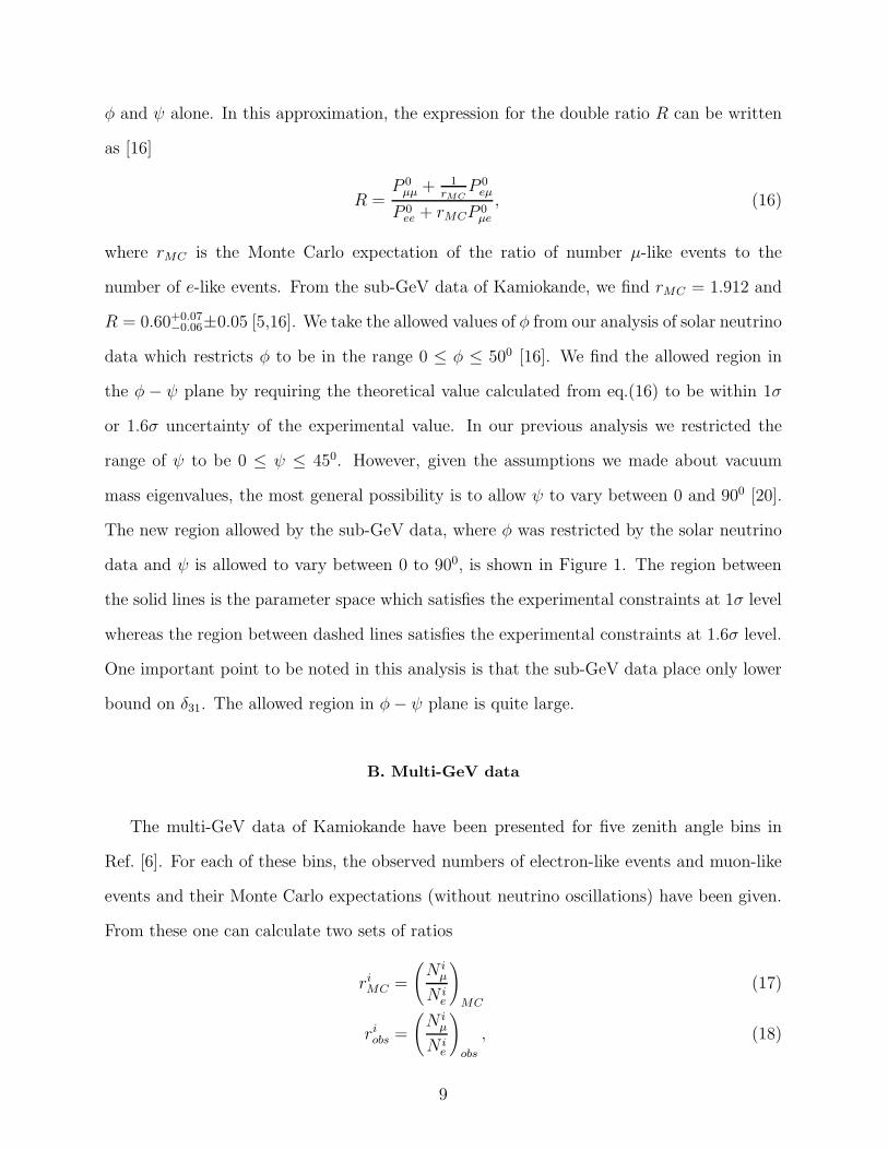
B. Multi-GeV data

The multi-GeV data of Kamiokande have been presented for five zenith angle bins in

Ref. [6]. For each of these bins, the observed numbers of electron-like events and muon-like

events and their Monte Carlo expectations (without neutrino oscillations) have been given.

From these one can calculate two sets of ratios

riMC =

(

N iµ

N ie

)

MC

(17)

riobs =

(

N iµ

N ie

)

obs

, (18)

9

and the set of double ratios

Riobs = ri

obs/riMC (19)

for each bin i = 1, 2, ..., 5. We summarize the multi-GeV data of Kamiokande [6] in Table I.

The µ-like events are subdivided into fully contained (FC) and partially contained (PC)

events whereas all the e-like events are fully contained. The efficiency of detection for each

type of event is different and is a funtion of the neutrino energy. Thus we have three detection

efficiencies εµFC(E), εµ

PC(E) and εe(E). We obtained these efficiencies from Kamiokande

Collaboration [21].

The expected number of µ-like and e-like events, in the absence of neutrino oscillations,

is given by

N iµ|M.C. =

∫

[

φiνµ

(E)σ(E) + φiνµ

(E)σ(E)]

(εµFC(E) + εµ

PC(E)) dE (20)

N ie|M.C. =

∫

[

φiνe

(E)σ(E) + φiνe

(E)σ(E)]

εe(E)dE (21)

where φ’s are the fluxes of the atmospheric neutrinos at the location of Kamiokande. These

are tabulated in Ref. [1] as functions of the neutrino energy (from E = 1.6 GeV to E = 100

GeV) and the zenith angle. σ and σ are the charged current cross sections of neutrinos and

anti-neutrinos respectively with nucleons. The cross section is the sum of the quasi-elastic

scattering and the deep inelastic scattering (DIS). The values for quasi-elastic scattering

are taken from Gaisser and O’Connel [22] and those for the DIS are taken from Gargamelle

data [23]. In calculating the DIS cross section, we took the lepton energy distribution to

be given by the scaling formula (which is different for neutrinos and anti-neutrinos) and

integrated dσ/dElep from the minimum lepton energy Emin = 1.33 GeV to the maximum

lepton energy Emax = Eν −mπ. The maximum lepton energy is chosen by defining DIS to

contain at least one pion in addition to the charged lepton and the baryon. The differences

in the fiducial volumes and exposure times for fully contained and partially contained events

have been incorporated into the detection efficiency εµPC(E). From equations (20) and (21)

we calculate our estimation of the Monte Carlo expectation of riMC , the ratio of the µ-like

10

events to the e-like events. The numbers we obtain are within 10% of the values quoted

by Kamiokande collaboration in Ref. [6]. The differences could be due to the different set

fluxes used [24] and due to the simple approximation we made for the cross sections.

In the presence of oscillations, the number of µ-like and e-like events are given by

N iµ|osc =

∫

[

φiνµPµµσ + φi

νµPµµσ + φi

νePeµσ + φi

νePeµσ

]

(εµFC + εµ

PC) dE (22)

N ie|osc =

∫

[

φiνePeeσ + φi

νePeeσ + φi

νµPµeσ + φi

νµPµeσ

]

εedE (23)

where Pαβs are the probabilities for neutrino of flavor α to oscillate into flavor β, derived

in the last section. These oscillation probabilities are functions of the distance of travel

d, the mixing angles φ and ψ, the mass difference δ31 and the matter term A. These are

calculated using the formulae in eqs. (8), (9), (10) and (14). The probability of oscillation for

anti-neutrinos Pαβ, in general, is different from Pαβ because of the different A dependence.

From equations (22) and (23) we can calculate the ratio of µ-like events to e-like events

in the presence of oscillations to be

riosc =

(

N iµ

N ie

)

osc

(24)

and the double ratio

Riosc =

riosc

riMC

. (25)

If the atmospheric neutrino deficit is due to neutrino oscillations, then the double ratios

Riosc given in eq. (25) should be within the range of the corresponding observed double ratios

Riobs, which are given in Table I. We searched for the values of the neutrino parameters φ, ψ

and δ31 for which the predicted values of Riosc satisfy the experimental constraints on the

double ratios for all the five bins. The ranges of variation in the three parameters are

1. 0 ≤ φ ≤ 500. This is the range of φ allowed by the solar neutrino problem. For

this range of φ, there exist values of δ21 and ω such that all the three solar neutrino

experiments can be explained [16,25].

11

2. 0 ≤ ψ ≤ 900. ψ is varied over its fully allowed range.

3. 10−3 eV 2 ≤ δ31 ≤ 10−1 eV 2. The lower limit is given by the sub-GeV data and the

upper limit is the largest value allowed by the two flavor analysis of the multi-GeV

data by Kamiokande [6].

The results are plotted in Figures 2, 3 and 4. Figure 2 gives the projection of the allowed

region on the φ− ψ plane, Figure 3 gives the projection on the φ− δ31 plane and Figure 4

gives the projection on the ψ − δ31 plane. The solid lines enclose the regions of parameter

space whose predictions lie within the experimental range given by 1σ uncertainties. The

broken lines enclose regions whose predictions fall within range given by 1.6σ uncertainties.

As seen from Table I, the uncertainties in bin 5, which has 〈cos θ〉 = 0.8, are quite large

compared to the uncertainties in the other four bins. Morevoer, r5obs is greater than r5

MC

through most of its range. Hence the double ratio R5obs > 1 for most of its range. The Monte

Carlo expectation of the electron neutrino flux is less than that of the muon neutrino flux

and the oscillation probabilities Pαβ are all less than 1. Using these facts, one can show from

eqs. (17) and (24) that, in general, riosc ≤ ri

MC or Riosc ≤ 1. Therefore, the region of overlap

between R5obs and R5

osc is very small. It is 0.9 − 1.0 for 1σ uncertainties. It is possible that

this small overlap is imposing a very strong constraint, leading to a situation where the bin

with the largest uncertainty is essentially controlling the allowed values of the parameters.

Because of this unsatisfactory situation, we redid the analysis ignoring the constraint from

bin 5. We searched for regions of parameter space for which the values of Riosc are within

the ranges of corresponding Riobs for only the first four bins.

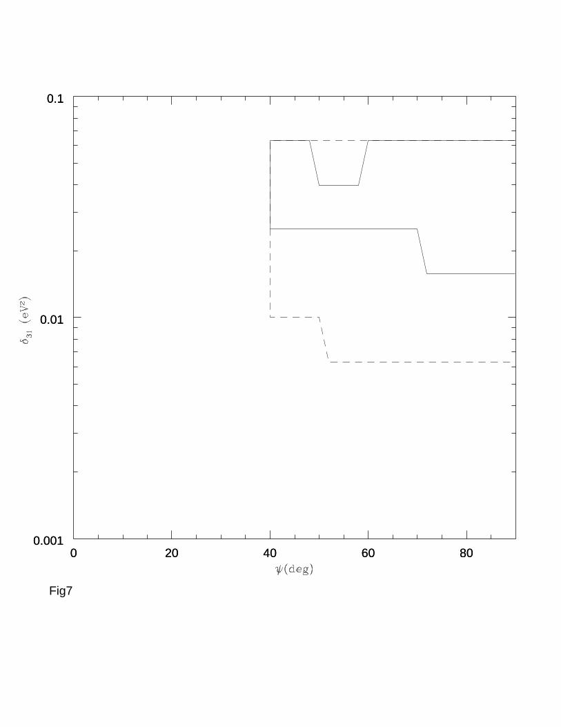
The results of the 4 bin analysis are plotted in Figures 5, 6 and 7. Figure 5 gives the

projection of the allowed region on the φ − ψ plane, Figure 6 gives the projection on the

φ−δ31 plane and Figure 7 gives the projection on the ψ−δ31 plane. As before, the solid lines

enclose the regions satisfying 1σ vetoes and the broken lines enclose regions allowed by 1.6σ

vetoes. Comparing the corresponding figures we find that the allowed values of parameters

for the 4 bin fit are the almost identical to those from the 5 bin fit at 1.6σ level. The allowed

12

regions at 1σ level are somewhat larger compared to the 5 bin fit. This is not surprising

because the bin 5 imposes a very strong constraint at 1σ level. If this constraint is relaxed,

then a somewhat larger region is allowed. The 4 bin fit shows that the 5th bin, which has

the largest uncertainty, does not exercise undue influence on the selection of the parameter

space.

IV. DISCUSSION AND CONCLUSIONS

The parameter space shown in Figures 1 to 4 , together with the allowed values for ω and

δ21 from our earlier work [16], provides a complete solution to the solar and the atmospheric

neutrino problems in the framework of three flavor neutrino oscillations. The salient features

of the results of the multi-GeV analysis are:

• Most of the parameter space allowed by the multi-GeV data is a subset of the space

allowed by the sub-GeV data.

• The range of δ31 allowed by 1σ vetoes is extremely narrow. It is very close to the best

fit value given by the two flavor analysis of Kamiokande.

• The value of ψ is always large (ψ ≥ 400) and ψ = 900 is allowed.

• In the region allowed by 1σ vetoes φ is always non-zero. φ = 0 is allowed only at 1.6σ

vetoes.

From the parametrization of Uv, effective two level mixings can be obtained for the

following choices of the angles:

• νe ↔ νµ for ψ = 900,

• νe ↔ ντ for ψ = 0 and

• νµ ↔ ντ for φ = 0.

13

Any solution to the atmospheric neutrino problem should suppress the muon neutrinos,

enhance the electron neutrinos or do both. The νe ↔ ντ channel, which suppresses electron

neutrinos but leaves muon neutrinos untouched, cannot account for the atmospheric neutrino

problem. Hence any solution of atmospheric neutrino problem should be away from the

effective two flavor νe ↔ ντ oscillations. The large value of the angle ψ is just a reflection

of this fact. The allowed region includes the value ψ = 900. Then the atmospheric neutrino

problem is explained purely in terms of the two flavor oscillations between νe ↔ νµ, with

the relevant mass difference being δ31. In this case, the solar neutrino problem is solved by

νe → ντ oscillation which is determined by the mass difference δ21 (and the mixing angles ω

and φ).

How important are the matter effects in the analysis of the multi-GeV data? It can be

seen from figures 2(d)-2(f) of Ref. [6] that most of the expected multi-GeV events are caused

by neutrinos with energies less than 10 GeV (over 80% for muon-like events and over 90% for

electron-like events). The matter term, for a neutrino of energy 5 GeV, is about 2×10−3eV 2.

Since the initial range we considered for δ31 varied from 10−3 eV 2 to 0.1 eV 2, apriori one

must include the matter effects in the expressions for the oscillation probabilities. However,

the value of δ31 in the allowed region, especially for the 1σ vetoes, where it is about 0.03 eV 2,

is much larger than the matter term. Therefore, it is likely that the matter effects may not

play an important role in determining the allowed parameter regions in the analysis of the

multi-GeV data. To check this we reran our program with the matter term set equal to zero.

With this change, the double ratios Riosc, defined in equation (24), changes by about 10% in

the first bin and by about 5% in the second bin. There is no discernible change in the other

three bins. Since the errors in Riobs are about 30%, these small changes in Ri

osc do not lead to

any apprecialble change in the allowed regions of the parameter space. However, the effect

of matter terms may become discerible when more accurate data from Super Kamiokande

become available.

Since the earth matter effects seem to play no role in the determination of the parameter

space, can one interpret the observed zenith angle dependence purely in terms of vacuum

14

oscillations? For an energy of 5 GeV, the mass square difference 10−2 eV 2 corresponds to

an oscillation length of about 1200 Km. Thus bins 1 and 2 contain many oscillation lengths

and the second and the third cosine terms in the vacuum oscillation probability, given in

equation (15), average out to zero. For bins 4 and 5 the cosine terms are almost 1. In bin 3,

these terms take some intermediate value. Therefore we have large suppression in the first

two bins, almost no suppression in the last two bins and moderate suppression in the middle

bin.

Eventhough matter terms play no important role in the multi-GeV analysis, νe ↔ νµ

oscillations provide a better fit to data compared to νµ ↔ ντ oscillations. In νµ ↔ ντ

oscillations, the νµ flux is suppressed whereas the νe flux is untouched. Thus the double

ratios Riosc do become less than 1 but the large suppression observed in bins 1 and 2 is

difficult to achieve via this channel. For νe ↔ νµ oscillations, the νµ flux is reduced and νe

flux is increased. This occurs even when Pµe = Peµ, which is the case for vacuum oscillations,

because the flux of νµ is roughly twice the flux of νe before oscillations. Hence the double

ratios Riosc are smaller for the case of νe ↔ νµ oscillations compared to the case of νµ ↔ ντ

oscillations and they fit the data better.

We now make a brief comment on the LSND results on the search for νµ → νe oscillations

[18] in the context of our analysis of atmospheric neutrinos. The LSND collaboration gives

an oscillation probability Pµe = (3.1+1.1−1.0 ± 0.5)× 10−3 for muon anti-neutrinos in the energy

range 20 − 60 MeV. In the framework described in section II, the oscillation probability

relevant for the LSND experiment is the vacuum oscillation probability

P 0

µe = P 0

µe = sin2 2φ sin2 ψ sin2

(

1.27d δ31E

)

. (26)

Note that both φ and ψ have to be non-zero for Pµe to be non-zero. In the region allowed

by the 1σ vetoes of the multi-GeV atmospheric neutrino data we have

Minimum(

sin2 2φ sin2 ψ)

≃ 0.04 for φ ≃ 80, ψ ≃ 400

Maximum(

sin2 2φ sin2 ψ)

≃ 1 for φ ≃ 400, ψ ≃ 900.

15

Substituting these values and the oscillation probability obtained by LSND in eq. (26), we

obtain

0.001 ≤ sin2

(

1.27d δ31E

)

≤ 0.1. (27)

For the LSND experiment the distance d = 30 meters. Taking the average energy to be

〈E〉 = 40 MeV, we obtain the range of δ31 to be

0.03 eV 2 ≤ δ31 ≤ 0.3 eV 2. (28)

From the analysis of multi-GeV atmospheric neutrino data we have the upper limit on

δ31 ≤ 0.06 eV 2 (Figures 3 and 4). Hence there is a small region of overlap between the range

of neutrino parameters required by the atmospheric neutrino data and the LSND data. This

suggests that the standard three flavor analysis can accommodate all the data so far [26]

and perhaps a fourth sterile neutrino is not needed.

In conclusion, we have analyzed the atmospheric neutrino data of Kamiokande in the

context of three flavor neutrino oscillations. We took into account both the zenith angle

dependence of the multi-GeV data and the matter effects due to the propagation of the

neutrinos through the earth. We obtained the regions in neutrino parameters which solve

both the solar and the atmospheric neutrino problems. We found that the matter effects

have negligible influence on atmopsheric neutrinos even in the multi-GeV range. The allowed

regions of the parameter space with or without matter effects are almost identical.

As we finished this work, we came across a preprint by Fogli et al [27]. They have

analyzed the sub-GeV data from various experiments and the zenith angle dependent multi-

GeV data from Kamiokande. Although a detailed comparison is difficult, qualitatively our

results agree with theirs.

Acknowledgements: We are grateful to M. V. N. Murthy for collaboration during the

earlier part of this work and for a critical reading of the manuscript. We are specially

grateful to Prof. Kajita of the Kamiokande Collaboration for supplying us with the detection

16

efficiencies of the Kamiokande detector. We thank S. R. Dugad, Rahul Sinha, N. K. Mondal

and K. V. L. Sarma for numerous discussions during the course of this work. We also thank

Jim Pantaleone, Sandip Pakvasa and the referee for critical comments.

17

REFERENCES

[1] M. Honda et al, Phys. Rev. D52, 4985 (1995).

[2] V. Agrawal et al, Phys. Rev. D53, 1314 (1996).

[3] IMB Collaboration: D. Casper et al., Phys. Rev. Lett. 66, 2561(1991); R. Becker-Szendy

et al., Phys. Rev. D46, 3720(1992).

[4] IMB Collaboration observed a deficit of muon-like events in their data compared to the

Monte-Carlo prediction as early as 1986 and have speculated whether this deficit is due

to non-Standard Physcis. T. J. Haines et al, Phys. Rev. Lett. 57, 1986 (1986).

[5] Kamiokande Collaboration: K. S. Hirata et al, Phys. Lett. B280, 146 (1992).

[6] Kamiokande Collaboration: Y. Fukuda et al, Phys. Lett. B335, 237 (1994).

[7] V. Barger et al, Phys. Rev. D22, 2718 (1980).

[8] G. V. Dass and K. V. L. Sarma, Phys. Rev. D30, 80 (1984).

[9] J. Pantaleone, Phys. Rev. D49, R2152 (1994).

[10] S. Goswami, K. Kar and A. Raychaudhury, CUPP-95/3 May 1995, hep-ph/9505395;

S. Goswami, CUPP-95/4 July 1995, hep-ph/9507212.

[11] S. M. Bilenky, C. Giunti and C. W. Kim, hep-ph 9505301.

[12] C. Giunti, C. W. Kim and J. D. Kim, Phys. Lett. 352B, 357 (1995).

[13] D. Harley, T. K. Kuo and J. Pantaleone, Phys. Rev. D47, 4059 (1993).

[14] G. Fogli, E. Lisi and D. Montanino, Phys. Rev. D49, 3626 (1994); Astropart. Phys. 4,

177 (1995).

[15] A. S. Joshipura and P. I. Krastev, Phys. Rev. D 50, 3484 (1994).

[16] M. Narayan et al, Phys. Rev. D53, 2809 (1996).

18

[17] O. Yasuda, TMUP-HEL-9603 February 1996, hep-ph/9602342

[18] LSND Collaboration: C. Athanassopoulos et al, Los Alamos Preprint LA-UR-96-1582,

nucl-ex/9605003.

[19] L. Wolfenstein, Phys. Rev. D17, 2369 (1978); D20, 2634 (1979).

[20] We thank J. Pantaleone for pointing this out to us.

[21] We thank Prof. T. Kajita of the Kamiokande Collaboration for providing us with the

efficiencies for the detection of various types of events.

[22] T. K. Gaisser and J. S. O’Connell, Phys. Rev D34, 822 (1986).

[23] P. Musset and J. P. Vialle, Phys. Rep. 39C, 1 (1978).

[24] Kamiokande Collaboration, in their analysis in Ref. [6], used the fluxes from G. Barr,

T. K. Gaisser and T. Stanev, Phys. Rev. D39, 3532 (1989) for eν < 3 GeV and those

from L. V. Volkova, Sov. J. Nucl. Phys. 31, 784 (1980) for Eν > 10 GeV . For energies

between 3 and 10 GeV they have smoothly interpolated between the two fluxes.

[25] G. L. Fogli, E. Lisi and D. Montanino, Phys. Rev. D54, 2048 (1996).

[26] C. Y. Cardall and G. M. Fuller, Phys. Rev. D53, 4421 (1996).

[27] G. L. Fogli, E. Lisi, D. Montanino and G. Scioscia, Preprint Number IASSNS-AST-

96/41, hep-ph/9607251.

19

TABLES

Bin No. 〈cosθ〉 〈distance〉 in Km riMC ri

obs Riobs

1 -0.8 10,210 3.0 0.87+0.36−0.21 0.29+0.12

−0.07

2 -0.4 5,137 2.3 1.06+0.39−0.30 0.46+0.17

−0.13

3 0.0 832 2.1 1.07+0.32−0.23 0.51+0.15

−0.11

4 0.4 34 2.3 1.45+0.51−0.34 0.63+0.22

−0.16

5 0.8 6 3.0 3.9+1.8−1.2 1.3+0.6

−0.4

TABLE I. Zenith angle dependent data from Kamiokande [6]

20

FIGURES

FIG. 1. Allowed region in φ − ψ plane by the sub-GeV data (with δ31 ≥ 10−3 eV 2) at 1σ

(enclosed by solid lines) and at 1.6σ (enclosed by broken lines)

FIG. 2. Allowed region in φ − ψ plane by 5 bin analysis of multi-GeV data

(with 10−3 eV 2 ≤ δ31 ≤ 10−1 eV 2) at 1σ (enclosed by solid lines) and at 1.6σ (enclosed by

broken lines)

FIG. 3. Allowed region in φ−δ31 plane by 5 bin analysis of multi-GeV data (with 0 ≤ ψ ≤ 900)

at 1σ (enclosed by solid lines) and at 1.6σ (enclosed by broken lines)

FIG. 4. Allowed region in ψ−δ31 plane by 5 bin analysis of multi-GeV data (with 0 ≤ φ ≤ 500)

at 1σ (enclosed by solid lines) and at 1.6σ (enclosed by broken lines)

FIG. 5. Allowed region in φ − ψ plane by 4 bin analysis of multi-GeV data

(with 10−3 eV 2 ≤ δ31 ≤ 10 eV 2) at 1σ (enclosed by solid lines) and at 1.6σ (enclosed by bro-

ken lines)

FIG. 6. Allowed region in φ−δ31 plane by 4 bin analysis of multi-GeV data (with 0 ≤ ψ ≤ 900)

at 1σ (enclosed by solid lines) and at 1.6σ (enclosed by broken lines)

FIG. 7. Allowed region in ψ−δ31 plane by 4 bin analysis of multi-GeV data (with 0 ≤ φ ≤ 500)

at 1σ (enclosed by solid lines) and at 1.6σ (enclosed by broken lines)

21

0 10 20 30 40 500

20

40

60

80

0 10 20 30 40 500

20

40

60

80

Fig1

0 10 20 30 40 500

20

40

60

80

0 10 20 30 40 500

20

40

60

80

Fig2

0 10 20 30 40 500.001

0.01

0.1

0 10 20 30 40 500.001

0.01

0.1

Fig3

0 20 40 60 800.001

0.01

0.1

0 20 40 60 800.001

0.01

0.1

Fig4

0 10 20 30 40 500

20

40

60

80

0 10 20 30 40 500

20

40

60

80

Fig5

0 10 20 30 40 500.001

0.01

0.1

0 10 20 30 40 500.001

0.01

0.1

Fig6

0 20 40 60 800.001

0.01

0.1

0 20 40 60 800.001

0.01

0.1

Fig7